CoVaR�

Tobias Adriany

Federal Reserve Bank of New YorkMarkus K. Brunnermeierz

Princeton University

This Version: March 12, 2009- incomplete revision -

AbstractWe propose a measure for systemic risk: CoVaR, the Value at Risk (VaR)

conditional on an institution (or the whole �nancial sector) being under dis-tress. We argue for regulatory requirements that are based on the di¤erencebetween CoVaR and VaR, capturing an institution�s (marginal) contribution tosystemic risk. Countercyclical regulation should take institution�s characteristicslike maturity mismatch and leverage into account to the extent that they predictsystemic risk contributions.

Keywords: Value at Risk, Systemic Risk, Adverse Feedback Loop, EndogenousRisk, Risk Spillovers, Financial ArchitectureJEL classi�cation: G10, G12

�Please apologize typos of this intermediate version.Special thanks goes to Hoai-Luu Nguyen for excellent research assistantship. The authors would alsolike to thank René Carmona, Stephen Brown, Xavier Gabaix, Beverly Hirtle, Jon Danielson, JohnKambhu, Arvind Krishnamurthy, Burton Malkiel, Maureen O�Hara, Matt Pritsker, José Scheinkman,Kevin Stiroh and seminar participants at the NBER, Columbia University, Princeton University,Cornell University, Rutgers University, the Bank for International Settlement, Mannheim University,Hong Kong University of Science and Technology, University of Arizona, Arizona State University,University of North Carolina, Duke University, and the Federal Reserve Bank of New York for helpfulcomments. We are grateful for support from the Institute for Quantitative Investment ResearchEurope (INQUIRE award). Brunnermeier also acknowledges �nancial support from the Alfred P.Sloan Foundation. Previous versions of the paper were circulated under the titles �Hedge Fund TailRisk.�Early versions of the paper were presented at the New York Fed and Princeton University inFebruary and March 2007. The views expressed in this paper are those of the authors and do notnecessarily represent those of the Federal Reserve Bank of New York or the Federal Reserve System.

yFederal Reserve Bank of New York, Capital Markets, 33 Liberty Street, New York, NY 10045,http://nyfedeconomists.org/adrian, email: tobias.adrian@ny.frb.org.

zPrinceton University, Department of Economics, Bendheim Center for Finance, Prince-ton, NJ 08540-5296, NBER, CEPR, CESIfo, http://www.princeton.edu/~markus, e-mail:markus@princeton.edu.

1 Introduction

During times of �nancial crisis, losses tend to spread across �nancial institutions,

threatening the �nancial system as a whole.1 Measures of systemic risk that capture

risk spillovers and tail risk correlations should form the basis of any macro-prudential

regulation.

The most common measure of risk used by �nancial institutions� the Value at Risk

(VaR)� focuses on the risk of an individual institution in isolation. The �%-VaR is the

maximum dollar loss within the (1� �%)-con�dence interval; see, e.g., Jorion (2006).

However, a single institution�s risk measure does not necessarily re�ect systemic risk �

the risk that the stability of the �nancial system as a whole is threatened. A measure for

systemic risk should achieve two objectives. First, it should indicate which institutions

are likely to be in �nancial di¢ culties should a systemic risk event occur. Second,

it should jointly measure (i) how �nancial di¢ culties of one institution spill over to

others and (ii) how �nancial tail risk is correlated among the main �nancial institutions.

Following the classi�cation in Brunnermeier, Crocket, Goodhart, Perssaud, and Shin

(2009), the �rst group of institutions are �individually systemic�because they are so

massively interconnected and large that they can cause negative risk spillover e¤ects on

others. The second group of institutions are �systemic as part of a herd�because they

are exposed to a common risk factor. Since it is not essential to distinguish whether

an institution is individually systemic or as part of a herd, the risk measure does not

need to identify a causal relationship.

In this paper, we propose such a measure for systemic risk that covers both ob-

1Examples include the 1987 equity market crash which started by portfolio hedging of pensionfunds and led to substantial losses of investment banks; the 1998 crisis started with losses of hedgefunds and spilled over to the trading �oors of commercial and investment banks; and the 2007/08crisis spread from SIVs to commercial banks and on to hedge funds and investment banks, see Brady(1988), Rubin, Greenspan, Levitt, and Born (1999), and Brunnermeier (2009).

1

jectives. We call our risk measure CoVaR, where the �Co�stands for conditional,

comovement, contagion, or contributing. In general terms, it is de�ned as the VaR

conditional on either the whole �nancial sector or the particular institution being in

distress. For determining which institutions are likely to experience distress in case

of a systemic event, we condition the VaR of each institution on the event that the

index return of the �nancial sector is at its VaR level. Note that the likelihood of

being in distress in case of a systemic event depends to a large extent on the insti-

tution�s funding strategy (leverage, maturity mismatch etc.) in addition to its asset

holdings. To address the question to what extent a particular institution contributes

(in a non-causal sense) to the overall systemic risk (by being in distress when there

is a system-wide distress), we reverse the conditioning. In this case, an institution�s

CoVaR is de�ned as the VaR of the whole �nancial sector conditional on this institu-

tion being in distress. The di¤erence between the CoVaR and unconditional �nancial

industry VaR, �CoVaR, captures the marginal contribution of a particular institution

(in a non-causal sense) to the overall systemic risk.

In practice, we argue for a change of the regulatory framework that emphasizes the

institution�s contribution to systemic risk and focuses not only on its individual risk.

More speci�cally, the degree an institution increases the CoVaR of the �nancial sector

or of a speci�c set of �nancial institutions (such as the institutions with access to the

discount window) should determine the macro-prudential regulation of that institution.

Capital and liquidity requirements should re�ect the potential for risk spillovers and

tail correlations. The aim is to internalize externalities and provide the incentive to

minimize systemic risk exposure.

Current risk regulation focuses on the risk of an individual institution (in isolation).

This leads, in the aggregate, to excessive risk along the systemic risk factors. To see

2

this more explicitly, consider two institutions, A and B, which report the same VaR,

but while institution A�s CoVaR=VaR, institution B�s CoVaR largely exceeds its VaR.

Based on theirVaRs, both institutions seem to appear to be equally risky. However, the

high CoVaR of institution B indicates that it is more correlated/exposed to system

risk. Since system risk carries a higher risk premium, institution B will outshine

institution A and competitive pressure will force institution A to follow suit. Imposing

stricter regulatory requirements on institution B would break this herding tendency.

One might argue that regulating institutions�VaR might be su¢ cient as long as each

institution�s CoVaR goes hand in hand with its VaR. This is not the case, since (i) it is

not desirable that institution A increases its contribution to systemic risk by following

a strategy similar to institution B and (ii) there is no one-to-one connection between

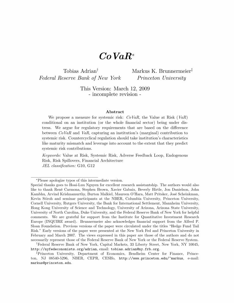
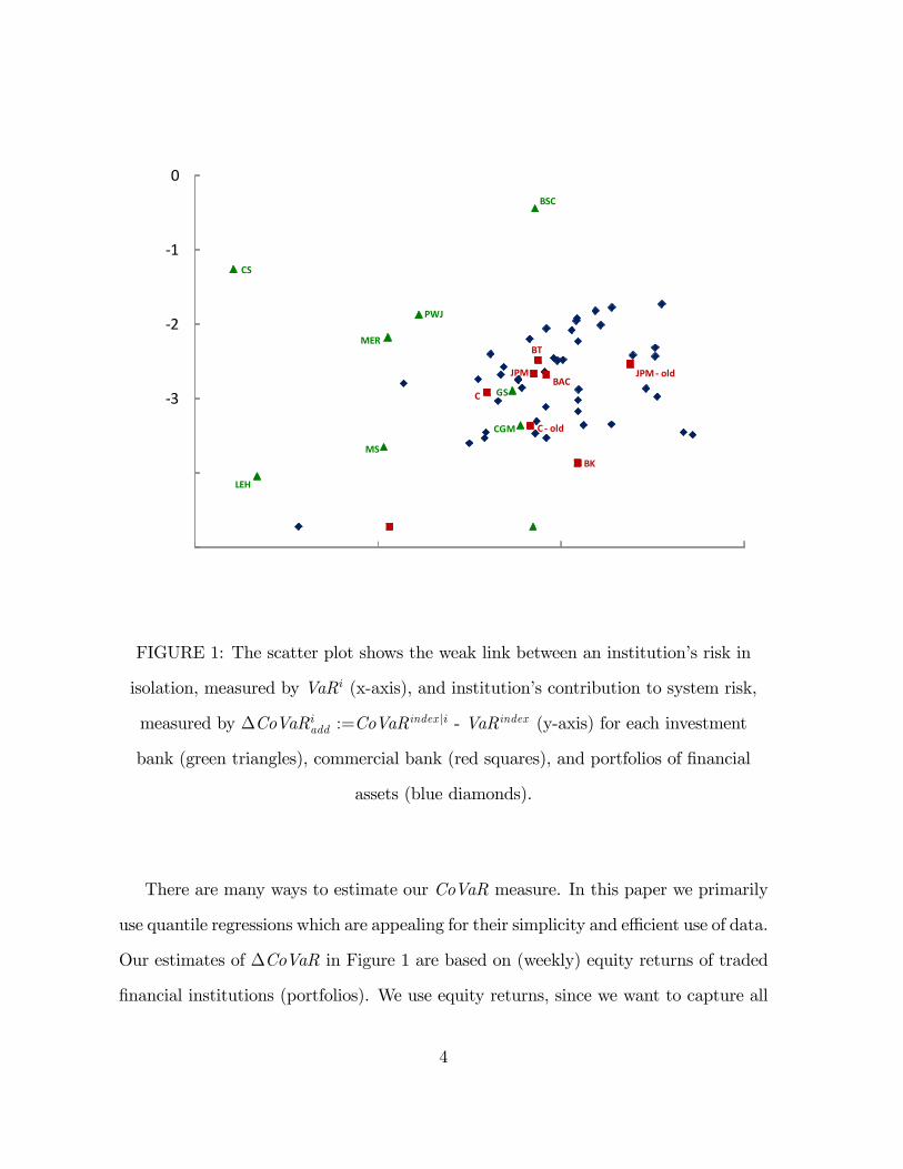
institutions CoVaR (y-axis) and VaR (x-axis) as Figure 1 shows. Overall, Figure 1

questions the sole focus on VaR as the current bank regulation based on Basel II does.

3

­5

­4

­3

­2

­1

0

­21 ­16 ­11 ­6

∆CoVaR

i add

VaRi

Portfolios Commercial Banks Investment Banks

BSC

MER

LEH

MS

C

JPMBAC

GS

JPM ­ old

C ­ old

CS

PWJ

BK

BT

CGM

FIGURE 1: The scatter plot shows the weak link between an institution�s risk in

isolation, measured by VaRi (x-axis), and institution�s contribution to system risk,

measured by �CoVaRiadd :=CoVaRindex ji - VaRindex (y-axis) for each investment

bank (green triangles), commercial bank (red squares), and portfolios of �nancial

assets (blue diamonds).

There are many ways to estimate our CoVaR measure. In this paper we primarily

use quantile regressions which are appealing for their simplicity and e¢ cient use of data.

Our estimates of �CoVaR in Figure 1 are based on (weekly) equity returns of traded

�nancial institutions (portfolios). We use equity returns, since we want to capture all

4

forms of risk, including not only the risk of adverse asset price movements, but� equally

importantly� also funding liquidity risk. In other words, focusing exclusively on the

quality of an institution�s asset portfolio is insu¢ cient, since it is the funding structure,

especially the asset-liability maturity mismatch, that exposes an institution to systemic

risk. Ideally, one would like to base the risk measure on exact asset composition and

funding structure especially as they can change rapidly over time. For hedge funds�

CoVaR measures we rely on reported returns.

One reason why institutions�CoVaR estimates might not line up well with the VaR

estimates is that their portfolio strategy might have changed over time. For example,

a particular institution might have been very levered in the 1990s but may have only

a low leverage ratio in the 2000s. Its overall estimated CoVaR re�ects a mixture of

both leverage ratios. We attempt to control for this e¤ect by repeating the analysis for

portfolios that are sorted based on leverage, maturity mismatch, volatility, etc.

The second part of the paper addresses the problem that any (empirical) risk mea-

sure su¤ers from the fact that �tail observations� are� by de�nition� rare. After a

string of good news, risk seems tamed, but, when a new tail event occurs, the esti-

mated risk measure may sharply increase. This problem is most pronounced if the data

samples are short. Hence, regulatory requirements that are naively based on estimated

risk measures would be stringent during a crisis and lax during a boom. This intro-

duces procyclicality �exactly the opposite of the goal of e¤ective regulation. In order

to derive a countercyclical risk measure, we derive the �CoVaR for each institution

using the full set of data. We �rst estimate it conditional on macro variables like slope

of yield curve, aggregate credit spread, and implied market volatility from VIX. Using

panel regressions we then relate these time-varying �CoVaR measures to institutions�

maturity mismatch, leverage, and book-to-market. We do so contemporaneously and

5

in a predictive sense. The regression coe¢ cients indicate how one should weigh the

di¤erent funding liquidity measures in determining the capital charge or Pigouvian tax

imposed on various �nancial institutions. The predictive regressions allow the regu-

lator to act in advance. Of course, any empirical analysis is limited and has to be

complemented with �theorizing�, especially when the banking model changes.

Related Literature. Our co-risk measures can be interpreted in light of recent eco-

nomic theories of �nancial sector ampli�cation. While we do not test any particular

theory, CoVaR is meaningful in economic settings where �nancing constraints of �-

nancial institutions are linked to risk. As measured risk increases, margin and capital

requirements widen, forcing institutions to unwind. This tends to increase market risk,

thus leading to further increases of measured risk.

Brunnermeier and Pedersen (2009) propose a theory of margin spirals, where bal-

ance sheet constraints lead to risk spillovers among �nancial institutions. Adrian and

Shin (2009) derive a micro foundation for the use of VaR by �nancial institutions

and analyze risk spillovers for �nancial systems of interlocked balance sheets. Kyle

and Xiong (2001) provide a model of contagion among �nancial institutions where the

interaction of risk spillovers and wealth e¤ects leads to institutional contagion.

Our paper can also be linked to several other strands of literatures. First, our paper

contributes to the growing literature that sheds light on the link between hedge funds

and the risk of a systemic crisis. Boyson, Stahel, and Stulz (2006) document contagion

across hedge fund styles using logit regressions. Chan, Getmansky, Haas, and Lo (2006)

document an increase in correlation across hedge funds, especially prior to the LTCM

crisis and after 2003. Adrian (2007) points out that the increase in correlation since

2003 is due to a reduction in volatility �a phenomenon that occurred across many

6

�nancial assets �rather than an increase in covariance.

Second, our work relates to the large literature in international �nance that focuses

on cross-country spillovers. For example, King and Wadhwani (1990) document an

increase in correlation across stock markets during the 1987 crash, which in itself �

as Forbes and Rigobon (2002) argue � is only evidence for interdependence but not

contagion, since estimates of correlation tend to go up when volatility is high. Claessens

and Forbes (2001) and the articles therein provide an overview. In contrast to these

papers, our analysis focuses on volatility spillovers. The most common method to test

for volatility spillover is to estimate GARCH processes, as e.g. Hamao, Masulis, and

Ng (1990) do for international stock market returns. While GARCH processes allow

for time-variation in conditional volatility, they assume that extreme returns follow the

same return distribution as the rest of returns. Hartman, Straetmans, and de Vries

(2004) avoid this criticism by developing a contagion measure that focuses on extreme

events. Building on extreme value theory, they estimate the expected number of market

crashes given that at least one market crashes. However, extreme value theory works

best for very low quantiles (see Danielsson and de Vries (2000)). This motivates Engle

and Manganelli (2004) to develop CAViaR that � like our approach �makes use of

quantile regressions as initially proposed by Koenker and Bassett (1978) and Bassett

and Koenker (1978). While Engle and Manganelli�s CAViaR focuses on the evolution

of quantiles over time, we study risk spillover e¤ects across �nancial institutions as

measured by our CoVaR. More recently, Rossi and Harvey (2007) estimate time-varying

quantiles and expectiles using a state space signal extraction algorithm. The machinery

developed by Engle and Manganelli (2004) and Rossi and Harvey (2007) could be used

to study the time variation of CoVaR.

The remainder of the paper is organized in four sections. In Section 2, we outline

7

the methodology. We de�ne CoVaRs, introduce time-variation and show how one could

implement a countercyclical �nancial regulation. In Section 3, we present estimates of

CoVaRs for commercial banks, investment banks, and hedge funds and relate them

to macro risk factors. In Section 4, we show to what degree CoVaRs depend on the

�nancial institutions�characteristics such as leverage, maturity mismatch, and size and

whether these variables help to predict future CoVaRs. We conclude in Section 5.

2 CoVaR Methodology

In this section, we �rst introduce our systemic co-risk measure, CoVaR, and then specify

two particular forms that are the focus of this paper. Subsequently, we introduce time-

varying CoVaRs by linking our CoVaR estimates to certain macro variables and �nally,

we outline how one can achieve a countercyclical �nancial regulation.

2.1 De�nition of CoVaR

Recall that VaRiq is implicitly de�ned as the q quantile, i.e.

Pr�Ri � VaRiq

�= q,

where Ri is the return of institution (or portfolio) i. Note that VaRiq is typically a

negative number. Practitioners usually switch the sign, a sign convention we will not

follow. It is also noteworthy that all our empirical results are expressed in percentage

returns. These can be transformed into dollar amounts by multiplying by total assets.

De�nition 1 We denote the CoVaRijjq , the VaRiq of institution (index) i conditional

on the (unconditional) VaR of institution (index) j. That is, CoVaRijq is implicitly

8

de�ned by q-quantile of the conditional probability distribution

Pr�Ri � CoVaRijjq jRj = VaRjq

�= q.

Institutions j�s contribution to CoVaRijjq is simply denoted by

�CoVaRijjq = CoVaRijjq �VaRiq,

The CoVaR is typically more negative than the unconditional VaR since condition-

ing on a �bad event�typically shifts the mean downwards and can even increases the

variance in an environment with heteroskedasticity. The CoVaR, unlike the covariance,

re�ects both shifts. In addition, CoVaR focuses on the tail distribution and, impor-

tantly, it is directional. That is, typically CoVaRijjq 6= CoVaRjjiq , since reversing the

conditioning matters. Note also, that we condition on the return Rj = VaRjq. This

ensures that the conditioning event is equally likely independently of whether one con-

ditions on the return of a risky or a less risky institution. (In contrast, conditioning

on an absolute return level would make the conditioning more extreme for less risky

institutions/indexes Rj.) Another attractive feature of CoVaR is that it can be easily

adopted for other �corisk-measures�. One of them is the co-expected-shortfall, Co-ES.

Expected shortfall has a number of advantages relative to VaR and can be calculated

as a sum of VaRs. In the same manner, Co-ES can be calculated as an integral of

CoVaRs.

Finally, the CoVaR de�nition can be applied to analyze the tail dependency across

two �nancial institutions or with respect to indexes. For example, one can calculate

the conditional Value at Risk of a particular investment bank conditional on the fact

9

that hedge funds are in �nancial di¢ culty. In this paper we put special emphasis on

the following two forms of CoVaR measures.

2.1.1 Exposure Measure: CoVaRiexp

To investigate which �nancial institutions are most exposed in the case of a systemic

�nancial crisis, we condition each individual institution�s VaRi on the event that the

portfolio of all �nancial institutions is in distress, i.e. is at its VaRindex level.

Pr�Ri � CoVaRijindexq jRindex = VaRindexq

�= q.

To simplify notation we call it CoVaRiexp , where the superscript stands for �systemic

risk exposure�of institution i.

2.1.2 Contribution Measure: CoVaRiadd

To investigate which �nancial institution i�s marginal contribution to systemic risk is

highest, we reverse the conditioning. That is, we calculate the Value of Risk of the

whole �nancial system conditional on institution i being in distress:

Pr�Rindex � CoVaRindex jiq jRi = VaRiq

�= q.

We denote it as CoVaRiadd , since the di¤erence to the unconditional VaR of the

�nancial system, �CoVaRiadd , measures how much this institution �adds� to overall

systemic risk (in returns). This measure captures externalities that arise because an

institution is �too big to fail�, or �too interconnected to fail�, or takes on positions

or relies on funding that can lead to crowded traded. Of course, ideally, one would

like to have a co-risk measure that satis�es a set of axioms as e.g. the Shapley value

10

does. Recall that the Shapley value measures the marginal contribution of a player to

a grand coalition.

Importantly, the CoVaRiadd measure does not distinguish whether the contribution

is causal or simply driven by a common factor. We view this as a virtue rather than

a disadvantage. To see this, suppose a large number of small hedge funds hold similar

positions and are funded in a similar way. That is, they are exposed to the same factors.

Now, if only one of the small hedge funds falls into distress, this will not necessarily

cause any systemic crisis. However, if this is due to a common factor all of hedge

funds, i.e. all which are �systemic as port of a herd�will be in distress. Hence, each

individual�s hedge fund co-risk measure should capture this, even though there is no

direct causal link and the CoVaRiadd measure does so.

2.1.3 Endogeneity of Systemic Risk

Note that each institution�s CoVaR is endogenous and depends on the other institu-

tions� risk taking. Hence, imposing a regulatory framework that internalizes exter-

nalities alters the CoVaR measures. We view the fact that CoVaR is an equilibrium

measure as a strength, since it adapts to changing environments and provides an incen-

tive for each institution to reduce its exposure to certain risk factors if other institutions

load excessively on it.

2.1.4 Equity Returns

Our analysis focuses on VaR-returns rather on absolute dollar amounts since it makes

a comparison across institutions of di¤erent sizes easier. More importantly, no capital

ratios have to be calculated since regulation can impose direct caps on the equity return

11

CoVaRiadd .2

We focus on equity returns since a �nancial institution�s risk is not only driven

by the riskiness of its assets but also by the risk of its funding structure. Ideally, one

would like to calculate the asset and funding risk across several trading desks separately

and relate them to each other. Without detailed P&L data for subdivisions of �rms,

however, it is best to rely on equity returns. Focusing on asset returns alone and

ignoring funding considerations �as the current bank regulatory framework does �is

in our view inferior to equity returns.

2.2 Time-variation in CoVaRt and VaRt

Applying our de�nition directly, we can only estimate a single CoVaR for each insti-

tution that is constant over time. To overcome this limitation, we pursue two modi-

�cations. First, to re�ect the fact that �nancial institutions��nancing strategy might

change over time, we also calculate the CoVaRs for portfolio sorts. Second, to capture

time variation that covaries with certain macro-variables and risk factors, we allow

time-variation along these factors.

2.2.1 Portfolio Sorts

While we are interested in estimating the evolution of the risk measures VaR and

CoVaR for individual �nancial institutions, the nature of any particular institution

might have changed drastically over the 1986-2008 sample period. In addition, many

of the individual banks merged with other organizations, and some went out of business.

One way to control for the changing nature of each individual institution is to form

2Current bank regulation requires that a bank�s Value-at-Risk in dollar amounts divided by itscapital does not exceed a certain threshold.

12

portfolios on particularly important balance sheet characteristics. In particular, we

form the following sets of quintile portfolios: maturity mismatch, leverage, cash to

assets, book to market, and equity volatility. Maturity mismatch is measured as short-

term debt - (cash + short-term investments) normalized by dividing it by total assets.

Leverage is the ratio of total assets to book equity. Equity volatility is estimated each

quarter from the daily equity return data. We form portfolios every quarter.

2.2.2 Time-variation linked to Macro Variables

To allow for time-variation we relate the CoVaR and the VaR to certain macro vari-

ables with whom they co-vary. We indicate time-varying (Co)VaRt with an additional

subscript t. Taking time-variation into account leads to a panel data set of (Co)VaRts

and reduces the problem that tail correlation are overestimated when volatility is high

(see e.g. Claessens and Forbes (2001)).

More speci�cally, we focus on the following �macro�factors to estimate the variation

of VaRs and CoVaRs across institutions and over time. The factors capture certain

aspects of risks. They are also liquid and easily tradable. We restrict ourselves to a

small set of risk factors to avoid over�tting the data. Our factors are:

(i) VIX which captures the implied future volatility in the stock market. This

implied volatility index is available on Chicago Board Options Exchange�s website.

(ii) a short term �liquidity spread�, de�ned as the di¤erence between the 3-month

repo rate and the 3-month bill rate measures the short-term counterparty liquidity risk.

We use the 3-month general collateral repo rate that is available on Bloomberg, and

obtain the 3-month Treasury rate, from the Federal Reserve Bank of New York.

(iii) The level of the 3-month term Treasury bill rate.

In addition we consider the following two �xed-income factors that are known to

13

be indicators in forecasting the business cycle and also predict excess stock returns

(Estrella and Hardouvelis (1991), Campbell (1987), and Fama and French (1989)):

(iv) the return to the slope of the yield curve, measured by the yield-spread between

the 10-year Treasury rate and the 3-months bill rate.

(v) the return to the credit spread between BAA rated bonds and the Treasury rate

(with same maturity of 10 years).

The last two factors are from the Federal Reserve Board�s H.15 release.3

2.3 Countercyclical Regulation based on Predictive Charac-

teristics

Instead of relating �nancial regulation directly to our�CoVaRit measure, we propose to

link them to more frequently observed variables that predict the�CoVaRit of a �nancial

institution in advance. This ensures that �nancial regulation is implemented in a pro-

active and countercyclical way. Like any tail risk measure, CoVaRt estimates rely on

3The literature has studied related factors for explaining hedge fund returns. Boyson, Stahel, andStulz (2006) use the S&P500, Russell 3000, change in VIX, FRB dollar index, Lehman US bond indexand the 3-Month Bill return as factors, but �unlike our study �they do not �nd a link between thesefactors and contagion. Agarwal and Naik (2004) also focus on tail risk. In addition to out of the moneyput and call market factors they use the Russell 3000, MSCI excluding US (bonds), MSCI emergingmarkets, HML, SMB, MOM, Salomon Government and corporate bonds, Salomon world governmentbonds, Lehman high yield, Federal Reserve trade weighted dollar index, GS commodity index andchange in default spread. Factors used in Fung and Hsieh (1997, 2001, 2002, 2003) di¤er dependingon the hedge fund style they analyze. An innovative feature of their factor structure is to incorporatelookback options factors that are intended to capture momentum e¤ects. We opted not to includethis factor since restricted ourselves only to highly liquid factors. Fung, Hsieh, Naik, and Ramadorai(2008) try to understand performance of fund of fund managers. They employ the S&P 500 indexas factor; a small minus big factor; the excess returns on portfolios of lookback straddle options oncurrencies, commodities and bonds; the yield spread �our factor (v) �and the credit spread �ourfactor (vi). Finally, Chan, Getmansky, Haas, and Lo (2006) use the S&P 500 total return, bank equityreturn index, the �rst di¤erence in the 6-months LIBOR, the return on the U.S. Dollar spot rate, thereturn to a gold spot price index, the Dow Jones / Lehman Brothers bond index, Dow-Jones largecap - small cap index, Dow Jones value minus growth index, the KDP high yield minus U.S. 1-yearTreasury yield, the 10-year Swap / 6-month Libor spread, and the change in CBOE�s VIX impliedvolatility index. Bondarenko (2004) introduced the Variance swap contract as a new factor.

14

relatively few data points. Hence, adverse movements, especially after a �quiet period�,

can lead to sizable increases in tail risk measures. Any regulation that naively relies

on these estimates would be unnecessarily tight after such adverse events and hence

would amplify the initial adverse impact. To overcome this procyclicality, we relate

the CoVaR measures to characteristics of �nancial institutions. We focus in particular

on institutions�maturity mismatch, leverage, book to market and relative size. Data

limitations restrict our analysis, but regulators can make use of a wider set of institution

speci�c characteristics. We especially emphasize the predictive relationship between

CoVaR and certain variables since they allow the regulator to act before problems build

up. The coe¢ cients for each of these characteristic variables also indicate how much

weight one should put on each of them.

3 Estimating CoVaR

In this section we outline one simple and e¢ cient way to estimate CoVaR using quantile

regressions, describe the data and then present our main empirical results.

3.1 Estimation Method: Quantile Regression

The CoVaR measure can be computed in various ways. Using quantile regressions is a

particularly e¢ cient way to estimate CoVaR, but by no means the only one. Alterna-

tively, CoVaR can be computed from models with time varying second moments, from

measures of extreme events, or by bootstrapping past returns.

To see the attractiveness of quantile regressions, consider the prediction of a quantile

15

regression of return i on index return j:

Riq = �ijq + �

ij

q Rj, (1)

where Riq denotes the predicted value of excess return of institution i or portfolio j (a

commercial bank, investment bank, or a hedge fund style index) for quantile q and Rj

denotes the excess return.4 In principle, this regression could be extended to allow for

nonlinearities by introducing higher order dependence of returns to style i as a function

of returns to index j. From the de�nition of Value at Risk, it follows directly that:

VaRiqjRj = Riq. (2)

That is, the predicted value from the quantile regression of returns of index i on return j

gives the Value at Risk conditional on Rj since the VaR given Rj is just the conditional

quantile. Using a particular return realization Rj =VaRj yields our CoVaRij measure.5

More formally, within the quantile regression framework our CoVaR measure is simply

given by:

CoVaRijjq := VaRiqjVaRjq = �ijjq + �ijjq VaR

jq. (3)

4Note that a median regression is the special case of a quantile regression where q = 50%.Weprovide a short synopsis of quantile regressions in the context of linear factor models in the Appendix.Koenker (2005) provides a more detailed overview of many econometric issues.While quantile regressions are regularly used in many applied �elds of economics, their applications

to �nancial economics are limited. Notable exceptions are econometric papers like Bassett and Chen(2001), Chernozhukov and Umantsev (2001), and Engle and Manganelli (2004) as well as the workingpapers by Barnes and Hughes (2002) and Ma and Pohlman (2005).

5It di¤ers from the often used conditional VaR (CVaR), mean excess loss, expected/mean shortfall(ES), or tail VaR, which are all de�ned for a single strategy as E

�RijRi � VaRi

�.

16

3.2 Financial Institution Return Data

We focus on three groups of �nancial institutions in this paper: commercial banks, in-

vestment banks and hedge funds. We select the U.S. based primary dealers of the

Federal Reserve System as the universe of commercial and investment banks that

we consider in the sample. The list of primary dealers can be obtained at http:

//www.newyorkfed.org/markets/primarydealers. We consider equity data since the

beginning of 1986, so the list of qualifying institutions comprises a number of banks that

have since merged into larger organizations (for example, Salomon Brothers was bought

by Citibank, and Citibank in turn merged with Travelers to form Citigroup). We pro-

vide a full list of institutions, together with their PERMCO and TICKER in Appendix

B. We obtain the daily equity return data from CRSP, and the quarterly balance sheet

data from COMPUSTAT. We also use the banking and security broker dealer portfo-

lios from the 49 industry portfolios by Kenneth French available at http://mba.tuck.

dartmouth.edu/pages/faculty/ken.french/data_library.html. These portfolios

are constructed as value weighted averages from CRSP equity returns according to

SIC codes.

In addition to commercial and investment banks, we also include hedge fund returns

in our analysis. Hedge funds are private investment partnerships that are largely

unregulated. Studying hedge funds is more challenging than the analysis of regulated

�nancial institutions such as mutual funds, banks, or insurance companies, as only

limited data on hedge funds is made available through regulatory �lings. Consequently,

most studies of hedge funds rely on self-reported return data.6 We follow this approach

and use the hedge fund style indices by Credit Suisse/Tremont, which are provided on

6A notable exception is a study by Brunnermeier and Nagel (2004) who use quarterly 13F �lings tothe SEC and show that hedge funds were riding the tech-bubble rather than acting as price-correctingforce.

17

a monthly basis.7

3.3 CoVaR Estimates

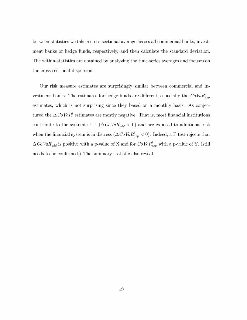
Table 2 provides the estimates of our CoVaR measures that we obtain from using

quantile regressions. Panel A focuses on 19 commercial banks, Panel B on the 9

investment banks and Panl C provides the summary statistic for monthly hedge fund

returns. Estimates are based on weekly equity return data. We opted for a weekly

horizon, since we consider daily tail events are too short, while focusing on monthly

horizon would reduce the number of data points for our tail estimates. Hedge fund

return data are an exception, they are only available at a monthly basis from January

1994 to December 2008.

Table 2 reports institution i�s individual risk, VaRi, the VaR of the whole �nan-

cial sector conditional on institution i being in distress, i.e. the CoVaRiadd , and the

�CoVaRiadd which measures the marginal contribution of institution i to the overall

systemic risk. Recall that �CoVaRiadd re�ects the di¤erence between two value at risk

of the portfolio of the ��nancial universe�. The �nancial universe contains all traded

�nancial institutions, including real estate �nanciers (French�s �Portfolio 49�). Finally,

we report the exposure CoVaRiexp which measures the extent to which institution i is

exposed to a potential systemic event. We report the overall estimates. To obtain the

7There are several papers that compare the self-reported hedge fund returns of di¤erent vendors(see e.g. Agarwal and Naik (2005)), and some research compares the return characteristics of hedgefund indices with the returns of individual funds (Malkiel and Saha (2005)). The literature also inves-tigates biases such as survivorship bias (Brown, Goetzmann, and Ibbotson (1999) and Liang (2000)),termination and self-selection bias (Ackermann, McEnally, and Ravenscraft (1999)), back�lling bias,and illiquidity bias (Asness, Krail, and Liew (2001) and Getmansky, Lo, and Makarov (2004)). Wetake from this literature that hedge fund return indices do not constitute ideal sources of data, butthat their study is useful, and the best that is available. In addition, there is some evidence that theCredit Suisse/Tremont indices appear to be the least a¤ected by various biases (Malkiel and Saha(2005)).

18

between-statistics we take a cross-sectional average across all commercial banks, invest-

ment banks or hedge funds, respectively, and then calculate the standard deviation.

The within-statistics are obtained by analyzing the time-series averages and focuses on

the cross-sectional dispersion.

Our risk measure estimates are surprisingly similar between commercial and in-

vestment banks. The estimates for hedge funds are di¤erent, especially the CoVaRiexp

estimates, which is not surprising since they based on a monthly basis. As conjec-

tured the �CoVaRi estimates are mostly negative. That is, most �nancial institutions

contribute to the systemic risk (�CoVaRiadd < 0) and are exposed to additional risk

when the �nancial system is in distress (�CoVaRiexp < 0). Indeed, a F-test rejects that

�CoVaRiadd is positive with a p-value of X and for CoVaRiexp with a p-value of Y. (still

needs to be con�rmed.) The summary statistic also reveal

19

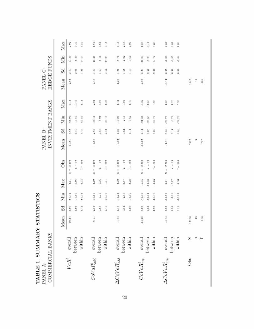
TABLE1,SUMMARYSTATISTICS

PANELA:

PANELB:

PANELC:

COMMERCIALBANKS

INVESTMENTBANKS

HEDGEFUNDS

Mean

SdMin

Max

Obs

Mean

SdMin

Max

Mean

SdMin

Max

VaRi

overall

-10.14

3.95

-60.32

-2.11

N=15200

-11.81

4.68

-68.95

-3.11

-2.84

2.81

-17.39

2.02

between

1.93

-15.69

-6.86

n=19

1.59

-14.89

-10.47

2.09

-6.40

-0.37

within

3.42

-60.13

-0.05

T=800

4.45

-65.86

-1.11

1.99

-14.54

4.87

CoVaRi add

overall

-6.91

2.53

-36.65

-2.10

N=15200

-6.88

2.63

-36.41

-2.01

-7.48

3.87

-25.26

1.66

between

0.68

-7.75

-5.76

n=19

0.85

-8.04

-5.96

1.67

-9.11

-3.61

within

2.45

-36.11

-1.71

T=800

2.51

-35.46

-1.36

3.52

-24.24

-0.44

�CoVaRi add

overall

-1.84

1.18

-13.23

2.90

N=15200

-1.62

1.24

-10.27

1.41

-1.27

1.99

-8.71

4.43

between

0.54

-2.58

-0.57

n=19

0.61

-2.55

-0.97

1.68

-2.92

2.58

within

1.08

-13.05

2.28

T=800

1.11

-9.62

1.45

1.17

-7.62

2.27

CoVaRi exp

overall

-14.48

5.07

-73.15

-5.05

N=15200

-16.12

7.11

-91.33

-4.32

-2.97

3.21

-20.04

1.88

between

2.82

-21.74

-10.98

n=19

4.05

-24.68

-11.60

2.60

-8.24

-0.47

within

4.22

-69.40

-4.46

T=800

6.02

-82.77

0.96

2.03

-14.77

5.30

�CoVaRi exp

overall

-4.34

2.52

-31.75

4.41

N=15200

-4.31

3.89

-29.76

7.00

-0.14

0.95

-6.06

2.82

between

1.55

-7.91

-2.17

n=19

3.17

-9.79

1.26

0.90

-2.55

0.81

within

2.11

-32.03

4.90

T=800

2.58

-24.29

5.92

0.40

-3.64

1.88

Obs

N15200

6902

1845

n19

911

T500

767

168

20

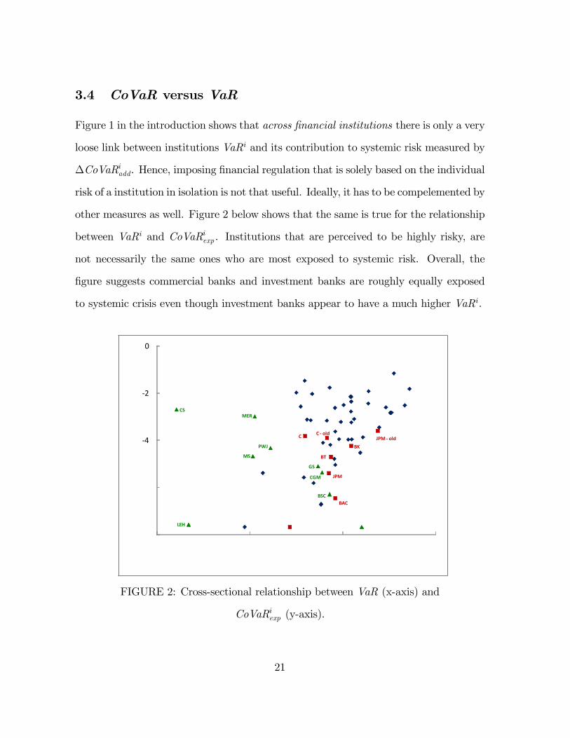
3.4 CoVaR versus VaR

Figure 1 in the introduction shows that across �nancial institutions there is only a very

loose link between institutions VaRi and its contribution to systemic risk measured by

�CoVaRiadd. Hence, imposing �nancial regulation that is solely based on the individual

risk of a institution in isolation is not that useful. Ideally, it has to be compelemented by

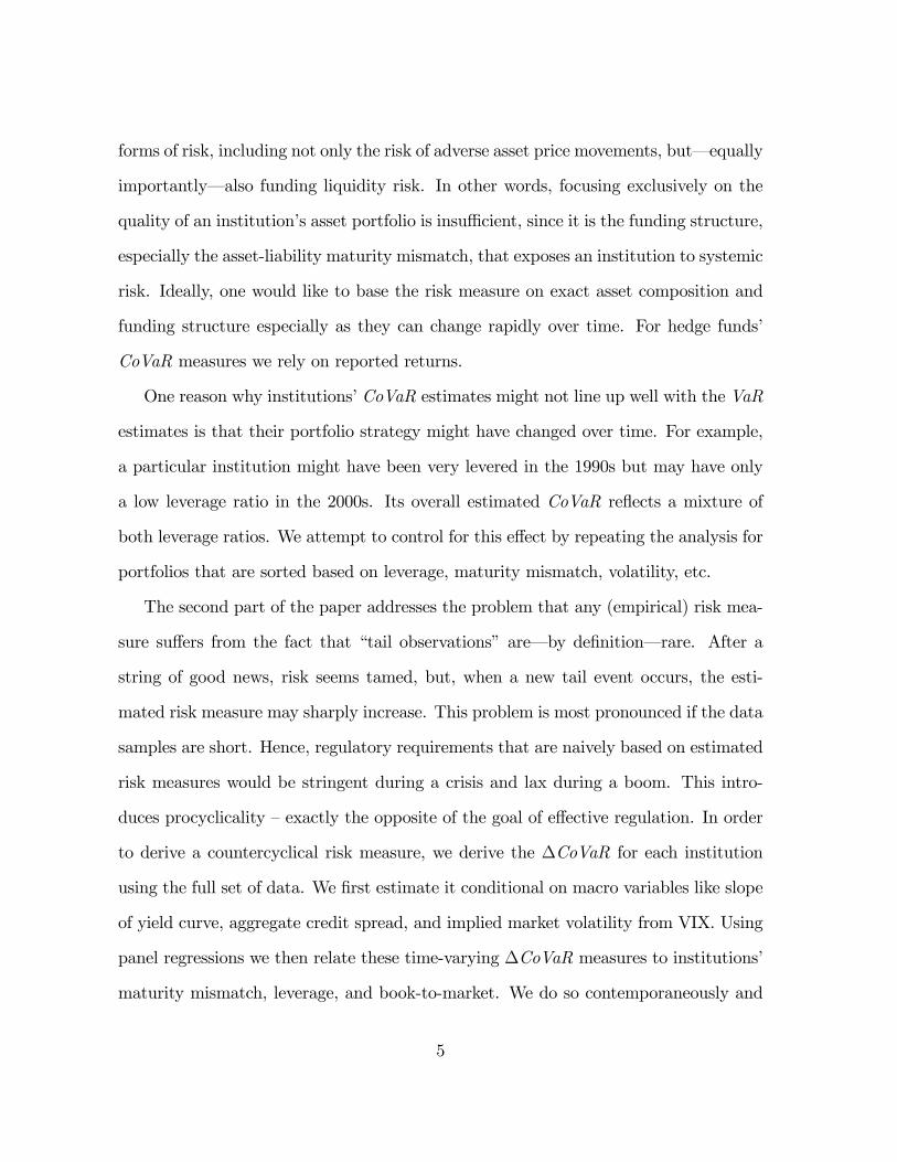
other measures as well. Figure 2 below shows that the same is true for the relationship

between VaRi and CoVaRiexp . Institutions that are perceived to be highly risky, are

not necessarily the same ones who are most exposed to systemic risk. Overall, the

�gure suggests commercial banks and investment banks are roughly equally exposed

to systemic crisis even though investment banks appear to have a much higher VaRi.

­8

­6

­4

­2

0

­21 ­16 ­11 ­6

∆CoVaR

i exp

VaRi

Portfolios Commercial Banks Investment Banks

BSC

MER

LEH

MS

C

JPM

BAC

GS

JPM ­ oldC ­ old

CS

PWJ

CGM

BK

BT

FIGURE 2: Cross-sectional relationship between VaR (x-axis) and

CoVaRiexp (y-axis).

21

The disconnect between VaR and CoVaR in the cross-section is in sharp contrast

to the close link in the time series. Figure 3, Panel A and B show for �CoVaRadd;t

and CoVaRexp ;t, respectively, that at times when the institution�s risk (in isolation),

measured by VaRt, is high the co-risk measures is also high.

­4

­3

­2

­1

0

­21 ­18 ­15 ­12 ­9 ­6 ­3 0

∆CoVaR

i add

VaRi

­8

­6

­4

­2

0

­20 ­16 ­12 ­8 ­4

∆CoVaR

i exp

VaRi

FIGURE 3: Time-series relationship between VaRt (x-axis) and �CoVaRadd;t (y-axis)

in Panel A and between VaRt and �CoVaRexp ;t in Panel B.

22

3.5 Time-varying CoVaR

To capture time-variation of risk measures we relate them to macro factors, described

in Section 2. More speci�cally, we quantile regress the weekly returns on on these macro

variables. Since institution�s investment and funding strategy might have changed over

time, we repeat the analysis for portfolios that are sorted as desribed above. We run

this regressions for each institution separately. Table 2 reportst the (equally-weighted)

average coe¢ cients across all institutions (in Panel A) and across all portfolios (in Panel

B). Recall portfolios are sorted into quintiles according to matuirty mismatch, leverage,

cash to assets, book to market, and equity volatility. The number in paratheses reports

the average t-statistic. The second half of the table reports the average coe¢ cients for

a di¤erent speci�cation. In it, we use the average leverage, maturity mismatch and

book-to-market ratio as variable. This alternative speci�cation will serve as a useful

robustness check later, when we regress risk measures on institution speci�c leverage

etc.

23

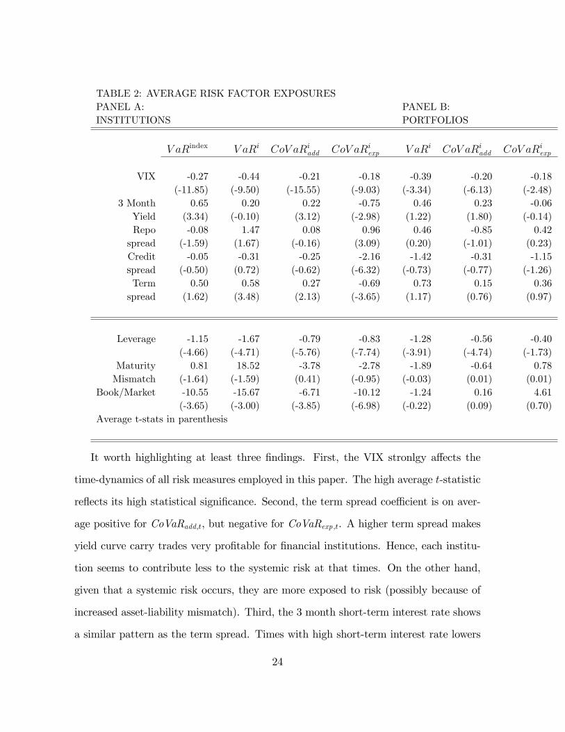
TABLE 2: AVERAGE RISK FACTOR EXPOSURESPANEL A: PANEL B:INSTITUTIONS PORTFOLIOS

V aRindex V aRi CoV aRiadd CoV aRiexp V aRi CoV aRiadd CoV aRiexp

VIX -0.27 -0.44 -0.21 -0.18 -0.39 -0.20 -0.18(-11.85) (-9.50) (-15.55) (-9.03) (-3.34) (-6.13) (-2.48)

3 Month 0.65 0.20 0.22 -0.75 0.46 0.23 -0.06Yield (3.34) (-0.10) (3.12) (-2.98) (1.22) (1.80) (-0.14)Repo -0.08 1.47 0.08 0.96 0.46 -0.85 0.42spread (-1.59) (1.67) (-0.16) (3.09) (0.20) (-1.01) (0.23)Credit -0.05 -0.31 -0.25 -2.16 -1.42 -0.31 -1.15spread (-0.50) (0.72) (-0.62) (-6.32) (-0.73) (-0.77) (-1.26)Term 0.50 0.58 0.27 -0.69 0.73 0.15 0.36spread (1.62) (3.48) (2.13) (-3.65) (1.17) (0.76) (0.97)

Leverage -1.15 -1.67 -0.79 -0.83 -1.28 -0.56 -0.40(-4.66) (-4.71) (-5.76) (-7.74) (-3.91) (-4.74) (-1.73)

Maturity 0.81 18.52 -3.78 -2.78 -1.89 -0.64 0.78Mismatch (-1.64) (-1.59) (0.41) (-0.95) (-0.03) (0.01) (0.01)

Book/Market -10.55 -15.67 -6.71 -10.12 -1.24 0.16 4.61(-3.65) (-3.00) (-3.85) (-6.98) (-0.22) (0.09) (0.70)

Average t-stats in parenthesis

It worth highlighting at least three �ndings. First, the VIX stronlgy a¤ects the

time-dynamics of all risk measures employed in this paper. The high average t-statistic

re�ects its high statistical signi�cance. Second, the term spread coe¢ cient is on aver-

age positive for CoVaRadd;t, but negative for CoVaRexp ;t. A higher term spread makes

yield curve carry trades very pro�table for �nancial institutions. Hence, each institu-

tion seems to contribute less to the systemic risk at that times. On the other hand,

given that a systemic risk occurs, they are more exposed to risk (possibly because of

increased asset-liability mismatch). Third, the 3 month short-term interest rate shows

a similar pattern as the term spread. Times with high short-term interest rate lowers

24

the contribution CoVaRadd;t.

4 CoVaR and Institutions�Characteristics

As explained in Section 2, (time-varying) tail risk measure estimates can depend on

few observations. We therefore try to relate them to variables that are more readily

observable. In the next subsection we do so by relating the risk measure to maturity

mismatch, leverage, book to market and institution�s relative size. In the subsequent

subsection, we show that these variables help us to predict future tail co-risk mea-

sures. Regulators and practioners who have additional sources of data can �nd better

explanatory variables on which �nancial regulation and internal control can be based.

Since most of these variables are only available at a quarterly basis, we aggreagte

weekly CoVaR measures to quarterly CoVaRs by taking the average of the weekly

CoVaR within the same quarter.

25

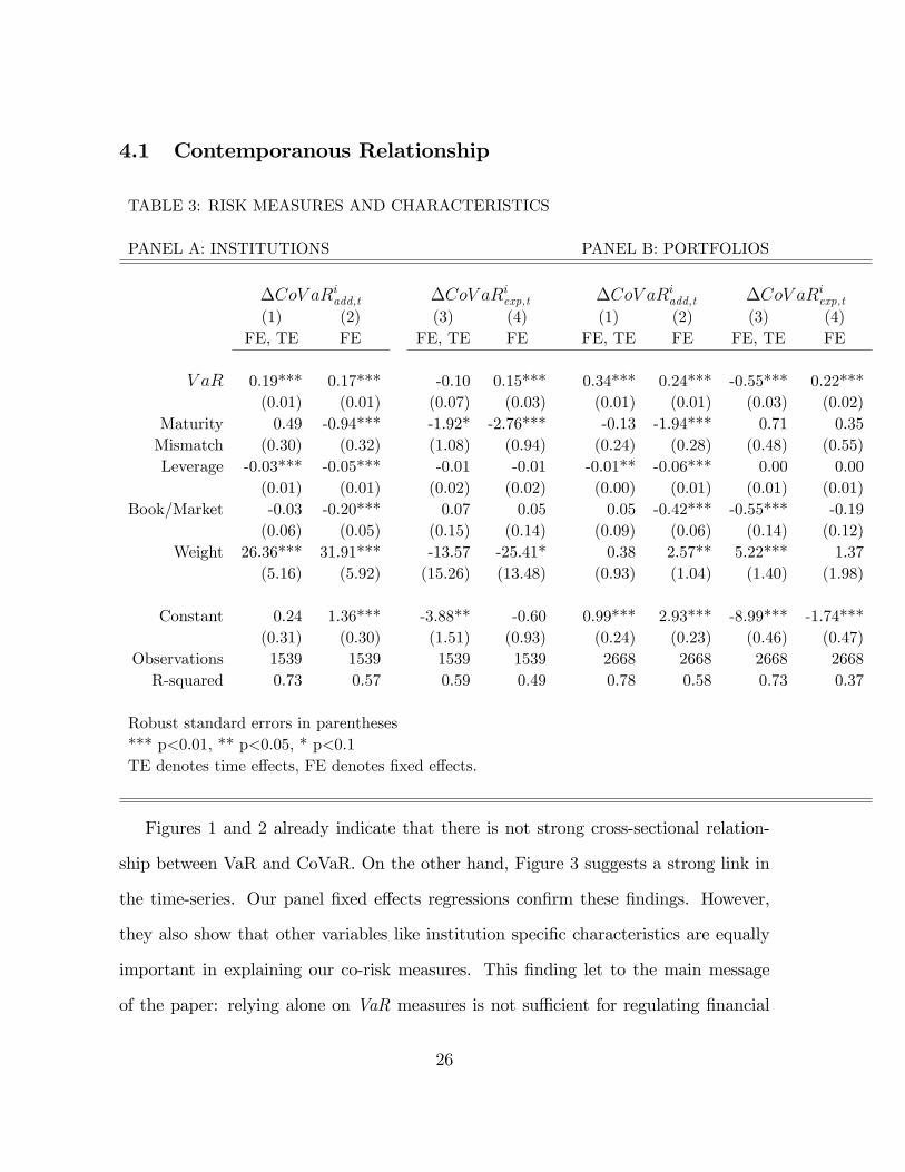
4.1 Contemporanous Relationship

TABLE 3: RISK MEASURES AND CHARACTERISTICS

PANEL A: INSTITUTIONS PANEL B: PORTFOLIOS

�CoV aRiadd,t �CoV aRiexp,t �CoV aRiadd,t �CoV aRiexp,t(1) (2) (3) (4) (1) (2) (3) (4)

FE, TE FE FE, TE FE FE, TE FE FE, TE FE

V aR 0.19*** 0.17*** -0.10 0.15*** 0.34*** 0.24*** -0.55*** 0.22***(0.01) (0.01) (0.07) (0.03) (0.01) (0.01) (0.03) (0.02)

Maturity 0.49 -0.94*** -1.92* -2.76*** -0.13 -1.94*** 0.71 0.35Mismatch (0.30) (0.32) (1.08) (0.94) (0.24) (0.28) (0.48) (0.55)Leverage -0.03*** -0.05*** -0.01 -0.01 -0.01** -0.06*** 0.00 0.00

(0.01) (0.01) (0.02) (0.02) (0.00) (0.01) (0.01) (0.01)Book/Market -0.03 -0.20*** 0.07 0.05 0.05 -0.42*** -0.55*** -0.19

(0.06) (0.05) (0.15) (0.14) (0.09) (0.06) (0.14) (0.12)Weight 26.36*** 31.91*** -13.57 -25.41* 0.38 2.57** 5.22*** 1.37

(5.16) (5.92) (15.26) (13.48) (0.93) (1.04) (1.40) (1.98)

Constant 0.24 1.36*** -3.88** -0.60 0.99*** 2.93*** -8.99*** -1.74***(0.31) (0.30) (1.51) (0.93) (0.24) (0.23) (0.46) (0.47)

Observations 1539 1539 1539 1539 2668 2668 2668 2668R-squared 0.73 0.57 0.59 0.49 0.78 0.58 0.73 0.37

Robust standard errors in parentheses*** p<0.01, ** p<0.05, * p<0.1TE denotes time e¤ects, FE denotes �xed e¤ects.

Figures 1 and 2 already indicate that there is not strong cross-sectional relation-

ship between VaR and CoVaR. On the other hand, Figure 3 suggests a strong link in

the time-series. Our panel �xed e¤ects regressions con�rm these �ndings. However,

they also show that other variables like institution speci�c characteristics are equally

important in explaining our co-risk measures. This �nding let to the main message

of the paper: relying alone on VaR measures is not su¢ cient for regulating �nancial

26

institutions. Even though our funding liquidity measures are not very precise, they

add valuable inforamtion and insight in analyzing institutions� contribution to sys-

temic risk. More precise funding liquidity data would provide even a better guidance.

Finally, it is worth mentioning that for �CoV aRiexp,t the institutions�VaRi is not even

signi�cant in the regression with �xed and time e¤ects.

4.2 Predictive Relationship

Regulation is only countercyclical if it is tight during booms, i.e. before risk measures

increase. Estimated risk measures often only increase at the onset of the crisis. Hence,

in this subsection we try to identify variables which help to predict future CoVaR mea-

sures. Given our limited data source, we focus on the same institutions�characterstics

as before.

27

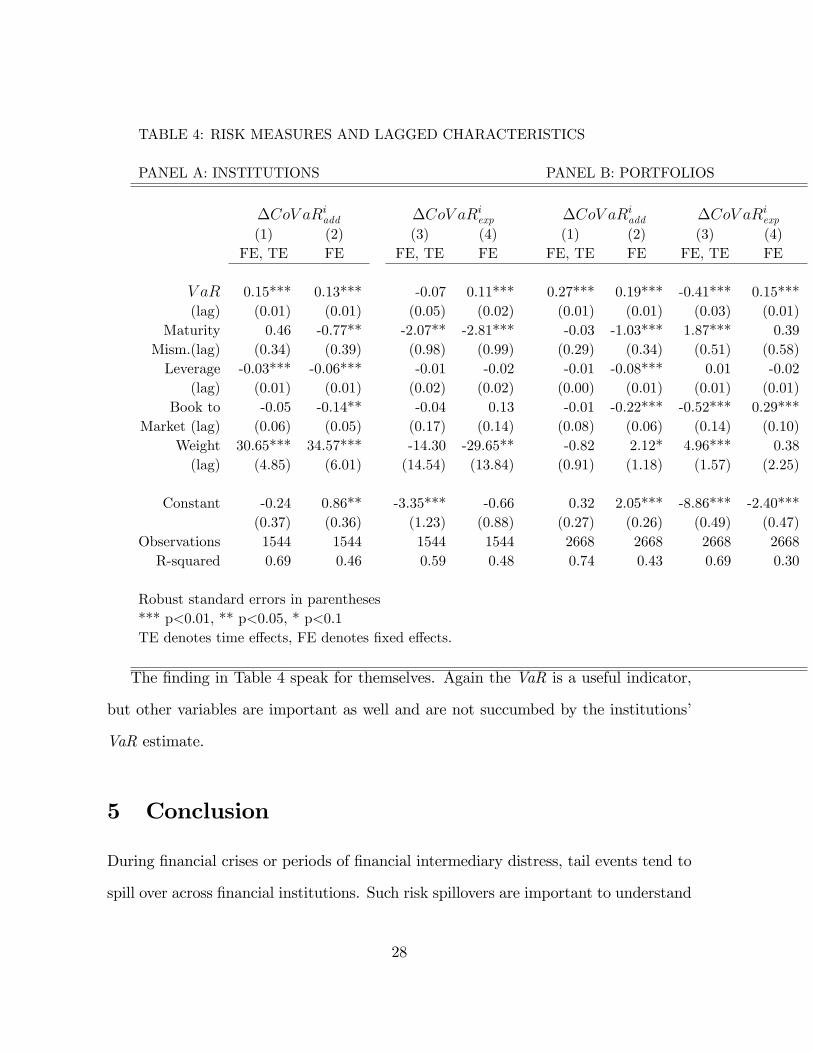
TABLE 4: RISK MEASURES AND LAGGED CHARACTERISTICS

PANEL A: INSTITUTIONS PANEL B: PORTFOLIOS

�CoV aRiadd �CoV aRiexp �CoV aRiadd �CoV aRiexp(1) (2) (3) (4) (1) (2) (3) (4)

FE, TE FE FE, TE FE FE, TE FE FE, TE FE

V aR 0.15*** 0.13*** -0.07 0.11*** 0.27*** 0.19*** -0.41*** 0.15***(lag) (0.01) (0.01) (0.05) (0.02) (0.01) (0.01) (0.03) (0.01)

Maturity 0.46 -0.77** -2.07** -2.81*** -0.03 -1.03*** 1.87*** 0.39Mism.(lag) (0.34) (0.39) (0.98) (0.99) (0.29) (0.34) (0.51) (0.58)Leverage -0.03*** -0.06*** -0.01 -0.02 -0.01 -0.08*** 0.01 -0.02

(lag) (0.01) (0.01) (0.02) (0.02) (0.00) (0.01) (0.01) (0.01)Book to -0.05 -0.14** -0.04 0.13 -0.01 -0.22*** -0.52*** 0.29***

Market (lag) (0.06) (0.05) (0.17) (0.14) (0.08) (0.06) (0.14) (0.10)Weight 30.65*** 34.57*** -14.30 -29.65** -0.82 2.12* 4.96*** 0.38(lag) (4.85) (6.01) (14.54) (13.84) (0.91) (1.18) (1.57) (2.25)

Constant -0.24 0.86** -3.35*** -0.66 0.32 2.05*** -8.86*** -2.40***(0.37) (0.36) (1.23) (0.88) (0.27) (0.26) (0.49) (0.47)

Observations 1544 1544 1544 1544 2668 2668 2668 2668R-squared 0.69 0.46 0.59 0.48 0.74 0.43 0.69 0.30

Robust standard errors in parentheses*** p<0.01, ** p<0.05, * p<0.1TE denotes time e¤ects, FE denotes �xed e¤ects.

The �nding in Table 4 speak for themselves. Again the VaR is a useful indicator,

but other variables are important as well and are not succumbed by the institutions�

VaR estimate.

5 Conclusion

During �nancial crises or periods of �nancial intermediary distress, tail events tend to

spill over across �nancial institutions. Such risk spillovers are important to understand

28

for portfolio managers, risk managers, and supervisors of �nancial institutions. The

ability to monitor and potentially hedge risk spillovers can help to optimize portfolio

performance, to set risk limits and margins, and to adequately regulate institutions.

We �nd statistically and economically signi�cant risk spillovers across institutions.

The �nancial market crisis of 2007-2009 has underscored fundamental problems in

the current regulatory set-up. When regulatory capital and margins are set relative

to VaRs, forced unwinding of one institution tends to increase market volatility, thus

making it more likely that other institutions are forced to unwind and delever as well. In

equilibrium, such unwinding gives rise to a margin/haircut spiral triggering an adverse

feedback loop. An economic theory of such ampli�cation mechanisms are provided

by Brunnermeier and Pedersen (2009) and Adrian and Shin (2009). These �adverse

feedback loops�were discussed by the Federal Open Market Committe in March 2008,

and motivated Federal Reserve Chairman Ben Bernanke to call for regulatory reform.8

Our CoVaR measure provides a potential remedy for the margin spiral, as the measure

takes the volatility spillovers which give rise to adverse feedback loops explicitly into

account. We propose to require institutions to hold capital not only against their

VaR, but also against their CoVaR. �Crowded trades�such as the on-the-run/o¤-the-

run trades that preceded the LTCM crisis, or the short-�nancials/long-oil trade of the

spring of 2008, would be penalized by capital requirements.

For risk monitoring purposes, CoVaR is a parsimonious measure for the potential of

systemic �nancial risk. Institutions that monitor systemic risk� for example, the Fed-

eral Reserve, other central banks around the world, the International Monetary Fund,

and the Bank for International Settlement� have traditionally followed the evolution

of VaRs of the �nancial sector. These institutions have also developed measures of sys-

8See http://www.federalreserve.gov/monetarypolicy/fomcminutes20080318.htm.and http://www.federalreserve.gov/newsevents/speech/bernanke20080822a.htm.

29

temic risk based on time varying second moments, estimates of exposures to di¤erent

risk factors, and �nancial system tail risk measures. The advantage of using CoVaR is

that it is tightly linked to VaR, the predominant risk measure.

30

A Appendix: Quantile Regressions

This appendix is a short introduction to quantile regressions in the context of a linear

factor model. Suppose that returns Rt have the following (linear) factor structure:

Rt = 0 +Xt 1 + ( 2 +Xt 3) "t (4)

where Xt is a vector of risk factors. The error term "t is assumed to be i.i.d. with

zero mean and unit variance and is independent of Xt so that E ["tjXt] = 0. Returns

are generated by a process of the �location-scale" family, so that both the conditional

expected return E [RtjXt] = 0 +Xt 1 and the conditional volatility V olt�1 [RtjXt] =

( 2 +Xt 3) depend on a set of factors. The coe¢ cients 0 and 1 can be estimated

consistently via OLS:9

0 = �OLS (5)

1 = �OLS (6)

We denote the cumulative distribution function (cdf) of " by F" ("), and the inverse

cdf by F�1" (q) for percentile q. It follows immediately that the inverse cdf of Rt is:

F�1Rt (qjXt) = 0 +Xt 1 + ( 2 +Xt 3)F�1" (q) (7)

= � (q) +Xt� (q)

9The volatility coe¢ ents 2 and 3 can be estimated using a stochastic volatility or GARCH modelif distributional assumptions about " are made, or via GMM. Below, we will describe how to estimate 2 and 3 using quantile regessions, which do not rely on a speci�c distribution function of ".

31

where

� (q) = 0 + 2F�1" (q) (8)

� (q) = 1 + 3F�1" (q) (9)

with quantiles q 2 (0; 1). We also call F�1Rt (qjXt) the conditional quantile function and

denote it by QRt (qjXt). From the de�nition of VaR:

VaRqjXt = infVaRq

fPr (Rt � VaRqjXt) � qg (10)

follows directly that

VaRqjXt = QRt (qjXt) (11)

the q-VaR in returns conditional on Xt coincides with conditional quantile function

QRt (qjXt). Typically, we are interested in values of q close to 0, or particularly q = 1%.

Note that by multiplying the (absolute value of the) VaR in return space the by hedge

fund capitalization gives the VaR in terms of dollars.

We can estimate the quantile function via quantile regressions:

��q; �q

�= argmin

�q ;�q

Xt

�q�Rt � �q �Xt�q

�with �q (u) = (q � Iu�0)u (12)

See Koenker and Bassett (1978), Koenker and Bassett (1978), and Chernozhukov and

Umantsev (2001).

32

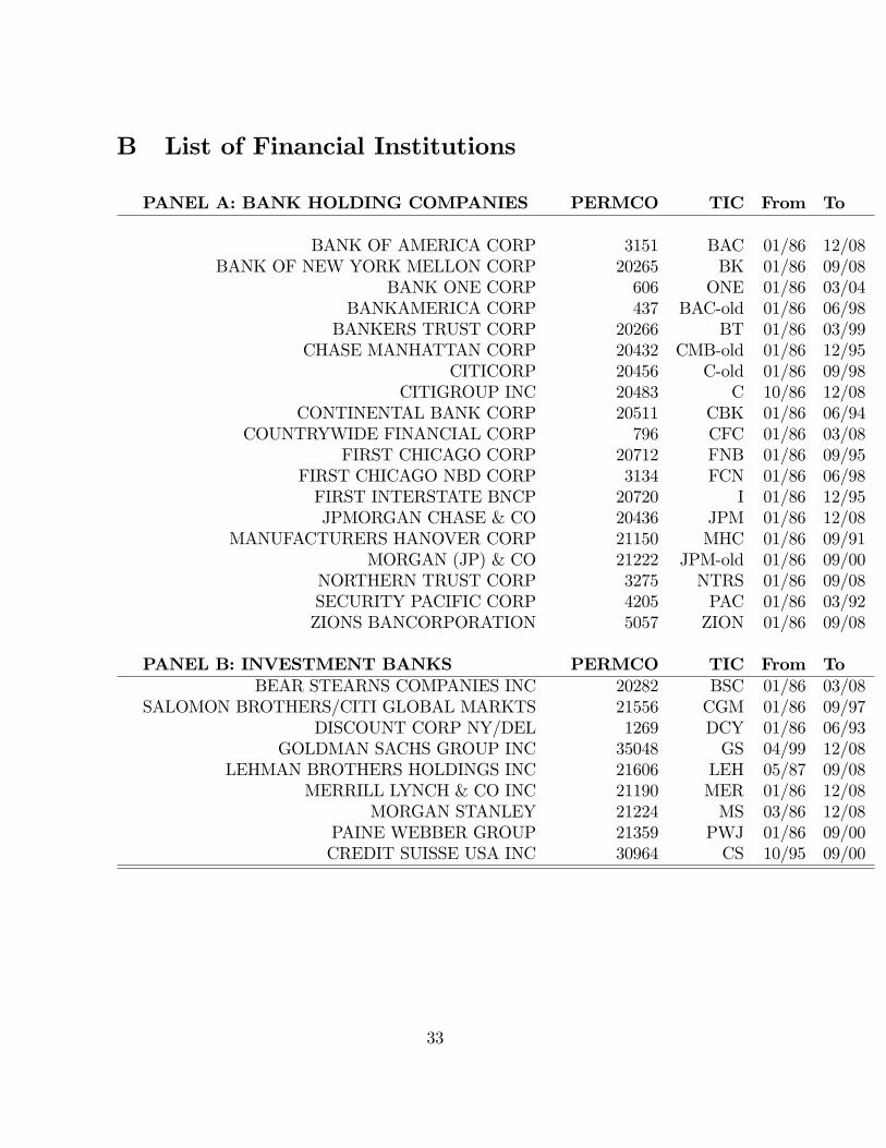
B List of Financial Institutions

PANEL A: BANK HOLDING COMPANIES PERMCO TIC From To

BANK OF AMERICA CORP 3151 BAC 01/86 12/08BANK OF NEW YORK MELLON CORP 20265 BK 01/86 09/08

BANK ONE CORP 606 ONE 01/86 03/04BANKAMERICA CORP 437 BAC-old 01/86 06/98

BANKERS TRUST CORP 20266 BT 01/86 03/99CHASE MANHATTAN CORP 20432 CMB-old 01/86 12/95

CITICORP 20456 C-old 01/86 09/98CITIGROUP INC 20483 C 10/86 12/08

CONTINENTAL BANK CORP 20511 CBK 01/86 06/94COUNTRYWIDE FINANCIAL CORP 796 CFC 01/86 03/08

FIRST CHICAGO CORP 20712 FNB 01/86 09/95FIRST CHICAGO NBD CORP 3134 FCN 01/86 06/98FIRST INTERSTATE BNCP 20720 I 01/86 12/95JPMORGAN CHASE & CO 20436 JPM 01/86 12/08

MANUFACTURERS HANOVER CORP 21150 MHC 01/86 09/91MORGAN (JP) & CO 21222 JPM-old 01/86 09/00

NORTHERN TRUST CORP 3275 NTRS 01/86 09/08SECURITY PACIFIC CORP 4205 PAC 01/86 03/92ZIONS BANCORPORATION 5057 ZION 01/86 09/08

PANEL B: INVESTMENT BANKS PERMCO TIC From ToBEAR STEARNS COMPANIES INC 20282 BSC 01/86 03/08

SALOMON BROTHERS/CITI GLOBAL MARKTS 21556 CGM 01/86 09/97DISCOUNT CORP NY/DEL 1269 DCY 01/86 06/93

GOLDMAN SACHS GROUP INC 35048 GS 04/99 12/08LEHMAN BROTHERS HOLDINGS INC 21606 LEH 05/87 09/08

MERRILL LYNCH & CO INC 21190 MER 01/86 12/08MORGAN STANLEY 21224 MS 03/86 12/08

PAINE WEBBER GROUP 21359 PWJ 01/86 09/00CREDIT SUISSE USA INC 30964 CS 10/95 09/00

33

References

Ackermann, C., R. McEnally, and D. Ravenscraft, 1999, �The Performance of HedgeFunds: Risk, Return, and Incentives,�Journal of Finance, 54(3), 833�874.

Adrian, T., 2007, �Measuring Risk in the Hedge Fund Sector,� Current Issues inEconomics and Finance by the Federal Reserve Bank of New York, 13(3), 1�7.

Adrian, T., and H. S. Shin, 2009, �Financial Intermediary Leverage and Value-at-Risk,�Federal Reserve Bank of New York Sta¤ Reports, 338.

Agarwal, V., and N. Y. Naik, 2004, �Risk and Portfolio Decisions Involving HedgeFunds,�Review of Financial Studies, 17(1), 63�98.

, 2005, �Hedge Funds,�in Foundations and Trends in Finance, ed. by L. Jaeger.vol. 1.

Asness, C. S., R. Krail, and J. M. Liew, 2001, �Do Hedge Funds Hedge?,�Journal ofPortfolio Management, 28(1), 6�19.

Barnes, M. L., and A. W. Hughes, 2002, �A Quantile Regression Analysis of the CrossSection of Stock Market Returns,�Working Paper, Federal Reserve Bank of Boston.

Bassett, G. W., and H.-L. Chen, 2001, �Portfolio Style: Return-based AttributionUsing Quantile Regression,�Empirical Economics, 26(1), 293�305.

Bassett, G. W., and R. Koenker, 1978, �Asymptotic Theory of Least Absolute ErrorRegression,�Journal of the American Statistical Association, 73(363), 618�622.

Bondarenko, O., 2004, �Market Price of Variance Risk and Performance of HedgeFunds,�Working Paper, University of Illinois at Chicago.

Boyson, N. M., C. W. Stahel, and R. M. Stulz, 2006, �Is There Hedge Fund Conta-gion?,�Working Paper, Ohio State University.

Brady, N. F., 1988, �Report of the Presidential Task Force on Market Mechanisms,�U.S. Government Printing O¢ ce.

Brown, S. J., W. N. Goetzmann, and R. G. Ibbotson, 1999, �O¤shore Hedge Funds:Survival and Performance 1989-1995,�Journal of Business, 72(1), 91�117.

Brunnermeier, M. K., 2009, �Deciphering the 2007-0? Liquidity and Credit Crunch,�Journal of Economic Perspectives, (forthcoming).

34

Brunnermeier, M. K., A. Crocket, C. Goodhart, A. Perssaud, and H. Shin, 2009, TheFundamental Principals of Financial Regulation: 11th Geneva Report on the WorldEconomy.

Brunnermeier, M. K., and S. Nagel, 2004, �Hedge Funds and the Technology Bubble,�Journal of Finance, 59(5), 2013�2040.

Brunnermeier, M. K., and L. H. Pedersen, 2009, �Market Liquidity and Funding Liq-uidity,�Review of Financial Studies (forthcoming).

Campbell, J. Y., 1987, �Stock Returns and the Term Structure,�Journal of FinancialEconomics, 18(2), 373�399.

Chan, N., M. Getmansky, S. Haas, and A. W. Lo, 2006, �Systemic Risk and HedgeFunds,� in The Risks of Financial Institutions and the Financial Sector, ed. byM. Carey, and R. M. Stulz. The University of Chicago Press: Chicago, IL.

Chernozhukov, V., and L. Umantsev, 2001, �Conditional Value-at-Risk: Aspects ofModeling and Estimation,�Empirical Economics, 26(1), 271�292.

Claessens, S., and K. Forbes, 2001, International Financial Contagion. Springer: NewYork.

Danielsson, J., and C. G. de Vries, 2000, �Value-at-Risk and Extreme Returns,�An-nales d�Economie et de Statistique, 60.

Engle, R. F., and S. Manganelli, 2004, �CAViaR: Conditional Autoregressive Value atRisk by Regression Quantiles,�Journal of Business and Economic Satistics, 23(4).

Estrella, A., and G. A. Hardouvelis, 1991, �The Term Structure as a Pedictor of RealEconomic Activity,�Journal of Finance, 46(2), 555�567.

Fama, E. F., and K. R. French, 1989, �Business Conditions and Expected Returns onStocks and Bonds,�Journal of Financial Economics, 25(1), 23�49.

Forbes, K. J., and R. Rigobon, 2002, �No Contagion, Only Interdependence: MeasuringStock Market Comovements,�Journal of Finance, 57(5), 2223�2261.

Fung, W., D. A. Hsieh, N. Y. Naik, and T. Ramadorai, 2008, �Hedge Funds: Perfor-mance, Risk and Capital Formation,�Journal of Finance (forthcoming).

Getmansky, M., A. W. Lo, and I. Makarov, 2004, �An Econometric Model of SerialCorrelation and Illiquidity in Hedge Fund Returns,�Journal of Financial Economics,74(3), 529�609.

35

Hamao, Y., R. W. Masulis, and V. K. Ng, 1990, �Correlations in Price Changes andVolatility Across International Stock Markets,�Review of Financial Studies, 3.

Hartman, P., S. Straetmans, and C. G. de Vries, 2004, �Asset Market Linkages in CrisisPeriods,�Review of Economics and Statistics, 86(1), 313�326.

Jorion, P., 2006, �Value at Risk,�McGraw-Hill, 3rd edn.

King, M. A., and S. Wadhwani, 1990, �Transmission of Volatility Between Stock Mar-kets,�Review of Financial Studies, 3(1), 5�33.

Koenker, R., 2005, Quantile Regression. Cambridge University Press: Cambridge, UK.

Koenker, R., and G. W. Bassett, 1978, �Regression Quantiles,�Econometrica, 46(1),33�50.

Kyle, A. S., and W. Xiong, 2001, �Contagion as a Wealth E¤ect,�Journal of Finance,56(4), 1401�1440.

Liang, B., 2000, �Hedge Funds: The Living and the Dead,�Journal of Financial andQuantitative Analysis, 35(3), 309�326.

Ma, L., and L. Pohlman, 2005, �Return Forecasts and Optimal Portfolio Construction:A Quantile Regression Approach,�SSRN Working Paper 880478.

Malkiel, B. G., and A. Saha, 2005, �Hedge Funds: Risk and Return,�Financial Ana-lysts Journal, 61(6), 80�88.

Rossi, G. D., and A. Harvey, 2007, �Quantiles, Expectiles and Splines,�Working Paper,Cambridge University, UK.

Rubin, R. E., A. Greenspan, A. Levitt, and B. Born, 1999, �Hedge Funds, Leverage,and the Lessons of Long-Term Capital Management,� Report of The President�sWorking Group on Financial Markets.

36