Embed Size (px)
Citation preview

Tonini et al.: Invasive Termite Spread 1
Simulation 2
3
Journal of Environmental Entomology: 4
Population Ecology 5
6
7
8
Francesco Tonini 9
University of Florida, Fort Lauderdale 10
Research and Education Center, 3205 11
College Avenue, 12
Davie, Florida, 33314, U.S.A. 13
Phone: +1 954-577-6392 14
Fax: +1 954-424-6851 15
Email: [email protected]
17
18
Simulating the Spread of an Invasive Termite in an Urban Environment Using a Stochastic 19
Individual-Based Model 20
21
Francesco Tonini,1 Hartwig H. Hochmair,1 Rudolf H. Scheffrahn,1 Donald L. DeAngelis,2 22
23
24
1University of Florida, Fort Lauderdale Research and Education Center, 3205 College Avenue, 25
Davie, Florida, 33314, U.S.A. 26
2Dept. of Biology, University of Miami, PO Box 249118, Coral Gables, FL 33124, U.S.A. 27
28
29
30
31
2
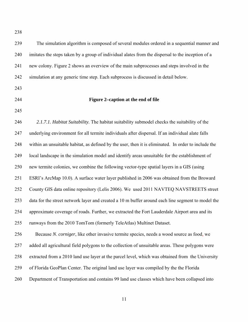
Abstract 32
Invasive termites are destructive insect pests that cause billions of dollars in property damage 33
every year. Termite species can be transported overseas by maritime vessels. However, only if 34
the climatic conditions are suitable will the introduced species flourish. Models predicting the 35
areas of infestation following initial introduction of an invasive species could help regulatory 36
agencies develop successful early detection, quarantine, or eradication efforts. At present, no 37
model has been developed to estimate the geographic spread of a termite infestation from a set of 38
surveyed locations. In the current study, we used actual field data as a starting point, and relevant 39
information on termite species to develop a spatially-explicit stochastic individual-based 40
simulation to predict areas potentially infested by an invasive termite, Nasutitermes corniger 41
(Motschulsky), in Dania Beach, FL. The Monte Carlo technique is used to assess outcome 42
uncertainty. A set of model realizations describing potential areas of infestation were considered 43
in a sensitivity analysis, which showed that the model results had greatest sensitivity to number 44
of alates released from nest, alate survival, maximum pheromone attraction distance between 45
heterosexual pairs, and mean flight distance. Results showed that the areas predicted as infested 46
in all simulation runs of a baseline model cover the spatial extent of all locations recently 47
discovered. The model presented in this study could be applied to any invasive termite species 48
after proper calibration of parameters. The simulation herein can be used by regulatory 49
authorities to define most probable quarantine and survey zones. 50
51
Keywords: Monte Carlo simulation, invasive species, individual-based approach, spatial 52
stochastic simulation, habitat suitability 53
54

3
1. Introduction 55
56
The primary anthropogenic means by which termites are transported between continents and 57
islands is by maritime vessel (Scheffrahn and Crowe 2011). Over a dozen exotic termite species 58
have become established worldwide (Evans 2011), of which six can be found in Florida 59
(Scheffrahn et al. 2002). 60
Termites are destructive insect pests that cause billions of dollars in property damage every 61
year (Edwards and Mill 1986). Once a species is established, the natural dispersal of termite 62
colonies proceeds slowly. Termite colonies typically require 4-6 years to mature, and once the 63
first group of alates (winged reproductives) leaves the colony, they are unable to fly more than a 64
few hundred meters from the parent colony (Husseneder et al. 2006; Messenger and Mullins 65
2005; Mill 1983). Anthropogenic or “vehicular” dispersal is far more rapid and can be measured 66
in km/h. However, such long distance movements lack predictability. Specifically, the nesting 67
core of a termite colony (reproductives, brood, and most foragers) must be moved intact and both 68
a water and food source must be associated with the core during movement (Hochmair and 69
Scheffrahn 2010). 70
The inherent complexity of a physical environment limits the applicability of mathematical 71
models for realistic dispersal modeling of invasive species, and practical predictions are difficult 72
to obtain (Pitt 2008). Analytical methods commonly used to model dispersal in the past and in 73
some cases up to the present include: (i) simple reaction-diffusion models (Fisher 1937), which 74
ignore any spatial interaction between individuals and do not consider single dispersal events; 75
(ii) mixed diffusion-population growth models, which include a per capita growth parameter 76
(Okubo 1980; Skellam 1951) or several demographic variables (Van Den Bosch et al. 1990); and 77

4
(iii) integro-differential equation models, which separate population dynamics and dispersal into 78
two stages (Neubert et al. 1995). More recently, computer-intensive approaches, such as 79
spatially-explicit population models (SEPMs), have been able to incorporate both 80
ecological/biological information at a population level with underlying habitat differences 81
(Wiegand et al. 2004). 82
Computer simulations seek to imitate the dynamics of various real world processes (Steyaert 83
1993) rather than solving sets of equations. Simulation models are either deterministic or 84
stochastic. The first model type gives a fixed output for a given set of input data and model 85
parameters while the second model type includes at least one stochastic process and provides a 86
probabilistic outcome (Law and Kelton 1982). The intrinsic dynamic component of a computer 87
simulation provides the ability to estimate the rate at which an invading species is likely to 88
occupy suitable areas. However, such models may represent a poor choice in cases where 89
established populations are restricted to distinct areas of suitable habitat, since assuming 90
universal dispersal abilities may not reflect the ability of a species to move from a current 91
location to another potentially suitable habitat (Peterson et al. 2002). Whereas simulating the 92
spread of invasive species beyond a decade into the future may decrease the reliability of the 93
model outcome (Pitt et al. 2011), it should be noted that the invasive plant used by Pitt et al. 94
(2011) has a much faster dispersal capacity compared to termites. 95
Individual-based models (IBMs) are able to incorporate several rules describing the 96
interactions between individual units considering each one of them as different, both 97
physiologically and behaviorally (Huston et al. 1988). The complexity of the rules increases with 98
the total number of parameters involved in describing them. However, complexity often comes at 99
the expense of generality, which makes it necessary to select the most appropriate modeling 100

5
approach on a case by case basis. Small spatial scales, such as urban environments, are 101
particulartly suitable for the development of IBMs, because they are complex enough to require 102
simulation but not so large as to be unmanageable for an IBM. Also, IBMs are able to represent 103
individuals explicitly and incorporate biologically relevant rules that have a strong influence on 104
the dynamics of an invasion (Pitt 2008). 105
In this paper, we develop a computer simulation using a spatially-explicit stochastic 106
individual-based modeling approach and use hindcasting in order to predict which areas would 107
have been infested by an arboreal invasive termite, Nasutitermes corniger (Motschulsky), had no 108
eradication plan been implemented at a particular location, Dania Beach, FL. The methodology 109
presented herein is appropriate for more general application, such as predicting the future 110
geographical spread or studying a different termite species after appropriate adjustments in the 111
model paramenters. 112
Individual-based simulations consider the individual organism to be a logical basic unit for 113
modeling ecological phenomena (Grimm and Railsback 2005). We ran each model from 2003, 114
the year in which a first complete survey of infested locations had been conducted over the study 115
area, until 2012. The model outcome is the predicted areas of infestation at any time step, 116
indicating the spatial extent and dynamic evolution of the invasion. Beginning in 2003, local 117
authorities have been trying to eradicate this pest from the original survey area. However, 118
between 2006 and 2011, extended survey procedures had to be stopped due to discontinued 119
funds. A new recent survey conducted in 2012 found newly infested locations in areas not 120
spotted originally and therefore not included in the eradication plan. We believe that state or 121
local regulatory agencies can benefit from a model that predicts the rate and direction of termite 122

6
dispersal, as it would assist them in targeting specific areas for survey, eradication, or quarantine 123
efforts. 124
In the literature, only two computer simulation models have been applied to a termite 125
species: one has been developed to determine per-capita wood consumption rates of termite 126
workers (Morales Ramos and Rojas 2005), while the other explored termite foraging behavior 127
underneath the soil (Lee et al. 2008). To date, no computer simulation models have been 128
published that investigate the geographic spread of a termite infestation from a set of surveyed 129
locations. Unlike some other recently developed spatial simulation models found in the literature 130
for other insects (Carrasco et al. 2010; Pitt 2009) the human-mediated dispersal component is 131
not included because of its unpredictability and lack of calibration data. Although samples 132
collected over the past 10 years do not reflect the true (i.e. natural) expansion of the species, and 133
were collected mainly for the purpose of verifying the success of the eradication effort, it is 134
nevertheless possible to use the newly infested locations (2012) to ground truth our simulation 135
model. 136
We herein describe the parameters and methods used to develop the computer simulation. 137
Results are presented together with a discussion on the relative importance of each biological 138
parameter included in the model, followed by conclusions. 139
140
141
142
143
144
145

7
2. Materials and Methods 146
147
2.1. Model Design 148
149
The simulation algortihm is implemented using a set of R functions (R Development Core 150
Team 2011) and we provide free source code. The model description follows the ODD 151
(Overview, Design concepts, Details) protocol (Grimm et al. 2006; Grimm et al. 2010) in order 152
to make the model's logic as clear as possible. 153
154
2.1.1 Purpose of Model. 155
156
We developed a spatial, stochastic computer simulation with the purpose of gaining a deeper 157
understanding of the rate and direction of a termite invasion by natural means over a realistic 158
landscape, such as an urban environment. In this study, the model is also used to determine how 159
a new invasive species in South Florida, N. corniger, could have expanded from a set of 160
surveyed locations up to the present, if no eradiction plan had been implemented throughout the 161
years. The developed simulation model may assist state or local regulatory agencies in targeting 162
specific areas for survey, eradication, or quarantine efforts. 163
164
2.1.2. Entities, State Variables and Scales. 165
166
The basic entities of the model are individual termite alates (dispersing propagules) and all 167
the individual colonies they are generated from. Both alates and colonies are characterized by 168

8
their continuous spatial location specified in a Cartesian plane coordinate system. Alates are also 169
characterized by their sex (M-F), and colonies by their age (in years). We use a reference spatial 170
grid to represent the distribution of all areas occupied by one or more termite colonies at each 171
time step. The grid is set to an extent of 10 km x 10 km over the urban area of Dania Beach, FL, 172
with a resolution of 100 x 100 meters. We believe that the chosen resolution is suitable for a few 173
reasons such as the uncertainty associated with the precise locations of surveyed 174
colonies/individuals, the approximate maximum extent of a colony’s foraging territory (Collins 175
1981), and because it is a suitable scale of surveillance and pest control management. In order for 176
the simulation to be more realistic, we also consider the local urban environment and exclude 177
areas that are unsuitable for the establishment of a new colony, such as roads, highways, non-178
wooded fields, and water bodies. Each area with wood sources (e.g., buildings, trees, boats, 179
debris, etc.) has potential for colonization. We believe that for the chosen temporal resolution (10 180
years) the choice of a static habitat suitability layer does not introduce any relevant bias in the 181
results. However, should the model be run over a much longer time span, we recommend 182
considering a different strategy. The temporal scale is discrete and one time step represents 1 183
year. The model is run from 2003 (year of the first complete survey of infested locations) to 184
2012. 185
186
2.1.3. Process overview and scheduling. 187
188
Dispersal of alates is the key process in the spread of colonies, and we simulate the dispersal 189
as a single annual event. The consequence may be an increased chance for alates to find a mate 190
and form a new colony. However, this represents a necessary simplification, since typical termite 191

9
dispersal is formed by a major exodus that may be preceded and/or followed by smaller flights, 192
of unknown magnitude and timing. Many termite species initiate dispersal flights in the early 193
stages of the wet season and are triggered by environmental factors (Jones et al. 1988; Martius 194
2003; Nutting 1969). Dispersal flights are the only means by which new colonies can form 195
beyond the foraging territory of the mother colony. Although the model simplifies the temporal 196
scale of the real phenomenon, single massive dispersal flights are common because: (i) alates are 197
less vulnerable as prey, as they can overwhelm predators by large numbers (Nutting 1969); and 198
(ii) there are higher odds of finding and choosing a mate. 199
200
2.1.4. Design Concepts. 201
202
2.1.4.1. Sensing. Dispersing alates (reproductives) can sense and respond to pheremones in 203
order to find potential mates of the opposite sex that have dispersed by chance to the nearby 204
sites. 205
2.1.4.2. Interaction. Male and female alates interact to form new colonies. 206
2.1.4.3. Stochasticity. Both distance and direction of dispersal by alates are determined 207
stochastically from a probability distribution (see Section 2.1.7.4). The sex (male or female) of 208
a particular alate is random. 209
2.1.4.4. Collectives. Individual alates are followed during dispersal, but after a colony is 210
formed by two alates of the opposite sex, the colony is followed as whole rather than at the 211
resolution of individuals. 212
213
2.1.5. Initialization. 214

10
215
Fig. 1 shows a schematic representation of the steps involved for the model initialization. 216
217
Figure 1–caption at the end of file 218
219
At the initial state, i.e. time t=1, the spatial locations of all surveyed termite colonies are stored in 220
a dataset and assigned a random age between 0 and the maximum lifespan decided by the user. 221
The initialization process is the same in all simulation runs. Surveyed colonies can be imported 222
from an external data file containing their geographic coordinates, e.g. recorded with a GPS 223
device. In most cases, the collected samples do not identify different termite colonies, as they are 224
taken opportunistically with the goal of spotting an infestation. Therefore, different termite 225
locations may or may not belong to the same colony. 226
227
2.1.6. Input Data. 228
229
Table 1 shows seven main parameters of the implemented dispersal model and their baseline 230
values, i.e. the values assigned for the baseline simulation, which are based either on related 231
literature findings (see Section 2.3) or the opinion of termite experts. More specific information 232
for the particular location modeled, Dania Beach, FL, is described in Section 3. 233
234
Table 1-end of file 235
236
2.1.7. Submodels. 237
11
238
The simulation algorithm is composed of several modules ordered in a sequential manner and 239
imitates the steps taken by a group of individual alates from the dispersal to the inception of a 240
new colony. Figure 2 shows an overview of the main subprocesses and steps involved in the 241
simulation at any generic time step. Each subprocess is discussed in detail below. 242
243
Figure 2–caption at the end of file 244
245
2.1.7.1. Habitat Suitability. The habitat suitability submodel checks the suitability of the 246
underlying environment for all termite individuals after dispersal. If an individual alate falls 247
within an unsuitable habitat, as defined by the user, then it is eliminated. In order to include the 248
local landscape in the simulation model and identify areas unsuitable for the establishment of 249
new termite colonies, we combine the following vector-type spatial layers in a GIS (using 250
ESRI’s ArcMap 10.0). A surface water layer published in 2006 was obtained from the Broward 251
County GIS data online repository (Lelis 2006). We used 2011 NAVTEQ NAVSTREETS street 252
data for the street network layer and created a 10 m buffer around each line segment to model the 253
approximate coverage of roads. Further, we extracted the Fort Lauderdale Airport area and its 254
runways from the 2010 TomTom (formerly TeleAtlas) Multinet Dataset. 255
Because N. corniger, like other invasive termite species, needs a wood source as food, we 256
added all agricultural field polygons to the collection of unsuitable areas. These polygons were 257
extracted from a 2010 land use layer at the parcel level, which was obtained from the University 258
of Florida GeoPlan Center. The original land use layer was compiled by the the Florida 259
Department of Transportation and contains 99 land use classes which have been collapsed into 260

12
15 classes by the GeoPlan Center (University of Florida Geoplan Center 2010). Using the union 261
overlay operation in ArcMap, we combined all the GIS layers listed above into a single layer 262
denoting unsuitable habitat areas in which colonies are not able to survive. 263
2.1.7.2. Alate Dispersal. The dynamics and speed of termite dispersal by natural means are 264
controlled by several behavioral characteristics affecting the successful creation of new colonies. 265
We identified and included such behavioral characteristics in the form of model parameters to 266
better simulate the real process. A new colony begins with a male-female (i.e. king and queen) 267
couple of unwinged alates building and sealing the nuptial chamber in a proper substrate, usually 268
soil or wood. After a termite colony matures, which requires about 4 years, alates are produced. 269
All alates change their behavior in response to: (i) changes of habitat, i.e. they may fall into an 270
unsuitable patch of land and therefore are not able to find a location to form an incipient colony; 271
(ii) their proximity to a heterosexual mate. Alates do not adjust their behavior over time as a 272
consequence of their experience, since they only serve the purpose of expanding the colony with 273
a one-time flight after which they either die or find a mate and become the king/queen of a new 274
colony. Although they have eyes, alates are probably not able to predict which location will be 275
suitable once in flight. Dispersal flights typically occur at dusk or at night after a light rain and 276
during calm weather conditions. It is known that alates are attracted by lights, as found in mark-277
recapture studies (Messenger and Mullins 2005). Sex pheromones have two main roles: a close-278
range attraction and contact attraction. The former is used to unite sexual partners, the latter is 279
used to maintain the contact during the tandem behavior (Nutting 1969). Alates do not release 280
pheromones during the flight and therefore their flight behavior is not influenced by it. The 281
processes that are modeled assuming they are stochastic, i.e., random, are the flight distance, 282
13
flight direction, and the sex of each individual. The model output is used to spot which areas 283
have been occupied and how often throughout all 100 runs. 284
2.1.7.3. Colony Formation. The colony formation subprocess loops through each grid cell 285
that is occupied by at least two individuals and, subsequently, through each individual. This 286
process is necessary to check if a reproductive is able to find a heterosexual neighbor and form a 287
nuptial pair, where the neighborhood is defined by a circular buffer with the pre-set pheromone 288
attraction radius. If two candidate alates are matched, a new colony is created and assigned 289
spatial coordinates of the mid point between the two individuals. The process stops for a 290
particular grid cell as soon as the maximum density of colonies per hectare is reached. At the end 291
of the present subprocess, if one or more pairs of individuals are matched, new colonies are 292
created and their spatial location is saved. 293
2.1.7.4. Colony Aging and Alate Production. Each time step, the age of every existing colony 294
is increased by one (aging submodel). If this value exceeds the maximum lifespan defined by the 295
user, then the colony is eliminated from the map. After the aging subprocess, alates are generated 296
by each existing colony based on colony age (dispersal subprocess). Older colonies generate 297
more alates, which increase the overall chances for an individual reproductive to find a mate, a 298
suitable nesting site, and a location farther away from the mother colony. The dispersal 299
subprocess also executes the following: (i) random creation of male and female individuals by 300
sampling from a Binomial distribution, Bin(n,p), where n is the number of alates to be generated 301
and p is the probability of drawing a male, (ii) random sampling of flight directions (in radians) 302
from a uniform distribution, Unif[0, 2π], (iii) random sampling of flight distances (Euclidean) 303
from a negative exponential distribution, Exp(λ), with mean 1/λ (where λ = rate), and (iv) 304
14
calculation of new spatial locations X and Y (Easting and Northing) of alates derived from basic 305
trigonometric equations, using both the simulated flight direction and flight distances. 306
2.1.7.5. Updating the Distribution of Colonies on the Landscape. The final subprocess 307
(stacking colonies subprocess) stacks all new colonies created during the previous process 308
(colony formation) with the existing ones in a dataset. Before moving to the next time step, all 309
colonies can be saved to an external shapefile as points and further converted to a geo-referenced 310
raster grid. The raster grid allows us to overlay modeling results from multiple simulations and to 311
compute a final occupancy envelope. At the following time step, new alates are generated which 312
fly out from all mature colonies, i.e., colonies old enough to produce alates. 313
314
2.2. Sensitivity Analysis 315
316
We ran a sensitivity analysis to assess the contribution of each parameter to the model 317
outcome. The uncertainty associated with the outcome of a stochastic simulation was estimated 318
through the Monte Carlo technique and 100 simulation runs. We chose this number as a 319
compromise between short computational time and high precision of confidence intervals around 320
the mean predicted area of infestation. A set of model realizations describing the effect of 321
changes in parameter values on potential areas of infestation were also considered in a sensitivity 322
analysis. 323
324
2.3. Model Parameterization 325
326
15
We used basic data relevant to several termite species in order to parameterize the model. 327
Unfortunately, there is not sufficient data to calibrate the model directly against N. corniger at 328
the Dania Beach site. The age of colonies at the first production of alates, which varies between 329
different termite species, can be derived from related literature studies. Typically, a colony takes 330
four to six years from its creation to reach maturity and start the production of alates (Collins 331
1981). In this paper, we set the baseline value of the age of first production to 4 years. Lifespan 332
estimates are approximations because they only reflect laboratory conditions. Estimated maxima 333
ranged from 15 years old in Macrotermes bellicosus (Keller 1998) to 20 years in 334
Pseudacanthotermes spiniger and P. militaris (Connétable et al. 2012). In this work, we set an 335
age threshold of 20 years, after which a colony dies. 336
The maximum distance of pheromone attraction currently reported is 2.5-3 m by males 337
(Leuthold and Bruinsma 1977). Here, we set the baseline value for the model at 3 meters. 338
The density of termite colonies over a certain patch of land is related to its specific biology, 339
ecology and behavior (Adams and Levings 1987). No specific literature sources studied the 340
density of N. corniger's colonies within an urban environment. However, a study found a density 341
of approximately 7 colonies per hectare in a primary forest in Panama (Thorne 1982), which we 342
use as a baseline value in our model. 343
Literature sources treating the topic of alate predation or alate flight success rate are scant. 344
Both predation and injuries typically occur as alates start leaving the nest (i.e. pre-flight), in 345
flight (bats and birds), and as soon as they alight on the ground or on a tree (i.e. post-flight) to 346
search for a mate. Empirical observation of alates of a different invasive termite species, 347
Cryptotermes brevis, found an approximate survival rate of 1%, excluding predation (Scheffrahn 348
et al. 2001). Factors affecting the outcome and the success of the dispersal flight include 349
16
environmental conditions, number of alates, sex ratio, proportion of alates eaten by predators, 350
and efficiency of the post-flight mating behavior (Noirot 1990; Nutting 1969). A recent field 351
study for two termite species showed that, despite the presence of 40 mature colonies over an 352
area of one hectare producing approximately one million alates every year, no new colonies were 353
found (Connétable et al. 2012). In this paper, we set the baseline value of the overall survival rate 354
to 0.01 (1%). We consider this to be a realistic estimate considering all the aforementioned 355
factors (Scheffrahn, personal communication). 356
Although sex ratios of termite alates are variable, they tend towards parity (Jones et al. 1988). 357
In N. corniger, individual colonies produced alates whose sex ratio was around 1:1 (Darlington 358
1986; Thorne 1983). Therefore, we set the baseline value of the prevalence of male alates in the 359
colony to 0.5 (50%). 360
Field studies aiming to precisely assess the size of an alate crop in individual colonies are 361
rare. Several colonies of N. corniger have been compared and a noticeable variation in 362
production of alates was found. Mature colonies, whose population size ranges between 50,000-363
400,000 individuals, produced 5,000-25,000 alates (Thorne 1983). The production of alates 364
likely depends on factors such as availability of food resources, health of queen(s), colony age, 365
and colony-specific history. All factors are not easily assessed during the short time frame given 366
in field sampling. In another invasive termite, Coptotermes formosanus, the alate production of a 367
single colony was over 68,000. In this case, sex ratio was 1:3 (F:M) (Su and Scheffrahn 1987). 368
In the baseline simulation model, we used a “Low Profile” age-related alate production, defined 369
as follows: (i) no production of alates until a colony reaches 4 years of age, (ii) 1,000 alates 370
between 4 and 9 years of age, (iii) 10,000 alates between 10 and 14 years of age, and (iv) 371
100,000 alates between 15 years and the age at which a colony dies. Opposed to this profile, we 372

17
also defined a “High Profile” scenario, with a greater production of alates at an earlier age: (i) no 373
production of alates until a colony reaches 4 years of age, (ii) 10,000 alates between 4 and 9 374
years of age, (iii) 50,000 alates between 10 and 14 years of age, and (iv) 100,000 alates between 375
15 years and the age at which a colony dies. This alternative scenario is tested in our sensitivity 376
analysis (see Section 4). Although these “profiles” may be an oversimplification, it is likely to 377
match an average magnitude that is otherwise impossible to calibrate with precise empirical data 378
(Scheffrahn personal communication). 379
Termite alates are weak, erratic fliers. On average, alates are capable of flying a few hundred 380
meters on their own (Nutting 1969). Flight distances have not specifically been estimated for N. 381
corniger. However, it is possible to estimate this model parameter based on findings for other 382
termite species. Mark-recapture studies using light traps gave the first empirical measurements of 383
termite flight skills. A maximum distance of 892 m has been recorded for C. formosanus 384
(Messenger and Mullins 2005). In an endemic habitat, alates may fly far enough to ensure that a 385
mixture of different colonies is created with swarm aggregation (Husseneder et al. 2006). 386
However, for an exotic population to spread, alates fly into uncolonized areas lacking 387
conspecifics with which to mate. Recently, a new maximum distance record of about 1.3 km has 388
been recorded by Mullins and Messenger in New Orleans, LA (Mullins, personal 389
communication). Alates of Odontotermes formosanus were capable of flying between 120 and 390
743 m (Hu et al. 2007). Other studies recorded only a few dispersal flights covering about 300 m 391
for termite species belonging to the Termitidae family (Mill 1983), to which N. corniger belongs, 392
or 460 m for C. formosanus (Ikehara 1966). In this study, we decided to sample dispersal flight 393
distances from an exponential distribution. This allows for both short and rare longer dispersal 394
events. In a unique mark-recapture study recently completed in New Orleans, LA, data collected 395
18
for alates of C. formosanus confirmed the “exponential” shape of the empirical histogram 396
derived from several recorded flight distances (Mullins, unpublished data). We estimated the 397
mean of the exponential distribution based on the aforementioned empirical data and literature 398
findings. The baseline value used as a mean dispersal distance for the simulation model was set 399
to 200 m. 400
Two factors that affect alate dispersal distance during the swarm season are wind velocity 401
and light intensity. In most cases, the flight is only initiated if the wind velocity stays below 3.5 402
km/h (Leong et al. 1983). Moreover, termites are extremely prone to injuries, hence windless or 403
low wind conditions are preferred. Given the impossibility of forecasting wind direction, wind 404
speed, and light intensity in a multi-year simulation model, we assume alates can fly in any 405
direction and sample all angles (in radians) from a uniform distribution. Moreover, we are using 406
the present model within an urban environment, where light intensity is quite uniformly 407
distributed and therefore we believe it will not affect the model outcome. 408
409
410
411
412
413
414
415
416
417
418

19
3. Application of Model to Specific Study Area and Data 419
420
N. corniger was first reported in Florida in May 2001, in Dania Beach, Broward County, FL 421
(Scheffrahn et al. 2002). The discovery represents the first record of a non-endemic and land-422
based establishment of a higher termite (Family Termitidae) in the continental U.S. It is likely 423
that the infestation was the result of dockside flights from an infested boat or shipping container, 424
probably a decade before the discovery, but no specific source was identified (Scheffrahn et al. 425
2002). Starting in early 2003, a previously delineated area was targeted for a deliberate 426
eradication campaign of this invasive pest. In January 2003, an area-wide visual survey was 427
conducted for nests, foraging tubes, foraging sites, and debris harboring living N. corniger. 428
However, most N. corniger nest locations were cryptic and even an exhaustive survey is likely to 429
miss some infested locations, especially in the case of young colonies. In 2006, survey work was 430
discontinued due to budget cuts before being re-activated in 2011 (Scheffrahn, unpublished 431
data). 432
Exact sample locations were recorded using a GPS device and later imported into a database. 433
A total area of 200 acres (approximately 81 ha) was surveyed, 20% of which had active 434
infestations. Several epigeal nests of different diameters were found at the base of both live and 435
dead trees, in tree cavities above ground, and foraging tubes extended upward of 10 m on trees 436
and palms (Scheffrahn et al. 2002). The maximum separation between active sites in north-south 437
and east-west direction was approximately 1 km. A newly funded 2011-2012 survey revealed 438
new infested locations. No pest reoccurrence was observed within the areas originally surveyed 439
between 2003 and 2006 (Scheffrahn, unpublished data). 440
20
Fig. 3 shows the known infested area in 2003, with a zoom over the recorded GPS locations 441
of all sampled termites. The total area covers less than 0.25 km2 and consists of commercial, 442
residential, marina, and vacant wooded properties. 443
444
Figure 3–caption at the end of file 445
446
447
448
449
450
451
452
453
454
455
456
457
458
459
460
461
462
463

21
4. Results and Discussion 464
465
The stochastic outcome of 100 computer simulations can be grouped and represented by 466
different occupancy envelopes. A “>0%” occupancy envelope groups all areas predicted as 467
occupied by the model in at least one simulation run. Similarly, a “>=50%” occupancy groups all 468
areas predicted as occupied in at least half of all runs. Finally, the “100%” occupancy envelope 469
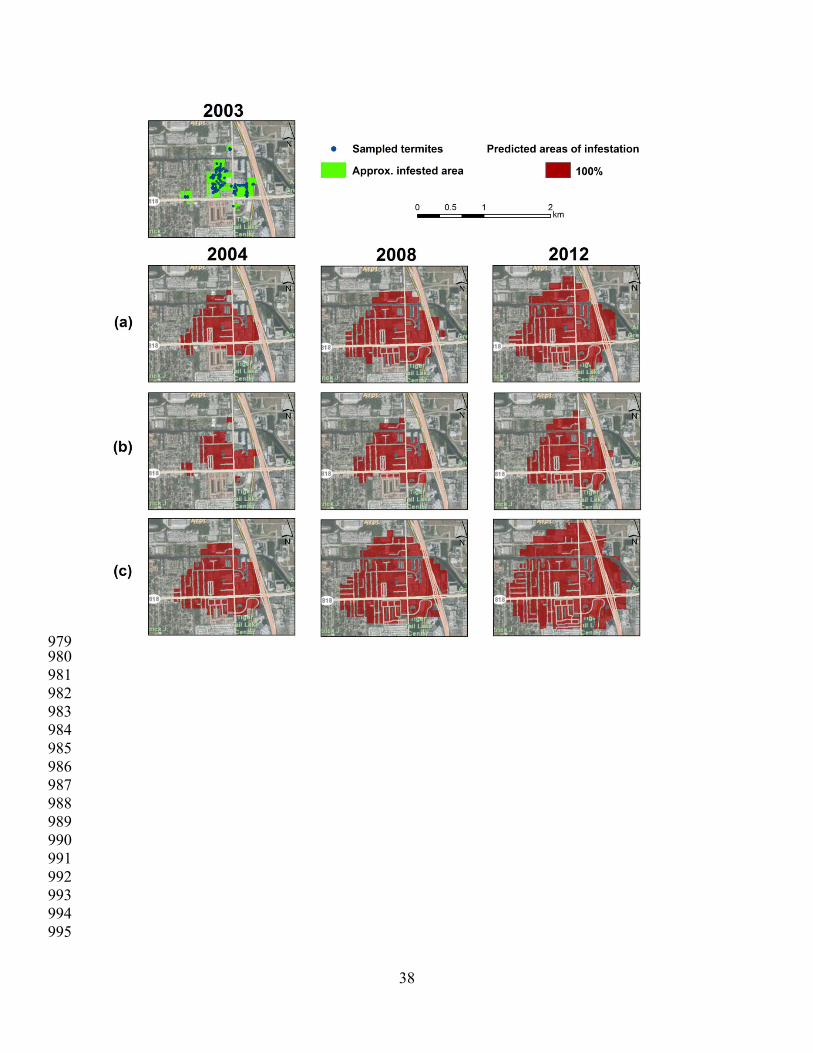
groups areas that are predicted as infested in all runs. Fig. 4 shows a snapshot of the spatial 470
expansion of N. corniger through time as predicted by the baseline simulation model, with color 471
coding to represent the different occupancy envelopes. 472
473
Figure4–caption at the end of file 474
475
Between 2003 and 2004 in the model there was a larger expansion in the areas surrounding the 476
first surveyed locations compared to all other time frames. There are two reasons for that: (1) 477
alates fly in all directions and therefore, if the habitat is suitable, fill in all the voids; (2) After 478
2004, most of the areas toward the center of invasion had already been invaded and therefore 479
occupied by at least one colony. Moreover, both the “>0%” and “>=50%” occupancy envelopes 480
were representing only areas that were not occupied in all simulation runs, hence they 481
overestimate the predicted area and show a much larger extent than was likely to have been 482
invaded. Areas covered by the "100%" envelope can be used to plan a first survey and either 483
quarantine or eradicate the infestation. The other envelopes, instead, can be used as a "worst-case 484
scenario", thus used as a maximum perimeter to plan a more effective eradication program. 485
Overall the expansion seems to proceed slowly and it is possible to observe some barrier effect 486

22
represented by both highways and the airport ground on the shape of the predicted surfaces in the 487
East-North East directions. Finally, a few isolated spots are predicted by the “>0%” envelope 488
across the study area. However, these spots may have been predicted by a single simulation run 489
out of 100 and we believe they should not be looked at as a threat. 490
The contribution of each model parameter to the final outcome of the computer simulation is 491
assessed with a sensitivity analysis. This is typically done by slightly changing the value of a 492
given model parameter while keeping the other model parameters constant. Based on the change 493
in output one can estimate how the uncertainty in the model output can be apportioned to 494
uncertainty in that parameter. We evaluate the importance of each parameter through a set of 495
metrics, which are: covered area, absolute area growth, relative area growth. All measures are 496
expressed as Monte Carlo (or multi-run) averages, i.e., as arithmetic means of all 100 simulation 497
runs. For six out of the seven parameters selected for the sensitivity analysis, as introduced in 498
Table 1, we ran the simulation with two alternative values, giving a total of 12 alternative model 499
realizations in addition to the baseline simulation. Further, a single change of value was tested 500
for variable SCR because we were only interested in observing the effect of a different age 501
dependent reproduction structure and did not have empirical data to justify more realistic 502
alternative scenarios on that parameter. Detailed results from the global sensitivity analysis are 503
shown in Supp. Table S1 (found in the online version). Relative and absolute growth rates in the 504
table refer to changes in area compared to the previous year. Here, for the sake of brevity, we 505
report the sensitivity analysis results using line charts and selecting the average predicted area of 506
infestation through time as a representative measure of changed parameter settings. Fig. 5 shows 507
the charts for the seven tested parameters. Each chart also contains a line of the baseline model 508
as a reference. 509

23
510
Figure 5–caption at the end of file 511
512
The parameters that have the largest overall influence on the model outcome, considering all 513
evaluation metrics, are SCR (scenario of amount of alates generated by a colony), SURV (overall 514
survival rate of alates), PHR (maximum pheromone attraction distance), and DIST (mean 515
dispersal flight distance). The parameter MAR (prevalence of male alates in the colony) has the 516
smallest effect. Both AFP (age of first production of alates) and DEN (density of colonies /ha) 517
have a relatively small effect. When SCR is set to "High Profile" there is a large and sudden 518
increase in the predicted infested area after the first four years, as described in Section 2.3. A 519
higher number of alates is produced after reaching the age of first production and this increase is 520
far more rapid compared to the "Low Profile" used in the baseline model. The PHR parameter 521
has a large effect as it sets the rule for the maximum distance within which alates can find a 522
mate. When the radial distance is reduced by two meters, the final predicted area is reduced to 523
less than half of its corresponding baseline value. The SURV parameter controls the percentage 524
of alates that are able to survive predation and find a mate. Therefore, the higher the percentage, 525
the higher the chance to create new colonies at any time step. In general, the effect of a change in 526
a model parameter accumulates over time. As an example, Fig. 6 (b-c) shows the effect of a 527
change in the SURV parameter on the predicted area of infestation in the study area. For the sake 528
of clarity, we only show the “100%” occupancy envelope. 529
530
Figure 6–caption at the end of file 531
532

24
To corroborate our simulation model, we include all newly infested sites that were 533
discovered in 2012. Figure 7 (right image) shows the infested areas predicted by the baseline 534
simulation model with all three occupancy envelopes using 2003 sample sites as seed points (left 535
image). 536
537
Figure 7–caption at the end of file 538
539
The “100%” occupancy envelope overlaps well with the 2012 empirical locations, while the 540
“>0%” and “>=50%” envelopes overestimate termite spread. 541
The main goal of this paper was to develop a stochastic individual-based simulation model 542
that would give regulatory agencies a tool to anticipate possible areas of infestation and, at the 543
same time, optimize the allocation of human and financial resources toward an eradication effort. 544
Model output may be used by either local authorities or pest control agencies to draw one or 545
more areas of intervention instead of randomly inspecting an unknown perimeter with 546
subsequent waste of resources. For example, a greater amount of economic resources could be 547
assigned to those zones encompassed by the “100%” predicted envelope. We used hindcasting in 548
order to predict which areas in Dania Beach, FL, would have been infested up to the present if no 549
eradication plan had ever been implemented. The model presented in this study is a generic 550
model for termites and can be applied to any species after proper calibration of all the 551
parameters. We tried to capture the complexity of a termite invasion and make the model more 552
realistic by including several of the ecological-biological characteristics that control the 553
dynamics and speed of their natural dispersal. 554

25
Some limitations of the model we presented include the precision of the estimates used to 555
parameterize it. In some cases, parameters had to be estimated based on literature findings on 556
termite species that are not the same as the one modeled. Unfortunately, this was necessary 557
whenever an empirical estimate could not be found for N. corniger. Although the lack of precise 558
estimates for N. corniger may affect the final outcome of the model, all values reflect a general 559
tendency shared by most termite species. The precision of the model presented in this study will 560
greatly benefit from newer and better empirical estimations for the species being modeled. 561
Whenever calibration data are missing or scant, we suggest a consultation with a termite expert. 562
Future research may expand from our work and implement a micro-level simulation model to 563
simulate multiple dispersal steps within a single year. Moreover, future implementations may 564
include, among other parameters, prevailing breeze direction and distance from city street lights 565
for nocturnal dispersing species. The Monte Carlo technique is used to assess the uncertainty 566
associated with the stochastic outcome of each model and to obtain an approximation of the 567
answer to the problem. We decided to use occupancy envelopes in order to estimate areas of 568
infestation with different likelihoods. Although the nature of the available data does not allow 569
the use of a traditional model validation technique, the comparison with field samples via 570
hindcasting provides at least some support to our conclusions. Results show that the areas 571
predicted as infested in all simulation runs by our baseline model match all empirical sample 572
locations well. 573
A sensitivity analysis was used to check for the importance of each model parameter, 574
indicating that in particular, the parameters settings for the amount of alates generated by a 575
colony, overall survival rate of alates, maximum pheromone attraction distance, and mean 576
dispersal flight distance heavily influenced the final outcome of the model. We believe this study 577

26
is potentially beneficial to termite science, pest control agencies, and to a general audience. The 578
simulation model was implemented using the open source R programming language. The 579
functions are freely available to the users and flexible to facilitate use in different future 580
applications. The source code can be found at https://github.com/f-tonini/Termite-Dispersal-581
Simulation. 582
583
584
585
586
587
588
589
590
591
592
593
594
595
596
597
598
599
600

27
Acknowledgements 601
602
We would like to thank John Warner for his review of a previous draft of this paper. The authors 603
would also like to thank both anonymous reviewers for their valuable comments and suggestions 604
to improve the quality of the paper. 605
606 607 608 609 610 611 612 613 614 615 616 617 618 619 620 621 622 623 624 625 626 627 628 629 630 631 632 633 634 635 636 637 638 639 640 641

28
References 642 643 644 Adams, E. S., and S. C. Levings. 1987. Territory size and population limits in mangrove 645
termites. J. Anim. Ecol. 56: 1069-1081. 646 Carrasco, L. R., J. D. Mumford, A. MacLeod, T. Harwood, G. Grabenweger, A. W. Leach, J. D. 647
Knight, and R. H. A. Baker. 2010. Unveiling human-assisted dispersal mechanisms in 648 invasive alien insects: Integration of spatial stochastic simulation and phenology models. 649 Ecol. Model. 221: 2068-2075. 650
Collins, N. M. 1981. Populations, age, structure and survivorship of colonies of Macrotermes 651 bellicosus (Isoptera: Macrotermitinae). J. Anim. Ecol. 50: 293-311. 652
Connétable, S., A. Robert, and C. Bordereau. 2012. Dispersal flight and colony development in 653 the fungus-growing termites Pseudacanthotermes spiniger and P. militaris. Insect. Soc. 654 59: 269-277. 655
Darlington, J. P. E. C. 1986. Seasonality in mature nests of the termite Macrotermes michaelseni 656 in Kenya. Insect. Soc. 33: 168-189. 657
Edwards, R., and A. E. Mill. 1986. Termites in buildings: Their biology and control. The 658 Rentokil Library. 659
Evans, T. A. 2011. Invasive termites. In: Biology of termites: A modern synthesis. Ed. by 660 Bignell, D. E., et al., Springer, 519-562. 661
Fisher, R. A. 1937. The wave of advance of advantageous genes. Ann. Eugen. 7: 353-369. 662 Grimm, V., U. Berger, F. Bastiansen, S. Eliassen, V. Ginot, J. Giske, J. Goss-Custard, T. Grand, 663
S. K. Heinz, G. Huse, A. Huth, J. U. Jepsen, C. Jørgensen, W. M. Mooij, B. Müller, G. 664 Pe’er, C. Piou, S. F. Railsback, A. M. Robbins, M. M. Robbins, E. Rossmanith, N. Rüger, 665 E. Strand, S. Souissi, R. A. Stillman, R. Vabø, U. Visser, and D. L. DeAngelis. 2006. A 666 standard protocol for describing individual-based and agent-based models. Ecol. Model. 667 198: 115-126. 668
Grimm, V., U. Berger, D. L. DeAngelis, J. G. Polhill, J. Giske, and S. F. Railsback. 2010. The 669 odd protocol: A review and first update. Ecol. Model. 221: 2760-2768. 670
Grimm, V., and S. F. Railsback. 2005. Individual-based modeling and ecology. Princeton 671 University Press, Princeton, NJ. 672
Hochmair, H. H., and R. H. Scheffrahn. 2010. Spatial association of marine dockage with land-673 borne infestations of invasive termites (Isoptera: Rhinotermitidae:Coptotermes) in urban 674 South Florida. J. Econ. Entomol. 103: 1338-1346. 675
Hu, J., J.-H. Zhong, and M.-F. Guo. 2007. Alate dispersal distances of the black-winged 676 subterranean termite Odontotermes formosanus (Isopera: Termitidae) in southern China. 677 Sociobiology 50. 678
Husseneder, C., D. M. Simms, and D. R. Ring. 2006. Genetic diversity and genotypic 679 differentiation between the sexes in swarm aggregations decrease inbreeding in the 680 formosan subterranean termite. Insect. Soc. 53: 212–219. 681
Huston, M., D. L. DeAngelis, and W. M. Post. 1988. New computer models unify ecological 682 theory. Biosci. 38: 682-691. 683
Ikehara, S. 1966. Research report. Bull. Arts Sci. Div. 49-178. 684 Jones, S. C., J. P. La Fage, and R. W. Howard. 1988. Isopteran sex ratios: phylogenetic trends. 685
Sociobiology 14: 89–156. 686
29
Keller, L. 1998. Queen lifespan and colony characteristics in ants and termites. Insect. Soc. 45: 687 235-246. 688
Law, A. M., and W. D. Kelton. 1982. Simulation modelling and analysis. McGraw-Hill Book 689 Company, New York. 690
Lee, S. H., P. Bardunias, and N. Y. Su. 2008. Two strategies for optimizing the food encounter 691 rate of termite tunnels simulated by a lattice model. Ecol. Model. 213: 381-388. 692
Lelis, K. 2006. Broward county surface water. Url: http://gis.broward.org/GISData.htm. 693 Accessed: 05/25/2012 694
Leong, K. L. H., Y. J. Tamashiro, and N.-Y. Su. 1983. Microenvironmental factors regulating the 695 flight of Coptotermes formosanus Shiraki in Hawaii (Isoptera: Rhinotermitidae). Proc. 696 Hawaiian Entomol. Soc. 24. 697
Leuthold, R. H., and O. Bruinsma. 1977. Pairing behavior in Hodotermes mossambicus 698 (Isoptera). Psyche 84. 699
Martius, C. 2003. Rainfall and air humidity: Non-linear relationships with termite swarming in 700 amazonia. Amazon. 17: 387–397. 701
Messenger, M. T., and A. J. Mullins. 2005. New flight distance recorded for Coptotermes 702 formosanus (Isoptera: Rhinotermitidae). Fla. Entomol. 88: 99-100. 703
Mill, A. E. 1983. Observations on Brazilian termite alate swarms and some structures used in the 704 dispersal of reproductives (Isoptera: Termitidae). J. Nat. Hist. 17: 309-320. 705
Morales Ramos, J. A., and M. G. Rojas. 2005. Wood consumption rates of Coptotermes 706 formosanus (Isoptera: Rhinotermitidae): A three-year study using groups of workers and 707 soldiers. Sociobiol. 45: 707-719. 708
Neubert, M. G., M. Kot, and M. A. Lewis. 1995. Dispersal and pattern formation in a discrete-709 time predator-prey model. Theor. Popul. Biol. 48: 7–43. 710
Noirot, C. 1990. Castes and reproductive strategies in termites. In: Social insects: An 711 evolutionary approach to castes and reproduction. Ed. by Engels, W., Springer. 712
Nutting, W. L. 1969. Flight and colony foundation. In: Biology of termites. Ed. by Krishna, K., 713 F. M. Weesner, Academic Press, New York, 233-282. 714
Okubo, A. 1980. Diffusion and ecological problems: Mathematical models. Biomath. 10. 715 Peterson, A. T., M. A. Ortega-Huerta, J. Bartley, V. Sanchez-Cordero, J. Soberon, R. H. 716
Buddemeier, and D. R. B. Stockwell. 2002. Future projections for Mexican faunas under 717 global climate change scenarios. Nat. 416: 626-629. 718
Pitt, J. P. W. 2008. Modelling the spread of invasive species across heterogeneous landscapes, 719 Lincoln University, 232. 720
Pitt, J. P. W. 2009. Predicting Argentine ant spread over the heterogeneous landscape using a 721 spatially explicit stochastic model. Ecol. Appl. 19: 1176-1186. 722
Pitt, J. P. W., D. J. Kriticos, and M. B. Dodd. 2011. Temporal limits to simulating the future 723 spread pattern of invasive species: Buddleja davidii in Europe and New zealand. Ecol. 724 Model. 222: 1880-1887. 725
R Development Core Team. 2011. A language and environment for statistical computing, R 726 Foundation for Statistical Computing, Vienna, Austria. 727
Scheffrahn, R. H., P. Busey, J. K. Edwards, J. Krecek, B. Maharajh, and N.-Y. Su. 2001. 728 Chemical prevention of colony foundation by Cryptotermes brevis (Isoptera: 729 Kalotermitidae) in attic modules. J. Econ. Entomol. 94: 915-919. 730

30
Scheffrahn, R. H., B. J. Cabrera, W. H. Kern Jr, and N.-Y. Su. 2002. Nasutitermes costalis 731 (Isoptera: Termitidae) in Florida: first record of a non-endemic establishment by a higher 732 termite. Fla. Entomol. 85: 273-275. 733
Scheffrahn, R. H., and W. Crowe. 2011. Ship-borne termite (Isoptera) border interceptions in 734 australia and onboard infestations in Florida, 1986–2009. Fla. Entomol. 94: 57-63. 735
Skellam, J. G. 1951. Random dispersal in theoretical populations. Biom. 38: 196-218. 736 Steyaert, L. T. 1993. A perspective for studying of environmental simulation. In: Environmental 737
modelling with gis. Ed. by Goodchild, M. F., et al., Oxford University Press, New York, 738 16–30. 739
Su, N.-Y., and R. H. Scheffrahn. 1987. Alate production of a field colony of the formosan 740 subterranean termite (Isoptera: Rhinotermitidae). Sociobiology 13: 209-215. 741
Thorne, B. L. 1982. Termite-termite interactions: Workers as an agonistic caste. Psyche 89: 133-742 150. 743
Thorne, B. L. 1983. Alate production and sex ratio in colonies of the neotropical termite 744 Nasutiternes corniger (Isoptera; termitidae). Oecol. 58: 103-109. 745
University of Florida GeoPlan Center. 2010. Generalized land use derived from 2010 parcels - 746 florida dot district 4. . Url: http://www.fgdl.org. Accessed: 02/19/2013 747
van den Bosch, E., J. A. J. Metz, and O. Diekmann. 1990. The velocity of spatial population 748 expansion. J. Math. Biol. 28: 529-565. 749
Wiegand, T., E. Revilla, and F. Knauer. 2004. Dealing with uncertainty in spatially explicit 750 population models. Biodivers. Conserv. 13: 53-78. 751
752 753 754 755 756 757 758 759 760 761 762 763 764 765 766 767 768 769 770 771 772 773 774 775 776

31
Table 1. Model parameters: abbreviations, definitions, and their baseline values. 777
Parameter Definition Baseline Value Source AFP Colony age at first production of alates 4 yrs (Collins 1981)
PHR Maximum pheromone attraction distance 3 m (Leuthold and Bruinsma 1977)
DEN Maximum density of colonies per hectare 7 (Thorne 1982)
SURV Overall survival rate of alates* 0.01 (1%) (Scheffrahn et al. 2001)
MAR Prevalence of male alates in the colony 0.5 (50%) (Darlington 1986; Thorne 1983)
SCR Scenario of amount of alates generated by a colony
Low Profile (see Section 2.3)
(Scheffrahn, personal communication)
DIST Mean dispersal flight distance 200 m
(Mullins, unpublished work, Scheffrahn, personal communication)
* Overall percentage of alates surviving all phases of a dispersal flight
778 779 780 781 782 783 784 785 786 787 788 789 790 791 792 793 794 795 796 797 798 799 800

32
Figure Captions: 801 802 803 Fig. 1. Structure of the initialization steps involved in the simulation model. 804 805 Fig. 2. Core subprocesses involved in the individual-based simulation algorithm at any generic 806 time step. 807 808 Fig. 3. Location of samples of N. corniger collected during a field survey in 2003. The 809 background satellite image on the top-right corner was taken from a set of historical images in 810 Google Earth. Available in color online. 811 812 Fig. 4. Snapshot of the areas predicted as infested by the baseline dispersal simulation model. 813 Yellow, orange, and red cells indicate the >0%, >50%, and 100% occupancy envelopes, 814 respectively. Top-left map: dots represent samples of N. corniger collected during a field survey 815 in 2003, while green cells indicate the approximate areas of initial infestation. Available in color 816 online. 817 818 Fig. 5. Sensitivity analysis charts. Each of the seven parameters is compared to the baseline 819 simulation model (blue line). Red and green lines represent the models with a small change in a 820 given parameter, leaving all the other variables unaltered. Available in color online. 821 822 Fig. 6. Model sensitivity to the SURV parameter. (a) Baseline simulation model. (b) SURV = 823 .005 (0.5%) (c) SURV = .02 (2%). Available in color online. 824 825 Fig. 7. Model evaluation. Original and predicted infested areas by N. corniger, with 2003 and 826 2012 sampled termite locations. Available in color online. 827 828 829 830 831 832 833 834

33
835 836 837 838 839 840 841 842 843 844 845 846 847 848 849 850 851 852 853 854 855 856 857 858 859 860 861 862

34
863 864 865 866 867 868 869 870 871 872 873 874 875 876 877 878 879 880 881 882 883 884 885 886 887 888 889 890 891 892 893 894 895 896 897 898

35
899 900 901 902 903 904 905 906 907 908 909 910 911 912 913 914 915 916 917 918 919 920 921 922

36
923 924 925 926 927 928 929 930 931 932 933 934 935 936 937 938 939 940 941 942 943 944 945 946

37
947 948 949 950 951 952 953 954 955 956 957 958 959 960 961 962 963 964 965 966 967 968 969 970 971 972 973 974 975 976 977 978
38
979 980 981 982 983 984 985 986 987 988 989 990 991 992 993 994 995

39
996