Embed Size (px)
Citation preview
FFI-rapport 2011/01692
Evaluation of Radarsat-2 for ship detection
Tonje Nanette Hannevik
Norwegian Defence Research Establishment (FFI)
5 December 2011
2 FFI-rapport 2011/01692
FFI-rapport 2011/01692
1210
P: ISBN 978-82-464-2026-4
E: ISBN 978-82-464-2027-1
Keywords
Syntetisk Aperture Radar (SAR)
Skipsdeteksjon
RADARSAT-2
AIS
AISSat-1
Polarimetri
Approved by
Richard B.Olsen Project Manager
Johnny Bardal Director
FFI-rapport 2011/01692 3
English summary
Ship detection and monitoring has become one of the first operational services from civilian
spaceborne Synthetic Aperture Radar (SAR) satellites. The Norwegian Coast Guard presently
uses such data to support fisheries monitoring in the High North.
This report presents the Canadian SAR satellite RADARSAT-2, its capabilities and the
possibilities to use it over Norwegian waters. Research on RADARSAT-2 SAR images is
presented in the report. The dual-polarised ScanSAR mode and the full-polarised Standard Quad-
Pol mode on RADARSAT-2 provide a novel capability to extend the range of useful incidence
angles for ship detection.
At low incidence angles, cross-polarised images provide much improved ship to sea contrast
ratios, compared to conventional co-polarised images for low incidence angles. With
RADARSAT-1 the user had to order images with high incidence angle when only co-polaisation
images were available. Using cross-polarised data in one channel and co-polarised data in the
second, one may obtain combinations of high contrast ship to sea images in one polarisation
channel (cross-polarisation) also for low incidence angles, as well as useful images of ship wakes
and other oceanographic phenomena in the second polarisation channel (co-polarisation). The two
channels can also be combined to enhance the ship to sea contrast.
Quad-polarised data can be used where the location to the ships are well known since the swath
width is smaller. Then it is possible to analyse the backscattering from all polarisation channels
and also combining the different polarisation channels for better ship to sea contrast.
4 FFI-rapport 2011/01692
Sammendrag
Skipsdeteksjon og skipsovervåking har blitt en av de første sivile operasjonelle tjenestene fra
sivile Syntetisk Aperture Radar-satellitter (SAR-satellitter). Kystvakten bruker nå slike data til å
støtte fiskeriovervåking i nordområdene.
Denne rapporten presenterer den kanadiske SAR-satellitten RADARSAT-2, dens egenskaper og
mulighetene for å bruke den over norske farvann. Forskning på RADARSAT-2 SAR-bilder er
presentert i denne rapporten. Den dual-polariserte ScanSAR-moden og den full-polariserte
Standard Quad-Pol-moden på RADARSAT-2 gir en ny evne til å utvide bredden av
innfallsvinkler som kan brukes for skipsdeteksjon.
Ved små innfallsvinkler, gir kryss-polariserte bilder stor forbedring i kontrastforholdet mellom
skip og sjø, sammenliknet med de tradisjonelle ko-polariserte bildene med lav innfallsvinkel. Før
måtte en bestille bilder med høy innfallsvinkel hvis ko-polariserte bilder skulle brukes. Ved å
bruke kryss-polariserte data i en kanal og ko-polariserte data i den andre kanalen, er det mulig å
få kombinasjoner av høy kontrast mellom skip og sjø i den ene polariseringskanalen (kryss-
polarisering) også for små innfallsvinkler, i tillegg til nyttige bilder av kjølevannsstriper og andre
oseanografiske fenomener i den andre polariseringskanalen (ko-polarisering). De to kanalene kan
slås sammen for å forsterke kontrasten mellom skip og sjø.
Full-polariserte data kan brukes hvor skipenes lokalisering er kjent siden sporbredden i denne
moden er smalere. Da er det mulig å analysere tilbakespredningen fra alle polariseringskanalene,
samt å kombinere de forskjellige polariseringskanalene for å forbedre kontrasten mellom skip og
sjø.

FFI-rapport 2011/01692 5
Contents
1 Introduction 7
2 RADARSAT-2 8
2.1 RADARSAT-2 modes 10
2.1.1 Standard beam mode 10
2.1.2 Wide beam mode 10
2.1.3 Fine beam modes 11
2.1.4 Extended beam mode 12
2.1.5 Quad-Pol modes 12
2.1.6 ScanSAR mode 12
2.1.7 Spotlight beam mode 13
3 Ship detection 13
3.1 Target detection 13
3.2 Ocean Clutter 14
3.3 Ship detectability 15
3.4 Algorithms 20
3.5 Vessel’s direction and size 21
4 Polarisation and ship detection 21
5 Analysis of RADARSAT-2 data 24
5.1 Overview of data 24
5.2 Procedure 26
5.2.1 Dual-polarised data 28
5.2.2 Quad-polarised data 29
5.3 Results 29
5.3.1 Dual-polarised data 29
5.3.2 Quad-polarised data 39
5.3.3 Radar signatures 43
6 On-going and future developments 47
6.1 RADARSAT Constellation Mission 47
6.2 AIS, AISSat-1 and AISSat-2 47
7 Conclusion 51
References 54
6 FFI-rapport 2011/01692
Appendix A Pauli Decomposition 57
Appendix B Circular Basis Decomposition 58
Appendix C Yamaguchi Decomposition 59
FFI-rapport 2011/01692 7
1 Introduction
Norwegian authorities have used space borne Synthetic Aperture Radar (SAR) systems to
monitor ship traffic, oil spills and sea ice in the High North since 1998. The Canadian
RADARSAT-1 satellite has been the main source of information until RADARSAT-2 was
launched December 14th 2007. RADARSAT-2 is a significant improvement compared to previous
SAR satellites, with improved spatial resolution, more imaging modes and the ability to image the
Earth either to the right or to the left of the satellite, thus making it possible to image the same
area more often. The new imaging modes include capabilities to transmit and receive radar data
in different polarisations. Polarisation can be exploited to enhance different objects in SAR
imagery, such as ships.
This report presents the Canadian RADARSAT-2 and a study of the satellite’s ship detection
capability using imaging modes with more than one polarisation. For operational purposes, wide
area coverage is of primary interest, and RADARSAT-2 can provide ScanSAR products with two
polarisation channels, so-called dual-polarisation (dual-pol) data. We have also analysed sets of
polarimetric, also called quad-polarisation (quad-pol), data with four polarisation channels, as this
is a new space-based capability on RADARSAT-2. The trade-off is that such data sets provide
less area coverage.
The performance of the dual-pol and quad-pol data is also assessed with respect to imaging
geometry. Some general comparisons have been made with respect to previous satellites such as
ERS-1 & 2, RADARSAT-1 and ENVISAT (Wide Swath mode).
The Norne field is used as a test site, because it is possible to image the same vessel, Norne
FPSO, under different conditions, with different imaging geometries and different imaging modes
in a systematic way.
Chapter 2 in the report gives an overview of RADARSAT-2 and the different modes on the
satellite. Different aspects of ship detection are described in chapter 3. Chapter 3.1 explains target
detection, chapter 3.2 is about radar backscatter from the ocean, chapter 3.3 discusses the factors
around ship detectability, chapter 3.4 mentions some ship detection algorithms and chapter 3.5
explains how to estimate a vessel’s direction and size. Chapter 4 addresses polarisation and ship
detection. Chapter 5 is the main chapter in the report, and it discusses analyses of RADARSAT-2
data. Overview of the RADARSAT-2 data is given in chapter 5.1. The analysis procedures (5.2)
and the results (5.3) are presented. Some on-going and future developments are described in
chapter 6. The planned RADARSAT Constellation Mission is briefly mentioned in chapter 6.1,
while the Automatic Identification System (AIS) and FFI’s AISSat-1 and AISSat-2 are mentioned
in chapter 6.2. Chapter 7 sums up the results from the report and gives some recommendations for
use of RADARSAT-2.
8 FFI-rapport 2011/01692
2 RADARSAT-2
The Canadian Earth observation satellite RADARSAT-2 is a follow-up from the RADARSAT-1
mission. RADARSAT-2 was launched December 14th 2007 on a Soyuz launch vehicle (to the left
in Figure 2.1) in Baikonur in Kazakhstan. The RADARSAT-2 mission is a cooperation between
the Canadian Space Agency (CSA) and industry, MacDonald, Dettwiler and Associates Ltd.
(MDA). RADARSAT-2 is expected to have a lifetime of at least 7 years [1].
RADARSAT-2 flies in a near polar sun-synchronous orbit, 798 km above Earth, with an
inclination of 98.6 degrees (see to the right in Figure 2.1). The satellite’s orbital period is 100.7
minutes, and completes just over 14 orbits each day. The revisit period for RADARSAT-2
depends on the mode, incidence angle and geographic area of interest. Modes with wider ground
tracks have a shorter revisit period than modes with narrower ground tracks, and revisit is more
frequent by the poles than the equator. After 24 days the satellite is back in the original orbit, and
thus it takes 24 days to get exactly the same image, i.e. with the same mode, same beam position
and same geographic coverage [1].
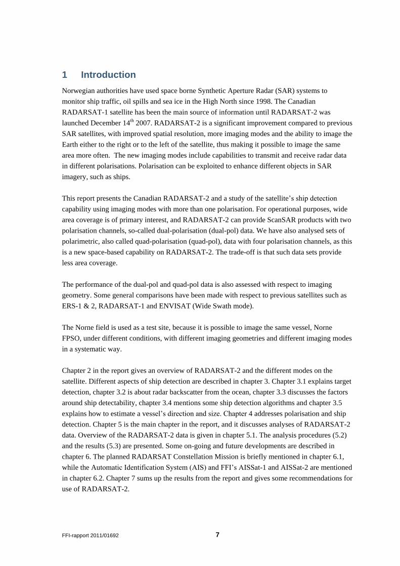
Figure 2.1 Left: Launch of RADARSAT-2 using a Soyuz rocket (© CSA).
Right: RADARSAT-2 has an inclination (i) of 98.6° (© asc-csa.gc.ca).
The satellite has a Synthetic Aperture Radar that operates in C-band (5.405 GHz), providing data
continuity from RADARSAT-1. The SAR instrument is very flexible, and can acquire data in
several modes, described in Section 2.1. Compared to Radarsat-1, spatial resolution (size of the
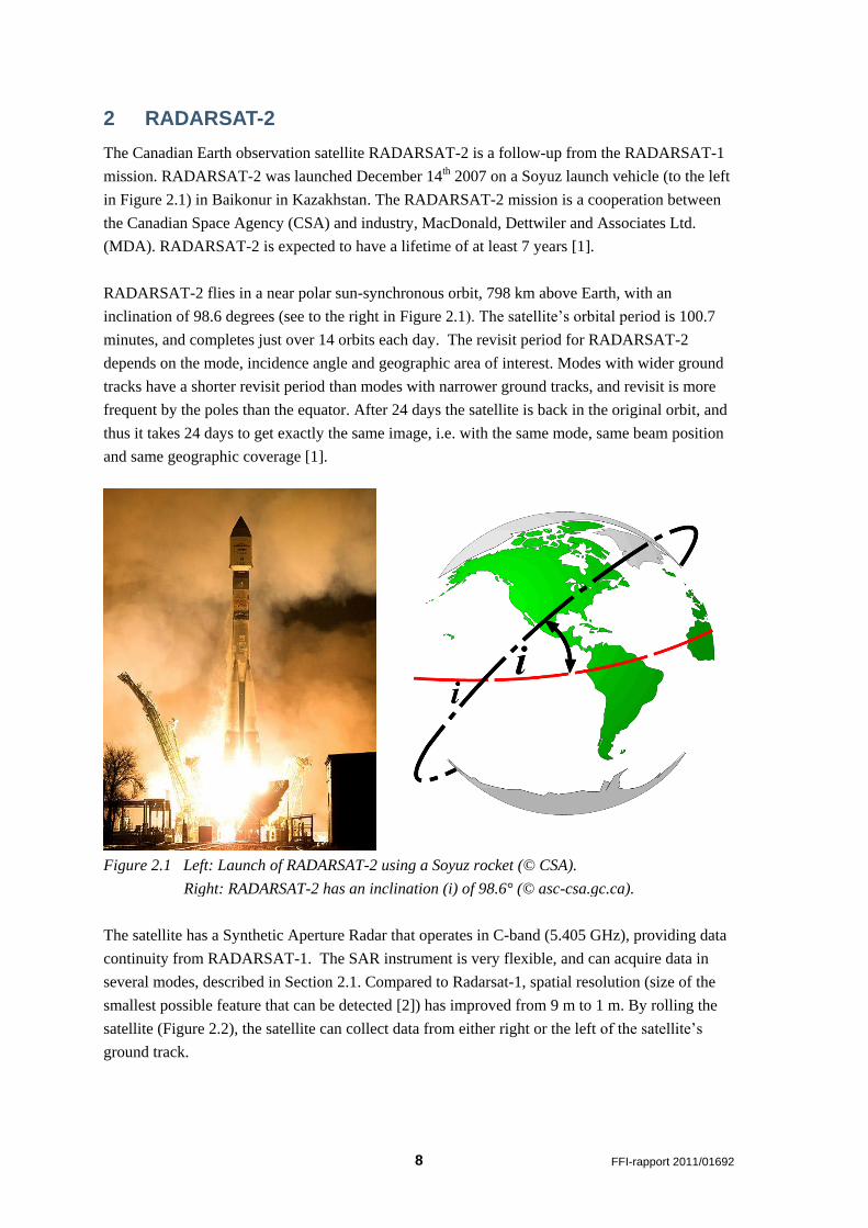
smallest possible feature that can be detected [2]) has improved from 9 m to 1 m. By rolling the
satellite (Figure 2.2), the satellite can collect data from either right or the left of the satellite’s
ground track.
FFI-rapport 2011/01692 9
Figure 2.2 The RADARSAT-2 satellite can look either to the right or to the left
(© radarsat2.info).
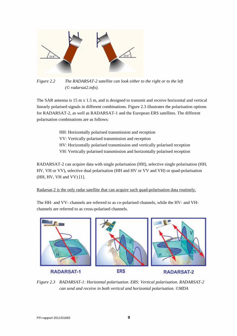
The SAR antenna is 15 m x 1.5 m, and is designed to transmit and receive horizontal and vertical
linearly polarised signals in different combinations. Figure 2.3 illustrates the polarisation options
for RADARSAT-2, as well as RADARSAT-1 and the European ERS satellites. The different
polarisation combinations are as follows:
HH: Horizontally polarised transmission and reception
VV: Vertically polarised transmission and reception
HV: Horizontally polarised transmission and vertically polarised reception
VH: Vertically polarised transmission and horizontally polarised reception
RADARSAT-2 can acquire data with single polarisation (HH), selective single polarisation (HH,
HV, VH or VV), selective dual polarisation (HH and HV or VV and VH) or quad-polarisation
(HH, HV, VH and VV) [1].
Radarsat-2 is the only radar satellite that can acquire such quad-polarisation data routinely.
The HH- and VV- channels are referred to as co-polarised channels, while the HV- and VH-
channels are referred to as cross-polarised channels.
Figure 2.3 RADARSAT-1: Horizontal polarisation. ERS: Vertical polarisation. RADARSAT-2
can send and receive in both vertical and horizontal polarisation. ©MDA
10 FFI-rapport 2011/01692
2.1 RADARSAT-2 modes
RADARSAT-1 could image in the following beam modes: Fine, Standard, Wide, ScanSAR
Narrow, ScanSAR Wide, Extended Low and Extended High. These are now referred to as the
heritage beam modes. In addition, RADARSAT-2 has Ultra-Fine, Multi-Look Fine, Fine Quad-
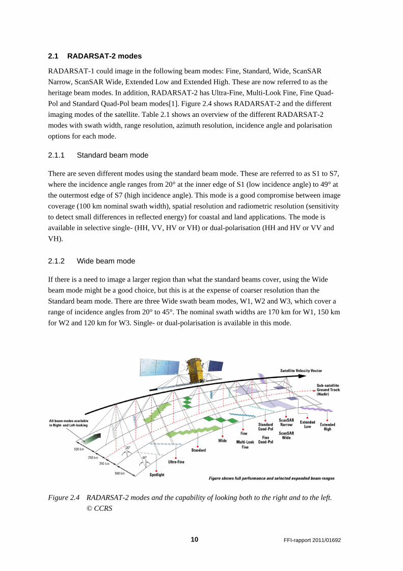
Pol and Standard Quad-Pol beam modes[1]. Figure 2.4 shows RADARSAT-2 and the different
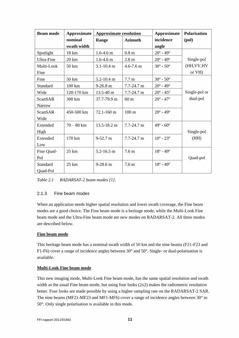
imaging modes of the satellite. Table 2.1 shows an overview of the different RADARSAT-2
modes with swath width, range resolution, azimuth resolution, incidence angle and polarisation
options for each mode.
2.1.1 Standard beam mode
There are seven different modes using the standard beam mode. These are referred to as S1 to S7,
where the incidence angle ranges from 20° at the inner edge of S1 (low incidence angle) to 49° at
the outermost edge of S7 (high incidence angle). This mode is a good compromise between image
coverage (100 km nominal swath width), spatial resolution and radiometric resolution (sensitivity
to detect small differences in reflected energy) for coastal and land applications. The mode is
available in selective single- (HH, VV, HV or VH) or dual-polarisation (HH and HV or VV and
VH).
2.1.2 Wide beam mode
If there is a need to image a larger region than what the standard beams cover, using the Wide
beam mode might be a good choice, but this is at the expense of coarser resolution than the
Standard beam mode. There are three Wide swath beam modes, W1, W2 and W3, which cover a
range of incidence angles from 20° to 45°. The nominal swath widths are 170 km for W1, 150 km
for W2 and 120 km for W3. Single- or dual-polarisation is available in this mode.
Figure 2.4 RADARSAT-2 modes and the capability of looking both to the right and to the left.
© CCRS
FFI-rapport 2011/01692 11
Beam mode Approximate
nominal
swath width
Approximate resolution Approximate
incidence
angle
Polarisation
(pol) Range Azimuth
Spotlight 18 km 1.6-4.6 m 0.8 m 20º - 49º
Single-pol
(HH,VV,HV
or VH)
Ultra-Fine 20 km 1.6-4.6 m 2.8 m 20º - 49º
Multi-Look
Fine
50 km 3.1-10.4 m 4.6-7.6 m 30º - 50º
Fine 50 km 5.2-10.4 m 7.7 m 30º - 50º
Single-pol or
dual-pol
Standard 100 km 9-26.8 m 7.7-24.7 m 20º - 49º
Wide 120-170 km 13.5-40 m 7.7-24.7 m 20º - 45º
ScanSAR
Narrow
300 km 37.7-79.9 m 60 m 20º - 47º
ScanSAR
Wide
450-500 km 72.1-160 m 100 m 20º - 49º
Extended
High
70 – 80 km 13.5-18.2 m 7.7-24.7 m 49º - 60º
Single-pol
(HH) Extended
Low
170 km 9-52.7 m 7.7-24.7 m 10º - 23º
Fine Quad-
Pol
25 km 5.2-16.5 m
7.6 m 18º - 49º
Quad-pol
Standard
Quad-Pol
25 km 9-28.6 m 7.6 m 18º - 49º
Table 2.1 RADARSAT-2 beam modes [1].
2.1.3 Fine beam modes
When an application needs higher spatial resolution and lower swath coverage, the Fine beam
modes are a good choice. The Fine beam mode is a heritage mode, while the Multi-Look Fine
beam mode and the Ultra-Fine beam mode are new modes on RADARSAT-2. All three modes
are described below.
Fine beam mode
This heritage beam mode has a nominal swath width of 50 km and the nine beams (F21-F23 and
F1-F6) cover a range of incidence angles between 30° and 50°. Single- or dual-polarisation is
available.
Multi-Look Fine beam mode
This new imaging mode, Multi-Look Fine beam mode, has the same spatial resolution and swath
width as the usual Fine beam mode, but using four looks (2x2) makes the radiometric resolution
better. Four looks are made possible by using a higher sampling rate on the RADARSAT-2 SAR.
The nine beams (MF21-MF23 and MF1-MF6) cover a range of incidence angles between 30° to
50°. Only single polarisation is available in this mode.
12 FFI-rapport 2011/01692
Ultra-Fine beam mode
When the user requires very high spatial resolution, the Ultra-Fine beams with approximately 3 m
resolution in range and azimuth can be used. The incidence angle ranges between 20° to 49° and
the nominal swath width is at least 20 km. The Ultra-Fine beam imaging mode offers only single
polarisation.
2.1.4 Extended beam mode
Some minor degradation of the image can happen because the antenna operates beyond the
optimum range for the Extended beams. Only single polarisation (HH) is available.
Extended Low beam mode
The Extended Low beam mode has a single beam (EL1) with a swath width of 170 km and an
incidence angle range from 10° to 23°.
Extended High beam mode
The Extended High beam mode covers the incidence angles from 49° to 60°. The inner three
beams (EH1-EH3) have swath width of 80 km, while the swath width is 70 km for the three outer
beams (EH4-EH6).
2.1.5 Quad-Pol modes
If quad-polarised data are required, the Fine or Standard Quad-Pol modes can be used. Then the
user gets four images in HH-, VV-, HV- and VH-polarisation. The Quad-Pol modes have a
nominal swath width of 25 km. The many beams in the Standard and Fine Quad-Pol modes cover
a range of incidence angles from 18° to 49°.
2.1.6 ScanSAR mode
ScanSAR images have been used operationally by the Norwegian Defence to monitor Norway’s
large ocean areas. It is possible to get images in single- or dual-polarisation using the ScanSAR
modes.
ScanSAR Narrow (SCN)
The ScanSAR Narrow mode has two different combinations. SCNA is a combination of W1 and
W2, while SCNB is a combination of W2, S5 and S6. The incidence angle ranges from 20° to 39°
for SCNA and from 31° to 47° for SCNB. The swath width is about 300 km.
ScanSAR Wide (SCW)
ScanSAR Wide images have the largest swath coverage on RADARSAT-2. This is obtained by
combining single beams adjoining each other. The increased coverage is good to use to get an
overview of the ocean, but the cost is lower resolution. Two combinations can be used. SCWA
has a swath width of more than 500 km and is a combination of W1, W2, W3 and S7. SCWB has
FFI-rapport 2011/01692 13
a swath width of more than 450 km and is a combination of W1, W2, S5 and S6. The incidence
angle ranges from 20° to 49° for SCWA and from 20° to 46° for SCWB.
2.1.7 Spotlight beam mode
The Spotlight beams are for users who require high resolution. The Spotlight beam mode offers
the highest available resolution (1 m) on RADARSAT-2. The swath width of each beam is at
least 18 km. The beams cover a range of incidence angles from 20° to 49°.
3 Ship detection
Two ways to detect ships are to use target detection and detection of ship wakes. Target detection
is regarded as the most effective method within automatic ship detection. If one believes a ship is
detected, ship wake detection can be pursued to confirm if it really is a ship. Fisheries monitoring
is one of the main applications of SAR ship detection. When fishing, the vessels are usually
moving too slowly to make significant ship wakes. We have therefore focused on target detection
in the following sections.
3.1 Target detection
To detect ships one must be able to recognize bright point targets in an ocean clutter background.
The contrast can be measured as the maximum value of the ship compared to the average
background signal from the ocean. The contrast can also be measured as the Target to Clutter
Ratio (TCR), which can be defined as the ratio of a ship’s normalized radar cross section and the
average radar reflection (ocean clutter) from the surrounding background. If the ocean
background reflection is weak, the background signal can be dominated by thermal noise from the
radar instrument. The TCR will then give the ratio of the measured signal of the ship compared to
the background noise in the measurement.
In order to maximize the TCR, we can select radar parameters that either maximize the radar
returns of ships, or suppress ocean clutter, or preferably do both. Radar returns from ships depend
on their size, orientation compared to the radar look direction and superstructure. Other factors
are radar polarisation, incidence angle and ships’ motion. Little information has been published
on the relationship between radar polarisation and ship reflections. In the following sections, we
assume that cross-pol reflections for ships are ~10 dB lower than for corresponding co-pol
measurements.
14 FFI-rapport 2011/01692
The new availability of polarimetric data from RADARSAT-2 will provide opportunities to
examine this in more detail. A weak dependency on incidence angle (θ) for the radar reflection
has been reported in [3]:
11.078.0)( R (3.1)
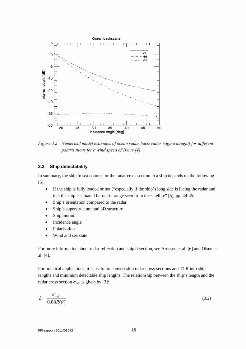
3.2 Ocean Clutter
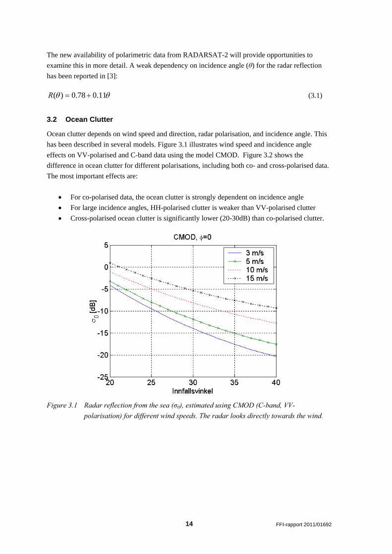
Ocean clutter depends on wind speed and direction, radar polarisation, and incidence angle. This
has been described in several models. Figure 3.1 illustrates wind speed and incidence angle
effects on VV-polarised and C-band data using the model CMOD. Figure 3.2 shows the
difference in ocean clutter for different polarisations, including both co- and cross-polarised data.
The most important effects are:
For co-polarised data, the ocean clutter is strongly dependent on incidence angle
For large incidence angles, HH-polarised clutter is weaker than VV-polarised clutter
Cross-polarised ocean clutter is significantly lower (20-30dB) than co-polarised clutter.
Figure 3.1 Radar reflection from the sea (σ0), estimated using CMOD (C-band, VV-
polarisation) for different wind speeds. The radar looks directly towards the wind.
FFI-rapport 2011/01692 15
Figure 3.2 Numerical model estimates of ocean radar backscatter (sigma nought) for different
polarisations for a wind speed of 10m/s [4].
3.3 Ship detectability
In summary, the ship to sea contrast or the radar cross section to a ship depends on the following
[5]:
If the ship is fully loaded or not (“especially if the ship’s long side is facing the radar and
that the ship is situated far out in range seen from the satellite” [5], pp. 44-45.
Ship’s orientation compared to the radar
Ship’s superstructure and 3D structure
Ship motion
Incidence angle
Polarisation
Wind and sea state
For more information about radar reflection and ship detection, see Arnesen et al. [6] and Olsen et
al. [4].
For practical applications, it is useful to convert ship radar cross-sections and TCR into ship
lengths and minimum detectable ship lengths. The relationship between the ship’s length and the
radar cross section σship is given by [3]:
)(08.0
RL ship (3.2)

16 FFI-rapport 2011/01692
To be able to estimate the radar cross section for the smallest ship that is possible to detect, one
can use a threshold value, T, for the average backscattering or the noise floor:
10/)(min 10 T
arshipsea (3.3)
ρr and ρa are the SAR resolution in range and azimuth direction, respectively and σsea is the ocean
backscatter. A threshold value, T, 10 dB above σsea is useful for images with low and moderate
resolution.
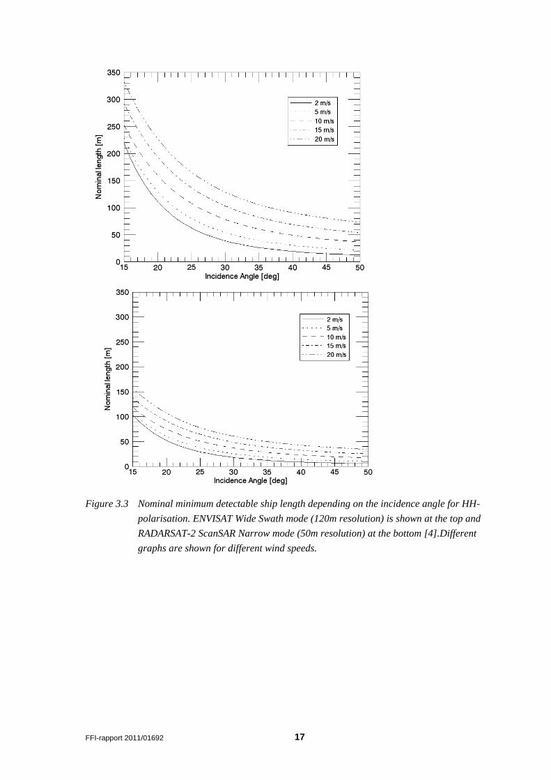
We can use the expressions above to calculate theoretical minimum detectable ship sizes for
different combinations of incidence angles and, wind speeds, radar resolutions and polarisations,
as shown in Figure 3.3 and Figure 3.4. Figure 3.3 shows a comparison between ENVISAT Wide
Swath mode (120 m resolution) and RADARSAT-2 ScanSAR Narrow mode (50 m resolution)for
HH-polarisation. The plot for RADARSAT-2 (bottom half) is valid for both RADARSAT-1 and
RADARSAT-2. RADARSAT performance is better than for ENVISAT, due to the better spatial
resolution of the ScanSAR Narrow mode compared to the Wide Swath mode of ENVISAT.
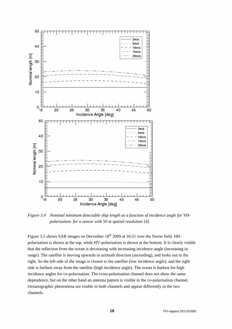
Figure 3.4 shows similar curves for VH-polarised data. We see that ships of the order of 20-30 m
in length should be detectable even in strong winds. The upper panel is valid for RADARSAT-2
ScanSAR Narrow mode (50 m resolution). The lower panel shows what could be achieved with a
lower noise floor, and is representative for RADARSAT-2 Standard Quad-Pol mode. It is
assumed a 10dB reduction in ship signature from co-pol to cross-pol data, and a noise floor of -
28dB and-36dB.
Extensive research on ENVISAT Alternating Polarisation (AP) data has been done in [6]. The
polarisation combinations VV/VH, HH/HV and VV/HH have been explored. The research
indicated that cross-polarised radar should be best for small incidence angles (15-30), while co-
polarised radar should be best for larger incidence angles.
FFI-rapport 2011/01692 17
Figure 3.3 Nominal minimum detectable ship length depending on the incidence angle for HH-
polarisation. ENVISAT Wide Swath mode (120m resolution) is shown at the top and
RADARSAT-2 ScanSAR Narrow mode (50m resolution) at the bottom [4].Different
graphs are shown for different wind speeds.
18 FFI-rapport 2011/01692
Figure 3.4 Nominal minimum detectable ship length as a function of incidence angle for VH-
polarisation. for a sensor with 50 m spatial resolution [4].
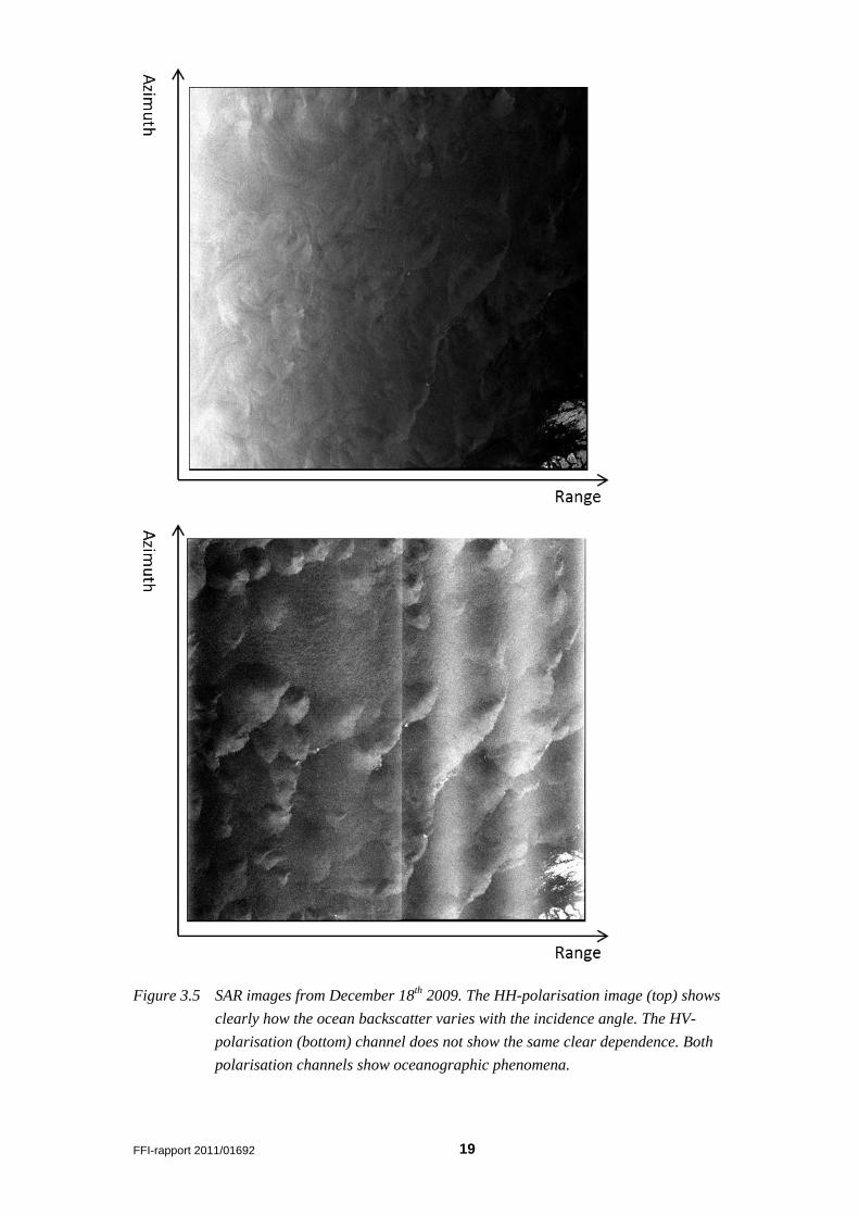
Figure 3.5 shows SAR images on December 18th 2009 at 16:51 over the Norne field. HH-
polarisation is shown at the top, while HV-polarisation is shown at the bottom. It is clearly visible
that the reflection from the ocean is decreasing with increasing incidence angle (increasing in
range). The satellite is moving upwards in azimuth direction (ascending), and looks out to the
right. So the left side of the image is closest to the satellite (low incidence angle), and the right
side is farthest away from the satellite (high incidence angle). The ocean is darkest for high
incidence angles for co-polarisation. The cross-polarisation channel does not show the same
dependence, but on the other hand an antenna pattern is visible in the co-polarisation channel.
Oceanographic phenomena are visible in both channels and appear differently in the two
channels.
FFI-rapport 2011/01692 19
Figure 3.5 SAR images from December 18th 2009. The HH-polarisation image (top) shows
clearly how the ocean backscatter varies with the incidence angle. The HV-
polarisation (bottom) channel does not show the same clear dependence. Both
polarisation channels show oceanographic phenomena.
20 FFI-rapport 2011/01692
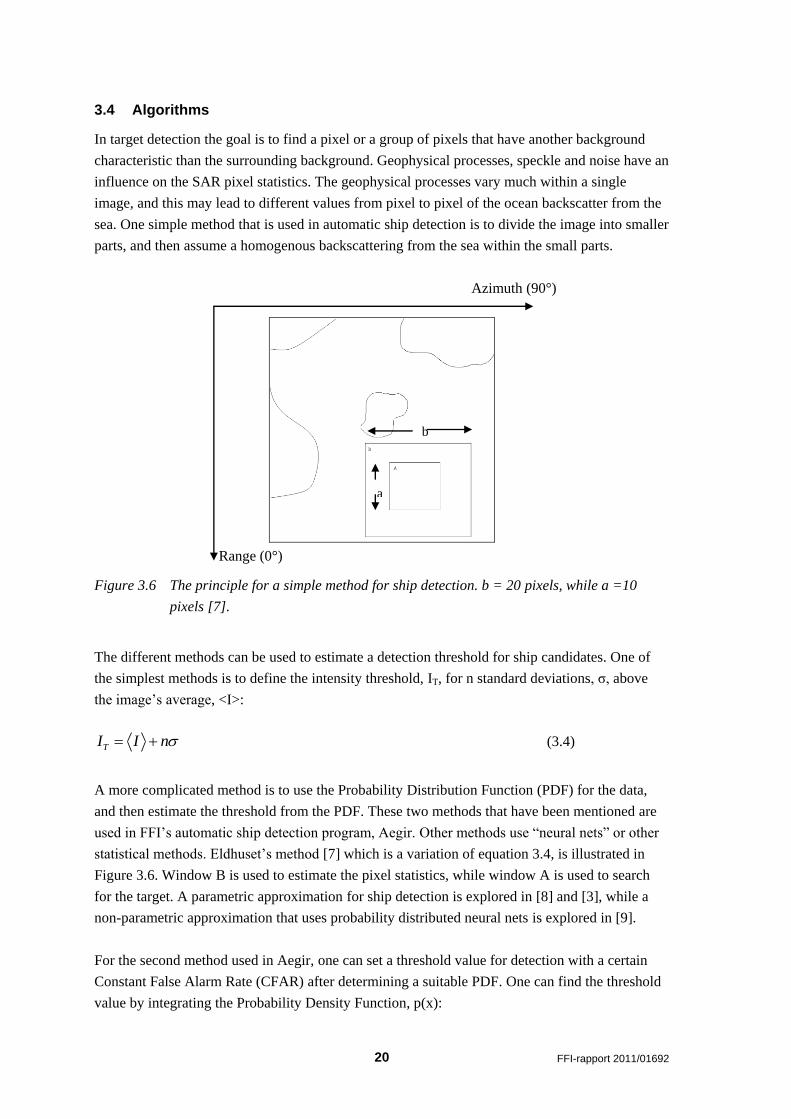
3.4 Algorithms
In target detection the goal is to find a pixel or a group of pixels that have another background
characteristic than the surrounding background. Geophysical processes, speckle and noise have an
influence on the SAR pixel statistics. The geophysical processes vary much within a single
image, and this may lead to different values from pixel to pixel of the ocean backscatter from the
sea. One simple method that is used in automatic ship detection is to divide the image into smaller
parts, and then assume a homogenous backscattering from the sea within the small parts.
Azimuth (90°)
Range (0°)
Figure 3.6 The principle for a simple method for ship detection. b = 20 pixels, while a =10
pixels [7].
The different methods can be used to estimate a detection threshold for ship candidates. One of
the simplest methods is to define the intensity threshold, IT, for n standard deviations, σ, above
the image’s average, <I>:
TI I n (3.4)
A more complicated method is to use the Probability Distribution Function (PDF) for the data,
and then estimate the threshold from the PDF. These two methods that have been mentioned are
used in FFI’s automatic ship detection program, Aegir. Other methods use “neural nets” or other
statistical methods. Eldhuset’s method [7] which is a variation of equation 3.4, is illustrated in
Figure 3.6. Window B is used to estimate the pixel statistics, while window A is used to search
for the target. A parametric approximation for ship detection is explored in [8] and [3], while a
non-parametric approximation that uses probability distributed neural nets is explored in [9].
For the second method used in Aegir, one can set a threshold value for detection with a certain
Constant False Alarm Rate (CFAR) after determining a suitable PDF. One can find the threshold
value by integrating the Probability Density Function, p(x):
b
a
FFI-rapport 2011/01692 21
TI
dxxpCFAR0
)( (3.5)
where CFAR is the user-specified false alarm rate, for example 10-7. By using this value in a
characteristic SAR image, there will be some pixels that will be characterized as a ship by
mistake. So when using the method described above, one must find a balance between detection
rate and occurrence of false alarms. False alarms can be reduced by taking some precautions and
by using homogeneity tests [7], morphological filters, analyses of ship wakes [7;8;10] or a
combination of these methods.
3.5 Vessel’s direction and size
A vessel’s direction can be estimated both by analysing the point target and by analysing the ship
wake signature (if detectable). Problems can arise when the target is rotating and if there is
smearing of the target, for example if a vessel is moving. The ship wake signature probably gives
the best estimation. Where the ship wake signature is not detectable, an analysis of the point
target can give some information about the vessel’s moving direction. To be able to estimate the
vessel’s size, several methods exist, for example geometrical methods based on the number of
pixels that are part of the vessel as well as using the radar cross section. These methods are not
described in this report.
4 Polarisation and ship detection
Polarisation is an important factor when working with ship detection. Different materials and
surfaces have different scattering properties in the different polarisations and polarisation
combinations. The structure of the ship, the ship’s orientation compared to the radar, motion and
sea state all play an important role on how a vessel reflects the radar signals back to the satellite.
Depending on how complex the ship’s superstructure is, the number of reflections from the
surface of the ship can be both even (double) and odd (single and triple) and in addition
reflections can occur from corners, edges and cables on the ship [4].
Research in polarimetry has resulted in a number of ways to combine the different polarisation
channels, as well as various interpretations of the scattering mechanisms associated with the
individual and combined polarisation options.
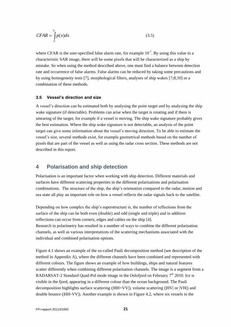
Figure 4.1 shows an example of the so-called Pauli decomposition method (see description of the
method in Appendix A), where the different channels have been combined and represented with
different colours. The figure shows an example of how buildings, ships and natural features
scatter differently when combining different polarisation channels. The image is a segment from a
RADARSAT-2 Standard Quad-Pol mode image in the Oslofjord on February 7th 2010. Ice is
visible in the fjord, appearing in a different colour than the ocean background. The Pauli
decomposition highlights surface scattering (|HH+VV|), volume scattering (|HV| or |VH|) and
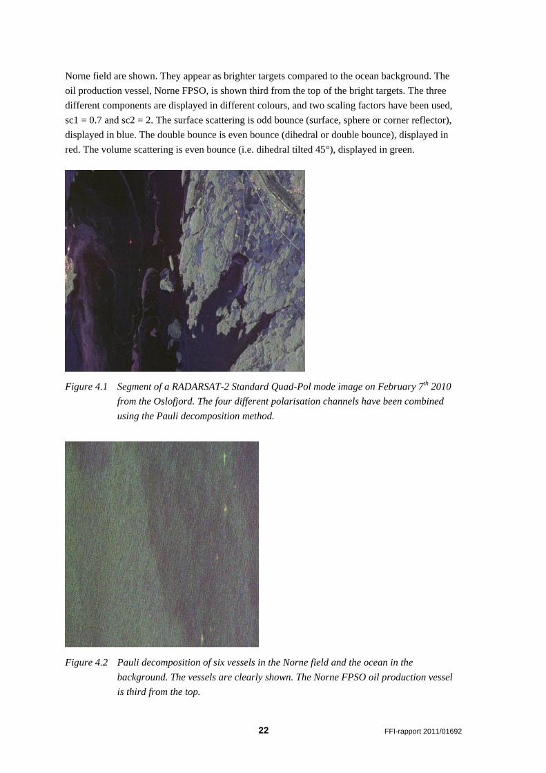
double bounce (|HH-VV|). Another example is shown in Figure 4.2, where six vessels in the
22 FFI-rapport 2011/01692
Norne field are shown. They appear as brighter targets compared to the ocean background. The
oil production vessel, Norne FPSO, is shown third from the top of the bright targets. The three
different components are displayed in different colours, and two scaling factors have been used,
sc1 = 0.7 and sc2 = 2. The surface scattering is odd bounce (surface, sphere or corner reflector),
displayed in blue. The double bounce is even bounce (dihedral or double bounce), displayed in
red. The volume scattering is even bounce (i.e. dihedral tilted 45°), displayed in green.
Figure 4.1 Segment of a RADARSAT-2 Standard Quad-Pol mode image on February 7th 2010
from the Oslofjord. The four different polarisation channels have been combined
using the Pauli decomposition method.
Figure 4.2 Pauli decomposition of six vessels in the Norne field and the ocean in the
background. The vessels are clearly shown. The Norne FPSO oil production vessel
is third from the top.
FFI-rapport 2011/01692 23
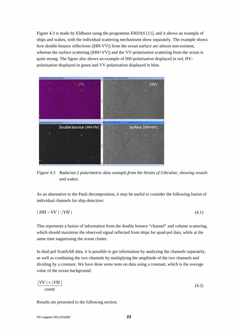
Figure 4.3 is made by Eldhuset using the programme ERDAS [11], and it shows an example of
ships and wakes, with the individual scattering mechanisms show separately. The example shows
how double bounce reflections (|HH-VV|) from the ocean surface are almost non-existent,
whereas the surface scattering (|HH+VV|) and the VV-polarisation scattering from the ocean is
quite strong. The figure also shows an example of HH-polarisation displayed in red, HV-
polarisation displayed in green and VV-polarisation displayed in blue.
Figure 4.3 Radarsat-2 polarimetric data example,from the Straits of Gibraltar, showing vessels
and wakes.
As an alternative to the Pauli decomposition, it may be useful to consider the following fusion of
individual channels for ship detection:
|||| VHVVHH (4.1)
This represents a fusion of information from the double bounce “channel” and volume scattering,
which should maximise the observed signal reflected from ships for quad-pol data, while at the
same time suppressing the ocean clutter.
In dual-pol ScanSAR data, it is possible to get information by analysing the channels separately,
as well as combining the two channels by multiplying the amplitude of the two channels and
dividing by a constant. We have done some tests on data using a constant, which is the average
value of the ocean background.
const
VHVV |||| (4.2)
Results are presented in the following section.
24 FFI-rapport 2011/01692
5 Analysis of RADARSAT-2 data
This section presents an evaluation of some of the modes and polarisation options that
RADARSAT-2 offers. The test field used is the Norne field, west of central Norway.
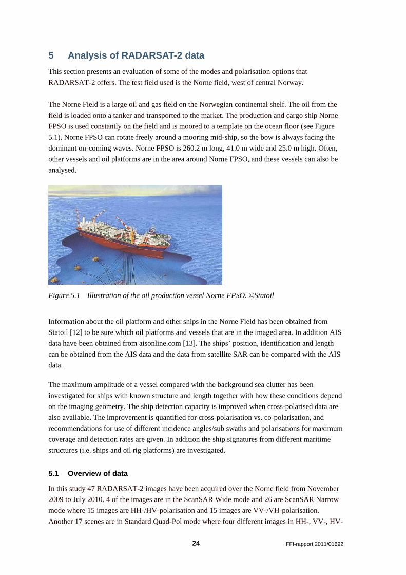
The Norne Field is a large oil and gas field on the Norwegian continental shelf. The oil from the
field is loaded onto a tanker and transported to the market. The production and cargo ship Norne
FPSO is used constantly on the field and is moored to a template on the ocean floor (see Figure
5.1). Norne FPSO can rotate freely around a mooring mid-ship, so the bow is always facing the
dominant on-coming waves. Norne FPSO is 260.2 m long, 41.0 m wide and 25.0 m high. Often,
other vessels and oil platforms are in the area around Norne FPSO, and these vessels can also be
analysed.
Figure 5.1 Illustration of the oil production vessel Norne FPSO. ©Statoil
Information about the oil platform and other ships in the Norne Field has been obtained from
Statoil [12] to be sure which oil platforms and vessels that are in the imaged area. In addition AIS
data have been obtained from aisonline.com [13]. The ships’ position, identification and length
can be obtained from the AIS data and the data from satellite SAR can be compared with the AIS
data.
The maximum amplitude of a vessel compared with the background sea clutter has been
investigated for ships with known structure and length together with how these conditions depend
on the imaging geometry. The ship detection capacity is improved when cross-polarised data are
also available. The improvement is quantified for cross-polarisation vs. co-polarisation, and
recommendations for use of different incidence angles/sub swaths and polarisations for maximum
coverage and detection rates are given. In addition the ship signatures from different maritime
structures (i.e. ships and oil rig platforms) are investigated.
5.1 Overview of data
In this study 47 RADARSAT-2 images have been acquired over the Norne field from November
2009 to July 2010. 4 of the images are in the ScanSAR Wide mode and 26 are ScanSAR Narrow
mode where 15 images are HH-/HV-polarisation and 15 images are VV-/VH-polarisation.
Another 17 scenes are in Standard Quad-Pol mode where four different images in HH-, VV-, HV-
FFI-rapport 2011/01692 25
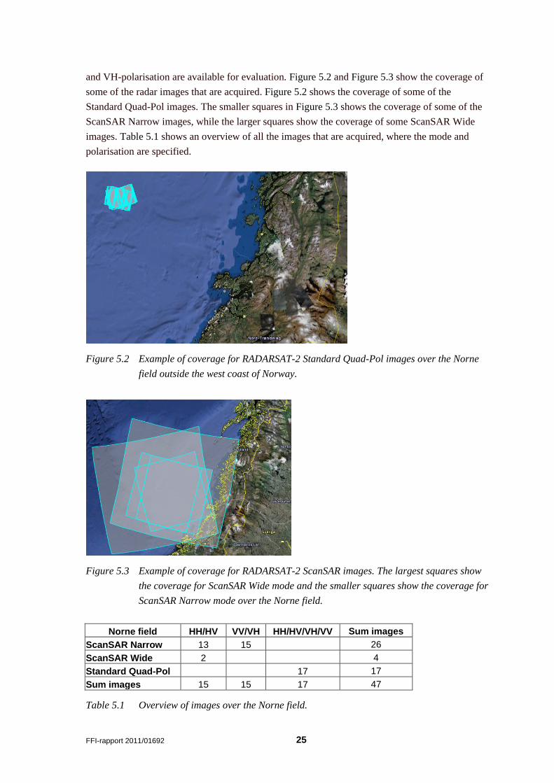
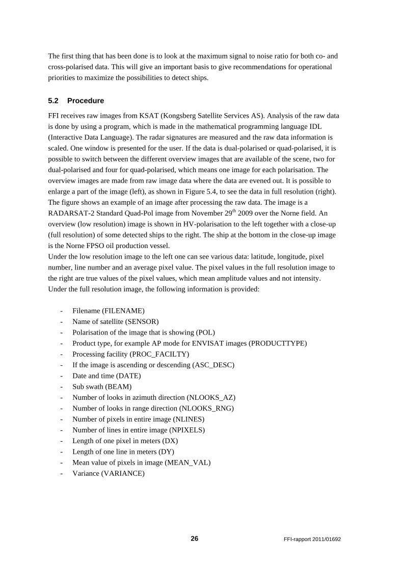
and VH-polarisation are available for evaluation. Figure 5.2 and Figure 5.3 show the coverage of
some of the radar images that are acquired. Figure 5.2 shows the coverage of some of the
Standard Quad-Pol images. The smaller squares in Figure 5.3 shows the coverage of some of the
ScanSAR Narrow images, while the larger squares show the coverage of some ScanSAR Wide
images. Table 5.1 shows an overview of all the images that are acquired, where the mode and
polarisation are specified.
Figure 5.2 Example of coverage for RADARSAT-2 Standard Quad-Pol images over the Norne
field outside the west coast of Norway.
Figure 5.3 Example of coverage for RADARSAT-2 ScanSAR images. The largest squares show
the coverage for ScanSAR Wide mode and the smaller squares show the coverage for
ScanSAR Narrow mode over the Norne field.
Norne field HH/HV VV/VH HH/HV/VH/VV Sum images
ScanSAR Narrow 13 15 26
ScanSAR Wide 2 4
Standard Quad-Pol 17 17
Sum images 15 15 17 47
Table 5.1 Overview of images over the Norne field.
26 FFI-rapport 2011/01692
The first thing that has been done is to look at the maximum signal to noise ratio for both co- and
cross-polarised data. This will give an important basis to give recommendations for operational
priorities to maximize the possibilities to detect ships.
5.2 Procedure
FFI receives raw images from KSAT (Kongsberg Satellite Services AS). Analysis of the raw data
is done by using a program, which is made in the mathematical programming language IDL
(Interactive Data Language). The radar signatures are measured and the raw data information is
scaled. One window is presented for the user. If the data is dual-polarised or quad-polarised, it is
possible to switch between the different overview images that are available of the scene, two for
dual-polarised and four for quad-polarised, which means one image for each polarisation. The
overview images are made from raw image data where the data are evened out. It is possible to
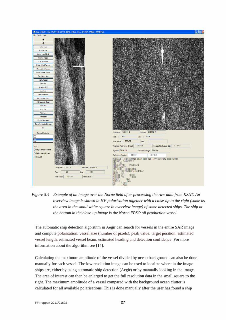
enlarge a part of the image (left), as shown in Figure 5.4, to see the data in full resolution (right).
The figure shows an example of an image after processing the raw data. The image is a
RADARSAT-2 Standard Quad-Pol image from November 29th 2009 over the Norne field. An
overview (low resolution) image is shown in HV-polarisation to the left together with a close-up
(full resolution) of some detected ships to the right. The ship at the bottom in the close-up image
is the Norne FPSO oil production vessel.
Under the low resolution image to the left one can see various data: latitude, longitude, pixel
number, line number and an average pixel value. The pixel values in the full resolution image to
the right are true values of the pixel values, which mean amplitude values and not intensity.
Under the full resolution image, the following information is provided:
- Filename (FILENAME)
- Name of satellite (SENSOR)
- Polarisation of the image that is showing (POL)
- Product type, for example AP mode for ENVISAT images (PRODUCTTYPE)
- Processing facility (PROC_FACILTY)
- If the image is ascending or descending (ASC_DESC)
- Date and time (DATE)
- Sub swath (BEAM)
- Number of looks in azimuth direction (NLOOKS_AZ)
- Number of looks in range direction (NLOOKS_RNG)
- Number of pixels in entire image (NLINES)
- Number of lines in entire image (NPIXELS)
- Length of one pixel in meters (DX)
- Length of one line in meters (DY)
- Mean value of pixels in image (MEAN_VAL)
- Variance (VARIANCE)
FFI-rapport 2011/01692 27
Figure 5.4 Example of an image over the Norne field after processing the raw data from KSAT. An
overview image is shown in HV-polarisation together with a close-up to the right (same as
the area in the small white square in overview image) of some detected ships. The ship at
the bottom in the close-up image is the Norne FPSO oil production vessel.
The automatic ship detection algorithm in Aegir can search for vessels in the entire SAR image
and compute polarisation, vessel size (number of pixels), peak value, target position, estimated
vessel length, estimated vessel beam, estimated heading and detection confidence. For more
information about the algorithm see [14].
Calculating the maximum amplitude of the vessel divided by ocean background can also be done
manually for each vessel. The low resolution image can be used to localize where in the image
ships are, either by using automatic ship detection (Aegir) or by manually looking in the image.
The area of interest can then be enlarged to get the full resolution data in the small square to the
right. The maximum amplitude of a vessel compared with the background ocean clutter is
calculated for all available polarisations. This is done manually after the user has found a ship
28 FFI-rapport 2011/01692
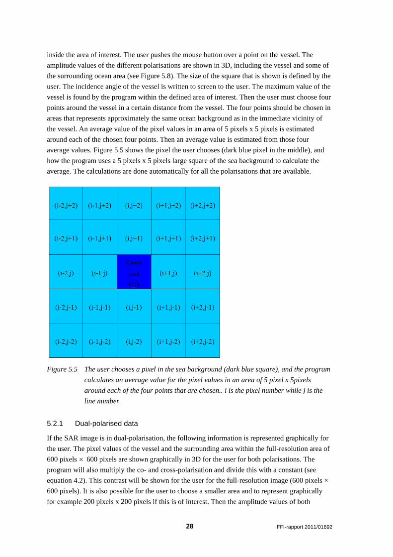
inside the area of interest. The user pushes the mouse button over a point on the vessel. The
amplitude values of the different polarisations are shown in 3D, including the vessel and some of
the surrounding ocean area (see Figure 5.8). The size of the square that is shown is defined by the
user. The incidence angle of the vessel is written to screen to the user. The maximum value of the
vessel is found by the program within the defined area of interest. Then the user must choose four
points around the vessel in a certain distance from the vessel. The four points should be chosen in
areas that represents approximately the same ocean background as in the immediate vicinity of
the vessel. An average value of the pixel values in an area of 5 pixels x 5 pixels is estimated
around each of the chosen four points. Then an average value is estimated from those four
average values. Figure 5.5 shows the pixel the user chooses (dark blue pixel in the middle), and
how the program uses a 5 pixels x 5 pixels large square of the sea background to calculate the
average. The calculations are done automatically for all the polarisations that are available.
Figure 5.5 The user chooses a pixel in the sea background (dark blue square), and the program
calculates an average value for the pixel values in an area of 5 pixel x 5pixels
around each of the four points that are chosen.. i is the pixel number while j is the
line number.
5.2.1 Dual-polarised data
If the SAR image is in dual-polarisation, the following information is represented graphically for
the user. The pixel values of the vessel and the surrounding area within the full-resolution area of
600 pixels 600 pixels are shown graphically in 3D for the user for both polarisations. The
program will also multiply the co- and cross-polarisation and divide this with a constant (see
equation 4.2). This contrast will be shown for the user for the full-resolution image (600 pixels ×
600 pixels). It is also possible for the user to choose a smaller area and to represent graphically
for example 200 pixels x 200 pixels if this is of interest. Then the amplitude values of both
FFI-rapport 2011/01692 29
channels are shown graphically in two separate windows, as well as the combined case (co- and
cross-polarised channels multiplied and divided by a constant).
In the end a contrast analysis is done, and the results of the contrast measures are written to file.
The maximum amplitude, the mean sea and the ratio between these values are estimated and
given for both polarisations and also for the combined case as estimated using equation 4.2.
5.2.2 Quad-polarised data
If the SAR image is in quad-polarisation, the following information is represented graphically for
the user. The pixel values of the vessel and the surrounding area within the full-resolution area of
600 pixels x 600 pixels are shown graphically in 3D for the user for all four polarisations. The
program will also use circular basis decomposition (see Appendix B) to find the amplitude values
for SRL (Right-Left), SLR (Left-Right), SRR (Right-Right) and SLL (Left-Left) elements, in addition
to |HH-VV| (double bounce) and |HH-VV|*|HV| (double bounce multiplied by volume
scattering).
The program will also do Pauli decomposition on the image, and the user can choose to do it on
the entire image or only part of the image. The method is done by blocks, 1200 lines in each
block, and is saved to file. In addition Pauli method is done on the entire image. The image is also
resized to normal size due to the number of looks (1 x 4).
In the end a contrast analysis is done and the results of the contrast measures are written to file.
The maximum amplitude, the mean sea and the ratio between these values are estimated and
given for all four polarisations, as well as for SRL, SLR, SRR, SLL, |HH-VV| and |HH-VV|*|HV|.
5.3 Results
5.3.1 Dual-polarised data
Dual-polarised data may be better for operational use since the data are available in wider swaths,
i.e. the temporal coverage is better. When dual-polarised data are available, it is possible to get
information by looking at the channels separately and also by combining the two channels by
multiplying the amplitude of the two channels and dividing by a constant.
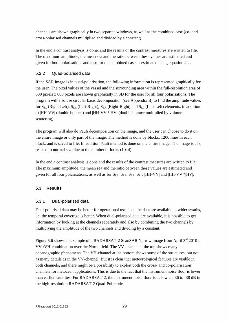
Figure 5.6 shows an example of a RADARSAT-2 ScanSAR Narrow image from April 3rd 2010 in
VV-/VH-combination over the Norne field. The VV-channel at the top shows many
oceanographic phenomena. The VH-channel at the bottom shows some of the structures, but not
as many details as in the VV-channel. But it is clear that meteorological features are visible in
both channels, and there might be a possibility to exploit both the cross- and co-polarisation
channels for metocean applications. This is due to the fact that the instrument noise floor is lower
than earlier satellites. For RADARSAT-2, the instrument noise floor is as low as -36 to -38 dB in
the high-resolution RADARSAT-2 Quad-Pol mode.
30 FFI-rapport 2011/01692
Figure 5.6 Dual-polarised data from April 3rd
2010. The VV-channel at the top shows many
oceanographic phenomena. The VH-channel shows some of the structures, but not as
many details as in the VV-channel.
FFI-rapport 2011/01692 31
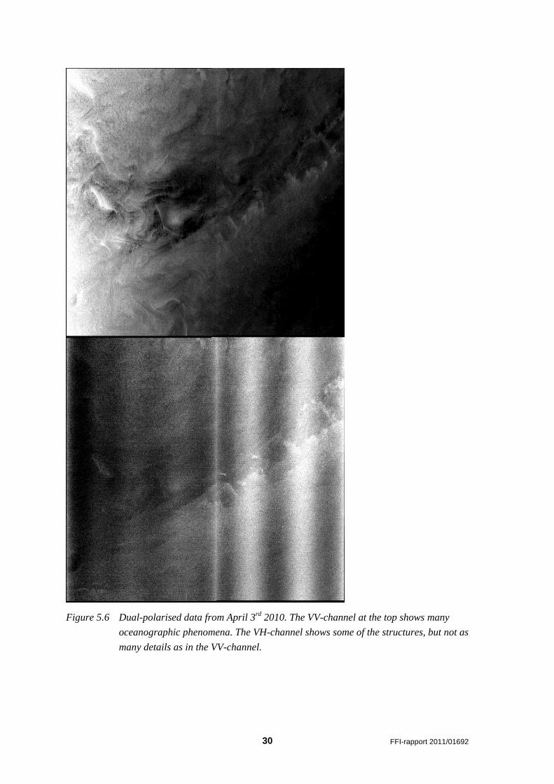
Figure 5.7 The difference between VV-polarisation (left) and VH-polarisation (right). The segments
are from a RADARSAT-2 ScanSAR Narrow image over the Norne field on April 5th 2010.
AIS data are shown at the bottom.
Figure 5.7 shows the difference between the VV- and the VH-polarisation channels. AIS-data are
shown at the bottom. The example is a segment from a RADARSAT-2 ScanSAR Narrow image
over the Norne field on April 5th 2010. The ocean seems to be darker in the co-polarisation
channel (left) than in the cross-polarisation channel (right). The vessels are visible in both
polarisation channels (except Ocean Prince). Norne FPSO and Navion Oceania are situated next
to each other, so it is hard to distinguish the two vessels both in the SAR image and in the figure
showing the ship signatures (Figure 5.8).
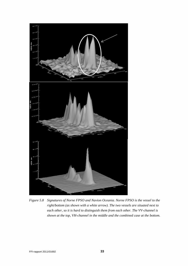
Figure 5.8 shows the signatures of Norne FPSO and Navion Oceania in the different polarisation
channels and also when combining the two channels. Norne FPSO is the vessel to the
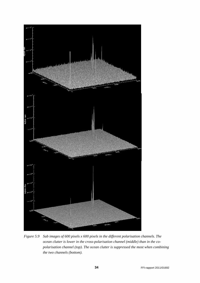
right/bottom and Navion Oceania is the vessel to the left/top. Figure 5.9 shows sub images of 600
32 FFI-rapport 2011/01692
pixels x 600 pixels of the different channels and in the combined case. The ocean clutter is lower
in the cross-polarisation channel than in the co-polarisation channel. The ocean clutter is
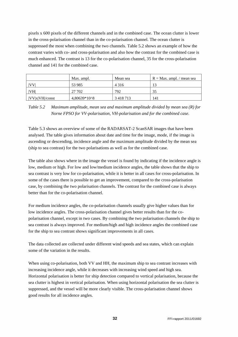
suppressed the most when combining the two channels. Table 5.2 shows an example of how the
contrast varies with co- and cross-polarisation and also how the contrast for the combined case is
much enhanced. The contrast is 13 for the co-polarisation channel, 35 for the cross-polarisation
channel and 141 for the combined case.
Max. ampl. Mean sea R = Max. ampl. / mean sea
|VV| 53 985 4 316 13
|VH| 27 702 792 35
|VV|x|VH|/const 4,80639*10^8 3 418 713 141
Table 5.2 Maximum amplitude, mean sea and maximum amplitude divided by mean sea (R) for
Norne FPSO for VV-polarisation, VH-polarisation and for the combined case.
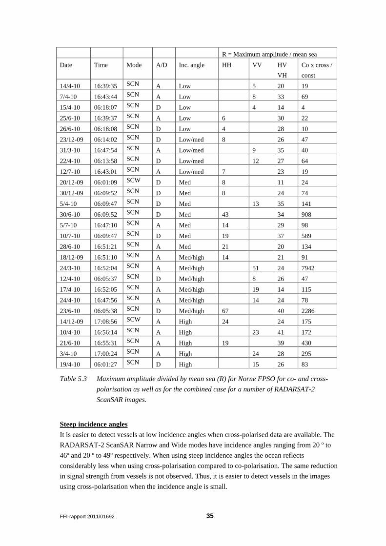
Table 5.3 shows an overview of some of the RADARSAT-2 ScanSAR images that have been
analysed. The table gives information about date and time for the image, mode, if the image is
ascending or descending, incidence angle and the maximum amplitude divided by the mean sea
(ship to sea contrast) for the two polarisations as well as for the combined case.
The table also shows where in the image the vessel is found by indicating if the incidence angle is
low, medium or high. For low and low/medium incidence angles, the table shows that the ship to
sea contrast is very low for co-polarisation, while it is better in all cases for cross-polarisation. In
some of the cases there is possible to get an improvement, compared to the cross-polarisation
case, by combining the two polarisation channels. The contrast for the combined case is always
better than for the co-polarisation channel.
For medium incidence angles, the co-polarisation channels usually give higher values than for
low incidence angles. The cross-polarisation channel gives better results than for the co-
polarisation channel, except in two cases. By combining the two polarisation channels the ship to
sea contrast is always improved. For medium/high and high incidence angles the combined case
for the ship to sea contrast shows significant improvements in all cases.
The data collected are collected under different wind speeds and sea states, which can explain
some of the variation in the results.
When using co-polarisation, both VV and HH, the maximum ship to sea contrast increases with
increasing incidence angle, while it decreases with increasing wind speed and high sea.
Horizontal polarisation is better for ship detection compared to vertical polarisation, because the
sea clutter is highest in vertical polarisation. When using horizontal polarisation the sea clutter is
suppressed, and the vessel will be more clearly visible. The cross-polarisation channel shows
good results for all incidence angles.
FFI-rapport 2011/01692 33
Figure 5.8 Signatures of Norne FPSO and Navion Oceania. Norne FPSO is the vessel to the
right/bottom (as shown with a white arrow). The two vessels are situated next to
each other, so it is hard to distinguish them from each other. The VV-channel is
shown at the top, VH-channel in the middle and the combined case at the bottom.
34 FFI-rapport 2011/01692
Figure 5.9 Sub images of 600 pixels x 600 pixels in the different polarisation channels. The
ocean clutter is lower in the cross-polarisation channel (middle) than in the co-
polarisation channel (top). The ocean clutter is suppressed the most when combining
the two channels (bottom).
FFI-rapport 2011/01692 35
R = Maximum amplitude / mean sea
Date Time Mode A/D Inc. angle HH VV HV
VH
Co x cross /
const
14/4-10 16:39:35 SCN A Low 5 20 19
7/4-10 16:43:44 SCN A Low 8 33 69
15/4-10 06:18:07 SCN D Low 4 14 4
25/6-10 16:39:37 SCN A Low 6 30 22
26/6-10 06:18:08 SCN D Low 4 28 10
23/12-09 06:14:02 SCN D Low/med 8 26 47
31/3-10 16:47:54 SCN A Low/med 9 35 40
22/4-10 06:13:58 SCN D Low/med 12 27 64
12/7-10 16:43:01 SCN A Low/med 7 23 19
20/12-09 06:01:09 SCW D Med 8 11 24
30/12-09 06:09:52 SCN D Med 8 24 74
5/4-10 06:09:47 SCN D Med 13 35 141
30/6-10 06:09:52 SCN D Med 43 34 908
5/7-10 16:47:10 SCN A Med 14 29 98
10/7-10 06:09:47 SCN D Med 19 37 589
28/6-10 16:51:21 SCN A Med 21 20 134
18/12-09 16:51:10 SCN A Med/high 14 21 91
24/3-10 16:52:04 SCN A Med/high 51 24 7942
12/4-10 06:05:37 SCN D Med/high 8 26 47
17/4-10 16:52:05 SCN A Med/high 19 14 115
24/4-10 16:47:56 SCN A Med/high 14 24 78
23/6-10 06:05:38 SCN D Med/high 67 40 2286
14/12-09 17:08:56 SCW A High 24 24 175
10/4-10 16:56:14 SCN A High 23 41 172
21/6-10 16:55:31 SCN A High 19 39 430
3/4-10 17:00:24 SCN A High 24 28 295
19/4-10 06:01:27 SCN D High 15 26 83
Table 5.3 Maximum amplitude divided by mean sea (R) for Norne FPSO for co- and cross-
polarisation as well as for the combined case for a number of RADARSAT-2
ScanSAR images.
Steep incidence angles
It is easier to detect vessels at low incidence angles when cross-polarised data are available. The
RADARSAT-2 ScanSAR Narrow and Wide modes have incidence angles ranging from 20 º to
46º and 20 º to 49º respectively. When using steep incidence angles the ocean reflects
considerably less when using cross-polarisation compared to co-polarisation. The same reduction
in signal strength from vessels is not observed. Thus, it is easier to detect vessels in the images
using cross-polarisation when the incidence angle is small.
36 FFI-rapport 2011/01692
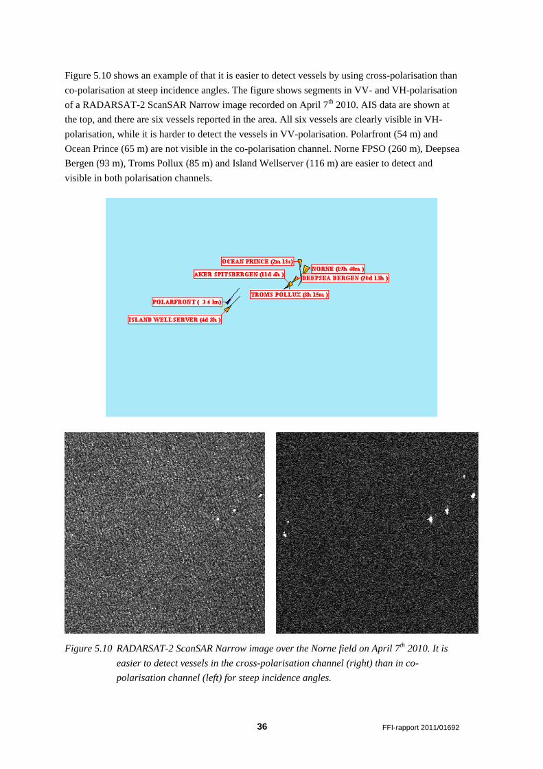
Figure 5.10 shows an example of that it is easier to detect vessels by using cross-polarisation than
co-polarisation at steep incidence angles. The figure shows segments in VV- and VH-polarisation
of a RADARSAT-2 ScanSAR Narrow image recorded on April 7th 2010. AIS data are shown at
the top, and there are six vessels reported in the area. All six vessels are clearly visible in VH-
polarisation, while it is harder to detect the vessels in VV-polarisation. Polarfront (54 m) and
Ocean Prince (65 m) are not visible in the co-polarisation channel. Norne FPSO (260 m), Deepsea
Bergen (93 m), Troms Pollux (85 m) and Island Wellserver (116 m) are easier to detect and
visible in both polarisation channels.
Figure 5.10 RADARSAT-2 ScanSAR Narrow image over the Norne field on April 7th 2010. It is
easier to detect vessels in the cross-polarisation channel (right) than in co-
polarisation channel (left) for steep incidence angles.
FFI-rapport 2011/01692 37
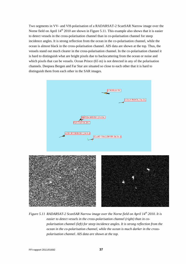
Two segments in VV- and VH-polarisation of a RADARSAT-2 ScanSAR Narrow image over the
Norne field on April 14th 2010 are shown in Figure 5.11. This example also shows that it is easier
to detect vessels in the cross-polarisation channel than in co-polarisation channel for steep
incidence angles. It is strong reflection from the ocean in the co-polarisation channel, while the
ocean is almost black in the cross-polarisation channel. AIS data are shown at the top. Thus, the
vessels stand out much clearer in the cross-polarisation channel. In the co-polarisation channel it
is hard to distinguish what are bright pixels due to backscattering from the ocean or noise and
which pixels that can be vessels. Ocean Prince (65 m) is not detected in any of the polarisation
channels. Deepsea Bergen and Far Star are situated so close to each other that it is hard to
distinguish them from each other in the SAR images.
Figure 5.11 RADARSAT-2 ScanSAR Narrow image over the Norne field on April 14th 2010. It is
easier to detect vessels in the cross-polarisation channel (right) than in co-
polarisation channel (left) for steep incidence angles. It is strong reflection from the
ocean in the co-polarisation channel, while the ocean is much darker in the cross-
polarisation channel. AIS data are shown at the top.
38 FFI-rapport 2011/01692
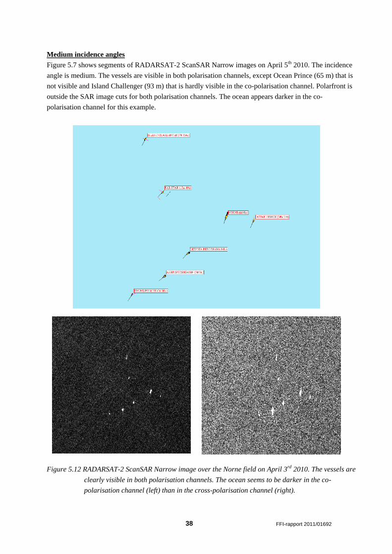
Medium incidence angles
Figure 5.7 shows segments of RADARSAT-2 ScanSAR Narrow images on April 5th 2010. The incidence
angle is medium. The vessels are visible in both polarisation channels, except Ocean Prince (65 m) that is
not visible and Island Challenger (93 m) that is hardly visible in the co-polarisation channel. Polarfront is
outside the SAR image cuts for both polarisation channels. The ocean appears darker in the co-
polarisation channel for this example.
Figure 5.12 RADARSAT-2 ScanSAR Narrow image over the Norne field on April 3rd 2010. The vessels are
clearly visible in both polarisation channels. The ocean seems to be darker in the co-
polarisation channel (left) than in the cross-polarisation channel (right).
FFI-rapport 2011/01692 39
High incidence angles
Figure 5.12 shows segments of RADARSAT-2 ScanSAR Narrow images on April 3rd 2010. The
vessels are visible in both polarisation channels, and it shows that both co- and cross-polarisation
channels can be used for ship detection for high incidence angles. The ocean is darker in the co-
polarisation channel, which makes it a little bit easier to distinguish the vessels from the ocean
background manually.
5.3.2 Quad-polarised data
When quad-polarised data are available, it is possible to either look at the polarisation channels
independently or by combining the different channels in a polarimetric analysis, which gives
information about structure and shape of different scattering surfaces. When fully-polarimetric
data are available, it is possible to get more complete information about the data.
Aegir is used to do automatic ship detection on the Norne field. Aegir is a SAR marine imagery
analysis tool developed at the Norwegian Defence Research Establishment (FFI). Two different
threshold algorithms can be used to do the automatic ship detection, N-sigma and K-distribution
[14]. The output data is polarisation, vessel size (number of pixels), peak value, target position,
estimated vessel length, estimated vessel beam, estimated heading and detection confidence. The
detected targets are plotted for the user as symbols in the SAR image (see example in Figure
5.13). The detection confidence is estimated based on the combined results from the available
bands. If AIS data are available, the AIS position can also be plotted as symbols overlaid the SAR
image. At last, a manual verification step may be done, where the user can look at all the
detections and discard or accept each of the detections.
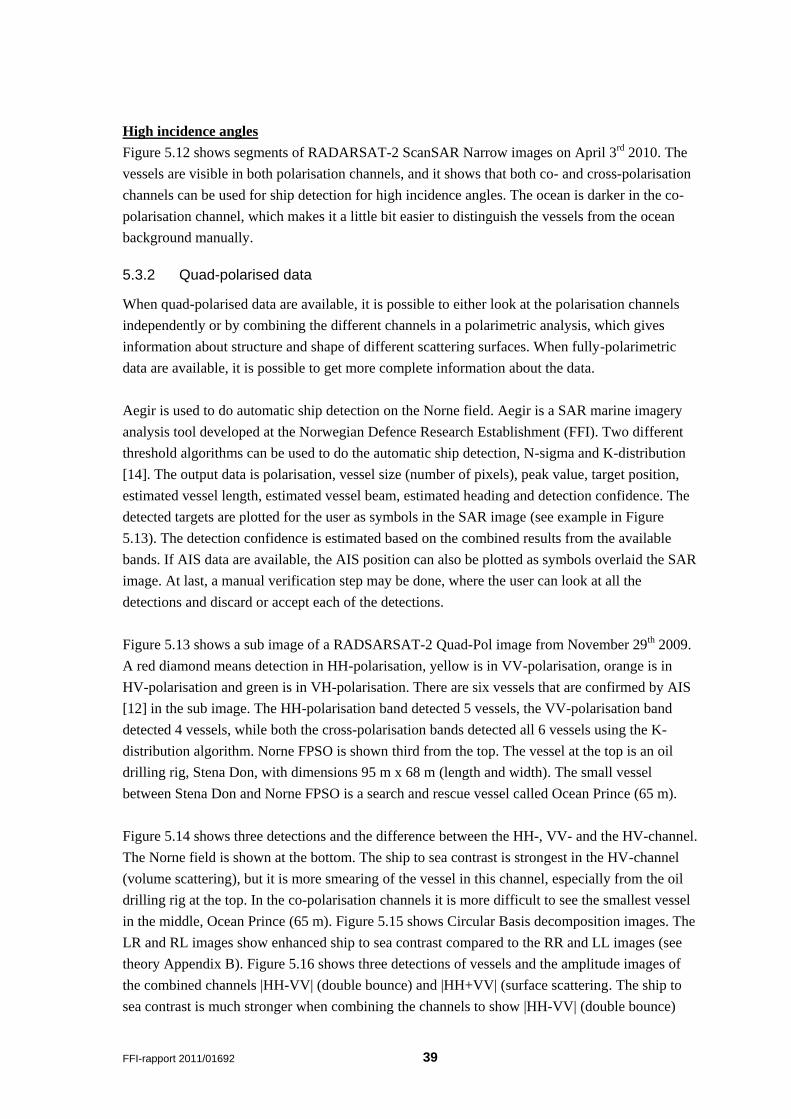
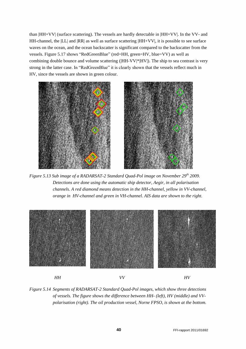
Figure 5.13 shows a sub image of a RADSARSAT-2 Quad-Pol image from November 29th 2009.
A red diamond means detection in HH-polarisation, yellow is in VV-polarisation, orange is in
HV-polarisation and green is in VH-polarisation. There are six vessels that are confirmed by AIS
[12] in the sub image. The HH-polarisation band detected 5 vessels, the VV-polarisation band
detected 4 vessels, while both the cross-polarisation bands detected all 6 vessels using the K-
distribution algorithm. Norne FPSO is shown third from the top. The vessel at the top is an oil
drilling rig, Stena Don, with dimensions 95 m x 68 m (length and width). The small vessel
between Stena Don and Norne FPSO is a search and rescue vessel called Ocean Prince (65 m).
Figure 5.14 shows three detections and the difference between the HH-, VV- and the HV-channel.
The Norne field is shown at the bottom. The ship to sea contrast is strongest in the HV-channel
(volume scattering), but it is more smearing of the vessel in this channel, especially from the oil
drilling rig at the top. In the co-polarisation channels it is more difficult to see the smallest vessel
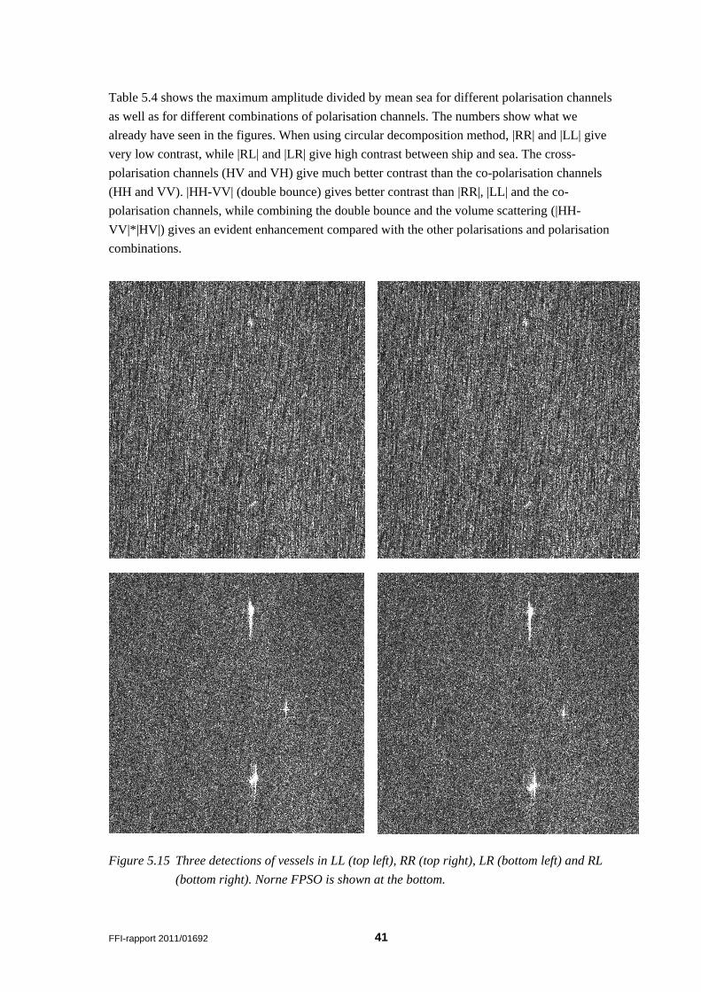
in the middle, Ocean Prince (65 m). Figure 5.15 shows Circular Basis decomposition images. The
LR and RL images show enhanced ship to sea contrast compared to the RR and LL images (see
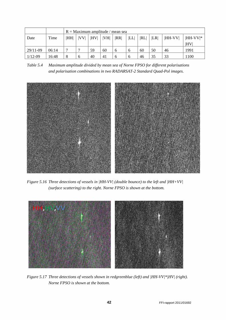
theory Appendix B). Figure 5.16 shows three detections of vessels and the amplitude images of
the combined channels |HH-VV| (double bounce) and |HH+VV| (surface scattering. The ship to
sea contrast is much stronger when combining the channels to show |HH-VV| (double bounce)
40 FFI-rapport 2011/01692
than |HH+VV| (surface scattering). The vessels are hardly detectable in |HH+VV|. In the VV- and
HH-channel, the |LL| and |RR| as well as surface scattering |HH+VV|, it is possible to see surface
waves on the ocean, and the ocean backscatter is significant compared to the backscatter from the
vessels. Figure 5.17 shows “RedGreenBlue” (red=HH, green=HV, blue=VV) as well as
combining double bounce and volume scattering (|HH-VV|*|HV|). The ship to sea contrast is very
strong in the latter case. In “RedGreenBlue” it is clearly shown that the vessels reflect much in
HV, since the vessels are shown in green colour.
Figure 5.13 Sub image of a RADARSAT-2 Standard Quad-Pol image on November 29th 2009.
Detections are done using the automatic ship detector, Aegir, in all polarisation
channels. A red diamond means detection in the HH-channel, yellow in VV-channel,
orange in HV-channel and green in VH-channel. AIS data are shown to the right.
HH VV HV
Figure 5.14 Segments of RADARSAT-2 Standard Quad-Pol images, which show three detections
of vessels. The figure shows the difference between HH- (left), HV (middle) and VV-
polarisation (right). The oil production vessel, Norne FPSO, is shown at the bottom.
FFI-rapport 2011/01692 41
Table 5.4 shows the maximum amplitude divided by mean sea for different polarisation channels
as well as for different combinations of polarisation channels. The numbers show what we
already have seen in the figures. When using circular decomposition method, |RR| and |LL| give
very low contrast, while |RL| and |LR| give high contrast between ship and sea. The cross-
polarisation channels (HV and VH) give much better contrast than the co-polarisation channels
(HH and VV). |HH-VV| (double bounce) gives better contrast than |RR|, |LL| and the co-
polarisation channels, while combining the double bounce and the volume scattering (|HH-
VV|*|HV|) gives an evident enhancement compared with the other polarisations and polarisation
combinations.
Figure 5.15 Three detections of vessels in LL (top left), RR (top right), LR (bottom left) and RL
(bottom right). Norne FPSO is shown at the bottom.
42 FFI-rapport 2011/01692
R = Maximum amplitude / mean sea
Date Time |HH| |VV| |HV| |VH| |RR| |LL| |RL| |LR| |HH-VV| |HH-VV|*
|HV|
29/11-09 06:14 7 7 59 60 6 6 60 50 46 1991
1/12-09 16:48 8 6 40 41 6 6 46 35 33 1100
Table 5.4 Maximum amplitude divided by mean sea of Norne FPSO for different polarisations
and polarisation combinations in two RADARSAT-2 Standard Quad-Pol images.
Figure 5.16 Three detections of vessels in |HH-VV| (double bounce) to the left and |HH+VV|
(surface scattering) to the right. Norne FPSO is shown at the bottom.
Figure 5.17 Three detections of vessels shown in redgreenblue (left) and |HH-VV|*|HV| (right).
Norne FPSO is shown at the bottom.
FFI-rapport 2011/01692 43
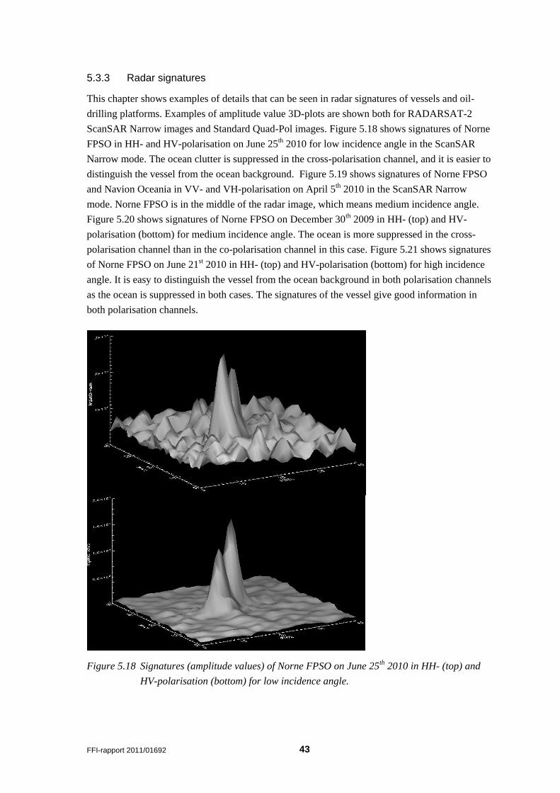
5.3.3 Radar signatures
This chapter shows examples of details that can be seen in radar signatures of vessels and oil-
drilling platforms. Examples of amplitude value 3D-plots are shown both for RADARSAT-2
ScanSAR Narrow images and Standard Quad-Pol images. Figure 5.18 shows signatures of Norne
FPSO in HH- and HV-polarisation on June 25th 2010 for low incidence angle in the ScanSAR
Narrow mode. The ocean clutter is suppressed in the cross-polarisation channel, and it is easier to
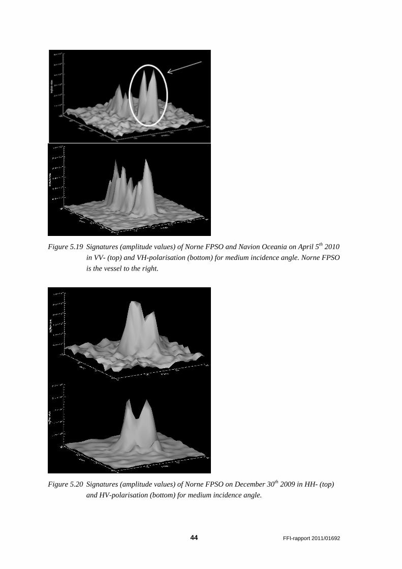
distinguish the vessel from the ocean background. Figure 5.19 shows signatures of Norne FPSO
and Navion Oceania in VV- and VH-polarisation on April 5th 2010 in the ScanSAR Narrow
mode. Norne FPSO is in the middle of the radar image, which means medium incidence angle.
Figure 5.20 shows signatures of Norne FPSO on December 30th 2009 in HH- (top) and HV-
polarisation (bottom) for medium incidence angle. The ocean is more suppressed in the cross-
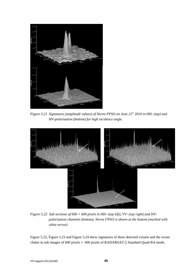
polarisation channel than in the co-polarisation channel in this case. Figure 5.21 shows signatures
of Norne FPSO on June 21st 2010 in HH- (top) and HV-polarisation (bottom) for high incidence
angle. It is easy to distinguish the vessel from the ocean background in both polarisation channels
as the ocean is suppressed in both cases. The signatures of the vessel give good information in
both polarisation channels.
Figure 5.18 Signatures (amplitude values) of Norne FPSO on June 25th 2010 in HH- (top) and
HV-polarisation (bottom) for low incidence angle.
44 FFI-rapport 2011/01692
Figure 5.19 Signatures (amplitude values) of Norne FPSO and Navion Oceania on April 5th 2010
in VV- (top) and VH-polarisation (bottom) for medium incidence angle. Norne FPSO
is the vessel to the right.
Figure 5.20 Signatures (amplitude values) of Norne FPSO on December 30th 2009 in HH- (top)
and HV-polarisation (bottom) for medium incidence angle.
FFI-rapport 2011/01692 45
Figure 5.21 Signatures (amplitude values) of Norne FPSO on June 21st 2010 in HH- (top) and
HV-polarisation (bottom) for high incidence angle.
Figure 5.22 Sub sections of 600 × 600 pixels in HH- (top left), VV- (top right) and HV-
polarisation channels (bottom). Norne FPSO is shown at the bottom (marked with
white arrow)
Figure 5.22, Figure 5.23 and Figure 5.24 show signatures of three detected vessels and the ocean
clutter in sub images of 600 pixels 600 pixels of RADARSAT-2 Standard Quad-Pol mode.
46 FFI-rapport 2011/01692
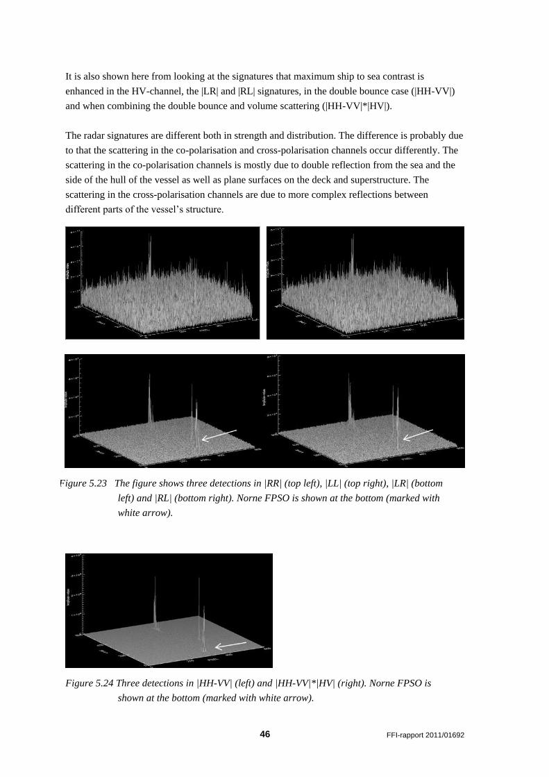
It is also shown here from looking at the signatures that maximum ship to sea contrast is
enhanced in the HV-channel, the |LR| and |RL| signatures, in the double bounce case (|HH-VV|)
and when combining the double bounce and volume scattering (|HH-VV|*|HV|).
The radar signatures are different both in strength and distribution. The difference is probably due
to that the scattering in the co-polarisation and cross-polarisation channels occur differently. The
scattering in the co-polarisation channels is mostly due to double reflection from the sea and the
side of the hull of the vessel as well as plane surfaces on the deck and superstructure. The
scattering in the cross-polarisation channels are due to more complex reflections between
different parts of the vessel’s structure.
Figure 5.23 The figure shows three detections in |RR| (top left), |LL| (top right), |LR| (bottom
left) and |RL| (bottom right). Norne FPSO is shown at the bottom (marked with
white arrow).
Figure 5.24 Three detections in |HH-VV| (left) and |HH-VV|*|HV| (right). Norne FPSO is
shown at the bottom (marked with white arrow).
FFI-rapport 2011/01692 47
6 On-going and future developments
6.1 RADARSAT Constellation Mission
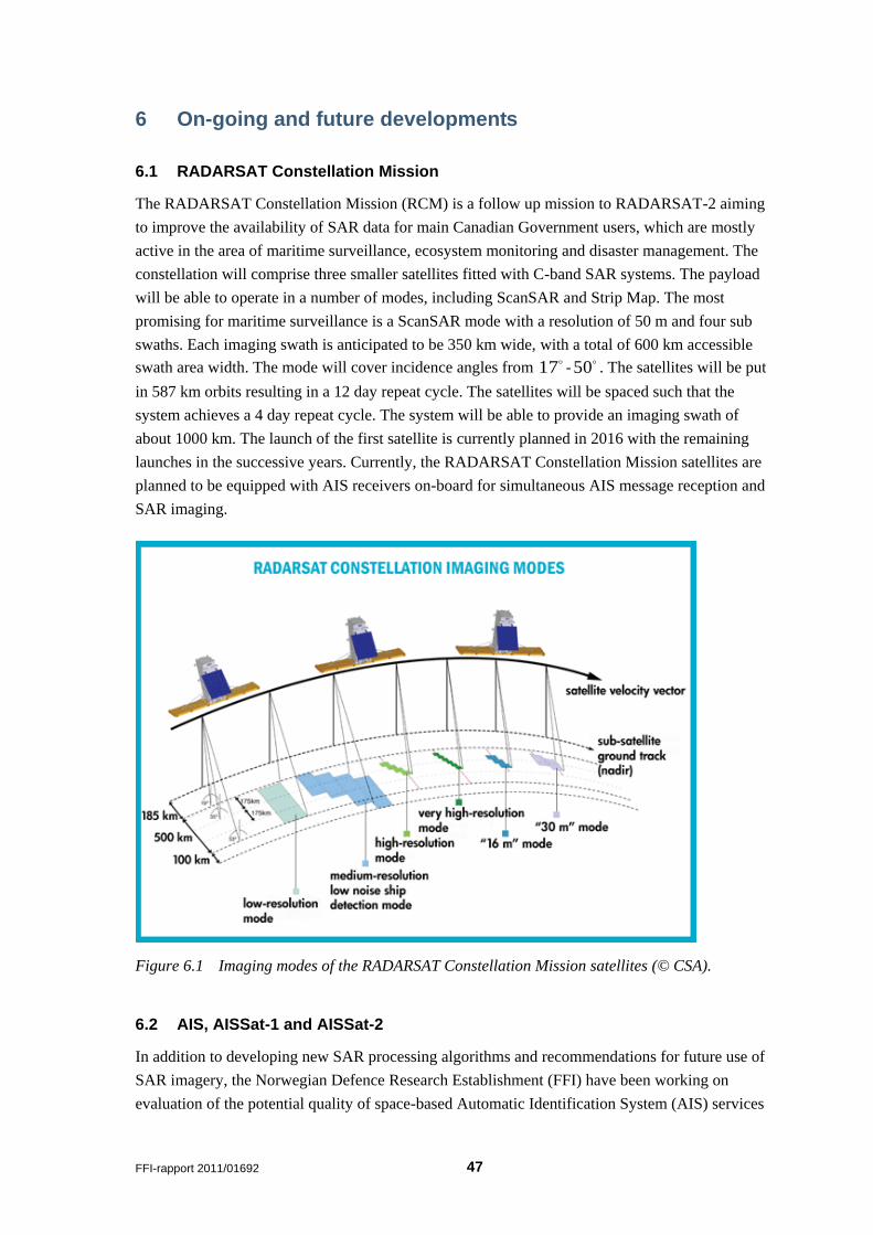
The RADARSAT Constellation Mission (RCM) is a follow up mission to RADARSAT-2 aiming
to improve the availability of SAR data for main Canadian Government users, which are mostly
active in the area of maritime surveillance, ecosystem monitoring and disaster management. The
constellation will comprise three smaller satellites fitted with C-band SAR systems. The payload
will be able to operate in a number of modes, including ScanSAR and Strip Map. The most
promising for maritime surveillance is a ScanSAR mode with a resolution of 50 m and four sub
swaths. Each imaging swath is anticipated to be 350 km wide, with a total of 600 km accessible
swath area width. The mode will cover incidence angles from 17 -
50 . The satellites will be put
in 587 km orbits resulting in a 12 day repeat cycle. The satellites will be spaced such that the
system achieves a 4 day repeat cycle. The system will be able to provide an imaging swath of
about 1000 km. The launch of the first satellite is currently planned in 2016 with the remaining
launches in the successive years. Currently, the RADARSAT Constellation Mission satellites are
planned to be equipped with AIS receivers on-board for simultaneous AIS message reception and
SAR imaging.
Figure 6.1 Imaging modes of the RADARSAT Constellation Mission satellites (© CSA).
6.2 AIS, AISSat-1 and AISSat-2
In addition to developing new SAR processing algorithms and recommendations for future use of
SAR imagery, the Norwegian Defence Research Establishment (FFI) have been working on
evaluation of the potential quality of space-based Automatic Identification System (AIS) services
48 FFI-rapport 2011/01692
[15;16]. The AIS is a ship-to-shore system as well as a ship-to-ship anti-collision system of
shipboard transponders that automatically exchange vessel traffic information for maritime safety,
mandated by the International Maritime Organisation (IMO) on larger vessels. All passenger
ships, cargo ships over 300 gross tons and all fishing vessels over 45 meters must have an AIS
transponder onboard the ship. Information obtained from the AIS system is the ship’s position,
speed, heading, load, size, ship type and more. AIS signals sent from the land-based stations have
a range of 40 nautical miles. A satellite-based AIS system will increase this range tremendously
to cover larger ocean areas, thus making it easier to monitor the vast ocean areas in the High
North, which are difficult to monitor with the land-based AIS network that exists today.
Operationally, vessel tracking based on SAR and AIS will give a picture of all vessels in the area.
Ship detection in SAR imagery and tracking based on AIS reports are complementary. SAR and
AIS can be combined for surveillance in remote areas. AIS information can identify vessels
detected in SAR images, while SAR can be used to detect vessels not reporting through AIS. The
combination of sources gives the opportunity to unveil vessels that don’t send mandatory AIS
reports.
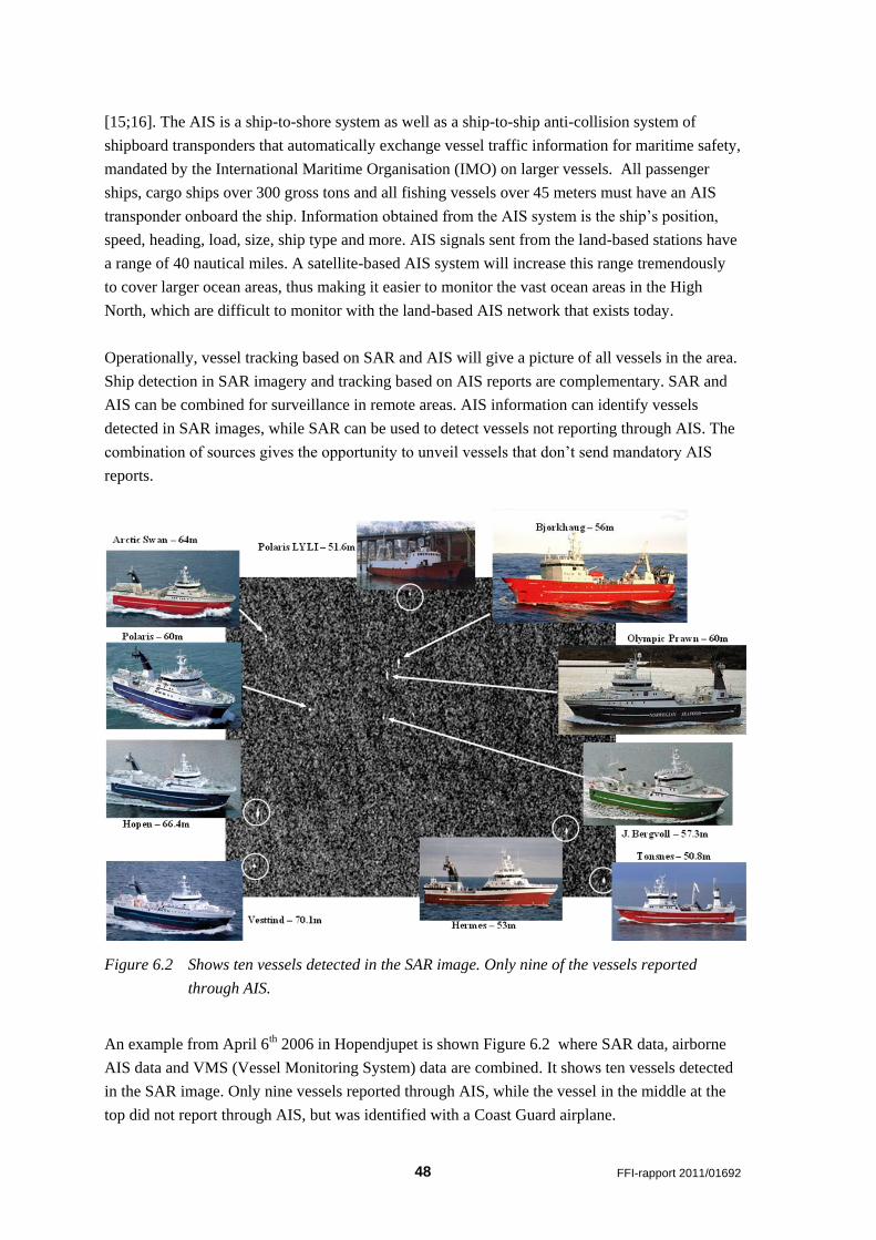
Figure 6.2 Shows ten vessels detected in the SAR image. Only nine of the vessels reported
through AIS.
An example from April 6th 2006 in Hopendjupet is shown Figure 6.2 where SAR data, airborne
AIS data and VMS (Vessel Monitoring System) data are combined. It shows ten vessels detected
in the SAR image. Only nine vessels reported through AIS, while the vessel in the middle at the
top did not report through AIS, but was identified with a Coast Guard airplane.
FFI-rapport 2011/01692 49
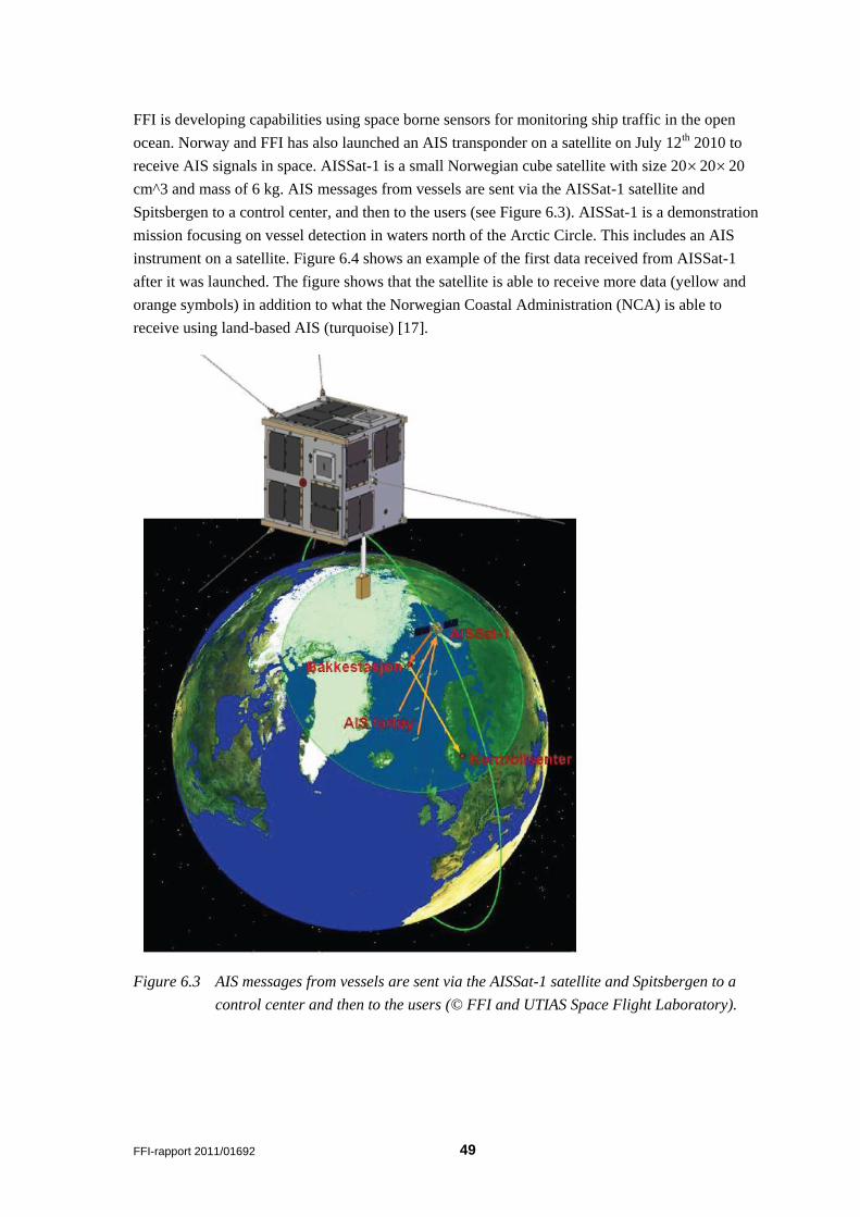
FFI is developing capabilities using space borne sensors for monitoring ship traffic in the open
ocean. Norway and FFI has also launched an AIS transponder on a satellite on July 12th 2010 to
receive AIS signals in space. AISSat-1 is a small Norwegian cube satellite with size 202020
cm^3 and mass of 6 kg. AIS messages from vessels are sent via the AISSat-1 satellite and
Spitsbergen to a control center, and then to the users (see Figure 6.3). AISSat-1 is a demonstration
mission focusing on vessel detection in waters north of the Arctic Circle. This includes an AIS
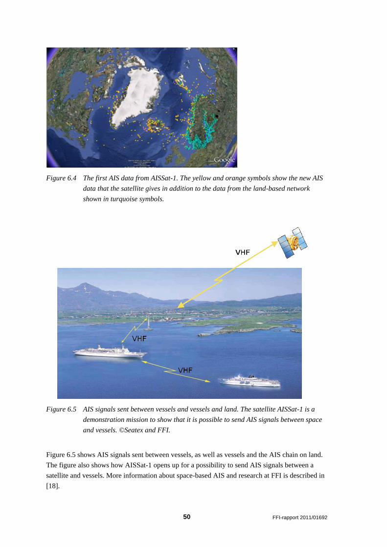
instrument on a satellite. Figure 6.4 shows an example of the first data received from AISSat-1
after it was launched. The figure shows that the satellite is able to receive more data (yellow and
orange symbols) in addition to what the Norwegian Coastal Administration (NCA) is able to
receive using land-based AIS (turquoise) [17].
Figure 6.3 AIS messages from vessels are sent via the AISSat-1 satellite and Spitsbergen to a
control center and then to the users (© FFI and UTIAS Space Flight Laboratory).
50 FFI-rapport 2011/01692
Figure 6.4 The first AIS data from AISSat-1. The yellow and orange symbols show the new AIS
data that the satellite gives in addition to the data from the land-based network
shown in turquoise symbols.
Figure 6.5 AIS signals sent between vessels and vessels and land. The satellite AISSat-1 is a
demonstration mission to show that it is possible to send AIS signals between space
and vessels. ©Seatex and FFI.
Figure 6.5 shows AIS signals sent between vessels, as well as vessels and the AIS chain on land.
The figure also shows how AISSat-1 opens up for a possibility to send AIS signals between a
satellite and vessels. More information about space-based AIS and research at FFI is described in
[18].
FFI-rapport 2011/01692 51
AISSat-2 is a follow-up mission after AISSat-1, and will be Norway’s second satellite. It will be
almost identical to AISSat-1, but with some small adjustments where it is useful. The satellite will
provide increased coverage and will be a back-up to AISSat-1. The launch is planned in 2012.
The AISSat-3 mission is in an early planning phase, and will be a follow-up after AISSat-1 and
AISSat-2. AISSat-3 will have some changes compared to its predecessors, for example some new
instruments, and will be a next generation AIS satellite. The building is planned to start in 2012
[19].
7 Conclusion
RADARSAT-2 provides new opportunities for spaceborne monitoring of vessel traffic and
fishing activities. The satellite has better resolution than earlier radar satellites, flexible look
direction and multiple polarisation options.
RADARSAT-2 gives good opportunities to effectively monitor large ocean areas. By using the
ScanSAR modes it is possible to cover an area of 300 km x 300 km for the ScanSAR Narrow
mode and 500 km x 500 km for the ScanSAR Wide mode [1]. In good conditions the resolution
these modes gives is sufficient to give information about:
- Detection
- Position
- Rough size estimate of the vessel
Earlier advice has been to use large incidence angles and HH-polarisation to detect ships. When
ENVISAT Alternating Polarisation mode data became available, we demonstrated that cross-
polarised data can be used for ship detection at low incidence angles.
A series of RADARSAT-2 data has been collected over Norwegian waters to do further analyses
on mode selection and polarisation combinations on RADARSAT-2. Both ScanSAR and
Standard Quad-Pol images have been used in the analyses. The Norne field was used as a test site,
because it is possible to image the same vessel, the oil production vessel Norne FPSO, under
different conditions, incidence angles and modes.
The information in dual-polarised is not as complete as in fully-polarimetric data sets, but it gives
some enhancements compared to using single polarisation. It is possible to get information by
looking at the channels separately and also by combining the two channels. The ship to sea
contrast is enhanced significantly combining the two channels.
When quad-polarised data are available, it is possible to combine the information from the
different polarisation channels. Multiplying the double bounce by the volume scattering shows
significant improvements in the maximum ship to sea contrast for Norne FPSO.
52 FFI-rapport 2011/01692
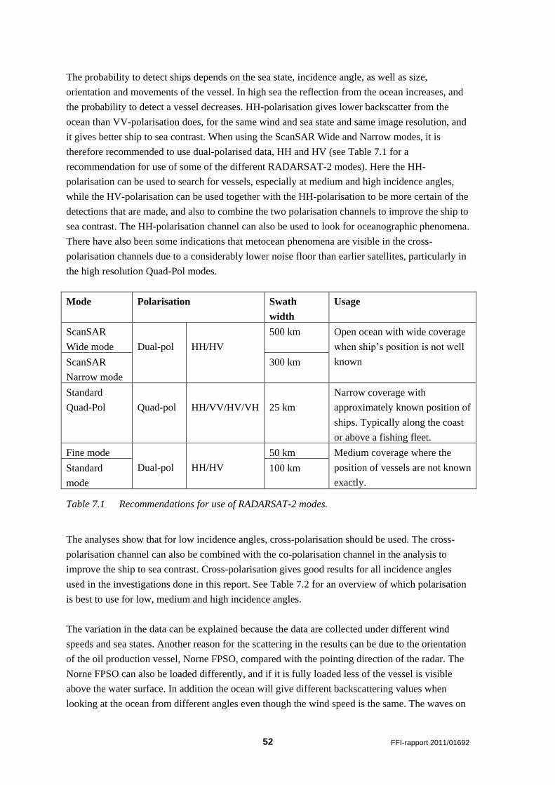
The probability to detect ships depends on the sea state, incidence angle, as well as size,
orientation and movements of the vessel. In high sea the reflection from the ocean increases, and
the probability to detect a vessel decreases. HH-polarisation gives lower backscatter from the
ocean than VV-polarisation does, for the same wind and sea state and same image resolution, and
it gives better ship to sea contrast. When using the ScanSAR Wide and Narrow modes, it is
therefore recommended to use dual-polarised data, HH and HV (see Table 7.1 for a
recommendation for use of some of the different RADARSAT-2 modes). Here the HH-
polarisation can be used to search for vessels, especially at medium and high incidence angles,
while the HV-polarisation can be used together with the HH-polarisation to be more certain of the
detections that are made, and also to combine the two polarisation channels to improve the ship to
sea contrast. The HH-polarisation channel can also be used to look for oceanographic phenomena.
There have also been some indications that metocean phenomena are visible in the cross-
polarisation channels due to a considerably lower noise floor than earlier satellites, particularly in
the high resolution Quad-Pol modes.
Mode Polarisation Swath
width
Usage
ScanSAR
Wide mode
Dual-pol
HH/HV
500 km Open ocean with wide coverage
when ship’s position is not well
known ScanSAR
Narrow mode
300 km
Standard
Quad-Pol
Quad-pol
HH/VV/HV/VH
25 km
Narrow coverage with
approximately known position of
ships. Typically along the coast
or above a fishing fleet.
Fine mode
Dual-pol
HH/HV
50 km Medium coverage where the
position of vessels are not known
exactly.
Standard
mode
100 km
Table 7.1 Recommendations for use of RADARSAT-2 modes.
The analyses show that for low incidence angles, cross-polarisation should be used. The cross-
polarisation channel can also be combined with the co-polarisation channel in the analysis to
improve the ship to sea contrast. Cross-polarisation gives good results for all incidence angles
used in the investigations done in this report. See Table 7.2 for an overview of which polarisation
is best to use for low, medium and high incidence angles.
The variation in the data can be explained because the data are collected under different wind
speeds and sea states. Another reason for the scattering in the results can be due to the orientation
of the oil production vessel, Norne FPSO, compared with the pointing direction of the radar. The
Norne FPSO can also be loaded differently, and if it is fully loaded less of the vessel is visible
above the water surface. In addition the ocean will give different backscattering values when
looking at the ocean from different angles even though the wind speed is the same. The waves on
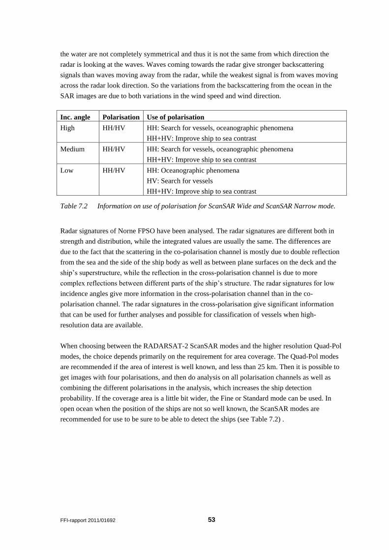
FFI-rapport 2011/01692 53
the water are not completely symmetrical and thus it is not the same from which direction the
radar is looking at the waves. Waves coming towards the radar give stronger backscattering
signals than waves moving away from the radar, while the weakest signal is from waves moving
across the radar look direction. So the variations from the backscattering from the ocean in the
SAR images are due to both variations in the wind speed and wind direction.
Inc. angle Polarisation Use of polarisation
High HH/HV HH: Search for vessels, oceanographic phenomena
HH+HV: Improve ship to sea contrast
Medium HH/HV HH: Search for vessels, oceanographic phenomena
HH+HV: Improve ship to sea contrast
Low HH/HV HH: Oceanographic phenomena
HV: Search for vessels
HH+HV: Improve ship to sea contrast
Table 7.2 Information on use of polarisation for ScanSAR Wide and ScanSAR Narrow mode.
Radar signatures of Norne FPSO have been analysed. The radar signatures are different both in
strength and distribution, while the integrated values are usually the same. The differences are
due to the fact that the scattering in the co-polarisation channel is mostly due to double reflection
from the sea and the side of the ship body as well as between plane surfaces on the deck and the
ship’s superstructure, while the reflection in the cross-polarisation channel is due to more
complex reflections between different parts of the ship’s structure. The radar signatures for low
incidence angles give more information in the cross-polarisation channel than in the co-
polarisation channel. The radar signatures in the cross-polarisation give significant information
that can be used for further analyses and possible for classification of vessels when high-
resolution data are available.
When choosing between the RADARSAT-2 ScanSAR modes and the higher resolution Quad-Pol
modes, the choice depends primarily on the requirement for area coverage. The Quad-Pol modes
are recommended if the area of interest is well known, and less than 25 km. Then it is possible to
get images with four polarisations, and then do analysis on all polarisation channels as well as
combining the different polarisations in the analysis, which increases the ship detection
probability. If the coverage area is a little bit wider, the Fine or Standard mode can be used. In
open ocean when the position of the ships are not so well known, the ScanSAR modes are
recommended for use to be sure to be able to detect the ships (see Table 7.2) .
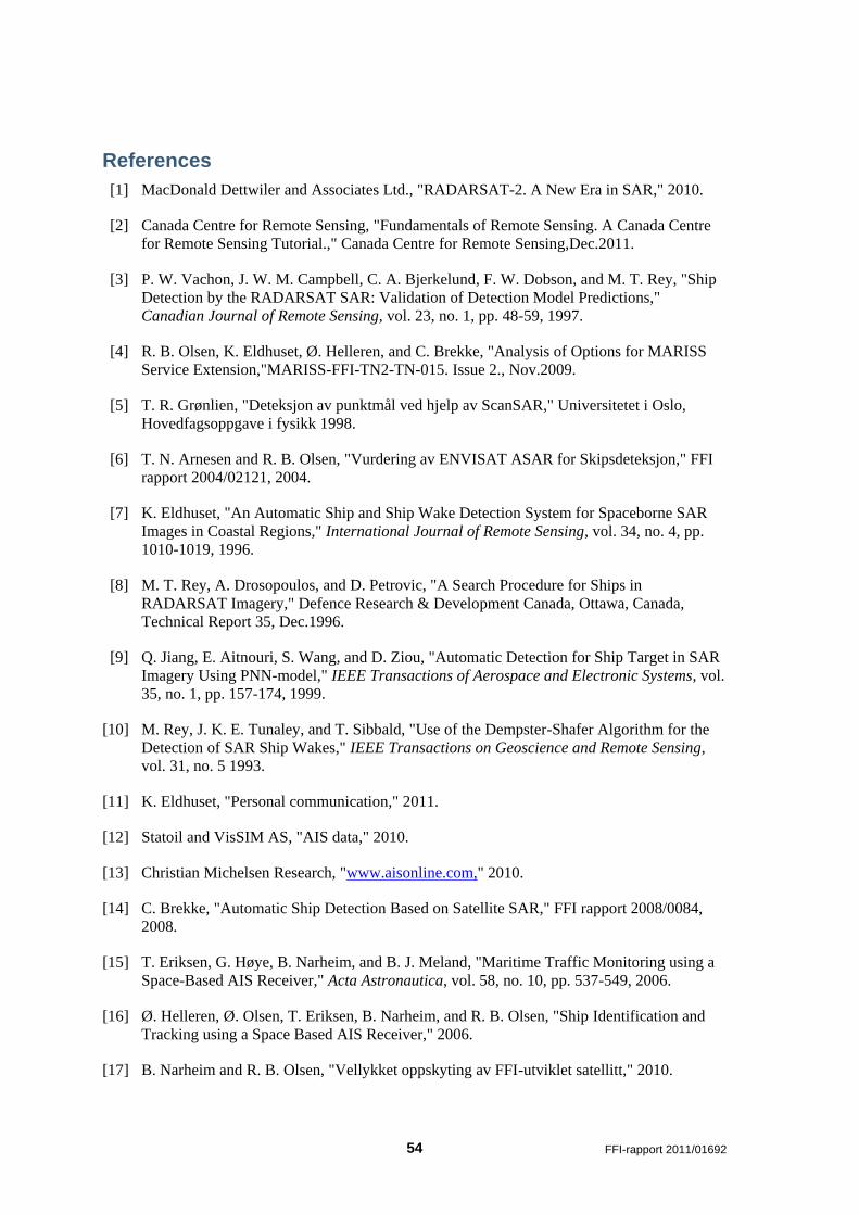
54 FFI-rapport 2011/01692
References
[1] MacDonald Dettwiler and Associates Ltd., "RADARSAT-2. A New Era in SAR," 2010.
[2] Canada Centre for Remote Sensing, "Fundamentals of Remote Sensing. A Canada Centre
for Remote Sensing Tutorial.," Canada Centre for Remote Sensing,Dec.2011.
[3] P. W. Vachon, J. W. M. Campbell, C. A. Bjerkelund, F. W. Dobson, and M. T. Rey, "Ship
Detection by the RADARSAT SAR: Validation of Detection Model Predictions,"
Canadian Journal of Remote Sensing, vol. 23, no. 1, pp. 48-59, 1997.
[4] R. B. Olsen, K. Eldhuset, Ø. Helleren, and C. Brekke, "Analysis of Options for MARISS
Service Extension,"MARISS-FFI-TN2-TN-015. Issue 2., Nov.2009.
[5] T. R. Grønlien, "Deteksjon av punktmål ved hjelp av ScanSAR," Universitetet i Oslo,
Hovedfagsoppgave i fysikk 1998.
[6] T. N. Arnesen and R. B. Olsen, "Vurdering av ENVISAT ASAR for Skipsdeteksjon," FFI
rapport 2004/02121, 2004.
[7] K. Eldhuset, "An Automatic Ship and Ship Wake Detection System for Spaceborne SAR
Images in Coastal Regions," International Journal of Remote Sensing, vol. 34, no. 4, pp.
1010-1019, 1996.
[8] M. T. Rey, A. Drosopoulos, and D. Petrovic, "A Search Procedure for Ships in
RADARSAT Imagery," Defence Research & Development Canada, Ottawa, Canada,
Technical Report 35, Dec.1996.
[9] Q. Jiang, E. Aitnouri, S. Wang, and D. Ziou, "Automatic Detection for Ship Target in SAR
Imagery Using PNN-model," IEEE Transactions of Aerospace and Electronic Systems, vol.
35, no. 1, pp. 157-174, 1999.
[10] M. Rey, J. K. E. Tunaley, and T. Sibbald, "Use of the Dempster-Shafer Algorithm for the
Detection of SAR Ship Wakes," IEEE Transactions on Geoscience and Remote Sensing,
vol. 31, no. 5 1993.
[11] K. Eldhuset, "Personal communication," 2011.
[12] Statoil and VisSIM AS, "AIS data," 2010.
[13] Christian Michelsen Research, "www.aisonline.com," 2010.
[14] C. Brekke, "Automatic Ship Detection Based on Satellite SAR," FFI rapport 2008/0084,
2008.
[15] T. Eriksen, G. Høye, B. Narheim, and B. J. Meland, "Maritime Traffic Monitoring using a
Space-Based AIS Receiver," Acta Astronautica, vol. 58, no. 10, pp. 537-549, 2006.
[16] Ø. Helleren, Ø. Olsen, T. Eriksen, B. Narheim, and R. B. Olsen, "Ship Identification and
Tracking using a Space Based AIS Receiver," 2006.
[17] B. Narheim and R. B. Olsen, "Vellykket oppskyting av FFI-utviklet satellitt," 2010.
FFI-rapport 2011/01692 55
[18] T. Eriksen, A. N. Skauen, B. Narheim, Ø. Helleren, Ø. Olsen, and R. B. Olsen, "Tracking
Ship Traffic with Space-Based AIS. Experience Gained in the First Months of Operations. "
2010.
[19] Norsk Romsenter, "www.romsenter.no," 2011.
[20] Y. Yamaguchi, A. Sato, W.-M. Boerner, R. Sato, and H. Yamada, "Four-Component
Scattering Power Decomposition with Rotation of Coherency Matrix," IEEE Transactions
on Geoscience and Remote Sensing, vol. 49, no. 6 2011.
56 FFI-rapport 2011/01692
Acronyms
AIS Automatic Identification System
AP Alternating Polarisation
ASAR Advanced Synthetic Aperture Radar
CCRS Canada Centre for Remote Sensing
CFAR Constant False Alarm Rate
CSA Canadian Space Agency
ERS European Remote Sensing
Dual-pol Dual-polarisation
EH Extended High
EL Extended Low
ESA European Space Agency
F Fine
FFI Forsvarets Forskningsinstitutt
H Horisontal polarisation
HH Horisontally transmitted – Horisontally received polarisation
HV Horisontally transmitted – Vertically received polarisation
i Inclination
IDL Interactive Data Language
IMO International Maritime Organisation
KSAT Kongsberg Satellite Services AS
MDA MacDonald, Dettwiler and Associates Ltd
MF Multi-Look Fine
PDF Probability Density Function
Pol Polarisation
Quad-pol Quad-polarisation
RCM Radarsat Constellation Mission
RCS Radar Cross Section
S Standard
SAR Synthetic Aperture Radar
SCN ScanSAR Narrow
SCW ScanSAR Wide
SLC Single Look Complex
TCR Target to Clutter Ratio
V Vertical polarisation
VH Vertically transmitted – Horisontally received polarisation
VMS Vessel Monitoring System
VV Vertically transmitted – Vertically received polarisation
W Wide
FFI-rapport 2011/01692 57
Appendix A Pauli Decomposition
One well known polarimetric decomposition method is the Pauli decomposition, which gives
components of surface scattering (|HH+VV|), volume scattering (|HV| or |VH|) and double
bounce (|HH-VV|). An example is shown in Figure 4.2 where six vessels in the Norne field are
shown. They appear as brighter targets compared to the ocean background. The oil production
vessel, Norne FPSO, is shown third from the top. The three different components are displayed in
different colours, and two scaling factors can be used, sc1 = 0.7 and sc2 = 2. The surface
scattering is odd bounce (surface, sphere or corner reflector), displayed in blue and scaled with
scaling factor sc1: (HH+VV) ^ 0.7. The double bounce is even bounce (dihedral or double
bounce), displayed in red and scaled with scaling factor sc1: (HH-VV) ^ 0.7. The volume
scattering is even bounce (i.e. dihedral tilted 45 degrees), displayed in green and scaled with both
scaling factors: ( 2 *(HV+VH)) ^ 0.7.
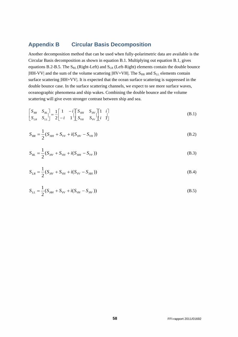
58 FFI-rapport 2011/01692
Appendix B Circular Basis Decomposition
Another decomposition method that can be used when fully-polarimetric data are available is the
Circular Basis decomposition as shown in equation B.1. Multiplying out equation B.1, gives
equations B.2-B.5. The SRL (Right-Left) and SLR (Left-Right) elements contain the double bounce
|HH-VV| and the sum of the volume scattering |HV+VH|. The SRR and SLL elements contain
surface scattering |HH+VV|. It is expected that the ocean surface scattering is suppressed in the
double bounce case. In the surface scattering channels, we expect to see more surface waves,
oceanographic phenomena and ship wakes. Combining the double bounce and the volume
scattering will give even stronger contrast between ship and sea.
1
1
1
1
2
1
i
i
SS
SS
i
i
SS
SS
VVVH
HVHH
LLLR
RLRR (B.1)
))((2
1VHHVVVHHRR SSiSSS (B.2)
))((2
1VVHHVHHVRL SSiSSS (B.3)
))((2
1HHVVVHHVLR SSiSSS (B.4)
))((2
1HVVHVVHHLL SSiSSS (B.5)
FFI-rapport 2011/01692 59
Appendix C Yamaguchi Decomposition
Yamaguchi provided a new decomposition method in [20] in 2011. To minimize the cross-
polarised component the method uses a rotation of the coherency matrix. The coherency matrix is
rotated by using the recovered angle. Then the four-component scattering power decomposition
method is applied to the four fully polarimetric SAR images. Only the coherency matrix elements
are used in this decomposition algorithm. The method is simple and effective, and it makes it
possible to discriminate between different scattering objects that were previously difficult to
discriminate, for example oriented urban blocks versus vegetation. It might be interesting to see if
this algorithm can be used for ship detection.