A part of this paper was circulated under the title “Spurious Inference in Unidentified Asset-Pricing Models.” The authors thank Seung Ahn, Alex Horenstein, Lei Jiang, Robert Kimmel, Frank Kleibergen, Francisco Peñaranda, Enrique Sentana, Chu Zhang, seminar participants at Bocconi University, EDHEC, ESSEC, Federal Reserve Bank of New York, Boston University, Hong Kong University of Science and Technology, National University of Singapore, Queen Mary University of London, University of California-San Diego, University of Cantabria, University of Exeter, University of Geneva, University of Hong Kong, University of Lugano, University of Reading, University of Rome Tor Vergata, University of Southampton, Vanderbilt University, and Western University, as well as conference participants at the 2013 All-Georgia Finance Conference, the 2013 Metro-Atlanta Econometric Study Group Meeting, the 2013 Seventh International Conference on Computational and Financial Econometrics, the 2014 China International Conference in Finance, the 2014 NBER-NSF Time-Series Conference, the 2014 Northern Finance Association Conference, the 2014 SoFiE Conference, the 2014 Tsinghua Finance Workshop, the 2015 Brunel Workshop in Empirical Finance, the 2015 Toulouse Financial Econometrics Conference, and the 2015 York Conference on Macroeconomic, Financial, and International Linkages for helpful discussions and comments. The views expressed here are the authors’ and not necessarily those of the Federal Reserve Bank of Atlanta or the Federal Reserve System. Any remaining errors are the authors’ responsibility. Please address questions regarding content to corresponding author: Nikolay Gospodinov, Research Department, Federal Reserve Bank of Atlanta, 1000 Peachtree Street NE, Atlanta, GA 30309, 404-498-7892, nikolay.gospodinov@atl.frb.org; Raymond Kan, Rotman School of Management, University of Toronto, 105 St. George Street, Toronto, Ontario M5S 3E6, Canada, kan@chass.utoronto.ca; or Cesare Robotti, Department of Finance, Terry College of Business, University of Georgia, B328 Amos Hall, 620 South Lumpkin Street, Athens, GA 30602, robotti@uga.edu. Federal Reserve Bank of Atlanta working papers, including revised versions, are available on the Atlanta Fed’s website at www.frbatlanta.org. Click “Publications” and then “Working Papers.” To receive e-mail notifications about new papers, use frbatlanta.org/forms/subscribe.

FEDERAL RESERVE BANK of ATLANTA WORKING PAPER SERIES

Too Good to Be True? Fallacies in Evaluating Risk Factor Models

Nikolay Gospodinov, Raymond Kan, and Cesare Robotti Working Paper 2017-9 November 2017 Abstract: This paper is concerned with statistical inference and model evaluation in possibly misspecified and unidentified linear asset-pricing models estimated by maximum likelihood and one-step generalized method of moments. Strikingly, when spurious factors (that is, factors that are uncorrelated with the returns on the test assets) are present, the models exhibit perfect fit, as measured by the squared correlation between the model's fitted expected returns and the average realized returns. Furthermore, factors that are spurious are selected with high probability, while factors that are useful are driven out of the model. Although ignoring potential misspecification and lack of identification can be very problematic for models with macroeconomic factors, empirical specifications with traded factors (e.g., Fama and French, 1993, and Hou, Xue, and Zhang, 2015) do not suffer of the identification problems documented in this study. JEL classification: G12, C12, C13 Key words: asset pricing, spurious risk factors, unidentified models, model misspecification, continuously updated GMM, maximum likelihood, goodness-of-fit, rank test

1 Introduction and Motivation

The search for (theoretically justified or empirically motivated) risk factors that improve the pricing

performance of various asset-pricing models has generated a large, and constantly growing, litera-

ture in financial economics. A typical empirical strategy involves the development of a structural

asset-pricing model and the evaluation of the pricing ability of the proposed factors in the linearized

version of the model using actual data. The resulting linear asset-pricing model can be estimated

and tested using a beta representation or, alternatively, a linear stochastic discount factor (SDF)

representation. Given the appealing efficiency and invariance properties of the maximum likelihood

(ML) and continuously-updated generalized method of moments (CU-GMM) estimators,1 it seems

natural to opt for these estimators when conducting statistical inference (estimation, testing, and

model evaluation) in these linear asset-pricing models. It is often the case that a high correlation

between the realized and fitted expected returns (in the beta representation framework) or statis-

tically small model pricing errors (in the SDF framework) appear to be sufficient for the applied

researcher to conclude that the model is well specified and proceed with testing for statistical sig-

nificance of the risk premium parameters using the standard tools for inference. Many asset-pricing

studies have followed this empirical strategy and collectively, the literature has identified a large

set of macroeconomic and financial factors (see Harvey, Liu, and Zhu, 2016, and Feng, Giglio, and

Xiu, 2017) that are believed to explain the cross-sectional variation of various portfolio returns,

such as the returns on the 25 Fama-French size and book-to-market ranked portfolios.

Despite these advances in the asset-pricing literature, two observations that consistently emerge

in empirical work might call for a more cautious approach to statistical validation and economic

interpretation of asset-pricing models. First, all asset-pricing models should be viewed only as

approximations to reality and, hence, potentially misspecified. There is plenty of empirical evidence,

mainly based on non-invariant estimators, which suggests that the asset-pricing models used in

practice are misspecified. This raises the concern of using standard errors, derived under the

assumption of correct model specification, that tend to underestimate the degree of uncertainty

that the researcher faces. Second, the macroeconomic factors in several asset-pricing specifications

tend to be only weakly correlated with the portfolio returns. As a result, it is plausible to conjecture

1See, for example, Shanken and Zhou (2007), Almeida and Garcia (2012, 2017), Penaranda and Sentana (2015),Manresa, Penaranda, and Sentana (2017), Barillas and Shanken (2017a, 2017b), and Ghosh, Julliard, and Taylor(2017) for some recent results on the ML and CU-GMM estimators for asset-pricing models.

1

that many of these macroeconomic factors may be irrelevant for pricing and explaining the cross-

sectional variation in stock expected returns. Importantly, the inclusion of spurious factors (that

is, factors that are uncorrelated with the returns on the test assets) leads to serious identification

issues regarding the parameters associated with all risk factors and gives rise to a non-standard

statistical inference (see, for instance, Gospodinov, Kan, and Robotti, 2014).

Under standard regularity conditions (that include global and local identification as well as

correct model specification), the ML and CU-GMM estimators considered here, which are invari-

ant to data scaling, reparameterizations and normalizations, etc. (Hall, 2005), are asymptotically

well-behaved and efficient. However, we show in this paper that in the presence of spurious factors,

the tests and goodness-of-fit measures based on these estimators could be highly misleading. In

summary, we argue that the standard inference procedures based on the ML and CU-GMM estima-

tors lead to spurious results that suggest that the model is correctly specified and the risk premium

parameters are highly significant (that is, the risk factors are priced) when, in fact, the model

is misspecified and the factors are irrelevant. The distorted nature of these results bears strong

similarities to spurious regressions with nonstationary data (Granger and Newbold, 1974, among

many others). Phillips (1989) makes an analogous observation regarding the estimators in partially

identified (albeit correctly specified) linear structural models and time series spurious regressions.

Phillips (1989, p. 201) points out that “both regressions share a fundamental indeterminacy” due

to a contaminated signal arising from either lack of identification or strength of the noise compo-

nent. We show that allowing for model misspecification further exacerbates the spuriousness of the

results and renders them completely unreliable.

To illustrate the seriousness of the problem, we start with some numerical evidence on the widely

studied static capital asset-pricing model (CAPM) with the market excess return (the return on

the value-weighted NYSE-AMEX-NASDAQ stock market index in excess of the one-month T-bill

rate, vw) as a risk factor. The test asset returns are the monthly gross returns on the popular

value-weighted 25 Fama-French size and book-to-market ranked portfolios from January 1967 until

December 2012.2

2The results that we report in this section are largely unchanged when we augment the 25 Fama-French portfolioreturns with additional test asset returns (for example, the 17 Fama-French industry portfolio returns) as recom-mended by Lewellen, Nagel, and Shanken (2010).

2

Table 1 about here

The first column of Table 1 reports some conventional statistics for evaluating the performance

of the model over this sample period both in the SDF (using CU-GMM, Panel A) and beta-pricing

(using ML, Panel B) frameworks. The statistics include tests of correct model specification (Hansen,

Heaton, and Yaron’s (1996) over-identifying restrictions test, J , for CU-GMM and Shanken’s

(1985) Wald-type test, S, for ML), the t-statistics of statistical significance constructed using

standard errors that assume correct model specification, and the pseudo-R2s computed as the

squared correlation between the fitted expected returns and average returns. In line with the results

reported elsewhere in the literature, the market factor appears to be priced with a statistically

significant risk premium. Also, consistent with the existing studies, the CAPM model is rejected

by the data. This requires the use of misspecification-robust standard errors in constructing the

t-statistics (see Gospodinov, Kan, and Robotti, 2017a). Finally, the pseudo-R2 points to some, but

not particularly strong, explanatory power.

We now add a factor, which we call the “sp” factor, to the CAPM model and, for the time

being, we do not reveal its identity and construction method. It is important to stress that the

test assets, the sample period, and the market factor remain unchanged: the only change is the

addition of the “sp” factor to the model. The results from this specification of the model are

presented in the third column (CAPM + “sp” factor) of Panels A and B in Table 1. Interestingly,

the specification tests now suggest that the model is correctly specified. Even more strikingly,

the pseudo-R2 jumps from 22.77% to 99.28% in the SDF model estimated by CU-GMM and from

14.47% to 99.99% in the beta-pricing model estimated by ML. The sp factor is highly statistically

significant while the market factor becomes insignificant. An applied researcher who is interested

in selecting parsimonious statistical models may want to remove the market factor and re-estimate

the model with the “sp” factor only.

The results from this third specification are reported in the last column of Panels A and B

in Table 1. The results are striking. First, this one-factor model exhibits an almost perfect fit

(R2 ≈ 1). Based on the specification tests, the model appears to be correctly specified. Finally,

the “sp” factor is highly statistically significant and is deemed to be priced. Given this exceptional

performance of the model, we now ask “What is this “sp” factor?” It turns out that this factor is

generated as a standard normal random variable which is independent of returns! The results of this

3

numerical exercise are completely spurious since the “sp” factor does not contribute to pricing by

construction. In summary, an arbitrarily bad model with one or more spurious factors is concluded

to be a correctly specified model with a spectacular fit and priced factors. Even worse, the priced

factors that are highly correlated with the test asset returns are driven out (become statistically

insignificant) when a spurious factor is included in the model.3

It turns out that this type of behavior is not specific to artificial models and also arises in well-

known empirical asset-pricing models. To substantiate this claim, we consider three other popular

asset-pricing models. The first model is the three-factor model (FF3) of Fama and French (1993)

with (i) the market excess return (vw), (ii) the return difference between portfolios of stocks with

small and large market capitalizations (smb), and (iii) the return difference between portfolios of

stocks with high and low book-to-market ratios (hml) as risk factors. It should be noted that

all of these risk factors are traded portfolio returns or return spreads and exhibit a relatively high

correlation with the 25 Fama-French portfolio returns. The other two models are models with traded

and non-traded factors: the model (C-LAB) proposed by Jagannathan and Wang (1996) which, in

addition to the market excess return, includes the growth rate in per capita labor income (labor)

and the lagged default premium (prem, the yield spread between Baa and Aaa-rated corporate

bonds) as risk factors; and the model (CC-CAY) proposed by Lettau and Ludvigson (2001) with

risk factors that include the growth rate in real per capita nondurable consumption (cg), the lagged

consumption-aggregate wealth ratio (cay), and an interaction term between cg and cay (cg · cay).

Table 2 about here

Table 2 reports results for these three models. For completeness, we also present results for

the CAPM model. In addition to the statistics in Table 1, we include rank tests to determine

whether the asset-pricing models are properly identified,4 and two widely-used specification tests

3It should be noted that the results in Table 1 are based on one draw from the standard normal distribution.However, our conclusions are qualitatively similar when the analysis in the table is based on the average of 100,000replications. Starting from the CAPM + “sp” factor specification, J = 22.36 (p-value=0.4813) and S = 22.50 (p-value=0.4806). The t-statistics for vw are 0.60 (p-value=0.3916) and −0.63 (p-value=0.4096) for CU-GMM and ML,respectively. As for the spurious factor “sp”, the absolute values of the t-ratios are 4.75 (p-value=0.0001) and 4.76(p-value=0.0001) for CU-GMM and ML, respectively. Finally, the average R2s are 0.9769 for CU-GMM and 0.9946for ML. Turning to the “sp” factor specification, J = 23.62 (p-value=0.4715) and S = 23.69 (p-value=0.4738). Asfor the spurious factor “sp”, the absolute values of the t-ratios are 4.89 (p-value=0.0000) and 4.90 (p-value=0.0000)for CU-GMM and ML, respectively. Finally, the average R2s are 0.9774 for CU-GMM and 0.9948 for ML.

4In the SDF framework, we use the rank test of Cragg and Donald (1997) to assess whether the second moment

4

based on non-invariant estimators (the HJ-distance test of Hansen and Jagannathan, 1997, and the

generalized least squares (GLS) cross-sectional regression (CSR) test of Shanken, 1985). Figures 1

and 2 visualize the cross-sectional goodness-of-fit of the models by plotting average realized returns

versus fitted (by CU-GMM and ML, respectively) expected returns from each model.

Figures 1 and 2 about here

The results confirm the evidence from the models with artificial data above. The models that

contain factors that are only weakly correlated with the test asset returns (C-LAB and CC-CAY),

as reflected in the non-rejection of the null hypothesis of a reduced rank in Table 2, exhibit an

almost perfect fit. The specification tests based on the invariant estimators cannot reject the

null of correct specification, which suggests that the models are well specified5 and one could

proceed with constructing significance tests based on standard errors derived under correct model

specification. These t-tests indicate that the proposed non-traded factors (default premium in C-

LAB and consumption growth and the cay interaction term in CC-CAY, for example) are highly

statistically significant. Interestingly, benchmark models such as CAPM and FF3 do not perform

nearly as well according to these statistical measures. The tests for correct model specification

based on CU-GMM and ML suggest that both of these models are rejected by the data, and their

associated pseudo-R2s are 22.77% and 78.10% for CU-GMM, and 14.47% and 73.64% for ML,

respectively.

For comparison, Figures 3 and 4 plot the average realized returns versus fitted returns based

on the non-invariant (HJ-distance and GLS CSR, respectively) estimators for each model.

Figures 3 and 4 about here

In sharp contrast with the results for invariant estimators in Figures 1 and 2, the models that

contain factors that are only weakly correlated with the test asset returns (C-LAB and CC-CAY)

matrix of the returns and the factors is of reduced rank. In the beta-pricing framework, we employ the rank test ofCragg and Donald (1997) to test whether the matrix of multivariate betas has a reduced rank. The details of theseCragg and Donald (1997) tests are provided in the empirical section of the paper.

5In a related paper, Gospodinov, Kan, and Robotti (2017b) show that the over-identifying restriction tests lackpower under the alternative of misspecified models when spurious factors are present. More specifically, under fairlyweak assumptions, they show that the specification tests have power equal to (or below) their size in reduced-rankasset-pricing models. This paper complements and extends the analysis in Gospodinov, Kan, and Robotti (2017b)by establishing the highly non-standard limiting behaviour of significance tests and cross-sectional R2.

5

no longer exhibit a perfect fit. As a result, these non-invariant tests appear to be more robust to

lack of identification and can detect model misspecification with a higher probability than their

invariant counterparts.

In this paper, we show that, due to the combined effect of identification failure and model

misspecification, the results for C-LAB and CC-CAY can be spurious. While some warning signs

of these problems are already present in Table 2, they are often ignored by applied researchers.

For example, the rank tests provide strong evidence that C-LAB and CC-CAY are not identified,

which violates the regularity conditions for consistency and asymptotic normality of the ML and

CU-GMM estimators. Furthermore, the HJ-distance and GLS cross-sectional regression tests point

to severe misspecification of all the considered asset-pricing models.

Another interesting observation that emerges from these results is that the factors with low

correlations with the returns tend to drive out the factors that are highly correlated with the

returns. For example, the highly significant market factor in CAPM turns insignificant with the

inclusion of labor growth and default premium in the C-LAB model. To further examine this point,

we simulate data for the returns on the test assets and the market factor from a misspecified model

that is calibrated to the CAPM as estimated in Table 1 (for more details on the simulation design,

see Section 3 below). With a sample size of 600 time series observations, the rejection rate (at

the 5% significance level) of the t-test (based on the CU-GMM estimator) of whether the market

factor is priced is 98.3%, while the mean pseudo-R2 is 23.5%. In sharp contrast, when a spurious

factor (generated as an independent standard normal random variable) is included in the model,

the rejection rate of the t-test for the market factor drops to 9.7% and the mean pseudo-R2 is

99%. Strikingly, the rejection rate of the t-test for the spurious factor is 100%. This example

clearly illustrates the severity of the problem and the perils for inference based on invariant tests

in unidentified models. In summary, an arbitrarily poor model with factors that are uncorrelated

with the test asset returns would be deemed to be correctly specified with a spectacular fit and

priced risk factors.

In addition to identifying a serious problem with invariant tests of asset-pricing models, we

characterize the limiting behavior of the invariant estimators and their t-statistics under model

misspecification and identification failure. While we show that all estimators are inconsistent and

asymptotically non-normal, the estimates associated with the factors that cause the rank deficiency

6

diverge at rate root-T and the t-tests have a bimodal and heavy-tailed distribution. The explosive

behavior of the estimates on the spurious factors tends to dominate and forces the goodness-of-fit

statistic to approach one.

Some recent asset-pricing studies have also expressed concerns about the appropriateness of the

pseudo-R2 as a reliable goodness-of-fit measure. In models with excess returns and under some

particular normalizations of the SDF, Burnside (2016) derives a similar behavior of the goodness-

of-fit statistic for non-invariant GMM estimators. This result, however, is normalization and setup

specific and alternative normalizations or models based on gross returns render the non-invariant

estimators immune to the perfect fit problem. Furthermore, Kleibergen and Zhan (2015) show

that a sizeable unexplained factor structure (generated by a low correlation between the observed

proxy factors and the true unobserved factors) in a two-pass cross-sectional regression framework

can also produce spuriously large values of the ordinary least squares (OLS) R2 coefficient. Their

results complement the findings of Lewellen, Nagel, and Shanken (2010) who criticize the use of the

OLS R2 coefficient by showing that it provides an overly positive assessment of the performance

of the asset-pricing model. Despite the suggestive nature of these findings, model evaluation tests

based on non-invariant estimators, which are the focus of the analysis in these studies, tend to be

relatively robust to lack of identification as we show later in the paper. In contrast, for invariant

estimators in unidentified asset-pricing models, the spurious perfect fit is pervasive regardless of

the model structure (gross or excess returns), estimation framework (SDF or beta pricing), and

chosen normalization.

The rest of the paper is organized as follows. Section 2 studies the limiting behavior of the

parameter estimates, t-statistics, and goodness-of-fit measures in the beta-pricing and SDF setups.

Section 3 reports Monte Carlo simulation results. Section 4 presents our empirical findings. Sec-

tion 5 summarizes our main conclusions and provides some practical recommendations. All proofs

are relegated to the Online Appendix.

7

2 Stochastic Discount Factor and Beta-Pricing Model Represen-tations

We first introduce the SDF and beta representations of an asset-pricing model. Let

yt(λ) = x′tλ (1)

be a candidate SDF at time t, where xt = [1, f ′t ]′, ft is a (K − 1)-vector of systematic risk factors,

and λ = [λ0, λ′1]′ is a K-vector of SDF parameters. Also, let Rt denote the gross returns on

N (N > K) test assets and et(λ) = Dtλ − 1N , where Dt = Rtx′t and 1N is an N × 1 vector of

ones.6 When the asset-pricing model is correctly specified and well identified, there exists a unique

λ∗ = [λ∗0, λ∗′1 ]′ such that the pricing errors of the model are zero, that is,

E[et(λ∗)] = Dλ∗ − 1N = 0N , (2)

where D = E[Rtx′t].

Alternatively, we can express the linear asset-pricing model using the beta representation. Let

Yt = [f ′t , R′t]′ with

E[Yt] ≡

[µfµR

](3)

and a positive-definite matrix

Var[Yt] ≡ V =

[Vf VfR

VRf VR

], (4)

and γ = [γ0, γ′1]′ be a K-vector of parameters. When the asset-pricing model is correctly specified

and well identified, there exists a unique γ∗ = [γ∗0, γ∗′1 ]′ such that

µR = 1Nγ∗0 + βγ∗1, (5)

where β = [β1, . . . , βK−1] = VRfV−1f is an N × (K − 1) matrix of the betas of the N assets. Also,

define

α = µR − βµf , (6)

and Σ = VR − VRfV −1f VfR.

6When Rt is a vector of payoffs with initial cost q 6= 0N , we just need to replace 1N with q. In addition, theanalysis in the paper can be adapted to handle the case of excess returns, that is, the q = 0N case.

8

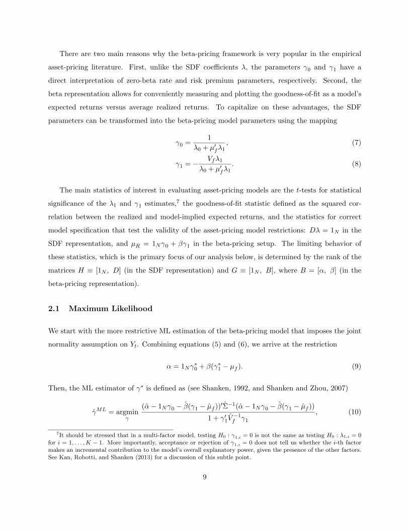
There are two main reasons why the beta-pricing framework is very popular in the empirical

asset-pricing literature. First, unlike the SDF coefficients λ, the parameters γ0 and γ1 have a

direct interpretation of zero-beta rate and risk premium parameters, respectively. Second, the

beta representation allows for conveniently measuring and plotting the goodness-of-fit as a model’s

expected returns versus average realized returns. To capitalize on these advantages, the SDF

parameters can be transformed into the beta-pricing model parameters using the mapping

γ0 =1

λ0 + µ′fλ1, (7)

γ1 = −Vfλ1

λ0 + µ′fλ1. (8)

The main statistics of interest in evaluating asset-pricing models are the t-tests for statistical

significance of the λ1 and γ1 estimates,7 the goodness-of-fit statistic defined as the squared cor-

relation between the realized and model-implied expected returns, and the statistics for correct

model specification that test the validity of the asset-pricing model restrictions: Dλ = 1N in the

SDF representation, and µR = 1Nγ0 + βγ1 in the beta-pricing setup. The limiting behavior of

these statistics, which is the primary focus of our analysis below, is determined by the rank of the

matrices H ≡ [1N , D] (in the SDF representation) and G ≡ [1N , B], where B = [α, β] (in the

beta-pricing representation).

2.1 Maximum Likelihood

We start with the more restrictive ML estimation of the beta-pricing model that imposes the joint

normality assumption on Yt. Combining equations (5) and (6), we arrive at the restriction

α = 1Nγ∗0 + β(γ∗1 − µf ). (9)

Then, the ML estimator of γ∗ is defined as (see Shanken, 1992, and Shanken and Zhou, 2007)

γML = argminγ

(α− 1Nγ0 − β(γ1 − µf ))′Σ−1(α− 1Nγ0 − β(γ1 − µf ))

1 + γ′1V−1f γ1

, (10)

7It should be stressed that in a multi-factor model, testing H0 : γ1,i = 0 is not the same as testing H0 : λ1,i = 0for i = 1, . . . ,K − 1. More importantly, acceptance or rejection of γ1,i = 0 does not tell us whether the i-th factormakes an incremental contribution to the model’s overall explanatory power, given the presence of the other factors.See Kan, Robotti, and Shanken (2013) for a discussion of this subtle point.

9

where α, β, µf , Vf , and Σ are the sample estimators of α, β, µf , Vf , and Σ, respectively. The test

for correct model specification of Shanken (1985) is given by

S = T minγ

(α− 1Nγ0 − β(γ1 − µf ))′Σ−1(α− 1Nγ0 − β(γ1 − µf ))

1 + γ′1V−1f γ1

, (11)

and is asymptotically distributed as S d→ χ2N−K under the null H0 : α = 1Nγ0 + β(γ1 − µf ).8

Due to the special structure of this objective function, the ML estimator of γ∗ can be obtained

explicitly as the solution to an eigenvector problem. Let v = [−γ0, 1, −(γ1 − µf )′]′ and G =

[1N , α, β], and noting that α − 1Nγ0 − β(γ1 − µf ) = Gv, we can write the objective function of

the ML estimator as

minv

v′G′Σ−1Gv

v′A(X ′X/T )−1A′v, (12)

where A = [0K , IK ]′ and X is a T × K matrix with a typical row x′t. Let v be the eigenvector

associated with the largest eigenvalue of9

Ω = (G′Σ−1G)−1[A(X ′X/T )−1A′]. (13)

Then, the ML estimator of γ∗ can be constructed as

γML0 = − v1

v2, (14)

γML1,i = µf,i −

vi+2

v2, i = 1, . . . ,K − 1. (15)

When the model is correctly specified and B is of full column rank, we have that Gv∗ = 0N for

v∗ = [−γ∗0, 1, −(γ∗1 − µf )′]′ and

√T

[γML0 − γ∗0γML1 − γ∗1

]d→ N

(0K , (1 + γ∗′1 V

−1f γ∗1)(B

′1Σ−1B1)

−1 +

[0 0′K−1

0K−1 Vf

]), (16)

where B1 = [1N , β]. As a result, the t-statistics for statistical significance of γ0 and γ1,i (i =

1, . . . ,K − 1) are constructed as

t(γML0 ) =

√T γML

0

s(γML0 )

, (17)

t(γML1,i ) =

√T γML

1,i

s(γML1,i )

, (18)

8Our limiting result for the S test is also applicable to the asymptotically equivalent likelihood ratio (LR) test,which is given by LR = T ln(1 + S/T ) (Shanken, 1985). Note also that in deriving the asymptotic distribution of S(and LR), the iid normality assumption can be relaxed to conditional normality of returns (conditional on ft). In fact,the asymptotic result for S (and LR) continues to hold under the more general case of conditional homoskedasticity.

9See also Zhou (1995) and Bekker, Dobbelstein, and Wansbeek (1996) for expressing the beta-pricing model as areduced rank regression whose parameters are obtained as an eigenvalue problem.

10

where s(γML0 ), s(γML

1,1 ), . . . , s(γML1,K−1) denote the square root of the diagonal elements of

(1 + γML′1 V −1f γML

1 )(B′1Σ−1B1)

−1 +

[0 0′K−1

0K−1 Vf

], (19)

and B1 = [1N , β]. Using the ML estimates γML0 and γML

1 , the ML estimate of β, βML

, and the

fitted expected returns on the test assets, µMLR , are obtained as

βML

= β +[α− 1N γ

ML0 − β(γML

1 − µf )]γML′1 V −1f

1 + γML′1 V −1f γML

1

(20)

and

µMLR = 1N γ

ML0 + β

MLγML1 . (21)

Since the empirical evidence strongly suggests that linear asset-pricing models are misspecified

(as emphasized in our empirical application and many papers in the literature), in the following

analysis we present results only for the misspecified model case.10 The following theorem (and

Auxiliary Lemma 1 in the Online Appendix) characterizes the limiting behavior of the ML estimates

γML, the t-statistics t(γML0 ) and t(γML

1,i ) (i = 1, . . . ,K − 1), and the pseudo-R2 statistic R2ML =

Corr(µMLR , µR)2 in misspecified models that contain a spurious factor.

Without loss of generality, we assume that the spurious factor is the last element of the vector

ft with βK−1 = 0N and is independent of the test asset returns and the other factors.11 Let Zi,

i = 0, . . . ,K − 2, denote a bounded random variable defined in the Online Appendix. Then, we

have the following result.

Theorem 1. Assume that Yt is iid normally distributed. Suppose that the model is misspecified

and it contains a spurious factor (that is, rank(B) = K − 1). Then, as T →∞, we have

(a) (i) t(γML0 )

d→ Z0; (ii) t(γML1,i )

d→ Zi for i = 1, . . . ,K − 2; and (iii) t2(γML1,K−1)

d→ χ2N−K+1;

(b) R2ML

p→ 1.

Proof. See the Online Appendix.

10The analytical and simulation results for the correctly specified model case are available from the authors uponrequest.

11Our analysis can be easily modified to deal with the case in which the betas of the factors are constant acrossassets instead of being equal to zero.

11

Theorem 1 establishes the limiting behavior of the t-tests, and pseudo-R2 statistic, R2ML, in

misspecified models with identification failure.12 The Online Appendix also shows that when a

spurious factor is present, the estimates on the useful factors are inconsistent and converge to

ratios of normal random variables while the estimate for the spurious factor (γML1,K−1) diverges

at rate root-T and the standardized estimator converges to the reciprocal of a normal random

variable.13 The t-tests for the useful factors converge to bounded random variables and, hence, are

inconsistent. In fact, as our simulations illustrate, the tests t(γML1,i ) for i = 1, . . . ,K − 2 tend to

exhibit power that is close to their size. In contrast, the t-test for the spurious factor will over-

reject substantially (with the probability of rejection rapidly approaching one as N increases) when

N (0, 1) critical values are used. Furthermore, part (b) of Theorem 1 shows that the pseudo-R2

of a misspecified model that contains a spurious factor approaches one. This leads to completely

spurious inference as the spurious factors do not contribute to the pricing performance of the model

and yet the sample pseudo-R2 would indicate that the model perfectly explains the cross-sectional

variations in the expected returns on the test assets.

Figure 5 about here

To visualize the limiting behavior of the t-statistics in part(a), Figure 5 plots the limiting

rejection rates of t(γML0 ), t(γML

1,i ), and t2(γML1,K−1) as functions of N−K when one uses the standard

normal critical values. The sample quantities that enter the computation for the t-statistics for

the constant term and the useful factor are calibrated to the CAPM model. Figure 5 confirms

that both t(γML0 ) and t(γML

1,i ) are inconsistent as their power does not go one. The over-rejection

(γML1,K−1) increases with N −K and is effectively one when N −K ≥ 15.

The full rank condition on G may also be violated when the model includes two (or more)

factors that are noisy versions of the same underlying factor. In this case (a proof for this result

is available from the authors upon request), the behavior of the parameter estimates, t-ratios, and

pseudo-R2 is the same as the one described in Theorem 1 with the limiting representations for the

12The t-statistics are constructed using a consistent estimator of the asymptotic variance for correctly specifiedmodels. For the form of the asymptotic variance of ML under misspecified models, see Gospodinov, Kan, and Robotti(2017a).

13Kan and Zhang (1999a) and Kleibergen (2009) also show that the estimate for the spurious factor diverges at rateroot-T when employing non-invariant two-pass cross-sectional regression estimators. Similar results are documentedby Kan and Zhang (1999b) and Gospodinov, Kan, and Robotti (2014) for models estimated via non-invariant (optimaland suboptimal) GMM.

12

noisy factors being the same as the asymptotic distribution for the spurious factor in part (a) of

Theorem 1.

2.2 Continuously-Updated GMM

We now consider the more general GMM estimation of SDF and beta-pricing models. We assume

that Yt is a jointly stationary and ergodic process with a finite fourth moment, and vec(Dt −D) is

a martingale difference sequence. The CU-GMM estimator of the SDF parameters λ∗ is defined as

(see Hansen, Heaton, and Yaron, 1996)

λ = argminλ

e(λ)′We(λ)−1e(λ), (22)

where e(λ) = T−1∑T

t=1 et(λ) and

We(λ) =1

T

T∑t=1

(et(λ)− e(λ))(et(λ)− e(λ))′. (23)

The over-identifying restriction test of the asset-pricing model is given by

J = T minλe(λ)′We(λ)−1e(λ), (24)

and J d→ χ2N−K when the asset-pricing model holds.

When the model is correctly specified and D is of full column rank, we have that (Hansen, 1982;

Newey and Smith, 2004)

√T (λ− λ∗) d→ N

(0K , (D

′We(λ∗)−1D)−1

), (25)

where We(λ∗) = E[et(λ

∗)et(λ∗)′]. The t-statistics for statistical significance of λ0 and λ1,i (i =

1, . . . ,K − 1) are constructed as

t(λ0) =

√T λ0

s(λ0), (26)

t(λ1,i) =

√T λ1,i

s(λ1,i), (27)

where the quantities s(λ0), s(λ1,1), . . . , s(λ1,K−1) denote the square root of the diagonal elements

of (D′We(λ)−1D)−1 and D is a consistent estimate of D. In the Online Appendix, we show that

13

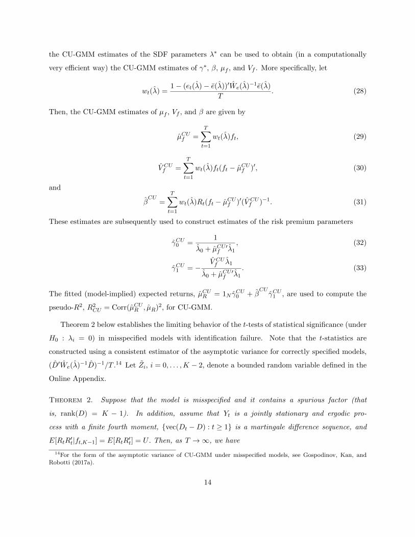
the CU-GMM estimates of the SDF parameters λ∗ can be used to obtain (in a computationally

very efficient way) the CU-GMM estimates of γ∗, β, µf , and Vf . More specifically, let

wt(λ) =1− (et(λ)− e(λ))′We(λ)−1e(λ)

T. (28)

Then, the CU-GMM estimates of µf , Vf , and β are given by

µCUf =T∑t=1

wt(λ)ft, (29)

V CUf =

T∑t=1

wt(λ)ft(ft − µCUf )′, (30)

and

βCU

=

T∑t=1

wt(λ)Rt(ft − µCUf )′(V CUf )−1. (31)

These estimates are subsequently used to construct estimates of the risk premium parameters

γCU0 =1

λ0 + µCU ′f λ1, (32)

γCU1 = −V CUf λ1

λ0 + µCU ′f λ1. (33)

The fitted (model-implied) expected returns, µCUR = 1N γCU0 + β

CUγCU1 , are used to compute the

pseudo-R2, R2CU = Corr(µCUR , µR)2, for CU-GMM.

Theorem 2 below establishes the limiting behavior of the t-tests of statistical significance (under

H0 : λi = 0) in misspecified models with identification failure. Note that the t-statistics are

constructed using a consistent estimator of the asymptotic variance for correctly specified models,

(D′We(λ)−1D)−1/T .14 Let Zi, i = 0, . . . ,K − 2, denote a bounded random variable defined in the

Online Appendix.

Theorem 2. Suppose that the model is misspecified and it contains a spurious factor (that

is, rank(D) = K − 1). In addition, assume that Yt is a jointly stationary and ergodic pro-

cess with a finite fourth moment, vec(Dt −D) : t ≥ 1 is a martingale difference sequence, and

E[RtR′t|ft,K−1] = E[RtR

′t] = U . Then, as T →∞, we have

14For the form of the asymptotic variance of CU-GMM under misspecified models, see Gospodinov, Kan, andRobotti (2017a).

14

(a) (i) t(λ0)d→ Z0 if µf,K−1 = 0 or t2(λ0)

d→ χ2N−K+1 if µf,K−1 6= 0; (ii) t(λ1,i)

d→ Zi for

i = 1, . . . ,K − 2; and (iii) t2(λ1,K−1)d→ χ2

N−K+1;

(b) R2CU

p→ 1.

Proof. See the Online Appendix.

Auxiliary Lemma 2 in the Online Appendix shows that when a spurious factor is present, the es-

timates on the useful factors (λ1,i (i = 1, . . . ,K−2)) converge to ratios of normal random variables.

The estimate for the spurious factor (λ1,K−1) diverges at rate root-T , and λ1,K−1/√T converges to

the reciprocal of a normal random variable.15 Based on Theorem 2, the t-tests of statistical signif-

icance for the useful factors converge to bounded random variables. As our simulations illustrate,

the tests t(λ1,i) for i = 1, . . . ,K−2 tend to exhibit power that is close to their size. In contrast, the

t-test for the spurious factor will overreject substantially (with the probability of rejection rapidly

approaching one as N increases) when N (0, 1) critical values are used. Another interesting feature

is that the asymptotic behavior of λ0 and t(λ0) changes in a discontinuous fashion depending on

whether the population mean of the spurious factor is zero or not. In the practically relevant case

of a nonzero mean, λ0 and t(λ0) inherit the limiting properties of λ1,K−1 and t(λ1,K−1) for the spu-

rious factor. Similarly to the beta-pricing setup, part (b) of Theorem 2 shows that the pseudo-R2

measure converges to one when one or more factors are spurious.

Figure 6 about here

The top graph in Figure 6 plots the limiting rejection rates of the t-statistics for a misspecified

model with a spurious factor. When the model is correctly specified, the limiting distribution for

the t-statistics for the useful factors is nonstandard but, unlike the misspecified model case, useful

factors that are priced are maintained in the model with probability approaching one. Although less

pronounced than in the misspecified model case, using N (0, 1) critical values will lead to substantial

overrejections of H0 : λ1,K−1 = 0 for the spurious factor. This is revealed by the bottom graph in

Figure 6.

15Kan and Zhang (1999a) and Kleibergen (2009) also show that the estimate for the spurious factor diverges at rateroot-T when employing non-invariant two-pass cross-sectional regression estimators. Similar results are documentedby Kan and Zhang (1999b) and Gospodinov, Kan, and Robotti (2014) for models estimated via non-invariant (optimaland suboptimal) GMM.

15

Figure 7 about here

The reason for the overrejection for the parameter on the spurious factor is clearly illustrated

in Figure 7 which plots the limiting probability density functions of t(λ1,K−1) under correctly

specified and misspecified models (N −K = 7), along with the standard normal density. Given the

bimodal shape and large variance of the probability density function of the limiting distribution

of t(λ1,K−1) under correctly specified models (which arises from the model’s underidentification),

using N (0, 1) critical values will lead to an overrejection of the hypothesis that the spurious factor

is not priced. This overrejection is further exacerbated by model misspecification, as illustrated

by the outward shift of the probability density function when the model is misspecified. Hence,

with lack of identification, misleading inference arises in correctly specified models as well as in

misspecified models, although the inference problems are more pronounced in the latter case.

3 Simulation Results

In this section, we undertake a Monte Carlo simulation experiment to study the empirical rejection

rates of the t-tests for the CU-GMM and ML estimators as well as the finite-sample distribution

of the goodness-of-fit measure. We consider three linear models: (i) a model with a constant term

and a useful factor, (ii) a model with a constant term and a spurious factor, and (iii) a model with

a constant term, a useful, and a spurious factor. All three models are misspecified.

The returns on the test assets and the useful factor are drawn from a multivariate normal

distribution. In all simulation designs, the covariance matrix of the simulated test asset returns

is set equal to the sample covariance matrix from the 1967:1–2012:12 sample of monthly gross

returns on the 25 Fama-French size and book-to-market ranked portfolios (from Kenneth French’s

website). The means of the simulated returns are set equal to the sample means of the actual

returns, and they are not exactly linear in the chosen betas for the useful factors. As a result, the

models are misspecified in all three cases. The mean and variance of the simulated useful factor

are calibrated to the sample mean and variance of the value-weighted market excess return. The

covariances between the useful factor and the returns are chosen based on the sample covariances

estimated from the data. The spurious factor is generated as a standard normal random variable

which is independent of the returns and the useful factor. The time series sample size is T = 200,

16

600, and 1000, and all results are based on 100,000 Monte Carlo replications. We also report the

limiting rejection probabilities (denoted by T =∞) for the t-tests based on our asymptotic results

in Section 2.

Table 3 about here

A popular way to look at the performance of the model is to compute the squared correlation

between the expected fitted returns of the model and the average realized returns. The distribution

of this pseudo-R2 is reported in Table 3. Again, as our theoretical analysis suggests, the empirical

distribution of the pseudo-R2 in models with a spurious factor collapses to 1 as the sample size

gets large. For example, this measure will indicate a perfect fit for models that include a factor

that is independent of the returns on the test assets. These spurious results should serve as a

warning signal in applied work where many macroeconomic factors are only weakly correlated with

the returns on the test assets.

Table 4 about here

Table 4 presents the rejection probabilities of the t-tests of H0 : λ1,i = 0 and H0 : γ1,i =

0 (tests of statistical significance) for the useful and the spurious factor in the SDF and beta

representations of models (i), (ii), and (iii). The t-statistics are computed under the assumption

that the model is correctly specified and are compared against the critical values from the standard

normal distribution, as is commonly done in the literature. Table 4 reveals that for models with

a spurious factor, the t-tests will give rise to spurious results, suggesting that these completely

irrelevant factors are priced. Moreover, the spurious factor (which, by construction, does not

contribute to the pricing performance of the model) drives out the useful factor and leads to the

grossly misleading conclusion to keep the spurious factor and drop the useful factor from the model

(see Panel C of Table 4).

The lack of power of the specification tests, the spuriously high pseudo-R2 values, and the perils

of relying on the traditional t-tests of parameter significance in unidentified models suggest that

the decision regarding the model specification should be augmented with additional diagnostics.

One approach to restoring the validity of the standard inference is based on the following model

17

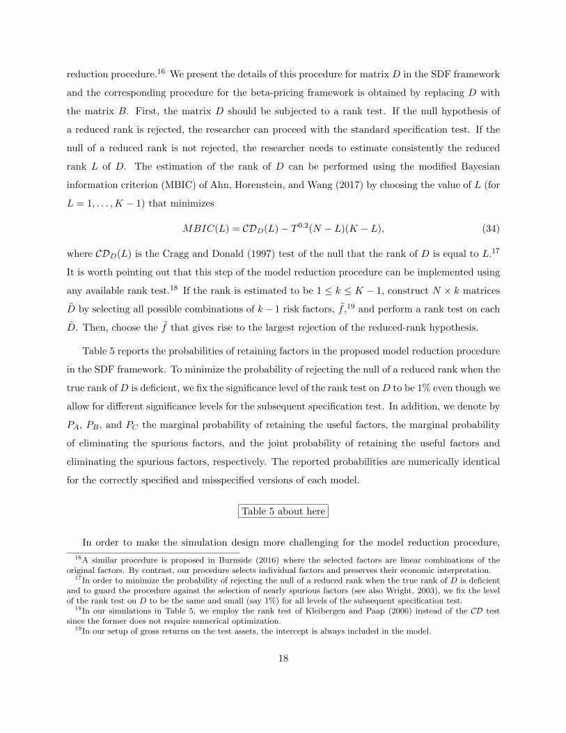
reduction procedure.16 We present the details of this procedure for matrix D in the SDF framework

and the corresponding procedure for the beta-pricing framework is obtained by replacing D with

the matrix B. First, the matrix D should be subjected to a rank test. If the null hypothesis of

a reduced rank is rejected, the researcher can proceed with the standard specification test. If the

null of a reduced rank is not rejected, the researcher needs to estimate consistently the reduced

rank L of D. The estimation of the rank of D can be performed using the modified Bayesian

information criterion (MBIC) of Ahn, Horenstein, and Wang (2017) by choosing the value of L (for

L = 1, . . . ,K − 1) that minimizes

MBIC(L) = CDD(L)− T 0.2(N − L)(K − L), (34)

where CDD(L) is the Cragg and Donald (1997) test of the null that the rank of D is equal to L.17

It is worth pointing out that this step of the model reduction procedure can be implemented using

any available rank test.18 If the rank is estimated to be 1 ≤ k ≤ K − 1, construct N × k matrices

D by selecting all possible combinations of k− 1 risk factors, f ,19 and perform a rank test on each

D. Then, choose the f that gives rise to the largest rejection of the reduced-rank hypothesis.

Table 5 reports the probabilities of retaining factors in the proposed model reduction procedure

in the SDF framework. To minimize the probability of rejecting the null of a reduced rank when the

true rank of D is deficient, we fix the significance level of the rank test on D to be 1% even though we

allow for different significance levels for the subsequent specification test. In addition, we denote by

PA, PB, and PC the marginal probability of retaining the useful factors, the marginal probability

of eliminating the spurious factors, and the joint probability of retaining the useful factors and

eliminating the spurious factors, respectively. The reported probabilities are numerically identical

for the correctly specified and misspecified versions of each model.

Table 5 about here

In order to make the simulation design more challenging for the model reduction procedure,

16A similar procedure is proposed in Burnside (2016) where the selected factors are linear combinations of theoriginal factors. By contrast, our procedure selects individual factors and preserves their economic interpretation.

17In order to minimize the probability of rejecting the null of a reduced rank when the true rank of D is deficientand to guard the procedure against the selection of nearly spurious factors (see also Wright, 2003), we fix the levelof the rank test on D to be the same and small (say 1%) for all levels of the subsequent specification test.

18In our simulations in Table 5, we employ the rank test of Kleibergen and Paap (2006) instead of the CD testsince the former does not require numerical optimization.

19In our setup of gross returns on the test assets, the intercept is always included in the model.

18

we also consider, in addition to the three models described above, a model with a constant term,

three useful, and two spurious factors. The results for all models suggest that our model selection

procedure is very effective in retaining the useful factors and eliminating the spurious factors from

the analysis. For sample sizes T ≥ 600, the most challenging scenario of a model with three useful

and two spurious factors retains (removes) the useful (spurious) factors with probability one.

4 Empirical Illustration

We evaluate the performance of several prominent asset-pricing models with traded and non-traded

factors in light of our analytical and simulation results in Sections 2 and 3. First, we describe the

data used in the empirical analysis and outline the different specifications of the asset-pricing models

considered. Next, we present our results.

4.1 Data and Asset-Pricing Models

The return data are from Kenneth French’s website and consist of the monthly value-weighted gross

returns on the (i) 25 Fama-French size and book-to-market ranked portfolios, (ii) 25 Fama-French

size and momentum ranked portfolios, and (iii) 32 Fama-French size, operating profitability, and

investment ranked portfolios. To conserve space, we briefly summarize the results for other sets of

test portfolio returns at the end of the section. The data are from January 1967 to December 2012

(552 monthly observations). The beginning date of our sample period is dictated by profitability and

investment data availability.20 We analyze six asset-pricing models starting with the conditional

labor model (C-LAB) of Jagannathan and Wang (1996). This model incorporates measures of

the return on human capital as well as the change in financial wealth and allows the conditional

moments to vary with a state variable, prem, the lagged yield spread between Baa- and Aaa-rated

corporate bonds from the Board of Governors of the Federal Reserve System. The SDF specification

for this model is

yC−LABt = λ0 + λvw vwt + λlabor labort + λprem premt, (35)

where vw is the excess return (in excess of the 1-month T-bill rate from Ibbotson Associates) on

the value-weighted stock market index (NYSE-AMEX-NASDAQ) from Kenneth French’s website,

20We thank Lu Zhang for sharing his data with us.

19

labor is the growth rate in per capita labor income, L, defined as the difference between total

personal income and dividend payments, divided by the total population (from the Bureau of

Economic Analysis). Following Jagannathan and Wang (1996), we use a 2-month moving average

to construct the growth rate labort = (Lt−1+Lt−2)/(Lt−2+Lt−3)−1, for the purpose of minimizing

the influence of measurement error. The corresponding cross-sectional specification is µR = 1Nγ0+

βvwγvw + βlaborγlabor + βpremγprem.

Our second model (CC-CAY) is a conditional version of the consumption CAPM due to Lettau

and Ludvigson (2001) with

yCC−CAYt = λ0 + λcg cgt + λcay cayt−1 + λcg·cay cgt · cayt−1, (36)

where cg is the growth rate in real per capita nondurable consumption (seasonally adjusted at

annual rates) from the Bureau of Economic Analysis, and cay, the conditioning variable, is a

consumption-aggregate wealth ratio.21 This specification is obtained by scaling the constant term

and the cg factor of a linearized consumption CAPM by a constant and cay. The beta-pricing

specification is µR = 1Nγ0 + βcgγcg + βcayγcay + βcg·cayγcg·cay.

The third model (ICAPM) is an empirical implementation of Merton’s (1973) intertemporal

extension of the CAPM based on Campbell (1996), who argues that innovations in state variables

that forecast future investment opportunities should serve as the factors. The candidate SDF for

the five-factor specification proposed by Petkova (2006) is

yICAPMt = λ0 + λvw vwt + λterm termt + λdef deft + λdiv divt + λrf rft, (37)

where term is the difference between the yields of 10- and 1-year government bonds (from the

Board of Governors of the Federal Reserve System), def is the difference between the yields of

long-term corporate Baa bonds and long-term government bonds (from Ibbotson Associates), div

is the dividend yield on the Center for Research in Security Prices (CRSP) value-weighted stock

market portfolio, and rf is the 1-month T-bill yield (from CRSP, Fama Risk Free Rates). The

actual factors for term, def , div, and rf are their innovations from a VAR(1) system of seven

state variables that also includes vw, smb, and hml (the market, size, and value factors of the

three-factor model of Fama and French, 1993). As for the beta-pricing specification, we have

µR = 1Nγ0 + βvwγvw + βtermγterm + βdefγdef + βdivγdiv + βrfγrf .

21Following Vissing-Jørgensen and Attanasio (2003), we linearly interpolate the quarterly values of cay to permitanalysis at the monthly frequency.

20

We complete our list of models with traded and non-traded factors by considering a specification

(D-CCAPM), due to Yogo (2006), which highlights the cyclical role of durable consumption in asset

pricing. The candidate SDF is given by

yD−CCAPMt = λ0 + λvw vwt + λcg cgt + λcgdur cgdurt, (38)

where cgdur is the growth rate in real per capita durable consumption (seasonally adjusted at

annual rates) from the Bureau of Economic Analysis. In beta form, we have µR = 1Nγ0+βvwγvw+

βcgγcg + βcgdurγcgdur.

Our fifth model (FF3), due to Fama and French (1993),

yFF3t = λ0 + λvw vwt + λsmb smbt + λhml hmlt, (39)

includes two empirically motivated factors, smb, the return difference between portfolios of stocks

with small and large market capitalizations, and hml, the return difference between portfolios of

stocks with high and low book-to-market ratios (from Kenneth French’s website). The familiar

beta representation of the model is µR = 1Nγ0 + βvwγvw + βsmbγsmb + βhmlγhml.

Finally, we consider a newly proposed empirical specification (HXZ), due to Hou, Xue, and

Zhang (2015), which is built on the neoclassical q-theory of investment. The candidate SDF for

this model is

yHXZt = λ0 + λvw vwt + λme met + λroe roet + λia iat, (40)

where me is the difference between the return on a portfolio of small size stocks and the return on a

portfolio of big size stocks, roe is the difference between the return on a portfolio of high profitability

stocks and the return on a portfolio of low profitability stocks, and ia is the difference between the

return on a portfolio of low investment stocks and the return on a portfolio of high investment stocks.

This four-factor model has been shown to successfully explain many asset-pricing anomalies.22 The

corresponding beta representation of the model is µR = 1Nγ0+βvwγvw+βmeγme+βroeγroe+βiaγia.

22Empirical results for the five-factor model of Fama and French (2015), the three-factor model of Fama and French(1993) augmented with the momentum factor of Carhart (1997), and the three-factor model of Fama and French(1993) augmented with the non-traded liquidity factor of Pastor and Stambaugh (2003) are available from the authorsupon request.

21

4.2 Results

Starting with C-LAB, we investigate whether this model is well identified. To this end, we employ

the rank test of Cragg and Donald (1997) and consider two test statistics, CDSDF in the SDF setup

and CDBeta in the beta setup. To understand how CDSDF and CDBeta are computed, let Π be an

N ×K matrix and denote its estimate by Π. Assume that√Tvec(Π−Π)

d→ N (0NK ,M), where M

is a finite and positive-definite matrix. Under the null that Π is of (reduced) column rank K − 1,

H0 : rank(Π) = K−1, there exists a nonzero K-vector c such that Πc = 0N with the normalization

c′c = 1. The Cragg and Donald (1997) test of H0 : rank(Π) = K − 1 takes the form

CD = minc:c′c=1

c′Π′[c′ ⊗ IN )M(c⊗ IN )]−1Πc, (41)

where Π and M are consistent estimates of Π and M , respectively.

In the SDF framework, we have Π = D and M = 1T

∑Tt=1 vec(Dt − D)vec(Dt − D)′. We de-

note this rank test by CDSDF . In the beta-pricing model setup, we have Π = B = [α, β] and

M =

[(T−1

∑Tt=1 xtx

′t

)−1⊗ IN

] [T−1

∑Tt=1(xtx

′t)⊗ (ete

′t)] [(

T−1∑T

t=1 xtx′t

)−1⊗ IN

], where

et = Rt− Bxt. The corresponding rank test in the beta-pricing framework is denoted by CDBeta.23

Table 6 about here

The outcomes of the two rank tests suggest that C-LAB is poorly identified across different sets

of test assets. The p-values of these tests are large, ranging from 0.55 to 0.82 in the SDF setup

and from 0.34 to 0.74 in the beta setup, and indicate that the null hypothesis of a deficient column

rank for the D and B matrices cannot be rejected. Consistent with our analytical results, this

identification failure results in the inability of the J and S specification tests to reject the models

and in spuriously high pseudo-R2s for CU-GMM and ML. Across panels, the pseudo-R2 values for

C-LAB (see the columns labeled “all” in the table) range from 0.98 to 0.99 for CU-GMM and are

indistinguishable from 1 for ML. Based on J , S, and the CU-GMM and ML pseudo-R2s, C-LAB

appears to have a spectacular fit and a researcher would likely proceed with t-tests of parameter

significance with standard errors computed under the assumption of correct model specification.

This would lead us to conclude that the labor and prem factors are often priced in the cross-section

23In the model selection procedure described below, we employ this heteroskedasticity-robust version of the CDtest for both ML and CSR GLS even though the ML estimation imposes homoskedasticity on the data.

22

of expected returns, as emphasized by the high traditional t-ratios on the prem and labor factors for

CU-GMM and ML. Interestingly, the evidence of pricing for the market factor is rather weak, with

traditional absolute t-ratio values ranging from 1.29 to 1.73 for CU-GMM and from 0.67 to 1.42 for

ML. These empirical findings are again consistent with our methodological findings and reveal the

spurious nature of inference as factors that are spurious are selected with high probability, while

factors that are useful (such as the market factor) are driven out of the model.

Applying the model reduction procedure, described in Section 3, to C-LAB reveals that only

the market factor survives the selection procedure. Essentially, C-LAB reduces to CAPM and the

J and S tests now have power to reject the model (see columns labeled “selected” in the table). In

turn, the pseudo R2s provide a completely different and more realistic assessment of the goodness-

of-fit of the model, ranging from 0.23 to 0.54 for CU-GMM and from 0.11 to 0.14 for ML. The high

misspecification-robust t-ratios on vw in Panel A suggest some strong pricing ability for the market

factor when portfolios are formed on size and book-to-market.24 In contrast, when considering

portfolios formed on size and momentum, the evidence of pricing for vw is very limited, consistent

with the uncontroversial finding that CAPM cannot explain the returns on portfolios formed on

momentum. Panel C also shows that the pricing ability of vw is rather weak when employing

misspecification-robust t-ratios and considering portfolios formed on size, operating profitability,

and investment.

It should be noted that non-invariant estimators, such as the HJ-distance and CSR GLS esti-

mators, provide a less optimistic picture of C-LAB compared to CU-GMM and ML. The p-values

of HJD and GLS in Table 6 are always zero even before applying the model selection procedure just

described. Therefore, even if HJD and GLS are inconsistent under identification failure (a proof

of this claim is available from the authors upon request), they seem to be more robust to lack of

identification and can detect model misspecification with higher probability than their invariant

counterparts. In sharp contrast with the pseudo-R2s for CU-GMM and ML, the pseudo-R2s for

the non-invariant estimators are relatively small and range from 0.03 to 0.66 for HJ-distance and

from 0.07 to 0.69 for GLS CSR (see the columns labeled “all” in the table). Finally, after applying

our model selection procedure, the pricing implications for vw (based on misspecification-robust

24See Gospodinov, Kan, and Robotti (2017a) for the derivation of misspecification-robust t-ratios for CU-GMMand ML.

23

t-ratios) are largely consistent across invariant and non-invariant estimators.25

The spurious nature of the results analyzed in this paper are probably best illustrated with

CC-CAY in Table 7.

Table 7 about here

The rank tests in all three panels provide strong evidence that the models are unidentified.

Ignoring the outcome of the rank tests would lead us to conclude that the models estimated by

CU-GMM and ML are correctly specified and that scaled consumption growth, cg · cay, is highly

significant. However, none of the factors survive after applying the proposed model selection pro-

cedure since none of the factors (or a subset of factors) in this model satisfy the rank condition.

Tables 8 and 9 about here

The results for ICAPM and D-CCAPM in Tables 8 and 9 further reveal the fragility of statistical

inference in models with factors that are only weakly correlated with the test asset returns. As for

C-LAB in Table 6, only the market factor survives the selection procedure in D-CCAPM. While the

factors div and rf are selected for some test assets in the final specification of ICAPM in Table 8,

their t-statistics are all insignificant when constructed using misspecification-robust standard errors.

Tables 10 and 11 about here

Turning to models with traded factors only, the results for the rank tests in Tables 10 and 11

for FF3 and HXZ suggest that these models are well-identified at the 5% significance level, albeit

misspecified (except for the CU-GMM estimator in Panel C of Table 11). We should note that even

for models with traded factors, the inference based on non-invariant (HJ-distance and GLS CSR)

estimators appears to be more stable and reliable than the inference based on invariant (CU-GMM

and ML) estimators.

Overall, our empirical analysis reveals that, for models with non-traded factors, both the SDF

and beta-pricing setups are affected by the weak identification problem and share similar pricing

25The misspecification-robust t-ratios for HJ-distance are provided in Kan and Robotti (2009), while the ones forGLS CSR can be found in Kan, Robotti, and Shanken (2013).

24

implications once our model selection procedure and misspecification-robust standard errors are

used. It should also be noted that the ML results are based on the joint normality assumption

on the factors and the returns. This assumption could be relaxed by adopting a quasi-maximum

likelihood framework as, for example, in White (1994). Alternatively, a researcher could use CU-

GMM to estimate the parameters of the asset-pricing model in beta-pricing form as described in

the Online Appendix.

Finally, in unreported empirical investigations, we explored the performance of these six models

using the (i) 25 Fama-French portfolios formed on size and short-term reversal, (ii) 25 Fama-French

portfolios formed on size and long-term reversal, and (iii) 25 Fama-French portfolios formed on

size and book-to-market plus 17 industry portfolios (all the test assets are from Kenneth French’s

website). The results based on these three additional sets of test asset returns are largely consistent

with the results reported in the paper. However, at least in the SDF formulation of the model, the

identification issues become more severe when using the 25 Fama-French portfolios formed on size

and short-term reversal and the 25 Fama-French portfolios formed on size and long-term reversal,

consistent with the relatively uncontroversial finding in the literature that all these models have

problems in explaining short- and long-term reversal. In these latter cases, even models with traded

factors only, such as FF3 and HXZ, start to exhibit some non-trivial patterns of weak identification.

Our main empirical findings can be summarized as follows. Models with non-traded factors

are often poorly identified, and tend to produce highly misleading inference in terms of spuriously

high statistical significance and lack of power in rejecting the null of correct model specification.

In addition to the outcome of the rank tests, two observations cast doubts on the validity of the

results for these models: (i) the difference between the t-statistics computed under the assumption

of correct specification and the misspecification-robust t-statistics (with the misspecification-robust

t-statistics being typically statistically insignificant), and (ii) the unrealistically high value of the

pseudo-R2. The models that perform the best are FF3 and especially HXZ where all the factors

appear to contribute to pricing and are characterized by statistically significant risk premia. Out

of the different sets of test portfolios, the portfolios formed on size and momentum, size and short-

and long-term reversal appear to be the most challenging from a pricing perspective.

25

5 Concluding Remarks

In this paper, we study the limiting properties of some invariant tests of asset-pricing models, and

show that the inference based on these tests can be spurious when the models are unidentified.

The spurious results in these models arise from the combined effect of identification failure and

model misspecification. It is important to stress that this is not an isolated problem limited to a

particular sample (data frequency), test assets, and asset-pricing models. This suggests that the

statistical evidence on the pricing ability of many macro factors and their usefulness in explaining

the cross-section of asset returns should be interpreted with caution. Some warning signs about

this problem (for example, the outcome of a rank test) are often ignored by applied researchers.

While non-invariant estimators (HJ-distance non-optimal GMM and GLS two-pass cross-sectional

regressions) also suffer from similar problems, the invariant (CU-GMM and ML) estimators turn

out to be much more sensitive to model misspecification and lack of identification.

Given the severity of the inference problems associated with invariant estimators of possibly

unidentified and misspecified asset-pricing models that we document in this paper, our recommen-

dations for empirical practice can be summarized as follows. Importantly, any model should be

subjected to a rank test which will provide evidence on whether the model parameters are identified

or not. If the null hypothesis of a reduced rank is rejected, the researcher can proceed with the

standard tools for inference in analyzing and evaluating the model. If the null of a reduced rank is

not rejected, the researcher needs to estimate consistently the reduced rank of the model and select

the combination of factors that delivers the largest rejection of the reduced rank hypothesis. This

procedure would restore the standard inference although it may still need to be robustified against

possible model misspecification as in Gospodinov, Kan, and Robotti (2017a). An alternative em-

pirical strategy is to work with non-invariant estimators (HJ-distance and cross-sectional regression

estimators) and pursue misspecification-robust inference that is asymptotically valid regardless of

the degree of identification (see Gospodinov, Kan, and Robotti, 2014).26

26See also Bryzgalova (2016) and Feng, Giglio, and Xiu (2017) for newly proposed model-selection methods basedon the lasso estimator in a two-pass setting.

26

References

[1] Ahn, Seung C., Alex R. Horenstein, and Na Wang, 2017, Beta matrix and common factors in

stock returns, Journal of Financial and Quantitative Analysis, forthcoming.

[2] Almeida, Caio, and Rene Garcia, 2012, Assessing misspecified asset pricing models with em-

pirical likelihood estimators, Journal of Econometrics 170, 519–537.

[3] Almeida, Caio, and Rene Garcia, 2017, Economic implications of nonlinear pricing kernels,

Management Science, forthcoming.

[4] Barillas, Francisco, and Jay Shanken, 2017a, Which alpha?, Review of Financial Studies 30,

1316–1338.

[5] Barillas, Francisco, and Jay Shanken, 2017b, Comparing asset pricing models, Journal of

Finance, forthcoming.

[6] Bekker, Paul, Pascal Dobbelstein, and Tom Wansbeek, 1996, The APT model as reduced-rank

regression, Journal of Business and Economic Statistics 14, 199–202.

[7] Bryzgalova, Svetlana, 2016, Spurious factors in linear asset pricing models, Working Paper.

[8] Burnside, Craig, 2016, Identification and inference in linear stochastic discount factor models

with excess returns, Journal of Financial Econometrics 14, 295–330.

[9] Campbell, John Y., 1996, Understanding risk and return, Journal of Political Economy 104,

298–345.

[10] Carhart, Mark M., 1997, On persistence in mutual fund performance, Journal of Finance 52,

57–82.

[11] Cragg, John G., and Stephen G. Donald, 1997, Inferring the rank of a matrix, Journal of

Econometrics 76, 223–250.

[12] Fama, Eugene F., and Kenneth R. French, 1993, Common risk factors in the returns on stocks

and bonds, Journal of Financial Economics 33, 3–56.

[13] Fama, Eugene F., and Kenneth R. French, 2015, A five-factor asset pricing model, Journal of

Financial Economics 116, 1–22.

27

[14] Feng, Guanhao, Stefano Giglio, and Dacheng Xiu, 2017, Taming the factor zoo, Chicago Booth

Research Paper No. 17-04.

[15] Ghosh, Anisha, Christian Julliard, and Alex P. Taylor, 2017, What is the consumption-CAPM

missing? An information-theoretic framework for the analysis of asset pricing models, Review

of Financial Studies 30, 442–504.

[16] Gospodinov, Nikolay, Raymond Kan, and Cesare Robotti, 2014, Misspecification-robust infer-

ence in linear asset-pricing models with irrelevant risk factors, Review of Financial Studies 27,

2139–2170.

[17] Gospodinov, Nikolay, Raymond Kan, and Cesare Robotti, 2017a, Asymptotic variance ap-

proximations for invariant estimators in uncertain asset-pricing models, Econometric Reviews,

forthcoming.

[18] Gospodinov, Nikolay, Raymond Kan, and Cesare Robotti, 2017b, Spurious Inference in

reduced-rank asset-pricing models, Econometrica 85, 1613–1628.

[19] Granger, Clive W. J., and Paul Newbold, 1974, Spurious regressions in econometrics, Journal

of Econometrics 2, 111–120.

[20] Hall, Alastair R., 2005, Generalized Method of Moments. Oxford University Press, Oxford.

[21] Hansen, Lars P., 1982, Large sample properties of generalized method of moments estimators,

Econometrica 50, 1029–1054.

[22] Hansen, Lars P., John Heaton, and Amir Yaron, 1996, Finite-sample properties of some alter-

native GMM estimators, Journal of Business and Economic Statistics 14, 262–280.

[23] Hansen, Lars P., and Ravi Jagannathan, 1997, Assessing specification errors in stochastic

discount factor models, Journal of Finance 52, 557–590.

[24] Harvey, Campbell R., Yan Liu, and Heqing Zhu, 2016, . . . and the cross-section of expected

returns, Review of Financial Studies 29, 5–68.

[25] Hou, Kewei, Chen Xue, and Lu Zhang, 2015, Digesting anomalies: An investment approach,

Review of Financial Studies 28, 650–705.

28

[26] Jagannathan, Ravi, and Zhenyu Wang, 1996, The conditional CAPM and the cross-section of

expected returns, Journal of Finance 51, 3–53.

[27] Kan, Raymond, and Cesare Robotti, 2009, Model comparison using the Hansen-Jagannathan

distance, Review of Financial Studies 22, 3449–3490.

[28] Kan, Raymond, Cesare Robotti, and Jay Shanken, 2013, Pricing model performance and the

two-pass cross-sectional regression methodology, Journal of Finance 68, 2617–2649.

[29] Kan, Raymond and Chu Zhang, 1999a, Two-pass tests of asset pricing models with useless

factors, Journal of Finance 54, 203–235.

[30] Kan, Raymond, and Chu Zhang, 1999b, GMM tests of stochastic discount factor models with

useless factors, Journal of Financial Economics 54, 103–127.

[31] Kleibergen, Frank, 2009, Tests of risk premia in linear factor models, Journal of Econometrics

149, 149–173.

[32] Kleibergen, Frank, and Richard Paap, 2006, Generalized reduced rank tests using the singular

value decomposition, Journal of Econometrics 133, 97–126.

[33] Kleibergen, Frank, and Zhaoguo Zhan, 2015, Unexplained factors and their effects on second

pass R-squared’s, Journal of Econometrics 189, 101–116.

[34] Lettau, Martin, and Sydney C. Ludvigson, 2001, Resurrecting the (C)CAPM: A cross-sectional

test when risk premia are time-varying, Journal of Political Economy 109, 1238–1287.

[35] Lewellen, Jonathan W., Stefan Nagel, and Jay Shanken, 2010, A skeptical appraisal of asset-

pricing tests, Journal of Financial Economics 96, 175–194.

[36] Manresa, Elena, Francisco Penaranda, and Enrique Sentana, 2017, Empirical evaluation of

overspecified asset pricing models, CEPR Discussion Paper No. DP12085.

[37] Merton, Robert C., 1973, An intertemporal capital asset pricing model, Econometrica 41,

867–887.

[38] Newey, Whitney K., and Richard J. Smith, 2004, Higher order properties of GMM and gener-

alized empirical likelihood estimators, Econometrica 72, 219–255.

29

[39] Pastor, Lubos, and Robert F. Stambaugh, 2003, Liquidity risk and expected stock returns,

Journal of Political Economy 111, 642–685.

[40] Penaranda, Francisco, and Enrique Sentana, 2015, A unifying approach to the empirical eval-

uation of asset pricing models, Review of Economics and Statistics 97, 412–435.

[41] Petkova, Ralitsa, 2006, Do the Fama-French factors proxy for innovations in predictive vari-

ables?, Journal of Finance 61, 581–612.

[42] Phillips, Peter C. B., 1989, Partially identified econometric models, Econometric Theory 5,

181–240.

[43] Shanken, Jay, 1985, Multivariate tests of the zero-beta CAPM, Journal of Financial Economics

14, 327–348.

[44] Shanken, Jay, 1992, On the estimation of beta-pricing models, Review of Financial Studies 5,

1–33.

[45] Shanken, Jay, and Guofu Zhou, 2007, Estimating and testing beta pricing models: Alternative

methods and their performance in simulations, Journal of Financial Economics 84, 40–86.

[46] Vissing-Jørgensen, Annette, and Orazio P. Attanasio, 2003, Stock-market participation, in-

tertemporal substitution, and risk-aversion, American Economic Review Papers and Proceed-

ings 93, 383–391.

[47] White, Halbert L., 1994, Estimation, Inference and Specification Analysis. Cambridge Univer-

sity Press, New York.

[48] Wright, Jonathan H., 2003, Detecting lack of identification in GMM, Econometric Theory 19,

322–330.

[49] Yogo, Motohiro, 2006, A consumption-based explanation of expected stock returns, Journal

of Finance 61, 539–580.

[50] Zhou, Guofu, 1995, Small sample rank tests with applications to asset pricing, Journal of

Empirical Finance 2, 71–93.

30

Table 1Test Statistics for CAPM and CAPM Augmented with the “sp” Factor

The table reports test statistics for the CAPM, the CAPM augmented with the “sp” factor, and a model withthe “sp” factor only. J denotes Hansen, Heaton, and Yaron’s (1996) test for over-identifying restrictionsbased on the CU-GMM estimator. S denotes Shanken’s (1985) Wald-type test of correct model specificationbased on the ML estimator. tx denotes the t-test of statistical significance for the parameter associatedwith factor x, with standard errors computed under the assumption of correct model specification. Finally,R2 denotes the squared correlation coefficient between the fitted expected returns and the average realizedreturns.

Panel A: CU-GMM

CAPM CAPM + “sp” factor “sp” factor

tvw(p-value)

5.28(0.0000)

0.85(0.3954)

tsp(p-value)

5.08(0.0000)

5.12(0.0000)

J(p-value)

62.20(0.0000)

25.53(0.2726)

25.96(0.3029)

R2 0.2277 0.9928 0.9938

Panel B: ML

CAPM CAPM + “sp” factor “sp” factor

tvw(p-value)

−3.65(0.0003)

0.52(0.6027)

tsp(p-value)

−4.62(0.0000)

−4.64(0.0000)

S(p-value)

68.79(0.0000)

21.32(0.5011)

21.56(0.5471)

R2 0.1447 0.9999 1.0000

31

Table 2Test Statistics for Various Asset-Pricing Models

The table reports test statistics for four asset-pricing models: CAPM, FF3, C-LAB, and CC-CAY. CDSDF

and CDBeta denote the Cragg and Donald (1997) test for the null of a reduced rank in the SDF and beta-pricing setups, respectively. HJD and GLS denote the tests of correct model specification based on thedistance measure of Hansen and Jagannathan (1997) and on the generalized least squares cross-sectionalregression test of Shanken (1985). J denotes Hansen, Heaton, and Yaron’s (1996) test for over-identifyingrestrictions based on the CU-GMM estimator. S denotes Shanken’s (1985) Wald-type test of correct modelspecification based on the ML estimator. The rows for the different factors report the t-tests of statisticalsignificance with standard errors computed under the assumption of correct model specification. Finally,R2 denotes the squared correlation coefficient between the fitted expected returns and the average realizedreturns.

Panel A: Rank, HJD, and GLS Tests

CAPM FF3 C-LAB CC-CAY

CDSDF(p-value)

157.03(0.0000)

109.73(0.0000)

18.72(0.6626)

12.34(0.9499)

HJD(p-value)

69.35(0.0000)

53.48(0.0005)

67.24(0.0000)

70.15(0.0009)

CDBeta(p-value)

493.38(0.0000)

298.24(0.0000)

24.09(0.3427)

15.16(0.8552)

GLS(p-value)

71.96(0.0000)

55.61(0.0004)

69.68(0.0000)

71.77(0.0009)

Panel B: CU-GMM

CAPM FF3 C-LAB CC-CAY

J(p-value)

62.20(0.0000)

44.26(0.0022)

18.01(0.6487)

12.46(0.9264)

vw 5.28 4.78 1.73smb −4.60hml −2.93labor 0.17prem −4.16cg 2.85cay 1.79cg · cay −3.17R2 0.2277 0.7783 0.9788 0.9457

Panel C: ML

CAPM FF3 C-LAB CC-CAY

S(p-value)

68.79(0.0000)

51.05(0.0003)

20.87(0.4672)

13.85(0.8758)

vw −3.65 −3.80 1.42smb 1.73hml 3.04labor −3.14prem −4.07cg −2.23cay −0.77cg · cay 3.63R2 0.1447 0.7337 1.0000 0.9995

32

Table 3Empirical Distribution of the R2 Coefficient

The table presents the empirical distribution of the pseudo-R2 computed as the squared correlation betweenthe realized and fitted expected returns based on the CU-GMM and ML estimators, respectively. Theresults are based on 100,000 simulations, assuming that the returns are generated from a multivariate normaldistribution with means and covariance matrix calibrated to the 25 size and book-to-market Fama-Frenchportfolio returns for the period 1967:1–2012:12.

T mean std 1% 5% 10% 25% 50% 75% 90% 95% 99%

Panel A: Model with a Useful Factor Only

CU-GMM200 0.304 0.249 0.000 0.003 0.013 0.076 0.257 0.496 0.678 0.759 0.868600 0.235 0.185 0.000 0.004 0.015 0.074 0.202 0.364 0.506 0.582 0.7021000 0.217 0.156 0.000 0.009 0.027 0.089 0.195 0.322 0.438 0.506 0.617

ML200 0.234 0.222 0.000 0.002 0.006 0.041 0.165 0.383 0.582 0.677 0.808600 0.186 0.169 0.000 0.002 0.007 0.042 0.141 0.293 0.437 0.521 0.6521000 0.171 0.141 0.000 0.003 0.012 0.053 0.142 0.260 0.376 0.445 0.566

Panel B: Model with a Spurious Factor Only

CU-GMM200 0.906 0.125 0.303 0.679 0.789 0.893 0.948 0.973 0.984 0.988 0.993600 0.990 0.012 0.938 0.970 0.979 0.988 0.994 0.996 0.998 0.998 0.9991000 0.996 0.004 0.981 0.990 0.993 0.996 0.998 0.999 0.999 0.999 1.000

ML200 0.958 0.109 0.371 0.807 0.903 0.969 0.992 0.998 1.000 1.000 1.000600 0.997 0.006 0.972 0.989 0.993 0.997 0.999 1.000 1.000 1.000 1.0001000 0.999 0.002 0.992 0.996 0.998 0.999 1.000 1.000 1.000 1.000 1.000

Panel C: Model with a Useful and a Spurious Factor

CU-GMM

200 0.909 0.121 0.341 0.684 0.795 0.897 0.950 0.974 0.985 0.989 0.994600 0.990 0.012 0.944 0.971 0.980 0.989 0.994 0.997 0.998 0.998 0.9991000 0.997 0.004 0.982 0.990 0.993 0.996 0.998 0.999 0.999 0.999 1.000

ML200 0.956 0.110 0.370 0.792 0.896 0.968 0.992 0.998 1.000 1.000 1.000600 0.997 0.006 0.973 0.989 0.993 0.997 0.999 1.000 1.000 1.000 1.0001000 0.999 0.002 0.992 0.997 0.998 0.999 1.000 1.000 1.000 1.000 1.000

33

Table 4Rejection Rates of t-tests

The table presents the rejection rates of t-tests of statistical significance under misspecified models for the CU-GMM estimator in the SDF setup and the ML estimator in the beta setup, respectively. The null hypothesis is thatthe parameter of interest is equal to zero. The results are reported for different levels of significance (10%, 5%, and1%) and for different values of the number of time series observations (T ) using 100,000 simulations, assuming thatthe returns are generated from a multivariate normal distribution with means and covariance matrix calibratedto the 25 size and book-to-market Fama-French portfolio returns for the period 1967:1–2012:12. The t-statisticswith standard errors computed under the assumption of correct model specification are compared with the criticalvalues from a standard normal distribution. The rejection rates for the limiting case (T = ∞) in Panels B and Care based on the asymptotic distributions in part (a) of Theorems 1 and 2.

CU-GMM MLuseful spurious useful spurious

T 10% 5% 1% 10% 5% 1% 10% 5% 1% 10% 5% 1%

Panel A: Model with a Useful Factor Only

200 0.908 0.883 0.828 – – – 0.698 0.616 0.442 – – –600 0.988 0.983 0.968 – – – 0.959 0.934 0.848 – – –1000 0.999 0.998 0.996 – – – 0.996 0.992 0.971 – – –∞ 1.000 1.000 1.000 – – – 1.000 1.000 1.000 – – –

Panel B: Model with a Spurious Factor Only

200 – – – 0.997 0.996 0.994 – – – 0.996 0.996 0.993600 – – – 1.000 1.000 1.000 – – – 1.000 1.000 1.0001000 – – – 1.000 1.000 1.000 – – – 1.000 1.000 1.000∞ – – – 1.000 1.000 1.000 – – – 1.000 1.000 1.000

Panel C: Model with a Useful and a Spurious Factor

200 0.335 0.246 0.121 0.994 0.992 0.988 0.271 0.185 0.075 0.992 0.991 0.986600 0.170 0.097 0.024 1.000 1.000 1.000 0.171 0.099 0.025 1.000 1.000 1.0001000 0.142 0.075 0.015 1.000 1.000 1.000 0.152 0.083 0.019 1.000 1.000 1.000∞ 0.105 0.049 0.007 1.000 1.000 1.000 0.124 0.062 0.011 1.000 1.000 1.000

34

Table 5Probabilities of Retaining Factors in Model Reduction Procedure

The table presents the probabilities of retaining factors in our proposed model reduction procedure in theSDF framework. The results are reported for different values of the number of time series observations (T )using 100,000 simulations, assuming that the returns are generated from a multivariate normal distributionwith means and covariance matrix calibrated to the 25 size and book-to-market Fama-French portfolio returnsfor the period 1967:1–2012:12. The level of the rank test on D is 1%. PA, PB , and PC are the marginalprobability of retaining the useful factors, the marginal probability of eliminating the spurious factors, andthe joint probability of retaining the useful factors and eliminating the spurious factors, respectively.

T PA PB PC

Panel A: 1 Useful Factor Only

200 1.000 – 1.000600 1.000 – 1.0001000 1.000 – 1.000

Panel B: 1 Spurious Factor Only

200 – 0.962 0.962600 – 0.985 0.9851000 – 0.987 0.987

Panel C: 1 Useful and 1 Spurious Factor

200 0.992 0.958 0.958600 1.000 0.986 0.9861000 1.000 0.988 0.988

Panel D: 3 Useful and 2 Spurious Factors

200 0.993 0.989 0.983600 1.000 1.000 1.0001000 1.000 1.000 1.000

35

Table 6Test Statistics for C-LAB

The table reports test statistics for C-LAB. CDSDF and CDBeta denote the Cragg and Donald (1997) test forthe null of a reduced rank in the SDF and beta-pricing setups, respectively. J denotes Hansen, Heaton, andYaron’s (1996) test for over-identifying restrictions based on the CU-GMM estimator. S denotes Shanken’s(1985) Wald-type test of correct model specification based on the ML estimator. HJD and GLS denote thetests of correct model specification based on the distance measure of Hansen and Jagannathan (1997) andon the generalized least squares cross-sectional regression test of Shanken (1985), respectively. The rowsfor the different factors report the t-tests of statistical significance with standard errors computed underthe assumption of correct model specification and the misspecification-robust t-tests (in square brackets).Finally, R2 denotes the squared correlation coefficient between the fitted expected returns and the averagerealized returns.

Panel A: 25 Portfolios Formed on Size and Book-to-Market

CU-GMM and HJ-Distance ML and GLS CSRCDSDF(p-value)

18.72(0.6626)

CDBeta(p-value)

24.09(0.3427)

CU-GMM MLFactors all selected Factors all selectedJ

(p-value)18.01(0.6487)

62.20(0.0000)

S(p-value)

20.87(0.4672)

68.79(0.0000)

R2 0.9788 0.2277 R2 1.0000 0.1447vw 1.73 [0.68] 5.28 [3.13] vw 1.42 [0.01] −3.65 [−2.92]labor 0.17 [0.10] – labor −3.14 [−0.01] –prem −4.16 [−0.51] – prem −4.07 [−0.01] –

HJ-Distance GLS CSRFactors all selected Factors all selectedHJD

(p-value)67.24(0.0000)

69.35(0.0000)

GLS(p-value)

69.68(0.0000)

71.96(0.0000)

R2 0.1280 0.0815 R2 0.1111 0.0993vw 3.05 [2.21] 3.35 [3.10] vw −2.66 [−2.09] −3.14 [−2.97]labor 0.93 [0.41] – labor −1.05 [−0.47] –prem −0.48 [−0.19] – prem 0.56 [0.23] –

36

Table 6 (cont’d)

Panel B: 25 Portfolios Formed on Size and Momentum

CU-GMM and HJ-Distance ML and GLS CSRCDSDF(p-value)

15.93(0.8194)

CDBeta(p-value)

17.45(0.7383)

CU-GMM MLFactors all selected Factors all selectedJ

(p-value)15.70(0.7865)

99.86(0.0000)

S(p-value)

17.71(0.6674)

105.80(0.0000)

R2 0.9896 0.2421 R2 1.0000 0.1128vw −1.45 [−0.29] 3.44 [1.23] vw −0.67 [−0.00] −0.95 [−0.68]labor 2.47 [0.28] – labor 2.82 [0.00] –prem 3.97 [0.00] – prem −4.07 [−0.01] –

HJ-Distance GLS CSRFactors all selected Factors all selectedHJD

(p-value)95.07(0.0000)

103.54(0.0000)

GLS(p-value)

97.23(0.0000)

106.09(0.0000)

R2 0.6642 0.0702 R2 0.6890 0.0963vw 0.14 [0.11] 0.91 [0.82] vw −0.49 [−0.42] −0.75 [−0.68]labor −1.56 [−0.76] – labor 1.89 [0.98] –prem 0.64 [0.27] – prem −0.89 [−0.37] –

Panel C: 32 Portfolios Formed on Size, Operating Profitability, and Investment

CU-GMM and HJ-Distance ML and GLS CSRCDSDF(p-value)

27.43(0.5487)

CDBeta(p-value)

30.35(0.3966)

CU-GMM MLFactors all selected Factors all selectedJ

(p-value)27.42(0.4957)

146.89(0.0000)

S(p-value)

25.56(0.5972)

159.18(0.0000)

R2 0.9869 0.5370 R2 1.0000 0.1055vw 1.29 [0.01] 10.20 [1.69] vw 0.73 [0.06] −2.61 [−1.68]labor 5.23 [0.01] – labor −4.86 [−0.06] –prem 1.48 [0.01] – prem −1.74 [−0.06] –

HJ-Distance GLS CSRFactors all selected Factors all selectedHJD

(p-value)157.26(0.0000)

157.32(0.0000)

GLS(p-value)

161.93(0.0000)

161.99(0.0000)

R2 0.0317 0.0527 R2 0.0679 0.0717vw 2.17 [1.85] 2.16 [1.92] vw −1.88 [−1.69] −1.90 [−1.71]labor 0.19 [0.07] – labor −0.18 [−0.07] –prem −0.08 [−0.03] – prem 0.07 [0.03] –

37

Table 7Test Statistics for CC-CAY

The table reports test statistics for CC-CAY. CDSDF and CDBeta denote the Cragg and Donald (1997) test forthe null of a reduced rank in the SDF and beta-pricing setups, respectively. J denotes Hansen, Heaton, andYaron’s (1996) test for over-identifying restrictions based on the CU-GMM estimator. S denotes Shanken’s(1985) Wald-type test of correct model specification based on the ML estimator. HJD and GLS denote thetests of correct model specification based on the distance measure of Hansen and Jagannathan (1997) andon the generalized least squares cross-sectional regression test of Shanken (1985), respectively. The rowsfor the different factors report the t-tests of statistical significance with standard errors computed underthe assumption of correct model specification and the misspecification-robust t-tests (in square brackets).Finally, R2 denotes the squared correlation coefficient between the fitted expected returns and the averagerealized returns.

Panel A: 25 Portfolios Formed on Size and Book-to-Market

CU-GMM and HJ-Distance ML and GLS CSRCDSDF(p-value)

12.34(0.9499)

CDBeta(p-value)

15.16(0.8552)

CU-GMM MLFactors all selected Factors all selectedJ

(p-value)12.46(0.9264)

81.90(0.0000)

S(p-value)

13.85(0.8758)

81.90(0.0000)

R2 0.9457 – R2 0.9995 –cg 2.55 [0.12] – cg −2.23 [−0.12] –cay 1.79 [0.11] – cay −0.77 [−0.04] –cg · cay −3.17 [−0.13] – cg · cay 3.63 [0.19] –

HJ-Distance GLS CSRFactors all selected Factors all selectedHJD

(p-value)70.15(0.0009)

79.72(0.0000)

GLS(p-value)

71.77(0.0009)

81.90(0.0000)

R2 0.1100 – R2 0.0475 –cg −0.80 [−0.49] – cg 0.70 [0.40] –cay −1.06 [−0.55] – cay 1.34 [0.70] –cg · cay −1.77 [−0.91] – cg · cay 1.84 [0.94] –

38

Table 7 (cont’d)

Panel B: 25 Portfolios Formed on Size and Momentum

CU-GMM and HJ-Distance ML and GLS CSRCDSDF(p-value)

18.57(0.6717)

CDBeta(p-value)

28.58(0.1574)

CU-GMM MLFactors all selected Factors all selectedJ

(p-value)17.90(0.6553)

106.65(0.0000)

S(p-value)

20.79(0.4721)

106.65(0.0000)

R2 0.9967 – R2 0.9977 –cg −2.49 [−0.44] – cg −0.63 [−0.05] –cay 0.40 [0.14] – cay −0.20 [−0.01] –cg · cay −3.93 [−0.49] – cg · cay 4.69 [0.16] –

HJ-Distance GLS CSRFactors all selected Factors all selectedHJD

(p-value)72.81(0.0095)

104.35(0.0000)

GLS(p-value)

73.91(0.0098)

106.65(0.0000)

R2 0.1032 – R2 0.0368 –cg −1.61 [−1.24] – cg 1.71 [1.27] –cay −3.14 [−2.14] – cay 3.59 [2.51] –cg · cay −1.45 [−0.91] – cg · cay 1.64 [1.01] –

Panel C: 32 Portfolios Formed on Size, Operating Profitability, and Investment

CU-GMM and HJ-Distance ML and GLS CSRCDSDF(p-value)

22.83(0.7843)

CDBeta(p-value)

27.04(0.5695)

CU-GMM MLFactors all selected Factors all selectedJ

(p-value)24.79(0.6392)

165.59(0.0000)

S(p-value)

23.68(0.6985)

165.59(0.0000)

R2 0.9951 – R2 0.9999 –cg 4.12 [0.05] – cg −4.21 [−0.15] –cay −1.23 [−0.06] – cay 1.21 [0.05] –cg · cay −4.10 [−0.05] – cg · cay 4.04 [0.10] –

HJ-Distance GLS CSRFactors all selected Factors all selectedHJD

(p-value)160.03(0.0000)

161.67(0.0000)

GLS(p-value)

163.80(0.0000)

165.59(0.0000)

R2 0.0273 – R2 0.0009 –cg 0.43 [0.18] – cg −0.37 [−0.16] –cay −0.92 [−0.34] – cay 1.07 [0.41] –cg · cay −0.68 [−0.29] – cg · cay 0.72 [0.31] –

39

Table 8Test Statistics for ICAPM

The table reports test statistics for ICAPM. CDSDF and CDBeta denote the Cragg and Donald (1997) test forthe null of a reduced rank in the SDF and beta-pricing setups, respectively. J denotes Hansen, Heaton, andYaron’s (1996) test for over-identifying restrictions based on the CU-GMM estimator. S denotes Shanken’s(1985) Wald-type test of correct model specification based on the ML estimator. HJD and GLS denote thetests of correct model specification based on the distance measure of Hansen and Jagannathan (1997) andon the generalized least squares cross-sectional regression test of Shanken (1985), respectively. The rowsfor the different factors report the t-tests of statistical significance with standard errors computed underthe assumption of correct model specification and the misspecification-robust t-tests (in square brackets).Finally, R2 denotes the squared correlation coefficient between the fitted expected returns and the averagerealized returns.

Panel A: 25 Portfolios Formed on Size and Book-to-Market

CU-GMM and HJ-Distance ML and GLS CSRCDSDF(p-value)

20.25(0.4425)

CDBeta(p-value)

29.61(0.0764)

CU-GMM MLFactors all selected Factors all selectedJ

(p-value)21.84(0.2922)

62.20(0.0000)

S(p-value)

21.46(0.3118)

40.74(0.0088)

R2 0.9702 0.2277 R2 0.9942 0.9736vw 0.39 [0.16] 5.28 [3.13] vw 1.79 [0.61] 1.37 [0.41]term −3.39 [−1.26] – term 4.78 [1.05] –def −1.20 [−0.48] – def 1.16 [0.41] –div 0.17 [0.07] – div −2.14 [−0.60] –rf 2.57 [0.49] – rf −3.19 [−0.90] −6.31 [−0.88]

HJ-Distance GLS CSRFactors all selected Factors all selectedHJD

(p-value)61.70(0.0015)

69.35(0.0000)

GLS(p-value)

63.72(0.0016)

69.37(0.0001)

R2 0.3497 0.0815 R2 0.3692 0.1360vw 0.11 [0.07] 3.35 [3.10] vw −1.77 [−1.38] −2.49 [−2.10]term −1.85 [−1.11] – term 2.13 [1.16] –def 0.37 [0.25] – def −0.23 [−0.14] –div −0.44 [−0.27] – div 1.00 [0.64] –rf 0.25 [0.18] – rf −1.66 [−0.91] −1.48 [−0.90]

40

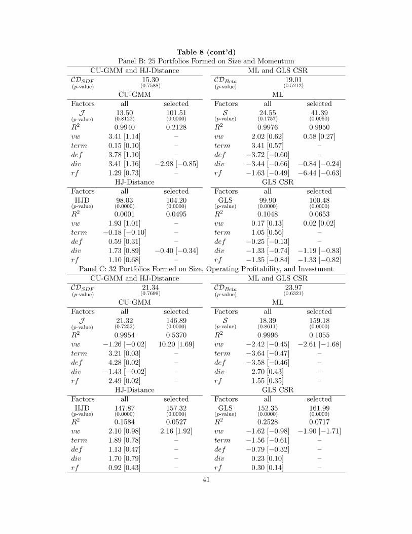
Table 8 (cont’d)Panel B: 25 Portfolios Formed on Size and Momentum

CU-GMM and HJ-Distance ML and GLS CSRCDSDF(p-value)

15.30(0.7588)

CDBeta(p-value)

19.01(0.5212)

CU-GMM MLFactors all selected Factors all selectedJ

(p-value)13.50(0.8122)

101.51(0.0000)

S(p-value)

24.55(0.1757)

41.39(0.0050)

R2 0.9940 0.2128 R2 0.9976 0.9950vw 3.41 [1.14] – vw 2.02 [0.62] 0.58 [0.27]term 0.15 [0.10] – term 3.41 [0.57] –def 3.78 [1.10] – def −3.72 [−0.60] –div 3.41 [1.16] −2.98 [−0.85] div −3.44 [−0.66] −0.84 [−0.24]rf 1.29 [0.73] – rf −1.63 [−0.49] −6.44 [−0.63]

HJ-Distance GLS CSRFactors all selected Factors all selectedHJD

(p-value)98.03(0.0000)

104.20(0.0000)

GLS(p-value)

99.90(0.0000)

100.48(0.0000)

R2 0.0001 0.0495 R2 0.1048 0.0653vw 1.93 [1.01] – vw 0.17 [0.13] 0.02 [0.02]term −0.18 [−0.10] – term 1.05 [0.56] –def 0.59 [0.31] – def −0.25 [−0.13] –div 1.73 [0.89] −0.40 [−0.34] div −1.33 [−0.74] −1.19 [−0.83]rf 1.10 [0.68] – rf −1.35 [−0.84] −1.33 [−0.82]

Panel C: 32 Portfolios Formed on Size, Operating Profitability, and Investment

CU-GMM and HJ-Distance ML and GLS CSRCDSDF(p-value)

21.34(0.7699)

CDBeta(p-value)

23.97(0.6321)

CU-GMM MLFactors all selected Factors all selectedJ

(p-value)21.32(0.7252)

146.89(0.0000)

S(p-value)

18.39(0.8611)

159.18(0.0000)

R2 0.9954 0.5370 R2 0.9996 0.1055vw −1.26 [−0.02] 10.20 [1.69] vw −2.42 [−0.45] −2.61 [−1.68]term 3.21 [0.03] – term −3.64 [−0.47] –def 4.28 [0.02] – def −3.58 [−0.46] –div −1.43 [−0.02] – div 2.70 [0.43] –rf 2.49 [0.02] – rf 1.55 [0.35] –

HJ-Distance GLS CSRFactors all selected Factors all selectedHJD

(p-value)147.87(0.0000)

157.32(0.0000)

GLS(p-value)

152.35(0.0000)

161.99(0.0000)

R2 0.1584 0.0527 R2 0.2528 0.0717vw 2.10 [0.98] 2.16 [1.92] vw −1.62 [−0.98] −1.90 [−1.71]term 1.89 [0.78] – term −1.56 [−0.61] –def 1.13 [0.47] – def −0.79 [−0.32] –div 1.70 [0.79] – div 0.23 [0.10] –rf 0.92 [0.43] – rf 0.30 [0.14] –

41

Table 9Test Statistics for D-CCAPM

The table reports test statistics for D-CCAPM. CDSDF and CDBeta denote the Cragg and Donald (1997)test for the null of a reduced rank in the SDF and beta-pricing setups, respectively. J denotes Hansen,Heaton, and Yaron’s (1996) test for over-identifying restrictions based on the CU-GMM estimator. S denotesShanken’s (1985) Wald-type test of correct model specification based on the ML estimator. HJD and GLSdenote the tests of correct model specification based on the distance measure of Hansen and Jagannathan(1997) and on the generalized least squares cross-sectional regression test of Shanken (1985), respectively. Therows for the different factors report the t-tests of statistical significance with standard errors computed underthe assumption of correct model specification and the misspecification-robust t-tests (in square brackets).Finally, R2 denotes the squared correlation coefficient between the fitted expected returns and the averagerealized returns.

Panel A: 25 Portfolios Formed on Size and Book-to-Market

CU-GMM and HJ-Distance ML and GLS CSRCDSDF(p-value)

25.35(0.2808)

CDBeta(p-value)

35.33(0.0358)

CU-GMM MLFactors all selected Factors all selectedJ

(p-value)20.63(0.4820)

62.20(0.0000)

S(p-value)

28.37(0.1299)

68.79(0.0000)

R2 0.9368 0.2277 R2 0.9762 0.1447vw 3.06 [2.10] 5.28 [3.13] vw −2.17 [−1.77] −3.65 [−2.92]cg −4.73 [−1.55] – cg 5.31 [1.77] –cgdur 0.94 [0.52] – cgdur 2.35 [0.54] –

HJ-Distance GLS CSRFactors all selected Factors all selectedHJD

(p-value)59.65(0.0026)

69.35(0.0000)

GLS(p-value)

61.96(0.0023)

71.96(0.0000)

R2 0.4297 0.0815 R2 0.3642 0.0993vw 3.69 [3.18] 3.35 [3.10] vw −3.09 [−2.93] −3.14 [−2.97]cg −2.42 [−1.66] – cg 2.61 [1.69] –cgdur −0.49 [−0.36] – cgdur 1.09 [0.79] –

42

Table 9 (cont’d)

Panel B: 25 Portfolios Formed on Size and Momentum

CU-GMM and HJ-Distance ML and GLS CSRCDSDF(p-value)

20.37(0.5599)

CDBeta(p-value)

25.86(0.2579)

CU-GMM MLFactors all selected Factors all selectedJ

(p-value)20.11(0.5145)

99.86(0.0000)

S(p-value)

30.15(0.0889)

105.80(0.0000)

R2 0.9870 0.2421 R2 0.9926 0.1128vw 1.69 [0.26] 3.44 [1.23] vw −0.81 [−0.62] −0.95 [−0.68]cg −4.27 [−0.25] – cg −0.07 [−0.00] –cgdur 3.27 [0.22] – cgdur 5.52 [0.22] –

HJ-Distance GLS CSRFactors all selected Factors all selectedHJD

(p-value)92.57(0.0000)

103.54(0.0000)

GLS(p-value)

95.14(0.0000)

106.09(0.0000)

R2 0.2193 0.0702 R2 0.0143 0.0963vw 1.76 [1.33] 0.91 [0.82] vw −1.10 [−0.96] −0.75 [−0.68]cg −1.72 [−1.00] – cg 2.21 [1.24] –cgdur −1.48 [−0.81] – cgdur 2.04 [1.07] –

Panel C: 32 Portfolios Formed on Size, Operating Profitability, and Investment

CU-GMM and HJ-Distance ML and GLS CSRCDSDF(p-value)

21.37(0.8452)

CDBeta(p-value)

23.84(0.7366)

CU-GMM MLFactors all selected Factors all selectedJ

(p-value)21.29(0.8131)

146.89(0.0000)

S(p-value)

29.82(0.3717)

159.18(0.0000)

R2 0.9963 0.5370 R2 0.9990 0.1055vw 2.91 [0.09] 10.20 [1.69] vw 0.08 [0.00] −2.61 [−1.68]cg −4.60 [−0.09] – cg −2.89 [−0.02] –cgdur 1.03 [0.07] – cgdur 4.02 [0.08] –

HJ-Distance GLS CSRFactors all selected Factors all selectedHJD

(p-value)149.60(0.0000)

157.32(0.0000)

GLS(p-value)

154.38(0.0000)

161.99(0.0000)

R2 0.6335 0.0527 R2 0.5117 0.0717vw 2.23 [1.54] 2.16 [1.92] vw −2.14 [−1.83] −1.90 [−1.71]cg −0.69 [−0.32] – cg 1.07 [0.50] –cgdur −1.95 [−1.05] – cgdur 2.32 [1.13] –

43

Table 10Test Statistics for FF3

The table reports test statistics for FF3. CDSDF and CDBeta denote the Cragg and Donald (1997) test forthe null of a reduced rank in the SDF and beta-pricing setups, respectively. J denotes Hansen, Heaton, andYaron’s (1996) test for over-identifying restrictions based on the CU-GMM estimator. S denotes Shanken’s(1985) Wald-type test of correct model specification based on the ML estimator. HJD and GLS denote thetests of correct model specification based on the distance measure of Hansen and Jagannathan (1997) andon the generalized least squares cross-sectional regression test of Shanken (1985), respectively. The rowsfor the different factors report the t-tests of statistical significance with standard errors computed underthe assumption of correct model specification and the misspecification-robust t-tests (in square brackets).Finally, R2 denotes the squared correlation coefficient between the fitted expected returns and the averagerealized returns.

Panel A: 25 Portfolios Formed on Size and Book-to-Market

CU-GMM and HJ-Distance ML and GLS CSRCDSDF(p-value)

109.73(0.0000)

CDBeta(p-value)

298.24(0.0000)

CU-GMM MLFactors all selected Factors all selectedJ

(p-value)44.26(0.0022)

44.26(0.0022)

S(p-value)

51.05(0.0003)

51.05(0.0003)

R2 0.7783 0.7783 R2 0.7337 0.7337vw 4.78 [3.33] 4.78 [3.33] vw −3.80 [−3.03] −3.80 [−3.03]smb −4.60 [−3.48] −4.60 [−3.48] smb 1.73 [1.72] 1.73 [1.72]hml −2.93 [−2.11] −2.93 [−2.11] hml 3.04 [3.03] 3.04 [3.03]

HJ-Distance GLS CSRFactors all selected Factors all selectedHJD

(p-value)53.48(0.0005)

53.48(0.0005)

GLS(p-value)

55.61(0.0004)

55.61(0.0004)

R2 0.6890 0.6890 R2 0.6901 0.6901vw 3.24 [2.95] 3.24 [2.95] vw −3.29 [−3.02] −3.29 [−3.02]smb −3.32 [−3.26] −3.32 [−3.26] smb 1.73 [1.73] 1.73 [1.73]hml −1.96 [−1.96] −1.96 [−1.96] hml 3.04 [3.04] 3.04 [3.04]

44

Table 10 (cont’d)

Panel B: 25 Portfolios Formed on Size and Momentum

CU-GMM and HJ-Distance ML and GLS CSRCDSDF(p-value)

35.09(0.0379)

CDBeta(p-value)

64.60(0.0000)

CU-GMM MLFactors all selected Factors all selectedJ

(p-value)33.71(0.0389)

68.40(0.0000)

S(p-value)

77.55(0.0000)

77.55(0.0000)

R2 0.9869 0.7269 R2 0.8805 0.8805vw 4.71 [0.70] 6.94 [3.17] vw −5.32 [−1.76] −5.32 [−1.76]smb −4.67 [−0.73] −6.86 [−3.48] smb 4.06 [2.84] 4.06 [2.84]hml 5.58 [0.68] – hml −4.63 [−1.48] −4.63 [−1.48]

HJ-Distance GLS CSRFactors all selected Factors all selectedHJD

(p-value)90.29(0.0000)

92.77(0.0000)

GLS(p-value)

93.49(0.0000)

93.49(0.0000)

R2 0.4837 0.2594 R2 0.4934 0.4934vw 2.36 [1.80] 2.20 [1.83] vw −1.88 [−1.48] −1.88 [−1.48]smb −3.06 [−2.72] −3.18 [−2.90] smb 2.99 [2.76] 2.99 [2.76]hml 1.43 [1.05] – hml −1.30 [−0.95] −1.30 [−0.95]

Panel C: 32 Portfolios Formed on Size, Operating Profitability, and Investment

CU-GMM and HJ-Distance ML and GLS CSRCDSDF(p-value)

80.26(0.0000)

CDBeta(p-value)

160.90(0.0000)

CU-GMM MLFactors all selected Factors all selectedJ

(p-value)80.20(0.0000)

80.20(0.0000)

S(p-value)

133.50(0.0000)

133.50(0.0000)

R2 0.9492 0.9492 R2 0.5981 0.5981vw −8.64 [−0.02] −8.64 [−0.02] vw −0.46 [−0.20] −0.46 [−0.20]smb 4.71 [0.02] 4.71 [0.02] smb 0.94 [0.88] 0.94 [0.88]hml −7.86 [−0.02] −7.86 [−0.02] hml 4.66 [2.85] 4.66 [2.85]

HJ-Distance GLS CSRFactors all selected Factors all selectedHJD

(p-value)138.51(0.0000)

138.51(0.0000)

GLS(p-value)

141.97(0.0000)

141.97(0.0000)

R2 0.5766 0.5766 R2 0.5394 0.5394vw 0.60 [0.48] 0.60 [0.48] vw −0.92 [−0.77] −0.92 [−0.77]smb −2.24 [−2.12] −2.24 [−2.12] smb 1.12 [1.09] 1.12 [1.09]hml −3.45 [−2.87] −3.45 [−2.87] hml 3.96 [3.46] 3.96 [3.46]

45

Table 11Test Statistics for HXZ

The table reports test statistics for HXZ. CDSDF and CDBeta denote the Cragg and Donald (1997) test forthe null of a reduced rank in the SDF and beta-pricing setups, respectively. J denotes Hansen, Heaton, andYaron’s (1996) test for over-identifying restrictions based on the CU-GMM estimator. S denotes Shanken’s(1985) Wald-type test of correct model specification based on the ML estimator. HJD and GLS denote thetests of correct model specification based on the distance measure of Hansen and Jagannathan (1997) andon the generalized least squares cross-sectional regression test of Shanken (1985), respectively. The rowsfor the different factors report the t-tests of statistical significance with standard errors computed underthe assumption of correct model specification and the misspecification-robust t-tests (in square brackets).Finally, R2 denotes the squared correlation coefficient between the fitted expected returns and the averagerealized returns.

Panel A: 25 Portfolios Formed on Size and Book-to-Market

CU-GMM and HJ-Distance ML and GLS CSRCDSDF(p-value)

42.60(0.0035)

CDBeta(p-value)

93.98(0.0000)

CU-GMM MLFactors all selected Factors all selectedJ

(p-value)42.11(0.0027)

42.11(0.0027)

S(p-value)

50.72(0.0002)

50.72(0.0002)

R2 0.8162 0.8162 R2 0.7607 0.7607vw 2.89 [2.12] 2.89 [2.12] vw −3.29 [−2.25] −3.29 [−2.25]me −4.86 [−3.44] −4.86 [−3.44] me 2.53 [2.37] 2.53 [2.37]roe −2.30 [−1.19] −2.30 [−1.19] roe 1.65 [1.03] 1.65 [1.03]ia −1.73 [−1.00] −1.73 [−1.00] ia 2.72 [2.05] 2.72 [2.05]

HJ-Distance GLS CSRFactors all selected Factors all selectedHJD

(p-value)54.01(0.0003)

54.01(0.0003)

GLS(p-value)

56.09(0.0003

56.09(0.0003)

R2 0.7204 0.7204 R2 0.6938 0.6938vw 2.23 [1.96] 2.23 [1.96] vw −2.98 [−2.67] −2.98 [−2.67]me −3.62 [−3.42] −3.62 [−3.42] me 2.38 [2.34] 2.38 [2.34]roe −1.23 [−1.06] −1.23 [−1.06] roe 1.24 [1.06] 1.24 [1.06]ia −1.18 [−1.07] −1.18 [−1.07] ia 2.54 [2.35] 2.54 [2.35]

46

Table 11 (cont’d)

Panel B: 25 Portfolios Formed on Size and Momentum

CU-GMM and HJ-Distance ML and GLS CSRCDSDF(p-value)

37.19(0.0160)

CDBeta(p-value)

51.59(0.0002)

CU-GMM MLFactors all selected Factors all selectedJ

(p-value)30.62(0.0604)

67.90(0.0000)

S(p-value)

51.56(0.0001)

51.56(0.0001)

R2 0.9694 0.7263 R2 0.9347 0.9347vw −3.98 [−1.51] 7.04 [3.45] vw 3.21 [0.75] 3.21 [0.75]me −3.41 [−1.28] −6.93 [−3.68] me 3.80 [3.60] 3.80 [3.60]roe −4.67 [−2.06] – roe 3.71 [1.81] 3.71 [1.81]ia −4.47 [−1.67] – ia 3.35 [0.66] 3.35 [0.66]

HJ-Distance GLS CSRFactors all selected Factors all selectedHJD

(p-value)64.98(0.0008)

93.45(0.0000)

GLS(p-value)

65.79(0.0009)

65.79(0.0009)

R2 0.9086 0.2628 R2 0.8784 0.8784vw −0.82 [−0.60] 2.02 [1.67] vw 0.74 [0.58] 0.74 [0.58]me −4.24 [−4.20] −3.13 [−2.89] me 3.46 [3.41] 3.46 [3.41]roe −3.30 [−3.17] – roe 3.23 [3.17] 3.23 [3.17]ia −1.08 [−0.79] – ia 0.96 [0.71] 0.96 [0.71]

Panel C: 32 Portfolios Formed on Size, Operating Profitability, and Investment

CU-GMM and HJ-Distance ML and GLS CSRCDSDF(p-value)

50.50(0.0057)

CDBeta(p-value)

122.10(0.0000)

CU-GMM MLFactors all selected Factors all selectedJ

(p-value)28.54(0.3836)

28.54(0.3836)

S(p-value)

69.36(0.0000)

69.36(0.0000)

R2 0.9472 0.9472 R2 0.8810 0.8810vw −4.90 [−2.58] −4.90 [−2.58] vw 2.94 [1.80] 2.94 [1.80]me −1.67 [−0.94] −1.67 [−0.94] me 3.59 [3.40] 3.59 [3.40]roe −6.46 [−3.48] −6.46 [−3.48] roe 6.74 [4.45] 6.74 [4.45]ia −6.27 [−3.66] −6.27 [−3.66] ia 6.42 [5.65] 6.42 [5.65]

HJ-Distance GLS CSRFactors all selected Factors all selectedHJD

(p-value)101.22(0.0001)

101.22(0.0001)

GLS(p-value)

102.44(0.0001)

102.44(0.0001)

R2 0.8325 0.8325 R2 0.7499 0.7499vw −1.99 [−1.85] −1.99 [−1.85] vw 0.90 [0.82] 0.90 [0.82]me −4.03 [−3.87] −4.03 [−3.87] me 2.97 [2.86] 2.97 [2.86]roe −4.24 [−4.26] −4.24 [−4.26] roe 4.63 [4.56] 4.63 [4.56]ia −4.41 [−4.36] −4.41 [−4.36] ia 5.73 [5.57] 5.73 [5.57]

47

Annualized Fitted Return (in %)

0 5 10 15 20

Annualized

RealizedReturn

(in%)

0

5

10

15

20CAPM

45 lineFF25 Portfolios

Annualized Fitted Return (in %)

0 5 10 15 20

Annualized

RealizedReturn

(in%)

0

5

10

15

20FF3

45 lineFF25 Portfolios

Annualized Fitted Return (in %)

0 5 10 15 20

Annualized

RealizedReturn

(in%)

0

5

10

15

20C-LAB

45 lineFF25 Portfolios

Annualized Fitted Return (in %)

0 5 10 15 20

Annualized

RealizedReturn

(in%)

0

5

10

15

20CC-CAY

45 lineFF25 Portfolios

Figure 1. Realized vs. Fitted (by CU-GMM) Returns: 25 Fama-French Portfolios. Thefigure shows the average realized returns versus fitted expected returns (by CU-GMM) for each ofthe 25 Fama-French portfolios for CAPM, FF3, C-LAB, and CC-CAY.

48

Annualized Fitted Return (in %)

0 5 10 15 20

Annualized

RealizedReturn

(in%)

0

5

10

15

20CAPM

45 lineFF25 Portfolios

Annualized Fitted Return (in %)

0 5 10 15 20

Annualized

RealizedReturn

(in%)

0

5

10

15

20FF3

45 lineFF25 Portfolios

Annualized Fitted Return (in %)

0 5 10 15 20

Annualized

RealizedReturn

(in%)

0

5

10

15

20C-LAB

45 lineFF25 Portfolios

Annualized Fitted Return (in %)

0 5 10 15 20

Annualized

RealizedReturn

(in%)

0

5

10

15

20CC-CAY

45 lineFF25 Portfolios

Figure 2. Realized vs. Fitted (by ML) Returns: 25 Fama-French Portfolios. The figureshows the average realized returns versus fitted expected returns (by ML) for each of the 25 Fama-French portfolios for CAPM, FF3, C-LAB, and CC-CAY.

49

Annualized Fitted Return (in %)

0 5 10 15 20

Annualized

RealizedReturn

(in%)

0

5

10

15

20CAPM

45 lineFF25 Portfolios

Annualized Fitted Return (in %)

0 5 10 15 20

Annualized

RealizedReturn

(in%)

0

5

10

15

20FF3

45 lineFF25 Portfolios

Annualized Fitted Return (in %)

0 5 10 15 20

Annualized

RealizedReturn

(in%)

0

5

10

15

20C-LAB

45 lineFF25 Portfolios

Annualized Fitted Return (in %)

0 5 10 15 20

Annualized

RealizedReturn

(in%)

0

5

10

15

20CC-CAY

45 lineFF25 Portfolios

Figure 3. Realized vs. Fitted (by HJ-Distance) Returns: 25 Fama-French Portfolios.The figure shows the average realized returns versus fitted expected returns (by HJ-distance) foreach of the 25 Fama-French portfolios for CAPM, FF3, C-LAB, and CC-CAY.

50

Annualized Fitted Return (in %)

0 5 10 15 20

Annualized

RealizedReturn

(in%)

0

5

10

15

20CAPM

45 lineFF25 Portfolios

Annualized Fitted Return (in %)

0 5 10 15 20

Annualized

RealizedReturn

(in%)

0

5

10

15

20FF3

45 lineFF25 Portfolios

Annualized Fitted Return (in %)

0 5 10 15 20

Annualized

RealizedReturn

(in%)

0

5

10

15

20C-LAB

45 lineFF25 Portfolios

Annualized Fitted Return (in %)

0 5 10 15 20

Annualized

RealizedReturn

(in%)

0

5

10

15

20CC-CAY

45 lineFF25 Portfolios

Figure 4. Realized vs. Fitted (by GLS) Returns: 25 Fama-French Portfolios. The figureshows the average realized returns versus fitted expected returns (by GLS) for each of the 25Fama-French portfolios for CAPM, FF3, C-LAB, and CC-CAY.

51

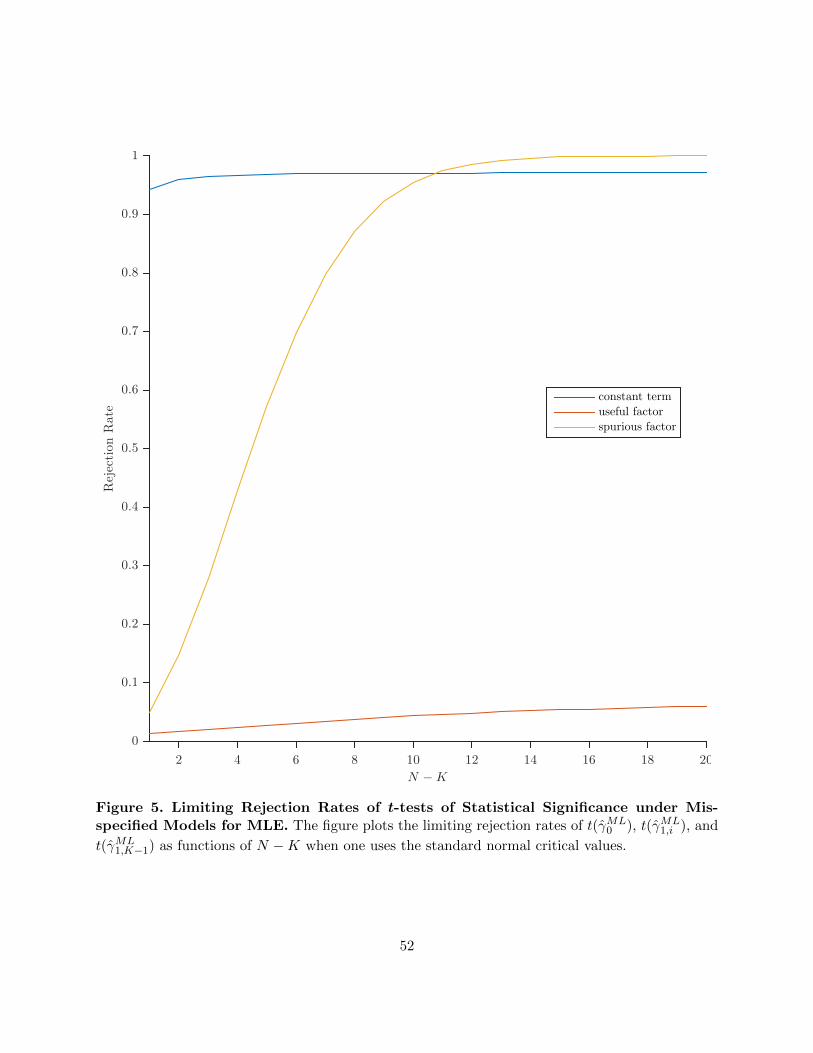
N −K

2 4 6 8 10 12 14 16 18 20

RejectionRate

0

0.1

0.2

0.3

0.4

0.5

0.6

0.7

0.8

0.9

1

constant term

useful factor

spurious factor

Figure 5. Limiting Rejection Rates of t-tests of Statistical Significance under Mis-specified Models for MLE. The figure plots the limiting rejection rates of t(γML

0 ), t(γML1,i ), and

t(γML1,K−1) as functions of N −K when one uses the standard normal critical values.

52

N −K

2 4 6 8 10 12 14 16 18 20

RejectionRate

0

0.2

0.4

0.6

0.8

1

constant term

useful factor

spurious factor

N −K

2 4 6 8 10 12 14 16 18 20

RejectionRate

0

0.2

0.4

0.6

0.8

1

spurious factor: correctly specified model

spurious factor: misspecified model

Figure 6. Limiting Rejection Rates of t-tests of Statistical Significance for CU-GMM.The top graph plots the limiting rejection rates under misspecified models of t(λ0) (with µf,K−1 =

0), t(λ1,i), and t(λ1,K−1) as functions of N −K when one uses the standard normal critical values.The bottom graph plots the limiting rejection rates under correctly specified and misspecifiedmodels of t(λ1,K−1) as functions of N −K when one uses the standard normal critical values.

53

−5 −4 −3 −2 −1 0 1 2 3 4 50

0.05

0.1

0.15

0.2

0.25

0.3

0.35

0.4

t-statistic

ProbabilityDensity

Function

Correctly Specified ModelMisspecified ModelN (0, 1)

Figure 7. Limiting Distributions of t(λ1,K−1) under Correctly Specified and Misspec-

ified Models. The figure plots the limiting densities of t(λ1,K−1) for correctly specified andmisspecified models that contain a spurious factor (for N − K = 7), along with the standardnormal density.

54

Online Appendix to

“Too Good to Be True? Fallacies in Evaluating Risk

Factor Models”

Nikolay Gospodinov, Raymond Kan, and Cesare Robotti

This Online Appendix is structured as follows. Appendix A contains proofs of the theorems.

Appendix B provides details on the CU-GMM estimation of the beta-pricing model. We refer the

readers to the paper for the notation used here.

Appendix A: Proofs of Theorems

A.1 Auxiliary Lemma 1

Auxiliary Lemma 1. Let z = [z1, z2, . . . , zK ]′ ∼ N (0K , (G′1Σ−1G1)

−1/σ2f,K−1), where G1 =

[1N , α, β1, . . . , βK−2] and σ2f,K−1 = Var[fK−1,t]. Assume that Yt is iid normally distributed.

Suppose that the model is misspecified and it contains a useless factor (that is, rank(B) = K − 1).

Then, T → ∞, we have (i) γML0

d→ −z1z2

; (ii) γML1,i

d→ µf,i −zi+2

z2for i = 1, . . . ,K − 2; and (iii)

γML1,K−1√T

d→ 1

z2.

Proof. When the model is misspecified and contains a useless factor (ordered last), we have

Gv∗ = 0N for v∗ = [0′K , 1]′. Let v be the eigenvector associated with the largest eigenvalue of

Ω = (G′Σ−1G)−1[A(X ′X/T )−1A′]. (A.1)

Define ψ = [ψ1, ψ2, . . . , ψK ]′ as

ψi = − vivK+1

, i = 1, . . . ,K, (A.2)

which is asymptotically equivalent to the estimator

ψ = (G′1Σ−1G1)

−1(G′1Σ−1βK−1). (A.3)

Since√T βK−1

d→ N (0N ,Σ/σ2f,K−1), we have

√T ψ

d→ N (0K , (G′1Σ−1G1)

−1/σ2f,K1), (A.4)

and√T ψ also has the same asymptotic distribution. Therefore, we can write

γML0 = −

√T ψ1√T ψ2

d→ −z1z2, (A.5)

γML1,i = µf,i −

√T ψi+2√T ψ2

d→ µf,i −zi+2

z2, i = 1, . . . ,K − 2, (A.6)

γML1,K−1√T

=µf,K−1√

T+

1√T ψ2

d→ 1

z2. (A.7)

This completes the proof of the lemma.

1

A.2 Proof of Theorem 1

part (a): Let σ2i = Var[zi], σij ≡ Cov[zi, zj ], ρij = σij/(σiσj), G2 = [1N , β1, . . . , βK−2], G2 =

[1N , β1, . . . , βK−2], and define the random variables z2 ≡ z2/σ2 ∼ N (0, 1), x ∼ χ2N−K , qi ∼ N (0, 1),

where x and qi are independent of z2, and bi = (x + z22)/(x + z22 + q2i ) for i = 1, . . . ,K − 1. We

start with the squared t-ratio of the useless factor, t2(γML1,K−1). Using the formula for the inverse of

a partitioned matrix, we obtain

s2(γML1,K−1) = (1 + γML′

1 V −1f γML1 )

(β′K−1[Σ

−1 − Σ−1G2(G′2Σ−1G2)

−1G′2Σ−1]βK−1

)−1+ σ2f,K−1

=

(γML1,K−1σf,K−1

)2 (β′K−1[Σ

−1 − Σ−1G2(G′2Σ−1G2)

−1G′2Σ−1]βK−1

)−1+Op(T

12 ) (A.8)

by using the fact that γML1,i = Op(1) for i = 1, . . . ,K − 2 and γML

1,K−1 = Op(T12 ). In addition, by

defining u as follows:√T σf,K−1Σ

− 12 βK−1

d→ u ∼ N (0N , IN ), (A.9)

we obtain

t2(γML1,K−1) =

T (γML1,K−1)

2β′K−1[Σ

−1 − Σ−1G2(G′2Σ−1G2)

−1G2Σ−1]βK−1

(γML1,K−1/σf,K−1)

2+Op(T

− 12 )

= u′[IN − Σ−12 G2(G

′2Σ−1G2)

−1G′2Σ− 1

2 ]u+Op(T− 1

2 )

d→ u′[IN − Σ−12G2(G

′2Σ−1G2)

−1G′2Σ− 1

2 ]u ∼ χ2N−K+1. (A.10)

For the limiting distributions of t(γML0 ) and t(γML

1,i ), i = 1, . . . ,K − 2, we use the formula for

the inverse of a partitioned matrix to obtain the upper left (K−1)× (K−1) block of (B′1Σ−1B1)

−1

as

(G′2Σ−1G2)

−1 +(G′2Σ

−1G2)−1G′2Σ

−1βK−1β′K−1Σ

−1G2(G′2Σ−1G2)

−1

β′K−1Σ

−1βK−1 − β′K−1Σ

−1G2(G′2Σ−1G2)−1G′2Σ

−1βK−1

= (G′2Σ−1G2)

−1 +(G′2Σ

−1G2)−1G′2Σ

− 12uu′Σ−

12G2(G

′2Σ−1G2)

−1

u′[IN − Σ−12G2(G′2Σ

−1G2)−1G′2Σ− 1

2 ]u+Op(T

− 12 ). (A.11)

Note that we can write

IN − Σ−12G1(G

′1Σ−1G1)

−1G′1Σ− 1

2 = IN − Σ−12G2(G

′2Σ−1G2)

−1G′2Σ− 1

2 − hh′, (A.12)

where

h =[IN − Σ−

12G2(G

′2Σ−1G2)

−1G′2Σ− 1

2 ]Σ−12α(

α′Σ−12 [IN − Σ−

12G2(G′2Σ

−1G2)−1G′2Σ− 1

2 ]Σ−12α) 1

2

. (A.13)

2

With this expression, we can write

u′[IN − Σ−12G2(G

′2Σ−1G2)

−1G′2Σ− 1

2 ]u = u′[IN − Σ−12G1(G

′1Σ−1G1)

−1G′1Σ− 1

2 ]u+ (h′u)2

= x+ z22 , (A.14)

where x ∼ χ2N−K and it is independent of z2 ∼ N (0, 1). To establish the last equality, we need

to show that h′u = z2. Denote by ιm,i an m-vector with its i-th element equals to one and zero

elsewhere, and let σi,j ≡ Cov[zi, zj ] = ι′K,i(G′1Σ−1G1)

−1ιK,j/σ2f,K−1. Using the formula for the

inverse of a partitioned matrix, we obtain

z2 =1

σf,K−1ι′K,2(G

′1Σ−1G1)

−1G′1Σ− 1

2u

=1

σf,K−1

α′Σ−12 [IN − Σ−

12G2(G

′2Σ−1G2)

−1G′2Σ− 1

2 ]u

α′Σ−12 [IN − Σ−

12G2(G′2Σ

−1G2)−1G′2Σ− 1

2 ]Σ−12α. (A.15)

It follows that

σ22 =1

σ2f,K−1α′Σ−

12 [IN − Σ−

12G2(G′2Σ

−1G2)−1G′2Σ− 1

2 ]Σ−12α

(A.16)

and h′u = z2/σ2 = z2.

Denote by wi the i-th diagonal element of (B′1Σ−1B1)

−1, i = 1, . . . ,K − 1. Using (A.11), we

have

wid→ ι′K−1,i(G

′2Σ−1G2)

−1ιK−1,i +ι′K−1,i(G

′2Σ−1G2)

−1G′2Σ− 1

2uu′Σ−12G2(G

′2Σ−1G2)

−1ιK−1,i

x+ z22

= ι′K−1,i(G′2Σ−1G2)

−1ιK−1,i

(1 +

q2ix+ z22

), (A.17)

where

qi =ι′K−1,i(G

′2Σ−1G2)

−1G′2Σ− 1

2u

[ι′K−1,i(G′2Σ−1G2)−1ιK−1,i]

12

∼ N (0, 1). (A.18)

Using the fact that Var[u] = IN and

(G′1Σ−1G1)

−1G′1Σ−1G2 = [ιK,1, ιK,3, . . . , ιK,K ], (A.19)

it is straightforward to show that

Cov[z1, q1] =ι′K,1(G

′1Σ−1G1)

−1G′1Σ−1G2(G

′2Σ−1G2)

−1ιK−1,1

σf,K−1[ι′K−1,1(G

′2Σ−1G2)−1ιK−1,1]

12

= [ι′K−1,1(G′2Σ−1G2)

−1ιK−1,1/σ2f,K−1]

12 , (A.20)

Cov[z2, q1] =ι′K,2(G

′1Σ−1G1)

−1G′1Σ−1G2(G

′2Σ−1G2)

−1ιK−1,1

σf,K−1[ι′K−1,1(G

′2Σ−1G2)−1ιK−1,1]

12

= 0. (A.21)

3

From the formula for the inverse of a partitioned matrix, we have

1

σ2f,K−1ι′K−1,1(G

′2Σ−1G2)

−1ιK−1,1 = σ21 −σ21,2σ22

= σ21(1− ρ21,2). (A.22)

It follows that

Cov

[z1 −

σ12σ22

z2, q1

]= [ι′K−1,1(G

′2Σ−1G2)

−1ιK−1,1/σ2f,K−1]

12 = σ1

√1− ρ21,2. (A.23)

Therefore, z1 − (σ1,2/σ22)z2 is perfectly correlated with q1 and we can write

z1 =σ1,2σ22

z2 +√

1− ρ21,2σ1q1 = σ1

(ρ1,2z2 +

√1− ρ21,2q1

). (A.24)

Similarly,

zi+1 =σi+1,2

σ22z2+

√1− ρ2i+1,2σi+1qi = σi+1

(ρi+1,2z2 +

√1− ρ2i+1,2qi

), i = 2, . . . ,K−1. (A.25)

Let

bi =x+ z22

x+ z22 + q2i, i = 1, . . . ,K − 1. (A.26)

With the above results, we can now write the limiting distribution of the t-ratios as

t(γML0 )

d→ − z1|z2|b121

z2[ι′K−1,1(G′2Σ−1G2)−1ιK−1,1/σ2f,K−1]

12

= −

ρ1,2|z2|√1− ρ21,2

+ q1

b121 , (A.27)

t(γML1,i )

d→

(µf,i −

zi+2

z2

)|z2|b

12i+1

[ι′K−1,i+1(G′2Σ−1G2)−1ιK−1,i+1/σ2f,K−1]

12

=

µf,iσ2

σi+2− ρi+2,2√

1− ρ2i+2,2

|z2| − qi+1

b12i+1, i = 1, . . . ,K − 2. (A.28)

Defining Z0 = −

(ρ1,2|z2|√1−ρ21,2

+ q1

)b121 and Zi =

(µf,iσ2σi+2

−ρi+2,2√1−ρ2i+2,2

|z2| − qi+1

)b12i+1 for i = 1, . . . ,K − 2,

delivers the desired result. This completes the proof of part (a).

part (b): Let e = µR− 1N γML0 − βγML

1 and note that the fitted (model-implied) expected returns

4

can be rewritten as

µMLR = 1N γ

ML0 + β

MLγML1

= 1N γML0 + βγML

1 + eγML′1 V −1f γML

1

1 + γML′1 V −1f γML

1

= µR − e+ eγML′1 V −1f γML

1

1 + γML′1 V −1f γML

1

= µR − e1

1 + γML′1 V −1f γML

1

. (A.29)

Using the result from Auxiliary Lemma 1 that γML1,i = Op(1) for i = 1, . . . ,K − 2 and γML

1,K−1 =

Op(T12 ), we have µML

R − µRp→ 0N and

R2ML = Corr(µML

R , µR)2p→ 1 (A.30)

as T →∞. This completes the proof of part (b).

A.3 Auxiliary Lemma 2

Auxiliary Lemma 2. Let z = [z1, z2, . . . , zK ]′ ∼ N (0K , σ2f,K−1(H

′1U−1H1)

−1), where H1 =

[1N , D1] and D1 = [d1, d2, . . . , dK−1] with di ( i = 1, . . . ,K) being the i-th column of D. Assume

that Yt is a jointly stationary and ergodic process with a finite fourth moment, vec(Dt −D) : t ≥ 1is a martingale difference sequence. Suppose that the model is misspecified and it contains a useless

factor (that is, rank(D) = K − 1). Then, T → ∞, we have (i) λ0d→ −z2

z1if µf,K−1 = 0 or

λ0√T

d→µf,K−1z1

if µf,K−1 6= 0; (ii) λ1,id→ −zi+2

z1for i = 1, . . . ,K − 2; and (iii)

λ1,K−1√T

d→ − 1

z1.

Proof. We first perform the following parameterization of the problem. Let

gt(v) = Ht

[v1

]. (A.31)

When the spurious factor is ordered last, we have that E[RtfK−1,t] = µRµf,K−1 andH[v∗′, 1]′ = 0N ,

where

v∗ =

0−µf,K−1

0K−2

. (A.32)

Consider the CU-GMM estimator of v∗:

v = argminv g(v)′Wg(v)−1g(v), (A.33)

5

where g(v) =∑T

t=1 gt(v)/T and Wg(v) = 1T

∑Tt=1[gt(v) − g(v)][gt(v) − g(v)]′. The asymptotic

distribution of v is given by

√T (v − v∗) d→ N

(0K , (H

′1S−1g H1)

−1) , (A.34)

where

Sg = E[gt(v∗)gt(v

∗)′] = E[RtR′t(fK−1,t − µf,K−1)2] = Uσ2f,K−1, (A.35)

and U = E[RtR′t]. Note that v has the same asymptotic distribution as the estimator

v = (H ′1U−1H1)

−1H ′1U−1dK . (A.36)

Let

z ∼ N (0K , σ2f,K−1(H

′1U−1H1)

−1). (A.37)

Then, we have

√T v1

d→ z1, (A.38)√T (v2 + µf,K−1)

d→ z2, (A.39)√T vi

d→ zi, i = 3, . . . ,K. (A.40)

Due to the invariance property of CU-GMM, we know that [−1, λ′] is proportional to [v′, 1]. Then,

we have λ0 = − v2v1

, λ1,i = − vi+2

v1for i = 1, . . . ,K − 2, and λ1,K−1 = − 1

v1. Therefore, the limiting

distributions of the K − 1 elements of λ1 are given by

λ1,id→ −zi+2

z1, i = 1, . . . ,K − 2, (A.41)

λ1,K−1√T

d→ − 1

z1. (A.42)

The limiting distribution of λ0 depends on whether µf,K−1 = 0 or not. If µf,K−1 = 0, we have

λ0d→ −z2/z1. If µf,K−1 6= 0, we have λ0/

√T

d→ µf,K−1/z1. This completes the proof of the lemma.

A.4 Proof of Theorem 2

part (a): It is easy to show that

σ21 =σ2f,K−1

1′N [U−1 − U−1D1(D′1U−1D1)−1D′1U

−1]1N=σ2f,K−1

δ2, (A.43)

where δ is the HJ-distance of the misspecified model. Then,

λ1,K−1√T

d→ − 1

σ1z1= − δ

σf,K−1z1, (A.44)

6

where z1 = z1/σ1 ∼ N (0, 1). Using the fact that

et(λ)√T

= −Rt(fK−1,t − µf,K−1)

z1+Op(T

− 12 ), (A.45)

we can show thatWe(λ)

T=σ2f,K−1z21

U + op(1). (A.46)

This allows us to show that the squared t-ratio of λ1,K−1 can be expressed as

t2(λ1,K−1) =T λ

2

1,K−1

ι′K,K(D′We(λ)−1D)−1ιK,K

=T d′K [U−1 − U−1D1(D

′1U−1D1)

−1D′1U−1]dK

σ2f,K−1+ op(1), (A.47)

where ιK,K is a generic K×1 selector vector with one for its K-th element and zero otherwise. Let

dK = dK − µRµf,K−1 =1

T

T∑t=1

Rt(fK−1,t − µf,K−1). (A.48)

Then, we have√T dK

d→ N (0N , σ2f,K−1U). Since µRµf,K−1 = D1[µf,K−1, 0′K−2]

′, it follows that

T d′K [U−1 − U−1D1(D′1U−1D1)

−1D′1U−1]dK = T d′K [U−1 − U−1D1(D

′1U−1D1)

−1D′1U−1]dK

= T d′K [U−1 − U−1D1(D′1U−1D1)

−1D′1U−1]dK + op(1). (A.49)

Let PU be an N × (N −K + 1) orthonormal matrix with its columns orthogonal to U−12D1. Then,

1

σf,K−1

√TP ′UU

− 12 dK

d→ N (0N−K+1, IN−K+1) (A.50)

and

t2(λ1,K−1)d→ χ2

N−K+1. (A.51)

For the derivation of the limiting distributions for t(λ0) and t(λ1,i) (i = 1, . . . ,K − 2), we use

the identity

IN − U−12H1(H

′1U−1H1)

−1H ′1U− 1

2 = IN − U−12D1(D

′1U−1D1)

−1D′1U− 1

2 − hh′, (A.52)

where

h =[IN − U−

12D1(D

′1U−1D1)

−1D′1U− 1

2 ]U−12 1N

δ=PUP

′UU− 1

2 1Nδ

(A.53)

and h′h = 1. Note that

√Th′U−

12 dK/σf,K−1 =

√T1′NU

− 12PUP

′UU− 1

2 dK/(σf,K−1δ)d→ z1 ∼ N (0, 1), (A.54)

T d′K [IN − U−12H1(H

′1U−1H1)

−1H ′1U− 1

2 ]dK/σ2f,K−1

d→ x ∼ χ2N−K , (A.55)

7

and they are independent of each other. Using the formula for the inverse of a partitioned matrix,

we can show that

σ2f,K−1ι′K−1,i(D

′1U−1D1)

−1ιK−1,i = σ2i+1 −σ1,i+1

σ21= σ2i+1(1− ρ21,i+1), (A.56)

where σ2i = Var[zi], σi,j ≡ Cov[zi, zj ], and ρi,j = σi,j/(σiσj). In addition, we can easily show that

for i = 2, . . . ,K − 1

√Tι′K−1,i(D

′1U−1D1)

−1D′1U−1dK

σf,K−1[ι′K−1,i(D

′1U−1D1)−1ιK−1,i]

12

d→ qi+1 ∼ N (0, 1). (A.57)

For i = 1, the result depends on whether µf,K−1 = 0 or not. If µf,K−1 = 0, we have√TU−

12 dK/σf,K−1

d→ N (0N , IN ) and hence

√Tι′K−1,1(D

′1U−1D1)

−1D′1U−1dK

σf,K−1[ι′K−1,1(D

′1U−1D1)−1ιK−1,1]

12

d→ q2 ∼ N (0, 1). (A.58)

Note that the qi’s are independent of z1 and x. If µf,K−1 6= 0, we have dKp→ µRµf,K−1 =

D1[µf,K−1, 0′K−2]′ and hence

ι′K−1,1(D′1U−1D1)

−1D′1U−1dK/σf,K−1

p→ ι′K−1,1(D′1U−1D1)

−1D′1U−1D1[µf,K−1, 0′K−2]

′/σf,K−1

= µf,K−1/σf,K−1. (A.59)

Consider the upper left (K − 1) × (K − 1) submatrix of (D′We(λ)−1D)−1/T , which has the

same limit as

σ2f,K−1z21

[(D′1U

−1D1)−1 +

(D′1U−1D1)

−1D′1U−1dK d

′KU−1D1(D

′1U−1D1)

−1

d′KU− 1

2 [IN − U−12D1(D′1U

−1D1)−1D′1U− 1

2 ]U−12 dK

]. (A.60)

In particular, for i = 2, . . . ,K−1, the i-th diagonal element of this matrix has a limiting distribution

σ2f,K−1ι′K−1,i(D

′1U−1D1)

−1ιK−1,i

z21

(1 +

q2i+1

x+ z21

)=σ2i+1(1− ρ21,i+1)

z21

(1 +

q2i+1

x+ z21

). (A.61)

Let

bi+1 =x+ z21

q2i+1 + x+ z21(A.62)

and note that, using the same arguments as in the proof of part (b) in Theorem 1, we can write

zi+1 = σi+1

(ρ1,i+1z1 +

√1− ρ21,i+1qi+1

). (A.63)

8

Then, the limiting distribution of t(λ1,i) for i = 1, . . . ,K − 2 can be expressed as

t(λ1,i)d→ − zi+2/z1

σi+2

√1− ρ21,i+2|z1|b

− 12

i+1

= −|z1|z1

(ρ1,i+2z1 +

√1− ρ21,i+2qi+2

)b12i+1√

1− ρ21,i+2

= −

ρ1,i+2|z1|√1− ρ21,i+2

+ qi+2

b12i+1. (A.64)

The limiting distribution of t(λ0) depends on whether µf,K−1 = 0 or not. If µf,K−1 = 0, we have

a similar limiting expression

t(λ0)d→ −

ρ1,2|z1|√1− ρ21,2

+ q2

b121 . (A.65)

Defining Zi = −

(ρ1,i+2|z1|√1−ρ21,i+2

+ qi+2

)b12i+1 for i = 0, . . . ,K−2, delivers the desired result. If µf,K−1 6=

0, we have

t2(λ0)d→

µ2f,K−1

z21

σ2f,K−1

z21

[µ2f,K−1

σ2f,K−1(x+z

21)

] = x+ z21 ∼ χ2N−K+1. (A.66)

This completes the proof of part (a).

part (b): The proof follows similar arguments as the proof of part (b) in Theorem 1 by replacing

the expression for βML

with the expression for βCU

and, to conserve space, is omitted.

Appendix B: CU-GMM Estimation of the Beta-Pricing Model

Let φ = [γ0, γ′1, β

′1, . . . , β

′K , µ

′f , vech(Vf )′]′ denote the vector of parameters of interest, where βi

is an N × 1 vector. In addition, let

gt(φ) =

Rt − (1Nγ0 + βγ1)− β(ft − µf )

[Rt − (1Nγ0 + βγ1)− β(ft − µf )]⊗ ftft − µf

vech((ft − µf )(ft − µf )′ − Vf

) (B.1)

and note that E[gt(φ)] = 0(N+1)(K+1)+(K+1)K/2−1. Finally, let g(φ) = T−1∑T

t=1 gt(φ) and

Wg(φ) =1

T

T∑t=1

(gt(φ)− g(φ))(gt(φ)− g(φ))′. (B.2)

9

Then, the CU-GMM estimator of φ is defined as

φ = argminφ g(φ)′Wg(φ)−1g(φ). (B.3)

The problem with implementing this CU-GMM estimator is that the parameter vector φ is

high dimensional especially when the number of test assets N is large. Penaranda and Sentana

(2015) show that CU-GMM delivers numerically identical estimates in the beta-pricing and linear

SDF setups.1 By augmenting E[et(λ)] in the SDF representation with additional (just-identified)

moment conditions for µf , Vf , and β, the CU-GMM estimate of the augmented parameter vector

θ = [λ0, λ′1, β

′1, . . . , β

′K , µ

′f , vech(Vf )′]′ becomes numerically identical to the CU-GMM estimate of

φ in the beta-pricing model. However, the estimation of θ can be performed in a sequential manner

which offers substantial computational advantages. The following lemma presents a general result

for this sequential estimation.

Lemma B.1. Let θ = [θ′1, θ′2]′, where θ1 is K1 × 1 and θ2 is K2 × 1, and

E[gt(θ)] =

[E[g1t(θ1)]E[g2t(θ)]

]=

[0N1

0N2

], (B.4)

where g1t(θ1) is N1 × 1 and g2t(θ) is N2 × 1, with N1 > K1 and N2 = K2. Define the estimators

θ1 = argminθ1 g1(θ1)′W11(θ1)

−1g1(θ1), (B.5)

θ ≡[θ1θ2

]= argminθ g(θ)′W (θ)−1g(θ), (B.6)

where g1(θ1) = 1T

∑Tt=1 g1t(θ1), W11(θ1) = 1

T

∑Tt=1(g1t(θ1) − g1(θ1))(g1t(θ1) − g1(θ1))

′, g(θ) =

1T

∑Tt=1 gt(θ), and W (θ) = 1

T

∑Tt=1(gt(θ)− g(θ))(gt(θ)− g(θ))′. Then, θ1 = θ1.

Proof. Let

D11(θ1) =1

T

T∑t=1

wt(θ1)∂g1t(θ1)

∂θ′1, (B.7)

where

wt(θ1) = 1− g1(θ1)′W11(θ1)−1[g1t(θ1)− g1(θ1)]. (B.8)

The first-order conditions for the smaller system are given by

D11(θ1)′W11(θ1)

−1g1(θ1) = 0N1 . (B.9)

1Shanken and Zhou (2007) show that under some particular Kronecker structure for the weighting matrix Wg, theGMM estimator of the beta-pricing model is numerically identical to the ML estimator.

10

Similarly, we define

D(θ) =1

T

T∑t=1

wt(θ)∂gt(θ)

∂θ′≡[D11(θ) 0N1×N2

D21(θ) D22(θ)

], (B.10)

where

wt(θ) = 1− g(θ)′W (θ)−1[gt(θ)− g(θ)]. (B.11)

The first-order conditions for the larger system are given by

D(θ)′W (θ)−1g(θ) = 0N1+N2 . (B.12)

Let

W (θ)−1 =

[W 11(θ) W 12(θ)

W 21(θ) W 22(θ)

]. (B.13)

Suppressing the dependence on the parameters in D(θ) and W (θ), the first-order conditions for the

larger system can be written as

0N1+N2 = D(θ)′W (θ)−1g(θ)

=

[(D′11W

11 + D′21W21)g1(θ1) + (D′11W

12 + D′21W22)g2(θ)

D′22W21g1(θ1) + D′22W

22g2(θ)

]. (B.14)

When N2 = K2, D22 and W 22 are invertible with probability one. Using the second subset of the

first-order conditions, we obtain

g2(θ) = −(W 22)−1W 21g1(θ1). (B.15)

Plugging this equation into the first subset of first-order conditions, we obtain

0N1 = (D′11W11 + D′21W

21)g1(θ1)− (D′11W12 + D′21W

22)(W 22)−1W 21g1(θ1)

= D11(θ1)′W11(θ1)

−1g1(θ1), (B.16)

where the last identity is obtained by using the partitioned matrix inverse formula, which implies

that

W11(θ1)−1 = W 11(θ)− W 12(θ)W 22(θ)−1W 21(θ). (B.17)

In addition, defining g2(θ) = 1T

∑Tt=1 g2t(θ) and using (B.15), we have

wt(θ) = 1− g′(θ)′W (θ)−1[g1t(θ1)− g1(θ1)g2t(θ)− g2(θ)

]= 1− [g1(θ1)

′W 11(θ) + g2(θ)′W 21(θ), g1(θ1)

′W 12(θ) + g2(θ)′W 22(θ)]

[g1t(θ1)− g1(θ1)g2t(θ)− g2(θ)

]= 1− g1(θ1)′W11(θ1)

−1[g1t(θ1)− g1(θ1)]

= wt(θ1), (B.18)

11

which only depends on θ1. Therefore, we have D11(θ1) = D11(θ1) and (B.16) is identical to the

first-order conditions for the smaller system. It follows that θ1 = θ1. This completes the proof of

Lemma B.1.

Lemma B.1 establishes that for CU-GMM, adding a new set of just-identified moment conditions

to the original system does not alter the estimates of the original parameters. This numerical

equivalence can also be shown for the corresponding tests for over-identifying restrictions. The

result in Lemma B.1 has implications for speeding up the optimization problem in the CU-GMM

estimation. The key is to discard the subset of moment conditions that are exactly identified and

only perform the over-identifying restriction test on the remaining smaller set of moment conditions.

This will lead to fewer moment conditions and parameters in the system, which is desirable when

performing numerical optimization. The following lemma demonstrates how to solve for θ2 after

θ1 is obtained from the smaller system.

Lemma B.2. Let

rt(θ) = g(θ)′W (θ)−1[gt(θ)− g(θ)] (B.19)

and

r1t(θ1) = g1(θ1)′W11(θ1)

−1[g1t(θ1)− g1(θ1)]. (B.20)

The estimate θ2 is given by the solution to

1

T

T∑t=1

g2t(θ1, θ2)[1− r1t(θ1)] = 0K2 (B.21)

and rt(θ) = r1t(θ1). Furthermore, if g2t, conditional on θ1, is linear in θ2, that is,

g2t(θ1, θ2) = h1t(θ1)− h2t(θ1)θ2, (B.22)

where h1t and h2t are functions of the data and θ1, then

θ2 =

(T∑t=1

h2t(θ1)[1− r1t(θ1)]

)−1 T∑t=1

h1t(θ1)[1− r1t(θ1)]. (B.23)

Proof. Using the formula for the inverse of a partitioned matrix, we have −(W 22)−1W 21 =

W21W−111 . Plugging this in (B.15) and noting that θ1 = θ1, we obtain

g2(θ1, θ2) = W21(θ1, θ2)W11(θ1)−1g1(θ1). (B.24)

This is a system of K2 equations with K2 unknowns. Using the expression for r1t(θ1), we can write

12

(B.24) as

g2(θ1, θ2) =1

T

T∑t=1

g2t(θ1, θ2)r1t(θ1)

⇒ 0K2 =1

T

T∑t=1

g2t(θ1, θ2)[1− r1t(θ1)]. (B.25)

For the larger system, we have

rt(θ) =

[g1(θ1)

g2(θ)

]′ [W 11(θ) W 12(θ)

W 21(θ) W 22(θ)

] [g1t(θ1)− g1(θ1)g2t(θ)− g2(θ)

]=

[g1(θ1)

′W 11(θ) + g2(θ)′W 21(θ), g1(θ1)

′W 12(θ) + g2(θ)′W 22(θ)

] [ g1t(θ1)− g1(θ1)g2t(θ)− g2(θ)

]= g1(θ1)

′W 11(θ)[g1t(θ1)− g1(θ1)]− g1(θ1)′W 12(θ)(W 22(θ))−1W 21(θ)[g1t(θ1)− g1(θ1)]

= g1(θ1)′W−111 (θ1)[g1t(θ1)− g1(θ1)]

= r1t(θ1), (B.26)

where the third equality follows from (B.15), the fourth equality follows from the formula for the

inverse of a partitioned matrix, and the last equality follows because θ1 = θ1. The expression for θ2

can be obtained by plugging g2t(θ1, θ2) = h1t(θ1) − h2t(θ1)θ2 into (B.25) and solving for θ2. This

completes the proof of Lemma B.2.

Lemma B.2 shows that when g2t is linear in θ2, θ2 has a closed-form solution. When h2t(θ1) =

IK2 , which is the case of the asset-pricing models considered in this paper, we have

θ2 =

∑Tt=1 h1t(θ1)[1− r1t(θ1)]∑T

t=1[1− r1t(θ1)]. (B.27)

Adding an extra set of just-identified moment conditions proves to be straightforward since rt(θ) =

r1t(θ1) and rt does not need to be recomputed for the larger system.

Lemma B.1 and Lemma B.2 allow us to efficiently implement the CU-GMM estimation of the

beta-pricing model. Let gt(λ) = Rtx′tλ− 1N = Dtλ− 1N , g(λ) = 1

T

∑Tt=1 gt(λ) = Dλ− 1N , and

Wg(λ) =1

T

T∑t=1

[gt(λ)− g(λ)][gt(λ)− g(λ)]′. (B.28)

Then, the CU-GMM estimator of λ is defined as

λ = [λ0, λ′1]′ = argminλg(λ)′Wg(λ)−1g(λ). (B.29)

Let

wt(λ) =1− (gt(λ)− g(λ))′Wg(λ)−1g(λ)

T. (B.30)

13

The CU-GMM estimates of the parameters µf , Vf , and β can be obtained as µCUf =∑T

t=1wt(λ)ft,

V CUf =

∑Tt=1wt(λ)ft(ft−µCUf )′, and β

CU=∑T

t=1wt(λ)Rt(ft−µCUf )′(V CUf )−1. These estimates can

be used to construct estimates of the zero-beta rate and risk premium parameters, γ0 = 1λ0+µ

CU′f λ1

and γ1 = − V CUf λ1

λ0+µCU′f λ1

, respectively. The asymptotic variances of γ0 and γ1 can then be obtained

by the delta method.

14