Tools for the Solution of PDEs Defined onCurved Manifolds with the deal.II Library

Antonio DeSimone, Luca Heltai∗, Cataldo Manigrasso

Abstract

The deal.II finite element library was originally designed to solve partialdifferential equations defined on one, two or three space dimensions, mostlyvia the Finite Element Method. In its versions prior to version 6.2, the usercould not solve problems defined on curved manifolds embedded in two orthree spacial dimensions. This infrastructure is needed if one wants to solve,for example, Boundary Integral Equations.

We present a collection of C++ classes and utilities written by the authors,that were built on top of the existing deal.II library in order to extend itscapabilities to the treatment of problems defined on manifolds of codimensionone, such those arising from Boundary Element discretizations of BoundaryIntegral Equations.

We provide the reader with a detailed explanation of the building blocksthat were added to the library, together with a complete example of collo-cation Boundary Element Method (included in release 6.2 of the deal.II

library as step-34) that will allow the user to take full advantage of the newcapabilities of deal.II .

∗Corresponding Author. Email: Luca Heltai <luca.heltai@sissa.it>, Tel.: +39 0403787449; Fax: +39 040 3787528

1

1 Introduction

The deal.II library is a collection of C++ classes conceived to solve PDEproblems formulated in the framework of the finite element method. It canhandle problems in one, two or three dimensions using the most common fi-nite elements spaces of arbitrary order, and it is fully customizable to accountfor user provided finite element spaces.

One of the main characteristics of the deal.II library is that the geo-metrical and topological information that describe the triangulation are keptseparate from the logical data that describe the finite dimensional space,allowing for great flexibility in user codes.

All the relevant information is easily accessible through STL-like iteratorsthat can cycle on cells, faces or edges. Many quadrature formulas (Gauss,Gauss-Lobatto, closed Newton-Cotes, iterated formulas, user-defined formu-las, etc.) and mappings from the reference element to the one in real space(bi- and trilinear, polynomial of higher order, C1 continous, Eulerian, Carte-sian) are supported.

The library supports hp-adaptivity, multilevel methods and anisotropicrefinements and it provides its own iterative solvers and preconditioners, aswell as interfaces to efficient external libraries for the solution of linear sys-tems via direct methods (UMFPACK, HSL) and to both serial and parallellibraries (PETSc, Trilinos) dedicated to the iterative solution of linear sys-tems (see [2] for a brief introduction on the general framework of the deal.IIlibrary).

The library is thoroughly documented (see [3]) and it is equipped witha rich set of example programs (the documentation would be around 4000pages if printed).

Version 6.2 of the deal.II library, among other enhancements and bugfixes, contains a set of tools which extends the capabilities of the deal.II

library to the solution of PDEs defined on curved manifolds of codimensionone with respect to the embedding space. The main motivation for ourcontribution was the resolution of Boundary Integral Equations on complexgeometries, via the Boundary Element Method.

We explain in details the extensions that were made to the library insection 2. A complete example program [5] was added to the library to showthe usage of these tools for the solution of irrotational flow around complexgeometries. The example is analyzed in details in section 3.

We would like to thank W. Bangerth and the other maintainers of the

2

deal.II library for the precious help and for the numerous suggestions theyoffered us during our work.

We gratefully acknowledge reliable scientific interaction with “Centro diRicerca Navale” (CETENA) and financial support from the “consorzio RI-NAVE”.

2 Codimension one modules

The basic ingredient for all partial differential equations is the definition of adomain, typically defined as a subset Ω of <n, where n is normally one, twoor three. A finite element discretization of Ω, as implemented in the deal.IIlibrary, requires one to approximate Ω with a collection of simple geometricalentities (called cells from here on) grouped together in an accessible datastructure: the Triangulation.

Up to now the library could only handle n-dimensional triangulations inn-dimensional spaces. The declaration of the class used to describe such acollection of cells would look like:

...

Triangulation<dim> tria;

...

where the dim template parameter specifies the dimension of both the meshand the space.

If one is interested in solving partial differential equations defined oncurved manifolds, for example a curve in two dimensions or a surface in threedimensions (this is the case, for example, in Boundary Integral Equations,where the partial differential equation is expressed through quantities definedonly on the boundary of the domain Ω) then the requirements for the datastructure holding the cell information is different: one needs to describe (dim-1)-dimensional manifold in a dim-dimensional space.

It seemed natural to extend the above class for our needs, by constructinga generalized Triangulation class that would handle manifolds as in

...

Triangulation<dim, spacedim> tria;

...

3

where the spacedim parameter specifies the dimension of the geometricalspace in which the mesh is embedded. Almost all classes of the library havebeen modified in this way, with the spacedim parameter taking the defaultvalue dim so that existing programs need not be changed.

2.1 Geometrical entities

The only data a Triangulation stores are the geometric and topologicalproperties of a mesh: where vertices are located, and how these vertices areconnected to cells. The properties and data of a Triangulation are almostalways queried through loops over all cells. Most of the knowledge about amesh is therefore hidden behind iterators, i.e., pointer-like structures thatone can use to iterate from one cell to the next, and that one can query forinformation about the cell it presently points to.

Several programs are available, both open source and commercial ones,that can provide a discretization of codimension one curves or surfaces. Thedeal.II library offers an interface to read and write several mesh formats,but not all the formats which are supported for finite element meshes arecompatible with codimension one problems.

The only reason for this limitation is given by the fact that vertex specifi-cation needs to be compatible with the euclidean structure of the embeddingspace. Currently the only two supported formats that support specifica-tions of the vertex points in three dimensions (independent on the manifolddimension) are the UCD and GMSH formats.

We therefore modified the GridIn and GridOut classes of the library to al-low reading and writing of the mesh information in the spacedim-dimensionalenvironment.

A typical usage of these classes looks like the code below:

...

Triangulation<dim, spacedim> tria;

GridIn<dim, spacedim> gi;

gi.attach_triangulation (tria);

std::ifstream in (filename);

gi.read_ucd (in); // gi.read_msh (in);

...

where a Triangulation and a GridIn classes are instantiated. The firstone is the container of the data structure of the mesh (empty upon con-

4

struction), while the second one is the helper class that enables us to fillthe Triangulation data structure with the data of the new mesh (list ofvertices and segments, quadrilaterals or hexahedra) read from a UCD (or,equivalently, GMSH) file.

Notice that, as for almost every program that uses deal.II , one can writea dimension-independent code thanks to the template parameters associatedto the dimension and to the space dimension.

The complementary instructions that write the Triangulation data struc-ture to a file make use of the class GridOut:

...

GridOut grid_out;

grid_out.write_ucd (tria, outfile_ucd);

grid_out.write_msh (tria, outfile_msh);

...

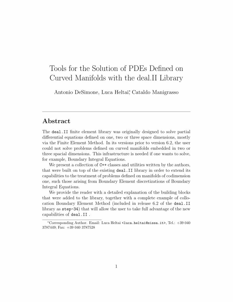
When we work with codimension one objects, there are not only normalsto the faces of the elements as it is usual in the deal.II library, but alsonormals to the cells themselves. It is therefore important to number correctlythe vertices of the cells, so to obtain normals pointing in the desired direction.

The implemented GridIn class respects the orientation of the originalUCD and GMSH files. In these file formats, vertices are ordered either clock-wise, or anticlockwise. We adopted the standard “right handed” orientation,that is, if we face an element whose vertices are oriented anticlockwise, thenormal comes towards us (Figure 1).

While in standard finite element meshes this is not relevant, for boundaryelement methods it is of crucial importance that all elements are oriented ina consistent manner.

An example of mesh in the UCD format (extension .inp) is given by:

8 6 0 0 0

1 -0.577350269 -0.577350269 -0.577350269

2 0.577350269 -0.577350269 -0.577350269

3 -0.577350269 0.577350269 -0.577350269

4 0.577350269 0.577350269 -0.577350269

5 -0.577350269 -0.577350269 0.577350269

6 0.577350269 -0.577350269 0.577350269

7 -0.577350269 0.577350269 0.577350269

5

V2

n

V1

V0

V3

Figure 1: Orientation of the normals with respect to the vertices.

8 0.577350269 0.577350269 0.577350269

1 1 quad 3 4 2 1

2 1 quad 5 6 8 7

3 1 quad 1 2 6 5

4 1 quad 3 7 8 4

5 1 quad 5 7 3 1

6 1 quad 2 4 8 6

which describes the cube inscribed in the sphere of radius 1, with normalsdirected in the outward direction.

Once we create a mesh, it might be of use to perform some local or globalrefinement, in order to improve the accuracy of the computed solution. Whilein standard finite element codes this can be done by adding a vertex in thebarycenter of the cells which are selected for refinement, for codimensionone cells, the manifold that we want to approximate is seldom flat, and itis desirable that new vertices are added that lay on the original manifold,rather than on the approximated one.

To this end, the deal.II library provides a very similar feature for theboundary of finite element meshes in the class Boundary<dim>.

Whenever a cell at the boundary is refined, it is necessary to introduce atleast one new vertex on the boundary. In the simplest case, one assumes that

6

the boundary consists of straight line segments between the vertices of theoriginal, coarsest mesh, and the next vertex is simply put into the middle ofthe old ones. This is the default behavior of the Triangulation<dim> class,and is described by the StraightBoundary<dim> class.

On the other hand, if one deals with curved boundaries, this is not theappropriate thing to do. The classes derived from the Boundary<dim> baseclass therefore describe the geometry of a domain. One can then attach anobject of a class derived from this base class to the Triangulation<dim>

object using the Triangulation<dim>::set boundary() function. Severalclasses exist to support the most common geometries.

We modified the behavior of the original Boundary<dim> class, to adaptit also to the cases where the triangulation describes a codimension onemanifold.

Figure 2: Comparison between mesh refinements with and without manifolddescription.

The use is exactly the same as in the standard case:

...

Point<spacedim> p(0,0,0);

// A spherical surface centered in p with radius 1

HyperBallBoundary<dim, spacedim> boundary(p,1);

7

Triangulation<dim, spacedim> tria;

tria.set_boundary(1, boundary);

...

The different results in case we use or we do not use the boundary de-scription can be seen in Figure 2.

2.2 Basis functions and transformations

Once we have imported and approximated the topological domain, the nextstep is to define the degrees of freedom associated with the vector spacedefined on the approximated domain itself. In the deal.II library thisis obtained through the synergic use of the classes DoFHandler<dim> andFiniteElement<dim>.

Finite element classes describe the properties of a finite element space asdefined on the unit cell. This includes, for example, how many degrees offreedom are located at vertices, on lines, or in the interior of cells. In additionto this, finite element classes of course have to provide values and gradientsof individual shape functions at points on the unit cell.

DoFHandler objects are the confluence of triangulations and finite ele-ments: the finite element class describes how many degrees of freedom itneeds per vertex, line, or cell, and the DoFHandler class allocates this spaceso that each vertex, line, or cell of the triangulation has the correct numberof them and it gives them a global numbering.

Just as with triangulation objects, most operations on DoFHandlers isdone by looping over all cells and doing something on each or a subset ofthem. The interfaces of the two classes are therefore rather similar: theyallow to get iterators to the first and last cell (or face, or line, etc.) and offerinformation through these iterators. The information that can be extractedfrom these iterators is the geometric and topological information that canalready be extracted from the triangulation iterators (they are in fact derivedclasses) as well as things like the global numbers of the degrees of freedomon the present cell.

Among the various possibilities offered by the deal.II library, we limitedthe current implementation of the codimension-one modules to the followingspecializations of the FiniteElement<dim,spacedim> class:

• FE Q<dim,spacedim>: continuous tensor product polynomial space ofarbitrary order;

8

• FE DGQ<dim,spacedim>: discontinuous tensor product polynomial spaceof arbitrary order;

• FE DGP<dim,spacedim>: discontinuous polynomial space of arbitraryorder.

The usage of these classes follows very closely the standard deal.II pro-cedures (see, e.g. [2]):

Triangulation<dim,spacedim> tria;

FE_Q<dim,spacedim> fe(1);

DoFHandler<dim,spacedim> dh(tria);

dh.distribute_dofs(fe);

...

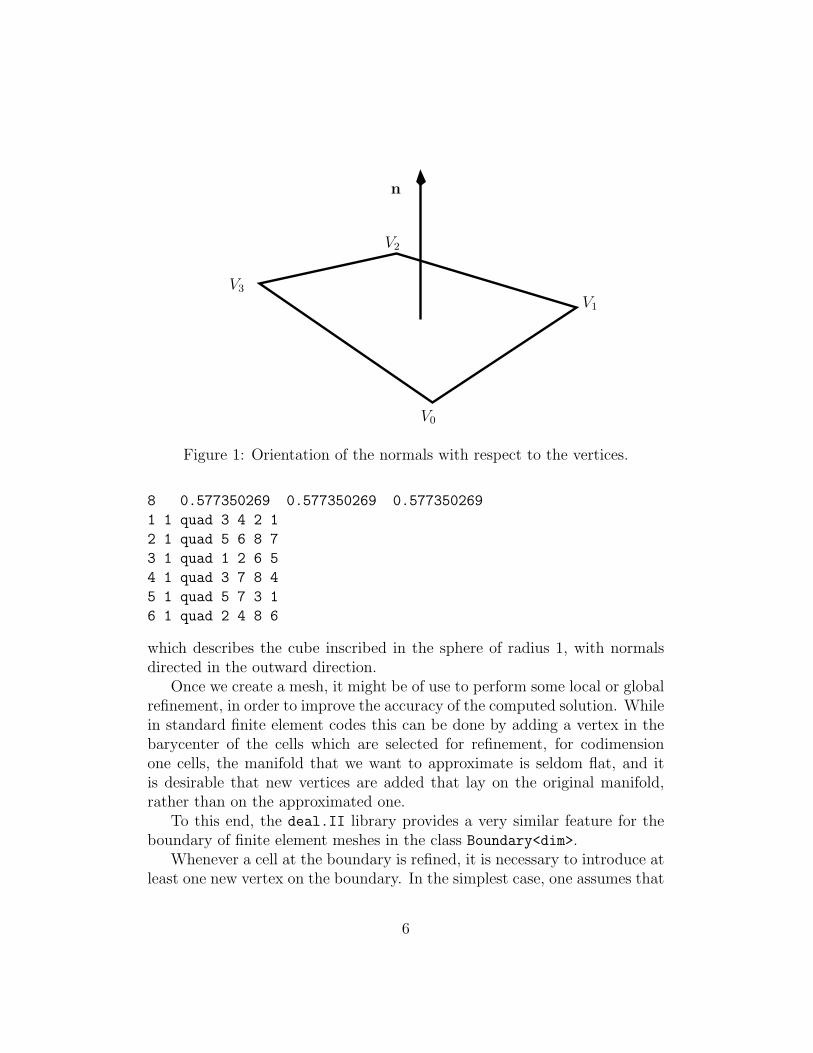
At the end of the above snippet of code, the object dh will contain thedata structures needed to approximate and work with a continuous piecewisebilinear vector space, defined on the manifold approximated by the triangu-lation tria.

In particular we can use the tools provided by the deal.II library todefine a vector of scalar values that uniquely identifies an object of the givenvector space:

...

DoFHandler<dim,spacedim> dh(tria);

...

Vector<double> solution(dh.n_dofs());

...

The vector solution has dimension dh.n dofs(), equal to the numberof degrees of freedom that identifies the vector space dh.

The next step in a finite or boundary element program is that one wouldwant to compute matrix and right hand side entries or other quantities oneach cell of a triangulation, using the shape functions of a finite element andquadrature points defined by a quadrature rule.

To this end, it is necessary to map the shape functions, quadrature points,and quadrature weights from the unit cell to each cell of a triangulation.This is facilitated by the Mapping and derived classes: they describe how tomap points from the unit cell to the real space and back, as well as providegradients of this transformation and Jacobian determinants.

9

For the moment we implemented the MappingQ1<dim,spacedim> andMappingQ1Eulerian<dim,spacedim> class, which extend the functionalityof the original deal.II classes to the codimension one case.

...

QTrapez<dim> quad;

MappingQ1<dim,spacedim> mapping;

typename Triangulation<dim,spacedim>::active_cell_iterator

cell=tria.begin_active(),

endc=tria.end() ;

Point<spacedim> real;

Point<dim> unit;

for(;cell!=endc;++cell)

deallog<<cell<< std::endl;

for(unsigned int q=0; q<quad.n_quadrature_points; ++q)

real = mapping.transform_unit_to_real_cell

(cell, quad.point(q));

std::cout <<quad.point(q)<< " -> " << real << std::endl;

The above snippet of code simply prints the vertices of each cell of thetriangulation, which corresponds to the mapped quadrature points of a trape-zoidal quadrature integration rule in two dimensions from the unit cell (thepoints (0, 0), (1, 0), (0, 1) and (1, 1)) to the real cell.

The next step is to actually take a finite element and evaluate its shapefunctions and their gradients at the points defined by a quadrature formulawhen mapped to the real cell, which is done by the FEValues class.

For example, to compute the total area of a circular or spherical mesh,together with the error in the computation of the outer normals to the cells,one could use the following snippet of code:

...

const QGauss<dim> quadrature(2);

const FE_Q<dim,spacedim> fe (1);

DoFHandler<dim,spacedim> dof_handler (triangulation);

10

K

ξ

η0 1

1

y(η, ξ)

Vi1

Vi0

Vi3

Vi2

Ki

Figure 3: Transformation from reference to real cell.

FEValues<dim,spacedim> fe_values

(dummy_fe, quadrature,

update_JxW_values |

update_cell_normal_vectors |

update_quadrature_points);

dof_handler.distribute_dofs (fe);

double area = 0;

double normals = 0;

typename DoFHandler<dim,spacedim>::active_cell_iterator

cell = dof_handler.begin_active(),

endc = dof_handler.end();

std::vector<Point<spacedim> >

expectedcellnormals(fe_values.n_quadrature_points);

for (; cell!=endc; ++cell)

11

fe_values.reinit (cell);

const std::vector<Point<spacedim> >

& cellnormals =

fe_values.get_cell_normal_vectors();

const std::vector<Point<spacedim> >

& quad_points =

fe_values.get_quadrature_points();

for (unsigned int i=0;

i<fe_values.n_quadrature_points;

++i)

expectedcellnormals[i] =

quad_points[i]/quad_points[i].norm();

area += fe_values.JxW (i);

normals +=

(expectedcellnormals[i]-cellnormals[i]).norm();

;

Notice that in order to compute the outer normals, we introduced a newflag for the FEValues classes, named update cell normal vectors, whichinstructs the FEValues class to compute and store the normals to the cells.

2.3 Interpolation, projection and graphical output

Once we constructed the above tools, the entire machinery is in place thatallows us the use of existent deal.II functions and utilities. An example isthe interpolation and projection of continuous scalar and vector fields on thefinite dimensional spaces defined above.

The deal.II library provided already some utilities to interpolate andproject arbitrary functions on Finite Element spaces. We adapted thesefunctions to be used also with the codimension one versions, such that thefollowing snippet of code can be used, pretty much in the same way that waspreviously available to deal.II users:

...

12

Figure 4: Projection of the cosine function on the surface of a sphere.

Vector<double> projected_one(dof_handler.n_dofs());

Functions::CosineFunction<spacedim> cosine;

QGauss<dim> quad(5);

ConstraintMatrix constraints;

constraints.close();

VectorTools::project

(dof_handler,

constraints,

quad,

cosine,

projected_one);

13

VectorTools::interpolate

(dof_handler,

constant,

interpolated_one);

The result of the given example can be seen in Figure 4, which was realizedusing the class DataOut. Again, this class was modified to accept the newcodimension one objects without changing the user interface:

DataOut<dim, DoFHandler<dim,spacedim> > dataout;

dataout.attach_dof_handler(dof_handler);

dataout.add_data_vector(projected_one, "projection");

dataout.build_patches();

std::ofstream file("output.vtk");

dataout.write_vtk(file);

3 A complete example

We wrote a complete example to show in great details the usage of all theadded tools in a concrete case ([5]) which has been included in version 6.2of the deal.II library. Here we describe some details of its implementationwhich allows one to solve the problem of irrotational fluid flowing around acircular or a spherical obstacle in two or three spacial dimensions respectively.

3.1 Mathematical overview

The motion of an inviscid fluid past a body at rest is usually modeled by theEuler equations of fluid dynamics:

∂∂t

v + (v · ∇)v = −1ρ∇p+ g in Rn\Ω

∇ · v = 0 in Rn\Ω , (1)

where the fluid density ρ and the acceleration g due to external forces aregiven, while the velocity v and the pressure p are the unknowns. Here Ω is aclosed bounded region representing the body around which the fluid movesand we assume that the boundary Γ = ∂Ω is sufficiently smooth.

14

Uniqueness of the solution is ensured by the following boundary condi-tions

n · v = 0 on ∂Ω

v = v∞ when |x| → ∞,(2)

which mean that the body is not permeable, and that the fluid is assumedin uniform motion at infinity.

Equations (1) can be derived from Navier-Stokes equations assuming thatthe effects due to viscosity are negligible compared to those due to the pres-sure gradient and to the external forces.

We will concentrate only on the stationary solutions to problem (1).These solutions are typically used to understand the behavior of the given(possibly complex) geometry when a fluid moves around it or, equivalently,when a prescribed motion, e.g., a translation, is enforced on the body. Thismodel can describe for example the motion of air past an airplane wing, or,with some trivial modifications, the motion of air or water past a propellerrotating at constant speed.

For both stationary and non stationary flow, the solution is sought bysolving firstly for the velocity in the second equation and then by substitut-ing in the first equation in order to find the pressure. It is convenient todecompose the velocity of the fluid in a uniform background field v∞ and ina perturbation field vp which is due to the presence of the body Ω

∇ · v = ∇ · (v∞ + vp) = ∇ · vp = 0.

If we assume that the fluid is irrotational, i.e., ∇ × v = 0 in Rn\Ω, wecan represent the velocity, and consequently also the perturbation velocity,as the gradient of a scalar function:

vp = ∇φ,

which implies that the second of equations (1) above can be rewritten asLaplace equation for the unknown φ with Neumann boundary conditions onthe boundary ∂Ω

∆φ = 0 in Ω

n · ∇φ = −n · v∞ on ∂Ω (3)

φ = φ∞ when |x| → ∞, (4)

15

where the last condition ensures unicity. The conservation of momentumequation (the first of equations (1)) reduces to Bernoulli’s equation thatexpresses the pressure p as a function of the potential φ:

p

ρ+

1

2|∇φ|2 = 0 ∈ Ω.

Notice that, by assuming that the flow is irrotational, we completelydecoupled the conservation of momentum from the conservation of mass,and the two problems can be solved one after the other. For what follows,we will only be interested in solving for the unknown potential φ, since thepressure can be easily recovered by postprocessing the solution φ.

Figure 5: Three dimensional irrotational flow cannot generate lift.

The irrotationality assumption is not without consequences, since it af-fects in a significant way the properties of the solutions. The Kutta-Jukowskitheorem (see, e.g., chapter 4 of [1]), states that a flux can generate lift onlyif the circulation

∮C

v · ds on any closed curve C around the body is differentfrom zero. Using Stoke’s theorem this implies that∮

C

v · ds =

∫S

∇× v dx

16

where S is any surface with C as boundary.In two dimensions the integral above vanishes if S does not contain Ω,

but can be different from zero otherwise, which implies that Euler equationscan describe a lifting flux.

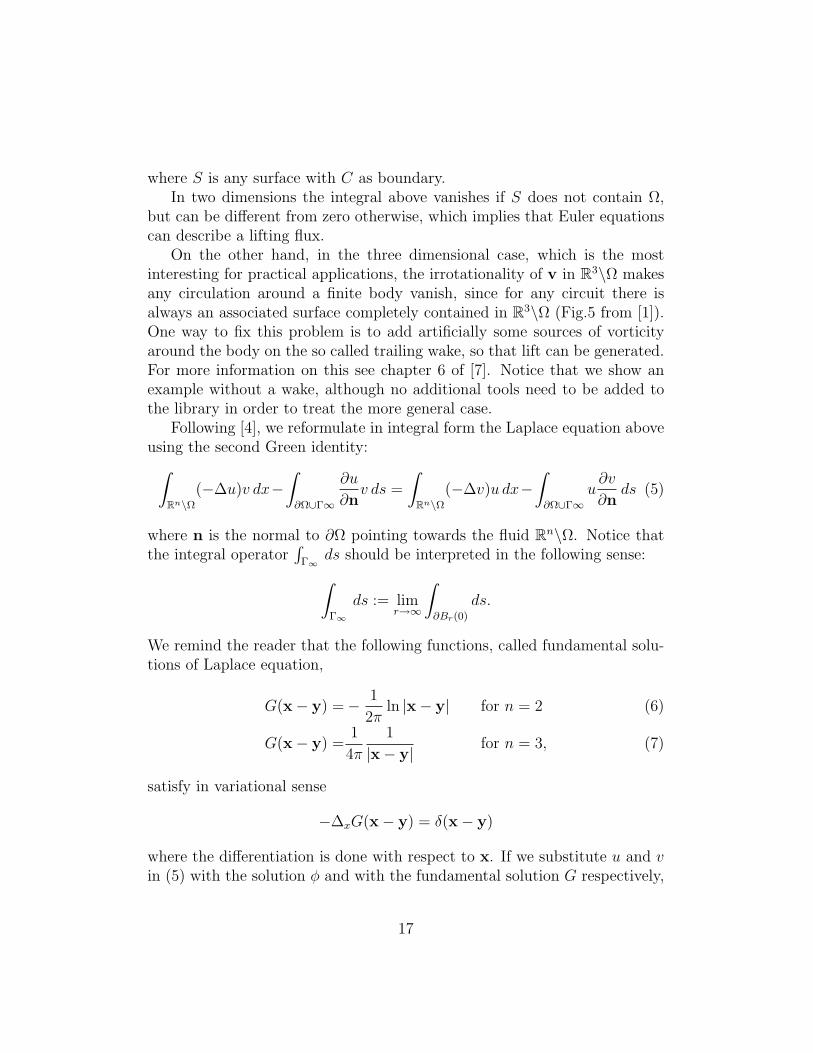
On the other hand, in the three dimensional case, which is the mostinteresting for practical applications, the irrotationality of v in R3\Ω makesany circulation around a finite body vanish, since for any circuit there isalways an associated surface completely contained in R3\Ω (Fig.5 from [1]).One way to fix this problem is to add artificially some sources of vorticityaround the body on the so called trailing wake, so that lift can be generated.For more information on this see chapter 6 of [7]. Notice that we show anexample without a wake, although no additional tools need to be added tothe library in order to treat the more general case.

Following [4], we reformulate in integral form the Laplace equation aboveusing the second Green identity:∫

Rn\Ω(−∆u)v dx−

∫∂Ω∪Γ∞

∂u

∂nv ds =

∫Rn\Ω

(−∆v)u dx−∫∂Ω∪Γ∞

u∂v

∂nds (5)

where n is the normal to ∂Ω pointing towards the fluid Rn\Ω. Notice thatthe integral operator

∫Γ∞

ds should be interpreted in the following sense:∫Γ∞

ds := limr→∞

∫∂Br(0)

ds.

We remind the reader that the following functions, called fundamental solu-tions of Laplace equation,

G(x− y) =− 1

2πln |x− y| for n = 2 (6)

G(x− y) =1

4π

1

|x− y|for n = 3, (7)

satisfy in variational sense

−∆xG(x− y) = δ(x− y)

where the differentiation is done with respect to x. If we substitute u and vin (5) with the solution φ and with the fundamental solution G respectively,

17

we obtain for all x ∈ Rn\Ω

φ(x) = −∫∂Ω∪Γ∞

G(x− y)∂φ

∂ny(y) dsy +

∫∂Ω∪Γ∞

∂G(x− y)

∂nyφ(y) dsy

= φ∞ −∫∂Ω

G(x− y)∂φ

∂ny(y) dsy +

∫∂Ω

∂G(x− y)

∂nyφ(y) dsy. (8)

In the above was used the fact that, since limx→∞ φ(x) = φ∞ ∈ R, one hasto consider only the term∫

Γ∞

∂G(x− y)

∂nyφ(y) dsy = − lim

r→∞

∫∂Br(0)

r

r∇G(x− y)φ∞ dsy = φ∞.

Equation (8) can be rewritten in a more compact form using the SingleLayer Potential (SLP) and the Double Layer Potential (DLP) operators:

φ(x) = φ∞ −(S∂φ

∂ny

)(x) + (Dφ)(x) for all x ∈ Rn\Ω. (9)

It can be shown that (3) and (9) are equivalent [4]. Notice also that thelast equation allows one to calculate φ in any point of the domain once itsexpression on the boundary ∂Ω is known.

If we impose the boundary conditions (2) we obtain:

n · (v∞ + vp) = 0 ⇒ n · vp = −n · v∞ ⇒ ∂φ

∂n= −n · v∞.

Moreover (see, for example, [8]) if we take the limit for x tending to ∂Ω inequation (9) we can reduce it to an expression on the boundary only:

α(x)φ(x) = φ∞ + (S[n · v∞]) (x) + (Dφ)(x) for all x ∈ ∂Ω, (10)

which is the integral formulation we were looking for. The quantity α(x)is the fraction of angle or of solid angle by which the point x sees the fluidRn\Ω. In particular, at points x where the boundary ∂Ω is differentiablewe have α(x) = 1/2, but the value may be different at points where theboundary has a corner or an edge.

18

Substituting the explicit expressions of SLP and DLP we can rewriteequation (10) as:

α(x)φ(x) =φ∞ −1

2π

∫∂Ω

ln |x− y|n · v∞ dsy +1

2π

∫∂Ω

(x− y) · ny|x− y|2

φ(y) dsy

(11)

α(x)φ(x) =φ∞ +1

4π

∫∂Ω

1

|x− y|n · v∞ dsy +

1

4π

∫∂Ω

(x− y) · ny|x− y|3

φ(y) dsy

(12)

for two dimensional and for three dimensional flows respectively.Since the constant function φ(x) = φ∞ is a solution of the Laplace equa-

tion with zero Neumann data, the following expression

α(x) := 1− 1

2(n− 1)π

∫∂Ω

(y − x) · ny|y − x|n

φ(y) dsy = 1 +

∫∂Ω

∂G(y − x)

∂nydsy,

can be used to derive explicitly the values of α(x) on ∂Ω.

3.2 Numerical approximation

Numerical approximations of boundary integral equations are commonly re-ferred to as the Boundary Element Method or Panel Method (the latter ex-pression being used mostly in the computational fluid dynamics community[6]). This naming convention derives from the use of quadrilateral meshesfor the discretization of the computational domain in panels.

The goal of the following test problem is to solve the integral formulationof the Laplace equation described in the previous section, using a circle anda sphere respectively in two and three space dimensions. To this end, letTh =

⋃Mi Ki be a partition of the manifold Γ = ∂Ω into M line segments if

n = 2, or M quadrilaterals if n = 3. We will call each individual Ki elementor cell, independently of the dimension of the space and we require that thepartition, more frequently referred to as triangulation, be regular in the senseexplained in [10]. We define the finite dimensional space Vh as

Vh := v ∈ C0(Γ) s.t. v|Ki∈ Q1(K),∀K ∈ Th

where Q1(K) indicates the space of polynomials of maximum degree 1 ineach variable on the domain K. An element φh of Vh is uniquely determined

19

by the vector φ of its coefficients φi, that is:

φh(x) :=N∑i=1

φiψi(x), φ := φi,

where ψi is the set of basis functions that has cardinality N = dimVh. Thereader is reminded that each of these functions is associated to a vertex ofthe triangulation, so that it takes the value 1 on one vertex and vanishes onall the others:

ψi(xj) = δij. (13)

By far, the most common approximation of boundary integral equationsin the engineering community is by use of the collocation boundary elementmethod. This method requires that the boundary integral equation be sat-isfied at a number of collocation points which is equal to the number ofunknowns of the system, namely the N coefficients that identify the solutionφh. The choice of these points is a delicate matter, but let us assume for themoment that their are known, and call them xi with i = 0...N .

If we consider equation (10), we obtain the following problem. Given thedatum v∞, find a function φh in Vh such that the N equations

α(xi)φh(xi)−∫

Γy

∂G(y − xi)

∂nyφh(y) dsy =

∫Γy

G(y − xi) ny · v∞ dsy,

are satisfied, where we have set the arbitrary constant φ∞ in (10) to zero.The problem can then be written as the following linear system:

(A + N)φ = b

where

Aij = α(xi)ψj(xi) = 1 +

∫Γ

∂G(y − xi)

∂nydsyψj(xi)

Nij = −∫

Γ

∂G(y − xi)

∂nyψj(y) dsy

bi =

∫Γ

G(y − xi) ny · v∞dsy.

From a linear algebra point of view, the best possible choice of the collocationpoints is the one that renders the matrix A+N the most diagonally dominant.A natural choice is then to select the xi collocation points to be the vertices

20

associated to the nodal basis functions ψi(x). As a consequence of (13), thematrix A is diagonal with entries

Aii = 1 +

∫Γ

∂G(y − xi)

∂nydsy = 1−

∑j

Nij

where we have used that∑

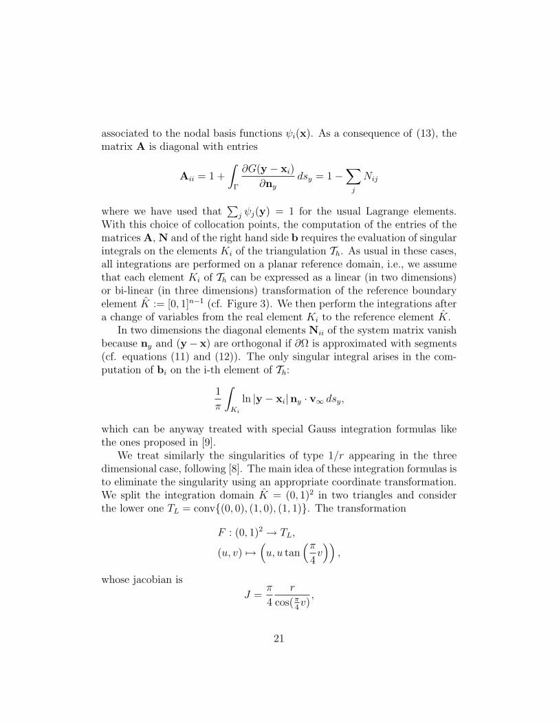
j ψj(y) = 1 for the usual Lagrange elements.With this choice of collocation points, the computation of the entries of thematrices A, N and of the right hand side b requires the evaluation of singularintegrals on the elements Ki of the triangulation Th. As usual in these cases,all integrations are performed on a planar reference domain, i.e., we assumethat each element Ki of Th can be expressed as a linear (in two dimensions)or bi-linear (in three dimensions) transformation of the reference boundaryelement K := [0, 1]n−1 (cf. Figure 3). We then perform the integrations aftera change of variables from the real element Ki to the reference element K.

In two dimensions the diagonal elements Nii of the system matrix vanishbecause ny and (y− x) are orthogonal if ∂Ω is approximated with segments(cf. equations (11) and (12)). The only singular integral arises in the com-putation of bi on the i-th element of Th:

1

π

∫Ki

ln |y − xi|ny · v∞ dsy,

which can be anyway treated with special Gauss integration formulas likethe ones proposed in [9].

We treat similarly the singularities of type 1/r appearing in the threedimensional case, following [8]. The main idea of these integration formulas isto eliminate the singularity using an appropriate coordinate transformation.We split the integration domain K = (0, 1)2 in two triangles and considerthe lower one TL = conv(0, 0), (1, 0), (1, 1). The transformation

F : (0, 1)2 → TL,

(u, v) 7→(u, u tan

(π4v))

,

whose jacobian is

J =π

4

r

cos(π4v),

21

TL

x

y v

u

K

Figure 6: Coordinate transformation for the treatment of singularities in thethree dimensional case.

introduces a term proportional to r into the integral. This term cancels outthe singularity in the integrand and we can use the ordinary Gauss integrationformulas (Figure 6). The upper triangle in the reference element K can bethen treated analogously.

The resulting matrix A + N is full. Depending on its size, it might beconvenient to use a direct solver or an iterative one. For the purpose of thisexample code, we chose to use only an iterative solver, without providing anypreconditioner.

If this were an industrial project rather than a demonstration of the newfunctionalities added to deal.II , the need for precision would soon requirea large number of panels and the solution of a linear system of the typedescribed above with a large number of unknowns would not be feasible.In this case more sophisticated techniques are available that allow one notto store full matrices by neglecting higher order terms due to panels faraway from each other. In the literature on boundary element methods a

22

plethory of these methods have been developed, leading to a significantlysparser representation of these matrices that also facilitates rapid evaluationof vector-matrix products ([10], [8]).

3.3 Implementation

We will now discuss the actual implementation of the problem, an exampleof which is the tutorial step-34 in the deal.II library [5]. In order tounderstand this example, the reader is recommended to practice with thedeal.II framework using the large set of tutorials that are distributed withthe library. We suggest to read at least the first five tutorials to get familiarwith the basic steps in the implementation of a problem.

The main structure of the program is implemented in the BEMProblem

class. This structure should be already familiar to deal.II users, as well asto any Finite Element code programmers, as it is almost self explanatory:

template <int dim>

class BEMProblem

public:

BEMProblem();

void run();

private:

void read_parameters (const std::string &filename);

void read_domain();

void refine_and_resize();

void assemble_system();

void solve_system();

void compute_errors(const unsigned int cycle);

23

void compute_exterior_solution();

void output_results(const unsigned int cycle);

The only really new function that we find here is the assembly routine.We wrote this function in the most possible general way, in order to allowfor easy generalization to higher order methods and to different fundamentalsolutions (e.g., Stokes or Maxwell). The most noticeable difference fromFEM codes is the fact that the final matrix is full, and that we have a nestedloop inside the usual loop on cells that visits all the points associated to thedegrees of freedom. Moreover, when the point lies inside the cell which isbeing visited, the integrand becomes singular and needs a special treatment.The practical consequence is that we have two sets of quadrature formulas,finite element values and temporary data, one for standard integration andone for the singular integration.

We opted for an iterative solver in the function solve_system(). Thematrix that we assemble is full and not symmetric, and we chose the unpre-conditioned GMRES method. The options for the iterative solver, such asthe tolerance and the maximum number of iterations are selected throughthe parameter file (cf. the function read_parameters()).

Once we obtained the solution, we compute the L2 error of the po-tential as well as the L∞ error of the approximation of the solid angle incompute_errors(). The mesh we are using is an approximation of a smoothcurve or surface, therefore the computed diagonal matrix of fraction of anglesor solid angles α(x) should contain entries that approximate the exact value1/2.

Once a solution on the codimension one domain is obtained, we would liketo extend it to the rest of the external space Rn\Ω. This is done by performingthe convolution of the solution with the kernel in the compute_exterior_solution()function, following equation (8). The velocity field can then be easily ob-tained computing the gradient of the potential. All the results are plottedby the function output_results().

The objects that will be shared by the functions of the class are thendeclared specifying the optional argument that indicates the dimension ofthe space the body is embedded in.

Triangulation<dim-1,dim> tria;

24

FE_Q<dim-1,dim> fe;

DoFHandler<dim-1,dim> dh;

FullMatrix<double> system_matrix;

Vector<double> system_rhs;

Vector<double> phi;

Vector<double> alpha;

ConvergenceTable convergence_table;

Functions::ParsedFunction<dim> wind;

Functions::ParsedFunction<dim> exact_solution;

std_cxx1x::shared_ptr<Quadrature<dim-1> > quadrature;

unsigned int singular_quadrature_order;

SolverControl solver_control;

unsigned int n_cycles;

unsigned int external_refinement;

bool run_in_this_dimension;

bool extend_solution;

;

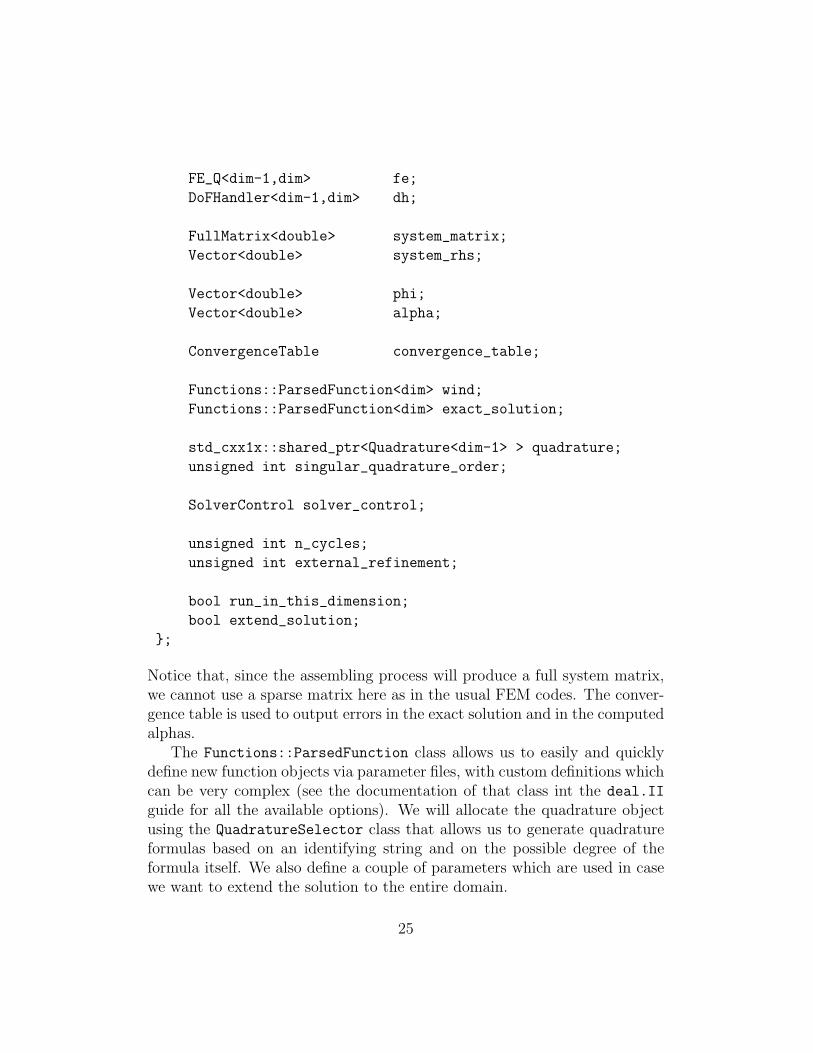
Notice that, since the assembling process will produce a full system matrix,we cannot use a sparse matrix here as in the usual FEM codes. The conver-gence table is used to output errors in the exact solution and in the computedalphas.

The Functions::ParsedFunction class allows us to easily and quicklydefine new function objects via parameter files, with custom definitions whichcan be very complex (see the documentation of that class int the deal.II

guide for all the available options). We will allocate the quadrature objectusing the QuadratureSelector class that allows us to generate quadratureformulas based on an identifying string and on the possible degree of theformula itself. We also define a couple of parameters which are used in casewe want to extend the solution to the entire domain.

25

In the following we will give an outline of the most important parts ofthe program (we refer the reader to [5] for the complete code and for furtherexplanations).

3.3.1 Assembling the system matrix

The main difficulty encountered in this routine is the treatment of the sin-gular integrals. At the beginning of this function, we create the singularquadrature formulas for the three dimensional problem. Here we define avector of four such quadratures (one per each vertex of a cell) that will beused later on.

template <int dim>

void BEMProblem<dim>::assemble_system()

std::vector<QGaussOneOverR<2> > sing_quadratures_3d;

for(unsigned int i=0; i<4; ++i)

sing_quadratures_3d.push_back

(QGaussOneOverR<2>(singular_quadrature_order, i, true));

Next, we initialize a FEValues object with the quadrature formula for theintegration of the kernel in non singular cells. This quadrature is selectedwith the parameter file, and needs to be quite precise, since the functions weare integrating are not polynomial functions.

FEValues<dim-1,dim> fe_v(fe, *quadrature,

update_values |

update_cell_normal_vectors |

update_quadrature_points |

update_JxW_values);

const unsigned int n_q_points = fe_v.n_quadrature_points;

std::vector<unsigned int> local_dof_indices(fe.dofs_per_cell);

std::vector<Vector<double> > cell_wind(n_q_points, Vector<double>(dim) );

double normal_wind;

Unlike in finite element methods, if we use collocation BEM, then in eachassembly loop we only assemble the information that refers to the coupling

26

between one degree of freedom (the degree associated with vertex i) and thecurrent cell.

We can start the integration loop over all cells, where we first initializethe FEValues object and get the values of vp at the quadrature points:

typename DoFHandler<dim-1,dim>::active_cell_iterator

cell = dh.begin_active(),

endc = dh.end();

for(cell = dh.begin_active(); cell != endc; ++cell)

fe_v.reinit(cell);

cell->get_dof_indices(local_dof_indices);

const std::vector<Point<dim> > &q_points =

fe_v.get_quadrature_points();

const std::vector<Point<dim> > &normals =

fe_v.get_cell_normal_vectors();

wind.vector_value_list(q_points, cell_wind);

We then compute the integral over the current cell for all degrees of freedom(note that this includes also degrees of freedom not located on the currentcell, a deviation from the usual finite element integrals). The integral thatwe need to perform is singular if one of the local degrees of freedom is thesame as the support point i. If the index i is not one of the local degreesof freedom, we simply have to add the single layer terms to the right handside, and the double layer terms to the matrix:

if(is_singular == false)

for(unsigned int q=0; q<n_q_points; ++q)

normal_wind = 0;

for(unsigned int d=0; d<dim; ++d)

normal_wind += normals[q][d]*cell_wind[q](d);

const Point<dim> R = q_points[q] - support_points[i];

system_rhs(i) += ( LaplaceKernel::single_layer(R)*

27

normal_wind*

fe_v.JxW(q) );

for(unsigned int j=0; j<fe.dofs_per_cell; ++j)

local_matrix_row_i(j) -= ( ( LaplaceKernel::double_layer(R)*

normals[q] )*

fe_v.shape_value(j,q)*

fe_v.JxW(q) );

else

Now we treat the more delicate case. In this case both the single and thedouble layer potential are singular, and they require special treatment asdescribed earlier. In one dimension this process does not result only in afactor appearing as a constant factor on the entire integral, but also on anadditional integral alltogether that needs to be evaluated:∫ 1

0

f(x) ln(x/α)dx =

∫ 1

0

f(x) ln(x)dx−∫ 1

0

f(x) ln(α)dx.

This process is taken care of by the constructor of the QGaussLogR class,which adds additional quadrature points and weights to take into considera-tion also the second part of the integral.

Putting all this into a dimension independent framework requires a littletrick. The problem is that, depending on the dimension, we would like toeither assign a QGaussLogR<1> or a QGaussOneOverR<2> to aQuadrature<dim-1>. C++ does not allow this right away, and neither is astatic_cast possible but we are allowed to do a dynamic_cast.

const Quadrature<dim-1> *

singular_quadrature

= (dim == 2?

dynamic_cast<Quadrature<dim-1>*>(

new QGaussLogR<1>(singular_quadrature_order,

Point<1>((double)singular_index),

1./cell->measure(), true))

:

(dim == 3?

dynamic_cast<Quadrature<dim-1>*>(

28

&sing_quadratures_3d[singular_index])

:0));

Assert(singular_quadrature, ExcInternalError());

...

for(unsigned int q=0; q<singular_quadrature->size(); ++q)

const Point<dim> R = singular_q_points[q] - support_points[i];

double normal_wind = 0;

for(unsigned int d=0; d<dim; ++d)

normal_wind += (singular_cell_wind[q](d)*

singular_normals[q][d]);

system_rhs(i) += ( LaplaceKernel::single_layer(R) *

normal_wind*

fe_v_singular.JxW(q) );

for(unsigned int j=0; j<fe.dofs_per_cell; ++j)

local_matrix_row_i(j) -= (( LaplaceKernel::double_layer(R) *

singular_normals[q])*

fe_v_singular.shape_value(j,q)*

fe_v_singular.JxW(q) );

if(dim==2)

delete singular_quadrature;

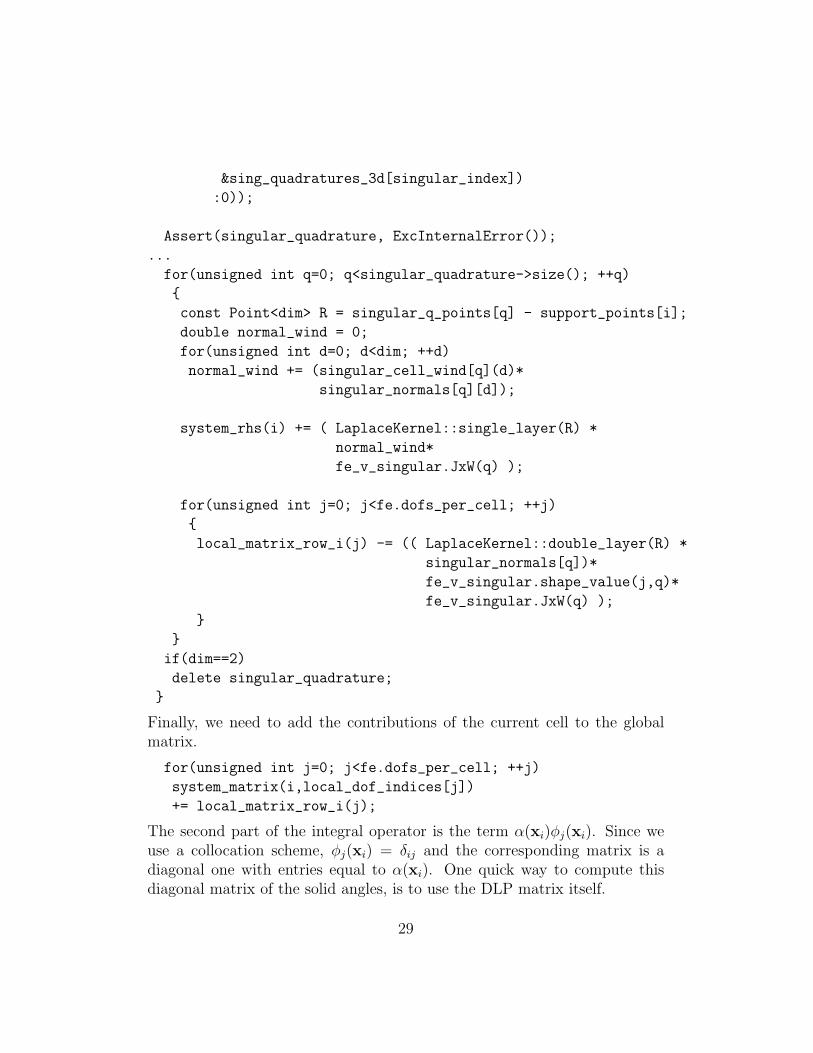
Finally, we need to add the contributions of the current cell to the globalmatrix.

for(unsigned int j=0; j<fe.dofs_per_cell; ++j)

system_matrix(i,local_dof_indices[j])

+= local_matrix_row_i(j);

The second part of the integral operator is the term α(xi)φj(xi). Since weuse a collocation scheme, φj(xi) = δij and the corresponding matrix is adiagonal one with entries equal to α(xi). One quick way to compute thisdiagonal matrix of the solid angles, is to use the DLP matrix itself.

29

Vector<double> ones(dh.n_dofs());

ones.add(-1.);

system_matrix.vmult(alpha, ones);

alpha.add(1);

for(unsigned int i = 0; i<dh.n_dofs(); ++i)

system_matrix(i,i) += alpha(i);

3.3.2 Extending the solution

With this function we compute finally the value of the potential φ in the exte-rior domain Rn\Ω, considering that our original problem consist in knowingthe velocity field in the fluid.

To this end, we extrapolate the actual solution inside the box [−2, 2]dim

using the convolution with the fundamental solution. The reconstruction ofthe solution in the entire space is done on a continuous finite element grid ofdimension dim.

template <int dim>

void BEMProblem<dim>::compute_exterior_solution()

Triangulation<dim> external_tria;

GridGenerator::hyper_cube(external_tria, -2, 2);

FE_Q<dim> external_fe(1);

DoFHandler<dim> external_dh (external_tria);

Vector<double> external_phi;

...

typename DoFHandler<dim-1,dim>::active_cell_iterator

cell = dh.begin_active(),

endc = dh.end();

FEValues<dim-1,dim> fe_v(fe, *quadrature,

update_values |

update_cell_normal_vectors |

update_quadrature_points |

update_JxW_values);

30

...

typename DoFHandler<dim>::active_cell_iterator

...

std::vector<Point<dim> > external_support_points

(external_dh.n_dofs());

DoFTools::map_dofs_to_support_points<dim>

( StaticMappingQ1<dim>::mapping,

external_dh, external_support_points);

for(cell = dh.begin_active(); cell != endc; ++cell)

...

for(unsigned int i=0; i<external_dh.n_dofs(); ++i)

for(unsigned int q=0; q<n_q_points; ++q)

const Point<dim> R =

q_points[q] - external_support_points[i];

external_phi(i) +=

( ( LaplaceKernel::single_layer(R) *

normal_wind[q]

+

(LaplaceKernel::double_layer(R) *

normals[q] ) *

local_phi[q] ) *

fe_v.JxW(q) );

...

3.3.3 Numerical results and solution plotsr

As we can see from the convergence table in two dimensions, if we choosequadrature formulas which are accurate enough, then the error we obtainfor α(x) should be exactly the inverse of the number of elements. The ap-proximation of the circle with N segments of equal size generates a regular

31

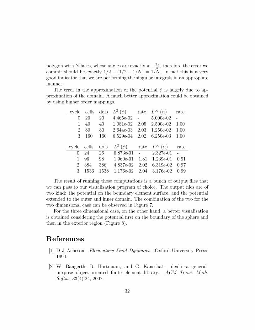
polygon with N faces, whose angles are exactly π− 2πN

, therefore the error wecommit should be exactly 1/2 − (1/2 − 1/N) = 1/N . In fact this is a verygood indicator that we are performing the singular integrals in an appropiatemanner.

The error in the approximation of the potential φ is largely due to ap-proximation of the domain. A much better approximation could be obtainedby using higher order mappings.

cycle cells dofs L2 (φ) rate L∞ (α) rate0 20 20 4.465e-02 - 5.000e-02 -1 40 40 1.081e-02 2.05 2.500e-02 1.002 80 80 2.644e-03 2.03 1.250e-02 1.003 160 160 6.529e-04 2.02 6.250e-03 1.00

cycle cells dofs L2 (φ) rate L∞ (α) rate0 24 26 6.873e-01 - 2.327e-01 -1 96 98 1.960e-01 1.81 1.239e-01 0.912 384 386 4.837e-02 2.02 6.319e-02 0.973 1536 1538 1.176e-02 2.04 3.176e-02 0.99

The result of running these computations is a bunch of output files thatwe can pass to our visualization program of choice. The output files are oftwo kind: the potential on the boundary element surface, and the potentialextended to the outer and inner domain. The combination of the two for thetwo dimensional case can be observed in Figure 7.

For the three dimensional case, on the other hand, a better visualisationis obtained considering the potential first on the boundary of the sphere andthen in the exterior region (Figure 8).

References

[1] D J Acheson. Elementary Fluid Dynamics. Oxford University Press,1990.

[2] W. Bangerth, R. Hartmann, and G. Kanschat. deal.ii–a general-purpose object-oriented finite element library. ACM Trans. Math.Softw., 33(4):24, 2007.

32

Figure 7: Potential φ on the boundary of the circle and in the exterior region.

[3] W Bangerth, Hartmann R, and Kanschat G. deal.II Technical Reference. http://www.dealii.org, 2009.

[4] L. Banjai. Boundary Element Methods. Course notes, 2007.

[5] L. Heltai. Step 34, deal.II tutorial.http://www.dealii.org/developer/doxygen/deal.II/step 34.html, 2009.

[6] J L Hess. Panel Methods in Computational Fluid Dynamics. AnnualReviews in Fluid Mechanics, 22(1):255–274, 1990.

[7] C. Marchioro and M. Pulvirenti. Mathematical Theory of IncompressibleNonviscous Fluids. Springer, 1994.

[8] Andrea Mola. Models for Olympic Rowing Boats. PhD thesis, MOX -Politecnico di Milano, 2009.

33

Figure 8: Potential φ on the boundary of the sphere and in the exteriorregion.

[9] William Press, Saul Teukolsky, William Vetterling, and Brian Flannery.Numerical Recipes in C. Cambridge University Press, Cambridge, UK,2nd edition, 1992.

[10] S. Sauter and C. Schwab. Randelementmethoden. Teubner, 2004.

34