Embed Size (px)
Citation preview
Forschungsinstitut zur Zukunft der ArbeitInstitute for the Study of Labor
DI
SC
US
SI
ON
P
AP
ER
S
ER
IE
S
Top Incomes and Human Well-beingaround the World
IZA DP No. 9677
January 2016
Richard V. BurkhauserJan-Emmanuel De NeveNattavudh Powdthavee
Top Incomes and Human Well-being around the World
Richard V. Burkhauser Cornell University,
University of Melbourne and IZA
Jan-Emmanuel De Neve
University of Oxford
Nattavudh Powdthavee
London School of Economics, University of Melbourne and IZA
Discussion Paper No. 9677 January 2016
IZA
P.O. Box 7240 53072 Bonn
Germany
Phone: +49-228-3894-0 Fax: +49-228-3894-180
E-mail: [email protected]
Any opinions expressed here are those of the author(s) and not those of IZA. Research published in this series may include views on policy, but the institute itself takes no institutional policy positions. The IZA research network is committed to the IZA Guiding Principles of Research Integrity. The Institute for the Study of Labor (IZA) in Bonn is a local and virtual international research center and a place of communication between science, politics and business. IZA is an independent nonprofit organization supported by Deutsche Post Foundation. The center is associated with the University of Bonn and offers a stimulating research environment through its international network, workshops and conferences, data service, project support, research visits and doctoral program. IZA engages in (i) original and internationally competitive research in all fields of labor economics, (ii) development of policy concepts, and (iii) dissemination of research results and concepts to the interested public. IZA Discussion Papers often represent preliminary work and are circulated to encourage discussion. Citation of such a paper should account for its provisional character. A revised version may be available directly from the author.
IZA Discussion Paper No. 9677 January 2016
ABSTRACT
Top Incomes and Human Well-being Around the World* The share of income held by the top 1 percent in many countries around the world has been rising persistently over the last 30 years. But we continue to know little about how the rising top income shares affect human well-being. This study combines the latest data to examine the relationship between top income share and different dimensions of subjective well-being. We find top income shares to be significantly correlated with lower life evaluation and higher levels of negative emotional well-being, but not positive emotional well-being. The results are robust to household income, individual’s socio-economic status, and macroeconomic environment controls. JEL Classification: D63, I3 Keywords: top income, life evaluation, well-being, income inequality,
World Top Income Database, Gallup World Poll Corresponding author: Richard V. Burkhauser Department of Policy Analysis and Management Cornell University 259 MVR Hall Ithaca, NY 14853 USA E-mail: [email protected]
* The authors are grateful to Andrew Clark, Paul Frijters, Carol Graham, Richard Layard, Andrew Oswald and participants at the Well-Being seminar at London School of Economics for their many useful comments. R.V.B. and N.P. designed research; J-E.D.N. provided access to the GWP data; N.P. analyzed data; R.V.B., J-E.D.N. and N.P. wrote the paper. The Gallup World Poll data used in this research belongs to the Gallup Organization. The data are made available by the Gallup Organization for a fee. For more information, see: http://www.gallup.com/services/170945/world-poll.aspx. The data is made available for free to researchers who obtain “Research Advisor” status with the Gallup Organization. The British Household Panel Survey (BHPS) data used in this paper were made available through the UK Data Archive. The data were originally collected by the ESRC Longitudinal Studies Centre (ULSC), together with the Institute for Social and Economic Research (ISER) at the University of Essex. The World Top Income Database is made available from the Paris School of Economics’ website at http://topincomes.parisschoolofeconomics.eu.
3
There is a growing concern within the social science community over the economic and
social implications of the persistent rise in top income shares in the United States and in most
other rich countries around the world over the last three decades. Although much of the recent
economic research on the topic of income inequality has focused on the identification of the
“Top 1 percent”1 and their dynamics over a long period of time (Atkinson, Piketty, & Saez,
2011; Burkhauser et al., 2012; Piketty & Saez 2014), we continue to know very little about the
possible links between the rising share of national income accruing to the top percentile and
aggregated well-being. Does income inequality at the very top matter to the average life
evaluation when household income is held constant? What about the emotional quality of an
individual’s everyday experiences, that is, the frequency and intensity of experiences of joy,
sadness, anger, and affection that make one’s life pleasant or unpleasant? In other words, do the
majority of people even care about the rising income shares of a small number of individuals in
their country? Although these are difficult questions, they are important to our understanding of
the welfare implications of rising top income shares around the world.
Our paper is the first to empirically link the rising share of national income accruing to
the top percentile to aggregated well-being. Using data from the Gallup World Poll, we first
present econometric evidence showing that top income shares strongly predict lower individual
life evaluation and higher negative emotional daily experiences, but in most cases are not
significantly correlated with positive emotional daily experiences. The magnitude of the negative
1The top income literature is based on income tax records. Hence it focuses on the share of taxable income held by
the top 1 percent of tax unit where a tax unit can be an individual or a family. The survey literature primarily focuses
on households. See Burkhauser et al. (2012) for a discussion of this distinction in the context of the top income
literature.
4
top income shares coefficient in the life evaluation equation is quantitatively important as well as
statistically significant. Holding other things constant—including log of GDP per capita, own
income, and the income of a reference group—a 1% increase in the share of taxable income held
by the top 1 percent has an equivalent impact on life evaluation as a 1.4% increase in the
country-level unemployment rate. In a later analysis, we are able to replicate our earlier results
using the British Household Panel Study (BHPS), a long-running household panel that contains
life evaluation information as well as household income data. Overall, our results indicate that
top income shares are one of the most statistically important and sizeable country-level
determinants of international differences in how people around the world evaluate their lives.
I. Background
In recent years there has been an accumulation of empirical evidence suggesting that
individuals are less satisfied with life when income inequality is high (e.g., Blanchflower and
Oswald, 2003; Alesina et al., 2004; Schwarze and Harper, 2007; Ferrer-i-Carbonell and Ramos,
2009; Verme, 2011; Oishi and Kesebir, forthcoming)2. Yet, a more careful look into the literature
suggests that the relationship between income inequality and subjective well-being (SWB) may
be more complex than what it might appear to be on the surface. For example, a study by Alesina
et al. (2004) shows that although European respondents’ life satisfaction are substantially lower
in countries where income inequality is high, such correlation is not found across states for the
American sample in general. However, it seems that context matters and a closer look at the data
reveals that the rich (top half of the income distribution) in America are inequality averse
whereas the poor are indifferent to income inequality. The opposite is true for European citizens.
The authors argue that these differences are expected because most Americans believe that they
2 For a recent comprehensive review of the literature, see Ferrer-i-Carbonell and Ramos (2014).
5
live in a highly mobile society where effort is the main determinant of income, which implies
that most people who are not at the top of the income distribution can perceive any income
inequality as fair. Nevertheless, their finding that most Americans do not dislike income
inequality appears to be in contrast with the results obtained by Blanchflower and Oswald (2003)
who use the U.S. General Social Survey to show that income inequality, measured by the ratio of
the mean of the fifth earnings quintile to the mean of the first, has a negative but small
relationship with happiness.
The relationship between income inequality and SWB can also be positive as well as
negative, especially in non-Western countries. A study by Sanfey and Teksoz (2007) shows that
the association between income inequality, measured by the Gini coefficient, and self-rated
happiness in the World Values Survey is negative in transitional countries and positive in non-
transitional countries. In another study, Senik (2004) finds that the Gini coefficient is positive
albeit statistically insignificantly different from zero in life satisfaction regressions for Russia.
Jiang et al. (2012) find a positive and statistically significant association between life satisfaction
of rural migrants and the Gini coefficient measured at the city-level in urban China. Using Latin
American data, Graham and Felton (2005) show that happiness is highest for individuals living
in medium inequality countries rather than in low or high inequality countries. In short, it
appears that in some countries income inequality might in fact be good for SWB.
There is little empirical attempt in the literature to check the robustness of the results to
different ways of measuring income inequality. With very few exceptions, the majority of studies
in the literature use Gini as the measure of income inequality in the estimation of SWB
regression equations. Although the Gini coefficient is widely accepted as a measure of income
inequality, it also has its own fair share of limitations. Since the Gini coefficients are normally

6
derived using survey data, it does a very good job at capturing the income distribution for the
bottom 99 percent of the population, but a poor job (relative to tax record data) at measuring the
top 1 percent. Additionally, the Gini coefficient gives equal weight to inequality at the top,
middle, and bottom of the income distribution, thus making it less sensitive to changes at the tails
compared to alternative measures of income inequality that give more weights to the tails of the
distribution, e.g., the Theil 0 and 2 measures of income inequality. This would not necessarily
pose a problem for researchers who are not concerned about changes in the income distribution
at the very top. However, it does pose a problem when changes in the income distribution come
mainly from an increase in the share of income held by people at the top 1 percent of the income
distribution.
Another drawback of the Gini index is that their measurements obtained from different
databases – namely, the World Income Inequality Database (WIID), the United Nations
University and the World Institute for Development Economics Research (UN-WIDER), and the
Luxembourg Income Study (LIS) – are often not comparable with one another (for a review, see
Atkinson and Brandolini, 2001). While Atkinson and Brandolini (2001) have recommended the
LIS as the best source for the Gini coefficients, as it employs a consistent methodology across
countries for measuring income and calculating income inequality, its main limitation is that it
contains very infrequent observations of income inequality across countries and time. For
example, the LIS only contains three observations of the Gini coefficients between 2001-2010
for Australia, the United Kingdom, and the United States, which inevitably limits the scope for
careful econometric analysis that allows for country-specific dummy in the regression (Leigh,
2007).
7
The current study attempts to contribute to the literature by introducing the latest data
from the World Top Incomes Database (WTID) on the share of incomes held by the top 1
percent as an alternative measure of income inequality. There are pros and cons to using top
incomes shares data as a measure of income inequality in a subjective well-being regression
equation. First, the tax record data are imperfect. The share of taxable income held by a given
percentile varies according to who is taxed, and the data are not adjusted for tax evasion and tax
avoidance. Further, because the data measure national income inequality, the data vary only
temporally and may reflect trends in other factors that also temporally vary, such as changes in
medical technology.
Overall, these shortcomings are more than counterbalanced by five attractive features of tax
record data. First, the administrative data measure income for samples that over time are more
consistent in whom they include than other data sets—because the data include all taxes paid and
all tax-paying units. Second, the data cover information about the top part of the income
distribution, which is difficult to capture fully in survey data. Third, the measure correlates well
with a country’s Gini coefficient (Leigh, 2007). Fourth, the top income shares data are observed
much more frequently than the Gini coefficient. And finally, it is hypothesized that individual’s
well-being will be more sensitive to information on a country’s top income shares than the Gini
coefficient, simply because changes in the former tend to be more widely reported in the media
and comparatively easy for people to understand than changes in the latter.
8
II. Conceptual Issues
There is little economic theory in this field to link top income shares with an individual’s
SWB. One hypothesis is that the rise in top income shares affects people’s well-being indirectly
through its effect on economic growth, which may be either positive or negative.3 For example,
assuming that the marginal propensity to save is higher for the rich than for the poor, a rise in top
income shares should lead to an increase in national savings. Higher savings should, in turn,
reduce the price of capital and raise investment, thus leading to more growth (e.g., Kaldor, 1957)
and a potential increase in income for everyone through future redistribution (Adelmann &
Robinson, 1989). In contrast, recent endogenous growth models have indicated that a rising
income inequality may in fact cause socio-political instability that pressures government to
produce policies that allow private individuals to appropriate less of the returns to the promotion
of growth activities such as accumulation of human capital and productive knowledge (e.g.,
Alesina & Rodrik, 1993, 1994; Persson & Tabellini, 1994; Saint Paul & Verdier 1996).
The empirical evidence linking income inequality (not necessarily top income shares) and
future growth is mixed. Findings on income inequality range from a positive correlation with
future growth (e.g., Li & Zou, 1998; Forbes, 2000; Andrews, Jencks, & Leigh, 2011) to negative
and quantitatively important (e.g., Clark, 1995; Alesina & Perotti, 1996; Deininger & Squire,
1998; Halter, Oechslin, & Zweimüller, 2014). Moreover, although economic growth has mainly
been found not to be associated positively with an increase in long-term aggregate happiness or
life satisfaction (e.g., Easterlin, 1974, 1995; Clark, Frijters, & Shields, 2008), recent evidence
indicates that negative growth strongly predicts lower life satisfaction for many countries around 3For studies that focus on detailed theoretical discussions on the links between inequality and growth, see, for
example, Kaldor (1957), Galor and Zeira (1993), Aghion, Caroli, and Garcia-Peñalosa (1999), and Bénabou (2005).
9
the world (De Neve et al., 2014). Thus, depending on the true relationship between income
inequality and economic growth, rising top income shares could either have a statistically
insignificant relationship or a negative relationship with an individual’s SWB.
Another channel through which rising top income shares may impact SWB is its possible
implications for an individual’s health outcomes. A rise in top income shares may, for example,
promote residential segregation between the rich and the poor, thus diminishing the opportunities
for social cohesion, which is considered important for both public health and well-being
(Wilkinson, 1996; Kawachi & Kennedy, 1997). There is also evidence that rising income
inequality changes the nature of the political institutions and the policies that politicians pursue
to balance the relative well-being of the rich and the poor. For example, Maria Araujo and co-
authors (2008) and Angus Deaton (2013) suggest that income inequality is associated with the
allocation of public goods related to health, such as immunizations and the provision of
subsidized medical care. This line of reasoning implies that children, particularly those in
households with few resources, will receive fewer health inputs if they grow up during periods of
greater income inequality. In principle, these mechanisms may operate in response to local or
national income inequality.
Empirical evidence on the link between top income shares and health outcomes is scarce.
One exception is a study by Lillard et al. (2015), who find that the self-reported health of adults
in the United States is negatively associated with the share of taxable income held by the top 1
percent when they were children. In addition, long-run evidence shows that the U.S. Senate tends
to prefer policies that maintain the status quo more than redistributive and social transfer policies
when the top income share is high (Enns et al., 2014). This implies that the relative differences in
10
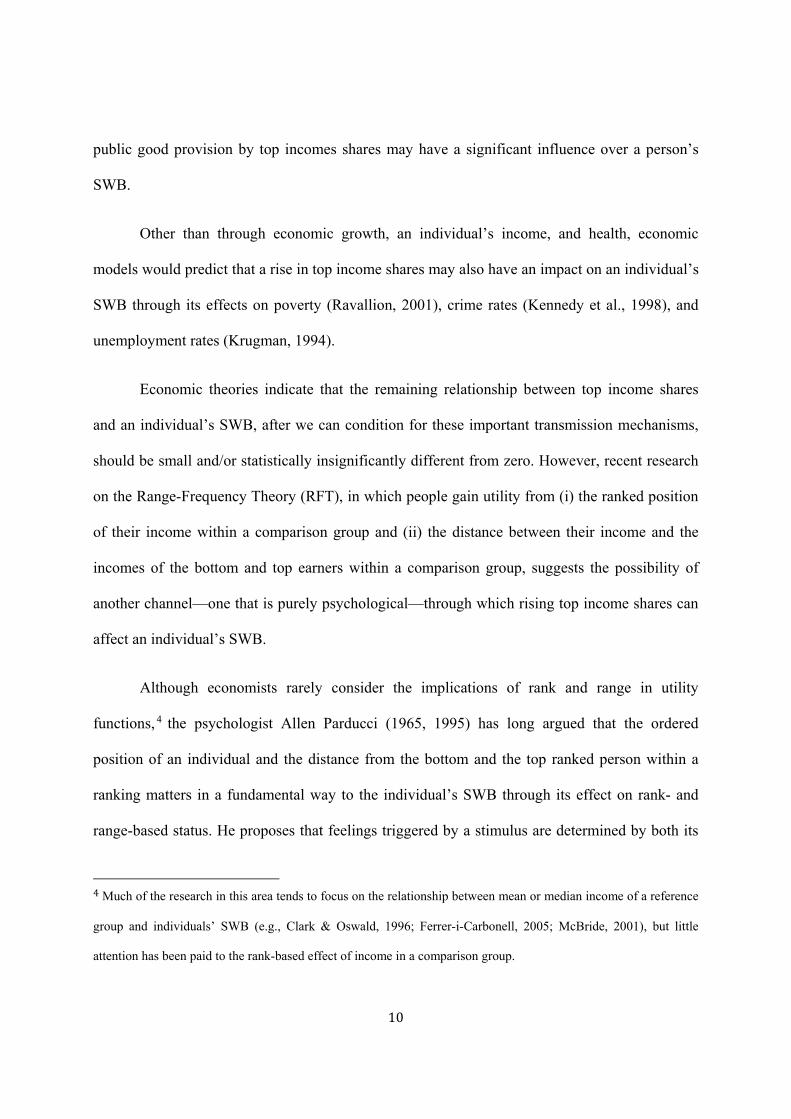
public good provision by top incomes shares may have a significant influence over a person’s
SWB.
Other than through economic growth, an individual’s income, and health, economic
models would predict that a rise in top income shares may also have an impact on an individual’s
SWB through its effects on poverty (Ravallion, 2001), crime rates (Kennedy et al., 1998), and
unemployment rates (Krugman, 1994).
Economic theories indicate that the remaining relationship between top income shares
and an individual’s SWB, after we can condition for these important transmission mechanisms,
should be small and/or statistically insignificantly different from zero. However, recent research
on the Range-Frequency Theory (RFT), in which people gain utility from (i) the ranked position
of their income within a comparison group and (ii) the distance between their income and the
incomes of the bottom and top earners within a comparison group, suggests the possibility of
another channel—one that is purely psychological—through which rising top income shares can
affect an individual’s SWB.
Although economists rarely consider the implications of rank and range in utility
functions, 4 the psychologist Allen Parducci (1965, 1995) has long argued that the ordered
position of an individual and the distance from the bottom and the top ranked person within a
ranking matters in a fundamental way to the individual’s SWB through its effect on rank- and
range-based status. He proposes that feelings triggered by a stimulus are determined by both its
4Much of the research in this area tends to focus on the relationship between mean or median income of a reference
group and individuals’ SWB (e.g., Clark & Oswald, 1996; Ferrer-i-Carbonell, 2005; McBride, 2001), but little
attention has been paid to the rank-based effect of income in a comparison group.
11
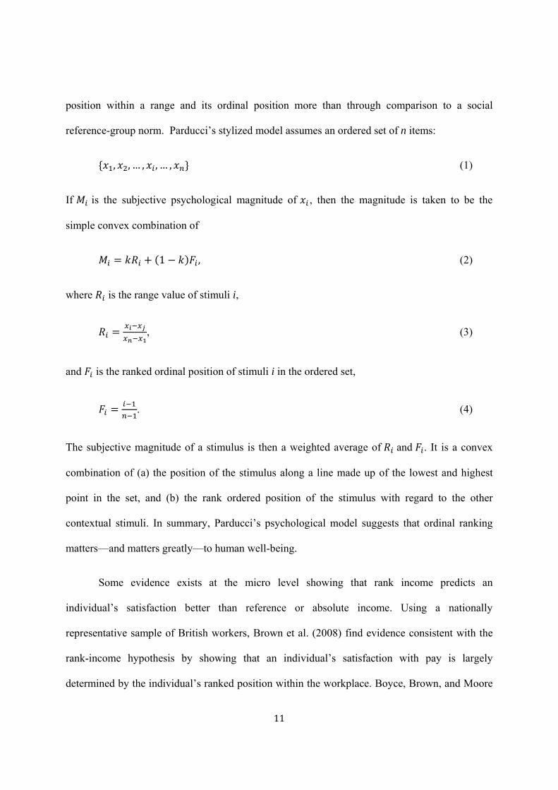
position within a range and its ordinal position more than through comparison to a social
reference-group norm. Parducci’s stylized model assumes an ordered set of n items:
, , … , , … , (1)
If is the subjective psychological magnitude of , then the magnitude is taken to be the
simple convex combination of
1 , (2)
where is the range value of stimuli i,
, (3)
and is the ranked ordinal position of stimuli i in the ordered set,
. (4)
The subjective magnitude of a stimulus is then a weighted average of and . It is a convex
combination of (a) the position of the stimulus along a line made up of the lowest and highest
point in the set, and (b) the rank ordered position of the stimulus with regard to the other
contextual stimuli. In summary, Parducci’s psychological model suggests that ordinal ranking
matters—and matters greatly—to human well-being.
Some evidence exists at the micro level showing that rank income predicts an
individual’s satisfaction better than reference or absolute income. Using a nationally
representative sample of British workers, Brown et al. (2008) find evidence consistent with the
rank-income hypothesis by showing that an individual’s satisfaction with pay is largely
determined by the individual’s ranked position within the workplace. Boyce, Brown, and Moore
12
(2010) show that the ranked position of an individual strongly predicts the individual’s life
satisfaction, but that absolute income and reference income have statistically insignificant
predictive power. Clark, Westergård-Nielsen, and Kristensen (2010) show that, conditional on
individuals’ own household income and neighborhood median income, individuals become more
satisfied with their income as their percentile neighborhood ranking improves. More recently,
Card et al. (2012) find that the effect of disclosing information on peers’ salaries on workers’ job
satisfaction is a function of the individual’s rank in the salary position rather than of the
individual’s relative pay level. They also find that the negative treatment effect is the largest
among workers in the lowest quintile of the pay distribution of their pay unit. However, the
economics literature is currently small, and evidence of rank-based comparison at the macro
level is virtually nonexistent.
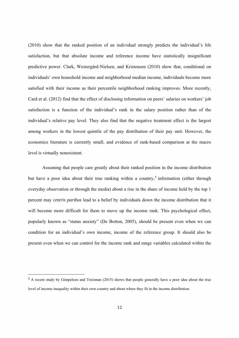
Assuming that people care greatly about their ranked position in the income distribution
but have a poor idea about their true ranking within a country,5 information (either through
everyday observation or through the media) about a rise in the share of income held by the top 1
percent may ceteris paribus lead to a belief by individuals down the income distribution that it
will become more difficult for them to move up the income rank. This psychological effect,
popularly known as “status anxiety” (De Botton, 2005), should be present even when we can
condition for an individual’s own income, income of the reference group. It should also be
present even when we can control for the income rank and range variables calculated within the
5A recent study by Gimpelson and Treisman (2015) shows that people generally have a poor idea about the true
level of income inequality within their own country and about where they fit in the income distribution.
13
survey sample, because it is the size of the top income shares of people who are less likely to be
included in the survey that actually matters to the individual’s psyche.6
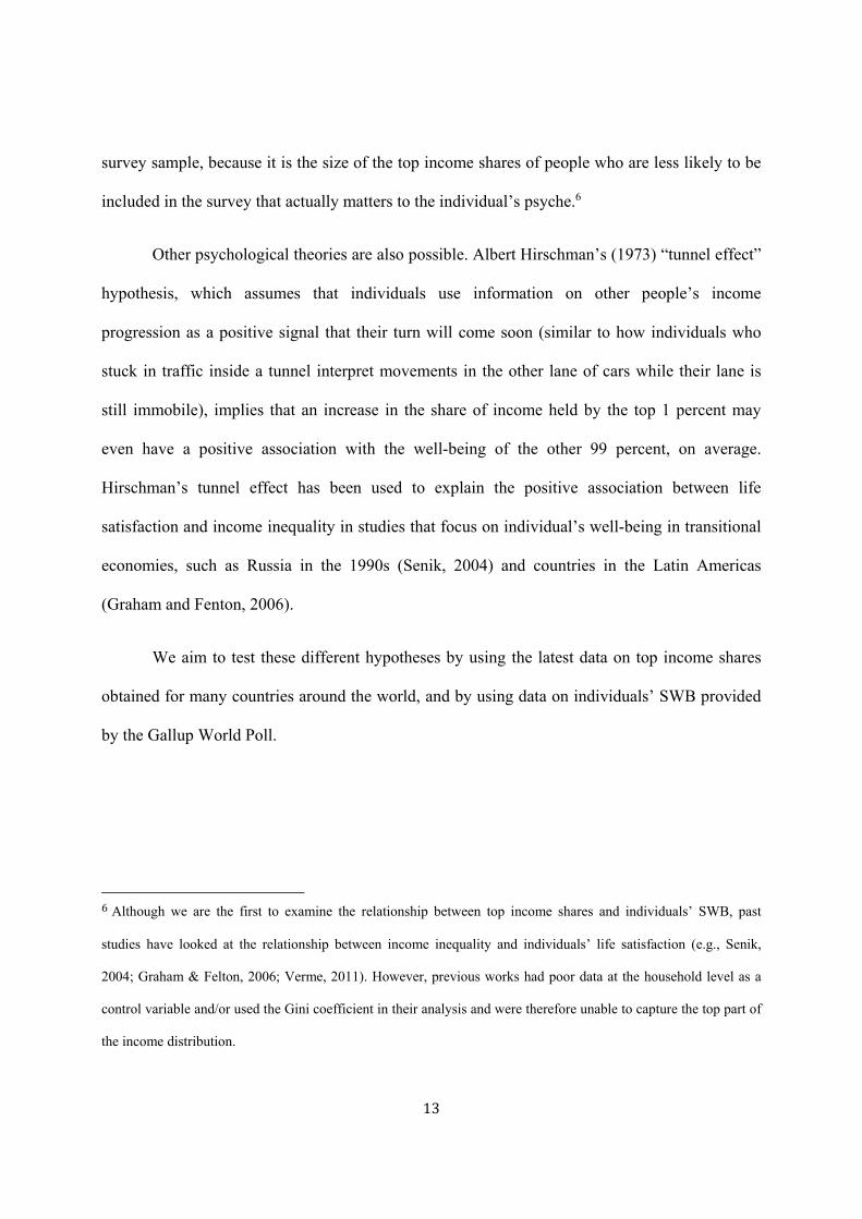
Other psychological theories are also possible. Albert Hirschman’s (1973) “tunnel effect”
hypothesis, which assumes that individuals use information on other people’s income
progression as a positive signal that their turn will come soon (similar to how individuals who
stuck in traffic inside a tunnel interpret movements in the other lane of cars while their lane is
still immobile), implies that an increase in the share of income held by the top 1 percent may
even have a positive association with the well-being of the other 99 percent, on average.
Hirschman’s tunnel effect has been used to explain the positive association between life
satisfaction and income inequality in studies that focus on individual’s well-being in transitional
economies, such as Russia in the 1990s (Senik, 2004) and countries in the Latin Americas
(Graham and Fenton, 2006).
We aim to test these different hypotheses by using the latest data on top income shares
obtained for many countries around the world, and by using data on individuals’ SWB provided
by the Gallup World Poll.
6Although we are the first to examine the relationship between top income shares and individuals’ SWB, past
studies have looked at the relationship between income inequality and individuals’ life satisfaction (e.g., Senik,
2004; Graham & Felton, 2006; Verme, 2011). However, previous works had poor data at the household level as a
control variable and/or used the Gini coefficient in their analysis and were therefore unable to capture the top part of
the income distribution.
14
III. Data
Our primary data come from the Gallup World Poll (GWP). Established in 2005 by the
Gallup Organization, the GWP continually surveys citizens in more than 150 countries around
the world and interviews approximately 1,000 residents per country. Respondents in the GWP
are randomly selected adults 15 years of age and older and are nationally representative. Gallup
asks each respondent the survey questions in the respondent’s language. The mode of the
interview is telephone survey in countries where telephone coverage represents at least 80% of
the population. Where telephone penetration is less than 80%, Gallup uses face-to-face
interviewing.
The GWP contains a wide range of questions about the respondent’s well-being. Life
evaluation, which is a measure of a person’s thoughts about his or her life, is elicited using the
Cantril life ladder question. The exact wording of the Cantril life ladder is “Please imagine a
ladder/mountain with steps numbered from zero at the bottom to ten at the top. Suppose we say
that the top of the ladder/mountain represents the best possible life for you and the bottom of the
ladder/mountain represents the worst possible life for you. If the top step is 10 and the bottom
step is 0, on which step of the ladder/mountain do you feel you personally stand at the present
time?” The corresponding response categories range from 0 (Worst possible life) to 10 (Best
possible life).
There are two measures of emotional well-being—positive and negative emotional
experience. Positive emotional experience (or positive experience index) is a measure of
respondents’ experienced well-being on the day before the survey. Questions provide a real-time
measure of respondents’ positive experiences and include the following: “Did you feel well-
15
rested yesterday?”, “Were you treated with respect all day yesterday?”, “Did you smile or laugh
a lot yesterday?”, “Did you learn or do something interesting yesterday?”, and “Did you
experience the following feelings during a lot of the day yesterday? How about enjoyment?” The
five items are recoded so that positive answers are scored as a “1” and all other answers
(including “don’t know” and “refused”) are scored as a “0.” An individual record has an index
calculated if it has at least four out of five valid scores (0 or 1). The final score is the mean of
valid items multiplied by 100.
Negative emotional experience is a real-time measure of respondents’ negative
experiences on the day before the survey. The index contains the following questions: “Did you
experience the following feelings during a lot of the day yesterday? How about physical pain?”,
“How about worry?”, “How about sadness?”, “How about stress?”, and “How about anger?”
The five items are recoded so that affirmative answers are scored as a “1” and all other answers
(including “don’t know” or “refused”) are a “0.” An individual record has an index calculated if
it has at least four out of five valid scores (0 or 1). The final score is the mean of valid items
multiplied by 100.
The distinction between life evaluation and emotional well-being was the focus of a
seminal study by Daniel Kahneman and Angus Deaton (2010), who find life evaluation to be
sensitive to an individual’s socio-economic status such as income and employment status,
whereas measures of emotional well-being are sensitive to circumstances that evoke emotional
responses, such as time spent commuting and caring for others.
16
Historical time-series data on the share of taxable national income (excluding capital
gains) held by the top 1 percent at the country level come from the WTID
(www.topincomes.parisschoolofeconomics.eu).
To control for movements in other country-level variables, historical time-series data on
macroeconomic variables (e.g., GDP per capita, annual GDP growth, unemployment rates,
inflation rates, public expenditure on health and education, and intentional homicide rates) are
obtained from the World Bank Database (www.data.worldbank.org). We also obtained time-
series data on the Corruption Index from Transparency International
(http://www.transparency.org) and the Human Development Index from the United Nations
Development Programme (http://hdr.undp.org/en/data).
We use seven waves of the GWP (2006–2012). Of the 31 countries available in the
WTID, 24 have the information on the top income share at the country level between 2006 and
2012 for the countries surveyed in the GWP. This produces 105 country-year data points at the
first instance. We then further restrict the GWP data to countries that have collected information
on individuals’ SWB, household income, and other personal characteristics. Our linked data thus
provide us with a series of repeated cross-sections between 2006 and 2012 on approximately
69,000 adults (15 years of age and older) from 22 countries—Australia, Canada, Colombia,
Denmark, Finland, France, Germany, Ireland, Italy, Japan, Malaysia, Netherlands, New Zealand,
Norway, Singapore, South Africa, South Korea, Spain, Sweden, Switzerland, Great Britain, and
the U.S.A.—which we use in our analysis. This leaves us with 66 country-year data points when
personal characteristics and other macroeconomic variables are taken into account. Tables 1A
and 2A in the Online Appendix describe the variables, as well as the means in the data set and
the survey years used in our analysis. Roughly 57% of the sample is female, and the average age
17
is approximately 47 years. Measures of SWB are standardized across the entire population to
have a mean of zero and a standard deviation of 1. The average income share held by the top 1
percent across the entire sample is 11.24% with a between-country standard deviation of 4.11.
However, note that the within-country variation is small (within-country standard deviation =
0.42) because our GWP time series is short.
IV. Empirical Strategy
For our cross-country analysis, we estimate the following regression equation:
Top1percent , (5)
where is a measure of SWB (i.e., life evaluation, positive experiences, and negative
experiences) of individual i in country j and year t. Top1percent is the share of taxable income
held by the top 1 percent in country j and year t. is a vector of individual characteristics that
includes the individual’s age, age squared, age cubed, log of real household income per capita
(2010 purchasing power parity-adjusted), log of average real household income per capita of
“someone like me” (i.e., same age bracket, gender, education level, country, and survey year),
Parducci’s income rank and range variables – see Eqs. (3) and (4) – calculated within the survey
sample by country and year, physical health index, number of children under the age of 15 years,
and dummy variables for self-employed, employed part-time but do not want full-time job,
unemployed, employed part-time but want full-time job, completed secondary/tertiary school,
completed high-school/college degree, married, separated, divorced, widowed, domestic partner,
and a dummy for whether the respondent is religious. is a vector of country-year variables,
including log of real GDP per capita, annual GDP growth, total unemployment rate, inflation rate
(based on Consumer Price Index), total government expenditures on health and primary
18
education, intentional homicide rate (per 100,000 people), Corruption Index, and Human
Development Index. is a set of continent dummies (North America, South America, Asia,
Australia/Oceania, and Africa, with Europe as the excluded reference group), which will be
replaced by country-specific dummies in later analysis. denotes a set of year dummies.
Finally, is the error term.
All regressions are estimated using ordinary least squares with standard errors adjusted
for clustering at the country year level.7 All regressions are also estimated with sampling
weights, although qualitatively similar results can still be obtained without adjusting for
sampling weights. In addition to the GWP results, we also estimate a similar econometric model
using the British Household Panel Study (BHPS), a long-running British longitudinal survey.
V. Results
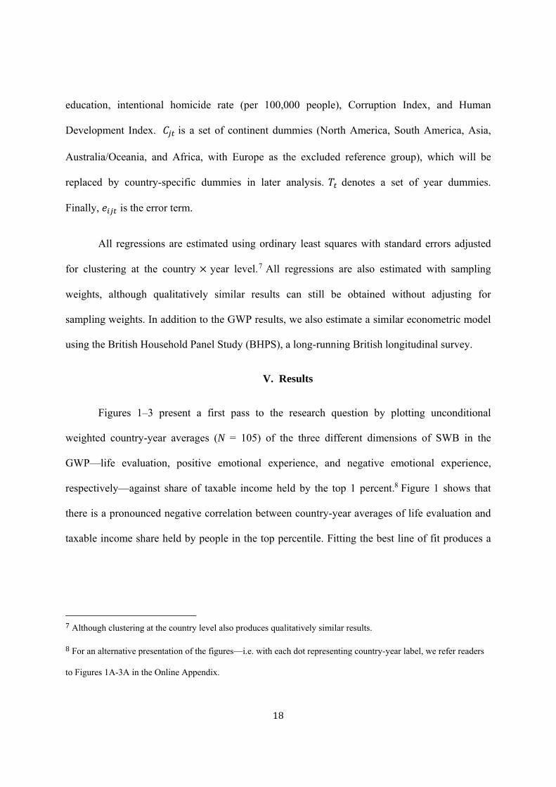
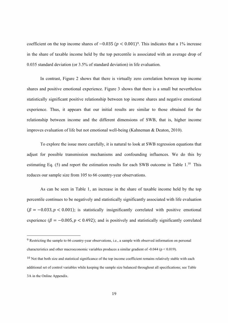
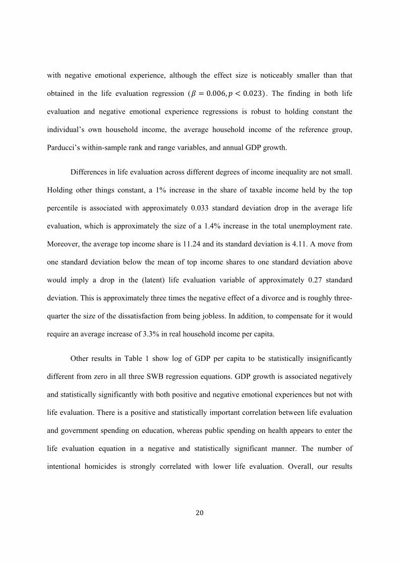
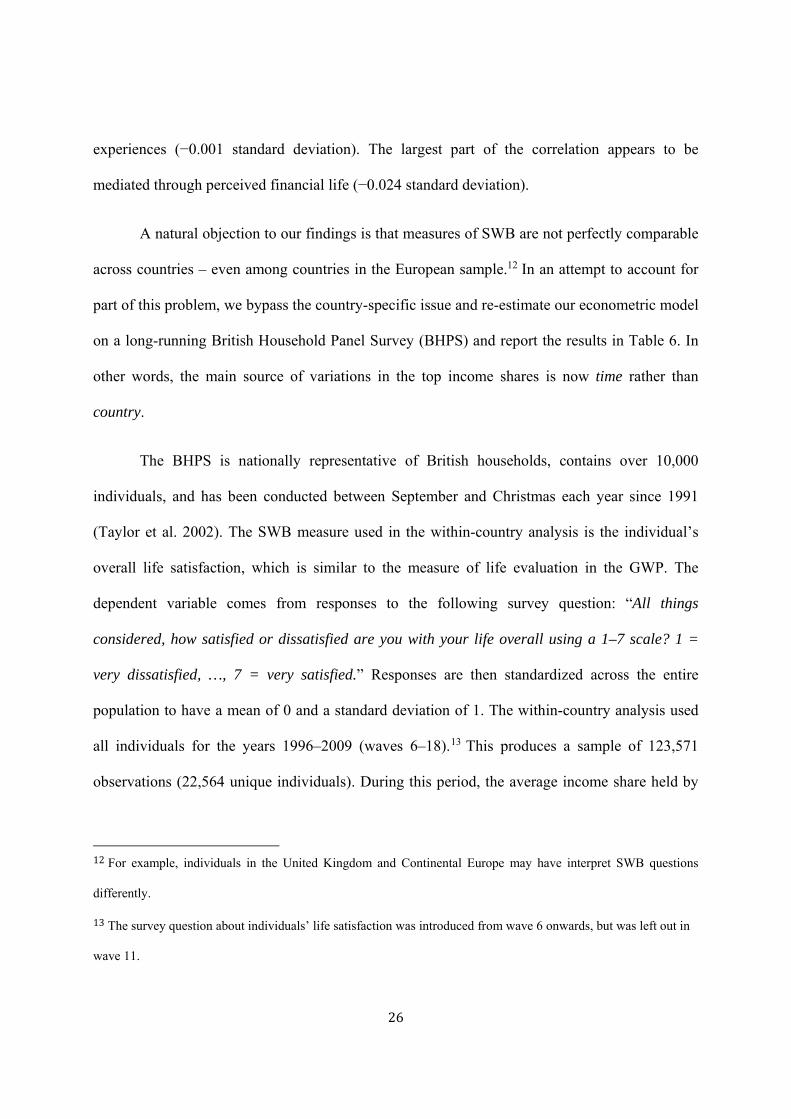
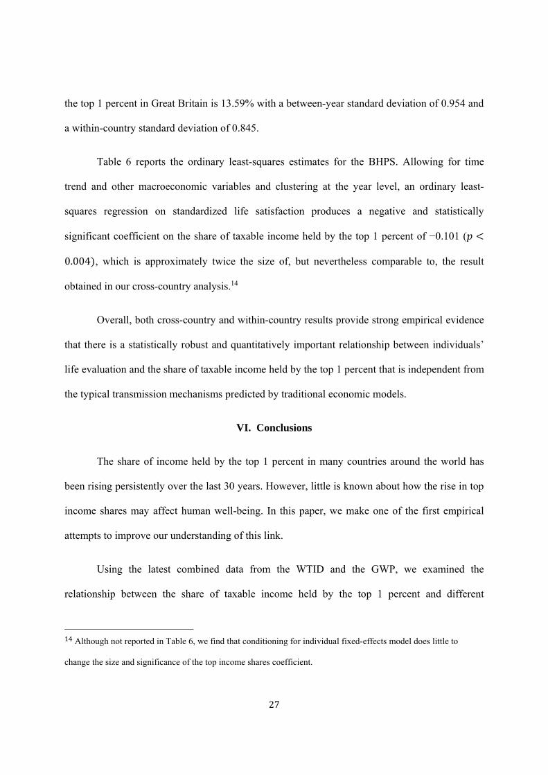
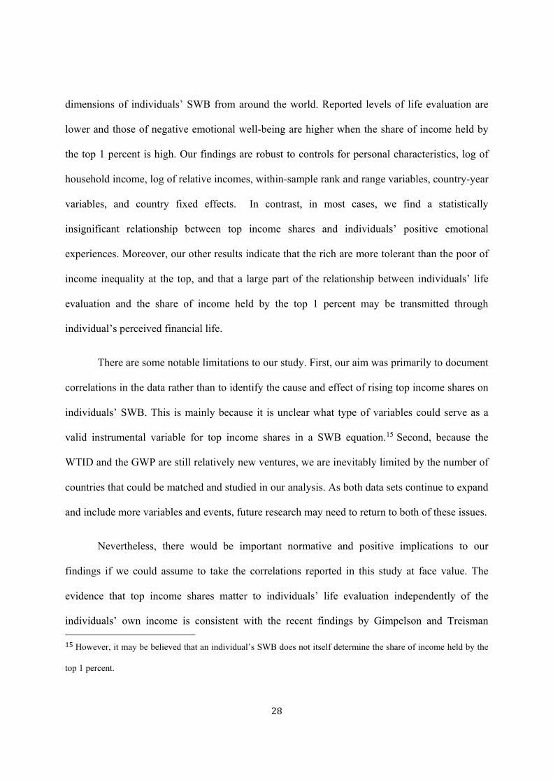
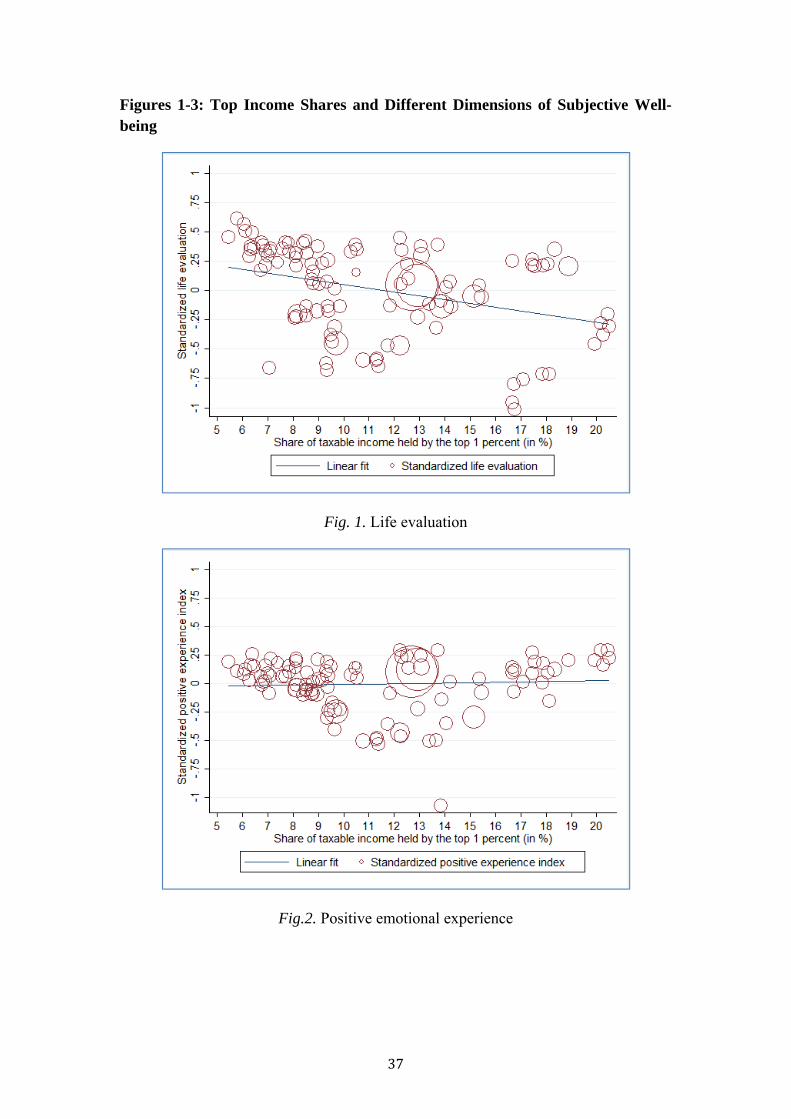
Figures 1–3 present a first pass to the research question by plotting unconditional
weighted country-year averages (N = 105) of the three different dimensions of SWB in the
GWP—life evaluation, positive emotional experience, and negative emotional experience,
respectively—against share of taxable income held by the top 1 percent.8 Figure 1 shows that
there is a pronounced negative correlation between country-year averages of life evaluation and
taxable income share held by people in the top percentile. Fitting the best line of fit produces a
7Although clustering at the country level also produces qualitatively similar results.
8For an alternative presentation of the figures—i.e. with each dot representing country-year label, we refer readers
to Figures 1A-3A in the Online Appendix.
19
coefficient on the top income shares of 0.035 0.001 9. This indicates that a 1% increase
in the share of taxable income held by the top percentile is associated with an average drop of
0.035 standard deviation (or 3.5% of standard deviation) in life evaluation.
In contrast, Figure 2 shows that there is virtually zero correlation between top income
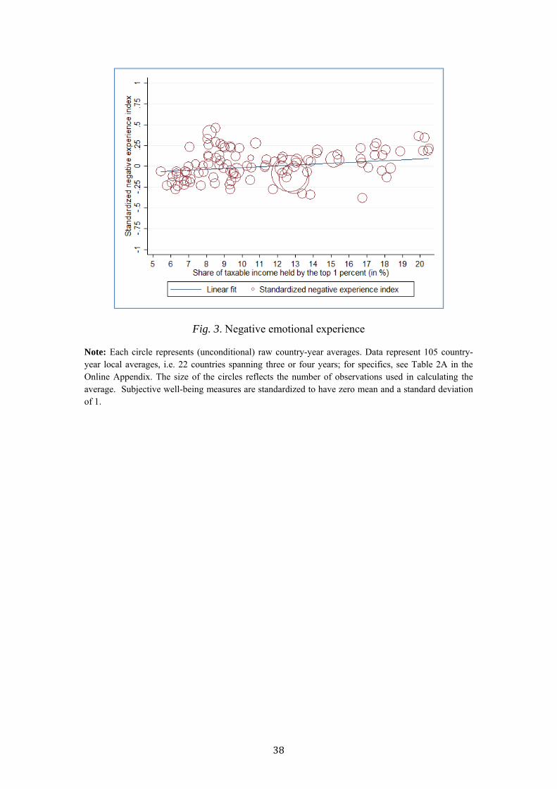
shares and positive emotional experience. Figure 3 shows that there is a small but nevertheless
statistically significant positive relationship between top income shares and negative emotional
experience. Thus, it appears that our initial results are similar to those obtained for the
relationship between income and the different dimensions of SWB, that is, higher income
improves evaluation of life but not emotional well-being (Kahneman & Deaton, 2010).
To explore the issue more carefully, it is natural to look at SWB regression equations that
adjust for possible transmission mechanisms and confounding influences. We do this by
estimating Eq. (5) and report the estimation results for each SWB outcome in Table 1.10 This
reduces our sample size from 105 to 66 country-year observations.
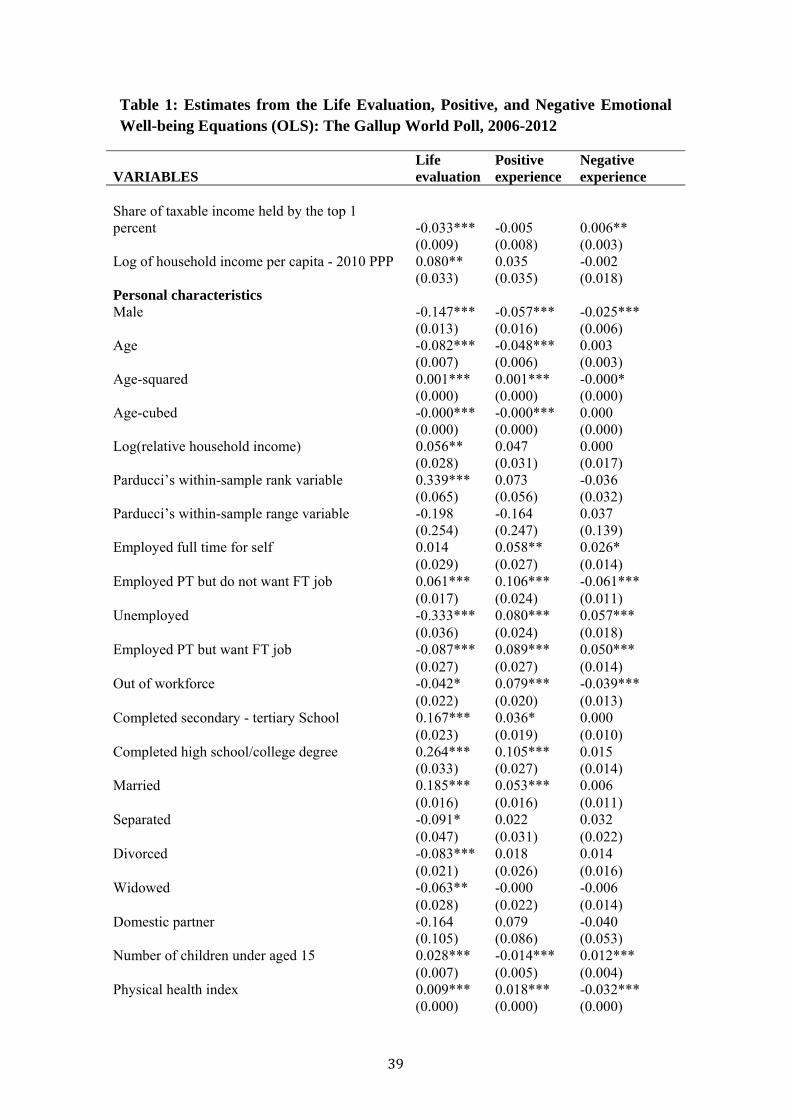
As can be seen in Table 1, an increase in the share of taxable income held by the top
percentile continues to be negatively and statistically significantly associated with life evaluation
0.033, 0.001 ; is statistically insignificantly correlated with positive emotional
experience ( 0.005, 0.492 ; and is positively and statistically significantly correlated
9Restricting the sample to 66 country-year observations, i.e., a sample with observed information on personal
characteristics and other macroeconomic variables produces a similar gradient of -0.044 (p < 0.019).
10Not that both size and statistical significance of the top income coefficient remains relatively stable with each
additional set of control variables while keeping the sample size balanced throughout all specifications; see Table
3A in the Online Appendix.
20
with negative emotional experience, although the effect size is noticeably smaller than that
obtained in the life evaluation regression ( 0.006, 0.023 . The finding in both life
evaluation and negative emotional experience regressions is robust to holding constant the
individual’s own household income, the average household income of the reference group,
Parducci’s within-sample rank and range variables, and annual GDP growth.
Differences in life evaluation across different degrees of income inequality are not small.
Holding other things constant, a 1% increase in the share of taxable income held by the top
percentile is associated with approximately 0.033 standard deviation drop in the average life
evaluation, which is approximately the size of a 1.4% increase in the total unemployment rate.
Moreover, the average top income share is 11.24 and its standard deviation is 4.11. A move from
one standard deviation below the mean of top income shares to one standard deviation above
would imply a drop in the (latent) life evaluation variable of approximately 0.27 standard
deviation. This is approximately three times the negative effect of a divorce and is roughly three-
quarter the size of the dissatisfaction from being jobless. In addition, to compensate for it would
require an average increase of 3.3% in real household income per capita.
Other results in Table 1 show log of GDP per capita to be statistically insignificantly
different from zero in all three SWB regression equations. GDP growth is associated negatively
and statistically significantly with both positive and negative emotional experiences but not with
life evaluation. There is a positive and statistically important correlation between life evaluation
and government spending on education, whereas public spending on health appears to enter the
life evaluation equation in a negative and statistically significant manner. The number of
intentional homicides is strongly correlated with lower life evaluation. Overall, our results
21
indicate that top income shares are one of the most important country-level predictors of
international differences in life evaluation.
A natural next step is to examine whether the estimated relationship between top income
shares and SWB will continue to be statistically robust after controlling for country-specific
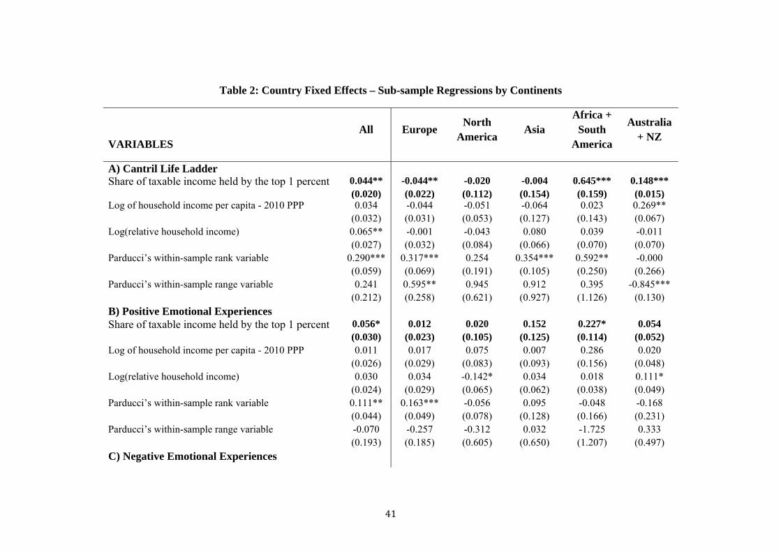
dummies. As a check, Table 2 presents country fixed effects estimates for all individuals and by
continents—Europe, North America, Asia, Australia/NZ, and Africa/South America.
Unfortunately, because of the small number of countries in our sample in most of our continents
(i.e. North America, Africa, Australia/Oceania, South America), we were unable to obtain
estimates of the top income share in these continents when macroeconomic conditions are
controlled for in the regression.
Table 2 contains a number of findings that might have been hard to predict. Conditioning
on country fixed effects, Column 1 of Panel A shows that individuals are apparently reporting
higher levels of life evaluation as the within-country share of income held by the top 1 percent
increases: the coefficient on top income shares is 0.044 0.032 . What this result implies is
that a short-run increase in the top income shares may on average be taken as a signal to
individuals across the entire sample that it might soon be their turn, which would be more
consistent with Hirschman’s “tunnel effect” hypothesis (Hirschman, 1973). Nevertheless, a look
across columns of sub-sample regressions seems to suggest that this finding is driven primarily
by the relationship between top income shares and life evaluation in less-developed economies
such as Colombia and South Africa, but also in Australia and New Zealand. The coefficient on
top income share in the life evaluation equation continues to be negative in three out of five sub-
samples—Europe, North America, and Asia. However, given the small number of country-year
data in four out of five (North America, Asia, Africa/South America, Australia/NZ) sub-sample
22
analysis, the coefficients on top income for these sub-samples should be treated with care. Note
also that in Europe where we do have enough countries to also control for macro effects we
continue to find that top income share is negative and statistically significant and increased by
approximately 30% (from -0.033 to -0.044).
Table 2’s other results also suggest a positive and marginally statistically significant
association between within-country changes in the top income shares and positive emotional
experiences when the entire sample is used in the estimation. Again, the full sample results seem
to be driven primarily by countries in Africa and South America.
Given that our preferred specification is one that controls for country-specific dummies,
the next three tables will focus only on the European sample where populations from different
countries are similar to each other and we do have enough countries to run country fixed effects
regressions.
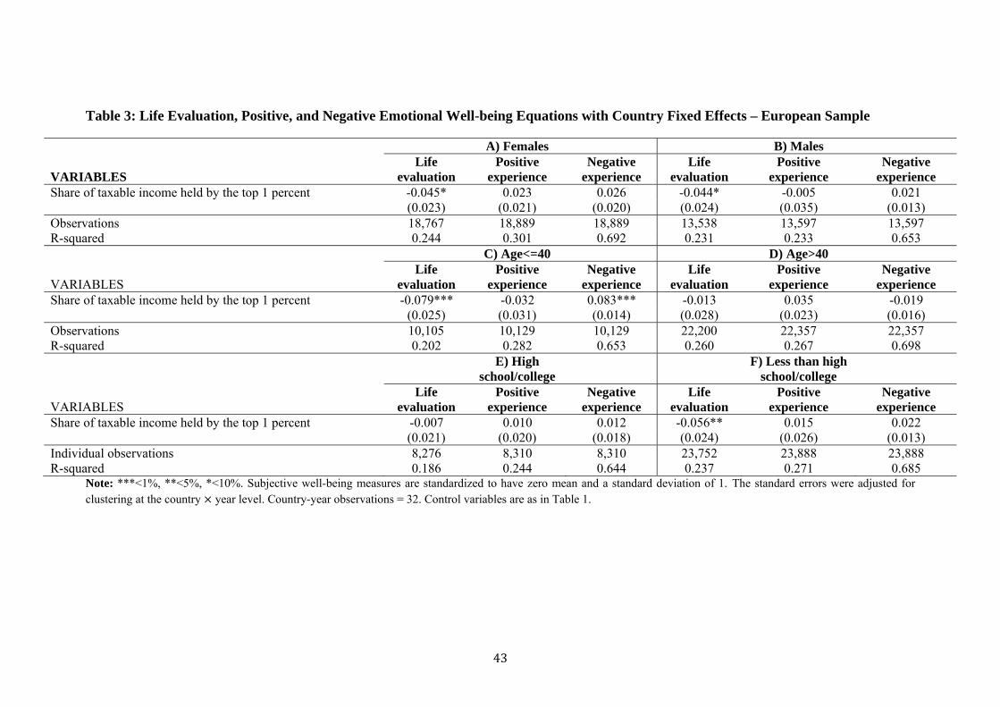
Our next empirical analysis is to test whether the estimated relationship between top
income shares and SWB varies across subsamples of the population. In Table 3 we do this by
separating the data by gender, age group, and education level. Looking across columns, it can be
seen that the share of taxable income held by the top 1 percent continues to enter the life
evaluation regression equation in a negative and statistically significant manner for all subgroups
of the population. First, we cannot reject the null hypothesis that the paired coefficients are the
same between male and female sub-samples. There is, however, some evidence of heterogeneity
by age group and educational group in the life evaluation and negative emotional experience
regressions. For the old versus the young sub-sample regressions, we find an increase in the top
income shares appears to be statistically significantly correlated with lower life evaluation (
23
0.079, 0.004) and higher negative emotional experiences for the younger age group (
0.083, 0.001), whereas the same coefficients are statistically insignificantly different from
zero for the older age group. For the low versus high education sub-sample regressions, we find
an increase in the top income shares appears to be statistically significantly correlated with lower
life evaluation for the high school/college graduates ( 0.056, 0.024), whereas the
same coefficient is statistically insignificantly different from zero for the less than high
school/college graduates ( 0.007, 0.747).
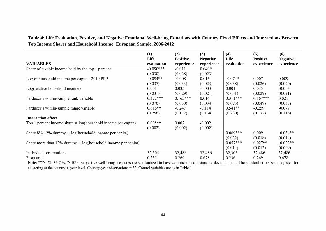
Table 4 tests whether the rich are more satisfied than the poor when top income share is
high. The first three columns of Table 4 do this by examining the interaction between share of
taxable income held by the top 1 percent and log of real household income per capita. It can be
seen that the interaction term is positive and statistically significant in the life evaluation
regression ( 0.005, 0.028 , whereas it is statistically insignificantly different from zero
in both positive and negative emotional experiences regressions. For life evaluation, the
coefficient on share of taxable income held by the top 1 percent is negative and statistically
significant at −0.094 ( 0.016 . This implies that when individuals’ own household income is
held constant, an increase in top income share would hurt the rich less than it would hurt the
poor. The estimates also imply that individuals who earn 18.8% higher income than the mean
value will feel indifferent by a 1% increase in the top income share ( 0.094 0.005 18.8
0 . Interestingly the main effect of income is negative and statistically significant, although this
could be explained partly by the fact that rank and range variables are being held constant in the
regression. In other words, an increase in household income that does not lead to an
improvement in income rank is associated negatively with life evaluation. By contrast, both rank
and range variables are positively and statistically significantly associated with life evaluation,
24
which is consistent with previous evidence in the psychology literature (e.g., Brown et al., 2008;
Boyce et al., 2010).
We then divide our countries into three groups based on the share of income held by their
top income group: below 8%, between 8% and 12%, and greater than 12%. We then put the first
group in the constant and create dummy variables for the others to replace our continuous top
income share variable and report the estimates in the last three columns of Table 4. Qualitatively
similar results can still be obtained using this specification. It can also be seen that, although a
rise in top income share is associated positively and statistically significantly with negative
emotional experiences, some evidence indicates that the estimated effect may be smaller for the
rich than for the poor.
So far our results indicate a strong negative relationship between individuals’ life
evaluation and the share of income held by the top 1 percent that is robust to household income,
socio-economic status, and other macroeconomic controls. The estimated gradient has also
changed little from a bivariate model to a regression with a full set of control variables (a change
from −0.034 (N = 105 country-year) to −0.033 in the full sample (N = 66 country-year), and in
−0.044 the European sample (N = 32 country-year) with country fixed effects). However, there
may be other transmission mechanisms—other than the pure psychological effect of rank-based
status—that have not been properly captured under the current specification, including, for
example, the relationship between top income shares and social cohesion (Kawachi & Kennedy,
1997) or even with subjective poverty that is independent from income.
In an attempt to capture other possible transmission mechanisms, in Column 1 of Table 5
we introduce a range of individuals’ attitudes as potential mediators of top income shares in life
25
evaluation for the European sample. This includes community attachment, community basics,
civic engagement, diversity, law and order, financial life, food and shelter, national institutions,
corruption, optimism, and daily experiences.11 For ease of interpretation, all of the attitudinal
variables are standardized to have a mean of 0 and a standard deviation of 1.
After controlling for these possible mediators of top income shares, the coefficient on
share of taxable income held by the top 1 percent continues to be negative albeit statistically
insignificantly different from zero ( 0.030, 0.159 . Holding other variables constant,
life evaluation also correlates significantly with higher levels of community attachment,
community basics, civic engagement, diversity, financial life, food and shelter, optimism, and
daily experiences.
Column 2 of Table 5 reports the estimates on top income shares obtained from regressing
each of the attitude regression equations separately. Controlling for the same set of individuals’
socio-economic status, macroeconomic variables, and country-specific dummies as in the first
column, it can be seen that the share of taxable income held by the top 1 percent is statistically
significantly correlated with higher levels of perceived community basics and diversity; and is
negatively and statistically significantly associated with attitudes toward civic engagement, law
and order, financial life, national institution, and corruption. Finally, we present in Column 3 of
Table 5 the estimated indirect effects of top income shares on life evaluation through these
subjective channels. We find that only a small part of the correlation between top income shares
and life evaluation can be explained through reduced civic engagement (−0.004 standard
deviation), increased community basics (0.001 standard deviation), and negative daily
11Please refer to Table 1A in the Online Appendix for a full description of these attitude variables.
26
experiences (−0.001 standard deviation). The largest part of the correlation appears to be
mediated through perceived financial life (−0.024 standard deviation).
A natural objection to our findings is that measures of SWB are not perfectly comparable
across countries – even among countries in the European sample.12 In an attempt to account for
part of this problem, we bypass the country-specific issue and re-estimate our econometric model
on a long-running British Household Panel Survey (BHPS) and report the results in Table 6. In
other words, the main source of variations in the top income shares is now time rather than
country.
The BHPS is nationally representative of British households, contains over 10,000
individuals, and has been conducted between September and Christmas each year since 1991
(Taylor et al. 2002). The SWB measure used in the within-country analysis is the individual’s
overall life satisfaction, which is similar to the measure of life evaluation in the GWP. The
dependent variable comes from responses to the following survey question: “All things
considered, how satisfied or dissatisfied are you with your life overall using a 1–7 scale? 1 =
very dissatisfied, …, 7 = very satisfied.” Responses are then standardized across the entire
population to have a mean of 0 and a standard deviation of 1. The within-country analysis used
all individuals for the years 1996–2009 (waves 6–18).13 This produces a sample of 123,571
observations (22,564 unique individuals). During this period, the average income share held by
12For example, individuals in the United Kingdom and Continental Europe may have interpret SWB questions
differently.
13 The survey question about individuals’ life satisfaction was introduced from wave 6 onwards, but was left out in
wave 11.
27
the top 1 percent in Great Britain is 13.59% with a between-year standard deviation of 0.954 and
a within-country standard deviation of 0.845.
Table 6 reports the ordinary least-squares estimates for the BHPS. Allowing for time
trend and other macroeconomic variables and clustering at the year level, an ordinary least-
squares regression on standardized life satisfaction produces a negative and statistically
significant coefficient on the share of taxable income held by the top 1 percent of −0.101 (
0.004 , which is approximately twice the size of, but nevertheless comparable to, the result
obtained in our cross-country analysis.14
Overall, both cross-country and within-country results provide strong empirical evidence
that there is a statistically robust and quantitatively important relationship between individuals’
life evaluation and the share of taxable income held by the top 1 percent that is independent from
the typical transmission mechanisms predicted by traditional economic models.
VI. Conclusions
The share of income held by the top 1 percent in many countries around the world has
been rising persistently over the last 30 years. However, little is known about how the rise in top
income shares may affect human well-being. In this paper, we make one of the first empirical
attempts to improve our understanding of this link.
Using the latest combined data from the WTID and the GWP, we examined the
relationship between the share of taxable income held by the top 1 percent and different
14Although not reported in Table 6, we find that conditioning for individual fixed-effects model does little to
change the size and significance of the top income shares coefficient.
28
dimensions of individuals’ SWB from around the world. Reported levels of life evaluation are
lower and those of negative emotional well-being are higher when the share of income held by
the top 1 percent is high. Our findings are robust to controls for personal characteristics, log of
household income, log of relative incomes, within-sample rank and range variables, country-year
variables, and country fixed effects. In contrast, in most cases, we find a statistically
insignificant relationship between top income shares and individuals’ positive emotional
experiences. Moreover, our other results indicate that the rich are more tolerant than the poor of
income inequality at the top, and that a large part of the relationship between individuals’ life
evaluation and the share of income held by the top 1 percent may be transmitted through
individual’s perceived financial life.
There are some notable limitations to our study. First, our aim was primarily to document
correlations in the data rather than to identify the cause and effect of rising top income shares on
individuals’ SWB. This is mainly because it is unclear what type of variables could serve as a
valid instrumental variable for top income shares in a SWB equation.15 Second, because the
WTID and the GWP are still relatively new ventures, we are inevitably limited by the number of
countries that could be matched and studied in our analysis. As both data sets continue to expand
and include more variables and events, future research may need to return to both of these issues.
Nevertheless, there would be important normative and positive implications to our
findings if we could assume to take the correlations reported in this study at face value. The
evidence that top income shares matter to individuals’ life evaluation independently of the
individuals’ own income is consistent with the recent findings by Gimpelson and Treisman 15However, it may be believed that an individual’s SWB does not itself determine the share of income held by the
top 1 percent.
29
(2015) that it is the perceived inequality—rather than actual inequality—that determines
individuals’ demand for redistribution and reported conflict between the rich and the poor. Thus,
both our results lead us to argue that most theories on the political effects of inequality should be
re-evaluated to take into account the psychological model of rank-based status and the effects of
perceived inequality. Moreover, policy makers may need to start giving more weight to the
psychological values attached to the “top 1 percent” who are not normally representative in a
survey when designing redistributive policies.
In addition, our paper’s other main finding that top income shares matter more to life
evaluation than to emotional well-being contributes to the previous literature showing that the
main predictors of both positive and negative emotions are not a person’s socio-economic status
but everyday circumstances (e.g., Kahneman & Deaton, 2010). In other words, our results
indicate that as the share of income held by the top percentile grows, people’s use of time may
not have shifted sufficiently toward activities that significantly reduce positive emotional
experiences, therefore holding constant their budget constraints. The paper’s findings thus add to
the ongoing debate with respect to the question of whether life evaluation or emotional well-
being is better suited for use in the assessment of human welfare and to guide policy.
More generally, although recent studies in economics have provided evidence that the
rising top income shares have important consequences for human well-being, our study is the
first attempt to provide clear and direct evidence on this issue.
30
References
Adelmann, Irma, and Sherman Robinson, “Income Distribution and Development,” in Hollis
Chenery, and T.N. Srinivisan, eds., Handbook of Development Economics (New York:
North-Holland, 1989), 949–1003.
Aghion, Philippe, Eve Caroli, and Cecilia Garcia-Peñalosa, 1999. “Inequality and Economic
Growth: The Perspective of the New Growth Theories,” Journal of Economic Literature
37 (1999), 1615–1660.
Alesina, Alberto, Rafael Di Tella, and Robert MacCulloch. "Inequality and happiness: are
Europeans and Americans different?." Journal of Public Economics 88.9 (2004): 2009-
2042.
Alesina, Alberto, and Roberto Perotti, “Income Distribution, Political Instability, and
Investment,” European Economic Review 40 (1996), 1203–1228.
Alesina, Alberto, and Dani Rodrik, “Income Distribution and Economic Growth: A Simple
Theory and Some Empirical Evidence,” in Alex Cukierman, Zvi Hercovitz, and Leonardo
Leiderman, eds., The Political Economy of Business Cycles and Growth (Cambridge:
MIT Press, 1993).
Alesina, Alberto, and Dani Rodrik, “Distributive Politics and Economic Growth,” Quarterly
Journal of Economics 109 (1994), 465–490.
Andrews, Dan, Christopher Jencks, and Andrew Leigh, “Do Rising Top Incomes Lift All
Boats?” The BE Journal of Economic Analysis & Policy 11 (2011), Article 6.
31
Araujo, M. Caridad, Francisco H.G. Ferreira, Peter Lanjouw, and Berk Özler, “Local Inequality
and Project Choice: Theory and Evidence from Ecuador,” Journal of Public Economics
92 (2008), 1022–1046.
Atkinson, Anthony B., and Andrea Brandolini. "Promise and pitfalls in the use of" secondary"
data-sets: Income inequality in OECD countries as a case study." Journal of economic
literature (2001): 771-799.
Atkinson, Anthony B., Thomas Piketty, and Emmanuel Saez, “Top Incomes in the Long Run of
History,” Journal of Economic Literature 49 (2011): 3–71.
Bénabou, Roland, “Inequality, Technology and the Social Contract,” in P. Aghion, and S.N.
Durlauf, eds., Handbook of Economic Growth (Amsterdam: Elsevier, 2005), Volume 1,
Part 2, 1595-1638
Blanchflower, David, and Andrew Oswald. "Does Inequality Reduce Happiness? Evidence from
the States of the USA from the 1970s to the 1990s." Mimeographed, Warwick University
(2003).
Boyce, Christopher J., Gordon D. Brown, and Simon C. Moore, “Money and Happiness Rank of
Income, not Income, Affects Life Satisfaction,” Psychological Science 21 (2010), 471–
475.
Brown, Gordon D., Jonathan Gardner, Andrew J. Oswald, and Jing Qian, “Does Wage Rank
Affect Employees’ Well‐being?” Industrial Relations: A Journal of Economy and
Society 47 (2008), 355–389.
32
Burkhauser, Richard V., Shuaizhang Feng, Stephen P. Jenkins, and Jeff Larrimore, “Recent
Trends in Top Income Shares in The United States: Reconciling Estimates from March
CPS and IRS Tax Return Data,” Review of Economics and Statistics 94 (2012), 371–388.
Card, David, Alexandre Mas, Enrico Moretti, and Emmanuel Saez, “Inequality at Work: The
Effect of Peer Salaries on Job Satisfaction,” American Economic Review 102 (2012),
2981–3003.
Clark, George R.G., “More Evidence on Income Distribution and Growth,” Journal of
Development Economics 47 (1995), 403–427.
Clark, Andrew E., Paul Frijters and Michael A. Shields, “Relative Income, Happiness, and
Utility: An Explanation for the Easterlin Paradox and Other Puzzles,” Journal of
Economic Literature 46 (2008), 95–144.
Clark, Andrew E., and Andrew J. Oswald, “Satisfaction and Comparison Income,” Journal of
Public Economics 61 (1996), 359–381.
Clark, Andrew E., Niels Westergård‐Nielsen, and Nicolai Kristensen, “Economic Satisfaction
and Income Rank in Small Neighbourhoods,” Journal of the European Economic
Association 7 (2009), 519–527.
De Botton, Alain. Status Anxiety (London: Penguin, 2005).
De Neve, Jan-Emmanuel, George Ward, Femke De Keulenaer, Bert Van Landeghem, Georgios
Kavetsos, and Michael I. Norton, “The Asymmetric Experience of Positive and Negative
Economic Growth: Global Evidence Using Subjective Well-Being Data,” London School
33
of Economics and Political Science, Centre for Economic Performance Discussion Paper
No.1304 (2014).
Deaton, Angus. The Great Escape: Health, Wealth, and the Origins of Inequality (Princeton, NJ:
Princeton University Press, 2013).
Deininger, Klaus, and Lyn Squire, “New Ways of Looking at Old Issues: Inequality and
Growth,” Journal of Development Economics 57 (1998), 259–287.
Easterlin, Richard A., “Does Economic Growth Improve the Human Lot? Some Empirical
Evidence,” Nations and Households in Economic Growth 89 (1974), 89–125.
Easterlin, Richard A., “Will Raising the Incomes of All Increase the Happiness of All?” Journal
of Economic Behavior & Organization 27 (1995), 35–47.
Enns, Peter K., Nathan J. Kelly, Jana Morgan, Thomas Volscho, and Christopher Witko,.
“Conditional Status Quo Bias and Top Income Shares: How US Political Institutions
Have Benefited the Rich,” Journal of Politics 76 (2014), 289–303.
Ferrer-i-Carbonell, Ada, “Income and Well-being: An Empirical Analysis of the Comparison
Income Effect,” Journal of Public Economics 89 (2005), 997–1019.
Ferrer-i-Carbonell, Ada, and Xavier Ramos. Inequality aversion and risk attitudes. IZA
Discussion Paper No. 4703 (2009).
Ferrer-i-Carbonell, Ada, and Xavier Ramos. Inequality and happiness. Journal of Economic
Surveys 28 (2014), 1016-1027.
Forbes, Kristin, “A Reassessment of the Relationship Between Inequality and Growth,”
American Economic Review 90 (2000), 869–887.
34
Galor, Oded, and Joseph Zeira, “Income Distribution and Macroeconomics,” Review of
Economic Studies 60 (1993), 35–52.
Gimpelson, Vladimir, and Daniel Treisman, “Misperceiving Inequality,” NBER Working Paper
21174 (2015).
Graham, Carol, and Andrew Felton, “Inequality and Happiness: Insights from Latin America,”
Journal of Economic Inequality 4 (2006): 107–122.
Halter, Daniel, Manuel Oechslin, and Josef Zweimüller, “Inequality and Growth: The Neglected
Time Dimension,” Journal of Economic Growth 19 (2014), 81–104.
Hirschman, Albert O. “The Changing Tolerance for Income Inequality in the Course of
Economic Development”, with a mathematical appendix by Michael Rothschild.
Quarterly Journal of Economics 87 (1973): 544–566
Jiang, Shiqing, Ming Lu, and Hiroshi Sato. "Identity, inequality, and happiness: Evidence from
urban China." World Development 40.6 (2012): 1190-1200.
Kahneman, Daniel, and Angus Deaton, “High Income Improves Evaluation of Life but not
Emotional Well-Being,” Proceedings of the National Academy of Sciences of the United
States of America 107 (2010), 16489–16493.
Kaldor, Nicholas, “A Model for Economic Growth,” Economic Journal 67 (1957), 591–624.
Kawachi, Ichiro, and Bruce P. Kennedy, “Socioeconomic Determinants of Health: Health and
Social Cohesion: Why Care About Income Inequality?” British Medical Journal 314
(1997), 1037.

35
Kennedy, Bruce P., Ichiro Kawachi, Deborah Prothrow-Stith, Kimberly Lochner, and Vanita
Gupta, “Social Capital, Income Inequality, and Firearm Violent Crime,” Social Science &
Medicine 47 (1998), 7–17.
Krugman, Paul, “Past and Prospective Causes of High Unemployment,” Economic Review-
Federal Reserve Bank of Kansas City 79 (1994), 23–43.
Leigh Andrew, “How Closely Do Top Income Shares Track Other Measures of Inequality?”
Economic Journal 117 (2007), F619–F633.
Li, Hongyi and Heng-fu Zou, “Income Inequality Is Not Harmful for Growth: Theory and
Evidence,” Review of Development Economics 2 (1998), 318–334.
Lillard Dean R., Richard V. Burkhauser, Marcus H. Hahn, and Roger Wilkins, “Does Early-Life
Income Inequality Predict Self-Reported Health in Later Life?” Social Science &
Medicine 128 (2015), 347–355.
McBride, Michael, “Relative-Income Effects on Subjective Well-Being in the Cross-Section,”
Journal of Economic Behavior and Organization 45 (2001), 251–278.
Oishi, Shigehiro and Selin Kesebir, “Income Inequality Explains Why Economic Growth Does
Not Always Translate to an Increase in Happiness,” Psychological Science, forthcoming.
Parducci, Allen, “Category Judgment: A Range-Frequency Model,” Psychological Review 72
(1965), 407–418.
Parducci, Allen, Happiness, Pleasure, and Judgment: The Contextual Theory and Its
Applications (Mahwah, NJ: Lawrence Erlbaum Associates Publishers, 1995).

36
Persson, Torsten, and Guido Tabellini, “Is Inequality Harmful for Growth?” American Economic
Review 84 (1994), 600–621.
Piketty, Thomas, and Emmanuel Saez, “Inequality in the Long Run.” Science 344 (2014), 838–
843.
Ravallion, Martin, “Growth, Inequality and Poverty: Looking Beyond Averages,” World
Development 29 (2001), 1803–1815.
Saint Paul, Giles, and Thierry Verdier, “Inequality, Redistribution and Growth: A Challenge to
the Conventional Political Economy Approach,” European Economic Review 40 (1996),
719–728.
Senik, Claudia, “When Information Dominates Comparison: Learning from Russian Subjective
Panel Data,” Journal of Public Economics 88 (2004), 2099–2123.
Schwarze, Johannes, and Marco Härpfer. "Are people inequality averse, and do they prefer
redistribution by the state?: evidence from german longitudinal data on life satisfaction."
The Journal of Socio-Economics 36.2 (2007): 233-249.
Taylor, Marcia F., John Brice, Nick Buck, and Elaine Prentice-Lane, British Household Panel
Survey User Manual (Colchester: University of Essex, 2002).
Verme, Paolo, “Life Satisfaction and Income Inequality,” Review of Income and Wealth 57
(2011), 111–127.
Wilkinson, Richard G., Unhealthy Societies: The Afflictions of Inequality (London: Routledge,
1996).
37
Figures 1-3: Top Income Shares and Different Dimensions of Subjective Well-being
Fig. 1. Life evaluation
Fig.2. Positive emotional experience
38
Fig. 3. Negative emotional experience
Note: Each circle represents (unconditional) raw country-year averages. Data represent 105 country-year local averages, i.e. 22 countries spanning three or four years; for specifics, see Table 2A in the Online Appendix. The size of the circles reflects the number of observations used in calculating the average. Subjective well-being measures are standardized to have zero mean and a standard deviation of 1.
39
Table 1: Estimates from the Life Evaluation, Positive, and Negative Emotional Well-being Equations (OLS): The Gallup World Poll, 2006-2012
VARIABLES Life evaluation
Positive experience
Negative experience
Share of taxable income held by the top 1 percent -0.033*** -0.005 0.006**
(0.009) (0.008) (0.003) Log of household income per capita - 2010 PPP 0.080** 0.035 -0.002
(0.033) (0.035) (0.018) Personal characteristics Male -0.147*** -0.057*** -0.025*** (0.013) (0.016) (0.006) Age -0.082*** -0.048*** 0.003
(0.007) (0.006) (0.003) Age-squared 0.001*** 0.001*** -0.000*
(0.000) (0.000) (0.000) Age-cubed -0.000*** -0.000*** 0.000
(0.000) (0.000) (0.000) Log(relative household income) 0.056** 0.047 0.000
(0.028) (0.031) (0.017) Parducci’s within-sample rank variable 0.339*** 0.073 -0.036 (0.065) (0.056) (0.032) Parducci’s within-sample range variable -0.198 -0.164 0.037 (0.254) (0.247) (0.139) Employed full time for self 0.014 0.058** 0.026*
(0.029) (0.027) (0.014) Employed PT but do not want FT job 0.061*** 0.106*** -0.061***
(0.017) (0.024) (0.011) Unemployed -0.333*** 0.080*** 0.057***
(0.036) (0.024) (0.018) Employed PT but want FT job -0.087*** 0.089*** 0.050***
(0.027) (0.027) (0.014) Out of workforce -0.042* 0.079*** -0.039***
(0.022) (0.020) (0.013) Completed secondary - tertiary School 0.167*** 0.036* 0.000
(0.023) (0.019) (0.010) Completed high school/college degree 0.264*** 0.105*** 0.015
(0.033) (0.027) (0.014) Married 0.185*** 0.053*** 0.006
(0.016) (0.016) (0.011) Separated -0.091* 0.022 0.032
(0.047) (0.031) (0.022) Divorced -0.083*** 0.018 0.014
(0.021) (0.026) (0.016) Widowed -0.063** -0.000 -0.006
(0.028) (0.022) (0.014) Domestic partner -0.164 0.079 -0.040
(0.105) (0.086) (0.053) Number of children under aged 15 0.028*** -0.014*** 0.012***
(0.007) (0.005) (0.004) Physical health index 0.009*** 0.018*** -0.032***
(0.000) (0.000) (0.000)
40
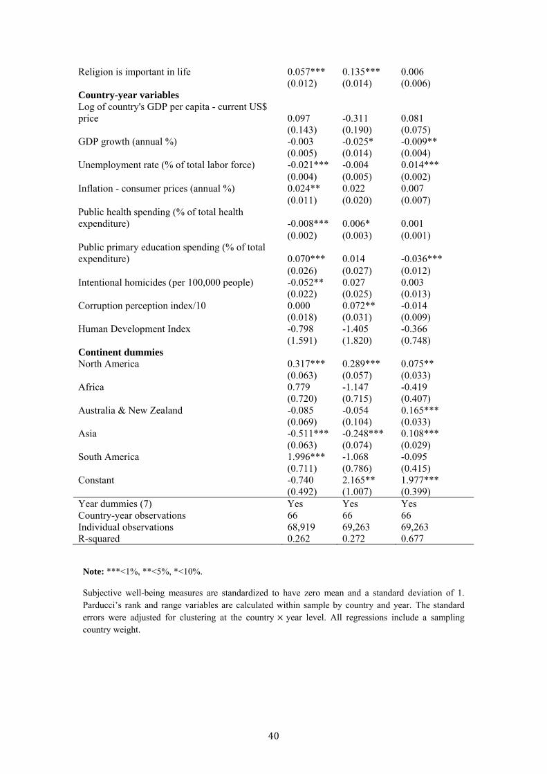
Religion is important in life 0.057*** 0.135*** 0.006 (0.012) (0.014) (0.006)
Country-year variables Log of country's GDP per capita - current US$ price 0.097 -0.311 0.081
(0.143) (0.190) (0.075) GDP growth (annual %) -0.003 -0.025* -0.009** (0.005) (0.014) (0.004) Unemployment rate (% of total labor force) -0.021*** -0.004 0.014***
(0.004) (0.005) (0.002) Inflation - consumer prices (annual %) 0.024** 0.022 0.007
(0.011) (0.020) (0.007) Public health spending (% of total health expenditure) -0.008*** 0.006* 0.001
(0.002) (0.003) (0.001) Public primary education spending (% of total expenditure) 0.070*** 0.014 -0.036***
(0.026) (0.027) (0.012) Intentional homicides (per 100,000 people) -0.052** 0.027 0.003
(0.022) (0.025) (0.013) Corruption perception index/10 0.000 0.072** -0.014
(0.018) (0.031) (0.009) Human Development Index -0.798 -1.405 -0.366
(1.591) (1.820) (0.748) Continent dummies North America 0.317*** 0.289*** 0.075**
(0.063) (0.057) (0.033) Africa 0.779 -1.147 -0.419
(0.720) (0.715) (0.407) Australia & New Zealand -0.085 -0.054 0.165***
(0.069) (0.104) (0.033) Asia -0.511*** -0.248*** 0.108***
(0.063) (0.074) (0.029) South America 1.996*** -1.068 -0.095
(0.711) (0.786) (0.415) Constant -0.740 2.165** 1.977***
(0.492) (1.007) (0.399) Year dummies (7) Yes Yes Yes Country-year observations 66 66 66 Individual observations 68,919 69,263 69,263 R-squared 0.262 0.272 0.677
Note: ***<1%, **<5%, *<10%.
Subjective well-being measures are standardized to have zero mean and a standard deviation of 1. Parducci’s rank and range variables are calculated within sample by country and year. The standard errors were adjusted for clustering at the country year level. All regressions include a sampling country weight.
41
Table 2: Country Fixed Effects – Sub-sample Regressions by Continents
VARIABLES All Europe
North America
Asia Africa +
South America
Australia + NZ
A) Cantril Life Ladder Share of taxable income held by the top 1 percent 0.044** -0.044** -0.020 -0.004 0.645*** 0.148***
(0.020) (0.022) (0.112) (0.154) (0.159) (0.015)Log of household income per capita - 2010 PPP 0.034 -0.044 -0.051 -0.064 0.023 0.269**
(0.032) (0.031) (0.053) (0.127) (0.143) (0.067)Log(relative household income) 0.065** -0.001 -0.043 0.080 0.039 -0.011
(0.027) (0.032) (0.084) (0.066) (0.070) (0.070)Parducci’s within-sample rank variable 0.290*** 0.317*** 0.254 0.354*** 0.592** -0.000
(0.059) (0.069) (0.191) (0.105) (0.250) (0.266)Parducci’s within-sample range variable 0.241 0.595** 0.945 0.912 0.395 -0.845***
(0.212) (0.258) (0.621) (0.927) (1.126) (0.130)
B) Positive Emotional Experiences Share of taxable income held by the top 1 percent 0.056* 0.012 0.020 0.152 0.227* 0.054 (0.030) (0.023) (0.105) (0.125) (0.114) (0.052)Log of household income per capita - 2010 PPP 0.011 0.017 0.075 0.007 0.286 0.020
(0.026) (0.029) (0.083) (0.093) (0.156) (0.048)Log(relative household income) 0.030 0.034 -0.142* 0.034 0.018 0.111*
(0.024) (0.029) (0.065) (0.062) (0.038) (0.049)Parducci’s within-sample rank variable 0.111** 0.163*** -0.056 0.095 -0.048 -0.168
(0.044) (0.049) (0.078) (0.128) (0.166) (0.231)Parducci’s within-sample range variable -0.070 -0.257 -0.312 0.032 -1.725 0.333
(0.193) (0.185) (0.605) (0.650) (1.207) (0.497)
C) Negative Emotional Experiences
42
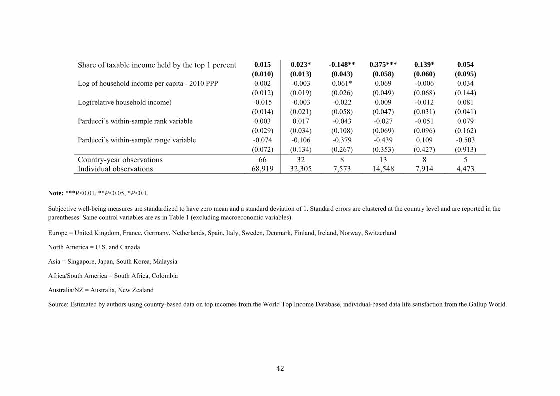
Share of taxable income held by the top 1 percent 0.015 0.023* -0.148** 0.375*** 0.139* 0.054 (0.010) (0.013) (0.043) (0.058) (0.060) (0.095)Log of household income per capita - 2010 PPP 0.002 -0.003 0.061* 0.069 -0.006 0.034 (0.012) (0.019) (0.026) (0.049) (0.068) (0.144)Log(relative household income) -0.015 -0.003 -0.022 0.009 -0.012 0.081 (0.014) (0.021) (0.058) (0.047) (0.031) (0.041)Parducci’s within-sample rank variable 0.003 0.017 -0.043 -0.027 -0.051 0.079 (0.029) (0.034) (0.108) (0.069) (0.096) (0.162)Parducci’s within-sample range variable -0.074 -0.106 -0.379 -0.439 0.109 -0.503 (0.072) (0.134) (0.267) (0.353) (0.427) (0.913)
Country-year observations 66 32 8 13 8 5Individual observations 68,919 32,305 7,573 14,548 7,914 4,473
Note: ***P<0.01, **P<0.05, *P<0.1.
Subjective well-being measures are standardized to have zero mean and a standard deviation of 1. Standard errors are clustered at the country level and are reported in the parentheses. Same control variables are as in Table 1 (excluding macroeconomic variables).
Europe = United Kingdom, France, Germany, Netherlands, Spain, Italy, Sweden, Denmark, Finland, Ireland, Norway, Switzerland
North America = U.S. and Canada
Asia = Singapore, Japan, South Korea, Malaysia
Africa/South America = South Africa, Colombia
Australia/NZ = Australia, New Zealand
Source: Estimated by authors using country-based data on top incomes from the World Top Income Database, individual-based data life satisfaction from the Gallup World.
43
Table 3: Life Evaluation, Positive, and Negative Emotional Well-being Equations with Country Fixed Effects – European Sample
A) Females B) Males
VARIABLES Life
evaluation Positive
experience Negative
experience Life
evaluation Positive
experience Negative
experience Share of taxable income held by the top 1 percent -0.045* 0.023 0.026 -0.044* -0.005 0.021
(0.023) (0.021) (0.020) (0.024) (0.035) (0.013) Observations 18,767 18,889 18,889 13,538 13,597 13,597 R-squared 0.244 0.301 0.692 0.231 0.233 0.653 C) Age<=40 D) Age>40
VARIABLES Life
evaluation Positive
experience Negative
experience Life
evaluation Positive
experience Negative
experience Share of taxable income held by the top 1 percent -0.079*** -0.032 0.083*** -0.013 0.035 -0.019
(0.025) (0.031) (0.014) (0.028) (0.023) (0.016) Observations 10,105 10,129 10,129 22,200 22,357 22,357 R-squared 0.202 0.282 0.653 0.260 0.267 0.698
E) High
school/college F) Less than high
school/college
VARIABLES Life
evaluationPositive
experienceNegative
experienceLife
evaluationPositive
experienceNegative
experience Share of taxable income held by the top 1 percent -0.007 0.010 0.012 -0.056** 0.015 0.022
(0.021) (0.020) (0.018) (0.024) (0.026) (0.013) Individual observations 8,276 8,310 8,310 23,752 23,888 23,888 R-squared 0.186 0.244 0.644 0.237 0.271 0.685
Note: ***<1%, **<5%, *<10%. Subjective well-being measures are standardized to have zero mean and a standard deviation of 1. The standard errors were adjusted for clustering at the country year level. Country-year observations = 32. Control variables are as in Table 1.
44
Table 4: Life Evaluation, Positive, and Negative Emotional Well-being Equations with Country Fixed Effects and Interactions Between Top Income Shares and Household Income: European Sample, 2006-2012
(1) (2) (3) (4) (5) (6)
VARIABLES Life evaluation
Positive experience
Negative experience
Life evaluation
Positive experience
Negative experience
Share of taxable income held by the top 1 percent -0.090*** -0.011 0.040* (0.030) (0.028) (0.023)
Log of household income per capita - 2010 PPP -0.094** -0.008 0.015 -0.074* 0.007 0.009 (0.037) (0.033) (0.023) (0.038) (0.026) (0.020)
Log(relative household income) 0.001 0.035 -0.003 0.001 0.035 -0.003 (0.031) (0.029) (0.021) (0.031) (0.029) (0.021) Parducci’s within-sample rank variable 0.322*** 0.165*** 0.016 0.311*** 0.167*** 0.021 (0.070) (0.050) (0.034) (0.073) (0.049) (0.035) Parducci’s within-sample range variable 0.616** -0.247 -0.114 0.541** -0.259 -0.077 (0.256) (0.172) (0.134) (0.230) (0.172) (0.116) Interaction effect Top 1 percent income share log(household income per capita) 0.005** 0.002 -0.002
(0.002) (0.002) (0.002) Share 8%-12% dummy log(household income per capita) 0.069*** 0.009 -0.034**
(0.022) (0.018) (0.014) Share more than 12% dummy log(household income per capita) 0.057*** 0.027** -0.022**
(0.014) (0.012) (0.009) Individual observations 32,305 32,486 32,486 32,305 32,486 32,486 R-squared 0.235 0.269 0.678 0.236 0.269 0.678 Note: ***<1%, **<5%, *<10%. Subjective well-being measures are standardized to have zero mean and a standard deviation of 1. The standard errors were adjusted for clustering at the country year level. Country-year observations = 32. Control variables are as in Table 1.
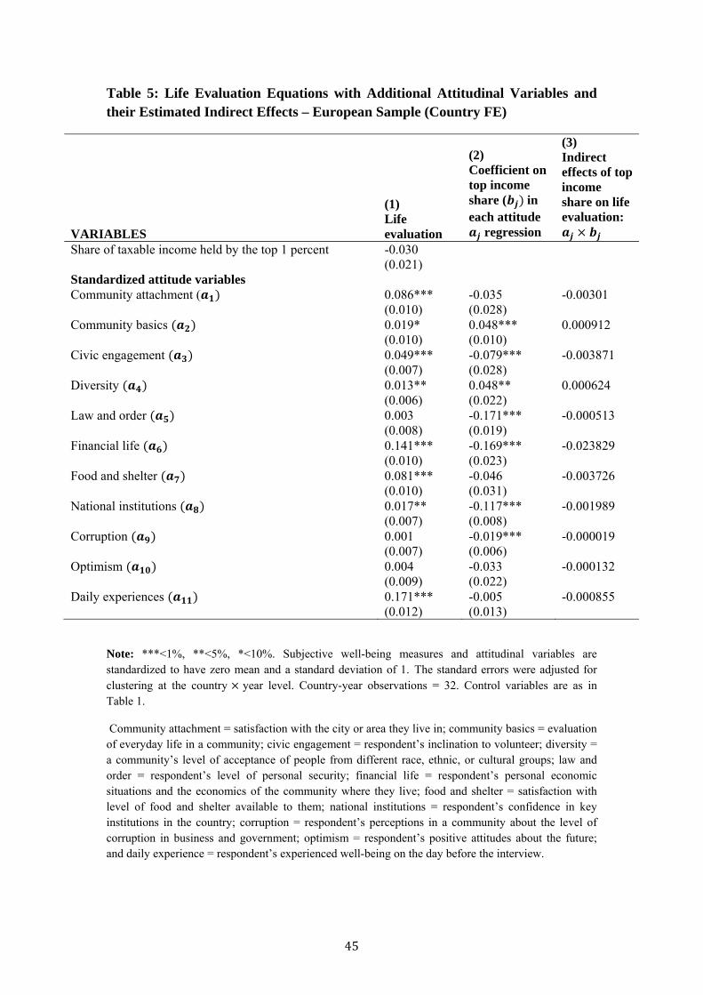
45
Table 5: Life Evaluation Equations with Additional Attitudinal Variables and their Estimated Indirect Effects – European Sample (Country FE)
VARIABLES
(1) Life evaluation
(2) Coefficient on top income share ( in each attitude
regression
(3) Indirect effects of top income share on life evaluation:
Share of taxable income held by the top 1 percent -0.030
(0.021) Standardized attitude variables Community attachment ( 0.086*** -0.035 -0.00301
(0.010) (0.028) Community basics 0.019* 0.048*** 0.000912
(0.010) (0.010) Civic engagement 0.049*** -0.079*** -0.003871
(0.007) (0.028) Diversity 0.013** 0.048** 0.000624
(0.006) (0.022) Law and order 0.003 -0.171*** -0.000513
(0.008) (0.019) Financial life 0.141*** -0.169*** -0.023829
(0.010) (0.023) Food and shelter 0.081*** -0.046 -0.003726
(0.010) (0.031) National institutions 0.017** -0.117*** -0.001989
(0.007) (0.008) Corruption 0.001 -0.019*** -0.000019
(0.007) (0.006) Optimism 0.004 -0.033 -0.000132
(0.009) (0.022) Daily experiences 0.171*** -0.005 -0.000855 (0.012) (0.013)
Note: ***<1%, **<5%, *<10%. Subjective well-being measures and attitudinal variables are standardized to have zero mean and a standard deviation of 1. The standard errors were adjusted for clustering at the country year level. Country-year observations = 32. Control variables are as in Table 1.
Community attachment = satisfaction with the city or area they live in; community basics = evaluation of everyday life in a community; civic engagement = respondent’s inclination to volunteer; diversity = a community’s level of acceptance of people from different race, ethnic, or cultural groups; law and order = respondent’s level of personal security; financial life = respondent’s personal economic situations and the economics of the community where they live; food and shelter = satisfaction with level of food and shelter available to them; national institutions = respondent’s confidence in key institutions in the country; corruption = respondent’s perceptions in a community about the level of corruption in business and government; optimism = respondent’s positive attitudes about the future; and daily experience = respondent’s experienced well-being on the day before the interview.
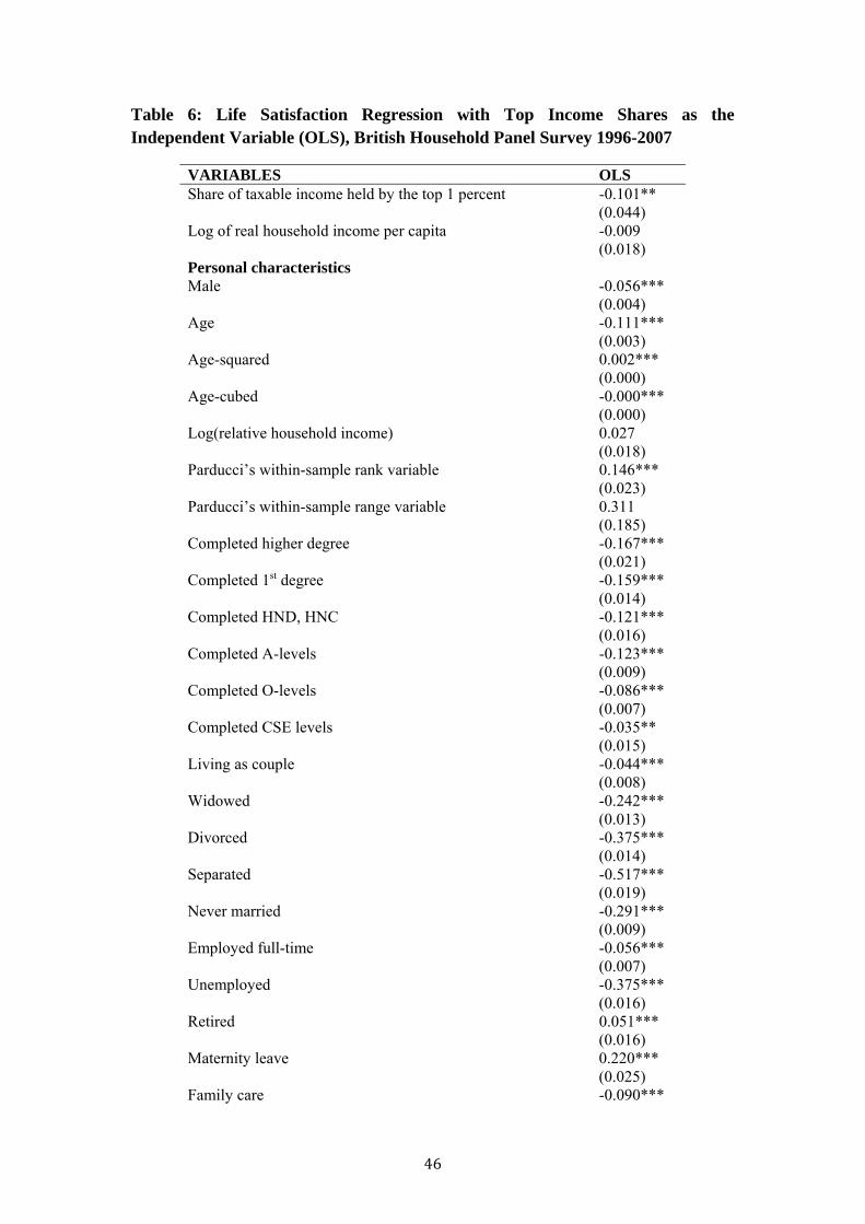
46
Table 6: Life Satisfaction Regression with Top Income Shares as the Independent Variable (OLS), British Household Panel Survey 1996-2007
VARIABLES OLS Share of taxable income held by the top 1 percent -0.101**
(0.044) Log of real household income per capita -0.009
(0.018) Personal characteristics Male -0.056***
(0.004) Age -0.111***
(0.003) Age-squared 0.002***
(0.000) Age-cubed -0.000***
(0.000) Log(relative household income) 0.027 (0.018) Parducci’s within-sample rank variable 0.146*** (0.023) Parducci’s within-sample range variable 0.311 (0.185) Completed higher degree -0.167***
(0.021) Completed 1st degree -0.159***
(0.014) Completed HND, HNC -0.121***
(0.016) Completed A-levels -0.123***
(0.009) Completed O-levels -0.086***
(0.007) Completed CSE levels -0.035**
(0.015) Living as couple -0.044***
(0.008) Widowed -0.242***
(0.013) Divorced -0.375***
(0.014) Separated -0.517***
(0.019) Never married -0.291***
(0.009) Employed full-time -0.056***
(0.007) Unemployed -0.375***
(0.016) Retired 0.051***
(0.016) Maternity leave 0.220***
(0.025) Family care -0.090***
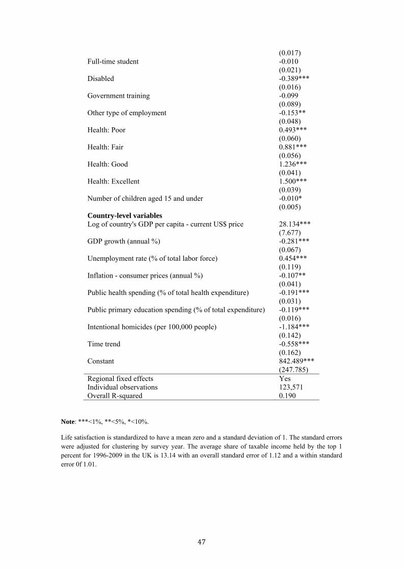
47
(0.017) Full-time student -0.010
(0.021) Disabled -0.389***
(0.016) Government training -0.099
(0.089) Other type of employment -0.153**
(0.048) Health: Poor 0.493***
(0.060) Health: Fair 0.881***
(0.056) Health: Good 1.236***
(0.041) Health: Excellent 1.500***
(0.039) Number of children aged 15 and under -0.010*
(0.005) Country-level variables Log of country's GDP per capita - current US$ price 28.134***
(7.677) GDP growth (annual %) -0.281*** (0.067) Unemployment rate (% of total labor force) 0.454*** (0.119) Inflation - consumer prices (annual %) -0.107**
(0.041) Public health spending (% of total health expenditure) -0.191***
(0.031) Public primary education spending (% of total expenditure) -0.119***
(0.016) Intentional homicides (per 100,000 people) -1.184***
(0.142) Time trend -0.558*** (0.162) Constant 842.489***
(247.785) Regional fixed effects Yes Individual observations 123,571 Overall R-squared 0.190
Note: ***<1%, **<5%, *<10%.
Life satisfaction is standardized to have a mean zero and a standard deviation of 1. The standard errors were adjusted for clustering by survey year. The average share of taxable income held by the top 1 percent for 1996-2009 in the UK is 13.14 with an overall standard error of 1.12 and a within standard error 0f 1.01.
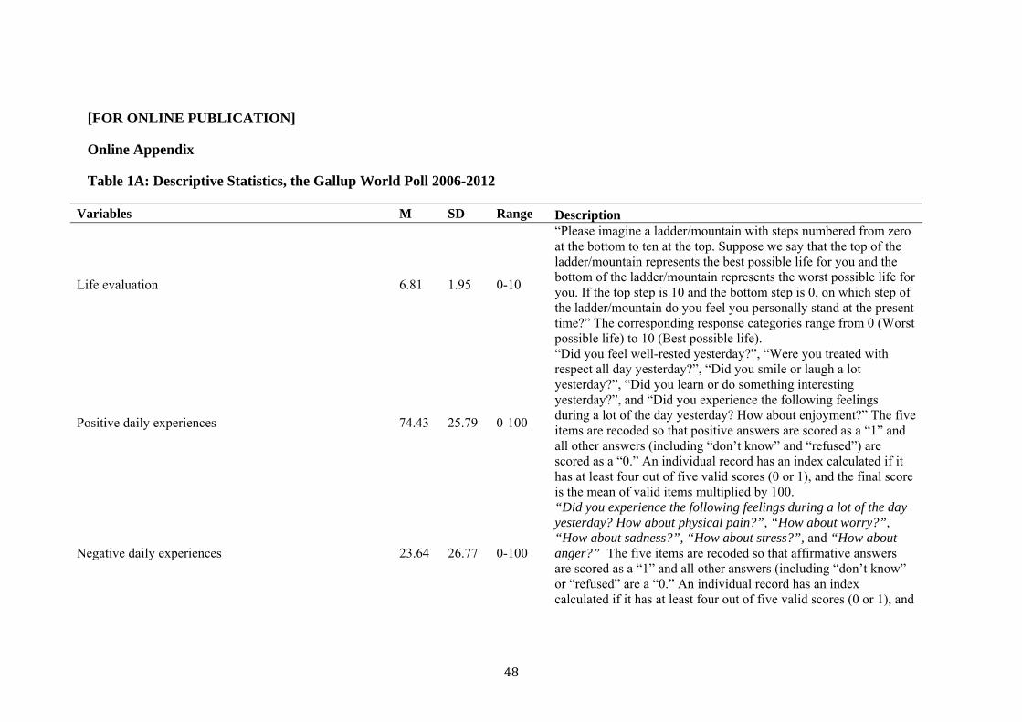
48
[FOR ONLINE PUBLICATION]
Online Appendix
Table 1A: Descriptive Statistics, the Gallup World Poll 2006-2012
Variables M SD Range Description
Life evaluation 6.81 1.95 0-10
“Please imagine a ladder/mountain with steps numbered from zero at the bottom to ten at the top. Suppose we say that the top of the ladder/mountain represents the best possible life for you and the bottom of the ladder/mountain represents the worst possible life for you. If the top step is 10 and the bottom step is 0, on which step of the ladder/mountain do you feel you personally stand at the present time?” The corresponding response categories range from 0 (Worst possible life) to 10 (Best possible life).
Positive daily experiences 74.43 25.79 0-100
“Did you feel well-rested yesterday?”, “Were you treated with respect all day yesterday?”, “Did you smile or laugh a lot yesterday?”, “Did you learn or do something interesting yesterday?”, and “Did you experience the following feelings during a lot of the day yesterday? How about enjoyment?” The five items are recoded so that positive answers are scored as a “1” and all other answers (including “don’t know” and “refused”) are scored as a “0.” An individual record has an index calculated if it has at least four out of five valid scores (0 or 1), and the final score is the mean of valid items multiplied by 100.
Negative daily experiences 23.64 26.77 0-100
“Did you experience the following feelings during a lot of the day yesterday? How about physical pain?”, “How about worry?”, “How about sadness?”, “How about stress?”, and “How about anger?” The five items are recoded so that affirmative answers are scored as a “1” and all other answers (including “don’t know” or “refused” are a “0.” An individual record has an index calculated if it has at least four out of five valid scores (0 or 1), and
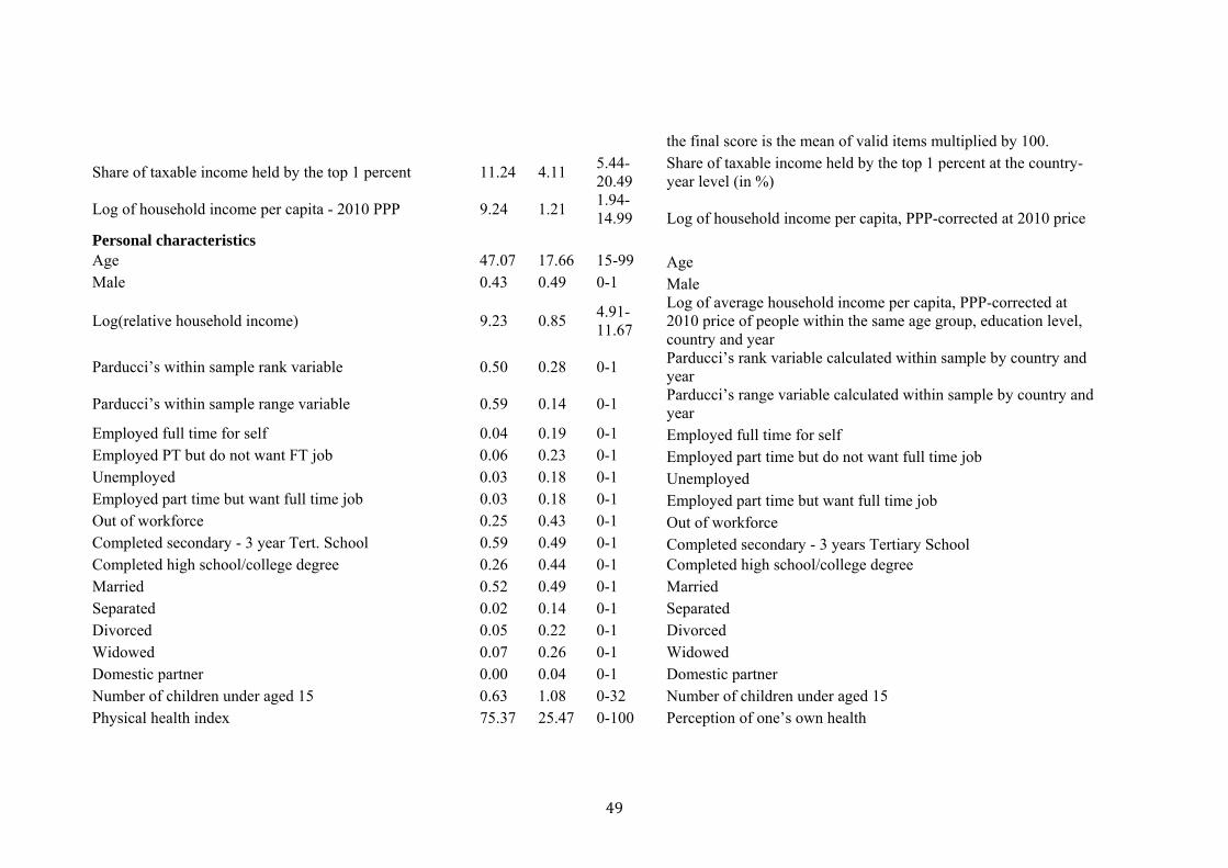
49
the final score is the mean of valid items multiplied by 100.
Share of taxable income held by the top 1 percent 11.24 4.11 5.44-20.49
Share of taxable income held by the top 1 percent at the country-year level (in %)
Log of household income per capita - 2010 PPP 9.24 1.21 1.94-14.99 Log of household income per capita, PPP-corrected at 2010 price
Personal characteristics Age 47.07 17.66 15-99 Age Male 0.43 0.49 0-1 Male
Log(relative household income) 9.23 0.85 4.91-11.67
Log of average household income per capita, PPP-corrected at 2010 price of people within the same age group, education level, country and year
Parducci’s within sample rank variable 0.50 0.28 0-1 Parducci’s rank variable calculated within sample by country and year
Parducci’s within sample range variable 0.59 0.14 0-1 Parducci’s range variable calculated within sample by country and year
Employed full time for self 0.04 0.19 0-1 Employed full time for self Employed PT but do not want FT job 0.06 0.23 0-1 Employed part time but do not want full time job Unemployed 0.03 0.18 0-1 Unemployed Employed part time but want full time job 0.03 0.18 0-1 Employed part time but want full time job Out of workforce 0.25 0.43 0-1 Out of workforce Completed secondary - 3 year Tert. School 0.59 0.49 0-1 Completed secondary - 3 years Tertiary School Completed high school/college degree 0.26 0.44 0-1 Completed high school/college degree Married 0.52 0.49 0-1 Married Separated 0.02 0.14 0-1 Separated Divorced 0.05 0.22 0-1 Divorced Widowed 0.07 0.26 0-1 Widowed Domestic partner 0.00 0.04 0-1 Domestic partner Number of children under aged 15 0.63 1.08 0-32 Number of children under aged 15 Physical health index 75.37 25.47 0-100 Perception of one’s own health
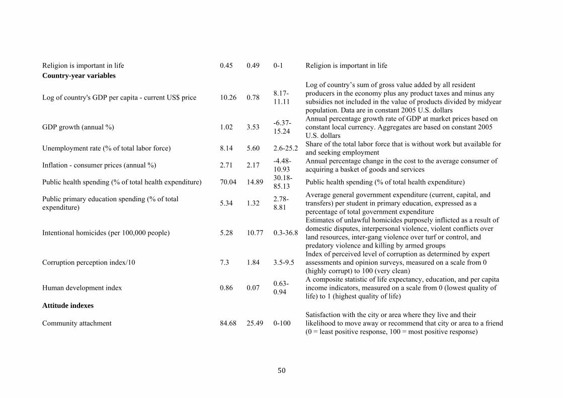
50
Religion is important in life 0.45 0.49 0-1 Religion is important in life Country-year variables
Log of country's GDP per capita - current US$ price 10.26 0.78 8.17-11.11
Log of country’s sum of gross value added by all resident producers in the economy plus any product taxes and minus any subsidies not included in the value of products divided by midyear population. Data are in constant 2005 U.S. dollars
GDP growth (annual %) 1.02 3.53 -6.37-15.24
Annual percentage growth rate of GDP at market prices based on constant local currency. Aggregates are based on constant 2005 U.S. dollars
Unemployment rate (% of total labor force) 8.14 5.60 2.6-25.2 Share of the total labor force that is without work but available for and seeking employment
Inflation - consumer prices (annual %) 2.71 2.17 -4.48-10.93
Annual percentage change in the cost to the average consumer of acquiring a basket of goods and services
Public health spending (% of total health expenditure) 70.04 14.89 30.18-85.13
Public health spending (% of total health expenditure)
Public primary education spending (% of total expenditure)
5.34 1.32 2.78-8.81
Average general government expenditure (current, capital, and transfers) per student in primary education, expressed as a percentage of total government expenditure
Intentional homicides (per 100,000 people) 5.28 10.77 0.3-36.8
Estimates of unlawful homicides purposely inflicted as a result of domestic disputes, interpersonal violence, violent conflicts over land resources, inter-gang violence over turf or control, and predatory violence and killing by armed groups
Corruption perception index/10 7.3 1.84 3.5-9.5 Index of perceived level of corruption as determined by expert assessments and opinion surveys, measured on a scale from 0 (highly corrupt) to 100 (very clean)
Human development index 0.86 0.07 0.63-0.94
A composite statistic of life expectancy, education, and per capita income indicators, measured on a scale from 0 (lowest quality of life) to 1 (highest quality of life)
Attitude indexes
Community attachment 84.68 25.49 0-100 Satisfaction with the city or area where they live and their likelihood to move away or recommend that city or area to a friend (0 = least positive response, 100 = most positive response)
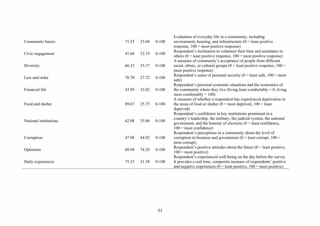
51
Community basics 71.53 23.04 0-100 Evaluation of everyday life in a community, including environment, housing, and infrastructure (0 = least positive response, 100 = most positive response)
Civic engagement 41.66 32.19 0-100 Respondent’s inclination to volunteer their time and assistance to others (0 = least positive response, 100 = most positive response)
Diversity 66.32 35.37 0-100 A measure of community’s acceptance of people from different racial, ethnic, or cultural groups (0 = least positive response, 100 = most positive response)
Law and order 76.70 27.72 0-100 Respondent’s sense of personal security (0 = least safe, 100 = most safe)
Financial life 43.95 32.02 0-100 Respondent’s personal economic situations and the economics of the community where they live (living least comfortably = 0, living most comfortably = 100)
Food and shelter 89.67 25.75 0-100 A measure of whether a respondent has experienced deprivation in the areas of food or shelter (0 = most deprived, 100 = least deprived)
National institutions 62.88 33.06 0-100
Respondent’s confidence in key institutions prominent in a country’s leadership: the military, the judicial system, the national government, and the honesty of elections (0 = least confidence, 100 = most confidence)
Corruption 47.98 44.92 0-100 Respondent’s perceptions in a community about the level of corruption in business and government (0 = least corrupt, 100 = most corrupt)
Optimism 68.94 74.28 0-100 Respondent’s positive attitudes about the future (0 = least positive, 100 = most positive)
Daily experiences 75.23 21.58 0-100 Respondent’s experienced well-being on the day before the survey It provides a real time, composite measure of respondents’ positive and negative experiences (0 = least positive, 100 = most positive)
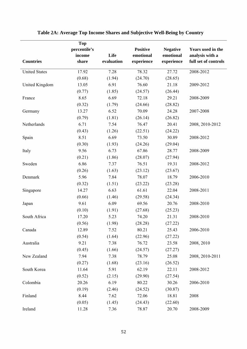
52
Table 2A: Average Top Income Shares and Subjective Well-Being by Country
Countries
Top percentile’s
income share
Life evaluation
Positive emotional experience
Negative emotional experience
Years used in the analysis with a full set of controls
United States 17.92 7.28 78.32 27.72 2008-2012
(0.68) (1.94) (24.70) (28.65)
United Kingdom 13.05 6.91 76.60 21.18 2009-2012
(0.77) (1.85) (24.57) (26.44)
France 8.65 6.69 72.18 29.21 2008-2009
(0.32) (1.79) (24.66) (28.82)
Germany 13.27 6.52 70.09 24.28 2007-2008
(0.79) (1.81) (26.14) (26.82)
Netherlands 6.71 7.54 76.47 20.41 2008, 2010-2012
(0.43) (1.26) (22.51) (24.22)
Spain 8.51 6.69 73.50 30.89 2008-2012
(0.30) (1.93) (24.26) (29.04)
Italy 9.56 6.73 67.86 28.77 2008-2009
(0.21) (1.86) (28.07) (27.94)
Sweden 6.86 7.37 76.51 19.31 2008-2012
(0.26) (1.63) (23.12) (23.67)
Denmark 5.96 7.84 78.07 18.79 2006-2010
(0.32) (1.51) (23.22) (23.28)
Singapore 14.27 6.63 61.61 22.04 2008-2011
(0.66) (1.46) (29.58) (24.34)
Japan 9.61 6.09 69.56 20.76 2008-2010
(0.10) (1.91) (27.68) (25.23)
South Africa 17.20 5.23 74.20 21.31 2008-2010
(0.56) (1.98) (28.28) (27.22)
Canada 12.89 7.52 80.21 25.43 2006-2010
(0.54) (1.64) (22.96) (27.22)
Australia 9.21 7.38 76.72 23.58 2008, 2010
(0.45) (1.66) (24.57) (27.27)
New Zealand 7.94 7.38 78.79 25.08 2008, 2010-2011
(0.27) (1.68) (23.16) (26.52)
South Korea 11.64 5.91 62.19 22.11 2008-2012
(0.52) (2.15) (29.90) (27.54)
Colombia 20.26 6.19 80.22 30.26 2006-2010
(0.19) (2.46) (24.52) (30.87)
Finland 8.44 7.62 72.06 18.81 2008
(0.05) (1.45) (24.43) (22.60)
Ireland 11.28 7.36 78.87 20.70 2008-2009
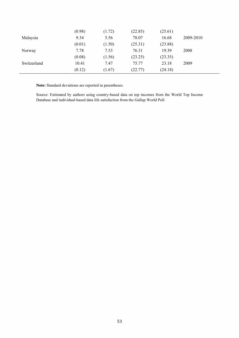
53
(0.98) (1.72) (22.85) (25.61)
Malaysia 9.34 5.56 78.07 16.68 2009-2010
(0.01) (1.50) (25.31) (23.88)
Norway 7.78 7.53 76.31 19.39 2008
(0.08) (1.56) (23.25) (23.35)
Switzerland 10.41 7.47 75.77 23.18 2009
(0.12) (1.67) (22.77) (24.18)
Note: Standard deviations are reported in parentheses.
Source: Estimated by authors using country-based data on top incomes from the World Top Income Database and individual-based data life satisfaction from the Gallup World Poll.
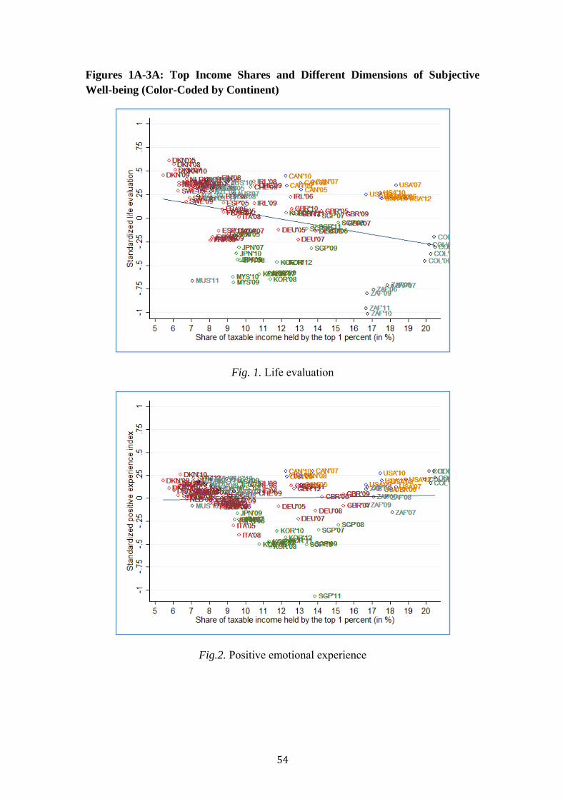
54
Figures 1A-3A: Top Income Shares and Different Dimensions of Subjective Well-being (Color-Coded by Continent)
Fig. 1. Life evaluation
Fig.2. Positive emotional experience
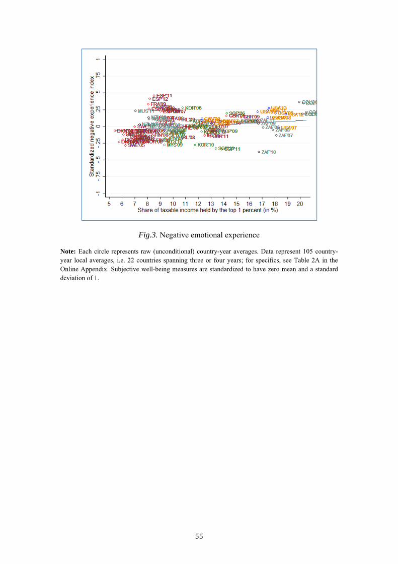
55
Fig.3. Negative emotional experience
Note: Each circle represents raw (unconditional) country-year averages. Data represent 105 country-year local averages, i.e. 22 countries spanning three or four years; for specifics, see Table 2A in the Online Appendix. Subjective well-being measures are standardized to have zero mean and a standard deviation of 1.
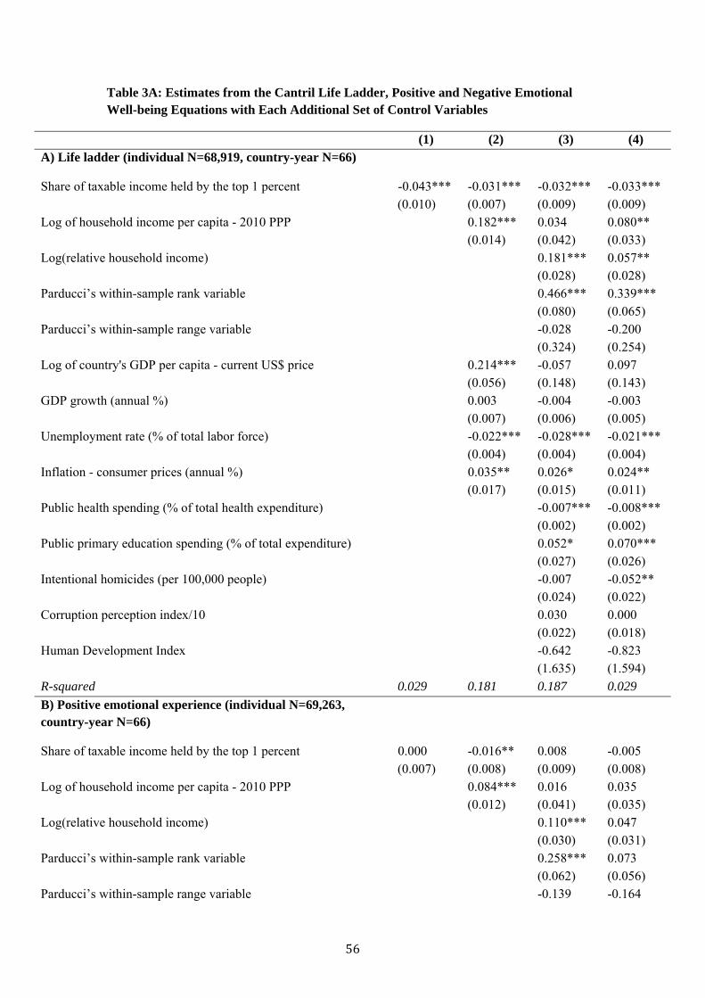
56
Table 3A: Estimates from the Cantril Life Ladder, Positive and Negative Emotional Well-being Equations with Each Additional Set of Control Variables
(1) (2) (3) (4) A) Life ladder (individual N=68,919, country-year N=66)
Share of taxable income held by the top 1 percent -0.043*** -0.031*** -0.032*** -0.033*** (0.010) (0.007) (0.009) (0.009)
Log of household income per capita - 2010 PPP 0.182*** 0.034 0.080** (0.014) (0.042) (0.033)
Log(relative household income) 0.181*** 0.057** (0.028) (0.028) Parducci’s within-sample rank variable 0.466*** 0.339*** (0.080) (0.065) Parducci’s within-sample range variable -0.028 -0.200 (0.324) (0.254) Log of country's GDP per capita - current US$ price 0.214*** -0.057 0.097 (0.056) (0.148) (0.143) GDP growth (annual %) 0.003 -0.004 -0.003 (0.007) (0.006) (0.005) Unemployment rate (% of total labor force) -0.022*** -0.028*** -0.021*** (0.004) (0.004) (0.004) Inflation - consumer prices (annual %) 0.035** 0.026* 0.024** (0.017) (0.015) (0.011) Public health spending (% of total health expenditure) -0.007*** -0.008*** (0.002) (0.002) Public primary education spending (% of total expenditure) 0.052* 0.070*** (0.027) (0.026) Intentional homicides (per 100,000 people) -0.007 -0.052** (0.024) (0.022) Corruption perception index/10 0.030 0.000 (0.022) (0.018) Human Development Index -0.642 -0.823 (1.635) (1.594) R-squared 0.029 0.181 0.187 0.029
B) Positive emotional experience (individual N=69,263, country-year N=66)
Share of taxable income held by the top 1 percent 0.000 -0.016** 0.008 -0.005 (0.007) (0.008) (0.009) (0.008)
Log of household income per capita - 2010 PPP 0.084*** 0.016 0.035 (0.012) (0.041) (0.035)
Log(relative household income) 0.110*** 0.047 (0.030) (0.031) Parducci’s within-sample rank variable 0.258*** 0.073 (0.062) (0.056) Parducci’s within-sample range variable -0.139 -0.164
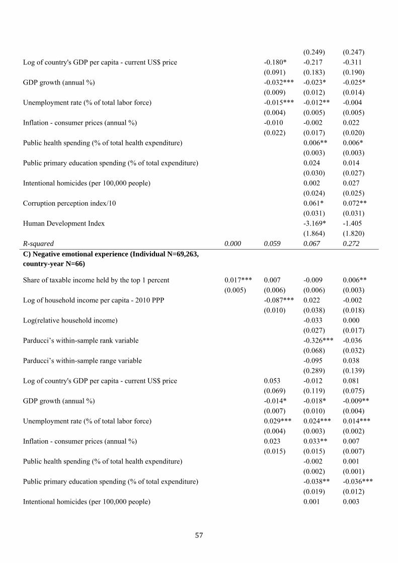
57
(0.249) (0.247) Log of country's GDP per capita - current US$ price -0.180* -0.217 -0.311 (0.091) (0.183) (0.190) GDP growth (annual %) -0.032*** -0.023* -0.025* (0.009) (0.012) (0.014) Unemployment rate (% of total labor force) -0.015*** -0.012** -0.004 (0.004) (0.005) (0.005) Inflation - consumer prices (annual %) -0.010 -0.002 0.022 (0.022) (0.017) (0.020) Public health spending (% of total health expenditure) 0.006** 0.006* (0.003) (0.003) Public primary education spending (% of total expenditure) 0.024 0.014 (0.030) (0.027) Intentional homicides (per 100,000 people) 0.002 0.027 (0.024) (0.025) Corruption perception index/10 0.061* 0.072** (0.031) (0.031) Human Development Index -3.169* -1.405 (1.864) (1.820) R-squared 0.000 0.059 0.067 0.272
C) Negative emotional experience (Individual N=69,263, country-year N=66)
Share of taxable income held by the top 1 percent 0.017*** 0.007 -0.009 0.006** (0.005) (0.006) (0.006) (0.003)
Log of household income per capita - 2010 PPP -0.087*** 0.022 -0.002 (0.010) (0.038) (0.018) Log(relative household income) -0.033 0.000 (0.027) (0.017) Parducci’s within-sample rank variable -0.326*** -0.036 (0.068) (0.032) Parducci’s within-sample range variable -0.095 0.038 (0.289) (0.139) Log of country's GDP per capita - current US$ price 0.053 -0.012 0.081 (0.069) (0.119) (0.075) GDP growth (annual %) -0.014* -0.018* -0.009** (0.007) (0.010) (0.004) Unemployment rate (% of total labor force) 0.029*** 0.024*** 0.014*** (0.004) (0.003) (0.002) Inflation - consumer prices (annual %) 0.023 0.033** 0.007 (0.015) (0.015) (0.007) Public health spending (% of total health expenditure) -0.002 0.001 (0.002) (0.001) Public primary education spending (% of total expenditure) -0.038** -0.036*** (0.019) (0.012) Intentional homicides (per 100,000 people) 0.001 0.003
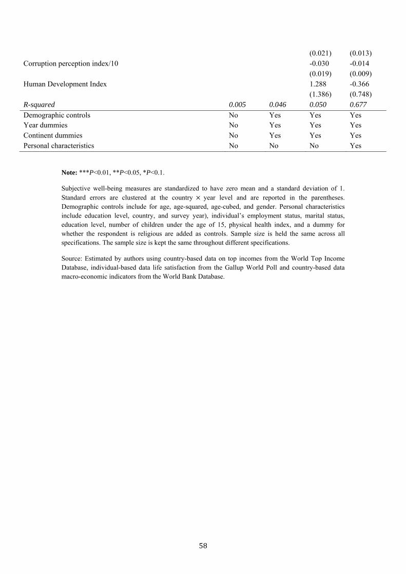
58
(0.021) (0.013) Corruption perception index/10 -0.030 -0.014 (0.019) (0.009) Human Development Index 1.288 -0.366 (1.386) (0.748) R-squared 0.005 0.046 0.050 0.677
Demographic controls No Yes Yes Yes Year dummies No Yes Yes Yes Continent dummies No Yes Yes Yes Personal characteristics No No No Yes
Note: ***P<0.01, **P<0.05, *P<0.1.
Subjective well-being measures are standardized to have zero mean and a standard deviation of 1. Standard errors are clustered at the country year level and are reported in the parentheses. Demographic controls include for age, age-squared, age-cubed, and gender. Personal characteristics include education level, country, and survey year), individual’s employment status, marital status, education level, number of children under the age of 15, physical health index, and a dummy for whether the respondent is religious are added as controls. Sample size is held the same across all specifications. The sample size is kept the same throughout different specifications.
Source: Estimated by authors using country-based data on top incomes from the World Top Income Database, individual-based data life satisfaction from the Gallup World Poll and country-based data macro-economic indicators from the World Bank Database.
![Pushing and Being Pulled Around the Postmodern Turn · Pushing and Being Pulled Around the Postmodern Turn [M]ethodology embraces the entire scientific quest and not merely some selected](https://img.pdfslide.net/doc/110x75/5e9c714aa8c92a04b114c84e/pushing-and-being-pulled-around-the-postmodern-turn-pushing-and-being-pulled-around.jpg)