Topic 11: The Central Limit Theoremjwatkins/k-clt.pdf · Topic 11: The Central Limit Theorem October 11 and 18, 2011 1 Introduction In the discussion leading to the law of large numbers,

Topic 11: The Central Limit Theorem∗

October 11 and 18, 2011

1 IntroductionIn the discussion leading to the law of large numbers, we saw visually that the sample means converges to the distri-butional mean. In symbols,

Xn → µ as n→∞.

Using the Pythagorean theorem for independent random variables, we obtained the more precise statement that thestandard deviation of Xn is inversely proportional to

√n, the square root of the number of observations. For example,

for simulations based on observations of independent random variables, uniformly distributed on [0, 1], we see, asanticipated, the running averages converging to

µ =∫ 1

0

xfX(x) dx =∫ 1

0

x dx =x2

2

∣∣∣10

=12,

the distributional mean.Now, we zoom around the mean value of µ = 1/2. Because the standard deviation σXn

∝ 1/√n, we magnify the

difference between the running average and the mean by a factor of√n and investigate the graph of

√n

(1nSn − µ

)versus n. The results of a simulation are displayed in Figure 1.

As we see in Figure 2, even if we extend this simulation for larger values of n, we continue to see fluctuationsabout the center of roughly the same size and the size of the fluctuations for a single realization of a simulation cannotbe predicted in advance.

Thus, we focus on addressing a broader question: Does the distribution of the size of these fluctuations have anyregular and predictable structure? This question and the investigation that led to led to its answer, the central limittheorem, constitute one of the most important episodes in mathematics.

2 The Classical Central Limit TheoremLet’s begin by examining the distribution for the sum ofX1, X2 . . . Xn, independent and identically distributed randomvariables

Sn = X1 +X2 + · · ·+Xn,

what distribution do we see? Let’s look first to the simplest case, Xi Bernoulli random variables. In this case, the sumSn is a binomial random variable. We look at two cases - in the first we keep the number of trials the same at n = 100and vary the success probability p. In the second case, we keep the success probability the same at p = 1/2, but varythe number of trials.∗ c© 2011 Joseph C. Watkins

139

Introduction to Statistical Methodology The Central Limit Theorem

0 50 100 150 200

0.3

0.4

0.5

0.6

0.7

n

s/n

0 50 100 150 200

-0.3

-0.2

-0.1

0.0

0.1

0.2

0.3

n(s

- n

/2)/

sqrt

(n)

Figure 1: a. Running average of independent random variables, uniform on [0, 1]. b. Running average centered at the mean value of 1/2 andmagnified by

√n.

0 500 1000 1500 2000

-0.6

-0.4

-0.2

0.0

0.2

n

(s -

n/2

)/sq

rt(n

)

Figure 2: Running average centered at the mean value of 1/2 and magnified by√

n extended to 2000 steps.

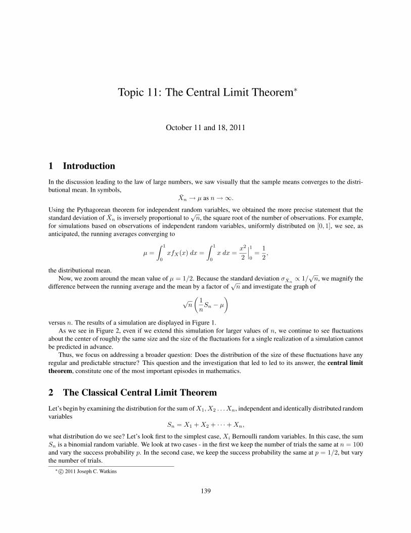
The curves in Figure 3 are looking like bell curves. Their center and spread vary in ways that are predictable. Thebinomial random variable Sn has

mean np and standard deviation√np(1− p).

140


!!!!!!!!!!!!

!

!

!

!

!

!

!

!!

!

!

!

!

!

!

!

!

!!!!!!!!!!!!!!!!!!!!!!!!!!!!!!!!!!!!!!!!!!!!!!!!!!!!!!!!!!!!!!!!!!!!!!!!!!!!!!!!!!!!!!!!!!!!!!!!!!!

!!!!

!

!

!

!

!

!

!

!

!!!

!

!

!

!

!

!

!

!

!!!!!!!!!!!!!!!!!!!!!!!!!!!!!!!!!!!!!!!!!!!!!!!!!!!!!!!!!!!!!!!!!!!!!!!!!!!!!!!!!!!!!!!!!!!!!!!!!!

!!!!

!

!

!

!

!

!

!

!

!!!

!

!

!

!

!

!

!

!

!!!!!!!!!!!!!!!!!!!!!!!!!!!!!!!!!!!!!!!!!!!!!!!!!!!!!!!!!!!!!!!!!!!!!!!!!!!!!!!!!!!!!!!!!!!!!!!!!!!

!!!!

!

!

!

!

!

!

!

!

!!

!

!

!

!

!

!

!

!!!!!!!!!!!!

0 20 40 60 80 100

0.00

0.02

0.04

0.06

0.08

0.10

x

y

!!!!!

!

!

!

!

!

!

!

!

!

!

!

!!!!!!!!!!!!!!!!!!!!!!!!!!!!!!!!!!!!!!!!!!!!!!!!!!!!!!!!!

!!

!

!

!

!

!

!!!

!

!

!

!

!

!!!!!!!!!!!!!!!!!!!!!!!!!!!!!!!!!!!!!!!!!!!!!!!!!!!!!!!!!!!!!!!!!!!

!

!

!

!

!

!!!!

!

!

!

!

!

!

!!!!!!!!!!!!!

0 10 20 30 40 50 60

0.00

0.05

0.10

0.15

x

y

Figure 3: a. Successes in 100 Bernoulli trials with p = 0.2, 0.4, 0.6 and 0.8. b. Successes in Bernoulli trials with p = 1/2 and n = 20, 40 and80.

Thus, if we take the standarized version of these sums of Bernoulli random variables

Zn =Sn − np√np(1− p)

,

then these bell curve graphs would lie on top of each other.For our next example, we look at the density of the sum of standardized exponential random variables. The

exponential density is strongly skewed and so we have have to wait for larger values of n before we see the bell curveemerge. In order to make comparisons, we examine standardized versions of the random variables with mean µ andvariance σ2.

To accomplish this,

• we can either standardize using the sum Sn having mean nµ and standard deviation σ√n, or

• we can standardize using the sample mean Xn having mean µ and standard deviation σ/√n.

This yields two equivalent versions of the z-score.

Zn =Sn − nµσ√n

=Xn − µσ/√n

=√n

σ(Xn − µ). (1)

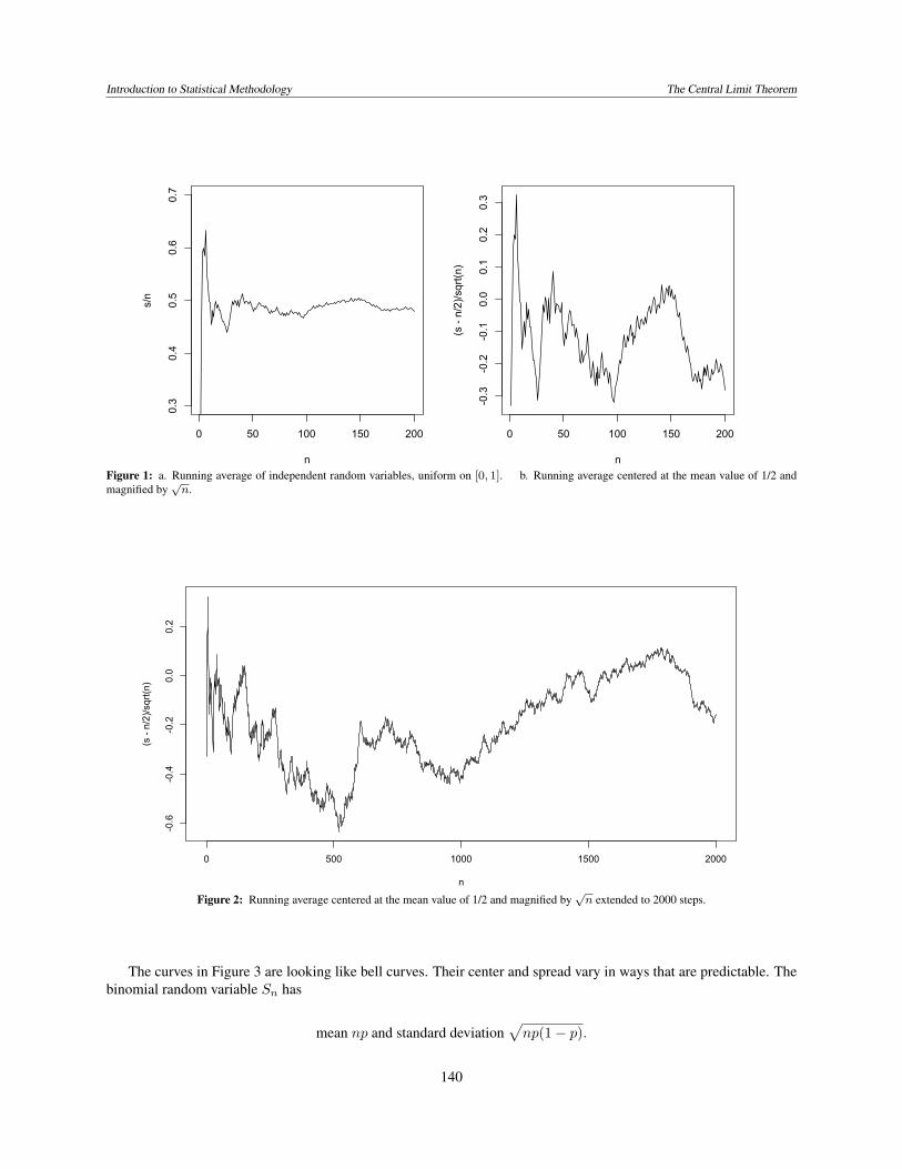
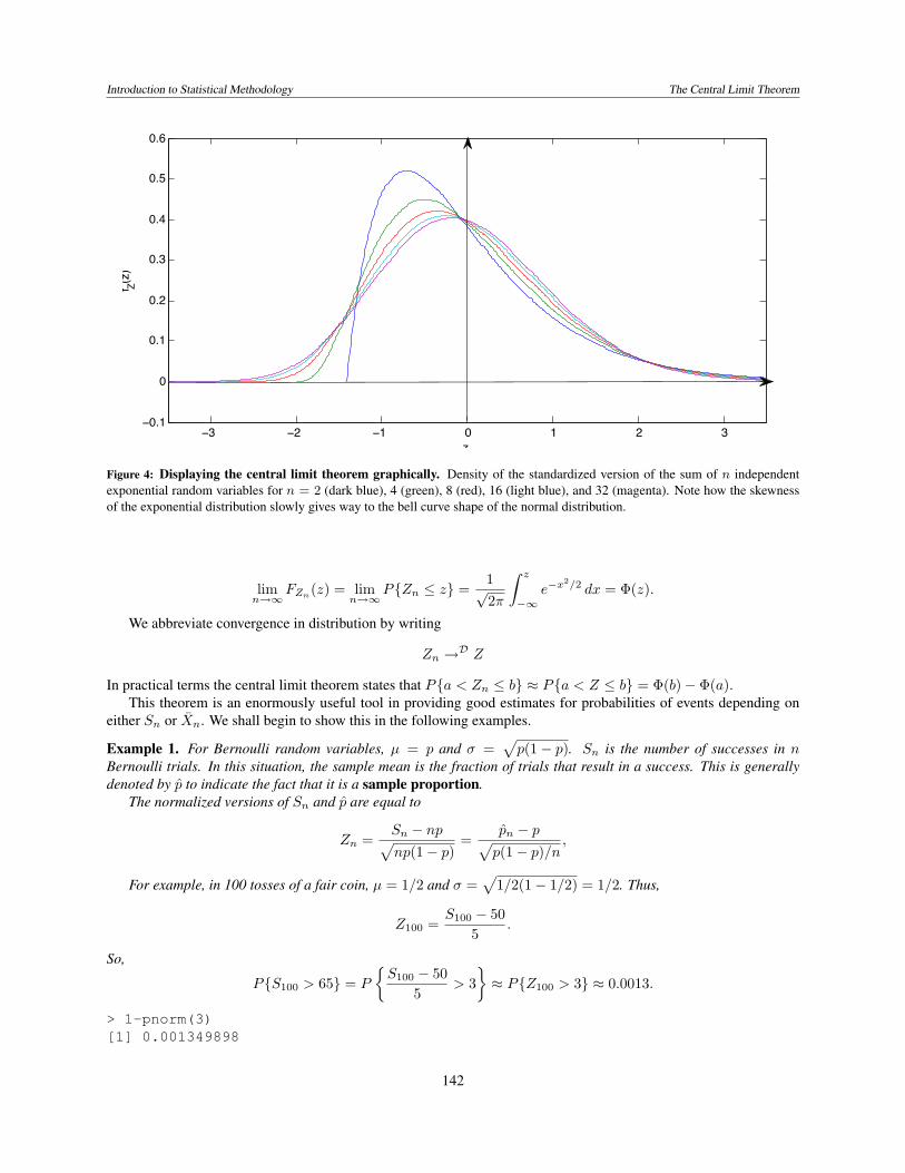
In Figure 4, we see the densities approaching that of the bell curve for a standard normal random variables. Evenfor the case of n = 32, we see a small amount of skewness that is a remnant of the skewness in the exponential density.

The theoretical result behind these numerical explorations is called the classical central limit theorem:

Let {Xi; i ≥ 1} be independent random variables having a common distribution. Let µ be their mean and σ2 betheir variance. Then Zn, the standardized scores defined by equation (1), converges in distribution to Z a standardnormal random variable. More precisely, the distribution function FZn converges to Φ, the distribution function of thestandard normal.

141


!3 !2 !1 0 1 2 3!0.1

0

0.1

0.2

0.3

0.4

0.5

0.6

z

f Z(z)

Figure 4: Displaying the central limit theorem graphically. Density of the standardized version of the sum of n independentexponential random variables for n = 2 (dark blue), 4 (green), 8 (red), 16 (light blue), and 32 (magenta). Note how the skewnessof the exponential distribution slowly gives way to the bell curve shape of the normal distribution.

limn→∞

FZn(z) = limn→∞

P{Zn ≤ z} =1√2π

∫ z

−∞e−x

2/2 dx = Φ(z).

We abbreviate convergence in distribution by writing

Zn →D Z

In practical terms the central limit theorem states that P{a < Zn ≤ b} ≈ P{a < Z ≤ b} = Φ(b)− Φ(a).This theorem is an enormously useful tool in providing good estimates for probabilities of events depending on

either Sn or Xn. We shall begin to show this in the following examples.

Example 1. For Bernoulli random variables, µ = p and σ =√p(1− p). Sn is the number of successes in n

Bernoulli trials. In this situation, the sample mean is the fraction of trials that result in a success. This is generallydenoted by p to indicate the fact that it is a sample proportion.

The normalized versions of Sn and p are equal to

Zn =Sn − np√np(1− p)

=pn − p√p(1− p)/n

,

For example, in 100 tosses of a fair coin, µ = 1/2 and σ =√

1/2(1− 1/2) = 1/2. Thus,

Z100 =S100 − 50

5.

So,

P{S100 > 65} = P

{S100 − 50

5> 3}≈ P{Z100 > 3} ≈ 0.0013.

> 1-pnorm(3)[1] 0.001349898

142


25 26 27 28 29 30 31 32 33 34

0

0.01

0.02

0.03

0.04

0.05

0.06

0.07

0.08

0.09

number of successes

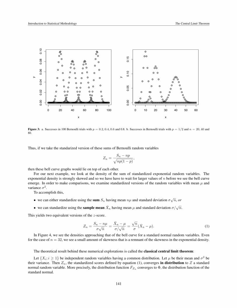
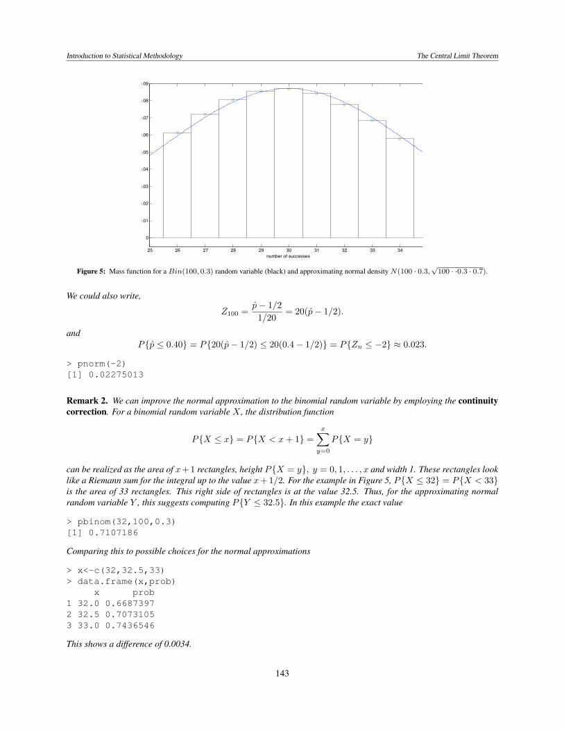
Figure 5: Mass function for a Bin(100, 0.3) random variable (black) and approximating normal density N(100 · 0.3,√

100 · ·0.3 · 0.7).

We could also write,

Z100 =p− 1/2

1/20= 20(p− 1/2).

andP{p ≤ 0.40} = P{20(p− 1/2) ≤ 20(0.4− 1/2)} = P{Zn ≤ −2} ≈ 0.023.

> pnorm(-2)[1] 0.02275013

Remark 2. We can improve the normal approximation to the binomial random variable by employing the continuitycorrection. For a binomial random variable X , the distribution function

P{X ≤ x} = P{X < x+ 1} =x∑y=0

P{X = y}

can be realized as the area of x+ 1 rectangles, height P{X = y}, y = 0, 1, . . . , x and width 1. These rectangles looklike a Riemann sum for the integral up to the value x+ 1/2. For the example in Figure 5, P{X ≤ 32} = P{X < 33}is the area of 33 rectangles. This right side of rectangles is at the value 32.5. Thus, for the approximating normalrandom variable Y , this suggests computing P{Y ≤ 32.5}. In this example the exact value

> pbinom(32,100,0.3)[1] 0.7107186

Comparing this to possible choices for the normal approximations

> x<-c(32,32.5,33)> data.frame(x,prob)

x prob1 32.0 0.66873972 32.5 0.70731053 33.0 0.7436546

This shows a difference of 0.0034.

143


Example 3. Opinion polls are generally designed to be modeled as Bernoulli trials. The number of trials n is set togive a prescribed value m of two times the standard deviation of p. This value of m is an example of a margin oferror. The standard deviation √

p(1− p)/n

takes on its maximum value for p = 1/2. For this case,

m = 2

√12

(1− 1

2

)/n =

1√n

Thus,

n =1m2

We display the results in R for typical values of m.

> m<-seq(0.01,0.05,0.01)> n<-1/mˆ2> data.frame(m,n)

m n1 0.01 10000.0002 0.02 2500.0003 0.03 1111.1114 0.04 625.0005 0.05 400.000

Exercise 4. We have two approximation methods for a large number n of Bernoulli trials - Poisson, which appliesthen p is small and their product λ = np is moderate and normal when the mean number of successes np or the meannumber of failures n(1−p) is sufficiently large. Investigate the approximation of the distribution,X , a Poisson randomvariable, by the distribution of a normal random variable, Y , for the case λ = 16. Use the continuity correction tocompare

P{X ≤ x} to P{Y ≤ x+12}.

Example 5. For exponential random variables µ = 1/λ and σ = 1/λ and therefore

Zn =Sn − n/λ√

n/λ=λSn − n√

n.

Let T64 be the sum of 64 independent with parameter λ = 1. Then, µ = 1 and σ = 1. So,

P{T64 < 60} = P

{T64 − 64

8< −60− 64

8

}= P

{T64 − 64

8< −1

2

}= P{Z64 < −0.5} ≈ 0.309.

Example 6. Video projector light bulbs are known to have a mean lifetime of µ = 100 hours and standard deviationσ = 75. The university uses the projectors for 9000 hours per semester. How likely are 100 light bulbs to be sufficientfor the semester?

Let S100 be the total lifetime of the 100 bulbs. We are asking for the probability that {S100 > 9000}. Note thatthis event is equivalent to

Z100 =S100 − 10000

75 ·√

100>

9000− 1000075 ·√

100= −4

3

and, by the central limit theorem, P{Z100 > 4/3} ≈ 0.909.

Exercise 7. Use the central limit theorem to estimate the number of light bulbs necessary to have a 1% chance ofrunning out of light bulbs before the semester ends.

144


Exercise 8. Simulate 1000 times, x, the sample mean of 100 random variables, uniformly distributed on [0, 1]. Showa histogram for these simulations to see the approximation to a normal distribution. Find the mean and standarddeviations for the simulations and compare them to their distributional values. Use both the simulation and thecentral limit theorem to estimate the 35th percentile of X .

3 Propagation of ErrorPropagation of error or propagation of uncertainty is a strategy to estimate the impact on the standard deviationof the consequences of a nonlinear transformation of a measured quantity whose measurement is subject to someuncertainty.

For any random variable Y with mean µY and standard deviation σY , we will be looking at linear functions aY +bfor Y . Recall that

E[aY + b] = aµY + b, Var(aY + b) = a2Var(Y ).

We will apply this to the linear approximation of g(Y ) about the point µY .

g(Y ) ≈ g(µY ) + g′(µY )(Y − µY ). (2)

If we take expected values, then

Eg(Y ) ≈ E[g(µY ) + g′(µY )(Y − µY )] = g(µY ) + g′(µY )E]Y − µY ] = g(µY ) + 0 = g(µY ).

The variance

Var(g(Y )) ≈ Var(g′(µY )(Y − µY )) = g′(µY )2Var(Y − µY ) = g′(µY )2σ2Y .

Thus, the standard deviationσg(Y ) ≈ |g′(µY )|σY (3)

gives what is known as the propagation of error.If Y is meant to be some measurement of a quantity q with a measurement subject to error, then saying that

q = µY = EY

is stating that Y is an unbiased estimator of q. In other words, Y does not systematically overestimate or under-estimate q. The standard deviation σY gives a sense of the variability in the measurement apparatus. However, ifwe measure Y but want to give not an estimate for q, but an estimate for a function of q, namely g(q), its standarddeviation is approximation by formula (3).

Example 9. Let Y be the measurement of a side of a cube with length `. Then Y 3 is an estimate of the volume of thecube. If the measurement error has standard deviation σY , then, taking g(y) = y3, we see that the standard deviationof the error in the measurement of the volume

σY 3 ≈ 3q2σY .

If we estimate q with Y , thenσY 3 ≈ 3Y 2σY .

To estimate the coefficient volume expansion α3 of a material, we begin with a material of known length `0 attemperature T0 and measure the length `1 at temperature T1. Then, the coefficient of linear expansion

α1 =`1 − `0

`0(T1 − T0).

If the measure length of `1 is Y . We estimate this by

α1 =Y − `0

`0(T1 − T0).

145


Then, if a measurement Y of `1 has variance σ2Y , then

Var(α1) =σ2Y

`20(T1 − T0)2σα1 =

σY`0|T1 − T0|

.

Now, we estimate

α3 =`31 − `30

`30(T1 − T0)by α3 =

Y 3 − `30`30(T1 − T0)

andσα3 ≈ 3Y 2 σY

`30|T1 − T0|.

Exercise 10. In a effort to estimate the angle θ of the sun, the length ` of a shadow from a 10 meter flag pole ismeasured. If σˆ is the standard deviation for the length measurement, use propagation of error to estimate σθ, thestandard deviation in the estimate of the angle.

Often, the function g is a function of several variables. We will show the multivariate propagation of error inthe two dimensional case noting that extension to the higher dimensional case is straightforward. Now, for randomvariables Y1 and Y2 with means µ1 and µ2 and variances σ2

1 and σ22 , the linear approximation about the point (µ1, µ2)

isg(Y1, Y2) ≈ g(µ1, µ2) +

∂g

∂y1(µ1, µ2)(Y1 − µ1) +

∂g

∂y2(µ1, µ2)(Y2 − µ2).

As before,Eg(Y1, Y2) ≈ g(µ1, µ2).

For Y1 and Y2 independent, we also have that the random variables

∂g

∂y1(µ1, µ2)(Y1 − µ1) and

∂g

∂y2(µ1, µ2)(Y2 − µ2)

are independent. Because the variance of the sum of independent random variables is the sum of their variances, wehave the approximation

σ2g(Y1,Y2) = Var(g(Y1, Y2)) ≈ Var(

∂g

∂y1(µ1, µ2)(Y1 − µ1)) + Var(

∂g

∂y2(µ1, µ2)(Y2 − µ2))

=(∂g

∂y1(µ1, µ2)

)2

σ21 +

(∂g

∂y2(µ1, µ2)

)2

σ22 .

and consequently, the standard deviation,

σg(Y1,Y2) ≈

√(∂g

∂y1(µ1, µ2)

)2

σ21 +

(∂g

∂y2(µ1, µ2)

)2

σ22 .

Exercise 11. Repeat the exercise in the case that the height h if the flag poll is also unknown and is measuredindependently of the shadow length with standard deviation σh. Comment on the case in which the two standarddeviations are equal.

Exercise 12. Generalize the formula for the variance to the case of g(Y1, Y2, . . . , Yd) for independent random vari-ables Y1, Y2, . . . , Yd.

Example 13. In the previous example, we now estimate the volume of an `0×w0×h0 rectangular solid with the mea-surements Y1, Y2, and Y3 for, respectively, the length `0, width w0, and height h0 with respective standard deviationsσ`, σw, and σh. Here, we take g(`, w, h) = `wh, then

∂g

∂`(`, w, h) = wh,

∂g

∂w(`, w, h) = `h,

∂g

∂h(`, w, h) = `w

146


and

σg(Y1,Y2,Y3) ≈

√(∂g

∂`(`0, w0, h0)

)2

σ2` +

(∂g

∂w(`0, w0, h0)

)2

σ2w +

(∂g

∂h(`0, w0, h0)

)2

σ2h

=√

(wh)2σ21 + (`h)2σ2

2 + (`w)2σ23 .

4 Delta Method

1 1.5 21

1.5

2

2.5

3

3.5

4

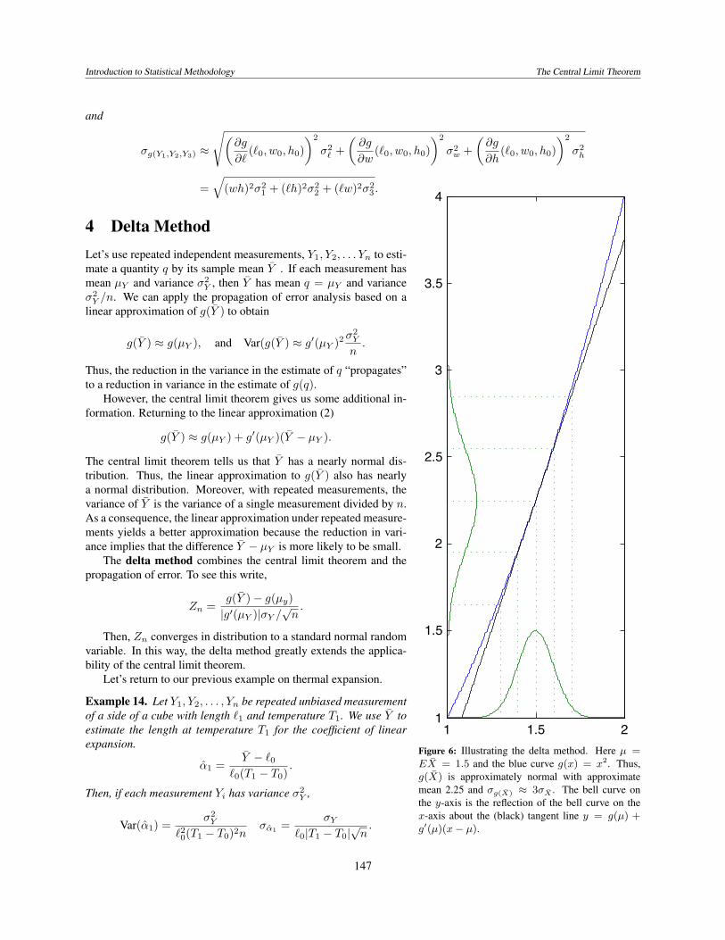
Figure 6: Illustrating the delta method. Here µ =EX = 1.5 and the blue curve g(x) = x2. Thus,g(X) is approximately normal with approximatemean 2.25 and σg(X) ≈ 3σX . The bell curve onthe y-axis is the reflection of the bell curve on thex-axis about the (black) tangent line y = g(µ) +g′(µ)(x− µ).

Let’s use repeated independent measurements, Y1, Y2, . . . Yn to esti-mate a quantity q by its sample mean Y . If each measurement hasmean µY and variance σ2

Y , then Y has mean q = µY and varianceσ2Y /n. We can apply the propagation of error analysis based on a

linear approximation of g(Y ) to obtain

g(Y ) ≈ g(µY ), and Var(g(Y ) ≈ g′(µY )2σ2Y

n.

Thus, the reduction in the variance in the estimate of q “propagates”to a reduction in variance in the estimate of g(q).

However, the central limit theorem gives us some additional in-formation. Returning to the linear approximation (2)

g(Y ) ≈ g(µY ) + g′(µY )(Y − µY ).

The central limit theorem tells us that Y has a nearly normal dis-tribution. Thus, the linear approximation to g(Y ) also has nearlya normal distribution. Moreover, with repeated measurements, thevariance of Y is the variance of a single measurement divided by n.As a consequence, the linear approximation under repeated measure-ments yields a better approximation because the reduction in vari-ance implies that the difference Y − µY is more likely to be small.

The delta method combines the central limit theorem and thepropagation of error. To see this write,

Zn =g(Y )− g(µy)|g′(µY )|σY /

√n.

Then, Zn converges in distribution to a standard normal randomvariable. In this way, the delta method greatly extends the applica-bility of the central limit theorem.

Let’s return to our previous example on thermal expansion.

Example 14. Let Y1, Y2, . . . , Yn be repeated unbiased measurementof a side of a cube with length `1 and temperature T1. We use Y toestimate the length at temperature T1 for the coefficient of linearexpansion.

α1 =Y − `0

`0(T1 − T0).

Then, if each measurement Yi has variance σ2Y ,

Var(α1) =σ2Y

`20(T1 − T0)2nσα1 =

σY`0|T1 − T0|

√n.

147


Now, we estimate the coefficient of volume expansion by

α3 =Y 3 − `30

`30(T1 − T0)

and

σα3 ≈3Y 2σY

`30|T1 − T0|√n.

By the delta method,

Zn =α3 − α3

σα3

has a distribution that can be well approximated by a standard normal random variable.

The next natural step is to take the approach used for the propagation of error in a multidimensional setting and ex-tend the delta method. Focusing on the three dimensional case, we have three independent sequences (Y1,1, . . . , Y1,n1),(Y2,1, . . . , Y2,n2) and (Y3,1, . . . , Y3,n3) of independent random variables. The observations in the i-th sequence havemean µi and variance σ2

i for i = 1, 2 and 3. We shall use Y1, Y2 and Y3 to denote the sample means for the three setsof observations. Then, Yi has

mean µi and variance σ2i

nifor i = 1, 2, 3.

From the propagation of error linear approximation, we obtain

Eg(Y1, Y2, Y3) ≈ g(µ1, µ2, µ3)

and

σ2g(Y1,Y2,Y3) = Var(g(Y1, Y2, Y3)) ≈ ∂g

∂y1(µ1, µ2, µ3)2σ

21

n1+

∂g

∂y2(µ1, µ2, µ3)2σ

22

n2+

∂g

∂y3(µ1, µ2, µ3)2σ

23

n3. (4)

To obtain the normal approximation associated with the delta method, we need to have the additional fact that the sumof independent normal random variables is also a normal random variable. Thus, we have that, for n large,

Zn =g(Y1, Y2, Y3)− g(µ1, µ2, µ3)

σg(Y1,Y2,Y3)

is approximately a standard normal random variable.

Example 15. In avian biology, the fecundity B is defined as the number of female fledglings per female per year. Bis a product of three random variables,

B = F · p ·N,

where µF equals mean number of female fledglings per successful nest, p equals nest survival probability, and µNequals the mean number of nests built per female per year. Let’s collect measurement on n1 nests to count femalefledglings in a successful nest, check n2 nests for survival probability, and follow n3 females to count the number ofsuccessful nests per year. Our experimental design is structured so that measurements are independent. Then, using(4), to B = g(F, p.N) = F · p ·N

σ2B,n =

1n1

(pµNσF )2 +1n2

(µFµFNσp)2 +1n3

(pµFσN )2.

Using the fact that σ2p = p(1 − p) for a Bernoulli random variable, we can write the expression above upon dividing

by µ2B = µ2

F p2µ2N as(

σ2B,n

µB

)2

=1n1

(σFµF

)2

+1n2

(σpp

)2

+1n3

(σNµN

)2

=1n1

(σFµF

)2

+1n2

(1− pp

)+

1n3

(σNµN

)2

.

148


This gives the individual contributions to the variance of B from each of the three data collecting activities. Thevalues of n1, n2, and n3 can be adjusted in the collection of data to minimize the variance of B under a variety ofexperimental designs. In general, the largest choice of the ni should be chosen to reduce the highest of the three ratiosin parentheses..

Estimates for σ2B,n can be found from the field data. Compute sample means

F , p, and N ,

and sample variances2F , p(1− p) and s2

N .

So we estimate the variance in fecundity

s2B,n =

1n1

(pNsF )2 +1n2

(F N)2p(1− p) +1n3

(pF sN )2

Exercise 16. Give the formula for σ2B,n in the case that measurements for F , p, and N are not independent.

This topic leads us naturally to the next topic - a more general discussion of estimation of parameters. We finishthe discussion on the central limit theorem with a summary of some of its applications.

5 Summary of Normal ApproximationsThe z-score of some random quantity is

Z =random quantity−mean

standard deviation.

The central limit theorem and extensions like the delta method tell us when the z-score has an approximatelystandard normal distribution. Thus, using R, we can find good approximations for the probabilities of P{Z < z},pnorm(z) and P{Z > z} using 1-pnorm(z) or P{z1 < Z < z2} using the difference pnorm(z2) -pnorm(z1)

5.1 Sample Sum

-100 -50 0 50 100 150

0.000

0.002

0.004

0.006

0.008

0.010

0.012

x

-100 -50 0 50 100 150

0.000

0.002

0.004

0.006

0.008

0.010

0.012

x

-100 -50 0 50 100 150

0.000

0.002

0.004

0.006

0.008

0.010

0.012

x

-100 -50 0 50 100 150

0.000

0.002

0.004

0.006

0.008

0.010

0.012

x

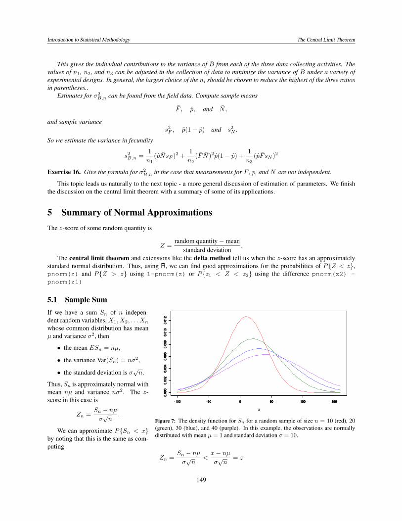
Figure 7: The density function for Sn for a random sample of size n = 10 (red), 20(green), 30 (blue), and 40 (purple). In this example, the observations are normallydistributed with mean µ = 1 and standard deviation σ = 10.

If we have a sum Sn of n indepen-dent random variables, X1, X2, . . . Xn

whose common distribution has meanµ and variance σ2, then

• the mean ESn = nµ,

• the variance Var(Sn) = nσ2,

• the standard deviation is σ√n.

Thus, Sn is approximately normal withmean nµ and variance nσ2. The z-score in this case is


.

We can approximate P{Sn < x}by noting that this is the same as com-puting


<x− nµσ√n

= z

149


and finding P{Zn < z} using the standard normal distribution.

For the special case of Bernoulli trials with success probability p, µ = p and σ =√p(1− p). In this case, normal

approximations often use a continuity correction.

5.2 Sample Mean

-10 -5 0 5 10

0.0

0.1

0.2

0.3

0.4

x

-10 -5 0 5 10

0.0

0.1

0.2

0.3

0.4

x

-10 -5 0 5 10

0.0

0.1

0.2

0.3

0.4

x

-10 -5 0 5 10

0.0

0.1

0.2

0.3

0.4

x

-10 -5 0 5 10

0.0

0.1

0.2

0.3

0.4

x

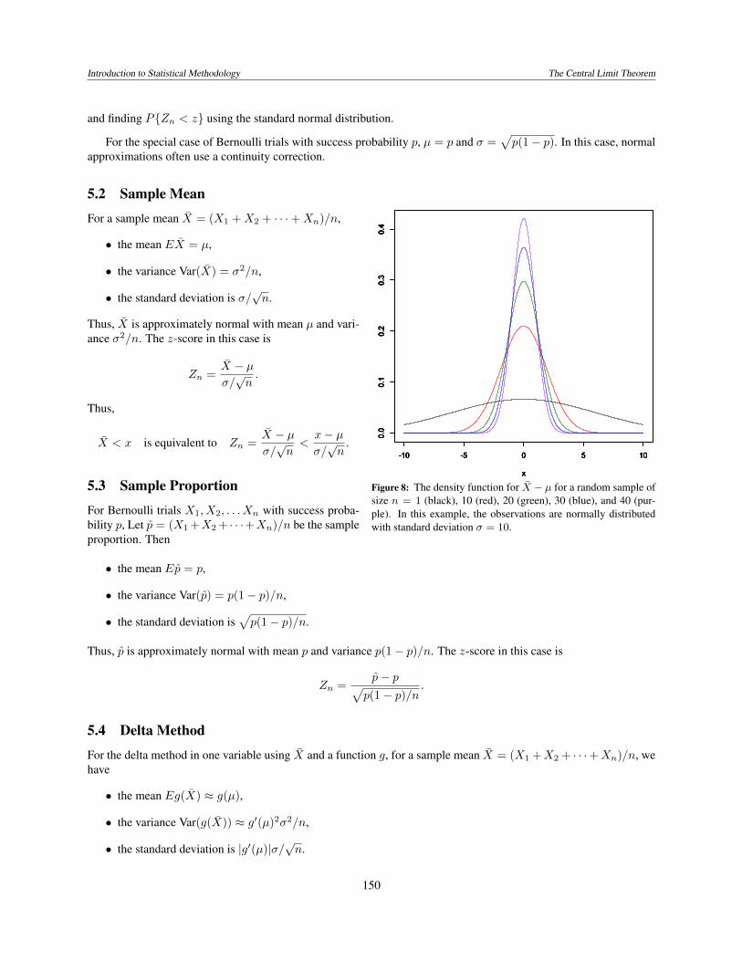
Figure 8: The density function for X − µ for a random sample ofsize n = 1 (black), 10 (red), 20 (green), 30 (blue), and 40 (pur-ple). In this example, the observations are normally distributedwith standard deviation σ = 10.

For a sample mean X = (X1 +X2 + · · ·+Xn)/n,

• the mean EX = µ,

• the variance Var(X) = σ2/n,

• the standard deviation is σ/√n.

Thus, X is approximately normal with mean µ and vari-ance σ2/n. The z-score in this case is

Zn =X − µσ/√n.

Thus,

X < x is equivalent to Zn =X − µσ/√n<x− µσ/√n.

5.3 Sample Proportion

For Bernoulli trials X1, X2, . . . Xn with success proba-bility p, Let p = (X1 +X2 + · · ·+Xn)/n be the sampleproportion. Then

• the mean Ep = p,

• the variance Var(p) = p(1− p)/n,

• the standard deviation is√p(1− p)/n.

Thus, p is approximately normal with mean p and variance p(1− p)/n. The z-score in this case is

Zn =p− p√

p(1− p)/n.

5.4 Delta Method

For the delta method in one variable using X and a function g, for a sample mean X = (X1 +X2 + · · ·+Xn)/n, wehave

• the mean Eg(X) ≈ g(µ),

• the variance Var(g(X)) ≈ g′(µ)2σ2/n,

• the standard deviation is |g′(µ)|σ/√n.

150


Thus, g(X) is approximately normal with mean g(µ) and variance g′(µ)2σ2/n. The z-score is

Zn =g(X)− g(µ)|g′(µ)|σ/

√n.

For the two variable delta method, we now have two independent sequences of independent random variables,X1, X2, . . . Xn1 whose common distribution has mean µ1 and variance σ2

1 and Y1, Y2, . . . Yn2 whose common distri-bution has mean µ2 and variance σ2

2 . For a function g of the sample means, we have that

• the mean Eg(X, Y ) ≈ g(µ1, µ2),

• the variance

Var(g(X, Y )) = σ2g,n ≈

(∂

∂xg(µ1, µ2)

)2σ2

1

n1+(∂

∂yg(µ1, µ2)

)2σ2

2

n2,

• the standard deviation is σg,n.

Thus, g(X, Y ) is approximately normal with mean g(µ1, µ2) and variance σ2g,n. The z-score is

Zn =g(X, Y )− g(µ1, µ2)

σg,n.

The generalization of the delta method to higher dimensional data will add terms to the variance formula.

6 Answers to Selected Exercises

5 10 15 20 25

0.00

0.02

0.04

0.06

0.08

0.10

x

5 10 15 20 25

0.00

0.02

0.04

0.06

0.08

0.10

x

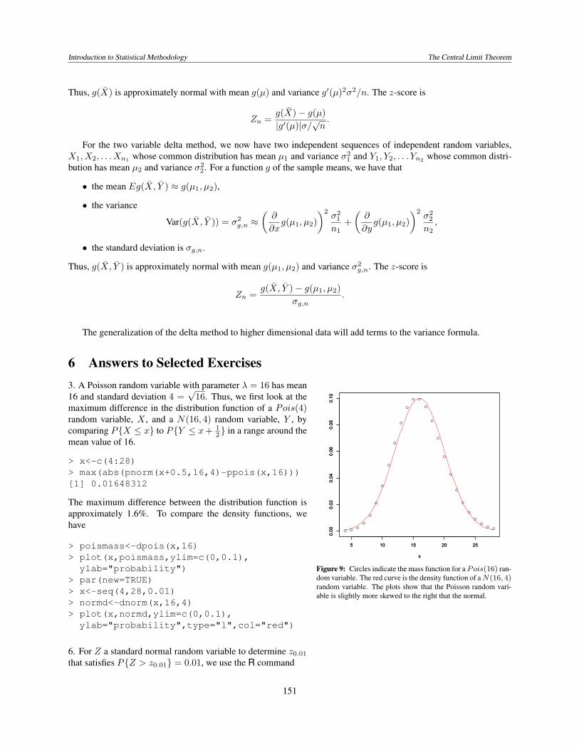
Figure 9: Circles indicate the mass function for a Pois(16) ran-dom variable. The red curve is the density function of a N(16, 4)random variable. The plots show that the Poisson random vari-able is slightly more skewed to the right that the normal.

3. A Poisson random variable with parameter λ = 16 has mean16 and standard deviation 4 =

√16. Thus, we first look at the

maximum difference in the distribution function of a Pois(4)random variable, X , and a N(16, 4) random variable, Y , bycomparing P{X ≤ x} to P{Y ≤ x+ 1

2} in a range around themean value of 16.

> x<-c(4:28)> max(abs(pnorm(x+0.5,16,4)-ppois(x,16)))[1] 0.01648312

The maximum difference between the distribution function isapproximately 1.6%. To compare the density functions, wehave

> poismass<-dpois(x,16)> plot(x,poismass,ylim=c(0,0.1),

ylab="probability")> par(new=TRUE)> x<-seq(4,28,0.01)> normd<-dnorm(x,16,4)> plot(x,normd,ylim=c(0,0.1),

ylab="probability",type="l",col="red")

6. For Z a standard normal random variable to determine z0.01

that satisfies P{Z > z0.01} = 0.01, we use the R command

151


> qnorm(0.99)[1] 2.326348

Thus, we look for the value n that gives a standardized score of z0.01.

2.326348 = z0.01 =100n− 9000

75 ·√n

=4n− 360

3 ·√n

6.979044√n = 4n− 360

48.70705n = 129600− 2880n+ 16n2

0 = 129600− 2928.707n+ 16n2

By the quadratic formula, we solve for n.

n =2928.707 +

√(2928.707)2 − 4 · 16 · 129600

2 · 16= 108.1442

So, take n = 109.Histogram of xbar

xbar

Frequency

0.40 0.45 0.50 0.55 0.60

050

100

150

200

250

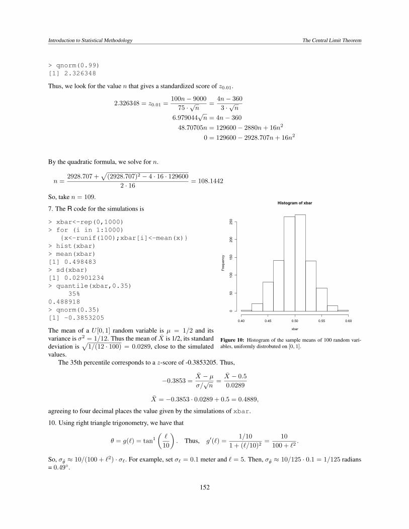
Figure 10: Histogram of the sample means of 100 random vari-ables, uniformly distrobuted on [0, 1].

7. The R code for the simulations is

> xbar<-rep(0,1000)> for (i in 1:1000)

{x<-runif(100);xbar[i]<-mean(x)}> hist(xbar)> mean(xbar)[1] 0.498483> sd(xbar)[1] 0.02901234> quantile(xbar,0.35)

35%0.488918> qnorm(0.35)[1] -0.3853205

The mean of a U [0, 1] random variable is µ = 1/2 and itsvariance is σ2 = 1/12. Thus the mean of X is 1/2, its standarddeviation is

√1/(12 · 100) = 0.0289, close to the simulated

values.The 35th percentile corresponds to a z-score of -0.3853205. Thus,

−0.3853 =X − µσ/√n

=X − 0.50.0289

X = −0.3853 · 0.0289 + 0.5 = 0.4889,

agreeing to four decimal places the value given by the simulations of xbar.

10. Using right triangle trigonometry, we have that

θ = g(`) = tan1

(`

10

). Thus, g′(`) =

1/101 + (`/10)2

=10

100 + `2.

So, σθ ≈ 10/(100 + `2) · σ`. For example, set σ` = 0.1 meter and ` = 5. Then, σθ ≈ 10/125 · 0.1 = 1/125 radians= 0.49◦.

152


11. In this case,

θ = g(`, h) = tan1

(`

h

).

For the partial derivatives, we use the chain rule

∂g

∂`(`, h) =

11 + (`/h)2

(1h

)=

h

h2 + `2∂g

∂h(`, h) =

11 + (`/h)2

(−`h2

)= − `

h2 + `2

Thus,

σθ ≈

√(h

h2 + `2

)2

σ2` +

(`

h2 + `2

)2

σ2h =

1h2 + `2

√h2σ2

` + `2σ2h.

If σh = σ`, let σ denote their common value. Then

σθ ≈1

h2 + `2

√h2σ2 + `2σ2 =

σ√h2 + `2

.

In other words, σθ is inversely proportional to the length of the hypotenuse.

12. Let µi be the mean of the i-th measurement. Then

σg(Y1,Y2,·,Ydt) ≈

√(∂g

∂y1(µ1, . . . , µd)

)2

σ21 +

(∂g

∂y2(µ1, . . . , µd)

)2

σ22 + · · ·+

(∂g

∂yd(µ1, . . . , µd)

)2

σ2d.

14. Recall that for random variables X1, X2, X3 and constants c1, c2, c3,

Var(c0 + c1X1 + c2X2 + c3X3) =3∑i=1

3∑j=3

cicjCov(Xi, Xj) =3∑i=1

3∑j=3

cicjρi,jσiσj .

where ρi,j is the correlation of Xi and Xj . Note that the correlation of a random variable with itself, ρi,i = 1 LetF0, p0, N0 be the actual values of the variables under consideration. Then we have the linear approximation,

g(F , p, N) ≈ g(F0, p0, N0) +∂g

∂F(F0, p0, N0)(F − F0) +

∂g

∂p(F0, p0, N0)(p− p0) +

∂g

∂N(F0, p0, N0)(N −N0).

= g(F0, p0, N0) + p0N0(F − F0) + F0N0(p− p0) + F0p0(N −N0)

Matching this to the covariance formula, we have

c0 = g(F0, p0, N0), c1 = p0N0, c2 = F0N0, c3 = F0p0,

X1 = F , X2 = p, X3 = N .

Thus,

σ2B,n =

1n1

(pNσF )2+1n2

(FNσp)2+1n3

(pFσN )2+2p0F0N20 ρ1,2

σ1σ2√n1n2

+2p20F0N0ρ1,3

σ1σ3√n1n3

+2F 20 p0N0ρ2,3

σ2σ3√n2n3

.

153

Documents

Topic 11: The Central Limit Theoremjwatkins/k-clt.pdf · Topic 11: The Central Limit Theorem October 11 and 18, 2011 1 Introduction In the discussion leading to the law of large numbers,