Embed Size (px)
Citation preview
Topic 4 - Image Mapping - I
DIGITAL IMAGING
Course 3624
Department of Physics and Astronomy
Professor Bob Warwick
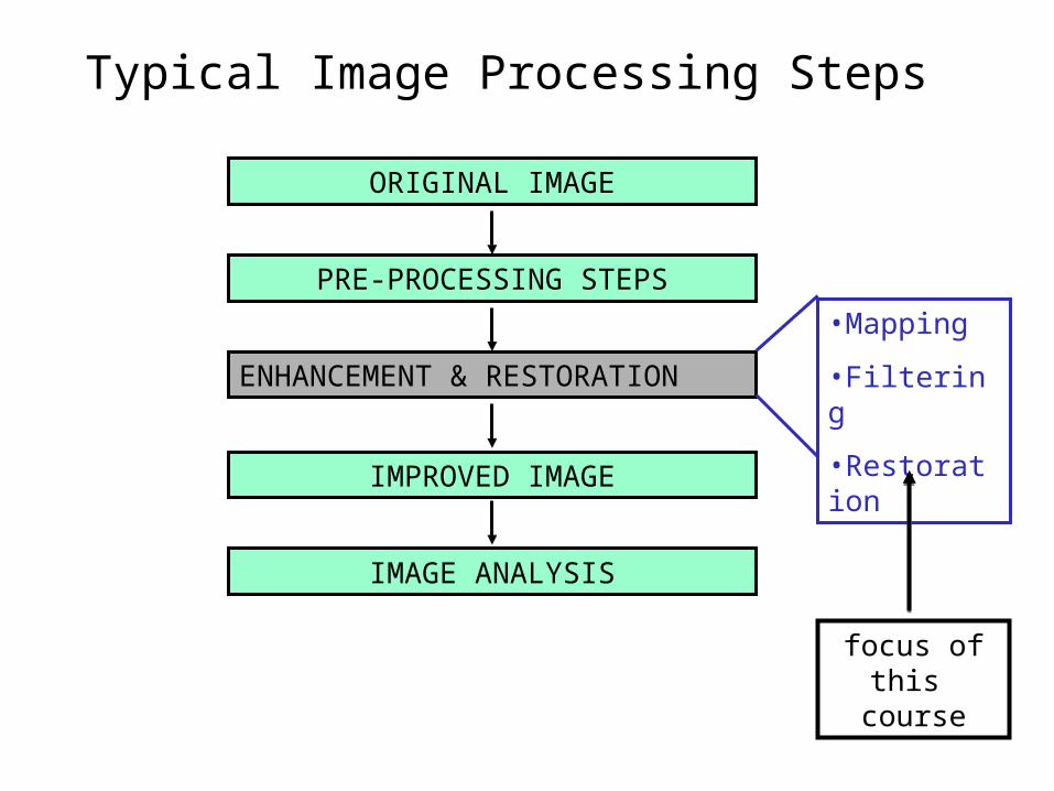
Typical Image Processing Steps
ORIGINAL IMAGE
PRE-PROCESSING STEPS
ENHANCEMENT & RESTORATION
IMPROVED IMAGE
IMAGE ANALYSIS
•Mapping
•Filtering
•Restoration
focus of this course

Image Mapping Processes
Image Mapping encompasses a range of enhancement methods which adjust the way the image data are displayed (ie how the data are "mapped" onto the display device).
4.1 Image Enhancement by Histogram ModificationThe image histogram P(f) is simply the probability distribution of the gray level within the image:
16-level (4-bit) image0 1 2 3 4 5 6 7 8 9 10 11 12 13 14 15
Gray level f
P(f)

Histograms of a Colour Image

The form of the image histogram P(f) provides useful information on the content/quality of the image:
The Form of the Image Histogram
Good contrast Poor contrast Saturated?
Image histogram modification techniques aim to improve the gray level distribution in the displayed image so as to make as much use as possible of the rather limited ability of the eye to discern gray shades.
f f f
P(f
)
P(f
)
P(f
)

Discriminating between Gray Levels - I
I = Intensity of Scene
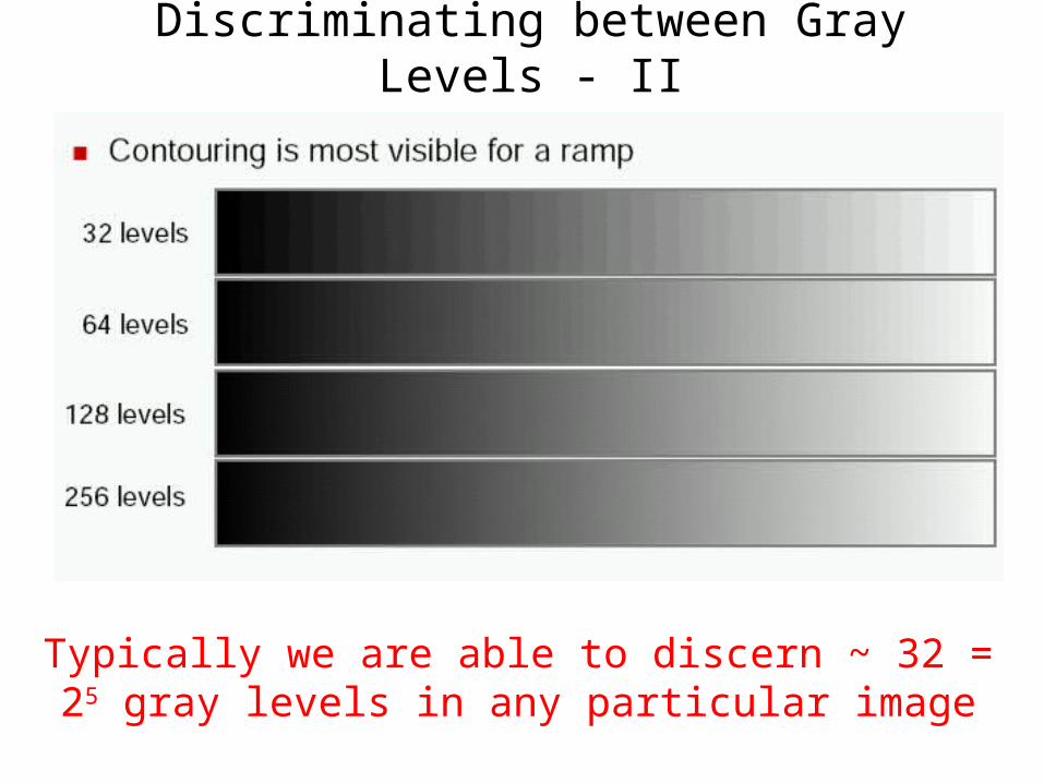
Discriminating between Gray Levels - II
Typically we are able to discern ~ 32 = 25 gray levels in any particular image
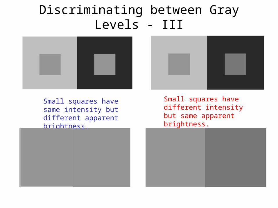
Discriminating between Gray Levels - III
Small squares have same intensity but different apparent brightness.
Small squares have different intensity but same apparent brightness.

Image Enhancement by Histogram Modification
Original Image “New" image
The goal is to find a suitable transformation:
Notes: we assume T(f) is strictly monotonically increasing, i.e., T-1 exists
(Inefficient) Implementation Method:
Once fout = T(fin) has been defined, we compute a new image by fin fout on a pixel-by-pixel basis
15 20 12 25 30 16
15 22 … 25 32 …
… … … … … …
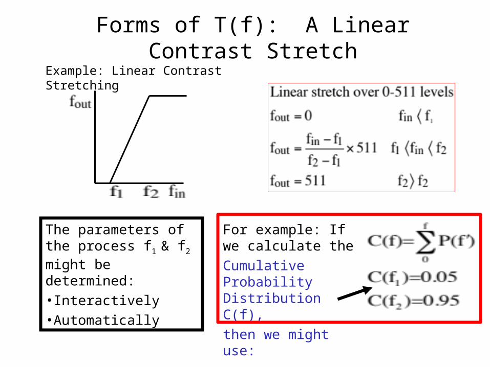
Example: Linear Contrast Stretching
The parameters of the process f1 & f2 might be determined:•Interactively•Automatically
Forms of T(f): A Linear Contrast Stretch
For example: If we calculate the
Cumulative Probability Distribution C(f),
then we might use:
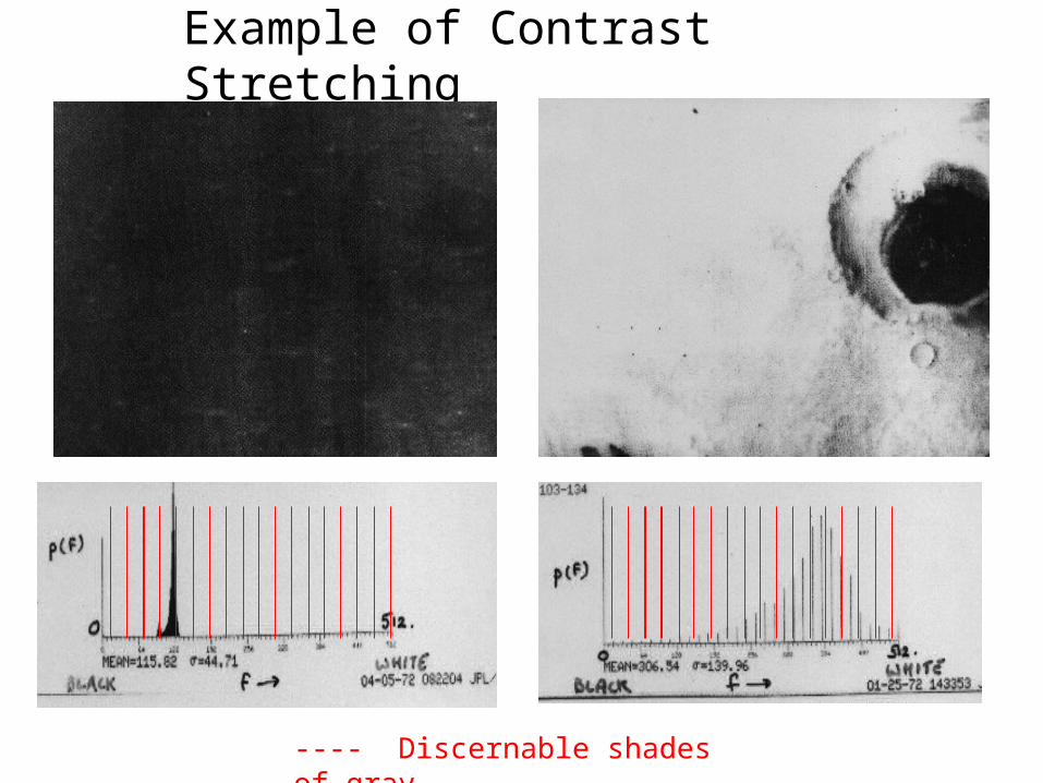
Example of Contrast Stretching
---- Discernable shades of gray

Author: Richard Alan Peters II
Improved Contrast?
0 127 255
012 7
25 5
zero point
sat. point
R+G+B
Author: Richard Alan Peters II
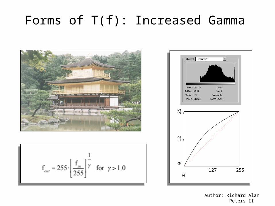
Forms of T(f): Increased Gamma
0 127 255
012 7
25 5
Author: Richard Alan Peters II
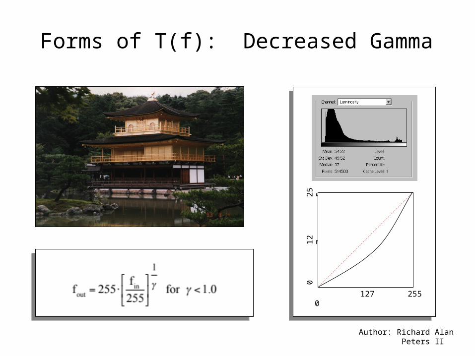
Forms of T(f): Decreased Gamma
0 127 255
012 7
25 5

4.2 Image Enhancement by Histogram Matching
The objective is to set up the displayed image so that its histogram has a specified form.
A special case is HISTOGRAM EQUALISATION where:
P2(fout) = constant i.e. the goal is a uniform distribution. Then:
Notes: •The equations are written in terms of continuous variables
•C1 & C2 are the cumulative distributions of P1 & P2.
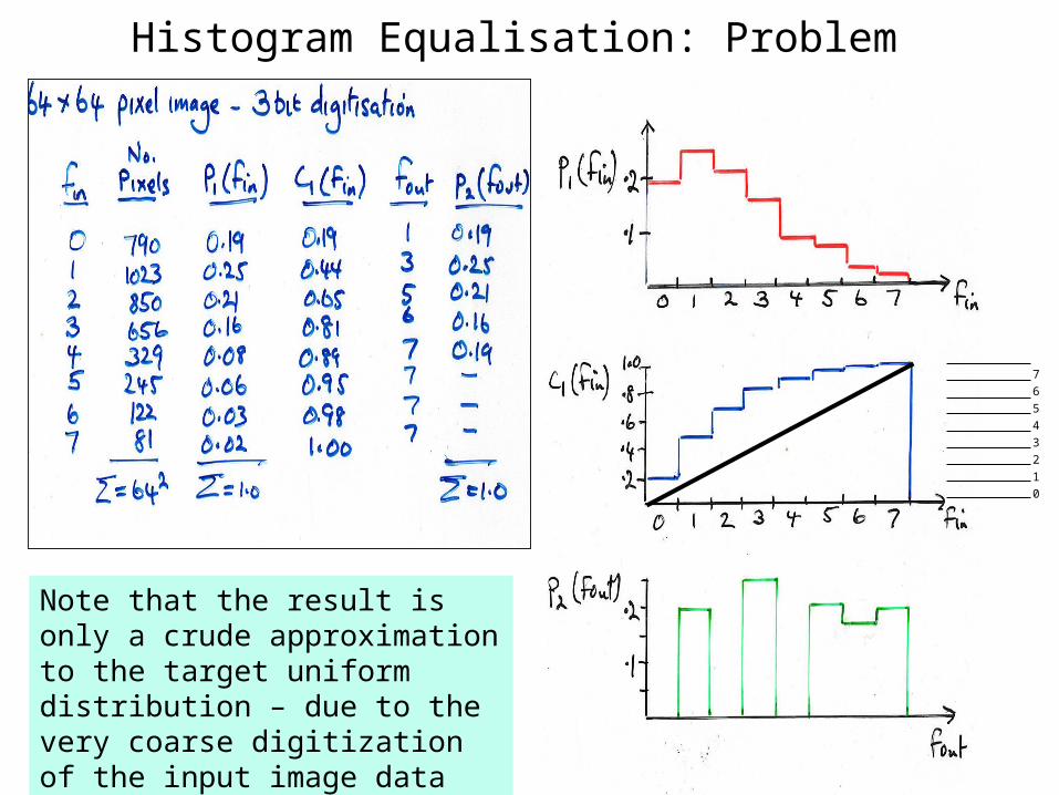
Histogram Equalisation: Problem
7
6
5
4
3
2
1
0
Note that the result is only a crude approximation to the target uniform distribution – due to the very coarse digitization of the input image data
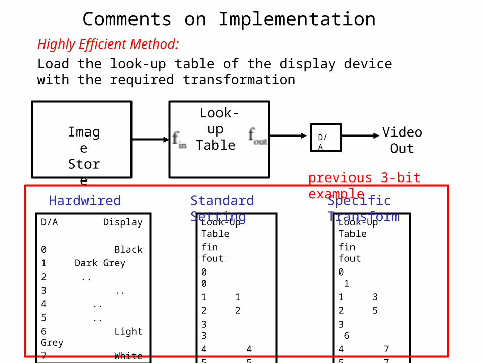
Comments on ImplementationHighly Efficient Method:
Load the look-up table of the display device with the required transformation
Image Store
Look-up Table
D/A Video Out
Look-Up Table
fin fout
0 1
1 3
2 5
3 6
4 7
5 7
6 7
7 7
Specific Transform
D/A Display
0 Black
1 Dark Grey
2 ..
3 ..
4 ..
5 ..
6 Light Grey
7 White
Look-Up Table
fin fout
0 0
1 1
2 2
3 3
4 4
5 5
6 6
7 7
Hardwired Standard Setting
previous 3-bit example
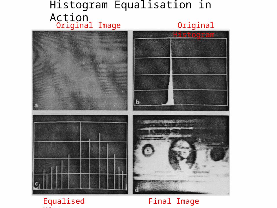
Histogram Equalisation in ActionOriginal Image
Final ImageEqualised Histogram
Original Histogram
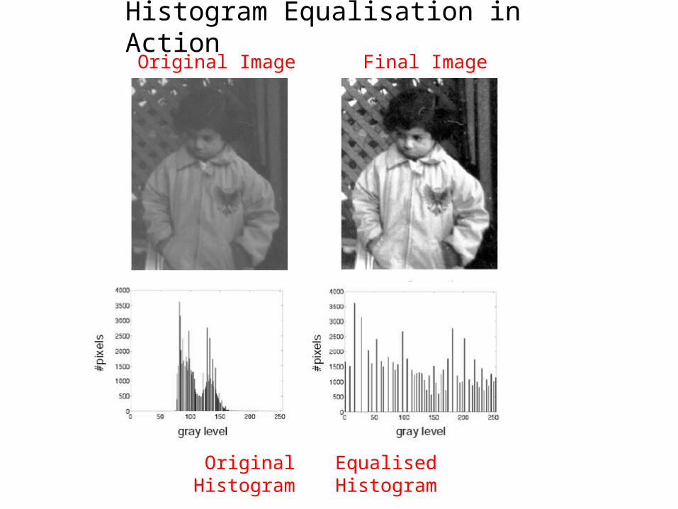
Histogram Equalisation in ActionOriginal Image Final Image
Equalised HistogramOriginal Histogram
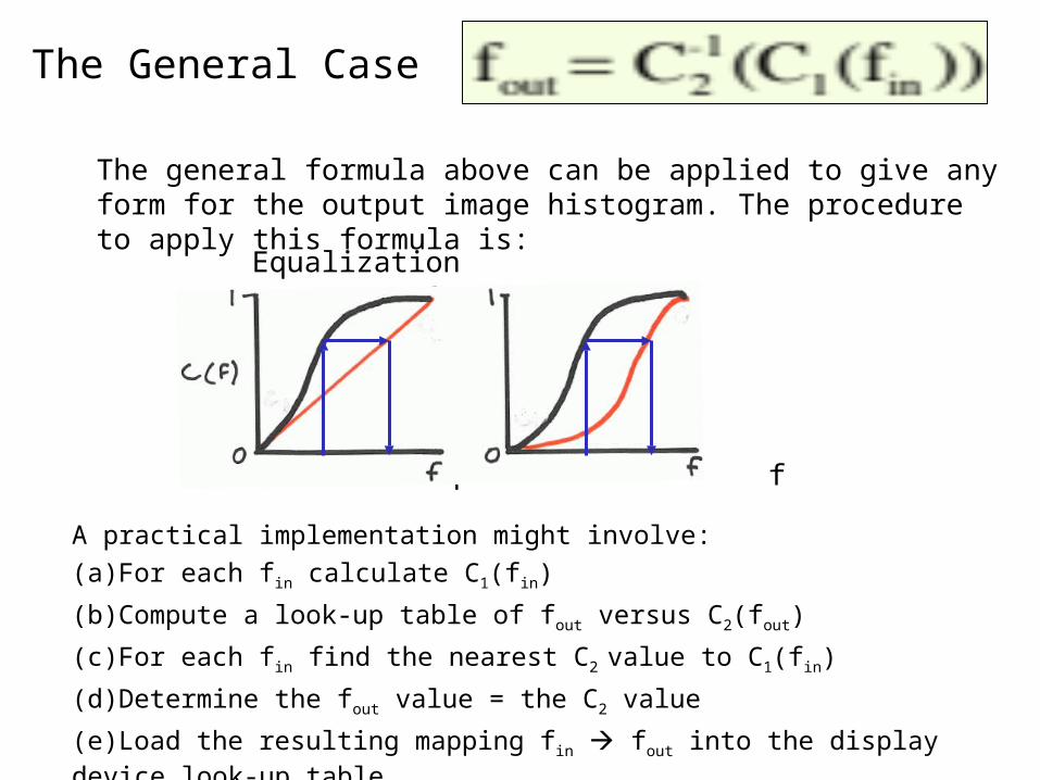
The General Case
The general formula above can be applied to give any form for the output image histogram. The procedure to apply this formula is:
A practical implementation might involve:
(a)For each fin calculate C1(fin)
(b)Compute a look-up table of fout versus C2(fout)
(c)For each fin find the nearest C2 value to C1(fin)
(d)Determine the fout value = the C2 value
(e)Load the resulting mapping fin fout into the display device look-up table
Equalization General
f f
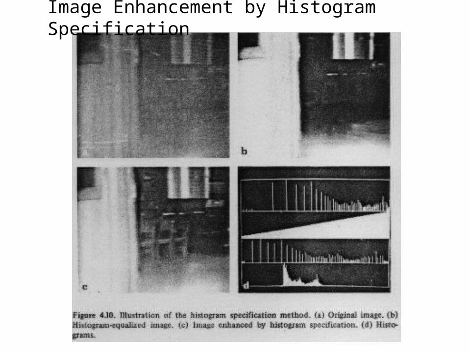
Image Enhancement by Histogram Specification

Author: Richard Alan Peters II
Example: Histogram Specification
Image P(f)
f
Cumulative Distribution
Image C(f)
Author: Richard Alan Peters II
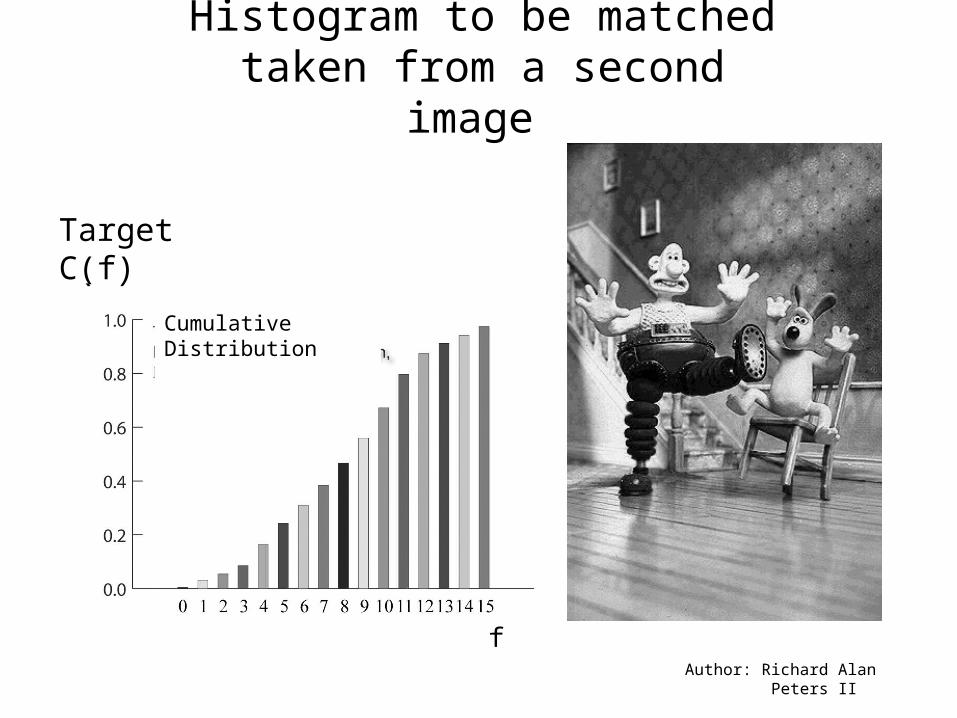
Histogram to be matched taken from a second image
Target P(f)
f
Cumulative Distribution
Target C(f)

Author: Richard Alan Peters II
Image CDFImage CDF Target CDFTarget CDF
Histogram Matching Example
Original RemappedTarget