1

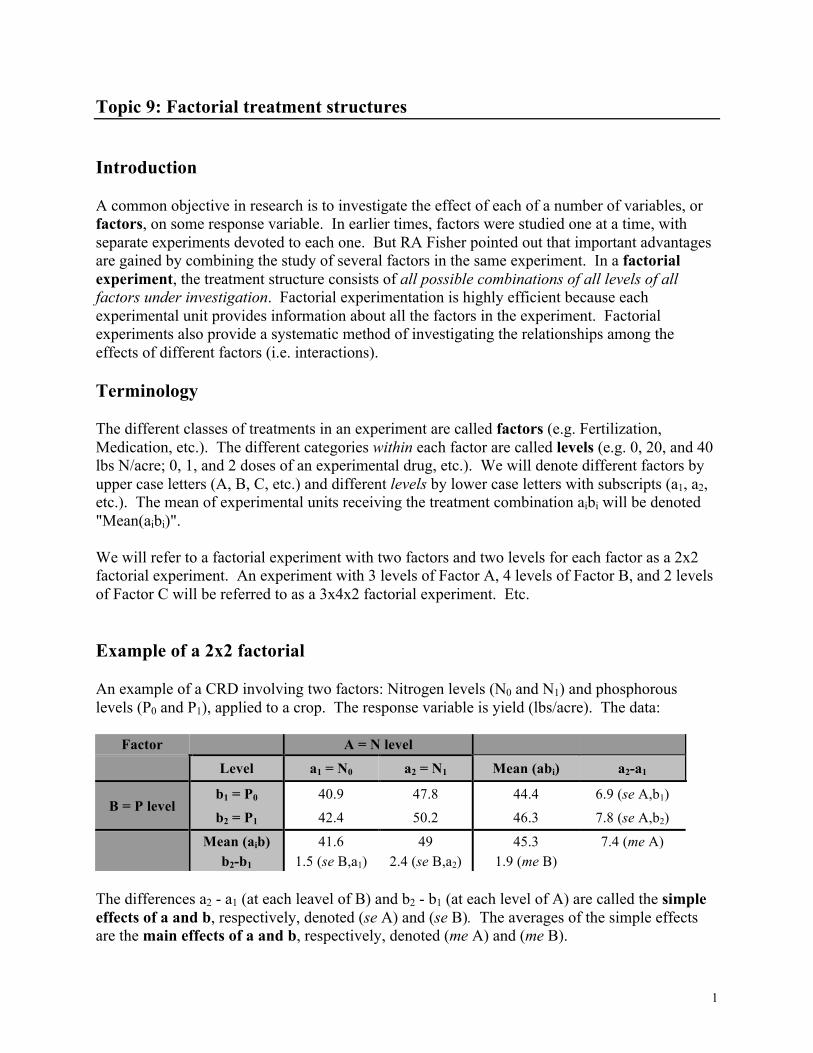
Topic 9: Factorial treatment structures Introduction A common objective in research is to investigate the effect of each of a number of variables, or factors, on some response variable. In earlier times, factors were studied one at a time, with separate experiments devoted to each one. But RA Fisher pointed out that important advantages are gained by combining the study of several factors in the same experiment. In a factorial experiment, the treatment structure consists of all possible combinations of all levels of all factors under investigation. Factorial experimentation is highly efficient because each experimental unit provides information about all the factors in the experiment. Factorial experiments also provide a systematic method of investigating the relationships among the effects of different factors (i.e. interactions). Terminology The different classes of treatments in an experiment are called factors (e.g. Fertilization, Medication, etc.). The different categories within each factor are called levels (e.g. 0, 20, and 40 lbs N/acre; 0, 1, and 2 doses of an experimental drug, etc.). We will denote different factors by upper case letters (A, B, C, etc.) and different levels by lower case letters with subscripts (a1, a2, etc.). The mean of experimental units receiving the treatment combination aibi will be denoted "Mean(aibi)". We will refer to a factorial experiment with two factors and two levels for each factor as a 2x2 factorial experiment. An experiment with 3 levels of Factor A, 4 levels of Factor B, and 2 levels of Factor C will be referred to as a 3x4x2 factorial experiment. Etc. Example of a 2x2 factorial An example of a CRD involving two factors: Nitrogen levels (N0 and N1) and phosphorous levels (P0 and P1), applied to a crop. The response variable is yield (lbs/acre). The data:

Factor A = N level

Level a1 = N0 a2 = N1 Mean (abi) a2-a1

B = P level b1 = P0 40.9 47.8 44.4 6.9 (se A,b1)

b2 = P1 42.4 50.2 46.3 7.8 (se A,b2)

Mean (aib) 41.6 49 45.3 7.4 (me A) b2-b1 1.5 (se B,a1) 2.4 (se B,a2) 1.9 (me B)

The differences a2 - a1 (at each leavel of B) and b2 - b1 (at each level of A) are called the simple effects of a and b, respectively, denoted (se A) and (se B). The averages of the simple effects are the main effects of a and b, respectively, denoted (me A) and (me B).

2

One way of using this data is to consider the effect of N on yield at each P level separately. This information could be useful to a grower who is constrained to use one or the other P level. This is called analyzing the simple effects (se) of N. The simple effects of applying nitrogen are to increase yield by 6.9 lb/acre for P0 and 7.8 lb/acre for P1. It is possible that the effect of N on yield is the same whether or not P is applied. In this case, the two simple effects estimate the same quantity and differ only due to experimental error. One is then justified in averaging the two simple effects to obtain a mean yield response of 7.4 lb/acre. This is called the main effect (me) of N on yield. If the effect of P is independent of N level, then one could do the same thing for this factor and obtain a main effect of P on yield response of 1.9 lb/acre. Interaction If the simple effects of Factor A are the same across all levels of Factor B, the two factors are said to be independent. In such cases, it is appropriate to analyze the main effects of each factor. It may, however, be the case that the effects are not independent. For example, one might expect the application of P to permit a higher expression of the yield potential of the N application. In that case, the effect of N in the presence of P would be much larger than the effect of N in the absence of P. When the effect of one factor depends on the level of another factor, the two factors are said to exhibit an interaction.

An interaction is a measure of the difference in the effect of one factor at the different levels of another factor. Interaction is a common and fundamental scientific idea.

One of the primary objectives of factorial experiments, other than efficiency, is to study the interactions among factors. The sum of squares of an interaction measures the departure of the group means from the values expected on the basis of purely additive effects. In common biological terminology, a large positive deviation of this sort is called synergism. When drugs act synergistically, the result of the interaction of the two drugs may be above and beyond the simple addition of the separate effects of each drug. When the combination of levels of two factors inhibit each other’s effects, we call it interference. Both synergism and interference increase the interaction SS.

3

These differences between the simple effects of two factors, also known as first-order interactions or two-way interactions, can be visualized in the following interaction plots:

a1 a2

se A,b1 b1

b2 Y

se B,a1

a. High me B, no interaction

a1 a2

b1

b2 Y

b. Low me B, no interaction

a1 a2

b1 b2

Y

c. An interaction may be a difference in magnitude of the response

a1 a2

b1

b2

Y

d. It may also be a difference in direction of response

e. Synergism

a1 a2

b1

b2 Y

f. Interference

a1 a2

b1 b2

Y

In interaction plots, perfect additivity (i.e. no interaction) is indicated by perfectly parallel lines. Significant departures from parallel indicate significant interactions.

4

Reasons for carrying out factorial experiments

1. To investigate interactions: If factors are not independent, single factor experiments provide a disorderly, incomplete, and often quite misleading picture of the system. More than this, most of the interesting questions today concern interactions.

2. To establish the dependence or independence of factors of interest: In the initial phases of an

investigation, pilot or exploratory factorial experiments can establish which factors are independent and can therefore be justifiably analyzed in separate experiments.

3. To offer recommendations that must apply over a wide range of conditions: One can

introduce "subsidiary factors" (e.g. soil type) into an experiment to ensure that any recommended results apply across a necessary range of circumstances.

Some disadvantages of factorial experiments 1. The total possible number of treatment level combinations increases rapidly as the number of

factors increases. For example, to investigate 7 factors (3 levels each) in a factorial experiment requires, at minimum, 2187 experimental units.

2. Higher order interactions (three-way, four-way, etc.) are very difficult to interpret. So a large

number of factors complicates the interpretation of results. Differences between nested and factorial experiments (Biometry 322-323) Looking at data table, it is easy to get confused between nested and factorial experiments. Consider a factorial experiment in which leaf discs are grown in 10 different tissue culture media (all possible combinations of 5 different types of sugars and 2 different pH levels). In what way does this differ from a nested design in which each sugar solution is prepared twice, so there are two batches of sugar for each treatment? The following tables represent both designs, using asterisks to represent measurements of the response variable (leaf growth). 2x5 factorial experiment Nested experiment

Sugar Type Sugar Type 1 2 3 4 5 1 2 3 4 5

pH1 * * * * *

Batch 1 * * * * *

* * * * * * * * * *

pH2 * * * * *

Batch 2 * * * * *

* * * * * * * * * *

The data tables look very similar, so what's the difference here? The factorial analysis implies that the two pH classes are common across the entire study (i.e. pH level 1 is a specific pH level that is the same across all sugar treatments). By analogy, if you were to analyze the nested experiment as a two-way factorial ANOVA, it would imply that Batches are common across the

5

entire study. But this is not so. Batch 1 for Treatment 1 has no closer relation to Batch 1 for Treatment 2 than it does to Batch 2 for Treatment 2. "Batch" is an ID, and Batches 1 and 2 are simply arbitrary designations for two randomly prepared sugar solutions for each treatment. Now, if all batches labeled 1 were prepared by the same technician on the same day, while all batches labeled 2 were made by someone else on another day, then “1” and “2” would represent meaningfully common classes across the study. In this case, the experiment could properly be analyzed using a two–way ANOVA with Technicians/Days as blocks (RCBD). While they are both require two-way ANOVAs, RCBD's differ from true factorial experiments in their objective. In this example, we are not interested in the effect of the batches or in the interaction between batches and sugar types. Our main interest is to control for this additional source of variation so that we can better detect the differences among treatments; toward this end, we assume there to be no interactions.

When presented with an experimental description and its accompanying dataset, the critical question to be asked to differentiate factors from experimental units or subsamples is this: Do the classes in question have a consistent meaning across the experiment, or are they simply ID's? Notice that ID (or dummy) classes can be swapped without affecting the analysis (switching the names of "Batch 1" and "Batch 2" within any given Sugar Type has no consequences) whereas factor classes cannot (switching "pH1" and "pH2" within any given Sugar Type will completely muddle the analysis). The two-way factorial analysis (Model I ANOVA) The linear model The linear model for a two-way factorial analysis is

Yijk = µ + τAi + τBj + (τAτB)ij + εijk Here τAi represents the main effect of factor A (i = 1,...,a), τBj represents the main effect of factor B, (j = 1,...,b), (τAτB)ij represents the interaction of factor A level i with factor B level j, and εijk is the error associated with replication k of the factor combination ij (k = 1,..,r). In dot notation:

)()()()( ...................... ijijkjiijjiijk YYYYYYYYYYYY −++−−+−+−+= main effect main effect interaction experimental factor A factor B effect (A*B) error The null hypotheses for a two-factor experiment are τAi = 0, τBj = 0, and (τAτB)ij = 0. The F statistics for each of these hypotheses may be interpreted independently due to the orthogonality of their respective sums of squares.

6

TSS = SSA + SSB + SSAB + SSE The ANOVA In the ANOVA for two-way factorial experiments, the Treatment SS is partitioned into three orthogonal components: a SS for each factor and an interaction SS. This partitioning is valid even when the overall F test among treatments is not significant. Indeed, there are situations where one factor, say B, has no effect on the response variable and hence contributes no more to the SST than one would expect by chance along. In such a circumstance, a significant response to A might well be lost in an overall test of significance. In a factorial experiment, the overall SST is rightly understood to be an intermediate computational quantity rather than an end product (i.e. a numerator for an F test). In a two factor experiment (a x b), there are a total of ab treatment combinations and therefore (ab – 1) treatment degrees of freedom. The main effect of factor A has (a – 1) df and the main effect of factor B has (b – 1) df. The interaction (AxB) has (a – 1)(b – 1) df. With r replications per treatment combination, there are a total of (rab) experimental units in the study and, therefore, (rab – 1) total degrees of freedom. General ANOVA table for a two-way CRD factorial experiment:

Source df SS MS F Factor A a - 1 SSA MSA MSA/MSE Factor B b - 1 SSB MSB MSB/MSE AxB (a - 1)(b - 1) SSAB MSAB MSAB/MSE Error ab(r - 1) SSE MSE Total rab - 1 TSS

The interaction SS is the variation due to the departures of group means from the values expected on the basis of additive combinations of the two factors' main effects. The significance of the interaction F test determines what kind of subsequent analysis is appropriate:

No significant interaction: Subsequent analysis (mean comparisons, contrasts, etc.) are performed on the main effects (i.e. one may compare the means of one factor across all levels of the other factor). Significant interaction: Subsequent analysis (mean comparisons, contrasts, etc.) are performed on the simple effects (i.e. one must compare the means of one factor separately for each level of the other factor).

7

Relationship between factorial experiments and experimental design Experimental designs are characterized by the method of randomization: how were the treatments assigned to the experimental units? In contrast, factorial experiments are characterized by a certain treatment structure, with no requirements on how the treatments are randomly assigned to experimental units. A factorial treatment structure may occur within any experimental design. Example of a 4 x 2 factorial experiment within three different experimental designs: Since Factor A has 4 levels (1, 2, 3, 4) and Factor B has 2 levels (1, 2), there are eight different treatment combinations: (11, 12, 13, 14, 21, 22, 23, 24). CRD with 3 replications

24 23 13 23 24 14 13 23 11 24 12 14 22 13 12 21 21 11 22 12 11 22 21 14 RCBD with 3 blocks

13 12 21 23 11 24 14 22 12 11 24 23 13 22 21 14 24 14 22 21 11 13 23 12 8 x 8 Latin Square

24 11 22 12 13 14 23 21 21 23 13 14 22 12 11 24 12 14 24 11 23 21 22 13 13 22 21 24 11 23 14 12 23 12 11 13 21 22 24 14 14 24 23 22 12 13 21 11 11 21 12 23 14 24 13 22 22 13 14 21 24 11 12 23

8

Example of a 2 x 3 factorial experiment within an RCBD with no significant interactions (ST&D 391) Data: The number of quack-grass shoots per square foot after spraying with maleic hydrazide. Treatments are maleic hydrazide applications rates (R: 0, 4, and 8 lbs/acre) and delay in cultivation after spraying (D: 3 and 10 days).

D R Block 1 Block 2 Block 3 Block 4 Means

3 0 15.7 14.6 16.5 14.7 15.38 4 9.8 14.6 11.9 12.4 12.18 8 7.9 10.3 9.7 9.6 9.38

10 0 18.0 17.4 15.1 14.4 16.23 4 13.6 10.6 11.8 13.3 12.33 8 8.8 8.2 11.3 11.2 9.88

Means 12.30 12.62 12.72 12.60 12.56

The R Code #The ANOVA quack_mod<-lm(Number ~ D + R + D*R + Block, quack_dat) ß WHAT'S MISSING?? anova(quack_mod) Note: If there were only 1 replication per D-R combination (i.e. only 1 block) you could not include the D*R interaction in the model. There would not be enough error df.

The output

Analysis of Variance Table Df Sum Sq Mean Sq F value Pr(>F) D 1 1.500 1.500 0.5713 0.4614 R 2 153.663 76.832 29.2630 6.643e-06 *** Block 3 0.582 0.194 0.0738 0.9731 D:R 2 0.490 0.245 0.0933 0.9114 NS Residuals 15 39.383 2.626

Note that the 15 error df = Block*D (3 df) + Block*R (6 df) + Block*D*R (6 df)

9

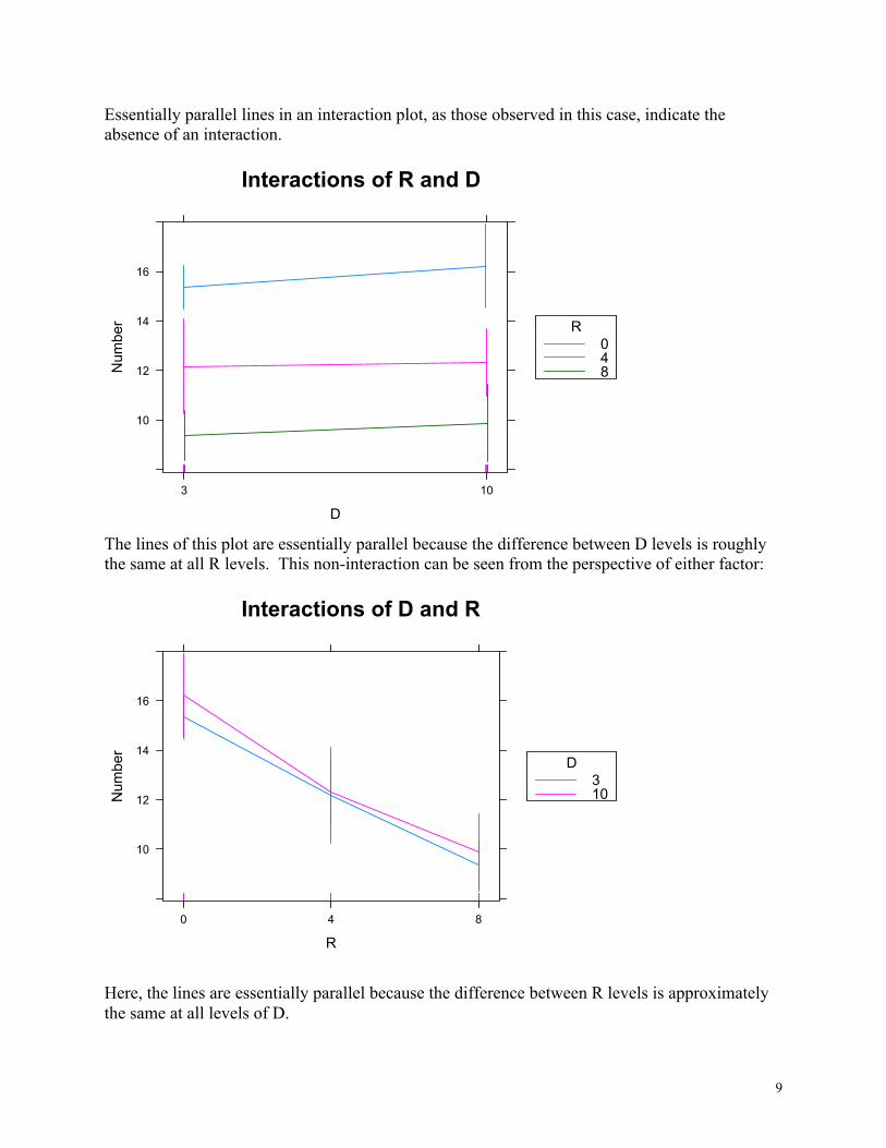
Essentially parallel lines in an interaction plot, as those observed in this case, indicate the absence of an interaction.

The lines of this plot are essentially parallel because the difference between D levels is roughly the same at all R levels. This non-interaction can be seen from the perspective of either factor:

Here, the lines are essentially parallel because the difference between R levels is approximately the same at all levels of D.

Interactions of R and D

D

Number

10

12

14

16

3 10

R048

Interactions of D and R

R

Number

10

12

14

16

0 4 8

D310

10

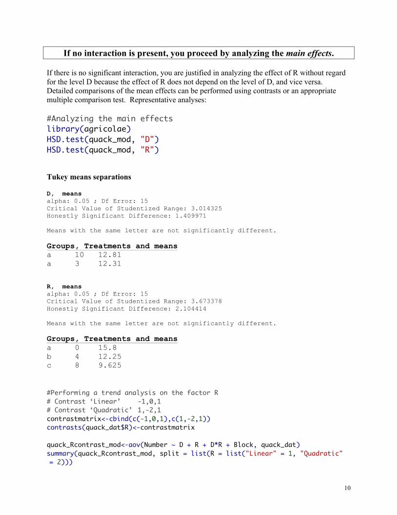
If no interaction is present, you proceed by analyzing the main effects. If there is no significant interaction, you are justified in analyzing the effect of R without regard for the level D because the effect of R does not depend on the level of D, and vice versa. Detailed comparisons of the mean effects can be performed using contrasts or an appropriate multiple comparison test. Representative analyses: #Analyzing the main effects library(agricolae) HSD.test(quack_mod, "D") HSD.test(quack_mod, "R") Tukey means separations D, means alpha: 0.05 ; Df Error: 15 Critical Value of Studentized Range: 3.014325 Honestly Significant Difference: 1.409971 Means with the same letter are not significantly different. Groups, Treatments and means a 10 12.81 a 3 12.31 R, means alpha: 0.05 ; Df Error: 15 Critical Value of Studentized Range: 3.673378 Honestly Significant Difference: 2.104414 Means with the same letter are not significantly different. Groups, Treatments and means a 0 15.8 b 4 12.25 c 8 9.625 #Performing a trend analysis on the factor R # Contrast ‘Linear’ -1,0,1 # Contrast ‘Quadratic’ 1,-2,1 contrastmatrix<-cbind(c(-1,0,1),c(1,-2,1)) contrasts(quack_dat$R)<-contrastmatrix quack_Rcontrast_mod<-aov(Number ~ D + R + D*R + Block, quack_dat) summary(quack_Rcontrast_mod, split = list(R = list("Linear" = 1, "Quadratic" = 2)))

11

Contrasts (trend analysis of R)

Df Sum Sq Mean Sq F value Pr(>F) D 1 1.50 1.50 0.571 0.461 R 2 153.66 76.83 29.263 6.64e-06 *** R: Linear 1 152.52 152.52 58.092 1.56e-06 *** R: Quadratic 1 1.14 1.14 0.435 0.520 Block 3 0.58 0.19 0.074 0.973 D:R 2 0.49 0.25 0.093 0.911 D:R: Linear 1 0.12 0.12 0.047 0.832 D:R: Quadratic 1 0.37 0.37 0.140 0.714 Residuals 15 39.38 2.63 9.7.4.2. Partitioning the Interaction Sum of Squares

It is possible to find significant interaction components within an overall non-significant interaction!

In Topic 4, we discussed how it is possible to find a significant 1 df contrast despite an overall non-significant treatment F test. The concept here is similar. When you divide the Interaction SS by the Interaction df to determine the Interaction MS, you are cutting that SS into equal parts. But it is possible that one component of the interaction (e.g. D * R Linear) is bigger than another (e.g. D * R quadratic), and that that part is significant. Look again at the contrast output above. The trend analysis using orthogonal contrasts partitioned not only the SS for the factor R but also the SS of the interaction D*R. In this way, R makes partitioning the Interaction SS very easy. This can be done another way as well, by "opening up" the factorial treatment structure, as described below: To manually partition the D*R interaction (2 df), you first need to create a variable, say "TRT," whose values are the full set of factorial combinations of D and R levels. The values of TRT for this example would be:

D3 R0 = TRT 1 D10 R0 = TRT 4 D3 R4 = TRT 2 D10 R4 = TRT 5 D3 R8 = TRT 3 D10 R8 = TRT 6

Now we are back in familiar territory. We have "opened up" the factorial treatment structure, redefining it as a simple one-way classification. Now we can simply analyze TRT and use contrasts to partition the interaction, as you've seen before.

12

Modifying the original data table:

D R TRT Block Number3 0 1 1 15.73 0 1 2 14.63 0 1 3 16.5... ... ... ... ...10 8 6 2 8.210 8 6 3 11.310 8 6 4 11.2

Representative code for this approach: #Performing a trend analysis on the factor TRT # TRT Levels: 1 2 3 4 5 6 # Contrast ‘R Linear’ -1 0 1 -1 0 1 # Contrast ‘R Quadratic’ 1 -2 1 1 -2 1 # Contrast ‘D’ 1 1 1 -1 -1 -1 # Contrast ‘R Lin * D’ -1 0 1 1 0 -1 # Contrast ‘R Quad * D’ 1 -2 1 -1 2 -1 contrastmatrix<-cbind(c(-1,0,1,-1,0,1),c(1,-2,1,1,-2,1),

c(1,1,1,-1,-1,-1),c(-1,0,1,1,0,-1),c(1,-2,1,-1,2,-1)) contrasts(quack_dat$TRT)<-contrastmatrix quack_Rcontrast_mod<-aov(Number ~ TRT + Block, quack_dat) summary(quack_Rcontrast_mod, split = list(TRT = list("Lin R" = 1, "Quad R" = 2, "D" = 3, "Lin R * D" = 4, "Quad R * D" = 5)))

The output: Df Sum Sq Mean Sq F value Pr(>F) TRT 5 155.65 31.13 11.857 8.92e-05 *** TRT: Lin R 1 152.52 152.52 58.092 1.56e-06 *** TRT: Quad R 1 1.14 1.14 0.435 0.520 TRT: D 1 1.50 1.50 0.571 0.461 TRT: Lin R * D 1 0.12 0.12 0.047 0.832 TRT: Quad R * D 1 0.37 0.37 0.140 0.714 Block 3 0.58 0.19 0.074 0.973 Residuals 15 39.38 2.63 Here we have successfully partitioned the Treatment SS into its five single-df components, two of which are interaction components. Compare this output to that of the previous factorial analysis:

13

Df Sum Sq Mean Sq F value Pr(>F) D 1 1.50 1.50 0.571 0.461 R 2 153.66 76.83 29.263 6.64e-06 *** R: Linear 1 152.52 152.52 58.092 1.56e-06 *** R: Quadratic 1 1.14 1.14 0.435 0.520 Block 3 0.58 0.19 0.074 0.973 D:R 2 0.49 0.25 0.093 0.911 D:R: Linear 1 0.12 0.12 0.047 0.832 D:R: Quadratic 1 0.37 0.37 0.140 0.714 Residuals 15 39.38 2.63 By "opening up" the factorial treatment structure, we have successfully partitioned the SS of R into its two single-df components and the SS of the D*R interaction into its two single-df components. In this case, no significant interaction components were found "hiding" inside the overall non-significant interaction.

Is it worth partitioning the Interaction SS?

To answer this, divide it by 1 and test for significance. If that is not significant, it is not worth partitioning the Interaction SS

because no significance is found even when all the variation is assigned to one component (1 df) of the interaction.