Topic 9: Optimal Investmentyluo/teaching/6012_2017/lecture9b.pdf · Introducing Adjustment Costs To overcome the –rst problem, we assume that –rms face costs of adjusting their

Topic 9: Optimal Investment

Yulei Luo

Econ HKU

November 29, 2017

Luo, Y. (Econ HKU) Macro Theory November 29, 2017 1 / 22

Demand for Investment

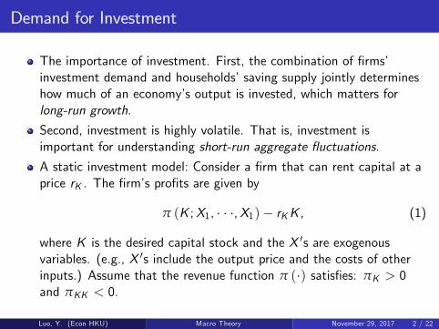
The importance of investment. First, the combination of �rms�investment demand and households�saving supply jointly determineshow much of an economy�s output is invested, which matters forlong-run growth.

Second, investment is highly volatile. That is, investment isimportant for understanding short-run aggregate �uctuations.

A static investment model: Consider a �rm that can rent capital at aprice rK . The �rm�s pro�ts are given by

π (K ;X1, � � �,X1)� rKK , (1)

where K is the desired capital stock and the X 0s are exogenousvariables. (e.g., X 0s include the output price and the costs of otherinputs.) Assume that the revenue function π (�) satis�es: πK > 0and πKK < 0.


Optimal (Desired) Capital Stock

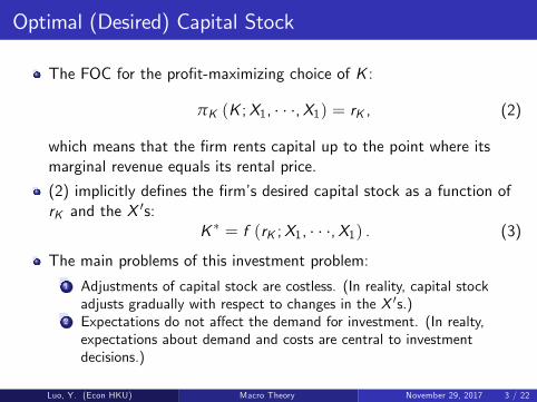
The FOC for the pro�t-maximizing choice of K :

πK (K ;X1, � � �,X1) = rK , (2)

which means that the �rm rents capital up to the point where itsmarginal revenue equals its rental price.

(2) implicitly de�nes the �rm�s desired capital stock as a function ofrK and the X 0s:

K � = f (rK ;X1, � � �,X1) . (3)

The main problems of this investment problem:1 Adjustments of capital stock are costless. (In reality, capital stockadjusts gradually with respect to changes in the X 0s.)

2 Expectations do not a¤ect the demand for investment. (In realty,expectations about demand and costs are central to investmentdecisions.)


Introducing Adjustment Costs

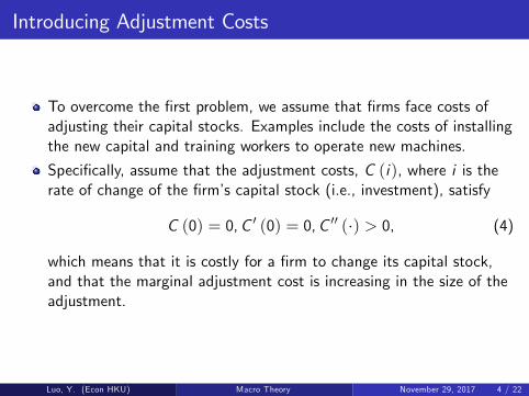
To overcome the �rst problem, we assume that �rms face costs ofadjusting their capital stocks. Examples include the costs of installingthe new capital and training workers to operate new machines.

Speci�cally, assume that the adjustment costs, C (i), where i is therate of change of the �rm�s capital stock (i.e., investment), satisfy

C (0) = 0,C 0 (0) = 0,C 00 (�) > 0, (4)

which means that it is costly for a �rm to change its capital stock,and that the marginal adjustment cost is increasing in the size of theadjustment.


An Investment Model with Adjustment Costs

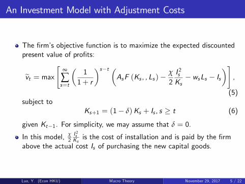
The �rm�s objective function is to maximize the expected discountedpresent value of pro�ts:

evt = max " ∞

∑s=t

�1

1+ r

�s�t �AsF (Ks , , Ls )�

χ

2I 2sKs� wsLs � Is

�#,

(5)subject to

Ks+1 = (1� δ)Ks + Is , s � t (6)

given Kt�1. For simplicity, we may assume that δ = 0.

In this model, χ2I 2sKsis the cost of installation and is paid by the �rm

above the actual cost Is of purchasing the new capital goods.


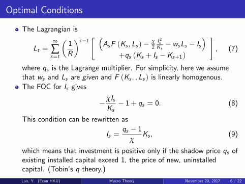
Optimal Conditions

The Lagrangian is

Lt =∞

∑s=t

�1R

�s�t " �AsF (Ks , Ls )� χ2I 2sKs� wsLs � Is

�+qs (Ks + Is �Ks+1)

#, (7)

where qs is the Lagrange multiplier. For simplicity, here we assumethat ws and Ls are given and F (Ks , , Ls ) is linearly homogenous.The FOC for Is gives

�χIsKs� 1+ qs = 0. (8)

This condition can be rewritten as

Is =qs � 1

χKs , (9)

which means that investment is positive only if the shadow price qs ofexisting installed capital exceed 1, the price of new, uninstalledcapital. (Tobin�s q theory.)


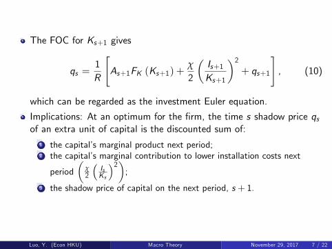
The FOC for Ks+1 gives

qs =1R

"As+1FK (Ks+1) +

χ

2

�Is+1Ks+1

�2+ qs+1

#, (10)

which can be regarded as the investment Euler equation.

Implications: At an optimum for the �rm, the time s shadow price qsof an extra unit of capital is the discounted sum of:

1 the capital�s marginal product next period;2 the capital�s marginal contribution to lower installation costs next

period�

χ2

�IsKs

�2�;

3 the shadow price of capital on the next period, s + 1.


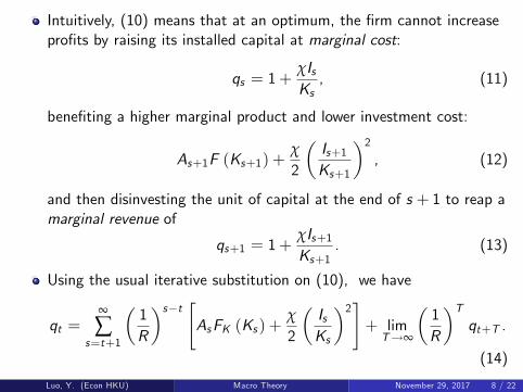
Intuitively, (10) means that at an optimum, the �rm cannot increasepro�ts by raising its installed capital at marginal cost:

qs = 1+χIsKs, (11)

bene�ting a higher marginal product and lower investment cost:

As+1F (Ks+1) +χ

2

�Is+1Ks+1

�2, (12)

and then disinvesting the unit of capital at the end of s + 1 to reap amarginal revenue of

qs+1 = 1+χIs+1Ks+1

. (13)

Using the usual iterative substitution on (10), we have

qt =∞

∑s=t+1

�1R

�s�t "AsFK (Ks ) +

χ

2

�IsKs

�2#+ limT!∞

�1R

�Tqt+T .

(14)


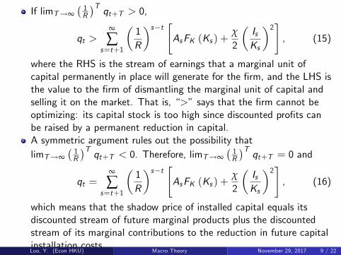
If limT!∞� 1R

�Tqt+T > 0,

qt >∞

∑s=t+1

�1R


χ

2

�IsKs

�2#, (15)

where the RHS is the stream of earnings that a marginal unit ofcapital permanently in place will generate for the �rm, and the LHS isthe value to the �rm of dismantling the marginal unit of capital andselling it on the market. That is, �>�says that the �rm cannot beoptimizing: its capital stock is too high since discounted pro�ts canbe raised by a permanent reduction in capital.A symmetric argument rules out the possibility thatlimT!∞

� 1R

�Tqt+T < 0. Therefore, limT!∞

� 1R

�Tqt+T = 0 and

qt =∞

∑s=t+1

�1R


χ

2

�IsKs

�2#, (16)

which means that the shadow price of installed capital equals itsdiscounted stream of future marginal products plus the discountedstream of its marginal contributions to the reduction in future capitalinstallation costs.Luo, Y. (Econ HKU) Macro Theory November 29, 2017 9 / 22

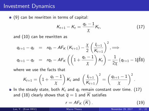
Investment Dynamics

(9) can be rewritten in terms of capital:

Kt+1 �Kt =qt � 1

χKt , (17)

and (10) can be rewritten as

qt+1 � qt = rqt � AFK (Kt+1)�χ

2

�It+1Kt+1

�2,=)

qt+1 � qt = rqt � AFK��

1+qt � 1

χ

�Kt

�� 12χ(qt+1 � 1)2(18)

where we use the facts that

Kt+1 =�1+

qt � 1χ

�Kt and

�It+1Kt+1

�2=

�qt+1 � 1

χ

�2.

In the steady state, both Kt and qt remain constant over time. (17)and (18) clearly shows that q = 1 and K satis�es

r = AFK�K�. (19)


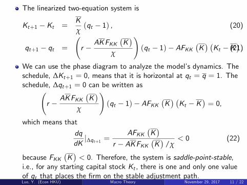
The linearized two-equation system is

Kt+1 �Kt =Kχ(qt � 1) , (20)

qt+1 � qt =

r �

AKFKK�K�

χ

!(qt � 1)� AFKK

�K� �Kt �K

�.(21)

We can use the phase diagram to analyze the model�s dynamics. Theschedule, ∆Kt+1 = 0, means that it is horizontal at qt = q = 1. Theschedule, ∆qt+1 = 0 can be written as

r �AKFKK

�K�

χ

!(qt � 1)� AFKK

�K� �Kt �K

�= 0,

which means that

dqdKj∆qt+1 =

AFKK�K�

r � AKFKK�K�

/χ< 0 (22)

because FKK�K�< 0. Therefore, the system is saddle-point-stable,

i.e., for any starting capital stock Kt , there is one and only one valueof qt that places the �rm on the stable adjustment path.Luo, Y. (Econ HKU) Macro Theory November 29, 2017 11 / 22

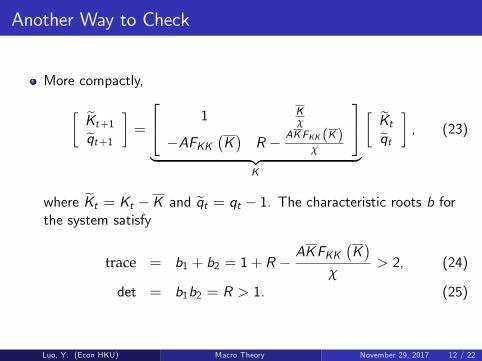
Another Way to Check

More compactly,

� eKt+1eqt+1�=

24 1 Kχ

�AFKK�K�R � AKFKK (K )

χ

35| {z }

K

� eKteqt�, (23)

where eKt = Kt �K and eqt = qt � 1. The characteristic roots b forthe system satisfy

trace = b1 + b2 = 1+ R �AKFKK

�K�

χ> 2, (24)

det = b1b2 = R > 1. (25)


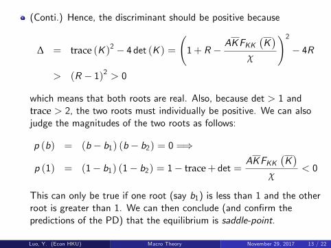
(Conti.) Hence, the discriminant should be positive because

∆ = trace (K )2 � 4 det (K ) = 1+ R �

AKFKK�K�

χ

!2� 4R

> (R � 1)2 > 0

which means that both roots are real. Also, because det > 1 andtrace > 2, the two roots must individually be positive. We can alsojudge the magnitudes of the two roots as follows:

p (b) = (b� b1) (b� b2) = 0 =)

p (1) = (1� b1) (1� b2) = 1� trace+ det =AKFKK

�K�

χ< 0

This can only be true if one root (say b1) is less than 1 and the otherroot is greater than 1. We can then conclude (and con�rm thepredictions of the PD) that the equilibrium is saddle-point.


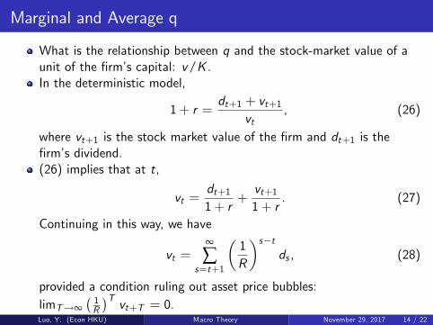
Marginal and Average q

What is the relationship between q and the stock-market value of aunit of the �rm�s capital: v/K .In the deterministic model,

1+ r =dt+1 + vt+1

vt, (26)

where vt+1 is the stock market value of the �rm and dt+1 is the�rm�s dividend.(26) implies that at t,

vt =dt+11+ r

+vt+11+ r

. (27)

Continuing in this way, we have

vt =∞

∑s=t+1

�1R

�s�tds , (28)

provided a condition ruling out asset price bubbles:limT!∞

� 1R

�Tvt+T = 0.


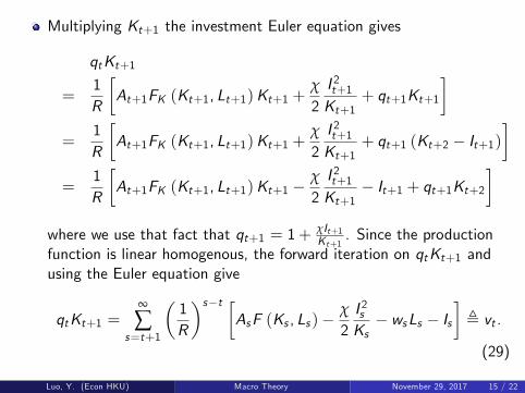
Multiplying Kt+1 the investment Euler equation gives

qtKt+1

=1R

�At+1FK (Kt+1, Lt+1)Kt+1 +

χ

2I 2t+1Kt+1

+ qt+1Kt+1

�=

1R

�At+1FK (Kt+1, Lt+1)Kt+1 +

χ

2I 2t+1Kt+1

+ qt+1 (Kt+2 � It+1)�

=1R

�At+1FK (Kt+1, Lt+1)Kt+1 �

χ

2I 2t+1Kt+1

� It+1 + qt+1Kt+2�

where we use that fact that qt+1 = 1+χIt+1Kt+1

. Since the productionfunction is linear homogenous, the forward iteration on qtKt+1 andusing the Euler equation give

qtKt+1 =∞

∑s=t+1

�1R

�s�t �AsF (Ks , Ls )�

χ

2I 2sKs� wsLs � Is

�, vt .

(29)


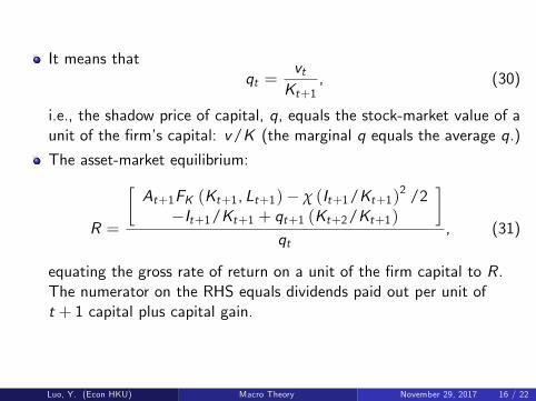
It means thatqt =

vtKt+1

, (30)

i.e., the shadow price of capital, q, equals the stock-market value of aunit of the �rm�s capital: v/K (the marginal q equals the average q.)

The asset-market equilibrium:

R =

�At+1FK (Kt+1, Lt+1)� χ (It+1/Kt+1)

2 /2�It+1/Kt+1 + qt+1 (Kt+2/Kt+1)

�qt

, (31)

equating the gross rate of return on a unit of the �rm capital to R.The numerator on the RHS equals dividends paid out per unit oft + 1 capital plus capital gain.


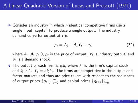
A Linear-Quadratic Version of Lucas and Prescott (1971)

Consider an industry in which n identical competitive �rms use asingle input, capital, to produce a single output. The industrydemand curve for output at t is

pt = A0 � A1Yt + ut , (32)

where A0,A1 > 0, pt is the price of output, Yt is industry output, andut is a demand shock.

The output of each �rm is f0kt where kt is the �rm�s capital stockand f0 > 1. Yt = nf0kt . The �rms are competitive in the output andfactor markets and thus are price takers with respect to the sequencesof output prices fpt+jg∞

j=0 and capital prices fqt+jg∞j=0.


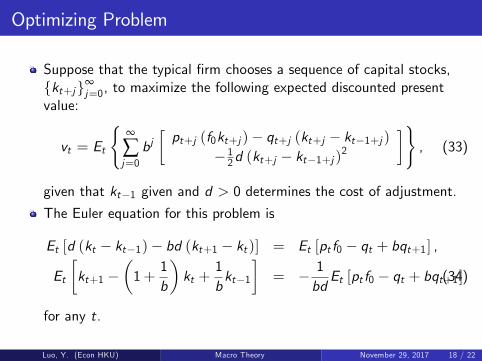
Optimizing Problem

Suppose that the typical �rm chooses a sequence of capital stocks,fkt+jg∞

j=0, to maximize the following expected discounted presentvalue:

vt = Et

(∞

∑j=0bj�pt+j (f0kt+j )� qt+j (kt+j � kt�1+j )

� 12d (kt+j � kt�1+j )

2

�), (33)

given that kt�1 given and d > 0 determines the cost of adjustment.

The Euler equation for this problem is

Et [d (kt � kt�1)� bd (kt+1 � kt )] = Et [pt f0 � qt + bqt+1] ,

Et

�kt+1 �

�1+

1b

�kt +

1bkt�1

�= � 1

bdEt [pt f0 � qt + bqt+1](34)

for any t.


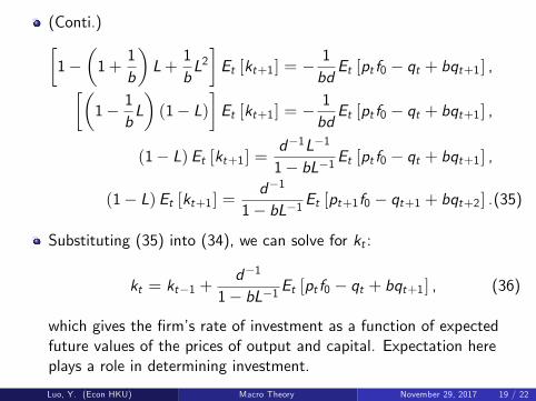
(Conti.)�1�

�1+

1b

�L+

1bL2�Et [kt+1] = �

1bdEt [pt f0 � qt + bqt+1] ,��

1� 1bL�(1� L)

�Et [kt+1] = �

1bdEt [pt f0 � qt + bqt+1] ,

(1� L)Et [kt+1] =d�1L�1

1� bL�1Et [pt f0 � qt + bqt+1] ,

(1� L)Et [kt+1] =d�1

1� bL�1Et [pt+1f0 � qt+1 + bqt+2] .(35)

Substituting (35) into (34), we can solve for kt :

kt = kt�1 +d�1

1� bL�1Et [pt f0 � qt + bqt+1] , (36)

which gives the �rm�s rate of investment as a function of expectedfuture values of the prices of output and capital. Expectation hereplays a role in determining investment.


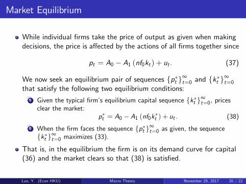
Market Equilibrium

While individual �rms take the price of output as given when makingdecisions, the price is a¤ected by the actions of all �rms together since

pt = A0 � A1 (nf0kt ) + ut . (37)

We now seek an equilibrium pair of sequences fp�t g∞t=0 and fk�t g

∞t=0

that satisfy the following two equilibrium conditions:1 Given the typical �rm�s equilibrium capital sequence fk�t g∞

t=0, pricesclear the market:

p�t = A0 � A1 (nf0k�t ) + ut . (38)

2 When the �rm faces the sequence fp�t g∞t=0 as given, the sequence

fk�t g∞t=0 maximizes (33).

That is, in the equilibrium the �rm is on its demand curve for capital(36) and the market clears so that (38) is satis�ed.


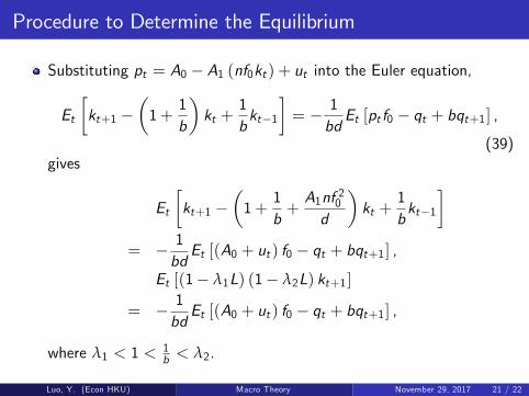
Procedure to Determine the Equilibrium

Substituting pt = A0 � A1 (nf0kt ) + ut into the Euler equation,

Et

�kt+1 �

�1+

1b

�kt +

1bkt�1

�= � 1

bdEt [pt f0 � qt + bqt+1] ,

(39)gives

Et

�kt+1 �

�1+

1b+A1nf 20d

�kt +

1bkt�1

�= � 1

bdEt [(A0 + ut ) f0 � qt + bqt+1] ,

Et [(1� λ1L) (1� λ2L) kt+1]

= � 1bdEt [(A0 + ut ) f0 � qt + bqt+1] ,

where λ1 < 1 < 1b < λ2.


The solution is

Et [k�t+1] = λ1k�t +λ1d�1

1� λ�12 L�1Et [(A0 + ut+1) f0 � qt+1 + bqt+2] ,

(40)for any t, which gives the equilibrium sequence of kt . Substituting(40) into (39), we can solve for the equilibrium k:

k�t = λ1k�t�1 +λ1d�1

1� λ�12 L�1Et [(A0 + ut ) f0 � qt + bqt+1]

= λ1k�t�1 +λ1d

∞

∑i=0

�1

λ2

�iEt [(A0 + ut+i ) f0 � qt+i + bqt+1+i ] .

Substituting the equilibrium k sequence into the market demandschedule gives

p�t = A0 � A1 (nf0k�t ) + ut . (41)

That is, by construction, we have generated sequences, fp�t g∞t=0 and

fk�t g∞t=0 that satisfy the two equilibrium conditions.


Documents

Topic 9: Optimal Investmentyluo/teaching/6012_2017/lecture9b.pdf · Introducing Adjustment Costs To overcome the –rst problem, we assume that –rms face costs of adjusting their