Topic guide 3.2: Processing data using numerical analysis · 1 Unit 3 Analysis of scientic data and information 3.2 Processing data using numerical analysis Data can be analysed for

1

Unit 3: Analysis of scientific data and information

3.2 Processing data using numerical analysis

Data can be analysed for two aspects: patterns and correlation. The former covers maximum/minimum points, gradients and rates of change, whereas the latter is statistical analysis.

On successful completion of this topic you will: • be able to process data using numerical analysis (LO2).

To achieve a Pass in this unit you need to show that you can: • perform numerical analysis on scientific data using an algebraic

method (2.1) • demonstrate numerical analysis using calculus on standard polynomial

equations (2.2) • evaluate absolute errors in scientific data (2.3).

LinkLearners unfamiliar with standard algebraic methods may wish to study M/502/5009 Unit 15: Using Mathematical Tools for Science from Edexcel BTEC Level 2 in Applied Science and A/502/5546 Unit 7: Mathematical Calculations for Science from Edexcel BTEC Level 3 in Applied Science. Alternatively, brief revision notes can be found at the following websites:

http://www.bbc.co.uk/schools/gcsebitesize/maths/algebra/simultaneoushirev1.shtml

http://www.bbc.co.uk/schools/gcsebitesize/maths/algebra/quadequationshirev1.shtml

http://www.bbc.co.uk/schools/gcsebitesize/maths/algebra/graphsrev1.shtml.

http://www.bbc.co.uk/schools/gcsebitesize/maths/algebra/simultaneoushirev1.shtml

http://www.bbc.co.uk/schools/gcsebitesize/maths/algebra/quadequationshirev1.shtml

http://www.bbc.co.uk/schools/gcsebitesize/maths/algebra/graphsrev1.shtml

2


3.2: Processing data using numerical analysis

1 Analysis using algebraic methodsOnce the equation of a trend line has been ascertained, it may need to be manipulated, for example to determine the values of the equation at specific points or to calculate the exact intersection between two trend lines.

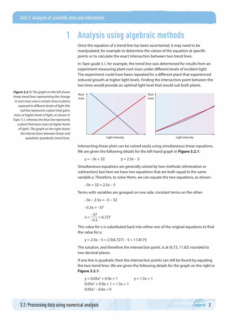
In Topic guide 3.1, for example, the trend line was determined for results from an experiment measuring plant root mass under different levels of incident light. The experiment could have been repeated for a different plant that experienced reduced growth at higher light levels. Finding the intersection point between the two lines would provide an optimal light level that would suit both plants.

Root mass

Light intensity

Root mass

Light intensity

Figure 3.2.1: The graph on the left shows linear trend lines representing the change in root mass over a certain time in plants

exposed to different levels of light (the red line represents a plant that gains

mass at higher levels of light, as shown in Topic 3.1, whereas the blue line represents

a plant that loses mass at higher levels of light). The graph on the right shows

the intersections between linear and quadratic (parabolic) trend lines.

Intersecting linear plots can be solved easily using simultaneous linear equations. We are given the following details for the left-hand graph in Figure 3.2.1:

y = –3x + 32 y = 2.5x – 5

Simultaneous equations are generally solved by two methods (elimination or subtraction) but here we have two equations that are both equal to the same variable y. Therefore, to solve them, we can equate the two equations, as shown:

–3x + 32 = 2.5x – 5

Terms with variables are grouped on one side, constant terms on the other:

–3x – 2.5x = –5 – 32

–5.5x = –37

x = –37–5.5

= 6.727

This value for x is substituted back into either one of the original equations to find the value for y:

y = 2.5x – 5 = 2.5(6.727) – 5 = 11.8175

The solution, and therefore the intersection point, is at (6.73, 11.82) rounded to two decimal places.

If one line is quadratic then the intersection points can still be found by equating the two trend lines. We are given the following details for the graph on the right in Figure 3.2.1:

y = 0.05x2 + 0.9x + 1 y = 1.5x + 10.05x2 + 0.9x + 1 = 1.5x + 10.05x2 – 0.6x = 0

3



This equation can then be factorised to:

x(0.05x – 0.6) = 0

Thus the solutions are:

x = 0 0.05x – 0.6 = 0

x = 0.6

0.05 = 12

Therefore the two trend lines intersect at x = 0 and x = 12.

Take it furtherThe following website provides an interactive presentation on some applications of simultaneous equations and algebraic methods in chemistry: http://mathsforchemistry.info/wordpress/index.php/2010/01/simultaneous-equations-in-chemistry/.

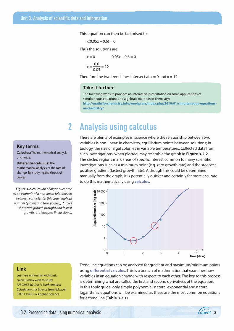
2 Analysis using calculusThere are plenty of examples in science where the relationship between two variables is non-linear: in chemistry, equilibrium points between solutions; in biology, the size of algal colonies in variable temperatures. Collected data from such investigations, when plotted, may resemble the graph in Figure 3.2.2. The circled regions mark areas of specific interest common to many scientific investigations such as a minimum point (e.g. zero growth rate) and the steepest positive gradient (fastest growth rate). Although this could be determined manually from the graph, it is potentially quicker and certainly far more accurate to do this mathematically using calculus.

Time (days)

Alg

al c

ell n

umbe

r (lo

g sc

ale)

542100

1

10

100

1000

10 000

3

Figure 3.2.2: Growth of algae over time as an example of a non-linear relationship

between variables (in this case algal cell number (y-axis) and time (x-axis)). Circles

show zero growth (trough) and fastest growth rate (steepest linear slope).

Trend line equations can be analysed for gradient and maximum/minimum points using differential calculus. This is a branch of mathematics that examines how variables in an equation change with respect to each other. The key to this process is determining what are called the first and second derivatives of the equation. In this topic guide, only simple polynomial, natural exponential and natural logarithmic equations will be examined, as these are the most common equations for a trend line (Table 3.2.1).

Key termsCalculus: The mathematical analysis of change.

Differential calculus: The mathematical analysis of the rate of change, by studying the slopes of curves.

LinkLearners unfamiliar with basic calculus may wish to study A/502/5546 Unit 7: Mathematical Calculations for Science from Edexcel BTEC Level 3 in Applied Science.

4



Standard derivatives (a,b are numbers, x,y are variables)

Equation First derivative Second derivative

Linear y = ax + bdydx

= a

d2ydx2

= 0

Polynomial

y = axb dydx

= abxb–1

d2ydx2

= (ab)(b – 1)xb–2

y = axb + cxdydx

= abxb–1

+ c

Natural exponential y = aebx dydx

= abebx d2y

dx2 = ab2ebx

Natural logarithmic y = alogebx

dydx

=

ax

d2ydx2

= – ax2

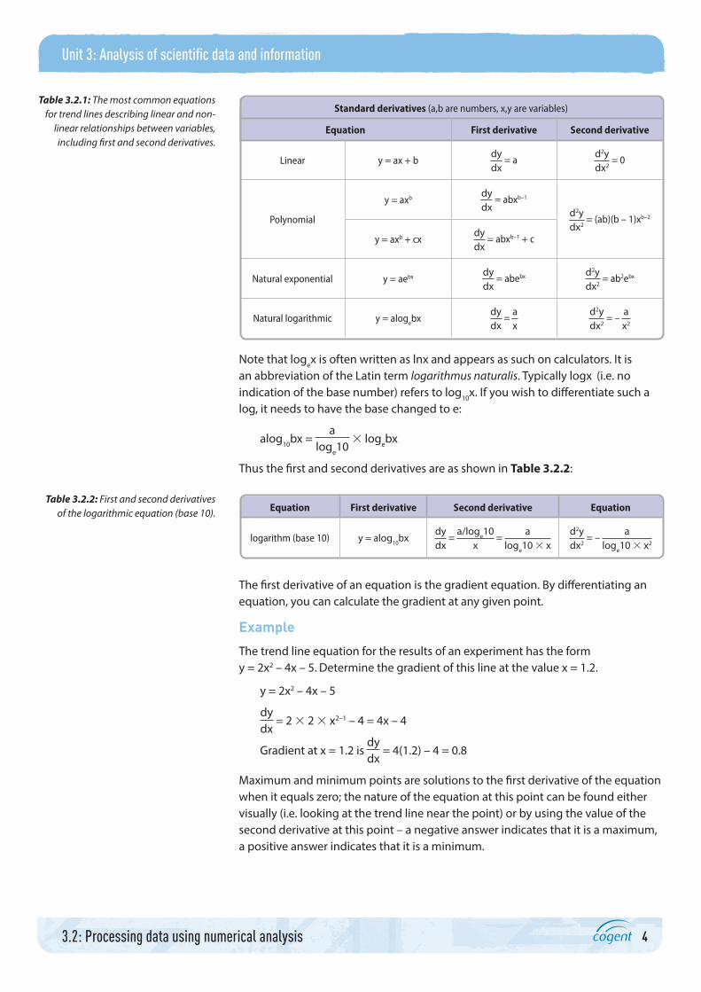
Table 3.2.1: The most common equations for trend lines describing linear and non-

linear relationships between variables, including first and second derivatives.

Note that logex is often written as lnx and appears as such on calculators. It is an abbreviation of the Latin term logarithmus naturalis. Typically logx (i.e. no indication of the base number) refers to log10x. If you wish to differentiate such a log, it needs to have the base changed to e:

alog10bx = a

loge10 3 logebx

Thus the first and second derivatives are as shown in Table 3.2.2:

Equation First derivative Second derivative Equation

logarithm (base 10) y = alog10

bxdydx

=

a/loge10x

=

aloge10 3 x

d2ydx2

= –

aloge10 3 x2

Table 3.2.2: First and second derivatives of the logarithmic equation (base 10).

The first derivative of an equation is the gradient equation. By differentiating an equation, you can calculate the gradient at any given point.

Example

The trend line equation for the results of an experiment has the form y = 2x2 – 4x – 5. Determine the gradient of this line at the value x = 1.2.

y = 2x2 – 4x – 5

dydx

= 2 3 2 3 x2–1 – 4 = 4x – 4

Gradient at x = 1.2 is dydx

= 4(1.2) – 4 = 0.8

Maximum and minimum points are solutions to the first derivative of the equation when it equals zero; the nature of the equation at this point can be found either visually (i.e. looking at the trend line near the point) or by using the value of the second derivative at this point – a negative answer indicates that it is a maximum, a positive answer indicates that it is a minimum.

5



Example

Find the maximum and minimum points in the equation from the previous example.

y = 2x2 – 4x – 5

dydx

= 4x – 4

Set dydx

to zero, dydx

= 0 = 4x – 4

0 = 4x – 4

x = 1 is the solution

d2ydx2 = 4 – this is a positive value, so the equation is a minimum at x = 1

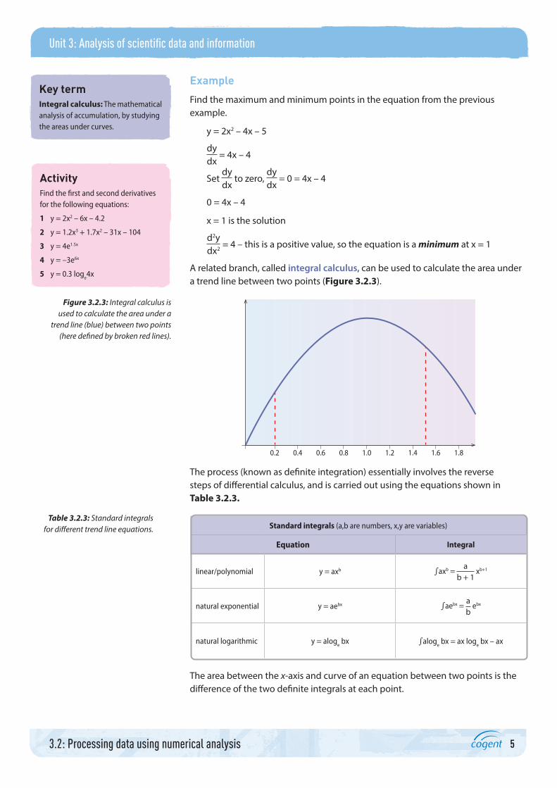
A related branch, called integral calculus, can be used to calculate the area under a trend line between two points (Figure 3.2.3).

0.2 0.4 0.6 0.8 1.0 1.2 1.4 1.81.6

Figure 3.2.3: Integral calculus is used to calculate the area under a

trend line (blue) between two points (here defined by broken red lines).

The process (known as definite integration) essentially involves the reverse steps of differential calculus, and is carried out using the equations shown in Table 3.2.3.

Standard integrals (a,b are numbers, x,y are variables)

Equation Integral

linear/polynomial y = axb eaxb = a

b + 1 xb+1

natural exponential y = aebx eaebx = ab

ebx

natural logarithmic y = aloge bx ealog

e bx = ax log

e bx – ax

Table 3.2.3: Standard integrals for different trend line equations.

The area between the x-axis and curve of an equation between two points is the difference of the two definite integrals at each point.

Key termIntegral calculus: The mathematical analysis of accumulation, by studying the areas under curves.

ActivityFind the first and second derivatives for the following equations:

1 y = 2x2 – 6x – 4.2

2 y = 1.2x3 + 1.7x2 – 31x – 104

3 y = 4e1.5x

4 y = –3e6x

5 y = 0.3 loge4x

6



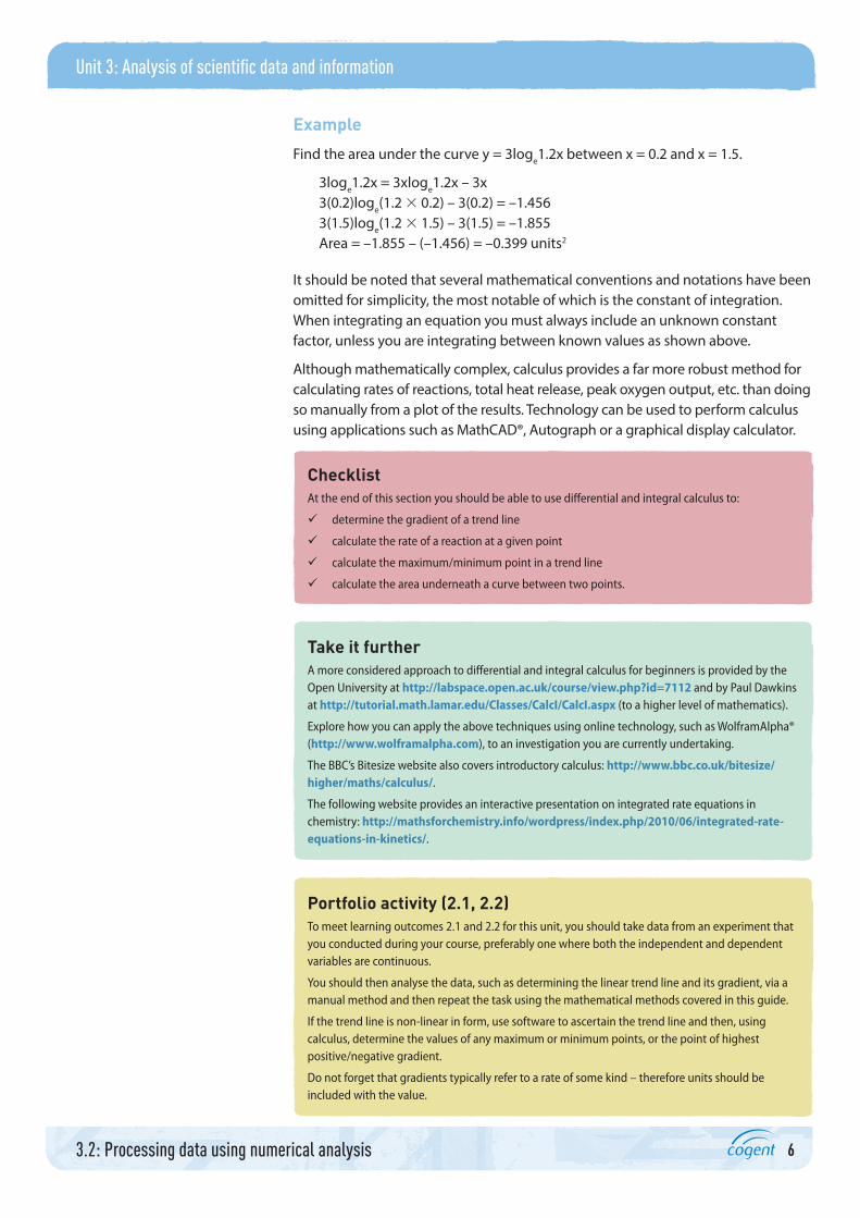
Example

Find the area under the curve y = 3loge1.2x between x = 0.2 and x = 1.5.

3loge1.2x = 3xloge1.2x – 3x3(0.2)loge(1.2 3 0.2) – 3(0.2) = –1.4563(1.5)loge(1.2 3 1.5) – 3(1.5) = –1.855Area = –1.855 – (–1.456) = –0.399 units2

It should be noted that several mathematical conventions and notations have been omitted for simplicity, the most notable of which is the constant of integration. When integrating an equation you must always include an unknown constant factor, unless you are integrating between known values as shown above.

Although mathematically complex, calculus provides a far more robust method for calculating rates of reactions, total heat release, peak oxygen output, etc. than doing so manually from a plot of the results. Technology can be used to perform calculus using applications such as MathCAD®, Autograph or a graphical display calculator.

ChecklistAt the end of this section you should be able to use differential and integral calculus to:

determine the gradient of a trend line

calculate the rate of a reaction at a given point

calculate the maximum/minimum point in a trend line

calculate the area underneath a curve between two points.

Take it furtherA more considered approach to differential and integral calculus for beginners is provided by the Open University at http://labspace.open.ac.uk/course/view.php?id=7112 and by Paul Dawkins at http://tutorial.math.lamar.edu/Classes/CalcI/CalcI.aspx (to a higher level of mathematics).

Explore how you can apply the above techniques using online technology, such as WolframAlpha® (http://www.wolframalpha.com), to an investigation you are currently undertaking.

The BBC’s Bitesize website also covers introductory calculus: http://www.bbc.co.uk/bitesize/ higher/maths/calculus/.

The following website provides an interactive presentation on integrated rate equations in chemistry: http://mathsforchemistry.info/wordpress/index.php/2010/06/integrated-rate-equations-in-kinetics/.

Portfolio activity (2.1, 2.2)To meet learning outcomes 2.1 and 2.2 for this unit, you should take data from an experiment that you conducted during your course, preferably one where both the independent and dependent variables are continuous.

You should then analyse the data, such as determining the linear trend line and its gradient, via a manual method and then repeat the task using the mathematical methods covered in this guide.

If the trend line is non-linear in form, use software to ascertain the trend line and then, using calculus, determine the values of any maximum or minimum points, or the point of highest positive/negative gradient.

Do not forget that gradients typically refer to a rate of some kind – therefore units should be included with the value.

http://www.bbc.co.uk/bitesize/higher/maths/calculus/

http://mathsforchemistry.info/wordpress/index.php/2010/06/integrated-rate-equations-in-kinetics/

7



3 Evaluating absolute errors in dataTypes of errorsWhen collecting data from an experiment or other investigation, the measured values may or may not be the true values that should have been detected. Various factors influence the readings in such a way that there is a quantifiable uncertainty in the stated figures; these values are typically known as errors and they impact on the accuracy and precision of collected data.

• Systematic errors are due to identifiable sources, such as the accuracy of a meter.

• Unsystematic or random errors are caused by unidentifiable or unpredictable sources, such as fluctuations in temperature or differences in physical skills and techniques between experimenters.

• Results that are known to be an error due to carelessness or an accident are classed as mistakes.

• Gross errors are unnoticed mistakes that produce results greatly different from the mean value of the other results.

By testing and calibrating all equipment before (and after) use, as well as evaluating experimental procedures and theoretical models for inconsistencies, systematic errors can be minimised.

Unsystematic errors cannot be directly controlled but their influence can be reduced by training, paying due care and attention, and performing repeated tests and collating more data; they are ultimately accounted for through statistical analysis.

Accuracy and precisionAccuracy

Accuracy is the difference between the measured or calculated size of a quantity and its actual value. It is affected by systematic errors, for example, a poorly calibrated pH meter consistently reading 0.1 above the true value, or a calculation that assumes the speed of light in air is the same as that in a vacuum.

Precision

Precision is the size of the variation in repeated measured or calculated values of a quantity. It is affected by unsystematic errors and mistakes, for example, mechanical vibrations in a room cause a balance to give results that refuse to steady; an experimenter takes visual readings from a burette using an inconsistent method.

Handling errors

Errors in data produced by variables will always have a minimum value (due to the accuracy of the apparatus) that may or may not be measured easily, but they will always ‘remain’ during subsequent calculations and thus need to be handled correctly.

An absolute error is the difference between the exact value and the observed value. A relative error is the absolute error divided by the magnitude of the exact

LinkDifferent types of error and ways of minimising them are discussed in Unit 4: Quality assurance and quality control, Topic guide 4.2.

Key termError: Deviation between an actual value and an observed value or approximation.

8



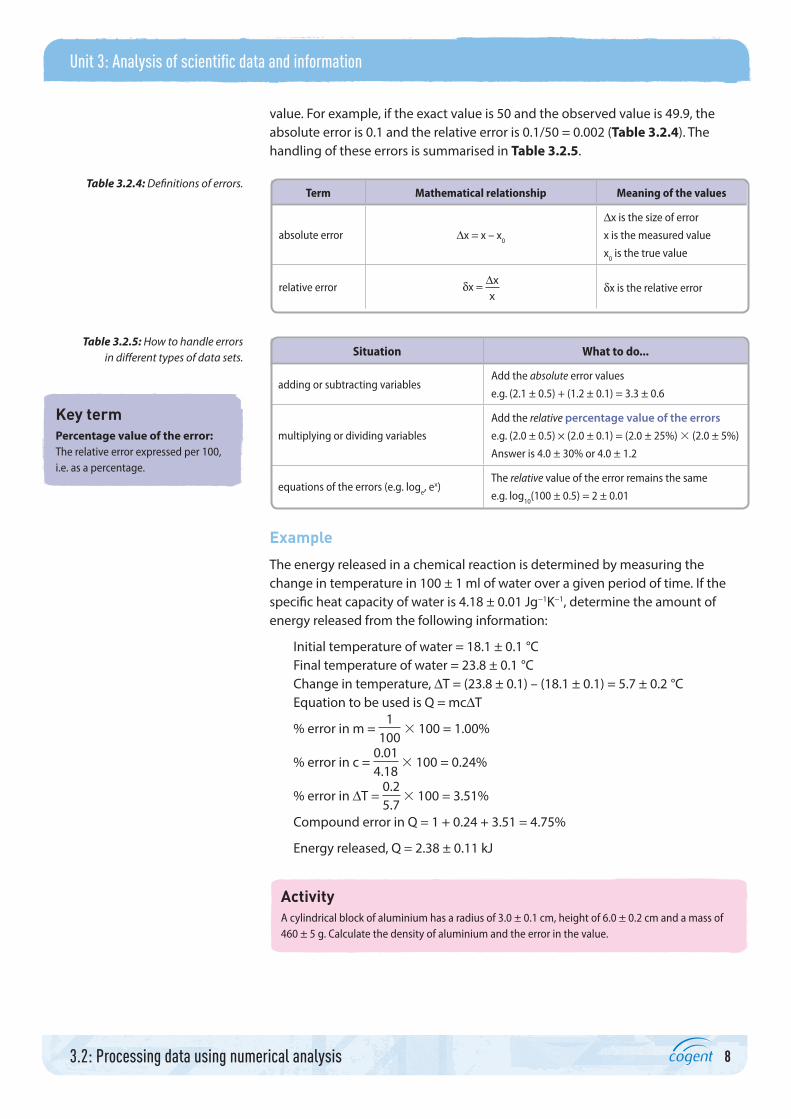
value. For example, if the exact value is 50 and the observed value is 49.9, the absolute error is 0.1 and the relative error is 0.1/50 = 0.002 (Table 3.2.4). The handling of these errors is summarised in Table 3.2.5.

Term Mathematical relationship Meaning of the values

absolute error Dx = x – x0

Dx is the size of error

x is the measured value

x0 is the true value

relative error dx =

Dxx

dx is the relative error

Table 3.2.4: Definitions of errors.

Situation What to do...

adding or subtracting variables Add the absolute error values

e.g. (2.1 ± 0.5) + (1.2 ± 0.1) = 3.3 ± 0.6

multiplying or dividing variables

Add the relative percentage value of the errorse.g. (2.0 ± 0.5) × (2.0 ± 0.1) = (2.0 ± 25%) 3 (2.0 ± 5%)

Answer is 4.0 ± 30% or 4.0 ± 1.2

equations of the errors (e.g. loge, ex)

The relative value of the error remains the same

e.g. log10

(100 ± 0.5) = 2 ± 0.01

Table 3.2.5: How to handle errors in different types of data sets.

Example

The energy released in a chemical reaction is determined by measuring the change in temperature in 100 ± 1 ml of water over a given period of time. If the specific heat capacity of water is 4.18 ± 0.01 Jg−1K−1, determine the amount of energy released from the following information:

Initial temperature of water = 18.1 ± 0.1 °CFinal temperature of water = 23.8 ± 0.1 °CChange in temperature, DT = (23.8 ± 0.1) – (18.1 ± 0.1) = 5.7 ± 0.2 °C Equation to be used is Q = mcDT

% error in m = 1

100 3 100 = 1.00%

% error in c = 0.014.18

3 100 = 0.24%

% error in DT = 0.25.7

3 100 = 3.51%

Compound error in Q = 1 + 0.24 + 3.51 = 4.75%

Energy released, Q = 2.38 ± 0.11 kJ

ActivityA cylindrical block of aluminium has a radius of 3.0 ± 0.1 cm, height of 6.0 ± 0.2 cm and a mass of 460 ± 5 g. Calculate the density of aluminium and the error in the value.

Key termPercentage value of the error: The relative error expressed per 100, i.e. as a percentage.

9



ChecklistAt the end of this topic guide you should be able to evaluate absolute errors in scientific data by:

identifying sources of error

determining procedures to account for and/or quantify errors

calculating relative and compound errors.

Further readingCockett, M. and Doggett, G. (2003) Maths for Chemists, RSC PublishingCroft, A. and Davison, R. (2010) Foundation Maths, Prentice HallOlive, J. (2003) Maths: A Student’s Survival Guide, CUP

AcknowledgementsThe publisher would like to thank the following for their kind permission to reproduce their photographs:

Corbis: Radius Images

Every effort has been made to trace the copyright holders and we apologise in advance for any unintentional omissions. We would be pleased to insert the appropriate acknowledgement in any subsequent edition of this publication.

Documents

Topic guide 3.2: Processing data using numerical analysis · 1 Unit 3 Analysis of scientic data and information 3.2 Processing data using numerical analysis Data can be analysed for