Topics in mathematical modeling and analysis

“volume-vii” — 2012/3/8 — 12:25 — page i — #1

Jindrich Necas Center for Mathematical Modeling

Lecture notes

Volume 7

Topics inmathematicalmodeling and

analysisVolume edited by P. Kaplicky

“volume-vii” — 2012/3/8 — 12:25 — page ii — #2

“volume-vii” — 2012/3/8 — 12:25 — page iii — #3


Lecture notes

Volume 7

Editorial board

Michal Benes

Pavel Drabek

Eduard Feireisl

Miloslav Feistauer

Josef Malek

Jan Maly

Sarka Necasova

Jirı Neustupa

Antonın Novotny

Kumbakonam R. Rajagopal

Hans-Gorg Roos

Tomas Roubıcek

Daniel SevcovicVladimır Sverak

Managing editors

Petr Kaplicky

Vıt Prusa

“volume-vii” — 2012/3/8 — 12:25 — page iv — #4

“volume-vii” — 2012/3/8 — 12:25 — page v — #5

Jindrich Necas Center for Mathematical ModelingLecture notes

Topics in mathematical modelingand analysis

Cherif AmroucheLaboratoire de Mathematiques et deleurs ApplicationsBatiment IPRA - Universite de Pau etdes Pays de l’AdourAvenue de l’Universite - BP 115564013 PAU CEDEXFrance

David E. EdmundsDepartment of MathematicsUniversity of SussexBrighton BN1 9QHUnited Kingdom

Enrique

Fernandez-CaraDepartamento Ecuaciones Diferencialesy Analisis NumericoUniversidad de SevillaTarfia s/n, 41012 SevillaSpain

Anna Hundertmark-

ZauskovaInstitute of MathematicsJohannes Gutenberg UniversityStaudingerweg 9, 55099 MainzGermany

Ron KermanDepartment of MathematicsBrock University500 Glenridge AvenueSt. Catharines, ONL2S 3A1, Canada

Maria

Lukacova-MedvidovaInstitute of MathematicsJohannes Gutenberg UniversityStaudingerweg 9, 55099 MainzGermany

Gabriela RusnakovaInstitute of MathematicsPavol Jozef Safarik UniversityJesenna 5, 040 01 KosiceSlovakia

Arghir ZarnescuMathematical InstituteUniversity of Oxford24-29 St. Giles’Oxford OX1 3LBUnited Kingdom

Volume edited by P. Kaplicky

“volume-vii” — 2012/3/8 — 12:25 — page vi — #6

2000 Mathematics Subject Classification. 35-06

Key words and phrases. weighted Sobolev spaces, Orlicz spaces, generalizedtrigonometric functions, optimal control, fluid-structure interaction, liquid crystals

Abstract. The text provides a record of lectures given by the visitors of the Jindrich NecasCenter for Mathematical Modeling during academic year 2010/2011.

All rights reserved, no part of this publication may be reproduced or transmitted in any formor by any means, electronic, mechanical, photocopying or otherwise, without the prior writtenpermission of the publisher.

c© Jindrich Necas Center for Mathematical Modeling, 2012c© MATFYZPRESS Publishing House of the Faculty of Mathematics and Physics

Charles University in Prague, 2012

ISBN 978-80-7378-196-5

“volume-vii” — 2012/3/8 — 12:25 — page vii — #7

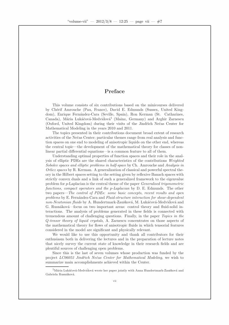
Preface

This volume consists of six contributions based on the minicourses deliveredby Cherif Amrouche (Pau, France), David E. Edmunds (Sussex, United King-dom), Enrique Fernandez-Cara (Seville, Spain), Ron Kerman (St. Catharines,Canada), Maria Lukacova-Medvidova1 (Mainz, Germany) and Arghir Zarnescu(Oxford, United Kingdom) during their visits of the Jindrich Necas Center forMathematical Modeling in the years 2010 and 2011.

The topics presented in their contributions document broad extent of researchactivities of the Necas Center; particular themes range from real analysis and func-tion spaces on one end to modeling of anisotropic liquids on the other end, whereasthe central topic—the development of the mathematical theory for classes of non-linear partial differential equations—is a common feature to all of them.

Understanding optimal properties of function spaces and their role in the anal-ysis of elliptic PDEs are the shared characteristics of the contributions WeightedSobolev spaces and elliptic problems in half-space by Ch. Amrouche and Analysis inOrlicz spaces by R. Kerman. A generalization of classical and powerful spectral the-ory in the Hilbert spaces setting to the setting given by reflexive Banach spaces withstrictly convex duals and a link of such a generalized framework to the eigenvalueproblem for p-Laplacian is the central theme of the paper Generalised trigonometricfunctions, compact operators and the p-Laplacian by D. E. Edmunds. The othertwo papers—The control of PDEs: some basic concepts, recent results and openproblems by E. Fernandez-Cara and Fluid-structure interaction for shear-dependentnon-Newtonian fluids by A. Hundertmark-Zauskova, M. Lukacova-Medvidova andG. Rusnakova—focus on two important areas: control theory and fluid-solid in-teractions. The analysis of problems generated in these fields is connected withtremendous amount of challenging questions. Finally, in the paper Topics in theQ-tensor theory of liquid crystals, A. Zarnescu concentrates on those aspects ofthe mathematical theory for flows of anisotropic fluids in which tensorial featuresconsidered in the model are significant and physically relevant.

We would like to use this opportunity and thank all contributors for theirenthusiasm both in delivering the lectures and in the preparation of lecture notesthat nicely survey the current state of knowledge in their research fields and areplentiful sources of challenging open problems.

Since this is the last of seven volumes whose production was funded by theproject LC06052 Jindrich Necas Center for Mathematical Modeling, we wish tosummarize main accomplishments achieved within the Center.

1Maria Lukacova-Medvidova wrote her paper jointly with Anna Hundertmark-Zauskova andGabriela Rusnakova.

vii

“volume-vii” — 2012/3/8 — 12:25 — page viii — #8

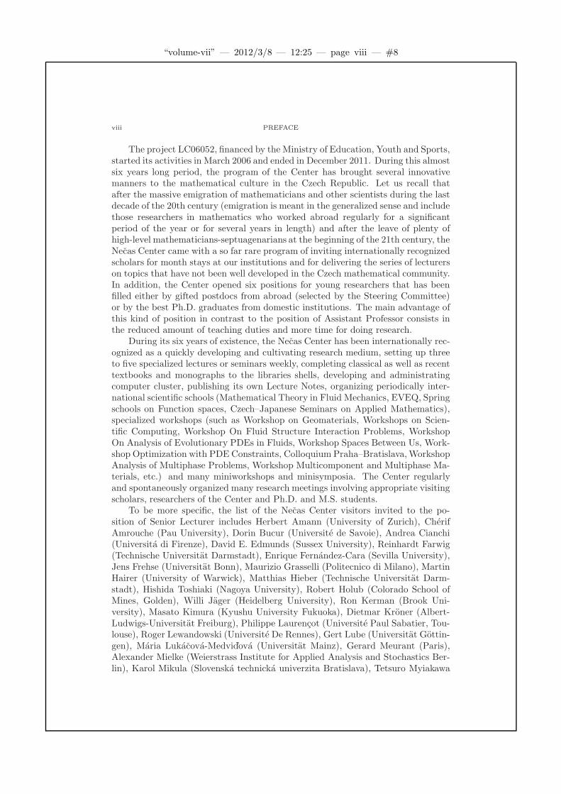
viii PREFACE

The project LC06052, financed by the Ministry of Education, Youth and Sports,started its activities in March 2006 and ended in December 2011. During this almostsix years long period, the program of the Center has brought several innovativemanners to the mathematical culture in the Czech Republic. Let us recall thatafter the massive emigration of mathematicians and other scientists during the lastdecade of the 20th century (emigration is meant in the generalized sense and includethose researchers in mathematics who worked abroad regularly for a significantperiod of the year or for several years in length) and after the leave of plenty ofhigh-level mathematicians-septuagenarians at the beginning of the 21th century, theNecas Center came with a so far rare program of inviting internationally recognizedscholars for month stays at our institutions and for delivering the series of lecturerson topics that have not been well developed in the Czech mathematical community.In addition, the Center opened six positions for young researchers that has beenfilled either by gifted postdocs from abroad (selected by the Steering Committee)or by the best Ph.D. graduates from domestic institutions. The main advantage ofthis kind of position in contrast to the position of Assistant Professor consists inthe reduced amount of teaching duties and more time for doing research.

During its six years of existence, the Necas Center has been internationally rec-ognized as a quickly developing and cultivating research medium, setting up threeto five specialized lectures or seminars weekly, completing classical as well as recenttextbooks and monographs to the libraries shells, developing and administratingcomputer cluster, publishing its own Lecture Notes, organizing periodically inter-national scientific schools (Mathematical Theory in Fluid Mechanics, EVEQ, Springschools on Function spaces, Czech–Japanese Seminars on Applied Mathematics),specialized workshops (such as Workshop on Geomaterials, Workshops on Scien-tific Computing, Workshop On Fluid Structure Interaction Problems, WorkshopOn Analysis of Evolutionary PDEs in Fluids, Workshop Spaces Between Us, Work-shop Optimization with PDE Constraints, Colloquium Praha–Bratislava,WorkshopAnalysis of Multiphase Problems, Workshop Multicomponent and Multiphase Ma-terials, etc.) and many miniworkshops and minisymposia. The Center regularlyand spontaneously organized many research meetings involving appropriate visitingscholars, researchers of the Center and Ph.D. and M.S. students.

To be more specific, the list of the Necas Center visitors invited to the po-sition of Senior Lecturer includes Herbert Amann (University of Zurich), CherifAmrouche (Pau University), Dorin Bucur (Universite de Savoie), Andrea Cianchi(Universita di Firenze), David E. Edmunds (Sussex University), Reinhardt Farwig(Technische Universitat Darmstadt), Enrique Fernandez-Cara (Sevilla University),Jens Frehse (Universitat Bonn), Maurizio Grasselli (Politecnico di Milano), MartinHairer (University of Warwick), Matthias Hieber (Technische Universitat Darm-stadt), Hishida Toshiaki (Nagoya University), Robert Holub (Colorado School ofMines, Golden), Willi Jager (Heidelberg University), Ron Kerman (Brook Uni-versity), Masato Kimura (Kyushu University Fukuoka), Dietmar Kroner (Albert-Ludwigs-Universitat Freiburg), Philippe Laurencot (Universite Paul Sabatier, Tou-louse), Roger Lewandowski (Universite De Rennes), Gert Lube (Universitat Gottin-gen), Maria Lukacova-Medvid’ova (Universitat Mainz), Gerard Meurant (Paris),Alexander Mielke (Weierstrass Institute for Applied Analysis and Stochastics Ber-lin), Karol Mikula (Slovenska technicka univerzita Bratislava), Tetsuro Myiakawa

“volume-vii” — 2012/3/8 — 12:25 — page ix — #9

PREFACE ix

(Kanazawa University), Antonın Novotny (University of Toulon), Patrick Rabier(University of Pittsburg), Hans-Gorg Roos (Dresden University), Roman Shvydkoy(University of Illinois, Chicago), Endre Suli (Oxford Univerzity), Daniel Sevcovic(Univerzita Komenskeho Bratislava), Peter Takac (Rostock University), WernerVarnhorn (Universitat Kassel), Wolfgang Wendland (Universitat Stuttgart), JorgWolf (Humboldt Universitat Berlin), Shigetoshi Yazaki (University of Miyazaki)and Ping Zhang (Chinese Academy of Sciences).

The list of foreign postdocs who took the position of Junior Researchers inthe Center include, among many others, Helmut Abels (currently full professorat University of Regensburg), Tomasz Cieslak, Lars Diening (currently full pro-fessor in Munchen), Luisa Consiglieri, Pierre-Etienne Druet, Jan Schneider, Yu-taka Terasawa, Guiseppe Tomasetti, Riccarda Rossi, Vladislav Mantic, Soren Bar-tels, Adrian Muntean, Mathieu Hillaret, Mark Steinhauer (currrently professorin Koblenz), Yongzhong Sun, Timofei Silkhin, Julia Namlyeyeva, Trygve Karper,Marita Thomas, Daniel Wachsmut, among others. At least for the period of sev-eral months these positions were gradually occupied by Jaroslav Hron, MiroslavBulıcek, Iveta Hnetynkova, Vaclav Kucera, Jirı Mikyska, Tomas Oberhuber, JanStebel, Vıt Prusa, Martin Lanzendorfer, Miloslav Vlasak and Ondrej Soucek.

The activities of the Necas Center have been in particular an inspiration for ayoung generation of Polish mathematicians (P. Gwiazda, P. Mucha and

A. Swierczewska-Gwiazda), the Center has strengthened the scientific as well aseducational cooperation between Prague mathematical school and schools in Hei-delberg and Darmstadt, the own existence of the Center further enhanced jointresearch programs with colleagues in Berlin, Regensburg, Paris, Toulon, Toulouse,Rome, Firenze, etc., and with members of Japanese and Chinese mathematical andengineering circles. Just to illustrate the atmosphere, after spending a month inthe Necas Center, Endre Suli writes: “I have been hugely impressed by the veryhigh standard of scientific life in the Necas Center. The existence of this center isvital for the future of Applied Mathematics in the Czech Republic and in particularin training future generations of excellent M.Sc. and Ph.D. students. Given theimportance of the field of Applied Mathematics in a wide range of application areas,including industry, economics, the life sciences, physical, chemical and engineeringsciences, and the Necas Center’s clear commitment to the understanding of dif-ficult mathematical problems with direct relevance to applications, the continuedexistence of the Necas Center seems paramount to me.”

We wish to thank all visitors, to the members of the Steering Committee as wellas particular members of research teams who contributed to whatever activities ofthe Center. In particular, we wish to underline the names of those who help us,in an extraordinary way, in advertising the Center abroad and in forming researchdirections. These are Willi Jager, Antonın Novotny, K. R. Rajagopal, ZdenekStrakos and Daniel Sevcovic.

The Necas Center, center for fundamental research, was focused on six followed-up, nevertheless different main goals that share a common feature, namely, a goal-oriented mergence of modern theoretical, numerical and computer approaches to-wards a solution of problems in particular thematic topics. The first goal wasfocused on problems describing mechanical processes in a single continuum, the

“volume-vii” — 2012/3/8 — 12:25 — page x — #10

x PREFACE

second and third goals consisted of solving problems involving in addition boththermal and chemical processes. The fourth goal concentrated on the theory ofinteracting continua (mixture theory, multiphase and multicomponent materials,role of boundary conditions). The fifth goal was to investigate the links betweenfull models and their approximations (based on nondimensional analysis and modelreduction). The last goal then integrated all the previous goals in a synthetic man-ner and culminated, in particular, by the preparation of several multidisciplinaryprojects based on these broad grounds. The output of the research is formed mostlyby scientific papers and developed software. More than 200 papers supported by theproject LC06052 were written in cooperation between members of various researchunits or in cooperation with visiting foreign guests.

Tremendous amount of activities and scientific results obtained in the Center,and its fundamental role in the growth of a new promising generation of youngresearchers suggest to evaluate this project as very successful. How successful theproject of the Necas Center was will be however fully evident much later. We stillhope that we will be capable of establishing the Necas Center as a research unitconnecting groups in the Academy of Sciences, Czech Technical University, CharlesUniversity and others with similar visions and complementary expertise. In such acenter—that may exist independently of any particular project—we wish to carry onand further enhance our experience built in the Center following the aim to establisha multidisciplinary mathematical environment opened towards cooperation withresearchers in the areas of natural and life sciences.

Prague, 31 January 2012Michal Benes

Eduard FeireislJosef Malek

“volume-vii” — 2012/3/8 — 12:25 — page xi — #11

Contents

Preface vii

Part 1. Weighted Sobolev spaces and elliptic problems in the

half-space

Cherif Amrouche 1

Chapter 1. Weighted Sobolev spaces and elliptic problems in the half-space 51. Introduction 52. Laplace equation in RN 63. Functional spaces 84. Spaces of traces and inequalities 95. The Dirichlet problem for the Laplacian in RN

+ 13

6. The biharmonic problem in RN+ 15

7. Stokes problem with Dirichlet or Navier boundary conditions 188. Elliptic systems with data in L1(RN

+ ) 22

Bibliography 25

Part 2. Generalised trigonometric functions, compact operators and

the p-LaplacianDavid E. Edmunds 27

Chapter 1. Generalised trigonometric functions, compact operators and thep−Laplacian 31

1. Introduction 312. The p−trigonometric functions 323. Representation of compact linear operators 37

Bibliography 47

Part 3. The control of PDEs: some basic concepts, recent results

and open problems

Enrique Fernandez-Cara 49

Chapter 1. Optimal control of systems governed by PDEs 531. Some examples 532. Existence, uniqueness and optimality results 563. Control on the coefficients, nonexistence and relaxation 614. Optimal design and domain variations 63

xi

“volume-vii” — 2012/3/8 — 12:25 — page xii — #12

xii CONTENTS

5. Optimal control for a system modelling tumor growth 67

Chapter 2. Controllability of the linear heat and wave PDEs 691. Introduction 692. Basic results for the linear heat equation 703. Basic results for the linear wave equation 78

Chapter 3. Controllability results for other time-dependent PDEs 831. Introduction. Recalling general ideas 832. The heat equation. Observability and Carleman estimates 843. Some remarks on the controllability of stochastic PDEs 884. Positive and negative results for the Burgers equation 935. The Navier-Stokes and Boussinesq systems 946. Some other nonlinear systems from mechanics 97

Bibliography 101

Part 4. Fluid-structure interaction for shear-dependent non-

Newtonian fluids

Anna Hundertmark-Zauskova, Maria Lukacova-Medvidova,

Gabriela Rusnakova 109

Chapter 1. Fluid-structure interaction methods 1131. Introduction 1132. Mathematical model for shear-dependent fluids 1143. Generalized string model for the wall deformation 1174. Fluid-structure interaction methods 121

Chapter 2. Numerical study 1311. Numerical study 1312. Concluding remarks 153

Bibliography 155

Part 5. Analysis in Orlicz spaces

Ron Kernan 159

Chapter 1. Analysis in Orlicz spaces 1631. Introduction 1632. The Orlicz class LΦ(Ω) 1653. The completeness of LΦ(Ω) 1704. Duality 1715. The rearrangement invariance of LΦ(Ω) 1756. The role of Orlicz spaces in the theory of elliptic PDE 178

Bibliography 185

Part 6. Topics in the Q-tensor theory of liquid crystals

Arghir Zarnescu 187

“volume-vii” — 2012/3/8 — 12:25 — page xiii — #13

CONTENTS xiii

Chapter 1. Mathematical modelling 1911. Some history and the main physical aspects 1912. The probability distribution function and the Q-tensor 1933. Some simple properties of Q-tensors 1964. A Q-tensor model: the Beris-Edwards system 1985. Defect patterns and their diverse descriptions 200

Chapter 2. Qualitative features of a stationary problem: Oseen–Frank limit 2031. Preliminaries 2042. The limiting harmonic map and the uniform convergence 2063. Biaxiality and uniaxiality 220

Chapter 3. Well-posedness of a dynamical model: Q-tensors andNavier–Stokes 231

1. The dissipation and apriori estimates 2312. Weak solutions 2343. Strong solutions 238

Bibliography 243

Appendix A. Representations of Q and the biaxiality parameter β(Q) 247

Appendix B. Properties of the bulk term fB(Q) 251

“volume-vii” — 2012/3/8 — 12:25 — page xiv — #14

“volume-vii” — 2012/3/8 — 12:25 — page 1 — #15

Part 1

Weighted Sobolev spaces and

elliptic problems in the half-space

Cherif Amrouche

“volume-vii” — 2012/3/8 — 12:25 — page 2 — #16

2000 Mathematics Subject Classification. 35D05, 35D10, 35J05, 35J25, 35J55,76D03, 76D07

Key words and phrases. Laplace equation, biharmonic problem, Stokes problem,weighted Sobolev spaces, traces, reflection principle, half-space

Abstract. In this paper, we study the Laplace equation in the whole spaceand we give some properties concerning the functions which belong to weightedSobolev spaces and their traces. We prove in Lp theory, with 1 < p < ∞

some existence and uniqueness results concerning the Laplace equation, thebiharmonic problem and the Stokes problem in the half-space RN

+, with N > 2

and with Dirichlet boundary conditions or with Navier boundary conditionsin the case of Stokes problem. Finally, we investigate the case of data in L1.

“volume-vii” — 2012/3/8 — 12:25 — page 3 — #17

Contents

Chapter 1. Weighted Sobolev spaces and elliptic problems in the half-space 51. Introduction 52. Laplace equation in RN 63. Functional spaces 84. Spaces of traces and inequalities 94.1. Case W 1,2

0 (RN+ ). 9

4.2. Case W 1,p0 (RN

+ ). 114.3. General Case 125. The Dirichlet problem for the Laplacian in RN

+ 13

6. The biharmonic problem in RN+ 15

7. Stokes problem with Dirichlet or Navier boundary conditions 188. Elliptic systems with data in L1(RN

+ ) 22

Bibliography 25

3

“volume-vii” — 2012/3/8 — 12:25 — page 4 — #18

“volume-vii” — 2012/3/8 — 12:25 — page 5 — #19

CHAPTER 1

Weighted Sobolev spaces and elliptic problems in

the half-space

1. Introduction

We will study here the following elliptic problems: the Laplace equation withDirichlet or Neumann boundary condition:

(L)

−∆u = f in RN

+ = x ∈ RN ; xN > 0,u = g0 or ∂Nu = g1 on Γ ≡ RN−1 × 0,

the biharmonic problem with Dirichlet boundary condition:

(B)

∆2u = f in RN

+ ,u = g0 and ∂Nu = g1 on Γ,

the Stokes system with Dirichlet or Navier boundary condtion

(S)

−∆u+∇π = f and divu = h in R

N+ ,

u = g or uN = gN and ∂Nu′ = g′ on Γ.

We are also interested in Laplace’s system with right hand side in L1:

(L)

−∆u = f in R

N+ ,

u = g or ∂Nu = g on Γ.

Question 1 : What is the functional setting to use Lax-Milgram Lemma for theproblem:

−∆u = f in RN+ , u = g on Γ ?

Considering the case g = 0, it is then clear that the solution must satisfy:

∇u ∈ L2(RN+ ).

We observe that the solution does not belong to L2(RN+ ), hence the classical Sobolev

space H1(RN+ ) is not suited. Also, the trace of function such that ∇u ∈ L2(RN

+ ) is

not in H1/2(RN−1).

Question 2 : What about the case f ∈ L1(RN+ ) or g ∈ L1(Γ)?

The Stokes problem in the half-space was studied by [4, 8, 10, 14, 16, 17, 19,20, 21]. More recently, Laplace’s equation, with estimates for L1 vector fields wasstudied by [5, 11, 12, 13].

5

“volume-vii” — 2012/3/8 — 12:25 — page 6 — #20

6 1. WEIGHTED SOBOLEV SPACES AND ELLIPTIC PROBLEMS IN THE HALF-SPACE

2. Laplace equation in RN

We will consider the following Laplace equation (see [2] for more details):

−∆u = f in RN . (1.1)

Variational Formulation: Find u ∈ V such that

∀v ∈ V,

∫

RN

∇u · ∇v = < f, v >,

where

V = v ∈ D′(RN ); ∇v ∈ L2(RN ).But we must bring V with an Hilbertian space structure.

Lemma 1.1. Let 1 < p <∞ and v ∈ D′(RN ) such that ∇v ∈ Lp(RN ).

(i) If p < N , then there exists a unique constant K such that v+K|x| ∈ Lp(RN ),

with the estimate∥∥v +K

|x|∥∥Lp(RN )

≤ C‖∇v‖Lp(RN )

(ii) If p > N , then v|x| ∈ Lp(RN ), with the estimate

infµ∈R

∥∥v + µ

|x|∥∥Lp(RN )


(iii) If p = N , then v|x|ln(1+|x|) ∈ Lp(RN ), with the estimate

infµ∈R

∥∥ v + µ

|x|ln(1 + |x|)∥∥Lp(RN )


where C > 0 is a constant depending only on p and N .

Proof. Because, we are interested here mainly in the behavior at the infinity,we will replace |x| = r by 1 + r. We set

W 1,p0 (RN ) = u ∈ D′(RN ),

u

w0∈ Lp(RN ),∇u ∈ Lp(RN ),

where

w0 = 1 + r if p 6= N, w0 = (1 + r) ln(2 + r) if p = N.

We use then the Hardy inequalities: for any v ∈ W 1,p0 (RN ),

∥∥ vw0

∥∥Lp(RN )

≤ C‖∇v‖Lp(RN ) if p < N,

and

Infµ∈R

∥∥v + µ

w0

∥∥Lp(RN )

≤ C‖∇v‖Lp(RN ) if p ≥ N.

We deduce that the range of the gradient operator:

grad : W 1,p0 (RN ) 7→ Lp(RN )⊥ Hp′(RN ),

with

Hp′(RN ) =ϕ ∈ Lp′

(RN ); divϕ = 0,

“volume-vii” — 2012/3/8 — 12:25 — page 7 — #21

2. LAPLACE EQUATION IN RN 7

is a closed subspace of Lp′

(RN ). Here, Lp(RN )⊥ Hp′(RN ) denotes the subspaceof functions f in Lp(RN ) which satisfy < f , v >= 0 for any v ∈ Hp′(RN ). Letv ∈ D′(RN ) such that ∇v ∈ Lp(RN ). By the density of

V(RN ) = ϕ ∈ D(RN ); divϕ = 0 in the space Hp′(RN ), we deduce that ∇v ∈ Lp(RN )⊥ Hp′(RN ) and then there

exists w ∈ W 1,p0 (RN ) such that ∇w = ∇v and then there exists a unique constant

K such that w = v +K.

Return to the variational formulation of the Laplace equation. The good choiceof the space V is given by the space W 1,2

0 (RN ). We denote by

W−1,p′

0 (RN ) = [W 1,p0 (RN )]′.

For the general case 1 < p <∞, we have then

Theorem 1.2. Let f ∈ W−1,p0 (RN ), with 1 < p < ∞, satisfying the compati-

bility condition

< f, 1 >= 0 if p ≤ N

N − 1. (1.2)

Then, there exists a unique u ∈ W 1,p0 (RN ), up to a constant if p ≥ N , satisfying

(1.1) and the corresponding estimate. Moreover, if p < N , then u = E ⋆ f , whereE is the fundamental solution of the Laplacian.

Proof. Thanks to Hardy inequality, we write f = div v, with v ∈ Lp(RN ).Let vm ∈ D(RN ) such that vm −→ v in Lp(RN ). Setting fm = div vm andψm = E ⋆ fm. We have for any ϕ ∈ D(RN ),

< ∂iψm, ϕ > = − < E ⋆ fm, ∂iϕ > = < vm, ∇∂i(E ⋆ ϕ) > .

According to Calderon-Zygmund inequality, we obtain:

| < ∂iψm, ϕ > | ≤ ‖vm‖Lp(RN )‖∇∂i(E ⋆ ϕ)‖Lp′(RN )

≤ C‖vm‖Lp(RN )‖∆(E ⋆ ϕ)‖Lp′(RN )

≤ C‖f‖W−1,p0 (RN )‖ϕ‖Lp′(RN ),

so that∇ψm is bounded inLp(RN ) and there exists a sequence cm such that ψm+cmconverges weakly to some function u in W 1,p

0 (RN ) and −∆u = f .

To study some regularity results, we need to define the following weightedspaces:

W 2,p1 (Ω) = u ∈ D′(Ω),

u

w0∈ Lp(Ω),∇u ∈ Lp(Ω), w2D

2u ∈ Lp(Ω),

where

w0 = 1 + r if p 6= N, w0 = (1 + r) ln(2 + r) if p = N, w2 = 1 + r.

and

W 0,p1 (RN ) = u ∈ D′(RN ), (1 + r)u ∈ Lp(RN ).

Note that W 2,p1 (Ω) →W 1,p

0 (RN ) and

W 0,p1 (RN ) → W−1,p

0 (RN ) ⇔ N 6= p′

“volume-vii” — 2012/3/8 — 12:25 — page 8 — #22


Corollary 1.3. Let

f ∈W 0,p1 (RN ) if N 6= p′ or f ∈ W−1,p

0 (RN ) ∩W 0,p1 (RN ) if N = p′

and satisfy the compatibility condition (1.2). Then, the solutions given by the pre-

vious theorem belong to W 2,p1 (RN ) and we have the following weighted Calderon-

Zygmund inequality: for any ϕ ∈ D(RN )

‖(1 + |x|) ∂2ϕ

∂xi∂xj‖Lp(RN ) ≤ ‖(1 + |x|)∆ϕ‖Lp(RN )

if and only if N 6= p′.

To find another strong solutions, with another behavior at the infinity, we set

W 2,p0 (RN ) = u ∈ D′(Ω),

u

w0∈ Lp(Ω),

∇uw1

∈ Lp(Ω), D2u ∈ Lp(Ω),

where

w0 = (1 + r)2 if p /∈ N2, N, w0 = (1 + r)2 ln(2 + r) otherwise,


Theorem 1.4.

(i) Let f ∈ Lp(RN ). Then, there exists a unique u ∈ W 2,p0 (RN ), up to a poly-

nomial of degre less or equal 1 if p ≥ N , up to a constant if N2 ≤ p < N ,

satisfying (1.1). Moreover, if p < N2 , then u = E ⋆ f , where E is the funda-

mental solution of the Laplacian.

(ii) Let f ∈ W−2,p0 (RN ) and satisfy the compatibility condition

< f, 1 >=< f, xi >= 0 if p ≤ N

N − 1and < f, 1 >= 0 if

N

N − 1< p ≤ N

N − 2.

Then, there exists a unique solution u ∈ Lp(RN ) satisfying (1.1).

3. Functional spaces

More generally, we define the following weighted Sobolev spaces (see [2] formore details). Let m ∈ N, α, β ∈ R, p ∈ ]1,∞[, Ω any open set of RN ,

Wm, pα, β (Ω) =

u ∈ D′(Ω) ; 0 6 |λ| 6 k, α−m+|λ| (lg )β−1 ∂λu ∈ Lp(Ω) ;

k + 1 6 |λ| 6 m, α−m+|λ| (lg )β ∂λu ∈ Lp(Ω),

where = (1 + |x|2)1/2, lg = ln(1 + 2), λ ∈ NN ,

and k =

−1 if Np + α /∈ 1, . . . ,m,

m− Np − α if N

p + α ∈ 1, . . . ,m.If β = 0, we simply denote this space by Wm, p

α (Ω) and we set

W

m, pα, β (Ω) = D(Ω)

‖·‖W

m, pα, β

(Ω) and W−m, p′

−α,−β(Ω) =( W

m, pα, β (Ω)

)′.

“volume-vii” — 2012/3/8 — 12:25 — page 9 — #23

4. SPACES OF TRACES AND INEQUALITIES 9

Example 1.5 (Examples of Weighted Sobolev Spaces).

W 1,p0 (Ω) = u ∈ D′(Ω),

u

w0∈ Lp(Ω),∇u ∈ Lp(Ω),

where


W 2,p0 (Ω) = u ∈ D′(Ω),

u

w0∈ Lp(Ω),

∇uw1

∈ Lp(Ω), D2u ∈ Lp(Ω),where

w0 = (1 + r)2 if p /∈ N2, N, w0 = (1 + r)2 ln(2 + r), otherwise,

and


W 2,p1 (Ω) = u ∈ D′(Ω),

u

w0∈ Lp(Ω),∇u ∈ Lp(Ω), w2D

2u ∈ Lp(Ω),where

w0 = 1 + r if p 6= N, w0 = (1 + r) ln(2 + r) if p = N,

w2 = 1 + r.

4. Spaces of traces and inequalities

In this section, we give some properties concerning the functions which belongto weighted Sobolev spaces and their traces (see [1, 3]).

4.1. Case W 1,20 (RN

+ ). We consider the space:

W1/2,20 (RN−1) = u ∈ D′(RN−1) ;

u

ω′1/2 ∈ L2(RN−1),∫

RN−1× RN−1

|u(x′)− u(y′)|2|x′ − y′|N dx′dy′ <∞,

with ω′ = ′ = (1 + |x′|2)1/2 if N ≥ 3 and ω′ = ′(lg′)2 if N = 2. It is a reflexiveBanach for the norm:

||u||W

1/2,20 (RN−1)

=(∫

RN−1

|u(x′)|2ω′ dx′ +

∫

RN−1× RN−1

|u(x′)− u(y′)|2|x′ − y′|N dx′dy′

)1/2.

Its semi-norm:

|u|W

1/2,20 (RN−1)

=(∫

RN−1× RN−1

|u(x′)− u(y′)|2|x′ − y′|N dx′dy′

)1/2.

Lemma 1.6. For any N ≥ 2 and u ∈ D(RN−1), we have the relation∫

RN−1× RN−1

|u(x′)− u(y′)|2|x′ − y′|N dx′dy′ = CN

∫

RN−1

|ξ′||u(ξ′)|2dξ′

On D(RN−1), the semi-norms | · |W

1/2,20 (RN−1)

and | · |H1/2(RN−1) are equivalent,

where H1/2(RN−1) is the classical Sobolev space which corresponds to the traces offunctions in H1(RN

+ ).

By Fourier’s transform, it is easy to prove the following lemma:

“volume-vii” — 2012/3/8 — 12:25 — page 10 — #24


Lemma 1.7. For any N ≥ 2 and u ∈ D(RN

+

), we have the inequality

∫

RN−1

|ξ′| |u(ξ′, 0)|2 dξ′ ≤ C

∫

RN+

|∇u|2dx,

that means that

∀u ∈ D(RN

+

), | γ0(u) |W 1/2,2

0 (RN−1)≤ C|u|W 1,2

0 (RN+ ).

Recall now the Pitt’s Inequality. For any N ≥ 3 and u ∈ D(RN−1), we have :∫

RN−1

|u(ξ′)|2|ξ′| dξ′ ≤ C

∫

RN−1

|ξ′| |u(ξ′)|2 dξ′.

If N = 2, we can prove the following lemma:

Lemma 1.8. For any u ∈ D(]0,∞[), we have :∫ ∞

0

|u(t)|2t ln2(2 + t)

dt ≤ C

∫ ∞

0

∫ ∞

0

|u(t)− u(τ)|2|t− τ |2 dtdτ.

As consequence of the previous lemmas, we can prove

Theorem 1.9.

(i) If N ≥ 3, for any u ∈W 1,20 (RN

+ ), we have:∫

RN−1

|γ0u(x′)|2|x′| dx′ ≤ C1

∣∣ γ0u∣∣W

1/2,20 (RN−1)

≤ C2|u|W 1,20 (RN

+ ).

(ii) If N = 2, for any u ∈W 1,20 (R2

+), we have:

infK∈R

∫

R

|γ0u(x1) +K|2|x1| ln2(2 + |x1|)

dx1 ≤ C1

∣∣ γ0u∣∣W

1/2,20 (RN−1)

≤ C2|u|W 1,20 (RN

+ ).

(iii) If N ≥ 2, the mapping γ0 : u ∈ D(RN+ ) → γ0u ∈ D(RN−1) can be extended to a

linear continuous mapping denoted by γ0 from W 1,20 (RN

+ ) into W1/2,20 (RN−1).

The lifting operator in W1/2,20 (RN−1) is given by the following lemma.

Lemma 1.10. Let N ≥ 2 and g ∈ W1/2,20 (RN−1). Then, there exists u = Rg ∈

W 1,20 (RN

+ ) such that u = g on RN−1 and

||u||W 1,20 (RN

+ ) ≤ C|g|W

1/2,20 (RN−1)

if N ≥ 3,

infK∈R

||u+K||W 1,20 (R2

+) ≤ C|g|W

1/2,20 (RN−1)

if N = 2.

A variant of the last inequality:

Lemma 1.11. For any g ∈W1/2,20 (R) such that∫ 1

−1

g(t)dt = 0,

“volume-vii” — 2012/3/8 — 12:25 — page 11 — #25

4. SPACES OF TRACES AND INEQUALITIES 11

there exists u = Rg ∈W 1,20 (R2

+) such that u = g on R and

||u||W 1,20 (R2

+) ≤ C||g||W

1/2,20 (R)

.

We can now summarize:

Theorem 1.12. Let N ≥ 2. The mapping

γ0 : u ∈W 1,20 (RN

+ ) → γ0u ∈W1/2,20 (RN−1)

is continuous, surjective and Ker γ0 =W

1,2

0 (RN+ ).

4.2. Case W 1,p0 (RN

+ ). We consider the space:

W1−1/p,p0 (RN−1) =

u ∈ D′(RN−1) ;

u

ω′1−1/p∈ Lp(RN−1),

∫

RN−1× RN−1

|u(x′)− u(y′)|p|x′ − y′|N+p−2

dx′dy′ <∞,

with

ω′ = ′ = (1 + |x′|2)1/2 if N 6= p and ω′ = ′(lg′)2 if N = p.

It is a reflexive Banach with the norm ||u||W

1−1/p,p0 (RN−1)

:

(∫

RN−1

|u(x′)|pω′p−1

dx′ +

∫

RN−1× RN−1

|u(x′)− u(y′)|p|x′ − y′|N+p−2

dx′dy′)1/p

.

Its semi-norm is defined by

|u|W

1−1/p,p0 (RN−1)

=( ∫

RN−1×RN−1

|u(x′)− u(y′)|p|x′ − y′|N+p−2

)1/p

Lemma 1.13. Let N ≥ 2 and 1 < p < ∞. Then for any u ∈ D(RN+ ), we have

the inequality∫

RN−1× RN−1

|u(x′, 0)− u(y′, 0)|p|x′ − y′|N+p−2

dx′dy′ ≤ C

∫

RN+

|∇u|pdx,

that means that the semi-norm in RN−1 is controlled by the semi-norm in the whole

space.

Recall now the Pitt’s Inequality. For any N ≥ 3, 1 < p < N and u ∈ D(RN−1),we have the inequality

∫

RN−1

|u(ξ′)|p|ξ′|p−1

dξ′ ≤ C

∫

RN−1

|ξ′|pN−2N+1 |u(ξ′)|p dξ′.

Corollary 1.14. For any N ≥ 2, u ∈ D(RN+ ) and 1 < p ≤ 2, we have the

inequalities:∫

RN−1

|u(ξ′, 0)|p|ξ′|p−1

dξ′ ≤ C1

∫

RN−1× RN−1

|u(x′, 0)− u(y′, 0)|p|x′ − y′|N+p−2

≤ C2

∫

RN+

|∇u|pdx,

“volume-vii” — 2012/3/8 — 12:25 — page 12 — #26


that means that

|γ0u|W 0,p1/p−1

(RN−1) ≤ C1|γ0u|W 1−1/p,p0 (RN−1)

≤ C2|u|W 1,p0 (RN

+ )

What is the analogue of this result when 2 < p < N? We will use an interpo-lation argument.

Proposition 1.15. For any 1 < p < N and any u ∈ W1−1/p,p0 (RN−1), we

have the estimates ∫

RN−1

|u(x)|p|x|p−1

dx ≤ C|u|W

1−1/p,p0 (RN−1)

.

Remark 1.16. See [18] for an another proof.

Corollary 1.17. Let 1 < p < N . Then for any u ∈ W 1,p0 (RN

+ ), we have theestimates:

|γ0u|W 0,p1/p−1

(RN−1) ≤ C1|γ0u|W 1−1/p,p0 (RN−1)

≤ C2|u|W 1,p0 (RN

+ )

When the exponent p is greater or equal to the dimension N , we have:

Lemma 1.18.

(i) Let p > N . Then for any u ∈ W 1,p0 (RN

+ ), we have the estimates:

infK∈R

|γ0u+K|W 0,p1/p−1

(RN−1) ≤ C|u|W 1,p0 (RN

+ ).

(ii) If p = N and u ∈ W 1,N0 (RN

+ ), we have the estimates:

infK∈R

∫

RN−1

|γ0u(x′) +K|N|x′|N−1 lnN (2 + |x′|)

dx′ ≤ C|u|W 1,N0 (RN

+ ).

As for the Hilbertian case, we have:

Theorem 1.19. Let N ≥ 2. The following mapping

γ0 : u ∈ D(RN+ ) → γ0u ∈ D(RN−1)

can be extended to a linear continuous mapping denoted also γ0 from W 1,p0 (RN

+ )

into W1−1/p,p0 (RN−1). Moreover γ0 is onto and Ker γ0 =

W

1,p0 (RN

+ ).

4.3. General Case. We consider the following spaces of traces.

For anyσ ∈ ]0, 1[,

W σ, pα (RN ) =

u ∈ D′(RN ) ; ωα−σu ∈ Lp(RN ),

∫

RN×RN

|α(x)u(x) − α(y)u(y)|p|x− y|N+σp

dx dy <∞,

where ω = if N/p+ α 6= σ and ω = (lg )1/(σ−α) if N/p+ α = σ.

For any s ∈ R+,

W s, pα (RN ) =

u ∈ D′(RN ) ; 0 6 |λ| 6 k, α−s+|λ| (lg )−1 ∂λu ∈ Lp(RN ) ;

k + 1 6 |λ| 6 [s]− 1, α−s+|λ| ∂λu ∈ Lp(RN ) ; |λ| = [s], ∂λu ∈W σ, pα (RN )

,

“volume-vii” — 2012/3/8 — 12:25 — page 13 — #27

5. THE DIRICHLET PROBLEM FOR THE LAPLACIAN IN RN+ 13

where k = s−N/p− α if N/p+ α ∈ σ, . . . , σ + [s], with σ = s− [s] and k = −1otherwise.

We have the following general result (see [3]):

Lemma 1.20. The mapping γ = (γ0, γ1, . . . , γm−1) : D(RN

+

)−→ D(RN−1)

m,

can be extended by continuity to a linear and continuous mapping:

γ : Wm, pα (RN

+ ) −→m−1∏

j=0

Wm−j−1/p, pα (RN−1).

Moreover, γ is onto and Ker γ =Wm, p

α (RN+ ).

Let us now introduce the following spaces of polynomials. For q ∈ Z, Pq isthe space of polynomials of degree 6 q, P∆

q the subspace of harmonic polynomials

of Pq, P∆2

q the subspace of biharmonic polynomials of Pq, A∆q is the subspace of

polynomials P∆q , odd with respect xN , N∆

q is the subspace of polynomials P∆q ,

even with respect xN . Observe that ϕ ∈ A∆q ⇔ ϕ(x′, 0) = 0 and ϕ ∈ N∆

q ⇔∂Nϕ(x

′, 0) = 0. For all s ∈ R, [s] denotes a real part of s.

5. The Dirichlet problem for the Laplacian in RN+

We consider the following Dirichlet problem for the Laplacian in the half-space(see [3]):

(PD) ∆u = f in RN+ u = g on Γ := R

N−1 × 0.We recall that Aq

∆ is the subspace of polynomials Q of Pq∆ satisfying Q(x′, 0) = 0.

Theorem 1.21. Let ℓ ≥ 0 be an integer and Np′ /∈ 1, . . . , ℓ with the convention

this set is empty if ℓ = 0. For any f in W−1,pℓ (RN

+ ) and g in W1p′

,p

ℓ (Γ) satisfyingthe compatibility condition

∀ϕ ∈ A[ℓ+1−Np′

]∆ , < f, ϕ >

W−1,pℓ

×W 1,p′

−l

= < g,∂ϕ

∂xN>Γ,

where < ·, · >Γ denote the duality brackets between W1p′

,p

ℓ (Γ) and W− 1

p′,p

−ℓ (Γ), prob-

lem (PD) has a unique solution u ∈ W 1,pℓ (RN

+ ) and

||u||W 1,pℓ (RN

+ ) ≤ C(||f ||W−1,pℓ (RN

+ ) + ||g||W

1p′

,p

ℓ (Γ)).

Proof. Note that the kernel of the operator

(−∆, γ0) :W 1,pℓ (RN

+ ) → W−1,pℓ (RN

+ )×W1p′

,p

ℓ (Γ)

is precisely A∆[−ℓ+1−N/p′] for any integer ℓ and A∆

[−ℓ+1−Np′

]= 0 if ℓ ≥ 0. Let

ug ∈ W 1,pℓ (RN

+ ) be a lifting function of g:

ug = g on Γ and ||ug||W 1,pℓ (RN

+ ) ≤ C1||g||W

1p′

,p

ℓ (Γ).

Then, (PD) is equivalent to the problem

−∆v = f +∆ug in RN+ , v = 0 on Γ.

“volume-vii” — 2012/3/8 — 12:25 — page 14 — #28


Let h = f +∆ug. For any ϕ ∈W 1,p′

−ℓ (RN ), we set

⊓ϕ(x′, xN ) = ϕ(x′, xN )− ϕ(x′,−xN ) if xN > 0.

It is clear that ⊓ϕ ∈W 1,p′

−ℓ (RN+ ). Then h can be extended to hπ ∈ W−1,p

l (RN )defined by

ϕ ∈ W 1,p′

−ℓ (RN ), hπ(ϕ) = < h,⊓ϕ >W−1,p

ℓ (RN+ )×W 1,p′

−ℓ (RN+ ).

Moreover,

||hπ||W−1,pℓ (RN ) = ||h||W−1,p

ℓ (RN+ ).

Let q ∈ P∆[ℓ+1−N/p′]. Then,

q = r + s, r ∈ A∆[ℓ+1−N/p′] and s ∈ N∆

[ℓ+1−N/p].

So,

< hπ, q >= < f +∆ug, r >W−1,pℓ (RN

+ )×W 1,p′

−ℓ (RN+ )

and applying the Green formula:

< ∆ug, r >= −∫

RN+

∇ug · ∇rdx = −⟨g,

∂r

∂xN

⟩

W1p′

,p

ℓ (Γ)×W

−1p′

,p′

−ℓ (Γ)

(note that ∆r = 0 in RN+ and r = 0 on Γ). Then, hπ ∈ W−1,p

ℓ (RN ) and

∀q ∈ P∆[ℓ+1−N/p′], < hπ, q >= 0.

Recall that the operator

∆ :W 1,pℓ (RN ) → W−1,p

ℓ ⊥P∆[ℓ+1−N

p′]

if ℓ ≥ 1

and

∆ :W 1,p0 (RN )/P[1−N

p ] →W−1,p0 (RN )⊥P[1−N

p′] if ℓ = 0

are isomorphisms. Then, there exists v ∈W 1,pℓ (RN ) such that

−∆v = hπ.

Now, remark that the function w = 12 ⊓ v ∈ W 1,p

ℓ (RN+ ) and

−∆w = h in RN+ and w = 0 on Γ,

i.e. w is solution of our problem.

Remark 1.22.

(i) The kernel A∆[−l+1−N/p] is reduced to 0 if ℓ ≥ 0 and to P[1−N/p] if ℓ = 0.

(ii) With similar arguments, we can show an analogous result if ℓ < 0 :

f ∈W−1,pℓ (RN

+ ), g ∈W1p′

,p

ℓ (Γ),

then

u ∈ W 1,pℓ (RN

+ )/A∆[−ℓ+1−N/p].

“volume-vii” — 2012/3/8 — 12:25 — page 15 — #29

6. THE BIHARMONIC PROBLEM IN RN+ 15

6. The biharmonic problem in RN+

We are interested here by the biharmonic problem (see [6, 7, 8, 10, 15]):

(B)

∆2u = f in RN+ ,

u = g0 on Γ,

∂Nu = g1 on Γ.

As for Problem (PD), we have the following theorem.

Theorem 1.23 (Generalized solutions). Let ℓ ∈ Z be such that Np′ /∈ 1, . . . , ℓ

and Np /∈ 1, . . . ,−ℓ. There exists C > 0 such that for all f ∈ W−2, p

ℓ (RN+ ),

g0 ∈W2−1/p, pℓ (Γ) and g1 ∈ W

1−1/p, pℓ (Γ) satisfying the compatibility condition

∀ϕ ∈ B[2+ℓ−N/p′] : 〈f, ϕ〉W−2, p

ℓ (RN+ )×

W

2, p′

−ℓ (RN+ )

+ 〈g1,∆ϕ〉Γ − 〈g0, ∂N∆ϕ〉Γ = 0,

there exists a unique u ∈ W 2, pℓ (RN

+ )/B[2−ℓ−N/p] solution to (B), with the estimate

infq∈B[2−ℓ−N/p]

‖u+ q‖W 2, pℓ (RN

+ ) 6 C(‖f‖W−2, pℓ

+ ‖g0‖W 2−1/p, pℓ

+ ‖g1‖W 1−1/p, pℓ

).

Proof. First, we recall the reflection principle for ∆2. If u ∈ D′(RN+ ) is such

that ∆2u = 0, then u ∈ C∞(RN+ ).

Let u be a biharmonic function in RN+ with u = ∂Nu = 0 on Γ. Then, by the

Schwarz reflection principle, u can be extended uniquely by

u(x′, xN ) =

u(x′, xN ) if xN > 0,

(−u− 2xN∂Nu− x2N∆u)(x′,−xN ) if xN < 0.

to a biharmonic function on RN (see [15]). Now, if u ∈ W 2, pℓ (RN

+ ), we show that

u ∈ S ′(RN ) and then u ∈ P∆2

. Consequently,

Ker(∆2, γ0, γ1) = B[2−ℓ−N/p] =u ∈ P∆2

[2−ℓ−N/p] ; u = ∂Nu = 0 on Γ

with

(∆2, γ0, γ1) :W2, pℓ (RN

+ ) −→ W−2, pℓ (RN

+ )×W2−1/p, pℓ (Γ)×W

1−1/p, pℓ (Γ).

To prove the existence of solutions, we first consider the homogeneous problemcorresponding to f = 0:

(P 0)

∆2u = 0 in RN+ ,

u = g0 on Γ,

∂Nu = g1 on Γ.

We solve successively (see Amrouche-Necasova (2001) and Amrouche (2002))

(R0)

∆ϑ = 0 in R

N+ ,

ϑ = g0 on Γ,and (S0)

∆ζ = 0 in R

N+ ,

∂Nζ = g1 on Γ.

Then

u = xN ∂N (ζ − ϑ) + ϑ ∈W 1, pℓ−1(R

N+ )

satisfies (P 0) and we can show that u ∈W 2, pℓ (RN

+ ).

“volume-vii” — 2012/3/8 — 12:25 — page 16 — #30


For the complete problem, we use lifting of the boundary conditions:

∃ug ∈W 2, pℓ (RN

+ ), (ug, ∂Nug) = (g0, g1) on Γ.

If we put h = f−∆2ug ∈W−2, pℓ (RN

+ ) and v = u−ug, the problem (P ) is equivalentto the following problem:

(P ⋆)

∆2v = h in RN+ ,

v = 0 on Γ,∂Nv = 0 on Γ,

with h ⊥ B[2+ℓ−N/p′]. To solve the problem (P ⋆), we will prove that

∆2 :W

2, pℓ (RN

+ )/B[2−ℓ−N/p]) −→W−2, pℓ (RN

+ ) ⊥ B[2+ℓ−N/p′]

is an isomorphism.

Step 1. Case 2 + ℓ − N/p′ < 0. Let h ⊥ B[2+ℓ−N/p′]. Then h = div divH with

H ∈W 0, pℓ (RN

+ )N2

. We extend H by zero and set h = div div H. We know that there

exists z ∈ W 2, pℓ (RN ) satisfying ∆2z = h in RN . Setting z = z|RN

+∈ W 2, p

ℓ (RN+ ),

there exists w ∈ W 2, pℓ (RN

+ ) satisfying

∆2w = 0 in RN+ , w = z and ∂Nw = ∂Nz on Γ.

Then v = z − w answers to (P ⋆).

Step 2. Case 2− ℓ−N/p < 0. We deduce the result by duality from the previouscase, because ∆2 is selfadjoint.

Step 3. We finish by the case 2+ ℓ−N/p′ > 0 and 2− ℓ−N/p> 0 which impliesthat ℓ ∈ −1, 0, 1.

In the next theorem, we obtain strong solutions which are regular when thedata are also regular.

Theorem 1.24. Let ℓ ∈ Z, m ∈ N be such that

N

p′/∈ 1, . . . , ℓ+minm, 2 and

N

p/∈ 1, . . . ,−ℓ−m.

There exists C > 0 such that for all f ∈ Wm−2, pm+ℓ (RN

+ ), g0 ∈ Wm+2−1/p, pm+ℓ (Γ) and

g1 ∈Wm+1−1/p, pm+ℓ (Γ) satisfying the compatibility condition

∀ϕ ∈ B[2+ℓ−N/p′] : 〈f, ϕ〉W−2, p

ℓ (RN+ )×

W

2, p′

−ℓ (RN+ )

+ 〈g1,∆ϕ〉Γ − 〈g0, ∂N∆ϕ〉Γ = 0,

there exists a unique u ∈ Wm+2, pm+ℓ (RN

+ )/B[2−ℓ−N/p], solution of (P ), with the esti-mate


‖u+ q‖Wm+2, pm+ℓ (RN

+ ) 6

C(‖f‖Wm−2, pm+ℓ (RN

+ ) + ‖g0‖Wm+2−1/p, pm+ℓ (Γ)

+ ‖g1‖Wm+1−1/p, pm+ℓ (Γ)

).

We can now give a panorama of basic cases:

“volume-vii” — 2012/3/8 — 12:25 — page 17 — #31

6. THE BIHARMONIC PROBLEM IN RN+ 17

• For ℓ = 0

∆2 :W

2, p0 (RN

+ )iso−−→ W−2, p

0 (RN+ ).

∆2 :⋆

W3, p1 (RN

+ )iso−−→ W−1, p

1 (RN+ ), if N/p′ 6= 1.

∆2 :⋆

W4, p2 (RN

+ )iso−−→ W 0, p

2 (RN+ ), if N/p′ /∈ 1, 2.

• For ℓ = −1

∆2 :W

2, p−1 (R

N+ )/B[3−N/p]

iso−−→ W−2, p−1 (RN

+ ), if N/p 6= 1.

∆2 :⋆

W3, p0 (RN

+ )/B[3−N/p]iso−−→ W−1, p

0 (RN+ ).

∆2 :⋆

W4, p1 (RN

+ )/B[3−N/p]iso−−→ W 0, p

1 (RN+ ), if N/p′ 6= 1.

• For ℓ = −2

∆2 :W

2, p−2 (R

N+ )/B[4−N/p]

iso−−→ W−2, p−2 (RN

+ ), if N/p /∈ 1, 2.∆2 :

⋆

W3, p−1 (R

N+ )/B[4−N/p]

iso−−→ W−1, p−1 (RN

+ ), if N/p 6= 1.

∆2 :⋆

W4, p0 (RN

+ )/B[4−N/p]iso−−→ Lp(RN

+ ).

The space⋆

W m, pα (RN

+ ) denotes the subspace of functions u in Wm, pα (RN

+ ) satisfying

u = 0 and ∂u∂xN

= 0 on Γ.We will now consider the case of very weak solutions of the homogeneous bi-

harmonic problem:

(P 0) ∆2u = 0 in RN+ , u = g0, ∂Nu = g1 on Γ.

Theorem 1.25. Let ℓ ∈ Z be such that

N

p′/∈ 1, . . . , ℓ− 2 and

N

p/∈ 1, . . . ,−ℓ+ 2. (1.3)

There exists C > 0 such that for any g0 ∈ W−1/p, pℓ−2 (Γ) and g1 ∈ W

−1−1/p, pℓ−2 (Γ)

satisfying the compatibility condition

∀ϕ ∈ B[2+ℓ−N/p′] : 〈g1,∆ϕ〉Γ − 〈g0, ∂N∆ϕ〉Γ = 0,

there exists a unique u ∈W 0, pℓ−2(R

N+ )/B[2−ℓ−N/p], solution of (P 0), with the estimate


‖u+ q‖W 0, pℓ−2(R

N+ ) 6 C

(‖g0‖W−1/p, p

ℓ−2(Γ)

+ ‖g1‖W−1−1/p, pℓ−2

(Γ)

).

Proof. The existence of solution u ∈ W 0, pℓ−2(R

N+ ) of (P 0) is obtained thanks

to a duality argument. Let us introduce the following space:

Y pℓ,1(R

N+ ) =

v ∈W 0, p

ℓ−2(RN+ ); ∆2v ∈ W 0, p

ℓ+2,1(RN+ ).

Under hypothesis (1.3), we show that the space D(RN

+

)is dense in Y p

ℓ,1(RN+ ). Next,

we deduce that

(γ0, γ1) : Ypℓ,1(R

N+ ) −→W

−1/p, pℓ−2 (Γ)×W

−1−1/p, pℓ−2 (Γ)

is continuous and we have the following Green formula. For any v ∈ Y pℓ,1(R

N+ ) and

any ϕ ∈⋆

W4, p′

−ℓ+2(RN+ ),

“volume-vii” — 2012/3/8 — 12:25 — page 18 — #32


⟨∆2v, ϕ

⟩W 0, p

ℓ+2,1(RN+ )×W 0, p′

−ℓ−2,−1(RN+ )

−⟨v,∆2ϕ

⟩W 0, p

ℓ−2(RN+ )×W 0, p′

−ℓ+2(RN+ )

= 〈v, ∂N∆ϕ〉W

−1/p, pℓ−2 (Γ)×W

1/p, p′

−ℓ+2 (Γ)− 〈∂Nv,∆ϕ〉W−1−1/p, p

ℓ−2 (Γ)×W1+1/p, p′

−ℓ+2 (Γ).

Finally, Problem (P 0) is equivalent to the variational formulation: Find u ∈Y pℓ, 1(R

N+ ) such that for any v ∈

⋆

W4, p′

−ℓ+2(RN+ ),

⟨u,∆2v

⟩W 0, p

ℓ−2(RN+ )×W 0, p′

−ℓ+2(RN+ )

= 〈g1,∆v〉Γ − 〈g0, ∂N∆v〉Γ .

To solve this last problem, we note that for any f ∈ W 0, p′

−ℓ+2(RN+ ) ⊥ B[2−ℓ−N/p], the

problem

∆2v = f in RN+ , v = ∂Nv = 0 on Γ,

admits a unique solution v ∈ W 4, p′

−ℓ+2(RN+ )/B[2+ℓ−N/p′]. Because T : f 7−→

〈g1,∆v〉Γ − 〈g0, ∂N∆v〉Γ is a linear continuous mapping, there exists a unique

u ∈W 0, pℓ−2(R

N+ )/B[2−ℓ−N/p] such that Tf = 〈u, f〉

W 0, pℓ−2(R

N+ )×W 0, p′

−ℓ+2(RN+ ).

7. Stokes problem with Dirichlet or Navier boundary conditions

We will now study Stokes system with Dirichlet or Navier boundary conditions(see [4, 8, 10]). We begin with the case of Dirichlet boundary conditions:

(SD)

−∆u+∇π = f in RN+ ,

divu = h in RN+ ,

u = g on Γ.

The following theorem gives the existence and uniqueness of generalized solu-tions with weight 0.

Theorem 1.26. For any f ∈W−1, p0 (RN

+ ), h ∈ Lp(RN+ ) and g ∈W 1−1/p, p

0 (Γ),

there exists a unique (u, π) ∈ W1, p0 (RN

+ ) × Lp(RN+ ) solution to (SD), with the

estimate

‖u‖W

1, p0 (RN

+ )+ ‖π‖Lp(RN+ ) 6 C (‖f‖

W−1, p0 (RN

+ )+ ‖h‖Lp(RN+ )+ ‖g‖

W1−1/p, p0 (Γ)

),


Proof. Sketch of the proof. We start by the homogeneous problem:

(S0D) −∆u+∇π = 0 and divu = 0 in R

N+ , u = g on Γ.

Step 1. We induce the following problems:

(P ) ∆2uN = 0 in RN+ , uN = gN and ∂NuN = − div′ g′ on Γ,

(Q) ∆π = 0 in RN+ , ∂Nπ = ∆uN on Γ,

(R) ∆u′ = ∇′π in RN+ , u′ = g′ on Γ.

Step 2. Because of the regularity of the data, there exist a unique very weak

solution uN ∈ W 1, p0 (RN

+ ), a unique very weak solution π ∈ Lp(R+N ), and a unique

generalized solution u′ ∈W 1, p0 (RN

+ ) to Problem (P ), (Q) and (R) respectively.

“volume-vii” — 2012/3/8 — 12:25 — page 19 — #33

7. STOKES PROBLEM WITH DIRICHLET OR NAVIER BOUNDARY CONDITIONS 19

Step 3. From (P ), (Q), (R), we deduce that ∆(∆uN − ∂Nπ) = 0 in RN+ and

∆uN −∂Nπ = 0 on Γ. Because ∆uN −∂Nπ ∈W−1, p0 (RN

+ ), then −∆uN +∂Nπ = 0

in RN+ . For the condition of the divergence, we have div ′u′ = div ′g′ on Γ, where

div ′u′ =∑N−1

j=1∂uj

∂xj. Since ∆divu = 0 in RN

+ and div u ∈ Lp(RN+ ), we deduce that

div u = 0 in RN+ .

Step 4. For the uniqueness, we use the uniqueness result of the Laplace’s equationwith Dirichlet or Neumann boundary condition.

To study the nonhomogeneous problem (SD), we extend to the whole space thedata f and h and the problem is again reduced to the homogeneous case.

We can also prove existence of strong solutions and some regularity results.More precisely, we have:

Theorem 1.27. Assume that Np′ 6= 1. For any

f ∈W 0, p1 (RN

+ ), h ∈W 1, p1 (RN

+ ) and g ∈W 2−1/p, p1 (Γ),

there exists a unique (u, π) ∈ W 2, p1 (RN

+ ) ×W 1, p1 (RN

+ ), solution to (SD), with theestimate

‖u‖W 2, p1 (RN

+ )+‖π‖W 1, p1 (RN

+ ) 6 C(‖f‖W 0, p1 (RN

+ )+‖h‖W 1, p1 (RN

+ )+‖g‖W

2−1/p, p1 (Γ)

),


Corollary 1.28. Let m ∈ N and assume that Np′ 6= 1 if m > 1. For any

f ∈Wm−1, pm (RN

+ ), h ∈ Wm, pm (RN

+ )) and g ∈Wm+1−1/p, pm (Γ),

there exists a unique (u, π) ∈Wm+1, pm (RN

+ )×Wm, pm (RN

+ ), solution to (SD), satis-fying the estimate

‖u‖W

m+1, pm

+‖π‖Wm,pm

6 C(‖f‖W

m−1, pm (RN

+ )+‖h‖Wm,pm (RN

+ )+‖g‖W

m+1−1/p, pm (Γ)

),

where C > 0 is a constant depending only on p,m and N .

Using duality argument and the existence and uniqueness results of strongsolutions, we prove the following theorem concerning the very weak solutions:

Theorem 1.29. Assume that Np 6= 1. For all g ∈ W−1/p, p

−1 (Γ), there exists a

unique (u, π) ∈W 0, p−1 (R

N+ )×W−1, p

−1 (RN+ ), solution to (S0

D), with the estimate

‖u‖W 0, p−1 (RN

+ ) + ‖π‖W−1, p−1 (RN

+ ) 6 C‖g‖W

−1/p, p−1 (Γ)

,


For the other behaviour at infinity with various weights, we have:

Theorem 1.30 (Generalized solutions). Let ℓ ∈ Z be such that

N

p′/∈ 1, . . . , ℓ and

N

p/∈ 1, . . . ,−ℓ. (1.4)

For any

f ∈W−1, pℓ (RN

+ ), h ∈ W 0, pℓ (RN

+ ) and g ∈W 1−1/p, pℓ (Γ),

“volume-vii” — 2012/3/8 — 12:25 — page 20 — #34


satisfying the compatibility condition

∀ϕ ∈ A∆[1+ℓ−N/p′], 〈f −∇h, ϕ〉

W−1, pℓ (RN

+ )×

W1, p′

−ℓ (RN+ )

+

+⟨div f , ΠD div′ϕ′ +ΠN∂NϕN

⟩W−2, p

ℓ (RN+ )×

W

2, p′

−ℓ (RN+ )

+ 〈g, ∂Nϕ〉Γ = 0,

there exists a unique (u, π) ∈W 1, pℓ (RN

+ )×W 0, pℓ (RN

+ )/SD[1−ℓ−N/p] solution to (SD),

with the estimate

inf(λ, µ)∈SD

[1−ℓ−N/p]

(‖u+ λ‖W 1, p

ℓ (RN+ ) + ‖π + µ‖W 0, p

ℓ (RN+ )

)

6 C( ‖f‖W

−1, p0 (RN

+ ) + ‖h‖W 0, pℓ (RN

+ ) + ‖g‖W

1−1/p, pℓ

(Γ)),

where C > 0 is a constant depending only on p, ℓ and N .

The operators ΠD and ΠN are defined as follows:

∀r ∈ A∆k , ΠDr =

1

2

∫ xN

0

t r(x′, t) dt,

∀s ∈ N∆

k , ΠNs =1

2xN

∫ xN

0

s(x′, t) dt,

and under hypothesis (1.4) we have the following characterization:

B[2−l−N/p] = ΠDA∆[−l−N/p] ⊕ΠNN

∆[−l−N/p]. (1.5)

Moreover, a direct calculation with these operators yields the following formulas:

∀r ∈ A∆k ,

∆ΠDr = r in RN+ ,

∂NΠDr =1

2xN r in RN

+ ,

ΠDr = ∂NΠDr = 0 on Γ,

(1.6)

and

∀s ∈ N∆k ,

∆ΠNs = s in RN+ ,

∂NΠNs =1

2

(xNs+

∫ xN

0

s(x′, t) dt

)in RN

+ ,

ΠNs = ∂NΠNs = 0 on Γ.

(1.7)

In the following lemma, we give the reflection principle for the Stokes system:

Lemma 1.31. Let ℓ ∈ Z satisfy

N/p′ /∈ 1, . . . , ℓ− 1 and N/p /∈ 1, . . . ,−ℓ+ 1, (1.8)

and (u, π) ∈W 0, pℓ−1(R

N+ )×W−1, p

ℓ−1 (RN+ ) satisfy

−∆u+∇π = 0 and divu = 0 in RN+ , u = 0 on Γ.

There exists a unique extension (u, π) ∈ D′(RN )×D′(RN ) of (u, π) satisfying

−∆u+∇π = 0 and div u = 0 in RN , (1.9)

“volume-vii” — 2012/3/8 — 12:25 — page 21 — #35

7. STOKES PROBLEM WITH DIRICHLET OR NAVIER BOUNDARY CONDITIONS 21

which is given for all (ϕ, ψ) ∈ D(RN )×D(RN ) by

〈u, ϕ〉 =∫

RN+

[u · (ϕ−ϕ∗)− 2 uN ϕ∗N + 2 uN xN (divϕ)∗] dx

+⟨π, 2 xN ϕ∗

N − x2N (divϕ)∗⟩W−1, p

ℓ−1 (RN+ )×

W

1, p′

−ℓ+1(RN+ )

(1.10)

and

〈π, ψ〉 = 〈π, ψ − ψ∗ − 2 xN ∂Nψ∗〉

W−1, pℓ−1 (RN

+ )×W

1, p′

−ℓ+1(RN+ )

+ 4

∫

RN+

uN ∂Nψ∗ dx,

(1.11)

where ϕ∗(x) = ϕ(x′, −xN ). Moreover, we have (u, π) ∈W−2, pℓ−3 (RN )×W−2, p

ℓ−2 (RN )with the estimate

‖(u, π)‖W

−2, pℓ−3 (RN )×W−2, p

ℓ−2 (RN ) 6 C ‖(u, π)‖W

0, pℓ−1(R

N+ )×W−1, p

ℓ−1 (RN+ ). (1.12)

Let us consider now the case of Navier boundary conditions:

(SN )

−∆u+∇π = f and divu = h in RN

+ ,uN = gN and ∂Nu

′ = g′ on Γ.

Theorem 1.32 (Generalized solutions). Assume that Np′ 6= 1. For any f ∈

W0, p1 (RN

+ ), h ∈ W 1, p1 (RN

+ ), gN ∈ W1−1/p, p0 (Γ) and g′ ∈ W−1/p, p

0 (Γ), satisfyingthe compatibility condition:

∀i ∈ 1, . . . , N − 1,∫

RN+

fi dx = 〈gi, 1〉W−1/p, p0 (Γ)×W

1/p, p′

0 (Γ), if N < p′, (1.13)

there exists a unique solution (u, π) ∈ W 1, p0 (RN

+ ) × Lp(RN+ )/P[1−N/p]

N−1 × 02to (SN ), with the estimate

infχ∈RN−1×0

‖u+ χ‖W

1, p0 (RN

+ ) + ‖π‖Lp(RN+ ) 6

C(‖f‖W 0, p1 (RN

+ ) + ‖h‖W 1, p1 (RN

+ ) + ‖gN‖W

1−1/p, p0 (Γ)

+ ‖g′‖W

−1/p, p0 (Γ)

),


Concerning the existence and uniqueness of very weak solutions, we considerhere only the homogeneous case:

(S0N )

−∆u+∇π = 0 and divu = 0 in R

N+ ,

uN = gN and ∂Nu′ = g′ on Γ.

Theorem 1.33. Assume that Np 6= 1. For any g′ ∈ W−1−1/p, p

−1 (Γ) such that

g′ ⊥ RN−1 if N 6 p′ and gN ∈ W−1/p, p−1 (Γ), there exists a unique (u, π) ∈

W0, p−1 (R

N+ ) × W−1, p

−1 (RN+ )/(P[1−N/p])

N−1 × 02 solution to (S0N ), with the esti-

mate

infχ∈RN−1×0

‖u+χ‖W 0, p−1

+‖π‖W−1, p−1

6 C(‖gN‖W

−1/p, p−1 (Γ)

+‖g′‖W

−1−1/p, p−1 (Γ)

),


“volume-vii” — 2012/3/8 — 12:25 — page 22 — #36


Remark 1.34. A generalized Stokes system was studied by [9]

(SeN )

−ν∆u−µ∇ divu+∇π = f and λπ+divu = h in RN

+ ,uN = gN and ∂Nu

′ = g′ on Γ,

where the constants ν, µ and λ satisfy ν > 0, λ > 0 and µ+ ν > 0.

8. Elliptic systems with data in L1(RN+ )

The purpose of this section is to give some estimates for div-curl-grad operatorsand elliptic problems with L1-data in the half-space. We know that if f ∈ LN(RN

+ ),there exists

u ∈W

1,N0 (RN

+ ) such that divu = f

But does

u ∈W

1,N0 (RN

+ ) ∩ L∞(RN+ )

hold?

Theorem 1.35. Let f ∈ LN(RN+ ). Then there exists u ∈

W

1,N0 (RN

+ )∩L∞(RN+ )

such that divu = f with the following estimate (see [11, 12])

||u ||L∞(RN+ ) + ||u ||

W1,N0 (RN

+ ) 6 C || f ||LN (RN+ ). (1.14)

Thanks to the above theorem, we have the following estimate.

Corollary 1.36. There exists C > 0 such that for all u ∈ LN/(N−1)(RN+ ), we

have the following estimate

||u ||LN/(N−1)(RN+ ) 6 C inf

f+g=∇u( || f ||L1(RN

+ ) + || g ||W

−1,N/(N−1)0 (RN

+ )) (1.15)

with f ∈ L1(RN+ ) and g ∈ W

−1,N/(N−1)0 (RN

+ ).

Theorem 1.37. Let ϕ ∈W

1,N0 (RN

+ ). Then there exist ψ ∈W

1,N0 (RN

+ ) ∩L∞(RN

+ ) and η ∈W

2,N0 (RN

+ ) such that

ϕ = ψ +∇η.Moreover, we have the following estimate

||ψ||W

1,N0 (RN

+ ) + ||ψ||L∞(RN+ ) + ||η||W 2,N

0 (RN+ ) 6 C||ϕ||

W1,N0 (RN

+ ). (1.16)

We will study now some elliptic problems with data given in L1(RN+ ). First,

we setX(RN

+ ) = f ∈ L1(RN+ ), div f ∈W

−2,N/(N−1)0 (RN

+ ),which is Banach space endowed with the following norm

|| f ||X = || f ||L1 + || div f ||W

−2,N/(N−1)0

.

Theorem 1.38. Let f ∈ X(RN+ ). Then for any ϕ ∈ D(RN

+ ),

| < f,ϕ > | 6 C || f ||X|| ∇ϕ ||LN .

By density of D(RN+ )) in

W

1,N0 (RN

+ ), we have f ∈ W−1,N/(N−1)0 (RN

+ ) and thefollowing estimate holds

|| f ||W

−1,N/(N−1)0 (RN

+ )6 C || f ||X(RN

+ ).

“volume-vii” — 2012/3/8 — 12:25 — page 23 — #37

8. ELLIPTIC SYSTEMS WITH DATA IN L1(RN+ ) 23

Corollary 1.39. Let f ∈ X(RN+ ). Then the following problem

−∆u = f in RN+ and u = 0 on Γ = R

N−1, (1.17)

has a unique solution u ∈ W1,N/(N−1)0 (RN

+ ) and we have the following estimate

||u ||W

1,N/(N−1)0 (RN

+ )6 C || f ||X(RN

+ ).

Theorem 1.40.

(i) Let f ∈ L3(R3+) such that div f = 0 in R3

+ and f3 = 0 on Γ. Then there

exists ψ ∈W

1,30 (R3

+) ∩ L∞(R3+) such that f = curlψ and we have the

following estimate

||ψ ||W

1,30 (R3

+) + ||ψ ||L∞(R3+) 6 C || f ||L3(R3

+).

(ii) Let f ∈ L3(R3+). Then there exist ϕ ∈

W

1,30 (R3

+) ∩ L∞(R3+) and π ∈

W 1,30 (R3

+) unique up to an additive constant and satisfying

f = curlϕ+∇π.Moreover, we have the following estimate

||ϕ ||W

1,30 (R3

+) + ||ϕ ||L∞(R3+) + ||∇π||L3(R3

+) 6 C || f ||L3(R3+).

Corollary 1.41. Let f ∈ L1(R3+) such that div f = 0. For all ϕ ∈

W

1,30 (R3

+),we have the following estimate

| < f,ϕ > | 6 C || f ||L1 ||curlϕ||L3 .

Theorem 1.42. Let f ∈ L1(RN+ ) + W

−1,N/(N−1)0 (RN

+ ) satisfy the followingcompatibility condition

∀v ∈ V1,N0 (RN

+ ) ∩ L∞(RN+ ), < f, v > = 0, (1.18)

with

V1,N0 (RN

+ ) = v ∈W

1,N0 (R3

+), div v = 0 in RN+.

Then there exists a unique π ∈ LN/(N−1)(RN+ ) such that f = ∇π.

Proposition 1.43. Let f ∈ L1(R3+) such that div f = 0 in R3

+. Then there

exists a unique ϕ ∈ L3/2(R3+) such that curl ϕ = f, divϕ = 0 in R3

+ and ϕ3 = 0on Γ satisfying the following estimate

||ϕ ||L3/2(R3+) 6 C || f ||L1(R3

+).

We set

Hp(RN+ ) = v ∈ Lp(RN

+ ), div v = 0 in RN+ , vN = 0 on Γ .

Proposition 1.44. Let f ∈ L1(R3+) +W

−1,3/20 (R3

+) such that div f = 0. Then

there exists a unique ϕ ∈ L3/2(R3+) such that curl ϕ = f and divϕ = 0 in R3

+

satisfying the following estimate

||ϕ ||L3/2(R3+) 6 C|| f ||

L1(R3+)+W

−1,3/20 (R3

+).

“volume-vii” — 2012/3/8 — 12:25 — page 24 — #38


Theorem 1.45. Let f ∈ X(R3+). Then there exists a unique ϕ ∈ L3/2(R3

+)

such that divϕ = 0 with ϕ3 = 0 on Γ and a unique p ∈ L3/2(R3+) satisfying

f = curlϕ+∇pand the following estimate holds

||ϕ ||L3/2(R3+) + || p ||L3/2(R3

+) 6 C || f ||X(R3+).

We can finally solve the following elliptic systems.

Theorem 1.46.

(i) Let g′ ∈ L1(Γ) and gN ∈ W−1+ 1

N , NN−1

0 (Γ) satisfy the compatibility conditions∫Γg′ = 0 and < gN , 1 >= 0 . If div′g′ ∈ W

−2+ 1N , N

N−1

0 (Γ), then the system

−∆u = 0 in RN+ and u = g on Γ

has a unique very weak solution u ∈ LN/(N−1)(RN+ ).

(ii) Let f ∈ L1(RN+ ), g′ ∈ L1(Γ) and gN ∈ W

−1+ 1N , N

N−1

0 (Γ) satisfy the compati-bility condition

∫RN

+f ′ +

∫Γ g

′ = 0 and∫RN

+fN+ < gN , 1 >= 0 . If

[ f, g′ ] = supξ∈W 2,N

0 (RN+ ), ξ 6=0

|∫RN

+f · ∇ξ +

∫Γg′ · ∇′ξ |

|| ξ ||W 2,N0 (RN

+ )

< ∞,

then the system

−∆u = f in RN+ and

∂u

∂xN= g on Γ


+ ).

(iii) Let f ∈ L1(RN+ ) such that div f ∈ [W 2,N

0 (RN+ )∩

W

1,N−1 (RN

+ )]′ and∫RN

+fN = 0.

Then f ∈ W−1,N/(N−1)0 (RN

+ ) and the system

−∆u = f in RN+ ; u′ = 0 and

∂uN∂xN

= 0 on Γ


+ ).

(iv) Let f ∈ L1(RN+ ) such that

∫RN

+f ′ = 0. If

[ f ] = supξ∈D(RN

+ ), ∂ξ∂xN

=0 on Γ

|∫RN

+f · ∇ξ |

|| ξ ||W 2,N0 (RN

+ )

< ∞

holds, then the system

−∆u = f in RN+ , uN = 0 and

∂u′

∂xN= 0 on Γ


+ ).

“volume-vii” — 2012/3/8 — 12:25 — page 25 — #39

Bibliography

[1] C. Amrouche, Traces in the half-space for weighted Sobolev spacesWm,pα (Rn

+).In preparation.

[2] C. Amrouche, V. Girault, J. Giroire. Weighted Sobolev spaces for Laplace’sequation in Rn, J. Math. Pures Appl. 73-6 (1994), 579–606.

[3] C. Amrouche, S. Necasova, Laplace equation in the half-space with a nonhomo-geneous Dirichlet boundary condition, Mathematica Bohemica 126-2 (2001),265–274.

[4] C. Amrouche, S. Necasova, Y. Raudin, Very weak, generalized and strongsolutions to the Stokes system in the half space, J. Differential Equations 244

(2008), 887–915.[5] C. Amrouche, H. H. Nguyen, New estimates for the div-curl-grad operators

and elliptic problems with L1-data in the whole space and in the half-space,J. Differential Equations 250-7 (2011), 3150–3195.

[6] C. Amrouche, Y. Raudin, Nonhomogeneous biharmonic problem in the half-space, Lp theory and generalized solutions, J. Differential Equations 236

(2007), 57– 81.[7] C. Amrouche, Y. Raudin, Singular boundary conditions and regularity for the

biharmonic problem in the half-space, Comm. Pure Appl. Anal. 6-4 (2007),957–982.

[8] C. Amrouche, Y. Raudin, Reflection principles and kernels in Rn+ for the bi-

harmonic and Stokes operators. Solutions in a large class of weighted Sobolevspaces, Adv. Differential Equations 15 (2010), no. 3-4, 201–230.

[9] H. Beirao da Veiga, Regularity of solutions to a non-homogeneous boundaryvalue problem for general Stokes systems in Rn

+, Math. Ann. 331-1 (2005),203–217.

[10] T. Z. Boulmezaoud, On the Stokes system and the biharmonic equation in thehalf-space: an approach via weighted Sobolev spaces, Math. Meth. Appl. Sci.25 (2002) 373–398.

[11] J. Bourgain, H. Brezis, On the equation div Y = f and application to control ofphases, Journal of the American Mathematical Society 16-2 (2002), 393–426.

[12] J. Bourgain, H. Brezis, New estimates for elliptic equations and Hodge typesystems, Journal of the European Mathematical Society 9-2 (2007), 277–315.

[13] H. Brezis, J. V. Schaftingen, Boundary extimates for elliptic systems with L1-data, Calculus of Variations and Partial Differential Equations 30-3 (2007),369–388.

[14] L. Cattabriga, Su un problema al contorno relativo al sistema di equazioni diStokes, Rend. Sem. Mat. Padova 31 (1961), 308–340.

25

“volume-vii” — 2012/3/8 — 12:25 — page 26 — #40

26 BIBLIOGRAPHY

[15] R. J. Duffin, Continuation of biharmonic functions by reflection, Duke Math.J. 22 (1955), 313–324.

[16] R. Farwig, A Note on the Reflection Principle for the Biharmonic Equationand the Stokes system, Acta Appl. Math. 25 (1994), 41–51.

[17] R. Farwig, and H. Sohr, On the Stokes and Navier–Stokes system for domainswith noncompact boundary in Lq-spaces, Math. Nachr. 170 (1994), 53–77.

[18] V. Maz’ya, T. Shaposhnikova, On the Bourgain, Brezis, and Mironescu the-orem concerning limiting embeddings of fractional Sobolev spaces, J. Funct.Anal. 195-2 (2002), 230–238.

[19] V. G. Maz’ya, B. A. Plamenevskiı, L. I. Stupyalis, The three-dimentional prob-lem of steady-state motion of a fluid with a free surface, Amer. Math. Soc.Transl. 123 (1984), 171–268.

[20] N. Tanaka, On the boundary value problem for the stationary Stokes systemin the half-space, J. Differential Equations 115 (1995), 70–74.

[21] S. Ukai, A solution formula for the Stokes equation in Rn+, Comm. Pure Appl.

Math. 40 (1987), no. 5, 611–621.

“volume-vii” — 2012/3/8 — 12:25 — page 27 — #41

Part 2

Generalised trigonometric

functions, compact operators and

the p-Laplacian

David E. Edmunds

“volume-vii” — 2012/3/8 — 12:25 — page 28 — #42

2000 Mathematics Subject Classification. 35P30, 46E30, 47A75, 47B06, 47B40

Key words and phrases. embeddings, s-numbers, compact linear operators,p-Laplacian, generalised trigonometric functions, Schauder basis

Abstract. A survey is given of some recent developments involving the gen-eralised trigonometric functions and the representation of compact linear op-erators acting between Banach spaces. There are applications to the Dirichletproblem for the p−Laplacian.

“volume-vii” — 2012/3/8 — 12:25 — page 29 — #43

Contents

Chapter 1. Generalised trigonometric functions, compact operators and thep−Laplacian 31

1. Introduction 312. The p−trigonometric functions 323. Representation of compact linear operators 373.1. Abstract theory 373.2. Application: the p−Laplacian 44

Bibliography 47

29

“volume-vii” — 2012/3/8 — 12:25 — page 30 — #44

“volume-vii” — 2012/3/8 — 12:25 — page 31 — #45

CHAPTER 1

Generalised trigonometric functions, compact

operators and the p−Laplacian

1. Introduction

The lectures on which these notes are based had two main components: thetheory of generalised trigonometric functions and the representation in series formof the action of a compact linear operator acting between Banach spaces. Part ofthe motivation for the study of the first topic arises from the Dirichlet problem forthe one-dimensional p−Laplacian (1 < p <∞) on the unit interval (0, 1) : this asksfor the existence of u and λ such that

−∆pu := −(|u′|p−2

u′)′

= λ |u|p−2 u on (0, 1), u(0) = u(1) = 0. (1.1)

The case p = 2 is a familiar question for the Laplace operator, with eigenvalues(nπ)2 and corresponding eigenvectors sin(nπt) (n ∈ N). For a general p ∈ (1,∞) itturns out (see, for example, [4]) that the problem has eigenvalues

λn = (p− 1)(nπp)p, where πp =

2π

p sin(π/p),

and associated eigenfunctions sinp(nπpt) (n ∈ N). Here the function sinp is a gener-alisation of the classical sine function that has properties in common with (as wellas differences from) it. However, the interest in such p−trigonometric functions isnot solely dependent upon the p−Laplacian, and we endeavour to make the casethat there are now so many remarkable formulae and identities involving them thatanalysts would do well to be acquainted with them. For additional details of thetopic we refer to [3], [8] and the references given in these works.

The object of the second component is to obtain a Banach space analogueof the Schmidt representation of compact linear operators acting between Hilbertspaces. This is based on the recent work [6] in which a representation in seriesform is obtained of the action of a compact linear map T : X → Y when the onlyconditions imposed are that X, Y are reflexive Banach spaces with strictly convexduals. The proof proceeds by means of a sequential procedure based on the familiarprocess used when X and Y are Hilbert spaces, and results in the construction ofa decreasing sequence of subspaces Xn of X with intersection contained in thekernel of T : for each n, λn is the norm of the restriction of T to Xn, attained ata point xn ∈ Xn with unit norm. The λn and xn correspond to an ‘eigenvalue’and ‘eigenvector’ respectively of a nonlinear operator equation involving a dualitymap that becomes the identity map in the Hilbert space case. Application of theseabstract results to the case in which T is the embedding of a Sobolev space in

31

“volume-vii” — 2012/3/8 — 12:25 — page 32 — #46

32 1. GENERALISED TRIGONOMETRIC FUNCTIONS

a Lebesgue space gives the existence of a countable family of ‘eigenvalues’ of theDirichlet problem for the p−Laplacian. The relationship between these eigenvaluesand eigenvectors and their classical counterparts obtained via the p−trigonometricfunctions mentioned above is discussed.

2. The p−trigonometric functions

Throughout we shall assume that p ∈ (1,∞). Define Fp : [0, 1] → R by

Fp(x) =

∫ x

0

(1 − tp)−1/pdt, x ∈ [0, 1].

Note that F2 = sin−1 . Since Fp is strictly increasing it has an inverse, denoted bysinp to emphasise its connection with the usual sine function, and defined on theinterval [0, πp/2], where

πp/2 = sin−1p (1) =

∫ 1

0

(1− tp)−1/pdt = p−1

∫ 1

0

(1− s)−1/ps−1/p′

ds

= p−1B(1/p′, 1/p),

where B is the usual beta function and p′ = p/(p− 1). Use of the Euler reflectionformula for the Gamma function shows that

πp =2π

p sin(π/p).

Clearly π2 = π and

pπp = 2Γ(1/p′)Γ(1/p) = p′πp′ .

In addition, πp decreases as p increases, and

limp→1

πp = ∞, limp→∞

πp = 2, limp→1

(p− 1)πp = limp→1

πp′ = 2.

The function sinp is strictly increasing on [0, πp/2], sinp(0) = 0 and sinp(πp/2) = 1.It may be extended to [0, πp] by defining sinp x = sinp(πp − x) for x ∈ [πp/2, πp];further extension to [−πp, πp] is made by oddness, and finally sinp is extended tothe whole of R by 2πp−periodicity. This extension belongs to C1(R).

Now define cosp : R → R by

cosp x =d

dxsinp x, x ∈ R.

Plainly cosp is even, 2πp−periodic and odd about πp/2. If x ∈ [0, πp/2] and we puty = sinp x, then

cosp x = (1− yp)1/p = (1− (sinp x)p)1/p. (1.2)

Hence cosp is strictly decreasing on [0, πp/2], cosp(0) = 1 and cosp(πp/2) = 0;moreover,

|sinp x|p + |cosp x|p = 1. (1.3)

This is clear from (1.2) if x ∈ [0, πp/2] and follows for all x ∈ R by symmetry andperiodicity. Analogues of the other trigonometric functions may be given in thenatural way: thus tanp is defined by

tanp x =sinp x

cosp x

“volume-vii” — 2012/3/8 — 12:25 — page 33 — #47

2. THE P−TRIGONOMETRIC FUNCTIONS 33

whenever cosp x 6= 0; that is, for all x ∈ R except for the points (k+1/2)πp (k ∈ Z).Evidently tanp is odd and πp−periodic, while tanp(0) = 0. Note that when p 6= 2the extended sinp function does not have the smoothness properties of its classicalcounterpart. In particular, it is not in C∞(R) : for example, its second derivativeat x is −h(sinp x), where

h(y) = (1− yp)2p−1yp−1,

and so is not continuous at πp/2 if 2 < p <∞. Nevertheless, sinp is of class C∞ on[0, πp/2).

To illustrate the behaviour of the p−trigonometric functions when differenti-ated, we give the following identities, which are immediate consequences of thedefinitions and (1.3):

d

dxcosp x = − sinp−1

p x cos2−pp x,

d

dxtanp x = 1 + tanpp x,

d

dxcosp−1

p x = −(p− 1) sinp−1p x,

d

dxsinp−1

p x = (p− 1) sinp−2p x cosp x.

Here x ∈ (0, πp/2). The classical Jordan inequality has a p−analogue:

2

πp≤ sinp x

x< 1 for all x ∈ (0, πp/2]. (1.4)

To establish this, use a change of variable to obtain

sin−1p x = x

∫ 1

0

(1− xpsp)−1/pds,

from which we have

x = (sinp x)

∫ 1

0

(1− (sinp x)psp)−1/pds.

Since

1 ≤∫ 1

0

(1 − (sinp x)psp)−1/pds ≤ πp

2,

the result follows.Connections with functions occurring in classical analysis are important. From

sin−1p x =

x

p

∫ 1

0

t−1/p′

(1− xpt)−1/pdt,

we have the representations, valid for 0 ≤ x < 1,

sin−1p x = xF (1/p, 1/p; 1 + 1/p;xp) = x(1 − xp)1/p

′

F (1, 1; 1 + 1/p;xp),

where F is the hypergeometric function (see [1], Theorems 2.2.1 and 2.2.5). Since

F (a, b; c;x) =

∞∑

n=0

Γ(a+ n)Γ(b+ n)Γ(c)

Γ(a)Γ(b)Γ(c+ n)

xn

n!,

we obtain the power series expansion of sin−1p x as

sin−1p x = x

∞∑

n=0

Γ(n+ 1/p)

(np+ 1)Γ(1/p)

xnp

n!(0 ≤ x < 1). (1.5)

“volume-vii” — 2012/3/8 — 12:25 — page 34 — #48


From this an expansion of sinp x may be obtained, the first three terms being

sinp x = x− 1

p(p+ 1)xp+1 − (p2 − 2p− 1)

2p2(p+ 1)(2p+ 1)x2p+1 + ... (0 ≤ x < πp/2).

The later terms have very complicated coefficients, with no obvious regular pattern.Turning next to integration, it is elementary to show that for all k, l ≥ 0,

∫ πp/2

0

sinkp x coslp xdx =

1

pB

(k + 1

p, 1 +

l − 1

p

). (1.6)

At a slightly more sophisticated level we have, as a consequence of (1.5),

x = sinp x

∞∑

n=0

Γ(n+ 1/p)

(np+ 1)Γ(1/p)

(sinp x)np

n!, 0 ≤ x <

πp2,

and so, with the aid of (1.6),∫ πp/2

0

x

sinp xdx =

πp2

∞∑

n=0

(Γ(n+ 1/p)

n!Γ(1/p)

)21

np+ 1.

Since it is known that (see [10], 1.7.4)∫ π/2

0

x

sinxdx = 2G,

where G is the Catalan constant defined by

G =

∞∑

n=0

(−1)n

(2n+ 1)2,

this gives a representation of G in the form

G =π

4

∞∑

n=0

((2n)!

(n!)222n

)21

2n+ 1.

Another entertaining result is that∫ 1

0

sin−1p x

xdx = −πp

2p

(Γ′(1/p)

Γ(1/p)+ γ

),

where γ is Euler’s constant.Now we turn to the basis properties of the sinp functions, beginning with the

Fourier sine coefficients of sinp(nπpt). Given n ∈ N we write

fn,p(t) = sinp(nπpt), en = fn,2,

so that en(t) = sin(nπt). Each fn,p belongs to C1 ([0, 1]) and so is continuous withbounded variation on [0, 1] : thus it has a Fourier sine expansion:

fn,p(t) =∞∑

k=1

fn,p(k) sin(kπt), fn,p(k) = 2

∫ 1

0

fn,p(t) sin(kπt)dt.

The symmetry of f1,p about t = 1/2 implies that f1,p(k) = 0 when k is even andthat

fn,p(k) =

f1,p(m), if mn = k for some odd m,

0, otherwise.

“volume-vii” — 2012/3/8 — 12:25 — page 35 — #49

2. THE P−TRIGONOMETRIC FUNCTIONS 35

For economy of expression put τm(p) = f1,p(m). Since all the Fourier sine coeffi-cients of the fn,p may be expressed in terms of the τm(p), we concentrate on thebehaviour of these terms. For even m, τm(p) = 0. When m is odd, say m = 2k+1,integration by parts plus change of variable gives

τ2k+1(p) = 4

∫ 1/2

0

sinp(πpt) sin((2k + 1)πt)dt

=4πp

(2k + 1)2π2

∫ 1

0

sin

((2k + 1)π

πpcos−1

p x

)dx. (1.7)

From (1.7) it is immediate that

|τ2k+1(p)| ≤4πp

(2k + 1)2π2(k ∈ N). (1.8)

With slightly more effort and using an estimate of van der Corput type to deal withthe oscillatory integral, it can be shown that if 1 < p < 2, then the τ2k+1(p) decayfaster as k increases:

|τ2k+1(p)| ≤16π2

p

mp(2k + 1)3π3(k ∈ N), (1.9)

where mp =(2 − p)−(2−p)(p− 1)−(p−1)

1/p.

It is well known that (exp(inπx))n∈N is a (Schauder) basis in Lq(−1, 1) forevery q ∈ (1,∞) : see, for example, [9], 12.10.1. Given any element of Lq(0, 1), itsodd extension to Lq(−1, 1) has a unique representation in terms of the functionssin(nπx), which means that (sin(nπx)) is a basis of Lq(0, 1). Here we discuss arecent paper [2], the object of which was to show that if p is not too close to 1, thenthe functions sinp(nπpx) have the same basis property. The analysis presented hereis based on [3] and [2].

Given any function f on [0, 1), extend it to a function f on [0,∞) by setting

f(t) = −f(2k − t) for t ∈ [k, k + 1), k ∈ N; define Mm : Lq(0, 1) → Lq(0, 1) byMmg(t) = g(mt) (m ∈ N, 1 < q < ∞) and note that Mmen = emn. In [2] itis shown that Mm is a linear isometry and that the map T defined by Tg(t) =∑∞

m=1 τm(p)Mmg(t) is a bounded linear map of Lq(0, 1) to itself with the propertythat for all n ∈ N, T en = fn,p. If it can be shown that T is a homeomorphism, thenit will follow from standard results (see [16], p. 75) that the fn,p form a basis inLq(0, 1) for every q ∈ (1,∞). A sufficient condition for T to be a homeomorphism isthat it is not too far from the identity map. More precisely, sinceM1 is the identitymap id and each Mm is a linear isometry,

‖T − τ1(p)id‖ ≤∞∑

k=1

|τ2k+1(p)| ,

from which it follows from the classical Neumann theorem that T is invertible if

∞∑

k=1

|τ2k+1(p)| < |τ1(p)| . (1.10)

“volume-vii” — 2012/3/8 — 12:25 — page 36 — #50


It is in trying to satisfy this inequality that restrictions on p appear. In view of(1.8) we have

∞∑

k=1

|τ2k+1(p)| ≤4πpπ2

(π2

8− 1

), (1.11)

and it remains to estimate |τ1(p)| from below. By the p−Jordan inequality (1.4),

sinp(πpt) > 2t if 0 < t < 1/2,

and hence

τ1(p) = 4

∫ 1/2

0

f1,p(t) sin(πt)dt > 4

∫ 1/2

0

2t sin(πt)dt = 8/π2. (1.12)

Together with (1.10), (1.11) and the fact that πp decreases as p increases, this showsthat if 2 ≤ p < ∞, the map T : Lq(0, 1) → Lq(0, 1) is a homeomorphism for everyq ∈ (1,∞). When p < 2 the argument is more delicate, a key step being the nextresult.

Proposition 1.1. Suppose that 1 < p < q < ∞. Then the function f definedby

f(x) =sin−1

q x

sin−1p x

is strictly decreasing on (0, 1).

Proof. Let

g(t) =(1− tq)

1/q

(1− tp)1/p

(0 < t < 1)

and observe that for all t ∈ (0, 1), g′(t) > 0. Now put

G(t) = sin−1p (t)− g(t) sin−1

q (t).

SinceG′(t) = −

(sin−1

q (t))g′(t) < 0 in (0, 1),

it follows that G(t) < 0 in (0, 1), so that

f ′(t) =G(t)

(sin−1

q (t))2

(1− tq)1/q

< 0 in (0, 1).

From this it is easy to see that if 1 < p ≤ q <∞, then

sinp(πpx) ≥ sinq(πqx) when x ∈ [0, 1/2].

This implies that if 1 < p < 2, then

τ1(p) = 4

∫ 1/2

0

sinp(πpt) sin(πt)dt > 4

∫ 1/2

0

sin2(πt)dt = 1.

With (1.10) and (1.11) this shows that if p0 < p < ∞, where p0 is defined by theequation

πp0 =2π2

π2 − 8, (1.13)

then T is a homeomorphism for every q ∈ (1,∞).

“volume-vii” — 2012/3/8 — 12:25 — page 37 — #51

3. REPRESENTATION OF COMPACT LINEAR OPERATORS 37

We now need the standard result concerning preservation of bases mentionedearlier.

Lemma 1.2. Let (xn) be a basis of a Banach space X, let T be a linear homeo-morphism of X onto itself and for each n ∈ N put yn = Txn. Then (yn) is a basisof X.

Proof. Let x ∈ X and let the biorthogonal functionals associated to the givenbasis be denoted by x∗k. Then x = Ty for some unique y ∈ X. Hence∥∥∥∥∥x−

n∑

k=1

〈y, x∗k〉 yk∥∥∥∥∥ =

∥∥∥∥∥T(y −

n∑

k=1

〈y, x∗k〉xk)∥∥∥∥∥ ≤ ‖T ‖

∥∥∥∥∥y −n∑

k=1

〈y, x∗k〉xk∥∥∥∥∥→ 0

as n → ∞. Thus each x ∈ X is representable in the form x =∑∞

k=1 〈y, x∗k〉 yk. Toshow that this representation is unique, suppose that x =

∑∞k=1 akyk. Then∥∥∥∥∥

n∑

k=1

(ak − 〈y, x∗k〉)xk∥∥∥∥∥ =

∥∥∥∥∥T−1

(n∑

k=1

(ak − 〈y, x∗k〉) yk)∥∥∥∥∥

≤∥∥T−1

∥∥∥∥∥∥∥

n∑

k=1

(ak − 〈y, x∗k〉) yk∥∥∥∥∥→ 0

as n→ ∞. Since (xn) is a basis, ak = 〈y, x∗k〉 for all k.

The basis properties of the sinp functions now follow immediately.

Theorem 1.3. The functions sinp(nπpx) form a basis in Lq(0, 1) for everyq ∈ (1,∞) if p0 < p <∞, where p0 is defined by equation (1.13),

πp0 =2π2

π2 − 8.

Numerical solution of (1.13) shows that p0 is approximately equal to 1.05. Someimprovement of this result can be obtained by use of the faster decay propertiesof the τk(p) given in (1.9), but the improvement is very modest. Indeed, it can beshown (see [3]) that Theorem 1.3 is close to the limit of what can be established bythe method represented by satisfaction of (1.10): this proof technique cannot workfor p ≤ 1.0439898. Whether or not the basis property holds for all p ∈ (1,∞) doesnot appear to be known. For basis properties of functions closely related to sinpsee [7].

3. Representation of compact linear operators

3.1. Abstract theory. The spectral theory of compact linear operators act-ing between Hilbert spaces is a most attractive part of functional analysis. Thus ifH is a Hilbert space and A : H → H is compact and self-adjoint, then A has therepresentation

Ax =∑

n

λn(x, φn)φn (x ∈ H),

where the λn are eigenvalues of A, each repeated according to multiplicity andordered by decreasing modulus, while the φn are orthonormal eigenvectors of Acorresponding to the eigenvalues λn; here the inner product in H is denoted by

“volume-vii” — 2012/3/8 — 12:25 — page 38 — #52


(·, ·). The number of eigenvalues is finite if and only if the rank of A is finite; ifthere are infinitely many eigenvalues they can accumulate only at 0. If the kernelof A is trivial, then the φn form a complete orthonormal set in H. More generally,if H1, H2 are Hilbert spaces and B : H1 → H2 is compact and linear, then B hasthe Schmidt representation

Bx =∑

n

µn(x, φn)1ψn (x ∈ H1),

where (·, ·)1 denotes the inner product in H1 and this time the φn are orthonormaleigenvectors of the positive square root |B| of B∗B with corresponding eigenvaluesµn (the µn are the singular values of B) and ψn = µ−1

n Bφn (µn 6= 0). Details ofthese assertions are given in [5], Chapter II, for example. Here we describe recentwork aimed at the extension of these Hilbert space results to the case of a compactlinear map acting between reflexive Banach spaces with strictly convex duals.

First we recall some concepts from the geometry of Banach spaces: to avoidcomplications we shall always assume that the spaces involved are infinite-dimen-sional, real and reflexive. The modulus of convexity of such a space X (with norm‖·‖X) is the map δX : [0, 2] → [0, 1] defined by

δX(ε) = inf

1− ‖x+ y‖X

2: x, y ∈ X ; ‖x‖X = ‖y‖X = 1, ‖x− y‖X = ε

,

and X is said to be uniformly convex if for all ε ∈ (0, 2], δX(ε) > 0. The modulusof smoothness of X is the function ρX : (0,∞) → [0,∞) given by

ρX(τ) = sup

‖x+ y‖X + ‖x− y‖X2

− 1 : ‖x‖X = 1, ‖y‖X = τ

,

and X is called uniformly smooth if limτ→0 ρX(τ)/τ = 0. Note that in the defini-tion of δX(ε) the same quantity results if the infimum is taken over all x, y ∈ Xwith ‖x‖X , ‖y‖X ≤ 1 and ‖x− y‖X ≥ ε; moreover, in the definition of ρX(τ) thesupremum may be taken over all x, y ∈ X with ‖x‖X ≤ 1 and ‖y‖X ≤ τ with-out affecting the outcome. Every Hilbert space H is both uniformly convex anduniformly smooth, for from the parallelogram identity it follows that

δH(ε) = 1−(1− ε2/4

)1/2and ρH(τ) = (1 + τ2)1/2 − 1.

Similarly, from the Clarkson inequalities (see [15], pp. 225-227) it can be shown thatevery Lp space with 1 < p < ∞ is both uniformly convex and uniformly smooth.In fact, Hilbert spaces are the ‘most’ uniformly convex and the ‘most’ uniformlysmooth spaces: for every X ,

δX(ε) ≤ δH(ε) and ρX(τ) ≥ ρH(τ).

These two notions are dual in the sense that X is uniformly convex if and onlyif X∗ is uniformly smooth. We refer to [18], 1e for proofs of these claims and forfurther information.

Two useful properties of any uniformly convex space X are worth mentioning:(i) If (xk) is a sequence in X that converges weakly to x ∈ X, with ‖xk‖X →

‖x‖X , then ‖xk − x‖X → 0.(ii) Let K be a closed, convex, non-empty subset of X. Then given any x ∈ X,

there is a unique point PKx ∈ K at which the distance of x from K is attained.

“volume-vii” — 2012/3/8 — 12:25 — page 39 — #53


The map PK : X → K thus defined is called the projection of X onto K and iscontinuous.

Proofs of these assertions may be found in [8], for example.A weaker condition than that of uniform convexity is strict convexity: X is

strictly convex if the statement ‖x‖X = ‖y‖X = ‖(x + y)/2‖X = 1 implies thatx = y. In other words, the unit sphere of X contains no line segments. This islinked to the concept of smoothness: X is called smooth if, for every x belonging tothe unit sphere of X, there is a unique x∗ ∈ X∗ such that ‖x∗‖X∗ = 〈x, x∗〉X = 1.Here 〈·, ·〉X corresponds to the duality pairing between X and X∗. It turns out thatX is smooth if and only if the norm ‖·‖X is Gateaux differentiable on X\0; givenx ∈ X\0, the unique x∗ ∈ X∗ such that for all y ∈ X,

〈y, x∗〉X = limt→0

(‖x+ ty‖X − ‖x‖X) /t

is called the Gateaux derivative of ‖·‖X at x and is denoted by JX(x) or grad‖x‖X . Note that X is uniformly smooth if and only if this limit is uniform on theset (x, y) : ‖x‖X = ‖y‖X = 1. The linkage just mentioned is that X is smooth if

and only if X∗ is strictly convex. When X is smooth, the Gateaux derivative JXof ‖·‖X , has the property that for each x ∈ X\0, JX(x) is the unique element ofX∗ such that ∥∥∥JX(x)

∥∥∥X∗

= 1 and⟨x, JX(x)

⟩X

= ‖x‖X .

We define(x, h)X = ‖x‖X 〈h, grad‖x‖X〉X for x, h ∈ X, x 6= 0,

and set (0, h)X = 0 for all h ∈ X : (x, h)X is called the semi-inner product of x and

h. It depends linearly on h and (x, x)X = ‖x‖2 , while in general, (x, h)X 6= (h, x)X .The property of being strictly convex can be transmitted. In fact, if M is a

closed linear subspace of X, then if X is strictly convex so are M and X/M ; whileif X∗ is strictly convex, so are (X/M)∗ and M0 := x∗ ∈ X∗ : 〈x, x∗〉X = 0 forall x ∈ M, the polar of M. For future use we remark here that if N is a linearsubspace of X∗, then we shall write 0N for x ∈ X : 〈x, x∗〉X = 0 for all x∗ ∈ N.

Related to JX are the duality maps. To explain this, let µ be a gauge function;that is, a continuous, strictly increasing function µ : [0,∞) → [0,∞) such thatµ(0) = 0, limt→∞ µ(t) = ∞. Then the duality map with gauge function µ is themap JX : X → X∗ defined by

JX(x) = µ (‖x‖X) JX(x) if x 6= 0, JX(0) = 0.

It has the properties that for all x ∈ X,

〈x, JX(x)〉X = ‖JX(x)‖X∗ ‖x‖X , ‖JX(x)‖X∗ = µ (‖x‖X) .

Again we refer to [8] for further details and proofs of the statements made above.From now on we shall assume that X and Y are real, reflexive spaces with

strictly convex duals X∗ and Y ∗. Under these conditions, given any gauge functionµ, the corresponding duality map JX : X → X∗ is strictly monotone (that is,〈x− y, JXx− JXy〉X > 0 if x, y ∈ X, x 6= y) and weakly continuous (that is, ifxk → x in X, then JXxk converges in the weak∗ sense to JXx). If, in addition,

X is strictly convex, then JX is surjective and its inverse (JX)−1 : X∗ → X is aduality map of X∗ onto X with gauge function µ (see [19]). Henceforth the only

“volume-vii” — 2012/3/8 — 12:25 — page 40 — #54


duality maps JX onX that we shall consider correspond to gauge functions µX that

are normalised by µX(1) = 1. Moreover, when X is a Hilbert space, JX(x) = x/‖x‖X (x 6= 0) and we shall identify JX (with gauge function µ(t) = t) with theidentity map of X to itself.

After these preliminaries we can begin the promised analysis of compact linearmaps T : X → Y , T 6= 0. The first step is the following familiar result.

Proposition 1.4. There exists x1 ∈ X, with ‖x1‖X = 1, such that ‖T ‖ =‖Tx1‖Y . Also, x = x1 satisfies

T ∗JY Tx = νJXx, (1.14)

with ν = ‖T ‖ ; in terms of duality maps this equation has the form

T ∗JY Tx = ν1JXx, ν1 = ‖T ‖µY (‖T ‖).If x ∈ X\0 satisfies (1.14) for some ν, then 0 ≤ ν ≤ ‖T ‖ and ‖Tx‖Y = ν ‖x‖X .

Proof. First let (wn) be a sequence in the unit sphere of X such that‖Twn‖Y → ‖T ‖ . As X is reflexive we may suppose that (wn) converges weakly,to w, say. By the compactness of T , Twn → Tw. Thus ‖Tw‖Y = ‖T ‖ , so that‖w‖X = 1. The existence of x1 follows. To see that it satisfies (1.14), note that

‖T ‖ = ‖Tx1‖Y = maxx∈X\0

‖Tx‖Y‖x‖X

,

and that consequently, for all x ∈ X,

d

dt

(‖Tx1 + tTx‖Y‖x1 + tx‖X

)∣∣∣∣t=0

= 0.

In terms of duality pairings this gives⟨Tx, JY Tx1

⟩Y= ‖Tx1‖Y

⟨x, JXx1

⟩X,

which amounts toT ∗JY Tx1 = λJXx1

with λ = ‖T ‖ . For the remaining part, suppose that x ∈ X\0 satisfies (1.14) forsome ν. Then

‖Tx‖Y =⟨Tx, JY Tx

⟩Y=⟨x, T ∗JY Tx

⟩X

= ν⟨x, JXx

⟩X

= ν ‖x‖X .

Hence 0 ≤ ν ≤ ‖T ‖ .

Equation (1.14) can be thought of as the Euler equation for maximising ‖Tx‖Ysubject to the condition ‖x‖X = 1.

To proceed further a usable adaptation of the procedure followed in the Hilbertspace case is desirable. We recall how this goes for a compact self-adjoint mapS of a Hilbert space H into itself. First it is shown that S has an eigenvalue λ1with corresponding eigenvector e1; then, denoting the orthogonal complement ofthe span of e1 by H2, this argument is applied to the restriction S2 of S to H2,giving another pair λ2, e2; and so on. Such an adaptation was provided in [6] andis as follows. With spW denoting the span ofW we set X1 = X, M1 = sp JXx1,X2 = 0M1, N1 = sp JY Tx1, Y2 = 0N1 and λ1 = ‖T ‖ . Since X2 and Y2 are closedsubspaces of reflexive spaces they are reflexive. As X∗

2 = (0M1)∗ is isometrically

“volume-vii” — 2012/3/8 — 12:25 — page 41 — #55


isomorphic to X∗1/M1, it follows that X∗

2 is strictly convex; the same argumentapplies to Y ∗

2 . By Proposition 1.4,

〈Tx, JY Tx1〉Y = ν1 〈x, JXx1〉X for all x ∈ X ;

hence T maps X2 to Y2. The restriction T2 of T to X2 is compact, and if it is notthe zero map, we may apply Proposition 1.4 again and conclude that there existsx2 ∈ X2\0 such that, with obvious notation,

〈T2x, JY2Tx2〉Y2= ν2 〈x, JX2x2〉X2

for all x ∈ X2,

where ν2 = λ2µY (λ2), λ2 = ‖Tx2‖Y = ‖T2‖ . Plainly λ2 ≤ λ1 and ν2 ≤ ν1. Inthis way we obtain elements x1, x2, ..., xn of X, each with unit norm, subspacesM1, ...,Mn of X∗ and N1, ..., Nn of Y ∗, where

Mk = sp JXx1, ..., JXxk and Nk = sp JY Tx1, ..., JY Txk,and decreasing families X1, ..., Xn and Y1, ..., Yn of subspaces of X and Y respec-tively given by

Xk = 0Mk−1, Yk = 0Nk−1 (k = 2, ..., n).

For each k ∈ 1, ..., n, T maps Xk into Yk, xk ∈ Xk and, with Tk standing for therestriction of T to Xk, λk = ‖Tk‖ = ‖Txk‖Y , νk = λkµY (λk), we have

〈Tkx, JYkTkxk〉Yk

= νk 〈x, JXkxk〉Xk

for all x ∈ Xk, (1.15)

and so

T ∗kJYk

Tkxk = νkJXkxk.

It turns out that (1.15) is equivalent to

〈Tx, JY Txk〉Y = νk 〈x, JXxk〉X for all x ∈ Xk.

Since Txk ∈ Yk = 0Nk−1, we see that

〈Txk, JY Txl〉Y = 0 if l < k. (1.16)

The process stops with λn, xn and Xn+1 if and only if the restriction of T to Xn+1

is the zero operator. In that case, the range of T is the linear space spanned byTx1, ..., T xn.

Some fundamental properties of the quantities arising in the above scheme aregiven next.

Proposition 1.5. (i) The sequence (xk) is semi-orthogonal in the sense that

(xl, xk)X = 0 if l < k.

(ii) If rank T = ∞, the sequence (λk) is infinite and converges to zero. Moreover,

kerT ⊃ ∩∞k=1Xk := X∞.

Proof. (i) This is an immediate consequence of (1.16).(ii) From (1.16), ⟨

Txn, JY Txm

⟩Y= 0 if m < n.

“volume-vii” — 2012/3/8 — 12:25 — page 42 — #56


Thus if m < n,

lim supk→∞

λk ≤ ‖Txm‖Y =⟨Txm, JY Txm

⟩Y=⟨Txm − Txn, JY Txm

⟩Y

≤ ‖Txm − Txn‖Y∥∥∥JY Txm

∥∥∥Y ∗

= ‖Txm − Txn‖Y .

As xn is bounded and T is compact, some subsequence of Txn must converge,The proof is complete.

Now we introduce the family of maps

Sk : X → M′k−1 := sp x1, ..., xk−1, k ≥ 2,

determined by the condition that x − Skx ∈ Xk for all x ∈ X. By induction itfollows that Sk is uniquely given by

Skx =k−1∑

j=1

ξj(x)xj ,

where

ξj(x) =

⟨x−

j−1∑

i=1

ξi(x)xi, JXxj

⟩

X

if j > 1,

ξ1(x) = 〈x, JXx1〉X .

Thus each Sk is linear; moreover, in view of the uniqueness, it follows that S2k = Sk

and Sk is a linear projection of X onto M′k−1. It can be shown that for each k ≥ 2,

the spaces X and X∗ have the direct sum decompositions

X = Xk ⊕M′k−1, X

∗ =Mk−1 ⊕(M′

k−1

)0.

The map S∗k is a linear projection of X∗ onto Mk−1.

Now let Pk, P∞ be the projections ofX onto the subspacesXk, X∞ respectively.

Proposition 1.6. Let X be uniformly convex. Then for all x ∈ X, Pkx→ P∞xas k → ∞.

Proof. Since ‖x− Pkx‖X = ‖[x]‖X/Xk≤ ‖x‖X , we see that ‖Pkx‖X ≤

2 ‖x‖X . Thus Pkx has a subsequence that converges weakly, to y ∈ X∞, say.We claim that y = P∞x. If this were not so, then

‖x− y‖X > ‖x− P∞x‖X = ‖[x]‖X/X∞.

Hence

‖x− Pkx‖X ≥⟨x− Pkx, JX(x − y)

⟩X

→⟨x− y, JX(x− y)

⟩X

= ‖x− y‖X > ‖[x]‖X/X∞.

It follows that for some k ∈ N, ‖x− Pkx‖X > ‖[x]‖X/X∞, which means that

‖[x]‖X/Xk> ‖[x]‖X/X∞

and contradicts the fact that X∞ ⊂ Xk. Thus every weakly

convergent subsequence of Pkx has weak limit P∞x, from which it follows from astandard contradiction argument that the whole sequence Pkx converges weaklyto P∞x. However, it is not difficult to see that ‖x− Pkx‖X → ‖x− P∞x‖X .Theresult now follows from the uniform convexity of X.

“volume-vii” — 2012/3/8 — 12:25 — page 43 — #57


Theorem 1.7. Let X be uniformly convex. Then for all x ∈ X,

x = limk→∞

(id− Pk)Skx+ P∞x, where id : X → X is the identity. (1.17)

If ker (T ) = 0, thenx = lim

k→∞(id− Pk)Skx, Tx = lim

k→∞(T − TPk)Skx.

If, in addition, limk→∞ Skx exists, then

x =∑∞

j=1ξj(x)xj and Tx =∑∞

j=1λjξj(x)yj , yj = Txj/ ‖Txj‖Y .Proof. For any closed linear subspace L of X and any u ∈ X, PLu is the

unique element w ∈ L for which ‖u− w‖X is minimal. Hence if u− v ∈ L we havePL(u− v) = u− v, and as

‖u− (u− v + PLv)‖X = ‖v − PLv‖X ,

we also have PLu = u− v + PLv, so that

PLu− PLv = u− v = PL(u− v).

Put sk = sk(x) := Skx. Then

(sk − Pksk)− (x− Pkx) = sk − x− Pk(sk − x) = 0.

Now (1.17) follows with the aid of Proposition 1.6. The rest is clear; in particular,if ker (T ) = 0 and limk→∞ Skx exists, then limk→∞ Pksk exists and is 0, sinceX∞ = 0.

Corollary 1.8. If X is a Hilbert space, then for all x ∈ X,

x =∑∞

j=1(x, xj)Xxj + P∞x,

so that if kerT = 0,x =

∑∞j=1(x, xj)Xxj and Tx =

∑∞j=1λj(x, xj)Xyj.

Proof. In this case, Skx ∈ M′k−1 = X⊥

k , and so PkSkx = 0.

Results corresponding to those in the theorem can be obtained if the hypothesisof uniform convexity is made about Y rather than X. Under this assumption, putY∞ = ∩∞

k=1Yk and let Qk, Q∞ be the projections of Y onto the subspaces Yk, Y∞respectively. Then it turns out that for all x ∈ X,

Tx = limk→∞

(I −Qk)TSkx+Q∞Tx,

where

TSkx =∑k−1

j=1 ξj(x)Txj =∑k−1

j=1λjξj(x)yj .

If Y is a Hilbert space, then for all x ∈ X,

Tx =∑∞

j=1λjξj(x)yj +Q∞Tx.

Finally, we observe that when both X and Y are Hilbert spaces, the λn areeigenvalues of the positive square root of T ∗T . The privileged role of eigenvaluesis absent in the general situations we have been discussing, in which each λn issimply the norm of the restriction of T to the subspace Xn. Note also that thereis a relation between the λn and the Gelfand numbers of T . We recall that for

“volume-vii” — 2012/3/8 — 12:25 — page 44 — #58


each n ∈ N, the nth Gelfand number of any bounded linear map S : X → Y is thequantity

cn(S) = inf ‖S V ‖ ,where the infimum is taken over all those linear subspaces V of X with codimensionless than n. These numbers form a sequence that converges to zero if and only if Sis compact; they form one of several sequences (the so-called s−numbers-see [20])that are used to give an idea of ‘how compact’ a map is. Since

codim Xk = dim sp JXx1, ..., JXxk−1,it follows immediately that

cn(T ) ≤ λn (n ∈ N).

3.2. Application: the p−Laplacian. Let Ω be a bounded open subset ofR

n, let p ∈ (1,∞), Dj = ∂/∂xj and write

W 1p (Ω) = u ∈ Lp(Ω) : Dju ∈ Lp(Ω) for j = 1, ..., n ;

this is the familiar first-order Sobolev space and is endowed with the norm∫

Ω

|u|p +

n∑

j=1

|Dju|p dx

1/p

.

Put X =0

W 1p(Ω), the closure in W 1

p (Ω) of the C∞ functions with compact support

in Ω. The norm of u ∈ X is defined to be

‖u‖X =

∫

Ω

n∑

j=1

|Dju|p dx

1/p

.

The Friedrichs inequality shows that this norm is equivalent to that inherited byX from W 1

p (Ω). Let Y = Lp(Ω) and T = id: X → Y. Both X and Y are reflexiveand strictly convex, with strictly convex duals. Direct verification shows that

JY u = ‖u‖−(p−1)p |u|p−2 u,

whileJXu = −‖u‖−(p−1)

X ∆pu in the sense of distributions,

where

∆pu =

n∑

j=1

Dj

(|Dju|p−2

Dju),

corresponding to a version of the p−Laplacian. This follows since⟨u,−‖u‖−(p−1)

X ∆pu⟩X

= −‖u‖−(p−1)X 〈u,∆pu〉X

= ‖u‖−(p−1)X

∫

Ω

n∑

j=1

(Dju) |Dju|p−2Djudx

= ‖u‖X .

With µX(t) = µY (t) = tp−1, the associated duality maps JX , JY are given by

JX(u) = −∆pu, JY (u) = |u|p−2u.

“volume-vii” — 2012/3/8 — 12:25 — page 45 — #59


The basic eigenvalue equation (1.14) then gives the existence of u1 ∈ X1 = X suchthat ⟨

v, JY u1

⟩Y= λ1

⟨v, JXu1

⟩X

for all v ∈ X.

Since ‖u1‖Y = ‖id‖ = λ1, this implies that∫

Ω

v |u1|p−2u1dx = λp1

∫

Ω

n∑

j=1

(Djv) |Dju1|p−2Dju1dx,

so that u1 is a weak solution of the Dirichlet eigenvalue problem

−∆pu1 = λ−p1 |u1|p−2 u1 in Ω, u1 = 0 on ∂Ω.

As in the general theory of 3.1, denote the restriction of id to Xk by idk. Since rankidk = ∞ for each k, our general procedure ensures that for each k ∈ N, there arean “eigenvector” uk and a corresponding “eigenvalue” λ−p

k that satisfy

−∆puk = λ−pk |uk|p−2

uk in Ω, uk = 0 on ∂Ω, (1.18)

in the sense that for all v ∈ Xk,∫

Ω

v |uk|p−2ukdx = λpk

∫

Ω

n∑

j=1

(Djv) |Djuk|p−2Djukdx.

The function uk is called a k−weak solution of (1.18): note that when k = 1 allfunctions in X1 = X are allowed as test functions, so that u1 is a weak solution ofthe Dirichlet problem in the conventional sense. However, when k > 1 the only testfunctions allowed are the elements of Xk, which is a proper subset of X, and so theuk need not be weak solutions in the classical sense. Information about the growthof the λ−p

k as k → ∞ can be obtained without difficulty from s−number estimates.For from the definition of Gelfand numbers together with [17], Theorem 3.c.5 andRemark 3.c.7 (1), we see that

λk ≥ ck(idk) ≥ ck(id) ≥ ck−1/n,

where c is a positive constant independent of k. Thus the eigenvalues λ−pk of (1.18)

are O(kp/n). This upper estimate of the growth of the eigenvalues is exactly thatobtained in [11], [12], [13] (together with lower bounds of the same order) for theLyusternik-Schnirel’mann eigenvalues, which correspond to classical weak solutions.

We recall that the mth such eigenvalue, denoted here by λm, is given by

λm = infK∈Am

supu∈K

‖u‖−pp ,

where Am is the family of all compact, symmetric subsets K of u ∈0

W 1p(Ω) :

‖∇u‖p = 1 with genus γ(K) ≥ m, the genus being defined as

γ(K) = infk ∈ N : there is a continuous odd map h : K → Rk\0.

The corresponding quantities λ−pm obtained by the method presented here are ex-

pressible as

λ−pm = inf

u∈Xm\0

‖∇u‖pp‖u‖pp

.

“volume-vii” — 2012/3/8 — 12:25 — page 46 — #60


The relationship between these two sets of eigenvalues remains unclear, and thequestion as to whether there are eigenvalues not found by either method remainsunanswered.

As remarked in Section 2, the classical solutions of the Dirichlet problem (1.1)for the p−Laplacian on the unit interval (0, 1) are exactly the functions sinp(nπpt)(n ∈ N). However, the ‘k−weak’ solutions of this problem that are generated byour procedure appear to be different from these p−trigonometric functions, fornumerical computations indicate that the sinp(nπpt) functions do not have thesemi-orthogonality properties possessed by these weak solutions.

Higher-order problems may be tackled in the same way. Thus let Ω and p be

as above, but now take Y = Lp(Ω) and let X =0

W 2p(Ω), the completion of C∞

0 (Ω)with respect to the norm

‖u‖X = ‖∆u | Lp(Ω)‖ .This norm is equivalent to the more usual norm

(∑|α|≤2 ‖Dαu | Lp(Ω)‖p

)1/p

(standard notation being employed) in view of [14], remarks following Corollary7.11, together with Corollary 9.10. As before it can be checked that X and Y havethe properties required for application of the abstract theory, and that

JXu = ‖u‖−(p−1)X ∆

(|∆u|p−2

∆u).

The operator ∆(|∆u|p−2

∆u)is often referred to as the p−biharmonic operator.

Thus T := id : X → Y is compact and we obtain the existence of a countable familyof ‘weak’ eigenvectors and eigenvalues of the Dirichlet problem

∆(|∆u|p−2

∆u)= λ |u|p−2

u in Ω, u = |∇u| = 0 on ∂Ω,

with the kth eigenvalue being O(k2p/n

).

“volume-vii” — 2012/3/8 — 12:25 — page 47 — #61

Bibliography

[1] G. E. Andrews, R. Askey and R. Roy, Special functions, Cambridge Univ.Press, Cambridge, 1999.

[2] P. Binding, L. Boulton, J. Cepicka, P. Drabek and P. Girg, Basis properties ofthe p−Laplacian, Proc. American Math. Soc. 134 (2006), 3487-3494.

[3] P. J. Bushell and D. E. Edmunds, Remarks on generalised trigonometric func-tions, Rocky Mountain J. Math., to appear.

[4] P. Drabek and R. Manasevich, On the closed solution to some nonhomogeneouseigenvalue problems with p−Laplacian, J. Diff. Integral Equations 12 (1999),773-788.

[5] D. E. Edmunds and W. D. Evans, Spectral theory and differential operators,Oxford University Press, Oxford, 1987.

[6] D. E. Edmunds, W. D. Evans and D. J. Harris, Representations of compact lin-ear operators in Banach spaces and nonlinear eigenvalue problems, J. LondonMath. Soc. 78 (2008), 65-84.

[7] D. E. Edmunds, P. Gurka and J. Lang, Properties of generalized trigonometricfunctions, J. Approx. Theory 164 (2012), 47-56.

[8] D. E. Edmunds and J. Lang, Eigenvalues, embeddings and generalised trigono-metric functions, Lecture Notes in Mathematics 2016, Springer, Heidelberg-Dordrecht-London-New York, 2011.

[9] R. E. Edwards, Fourier series, a modern introduction, Vol. 2 (2nd ed.),Springer-Verlag, 1982.

[10] S. R. Finch, Mathematical constants, Cambridge University Press, Cambridge,2003.

[11] L. Friedlander, Asymptotic behavior of eigenvalues of the p−Laplacian, Comm.Partial Diff. Equations 14 (1989), 1059-1069.

[12] J. P. Garcıa-Azorero and I. Peral Alonso, Existence and nonuniqueness for thep−Laplacian: nonlinear eigenvalues, Comm. Partial Diff. Equations 12 (1987),no. 12, 1389-1430.

[13] J. P. Garcıa-Azorero and I. Peral Alonso, Comportement asymptotique desvaleurs propres du p−laplacien, C. R. Acad. Sci. Paris Ser. I Math. 307 (1988),no. 2, 75-78.

[14] D. Gilbarg and N. S. Trudinger, Elliptic partial differential equations of secondorder, 2nd ed., Revised 3rd printing, Springer-Verlag, Berlin-Heidelberg-NewYork, 1998.

[15] E. Hewitt and K. Stromberg, Real and abstract analysis, Springer-Verlag, NewYork, 1965.

47

“volume-vii” — 2012/3/8 — 12:25 — page 48 — #62

48 BIBLIOGRAPHY

[16] J. R. Higgins, Completeness and the basis property of sets of special functions,Cambridge Tracts in Mathematics, vol. 72, Cambridge Univ. Press, Cambridge,1977.

[17] H. Konig, Eigenvalue distribution of compact operators, Birkhauser, Basel,1986.

[18] J. Lindenstrauss and L. Tzafriri, Classical Banach spaces II, Springer, Berlin,1979.

[19] J.-L. Lions, Quelques methodes de resolution des problemes aux limites nonlineaires, Dunod, Paris, 1969.

[20] A. Pietsch, History of Banach spaces and linear operators, Birkhauser, Boston-Basel-Berlin, 2007.

“volume-vii” — 2012/3/8 — 12:25 — page 49 — #63

Part 3

The control of PDEs: some basic

concepts, recent results and open

problems

Enrique Fernandez-Cara

“volume-vii” — 2012/3/8 — 12:25 — page 50 — #64

2000 Mathematics Subject Classification. Primary: 49J20, 93B05, 93C20, 49N90,Secondary: 70Q05, 76B75.

Key words and phrases. control theory, partial differential equations, optimalcontrol, controllability, observability, equations from fluid mechanics

Abstract. These Notes deal with the control of systems governed by somePDEs. I will mainly consider time-dependent problems. The aim is to presentsome fundamental results, some applications and some open problems relatedto the optimal control and the controllability properties of these systems.

In Chapter 1, I will review part of the existing theory for the optimalcontrol of partial differential systems. This is a very broad subject and therehave been so many contributions in this field over the last years that we willhave to limit considerably the scope. In fact, I will only analyze a few questionsconcerning some very particular PDEs. We shall focus on the Laplace, thestationary Navier-Stokes and the heat equations. Of course, the existing theoryallows to handle much more complex situations.

Chapter 2 is devoted to the controllability of some systems governed bylinear time-dependent PDEs. I will consider the heat and the wave equations.I will try to explain which is the meaning of controllability and which kindof controllability properties can be expected to be satisfied by each of these

PDEs. The main related results, together with the main ideas in their proofs,will be recalled.

Finally, Chapter 3 is devoted to present some controllability results forother time-dependent, mainly nonlinear, parabolic systems of PDEs. First, wewill revisit the heat equation and some extensions. Then, some controllabilityresults will be presented for systems governed by stochastic PDEs. Finally, Iwill consider several nonlinear systems from fluid mechanics: Burgers, Navier–Stokes, Boussinesq, micropolar, etc.

Along these Notes, a set of questions (some of them easy, some of themmore intrincate or even difficult) will be stated. Also, several open problemswill be mentioned. I hope that all this will help to understand the underlyingbasic concepts and results and to motivate research on the subject.

Acknowledgement. I want to thank very deeply the Necas Center and veryparticularly Prof. Josef Malek for their kind invitation to come to Prague andparticipate and collaborate in the programmed activities. I also want to thankProf. Petr Kaplicky for his invitation to write these Notes. This work has beenpartially supported by Grant MTM2010-15992, DGES-MICINN (Spain).

“volume-vii” — 2012/3/8 — 12:25 — page 51 — #65

Contents

Chapter 1. Optimal control of systems governed by PDEs 531. Some examples 532. Existence, uniqueness and optimality results 563. Control on the coefficients, nonexistence and relaxation 614. Optimal design and domain variations 635. Optimal control for a system modelling tumor growth 67

Chapter 2. Controllability of the linear heat and wave PDEs 691. Introduction 692. Basic results for the linear heat equation 703. Basic results for the linear wave equation 78

Chapter 3. Controllability results for other time-dependent PDEs 831. Introduction. Recalling general ideas 832. The heat equation. Observability and Carleman estimates 843. Some remarks on the controllability of stochastic PDEs 883.1. Some basic results from probability calculus 883.2. The controllability results 904. Positive and negative results for the Burgers equation 935. The Navier-Stokes and Boussinesq systems 946. Some other nonlinear systems from mechanics 97

Bibliography 101

51

“volume-vii” — 2012/3/8 — 12:25 — page 52 — #66

“volume-vii” — 2012/3/8 — 12:25 — page 53 — #67

CHAPTER 1

Optimal control of systems governed by PDEs

In this Lecture, I will review part of the existing theory for the optimal controlof partial differential systems. This is a very broad subject and there have beenso many contributions in this field over the last years that we will have to limitconsiderably the scope. In fact, I will only analyze a few questions concerning somevery particular PDEs. We shall focus on the Laplace, the stationary Navier-Stokesand the heat equations. Of course, the existing theory allows to handle much morecomplex situations. The optimal control of (elliptic, parabolic and hyperbolic)partial differential systems was addressed in [76]. Many other details can be foundfor instance in [32, 59, 72, 75] and the references therein. Along the text, severalquestions have been stated. They are of different nature and level of difficulty andit is highly recommended to the interested reader to try to answer them.

1. Some examples

It will be assumed that Ω ⊂ RN is a bounded, regular and connected open set,with boundary Γ = ∂Ω.

The first example concerns the optimal control of a capacitor.Let ω ⊂⊂ Ω be a non-empty open set. For each u ∈ L2(ω), we consider the

state system −∆y = 1ωu in Ω,y = 0 on Γ,

(1.1)

where 1ω is the characteristic function of ω.The solution y = y(x) to (1.1) can be interpreted as the electric potential of a

capacitor to which a density of charge 1ωv is applied; E = −∇y is the associatedelectric field.

In practice, it may be important to know how to choose v in a subset Uad ⊂L2(ω) in order to obtain a potential y as close as possible to a prescribed functionyd without too much effort. For instance, Uad can be a ball in L2(ω). It can alsobe a set of the form

Uad = u ∈ L2(ω) : u ≤ u(x) ≤ u a.e. , (1.2)

where u, u ∈ R.Thus, let us fix yd ∈ L2(Ω) and let us introduce the cost functional J , with

J(u) =a

2

∫

Ω

|y − yd|2 dx+b

2

∫

ω

|u|2 dx (1.3)

where a, b > 0. The optimal control problem we want to solve is then:

53

“volume-vii” — 2012/3/8 — 12:25 — page 54 — #68

54 1. OPTIMAL CONTROL OF SYSTEMS GOVERNED BY PDES

PROBLEM P1: To find u ∈ Uad such that J(u) ≤ J(u) for allu ∈ Uad , where J is given by (1.3).

We will see below that this problem can be solved. We will also see the way thesolution (the optimal control) can be characterized by an appropriate optimalitysystem. Additionally, we will present some generalizations and variants.

In our second problem, the control is performed through the coefficients of thesystem.

Assume that Ω is composed of two dielectric materials whose properties andprices are different. We want to build a nonhomogeneous plate with these twomaterials in such an optimal way. Here, the word optimal means that, under anapplied density of charge (fixed and known), the associated potential is as close aspossible to a prescribed state yd .

Let α and β be the permeability coefficients of the first and the second material,respectively. We assume that 0 < α < β. Let G1, G2 be a partition of Ω (G1 andG2 are measurable sets) and set

a(x) =

α if x ∈ G1 ,β if x ∈ G2 .

(1.4)

Then the electrostatic potential y = y(x) corresponding to this distribution of thematerials is the solution of the system

−∇ · (a(x)∇y) = f(x) in Ω,y = 0 on Γ,

(1.5)

where f ∈ H−1(Ω) (for instance) is given. In this example, the coefficient a = a(x)is the control and y is the state.

Let us put

j(a) =1

2

∫

Ω

|y − yd|2 dx ∀a ∈ Aad , (1.6)

where yd ∈ L2(Ω) and, by definition, we have

Aad = a ∈ L∞(Ω) : a(x) = α or a(x) = β a.e. (1.7)

The second problem we want to consider in this Section is then:

PROBLEM P2: To find a ∈ Aad such that j(a) ≤ j(a) for alla ∈ Aad , where j is given by (1.6).

It is well known that, in general, this problem has no solution and a “general-ized” or “relaxed” version has to be introduced in order to describe the limittingbehavior of the minimizing sequences. This is in fact typical in control problemswhere the control enters in the system through its coefficients and, specially, inthe principal part of the operator. Phenomena of this kind have led to a very richdevelopment of the theory. We will see later what can be done and which is thephysical interpretation of the “generalized” or “relaxed solution”.

The third example is an optimal design problem.We will assume that Ω is filled with a viscous incompressible fluid and we

will try to find the optimal shape of a body travelling at constant velocity in Ω.Thus, assume that B ⊂ Ω is a non-empty closed subset whose shape is in principleunknown. We will assume that B is the closure of a connected open set and ∂B is

“volume-vii” — 2012/3/8 — 12:25 — page 55 — #69

1. SOME EXAMPLES 55

piecewise Lipschitz-continuous. Let us choose a reference system fixed with respectto B. We will consider the following Navier-Stokes system in Ω \B:

−ν∆y + (y · ∇)y +∇π = 0, ∇ · y = 0 in Ω \B,y = y∞ on Γ,y = 0 on ∂B.

(1.8)

Here, (y, π) is the state (the velocity field and the pressure of the fluid). Thepositive coefficient ν is the viscosity of the fluid. We have assumed that the velocityof the fluid particles on the exterior boundary Γ, that is, far from the body, is y∞ (aconstant vector). We have also imposed the usual no-slip condition on ∂B. Theseboundary conditions in mean that the body travels with velocity −y∞ and the fluidparticles on ∂B adhere to the body.

For each B in a family Bad of admissible bodies, the state system (1.8) possessesat least one weak solution (y, π), with y ∈ H1(Ω;R2) and π ∈ L2(Ω). Now, we canassociate to each solution the quantity

T (B, y) = 2ν

∫

Ω

|Dy|2 dx, (1.9)

where

Dy =1

2(∇y +∇yt)

is the symmetric part of the gradient ∇y. It can be seen that T (B, y) is in fact thehydrodynamical drag of the fluid, that is

T (B, y) = −y∞ ·∫

∂B

(− π I + νD(y)

)· n ds

(the projection in the direction of the velocity of the body of the force exerted bythe fluid particles).

Our third problem is the following:

PROBLEMP3: To find B ∈ Bad such that the corresponding sys-tem (1.8) possesses a solution (y, π) satisfying T (B, y) ≤ T (B, y)whenever (y, π) is a solution to (1.8) and B ∈ Bad.

We will see below that, unless the family Bad satisfies particular and in somesense artificial conditions, it is not possible to prove an existence result for ProblemP3.

Besides existence, another interesting question is to analyze the way T (B, y)depends on B. In fact, we will show that, at least when y∞ is small, the mappingB 7→ T (B, y) is well-defined and in some sense of class C∞. We will also indicatehow to compute its “derivative”.

We will now consider an optimal control problem for a parabolic system withorigin in biomedical science. As shown below, the control is oriented to the deter-mination of cancer therapy strategies.

“volume-vii” — 2012/3/8 — 12:25 — page 56 — #70


The state system is nonlinear and reads:

ct −∇ · (D(x)∇c) = f(c)− F (c, β) in Q = Ω× (0, T ),

βt − µ∆β = −h(β)−H(c, β) + v1ω in Q = Ω× (0, T ),

c = 0 on Σ = ∂Ω× (0, T ),

β = 0 on Σ = ∂Ω× (0, T ),

c(x, 0) = c0(x) in Ω,

β(x, 0) = β0(x) in Ω.

(1.10)

We assume that Ω is an organ, where we find a population of cancer cellswith density c = c(x, t) and a distribution of inhibitors (or antibodies), of densityβ = β(x, t). The antibodies are generated through a therapy process, determined bythe control v and localized in a small open set ω ⊂ Ω. This can be used to model theevolution of a glioblastoma, i.e. a brain tumor, under radiotherapy, see [103, 104].

The functions f and h define the proliferation and death rates of c and β,respectively. On the other hand, F and H determine the way c and β interact. Inthe simplest cases we just take

f(c) = ρc, h(β) = −mβ, F (c, β) = Rcβ, H(c, β) =Mcβ, (1.11)

for some positive constants ρ, m, R and M .For a large family of functions f , h, F and H , for any v ∈ L2(ω× (0, T )) there

exists at least one solution (c, β) to (1.10).Obviously, in order to make the problem realistic, we have to impose constraints

on v. Thus, we will assume that v ∈ Vad, where Vad is a bounded, closed and convexset of L2(ω × (0, T )). A natural choice is the following:

Vad = v ∈ L2(ω × (0, T )) : 0 ≤ v ≤ A,

∫ T

0

v dt ≤ B, v = 0 for t 6∈ I ,

where I is a (small) closed set of times where the therapy is applied.There are different possible choices for the cost function. A reasonable (but

maybe nor the best) choice is the following:

K(c, β, v) =a

2

∫

Ω

|c(x, T )|2 dx+b

2

∫

ω×(0,T )

|v|2 dx dt. (1.12)

The fourth considered problem is then:

PROBLEM P4: To find v ∈ Vad such that the corresponding

system (1.10) possesses a solution (c, β) satisfying K(c, β, v) ≤K(c, β, v) whenever (c, β) is a solution to (1.10) and v ∈ Vad.

Under very general conditions, we will give below an existence result for Prob-lem P4. We will also find the optimality system for this problem.

2. Existence, uniqueness and optimality results

Our first result is the following:

Theorem 1.1. Assume that Uad is a non-empty closed convex set of L2(ω).Then, Problem P1 possesses exactly one solution.

“volume-vii” — 2012/3/8 — 12:25 — page 57 — #71

2. EXISTENCE, UNIQUENESS AND OPTIMALITY RESULTS 57

Proof. For the proof we only have to check that u 7→ J(u) is a strictly convex,coercive and weakly lower semicontinuous function on L2(ω).

But this is very easy to verify. In fact, u 7→ J(u) can be written in the form

J(u) =1

2a0(u, u) + a1(u) + a2 ∀u ∈ Uad , (1.13)

where a0(· , ·) is a continuous and coercive bilinear form on L2(ω), a1(·) is a con-tinuous linear form on L2(ω) and a2 ∈ R.

The forms a0(· , ·) and a1(·) are given as follows:

a0(u, v) = a

∫

Ω

yz dx + b

∫

ω

uv dx

and

a1(u) = −a∫

Ω

ydy dx,

where y (resp. z) is the solution to (1.1) (resp. (1.1) with u replaced by v). On theother hand,

a3 =a

2

∫

Ω

|yd|2 dx.

Hence, the usual arguments of the direct method of the Calculus of Variationslead to the existence and uniqueness of solution, as assserted.

Question 1. What can be said if, in (1.3), we assume that b = 0? Whichinterpretation can be given to the corresponding optimal control problem?

We will now be concerned with the computation of J ′(u) and the obtention ofan optimality system. Our result is the following:

Theorem 1.2. Assume that Uad ⊂ L2(ω) is a non-empty closed convex setand let u be the solution to Problem P1. Then there exists y and p such that thefollowing optimality system is satisfied:

−∆y = u1ω in Ω,y = 0 on Γ,

(1.14)

−∆p = y − yd in Ω,p = 0 on Γ,

(1.15)

∫

ω

(ap+ bu)(u − u) dx ≥ 0 ∀u ∈ Uad . (1.16)

Proof. For the proof, we argue as follows. Since u is the solution to ProblemP1, we must have

〈J ′(u), u− u〉 ≥ 0 ∀u ∈ Uad , u ∈ Uad . (1.17)

Here, 〈· , ·〉 denotes the scalar product in L2(ω). Taking into account (1.13), thiscan be written as follows:

a0(u, u− u) + a1(u − u) ≥ 0

that is to say,

a

∫

Ω

(y − yd)(y − y) dx+ b

∫

ω

u (u− u) dx ≥ 0 (1.18)

“volume-vii” — 2012/3/8 — 12:25 — page 58 — #72


for all u ∈ Uad. Of course, in (1.18) y is the solution to (1.1) and y is the solutionto (1.1) with u replaced by u.

Let p be the solution to (1.15), the adjoint system. It is then clear that∫

Ω

(y − yd)(y − y) dx =

∫

Ω

∇p · ∇(y − y) dx =

∫

ω

p (u− u) dx.

Consequently, (1.18) is equivalent to (1.16). This proves that the optimality system(1.14)− (1.16) must hold.

Remark 1.3. In this particular case, we also have the reciprocal or theorem 1.2:If u ∈ Uad and there exist y and p such that (1.14) − (1.16) holds, then u is theunique solution to Problem P1.

It is usual to say that p is the adjoint state associate to the optimal control u.In fact, in view of the previous argument, for each u ∈ Uad , we have

〈J ′(u), v〉 =∫

ω

(ap+ bu) v dx ∀v ∈ Uad , (1.19)

where p is the adjoint state associate to u, i.e. the solution to

−∆p = y − yd in Ω,p = 0 on Γ.

(1.20)

This provides a very useful technique to compute the derivative J ′(u) for agiven u. From the practical viewpoint this is very important, since a method tocompute J ′(u) permits the use of descent methods in order to determine the optimalcontrol u.

Question 2. The optimality system in theorem 1.2 suggests the following it-erative method for the computation of u:

−∆yn = un−11ω in Ω,yn = 0 on Γ,

(1.21)

−∆pn = yn − yd in Ω,pn = 0 on Γ,

(1.22)

∫

ω

(apn + bun)(u− un) dx ≥ 0 ∀u ∈ Uad. (1.23)

What can be said on the convergence of these iterates?

Question 3. In view of (1.19) − (1.20), how can we apply (for instance) thefixed-step gradient method to produce a sequence un of controls converging to theoptimal control u? What about the optimal-step gradient method? What about thefixed-step and optimal-step conjugate gradient methods?

The previous ideas can be generalized in several directions. We will presenta generalization involving nonlinear elliptic state systems and nonquadratic costfunctionals.

Thus, let us introduce the systemAy + f(y) = 1ωu in Ω,y = 0 on Γ,

(1.24)

“volume-vii” — 2012/3/8 — 12:25 — page 59 — #73

2. EXISTENCE, UNIQUENESS AND OPTIMALITY RESULTS 59

where A is a linear second order partial differential operator given by

Ay = −2∑

i,j=1

∂

∂xi

(aij(x)

∂y

∂xj

)+

2∑

j=1

bj(x)∂y

∂xj+ c(x)y (1.25)

and f : R 7→ R is (for instance) a nondecreasing C1 function satisfying

|f(s)| ≤ C(1 + |s|) ∀s ∈ R. (1.26)

We will assume that the coefficients aij , bi and c satisfy:

aij , bi , c ∈ L∞(Ω), c ≥ 0,2∑

i,j=1

aij(x)ξiξj ≥ α|ξ|2 ∀ξ ∈ R2 a.e. in Ω, α > 0.

(1.27)

For each u ∈ L2(ω), the corresponding system (1.24) possesses exactly onesolution y ∈ H1

0 (Ω). Let Uad ⊂ L2(ω) be a family of admissible controls. We willnow set

J(u) =

∫

Ω

F (x, y(x), u(x)) dx ∀u ∈ Uad , (1.28)

where F = F (x, s, v) is assumed to be a Caratheodory function, defined for (x, s, v) ∈Ω× R× R. We consider the following generalization of Problem P1:

PROBLEM P1′: To find u ∈ Uad such that J(u) ≤ J(u) for allu ∈ Uad , where J is given by (1.24),(1.28).

Among all possible results that can be established in this context, let us indicatethe following, that has been taken from [16]:

Theorem 1.4. Assume that Uad is a closed convex subset of L2(ω). Also,assume that F is of the form

F (x, s, v) = F0(x, s) + F1(x, v) 1ω(x),

where F0 and F1 are Caratheodory functions satisfying:

|F0(x, s)| ≤ C(1 + |s|2) ∀(x, s) ∈ Ω× R,

a|v|2 ≤ F1(x, v) ≤ C(1 + |v|2) ∀(x, v) ∈ ω × R, a > 0,

F1(x, ·) is convex for each x ∈ ω.

(1.29)

Then Problem P1′ possesses at least one solution u.

The proof relies on arguments similar to those above but technically moreinvolved. It will not be given here; see [16] for the details.

Question 4. What can be said if, in (1.29), we have a = 0?

Notice that, in the previous result, the convexity hypothesis on F1(x, ·) is es-sential. Indeed, let us consider the particular case in which the state system is

−∆y = u in Ω,y = 0 on Γ,

(1.30)

the set Uad is

Uad = u ∈ L2(Ω) : |u| ≤ 1 a.e. in Ω (1.31)

“volume-vii” — 2012/3/8 — 12:25 — page 60 — #74


and the cost functional is given by

J(u) =

∫

Ω

(|u|2 − 1

)2dx+

1

2

∫

Ω

|y|2 dx ∀u ∈ Uad . (1.32)

Then, it can be shown that

infu∈Uad

J(u) = 0

and however

J(u) > 0 ∀u ∈ Uad ,

whence the optimal control problem associate to (1.30), (1.31) and (1.32) has nosolution.

To end this Subsection, let us recall a result concerning the optimality systemfor Problem P1′. We will need the adjoint operator A∗, which is given as follows:

A∗p = −2∑

i,j=1

∂

∂xj

(aij(x)

∂p

∂xi+ bj(x)p

)+ c(x)p. (1.33)

Then, one has:

Theorem 1.5. Assume that F is as above, that F0 and F1 possess boundedpartial derivatives and, also, that (1.29) is satisfied. Let u be a solution to ProblemP1′. Then there exist y and p such that the following optimality system is satisfied:

Ay + f(y) = u1ω in Ω,y = 0 on Γ,

(1.34)

A∗p+ f ′(y)p =∂F0

∂s(x, y) in Ω,

p = 0 on Γ,(1.35)

∫

ω

(p+

∂F1

∂v(x, u)

)(u− u) dx ≥ 0 ∀u ∈ Uad . (1.36)

As before, the method of proof of this result provides an expression for thederivative J ′(u) of J at each u. More precisely, one finds that

〈J ′(u), v〉 =∫

ω

(p+

∂F1

∂v(x, u)

)v dx ∀v ∈ Uad , (1.37)

where p is the adjoint state associate to u, i.e. the solution to

A∗p+ f ′(y)p =∂F0

∂s(x, y) in Ω,

p = 0 on Γ(1.38)

and y is the state, i.e. the solution to (1.24).For other similar results, see for instance [14] and [17].

Question 5. Is there a way to use the optimality system in theorem 1.5 toprove a uniqueness result?

Question 6. The optimality system in theorem 1.5 also suggests a “natural”iterative method for the computation of u. Which one? What can be said on theconvergence of the iterates?

“volume-vii” — 2012/3/8 — 12:25 — page 61 — #75

3. CONTROL ON THE COEFFICIENTS, NONEXISTENCE AND RELAXATION 61

Question 7. In view of (1.37)− (1.38), how can we apply gradient and conju-gate gradient method to produce a sequence of controls that converge to an optimalcontrol?

3. Control on the coefficients, nonexistence and relaxation

In this Section we assume for simplicity that N = 2 and we consider Prob-lem P2.

We will try to show the complexity of the problems in which the control isapplied through coefficients in the principal part of the operator. We will first seethat, in general, there exists no solution to this problem.

The following notation is needed. For given α and β with α, β > 0, let usdenote by A(α, β) the family of 2 × 2 matrices A with components Aij ∈ L∞(Ω)such that

A(x)ξ · ξ ≥ α|ξ|2, (A(x))−1ξ · ξ ≥ 1

β|ξ|2 ∀ξ ∈ R

2, x a.e. in Ω. (1.39)

It will be useful to recall the concept of H-convergence, which was introduced byF. Murat in 1978 (see [84],[85] and [88]):

Definition 1.6. Assume that An ∈ A(α, β) for each n ≥ 1 and that A0 ∈A(α, β). It will be said that An H-converges to A0 in Ω if, for any non-empty openset O ⊂ Ω and any g ∈ H−1(O), the solution yn of the elliptic problem

−∇ · (An(x)∇y) = g in O,y = 0 on ∂O, (1.40)

satisfies

yn → y0 weakly in H10 (O)

and

An∇yn → A0∇y0 weakly in L2(O),

where y0 is the unique solution of the problem

−∇ · (A0(x)∇y) = g in O,y = 0 on ∂O. (1.41)

It can be seen that the family A(α, β) is closed for the H-convergence. Thefollowing is also true:

Theorem 1.7. The family A(α, β) is compact for the H-convergence. In otherwords, any sequence in A(α, β) possesses subsequences that H-converge in A(α, β).

A key point is that we can have all the An of the form

An = anI ∀n ≥ 1,

while the H-limit A0 can have extra-diagonal terms. In fact, explicit examples canbe constructed and, in particular, we can find A0 ∈ A(α, β) and f0 ∈ H−1(Ω) withthe following two properties:

(a) A0 is the H-limit of a sequence of the form anI, with an(x) = α oran(x) = β a.e.

“volume-vii” — 2012/3/8 — 12:25 — page 62 — #76


(b) Let y0 be the solution to (1.41) with g replaced by f0. Then there is nofunction a with a(x) = α or a(x) = β a.e. such that y0 solves (1.5) withf replaced by f0.

We are now ready to prove that Problem P2 has no solution in general. Let ustake f = f0 and yd = y0, where y0 is the solution of (1.41) with g replaced by f0.In view of the properties of A0, it is clear that

infa∈Aad

j(a) = 0

(recall that Aad is given by (1.7)). However, in view of the properties of f0, we alsohave

j(a) > 0 ∀a ∈ Aad .

As a consequence, we must modify the definition of optimal material. Notethat minimizing sequences do exist and that, in fact, they “describe” the optimalbehavior. Consequently, it seems natural to adopt a new formulation in whichthe limits of minimizing sequences are distinguished material configurations. Asatisfactory strategy consists of introducing a relaxed problem.

Relaxation is a useful tool in Optimization. Roughly speaking, to relax anextremal problem, say (P), is to introduce a second one, denoted by (Q), satisfyingthe following three conditions:

(a) (Q) possesses at least one solution.(b) Any solution to (Q) can be written as the limit (in some sense) of a

minimizing sequence for (P).(c) Conversely, any minimizing sequence for (P) contains a subsequence that

converges (in the same sense) to a solution of (Q).

For an overview on the role of the notion of relaxation in control problems,see [67] and [93]. We will only present here an intuitive and very simple argumentwhich leads to a relaxed problem for P2.

The main point is to determine the “closure” in A(α, β) of the family formedby the matrices of the form aI, with a ∈ Aad . The answer is given by the followingresult:

Theorem 1.8. Let Aad be the family of all A ∈ A(α, β) with the following twoproperties:

(a) A(x) is symmetric for x a.e. in Ω.(b) For almost all x, the eigenvalues λ1(x) and λ2(x) of the matrix A(x)

satisfy:

α ≤ λ1(x) ≤ λ2(x) ≤ β,αβ

α+ β − λ2(x)≤ λ1(x). (1.42)

Then, if A is given in A(α, β), one has A ∈ Aad if and only if A can be writtenas the H-limit of a sequence of matrices of the form anI, with an ∈ Aad for all n.

This is proved in [106] (see also [88]). At this respect, it is worth mentioningthat, in a similar N -dimensional situation with N ≥ 3, the determination of theset of H-limits of the matrices of the form aI with a ∈ Aad is an open problem.

The previous result permits to introduce a new control problem which is nothingbut the relaxation of Problem P2.

“volume-vii” — 2012/3/8 — 12:25 — page 63 — #77

4. OPTIMAL DESIGN AND DOMAIN VARIATIONS 63

Namely, for each A ∈ Aad , let us consider the (relaxed) state system

−∇ · (A(x)∇Y ) = f(x) in Ω,Y = 0 on Γ

(1.43)

and let us set

k(A) =1

2

∫

Ω

|Y − yd|2 dx ∀A ∈ Aad . (1.44)

The relaxed problem is then:

PROBLEM P2′: To find A ∈ Aad such that k(A) ≤ k(A) for all

A ∈ Aad , where j is given by (1.44).

Indeed, the following can be proved:

Theorem 1.9. Assume that f ∈ H−1(Ω) and yd ∈ L2(Ω) are given. Then,

there exists at least one solution A to Problem P2′. This can be written as theH-limit of a minimizing sequence for Problem P2. Furthermore, any minimizingsequence for Problem P2 contains a subsequence that H-converges to a solution ofProblem P2′.

The proof of this result is not difficult, taking into account the definition ofH-convergence and the fact that Aad is the H-closure of Aad .

From a physical viewpoint, we see that the “generalized” solution to the originalproblem is a composite material. In general, it is anisotropic, i.e. Aij(x) may be6= 0 for i 6= j.

Question 8. Is it possible to deduce an optimality system for the solutionsto Problem P2′? Which one? Does this optimality system lead to convergent iter-ates?

Question 9. Is it possible to compute k′(A) easily and use this computation toapply gradient and/or conjugate gradient methods in the context of Problem P2′?

The reader is referred to [82] and the references therein for more details onthe control of coefficients, the generation of composite materials and other relatedtopics.

4. Optimal design and domain variations

We will now consider Problem P3.This is an optimal design problem. The feature is that, now, the control is a

geometric datum in (1.8) (the set B). Accordingly, we have to minimize a functionover a set Bad where there is no vector structure at our disposal. It is thus reasonableto expect a higher level of difficulty than for other optimal control problems.

As mentioned above, the existence of a solution to Problem P3 is not clear atall. To simplify our arguments, let us introduce two non-empty open sets D0 andD1 , with

D0 ⊂⊂ D1 ⊂⊂ Ω

and let us first assume that Bad is the family of the non-empty closed sets B withpiecewise Lipschitz-continuous boundary that satisfy

D0 ⊂ B ⊂ D1 . (1.45)

“volume-vii” — 2012/3/8 — 12:25 — page 64 — #78


Also, assume that |y∞| is small enough (depending on ν and Ω). Then, for eachB ∈ Bad , the state system (1.8) possesses exactly one solution (y, π) (the pressureπ is unique up to an additive constant). Consequently, we can assign to B a dragD(B) = T (B, y), given by (1.9).

In other words, in this case the function B 7→ D(B) is well-defined and ProblemP3 reads:

To find B ∈ Bad such that D(B) ≤ D(B) for all B ∈ Bad .

Let Bn be a minimizing sequence. For each n ≥ 1, let us denote by yn

the velocity field associated to Bn by (1.8). Then, it is clear that yn is uniformlybounded in the H1-norm. More precisely, the extensions-by-zero of yn to the wholedomain Ω, that we denote by y n, are uniformly bounded in H1(Ω;R2). We canthus assume that y n converges weakly in H1(Ω;R2), strongly in L2(Ω;R2) anda.e. to a function y 0. This is a consequence of the compactness of the embeddingH1(Ω) → L2(Ω); see for instance [1].

On the other hand, since Bn is a sequence of closed sets of Ω, we can alsoassume that Bn converges in the sense of the Haussdorf distance dH to a closedset B0. This is a consequence of the fact that the family of closed subsets of Ω iscompact for dH ; see [25].

At this respect, recall that, when B and B′ closed sets in R2, the Haussdorfdistance dH(B,B′) is given by

dH(B,B′) = max ρ(B,B′), ρ(B′, B),

where

ρ(B,B′) = supx∈B

d(x,B′) and d(x,B′) = infx′∈B′

|x− x′| for all B and B′

and a similar definition holds for ρ(B′, B).The set B0 satisfies (1.45). However, the uniform bound in the H1 norm does

not give enough regularity for B0 and it is not clear whether the restriction of y 0 tothe limit set Ω\B0 is, together with some π0, the solution of (1.8) with B replacedby B0.

We can overcome this difficulty by introducing a more restrictive family Bad .For instance, let us now assume that Bad is the family of the non-empty closed

sets B satisfying (1.45) whose boundaries are uniformly Lipschitz-continuous withconstant L > 0. By this we mean that the boundary ∂B of any B ∈ Bad can bewritten in the form

∂B = x(θ) : θ ∈ [0, 1] , (1.46)

where the function θ 7→ x(θ) satisfies x(0) = x(1) and is Lipschitz-continuous on[0, 1] with Lipschitz constant L. Obviously, Bad is non-empty if L is large enough.

It is clear that we can argue as before and find a limit set B0 and a vector fieldy 0, defined in Ω. In this particular case, the set B0 belongs to Bad , that is, itsboundary is also of the form (1.46), see [21]. In view of this regularity property forB0, it can also be proved that the restriction of y0 to Ω \ B0 is, together with anappropriate π0, the solution of (1.8) with B = B0.

Question 10. How can this be proved?

“volume-vii” — 2012/3/8 — 12:25 — page 65 — #79

4. OPTIMAL DESIGN AND DOMAIN VARIATIONS 65

Unfortunately, this new definition of the admissible set Bad can be too restric-tive.

Actually, this is a common fact for optimal design problems: either we choosethe apparently natural definition of Bad (and then existence is not known) or wemake it more restrictive (and then the problem can become unrealistic). For moredetails on these and other similar results, see [60, 95, 96].

We will now study the behavior of the function B 7→ D(B). Let B be a referenceshape for the body (arbitrary in Bad but fixed). The body variations are describedby a field u = u(x) and we search for a formula of the kind

D(B + u) = D(B) +D′(B;u) + o(u), (1.47)

where the modified fluid domain is

(Ω \ B) + u = Ω \ (B + u) = x ∈ R2 : x = (I + u)(ξ), ξ ∈ Ω \ B

and

o(u)‖u‖−1W 1,∞ → 0 as ‖u‖W 1,∞ → 0.

We are thus led to an analysis of the differentiability of the function u 7→ D(B+u).A lot of work has been made for the definition and computation of the variations

with respect to a domain of functionals defined through the solutions to boundaryvalue problems. The reader is referred to [102] and the references therein.

We will recall briefly a variant of a general method introduced by F. Muratand J. Simon in [86] and [87]1. This is taken from [10]. Notice that some formalcomputations of the derivative were previously carried out by O. Pironneau in [94](see also [96]), using “normal” variations.

We will choose fields u ∈ W 1,∞(R2;R2) such that u = 0 on Γ. This includes

many interesting situations in which ∂(Ω \ (B + u)) possesses “corner” points.Furthermore, the equality u = 0 on Γ expresses the fact that the outer boundarylimiting the fluid is fixed.

We will also assume that ‖u‖W 1,∞ ≤ η, with η being small enough to ensure

that the boundary of Ω \ (B + u) is Lipschitz-continuous and also that B + u isincluded in a fixed open set D2 satisfying

B ⊂⊂ D2 ⊂⊂ Ω

(such a constant η > 0 exists, see [10] for a proof).For the sequel, we introduce

W = u ∈W 1,∞(R2;R2) : ‖u‖W 1,∞ ≤ η, u = 0 on ∂Ω .Now, we choose g satisfying

∇ · g = 0, g = y∞ in a neighborhood of ∂Ω, g = 0 in a neighborhood of D2

(such a function g always exists; see for instance [51]). If u ∈ W , one has g = 0 in

a neighborhood of ∂B + u. After normalization of the pressure, the Navier-Stokes

1The general method in [86] and [87] cannot be directly applied to the Stokes and Navier-Stokes cases. This is due to the incompressibility condition.

“volume-vii” — 2012/3/8 — 12:25 — page 66 — #80


problem in Ω \ (B + u) can be written as follows:

−ν∆y(u) + (y(u) · ∇)y(u) + π(u) = 0, ∇ · y(u) = 0 in Ω \ (B + u),

y(u)− g ∈ H10 (Ω \ (B + u);R2),

π(u) ∈ L2(Ω \ (B + u)),

∫

Ω\Bπ(u) (I + u) dx = 0.

(1.48)

The drag associated to B + u can be defined and is given by

D(B + u) = T (B + u, y(u)) = 2ν

∫

Ω\(B+u)

|Dy(u)|2 dx, (1.49)

where Dy(u) = 12 (∇y(u) +∇y(u)t).

Under these conditions, it is proved in [10] that the equality (1.47) is satisfied,

with the first order term D′(B;u) given by

D′(B;u) = 4ν

∫

Ω\BDy ·

(Dy(u)− E(u, y) +

1

2(∇ · u)Dy

)dx.

Here, we have introduced the following notation:

(a) (y(u), π(u)) is the unique solution to the linear problem

−ν∆y(u)+(y ·∇)y(u) + (y(u)·∇)y + π(u) = G(u, y, π), ∇·y(u) = 0 in Ω \ B,y(u) ∈ H1

0 (Ω \ B;R2),

π(u) ∈ L2(Ω \ B),

∫

Ω\Bπ(u) dx = 0,

where

G(u, y, π) = −ν∆((u · ∇)y) +(((u · ∇)y) · ∇

)y + (y · ∇)((u · ∇)y) +∇(u · ∇π).

(b) E(u, y) is the 2× 2 tensor whose (i, j)-th component is given by

Eij(u, y) =1

2

∑

k

(∂uk∂xi

∂yj∂xk

+∂uk∂xj

∂yi∂xk

).

(c) y = y(0) and π = π(0), i.e. (y, π) is the solution to (1.48) for u = 0.

It can also be proved that, ifB and Ω areW 2,∞ domains and u ∈ W 2,∞(R2;R2),then y ∈ H2(Ω;R2), π ∈ H1(Ω) and

D′(B;u) =

∫

∂B

(∂w

∂n− ∂y

∂n

)· ∂y∂n

(u · n) dσ, (1.50)

with (w, q) being the unique solution to the “adjoint” problem

−ν∆wi+∑

j ∂iyj wj−∑

jyj∂jwi+∂iq=−2ν∆yi (1 ≤ i ≤ 2), ∇·w=0,

w ∈ H10 (Ω \ B;R2) ∩H2(Ω \ B;R2),

q ∈ H1(Ω \ B),

∫

Ω\Bq dx = 0,

(1.51)Notice that, in order to compute the derivative of the drag in several direc-

tions u, it is interesting to use the identity (1.50). Indeed, it suffices to solve (1.8)

“volume-vii” — 2012/3/8 — 12:25 — page 67 — #81

5. OPTIMAL CONTROL FOR A SYSTEM MODELLING TUMOR GROWTH 67

and (1.51) only once. Then, to determine D′(B;u) for a given u, we will only have

to compute one integral on ∂B.

Question 11. Assume that Bad is the family of the non-empty closed sets Bsatisfying (1.45) whose boundaries are uniformly Lipschitz-continuous with Lips-chitz constant L. How can (1.50) be used to produce a sequence Bn “converging”to a solution to Problem P3?

To end this Section, let us state another result from [10]:

Theorem 1.10. There exists α > 0 such that, if |y∞| ≤ αν, then u 7→ D(B+u)is a C∞ mapping in the set W.

One can also obtain expressions for the derivatives of higher orders. Thismust be made with caution; indeed, D′′(B; ·, ·) (i.e. the second derivative at 0 of

u 7→ D(B + u)) does not coincide with (D′(B; ·)′; ·) (i.e. the derivative at 0 of the

mapping u 7→ D′(B + u; ·)), see [101].

5. Optimal control for a system modelling tumor growth

This Section deals with Problem P4. For simplicity, we will assume that thefunctions f , h, F and H are given by (1.11), where ρ, m, R and M are positiveconstants. We will also assume that the initial data in (1.10) satisfy:

c0 , β0 ∈ L∞(Ω) ∩H10 (Ω), c0 , β0 ≥ 0.

For each v ∈ L2(ω × (0, T )) with v ≥ 0, there exists at least one solution (c, β)to (1.10), with

c ∈ L∞(Q), ct ,∂c

∂xi,

∂2c

∂xi∂xj∈ L2(Q)

and the same properties for β.

Question 12. Why is this true? What about uniqueness?

Then the following results can be proved:

Theorem 1.11. Assume that Vad is a non-empty closed convex set of L2(ω)and all v ∈ Vad satisfy v ≥ 0. Then Problem P4 possesses at least one solution.

Theorem 1.12. Let the assumptions of theorem 1.11 be satisfied and let u be

a solution to Problem P4. Then there exists (c, β) and (p, η) such that

ct −∇ · (D(x)∇c) = ρc−Rcβ in Q = Ω× (0, T ),

βt − µ∆β = −mβ −Mcβ + v1ω in Q = Ω× (0, T ),

c = 0 on Σ = ∂Ω× (0, T ),

β = 0 on Σ = ∂Ω× (0, T ),

c(x, 0) = c0(x) in Ω,

β(x, 0) = β0(x) in Ω,

(1.52)

“volume-vii” — 2012/3/8 — 12:25 — page 68 — #82


−pt −∇ · (D(x)∇p) = ρp−Rβp−Mβη in Q = Ω× (0, T ),

−ηt − µ∆η = −mη −Rcp−Mcη in Q = Ω× (0, T ),

p = 0 on Σ = ∂Ω× (0, T ),

η = 0 on Σ = ∂Ω× (0, T ),

p(x, T ) = c(x, T ) in Ω,

η(x, T ) = 0 in Ω,

(1.53)

∫∫

ω×(0,T )

(ap+ bu)(u − u) dx dt ≥ 0 ∀u ∈ Vad. (1.54)

For the proofs, the arguments are not too different from those in Section 2.Again, it is common to say that (p, η) is the adjoint state associate to the

optimal control u. Also,

〈J ′(u), v〉 =∫∫

ω×(0,T )

(ap+ bu) v dx dt ∀v ∈ Vad , (1.55)

where (p, η) is the adjoint state associate to u, i.e. the solution to

−pt −∇ · (D(x)∇p) = ρp−Rβp−Mβη in Q = Ω× (0, T ),

−ηt − µ∆η = −mη − Rcp−Mcη in Q = Ω× (0, T ),

p = 0 on Σ = ∂Ω× (0, T ),

η = 0 on Σ = ∂Ω× (0, T ),

p(x, T ) = c(x, T ) in Ω,

η(x, T ) = 0 in Ω.

Once more, this provides very useful techniques to compute, for any control u,the associate J ′(u).

Question 13. Can the optimality system in theorem 1.12 be used to prove auniqueness result for Problem P4?

Question 14. Again, a “natural” iterative method for the computation of u issuggested by the optimality system in theorem 1.12. Which is this method? Whatcan be said on the convergence of the iterates?

Question 15. How can we apply gradient and conjugate gradient method toproduce a sequence of controls that converge to an optimal control in he contextof Problem P4?

This optimal control problem has been solved numerically in [28]; more resultswill be given in a forthcoming paper.

“volume-vii” — 2012/3/8 — 12:25 — page 69 — #83

CHAPTER 2

Controllability of the linear heat and wave PDEs

This Lecture is devoted to the controllability of some systems governed by lineartime-dependent PDEs. I will consider the heat and the wave equations. I will tryto explain which is the meaning of controllability and which kind of controllabilityproperties can be expected to be satisfied by each of these PDEs. The main relatedresults, together with the main ideas in their proofs, will be recalled.

1. Introduction

Let us first make some very general considerations on the following abstractproblem:

yt −Ay = Bv, t ∈ (0, T ),y(0) = y0,

(2.1)

where A and B are linear operators, v = v(t) is the control and y = y(t) is thestate.

For fixed T > 0, we choose y0 and y1 in the space of states (the space where y“lives”) and we try to answer the following question:

Question 1. Can one find a control v such that the solution y associated to vand y0 takes the value y1 at t = T ?

This is an exact controllability problem. The control requirement y(T ) = y1

can be relaxed in various ways, leading to other notions of controllability.Of course, the solvability of problems of this kind depends very much on the

nature of the system under consideration; in particular, the following features mayplay a crucial role: time reversibility, regularity of the state, structure of the set ofadmissible controls, etc.

The controllability of partial differential equations has been the object of in-tensive research since more than 30 years. However, the subject is older than that.In 1978, D.L. Russell [99] made a rather complete survey of the most relevant re-sults that were available in the literature at that time. In that paper, the authordescribed a number of different tools that were developed to address controllabilityproblems, often inspired and related to other subjects concerning partial differentialequations: multipliers, moment problems, nonharmonic Fourier series, etc. Morerecently, J.-L. Lions introduced the so called Hilbert Uniqueness Method (H.U.M.;see [77, 78]). That was the starting point of a fruitful period for this subject.

It would be impossible to present here all the important results that have beenproved in this area. I will thus only consider some model examples where the mostinteresting difficulties are found.

69

“volume-vii” — 2012/3/8 — 12:25 — page 70 — #84

70 2. CONTROLLABILITY OF THE LINEAR HEAT AND WAVE PDES

Several important related topics, like numerical computation and simulation incontrollability problems, stabilizability, connections with finite dimensional control-lability theory, etc. have been left out. However, some useful references for theseissues have been included; see [23, 24, 57, 58, 59, 111].

2. Basic results for the linear heat equation

Let Ω ⊂ RN be a bounded domain (N ≥ 1), with boundary Γ of class C2.

Let ω be an open and non-empty subset of Ω. Let T > 0 and consider the linearcontrolled heat equation in the cylinder Q = Ω× (0, T ):

yt −∆y = v1ω in Q,y = 0 on Σ,y(x, 0) = y0(x) in Ω.

(2.2)

In (2.2), Σ = Γ × (0, T ) is the lateral boundary of Q, 1ω is the characteristicfunction of the set ω, y = y(x, t) is the state and v = v(x, t) is the control. Since vis multiplied by 1ω , the action of the control is limitted to ω × (0, T ).

We assume that y0 ∈ L2(Ω) and v ∈ L2(ω × (0, T )), so that (2.2) admits aunique solution

y ∈ C0([0, T ];L2(Ω)) ∩ L2(0, T ;H10 (Ω)).

We will set R(T ; y0) = y(·, T ) : v ∈ L2(ω × (0, T )) . Then:(a) It is said that system (2.2) is approximately controllable (at time T ) if

R(T ; y0) is dense in L2(Ω) for all y0 ∈ L2(Ω).(b) It is said that (2.2) is exactly controllable if R(T ; y0) = L2(Ω) for all

y0 ∈ L2(Ω).(c) Finally, it is said that (2.2) is null controllable if 0 ∈ R(T ; y0) for all

y0 ∈ L2(Ω).

It will be seen below that approximate and null controllability hold for everynon-empty open set ω ⊂ Ω and every T > 0.

On the other hand, it is clear that exact controllability cannot hold, exceptpossibly in the case in which ω = Ω. Indeed, due to the regularizing effect of theheat equation, the solutions of (2.2) at time t = T are smooth in Ω \ ω. Therefore,if ω 6= Ω, R(T ; y0) is strictly contained in L2(Ω) for all y0 ∈ L2(Ω).

Our first remark is that null controllability implies that the whole range ofthe semigroup generated by the heat equation is reachable too. Let us make thisstatement more precise.

Let us denote by S(t) the semigroup generated by the heat equation (2.2)without control, i.e. with v = 0. Then, if null controllability holds, it follows thatfor any y0 ∈ L2(Ω) and any y1 ∈ S(T )(L2(Ω)) there exists v ∈ L2(ω × (0, T )) suchthat the solution of (2.2) satisfies y(x, T ) ≡ y1(x). In other words,

S(T )(L2(Ω)) ⊂ R(T ; y0) ∀y0 ∈ L2(Ω).

Question 2. Why is this true?

The space S(T )(L2(Ω)) is dense in L2(Ω). Therefore, null controllability impliesapproximate controllability. Observe however that the reachable states we obtainby this argument are smooth, due to the regularizing effect of the heat equation.

“volume-vii” — 2012/3/8 — 12:25 — page 71 — #85

2. BASIC RESULTS FOR THE LINEAR HEAT EQUATION 71

Notice that proving that null controllability implies approximate controllabilityrequires the use of the density of S(T )(L2(Ω)) in L2(Ω). In the case of the linearheat equation this is easy to check developing solutions in Fourier series. However,if the equation contains time or space-time dependent coefficients, this is true butnot so immediate. In those cases, the density of the range of the “semigroup”, canbe reduced by duality to a backward uniqueness property, in the spirit of J.-L. Lionsand B. Malgrange [81].

Our first main result is the following:

Theorem 2.1. System (2.2) is approximately controllable for any non-emptyopen set ω ⊂ Ω and any T > 0.

Proof. This is an easy consequence of Hahn-Banach theorem. For complete-ness, we will reproduce the argument here.

Let us fix ω and T > 0. Then, it is clear that (2.2) is approximately controllableif and only if R(T ; 0) is dense in L2(Ω). But this is true if and only if any ϕ0 in theorthogonal complement R(T ; 0)⊥ is necessarily zero.

Let ϕ0 ∈ L2(Ω) be given and assume that it belongs to R(T ; 0)⊥. Let usintroduce the following backwards in time system:

−ϕt −∆ϕ = 0 in Q,ϕ = 0 on Σ,ϕ(x, T ) = ϕ0(x) in Ω.

(2.3)

Then, if v ∈ L2(ω × (0, T )) is given and y is the solution to (2.2) with y0 = 0, wehave ∫∫

ω×(0,T )

ϕv dx dt =

∫

Ω

ϕ0(x)y(x, T ) dx = 0.

Consequently, approximate controllability holds if and only if the following unique-ness property is true:

If ϕ solves (2.3) and ϕ = 0 in ω× (0, T ), then necessarily ϕ ≡ 0,i.e. ϕ0 = 0.

But this is a well known uniqueness property for the heat equation, a conse-quence of the fact that the solutions to (2.3) are analytic in space.

This proves that approximate controllability holds for (2.2).

Following the variational approach in [80], we can also determine the way the“good” control can be constructed. First of all, observe that it is sufficient toconsider the particular case y0 = 0. Then, let us fix y1 ∈ L2(Ω) and ε > 0 and letus introduce the following functional on L2(Ω):

Jε(ϕ0) =

1

2

∫∫

ω×(0,T )

|ϕ|2 dx dt+ ε‖ϕ0‖L2 −∫

Ω

ϕ0y1 dx, (2.4)

where for each ϕ0 we have denoted by ϕ the solution to the corresponding prob-lem (2.3).

The functional Jε is continuous and strictly convex in L2(Ω). On the otherhand, in view of the unique continuation property above, it can be proved that

lim inf‖ϕ0‖L2→∞

Jε(ϕ0)

‖ϕ0‖L2

≥ ε. (2.5)

“volume-vii” — 2012/3/8 — 12:25 — page 72 — #86


Hence, Jε admits a unique minimizer ϕ0 in L2(Ω). The control u = ϕ|ω×(0,T ) ,

where ϕ solves (2.3) with ϕ0 as final data is such that the solution of (2.2) (withy0 = 0) satisfies

‖y(·, T )− y1‖L2 ≤ ε. (2.6)

Question 3. Why is (2.5) true? How can we prove (2.6) for this control?

With a slight change in the definition of Jε , we are also able to build bang-bangcontrols. Indeed, it suffices to consider the new functional

Jε(ϕ0) =

1

2

(∫∫

ω×(0,T )

|ϕ| dx dt)2

+ ε‖ϕ0‖L2 −∫

Ω

ϕ0y1 dx. (2.7)

Then Jε is continuous and convex in L2(Ω) and satisfies the coercivity property(2.5) too.

Let ϕ0 be a minimizer of Jε in L2(Ω) and let ϕ be the corresponding solutionof (2.3). Let us set

u =

(∫∫

ω×(0,T )

|ϕ| dx dt)

sgn(ϕ)|ω×(0,T ) , (2.8)

where sgn is the multivalued sign function: sgn(s) = 1 if s > 0, sgn(0) = [−1, 1]and sgn(s) = −1 when s < 0. Again, the control u given by (2.8) is such that thesolution to (2.2) with zero initial data satisfies (2.6).

Due to the regularizing effect of the heat equation, the zero set of nontrivialsolutions of (2.3) is of zero (n + 1)−dimensional Lebesgue measure. Thus, thecontrol u in (2.8) belongs to L∞(Q) and is of bang-bang form, i.e. u = ±λ a.e. inω × (0, T ), where

λ =

∫∫

ω×(0,T )

|ϕ| dx dt.

In fact, it can be proved that u minimizes the L∞-norm in the set of all controlssuch that (2.6) is satisfied (we refer to [31] for a proof of this assertion).

Following [110], we can improve the previous argument and show that, forany ω, any T > 0 and any finite-dimensional subspace E ⊂ L2(Ω), (2.2) is E-approximate controllable. This means that, for arbitrary y0, y1 ∈ L2(Ω) and anyε > 0, there exists a control v ∈ L2(ω×(0, T )) such that the corresponding solutionto (2.2) satisfies:

‖y(·, T )− y1‖L2 ≤ ε, πE(y(·, T )) = πE(y1). (2.9)

Here, πE : L2(Ω) 7→ E stands for the usual orthogonal projector on E.

Indeed, it suffices to modify Jε (or Jε) and use instead the functional JEε , where

JEε (ϕ0) =

1

2

∫∫

ω×(0,T )

|ϕ|2 dx dt+ ε‖(I − πE)ϕ0‖L2 −

∫

Ω

ϕ0y1 dx. (2.10)

As before, JEε is continuous, strictly convex and coercive in L2(Ω). Once again,

let us denote by ϕ0 its unique minimizer and let us set u = ϕ|ω×(0,T ) . Then theassociate state satisfies (2.9).

Question 4. Which is in this case the argument leading to (2.9)? Is thehypothesis “E is finite-dimensional” essential?

“volume-vii” — 2012/3/8 — 12:25 — page 73 — #87


Let us now analyze the null controllability of (2.2).The null controllability property for system (2.2), together with a L2- estimate

of the control, is equivalent to the following observability inequality for the adjointsystem (2.3):

‖ϕ(·, 0)‖2L2 ≤ C

∫∫

ω×(0,T )

|ϕ|2 dx dt ∀ϕ0 ∈ L2(Ω). (2.11)

Question 5. Which is the proof of this assertion?

Due to the regularizing effect of the heat equation, the norm in the left handside of (2.11) is very weak. However, the irreversibility of the system makes (2.11)difficult to prove. For instance, multiplier methods do not apply in this context.

Thus, we see that the approximate (resp. null) controllability of (2.2) is relatedto the unique continuation property (resp. the observability) of (2.3).

Historically, it seems that the first null controllability results established forthe heat equation involved boundary controls. They were given in [99] in theone-dimensional case, using moment problems and classical results on the linearindependence in L2(0, T ) of families of real exponentials. Later, in [100], a deepgeneral result was proved. Roughly speaking, the following was shown:

If the wave equation is controllable for some T > 0 with controlssupported in ω, then the heat equation (2.2) is null controllablefor every T > 0 with controls supported in ω.

In view of the controllability results in Section 3, according to this principle,it follows that the heat equation (2.2) is null controllable for all T > 0 provided ωsatisfies a specific geometric control condition. However, this geometric conditiondoes not seem to be natural in the context of the heat equation and, therefore, thisresult is not completely satisfactory.

More recently, the following was shown by G. Lebeau and L. Robbiano [70]:

Theorem 2.2. System (2.2) is null controllable for any non-empty open setω ⊂ Ω and any T > 0.

Sketch of the proof. A slightly simplified proof of this result was givenin [74]. The main ingredient is an observability estimate for the eigenfunctions ofthe Dirichlet-Laplace operator:

−∆wj = λjwj in Ω,wj = 0 on ∂Ω.

(2.12)

Recall that the eigenvalues λj form a nondecreasing sequence of positivenumbers such that λj → ∞ as j → ∞ and the associated eigenfunctions wj forman orthonormal basis in L2(Ω).

The following holds:

Let Ω ⊂ RN be a bounded smooth domain. For any open setω ⊂ Ω, there exist positive constants C1, C2 > 0 such that

∑

λj≤µ

|aj |2 ≤ C1eC2

√µ

∫

ω

∣∣∣∑

λj≤µ

ajwj(x)∣∣∣2

dx (2.13)

whenever aj ∈ ℓ2 and µ > 0.

“volume-vii” — 2012/3/8 — 12:25 — page 74 — #88


This result was implicitly used in [70] and is proved in [74]. A consequence isthat the observability inequality (2.11) holds for the solutions to (2.3) with initialdata in

Eµ = spanϕj : λj ≤ µ ,the constant being of the order of exp

(C√µ).

This shows that the projection on Eµ of the solution of (2.3) can be controlledto zero with a control of size exp

(C√µ). Thus, when controlling the frequencies

λj ≤ µ, one increases the L2-norm of the high frequencies λj > µ by a multiplicativefactor of the order of exp

(C√µ).

However, it was observed in [70] that any solution of the heat equation (2.2)with v = 0 such that the projection on Eµ of y(·, 0) vanishes decays in L2(Ω) at arate of the order of exp(−µt).

Consequently, if we divide the time interval [0, T ] in two parts [0, T/2] and[T/2, T ], we control to zero the frequencies λj ≤ µ in the interval [0, T/2] and thenallow the equation to evolve without control in the interval [T/2, T ], it follows that,at time t = T , the projection of the solution y over Eµ vanishes and the norm ofthe high frequencies does not exceed the norm of the initial data.

This argument allows to control to zero the projection over Eµ for any µ > 0,but not the whole solution. To do that, an iterative argument is needed. Thus,we decompose the interval [0, T ) in disjoint subintervals of the form [Tj, Tj+1) forj ∈ N, with a suitable choice of the sequence Tj. In each interval [Tj , Tj+1], wecontrol to zero the frequencies λk ≤ 2j. By letting j → ∞, we obtain a controlv ∈ L2(ω × (0, T )) such that the solution of (2.2) satisfies

y(x, T ) ≡ 0. (2.14)

Once it is known that (2.2) is null controllable, one can obtain the control withminimal L2-norm satisfying (2.14). It suffices to minimize the functional

J(ϕ0) =1

2

∫∫

ω×(0,T )

|ϕ|2 dx dt+∫

Ω

ϕ(x, 0)y0(x) dx

over the Hilbert space

H = ϕ0 : the solution ϕ of (2.3) satisfies

∫∫

ω×(0,T )

|ϕ|2 dx dt <∞.

As a consequence of this theorem, we also have the null boundary controlla-bility of the heat equation, with controls in an arbitrarily small open subset of theboundary. See [70] for more details.

Question 6. Why does theorem 2.2 imply null boundary controllability?

The previous controllability results also hold for linear parabolic equations withlower order terms depending on time and space.

For instance, the following system can be considered:

yt −∆y + a(x, t)y = v1ω in Q,y = 0 on Σ,y(x, 0) = y0(x) in Ω.

(2.15)

“volume-vii” — 2012/3/8 — 12:25 — page 75 — #89


Here, we assume that a ∈ L∞(Q). In this case, the adjoint system is

−ϕt −∆ϕ+ a(x, t)ϕ = 0 in Q,ϕ = 0 on Σ,ϕ(x, T ) = ϕ0(x) in Ω.

(2.16)

Again, the null controllability of (2.15), together with a L2- estimate of thecontrol, is equivalent to an observability inequality. Hence, in order to obtain a nullcontrollability result for (2.15), what we have to do is to prove the estimate (2.11)for the solutions to (2.16).

The controllability properties of systems of this kind have been analyzed by sev-eral authors. Among them, let us mention the work of A.V. Fursikov and O.Yu. Ima-nuvilov (for instance, see [19, 45, 46, 47, 48, 64]; more complicate linear heatequations involving first-order terms of the form B(x, t) · ∇y have recently beenconsidered in [66]). Their approach to the controllability problem is different andmore general than the previous one and relies on appropriate (global) Carlemaninequalities.

A general global Carleman inequality is an estimate of the form∫∫

Ω×(0,T )

ρ−2 |ϕ|2 dx dt ≤ C

∫∫

ω×(0,T )

ρ−2 |ϕ|2 dx dt, (2.17)

where ρ = ρ(x, t) is continuous, strictly positive and bounded from below. For anappropriate ρ that depends on Ω, ω, T and ‖a‖L∞(Q) , it is possible to deduce (2.17)and, consequently, also estimates of the form

∫∫

Ω×(T/4,3T/4)

|ϕ|2 dx dt ≤ C

∫∫

ω×(0,T )

|ϕ|2 dx dt. (2.18)

This, together with the properties of the solutions of (2.16), leads to (2.11) and,therefore, implies the null controllability property for (2.15); see also [26, 43, 66]for some improved estimates.

Question 7. How can (2.11) be proved from (2.18)?

Thus, at present we can affirm that, as in the case of the classical heat equation,(2.15) is both approximately and null controllable for any ω and any T > 0. Oncemore, null controllability implies approximate controllability for (2.15); this hasbeen shown in [43].

An interesting question analyzed in [43] deals with explicit estimates of the costin L2(Q) of the approximate, E-approximate (E is a finite-dimensional space) andnull controllability of (2.15).

For instance, let us recall the results concerning the costs of approximate andnull controllability. In the remainder of this Section, it will be assumed that C is ageneric positive constant that only depends on Ω and ω.

Let us consider the linear state equation (2.15), where a ∈ L∞(Q). For eachy0 ∈ L2(Ω), y1 ∈ L2(Ω) and ε > 0, let us introduce the corresponding set ofadmissible controls

Uad(y0, y1; ε) := v ∈ L2(Q) : the solution of (2.15) satisfies (2.6) (2.19)

“volume-vii” — 2012/3/8 — 12:25 — page 76 — #90


and the following quantity, which measures the cost of approximate controllabilityor, more precisely, the cost of achieving (2.6):

C(y0, y1; ε) := infv∈Uad(y0,y1;ε)

‖v‖L2(Q) . (2.20)

Then, the question is: can we obtain “explicit” upper bounds for C(y0, y1; ε)?Taking into account that system (2.15) is linear, one can assume, without loss

of generality, that y0 = 0. Indeed,

C(y0, y1; ε) = C(0, z1; ε) , (2.21)

where z1 = y1 − z(·, T ) and z is the solution of (2.15) with v ≡ 0.Let us denote by ‖·‖∞ the usual norm in L∞(Q). Then the following is satisfied:

Theorem 2.3. For any y1 ∈ H2(Ω) ∩ H10 (Ω), ε > 0, T > 0 and a ∈ L∞(Q),

one has:

C(0, y1; ε)≤exp

[C

[1+

1

T+T ‖a‖∞+‖a‖2/3∞ +

‖a‖∞‖y1‖L2+‖∆y1‖L2

ε

]]‖y1‖L2 .

(2.22)

Notice that (2.22) is only of interest when

‖∆y1‖L2

λ1> ε ,

with λ1 being the first eigenvalue of the Dirichlet Laplacian −∆. Otherwise, wewould have ‖y1‖L2 ≤ ε and then, taking v ≡ 0 in (2.15) for y0 = 0, we wouldtrivially obtain y ≡ 0 and

‖y(·, T )− y1‖L2 ≤ ε .

In other words,

C(0, y1; ε) = 0 if‖∆y1‖L2

λ1≤ ε .

Furthermore, if instead of assuming y1 ∈ D(−∆) = H10 (Ω)∩H2(Ω) we assume

that y1 ∈ D((−∆)γ/2) with 0 < γ ≤ 2, other estimates similar to (2.22) can beestablished. See [43] for the details.

For the proof of (2.22), we first have to obtain sharp bounds on the cost ofcontrolling to zero. Recall that (2.16) is the adjoint system of (2.15). Then we havethe following explicit observability estimate:

Lemma 2.4. For any solution of (2.16) and for any a ∈ L∞(Q), one has

‖ϕ(·, 0)‖2L2 ≤ exp

(C

(1 +

1

T+ T ‖a‖∞ + ‖a‖2/3∞

))∫∫

ω×(0,T )

|ϕ|2 dx dt . (2.23)

The proof of (2.23) relies on global Carleman inequalities as in [47], but payingspecial attention to the constants arising in the integrations by parts. Once (2.23)is known, (2.22) can be proved easily.


As we have already seen, (2.23) implies the null controllability of (2.15). But italso provides an estimate for the associated cost C(y0, 0). More precisely, one has:

“volume-vii” — 2012/3/8 — 12:25 — page 77 — #91


Theorem 2.5. For each y0 ∈ L2(Ω), the set Uad(y0, 0) is non-empty. More-

over, the associated cost C(y0, 0) satisifes:

C(y0, 0) ≤ exp

(C

(1 +

1

T+ T ‖a‖∞ + ‖a‖2/3∞

))‖y0‖L2 . (2.24)


In the particular case in which a ≡ Const, (2.22) can be improved. Moreprecisely, we can obtain a bound of the cost of approximate controllability of theorder of exp(1/

√ε). Furthermore, it can be proved that this estimate is optimal in

an appropriate sense; see [43] for the details.

Remark 2.6. We can be more explicit on the way the constants C in (2.22)and (2.24) depend on Ω and ω: there exist “universal” constants C0 > 0 and m ≥ 1such that C can be taken of the form

C = exp (C0‖ψ‖mC2) ,

where ψ ∈ C2(Ω) is any function satisfying ψ > 0 in Ω, ψ = 0 on ∂Ω and ∇ψ 6= 0in Ω \ω. All this is a consequence of the particular form that must have ρ in orderto ensure (2.17).

The results of this Section can be extended to more general equations of theform

yt −∆y +∇ · (yB(x, t)) + a(x, t)y = v1ω in Q,y = 0 on Σ,y(x, 0) = y0(x) in Ω,

(2.25)

where a ∈ L∞(Q) and B ∈ L∞(Q;RN ).To do that, it is sufficient to obtain suitable observability estimates for the

solutions of adjoint systems of the form

−ϕt −∆ϕ− B(x, t) · ∇ϕ+ a(x, t)ϕ = 0 in Q,ϕ = 0 on Σ,ϕ(x, T ) = ϕ0(x) in Ω.

(2.26)

More precisely, we can deduce that

‖ϕ(·, 0)‖2L2 ≤exp

(C

(1+

1

T+T ‖a‖∞+‖a‖2/3∞ +T 2‖B‖2∞

))∫∫

ω×(0,T )

|ϕ|2 dx dt

(2.27)for any solution of (2.26) and for all a ∈ L∞(Q), B ∈ L∞(Q;RN ). Then, argumentssimilar to those above lead to an estimate of the cost of approximate controllability.

The situation is more complicate when the state equation is of the form

yt −∆y +B(x, t) · ∇y + a(x, t)y = 0 in Qy = 0 on Σy(x, 0) = y0(x) in Ω .

(2.28)

Indeed, if B is only assumed to be in L∞(Q;RN ), the adjoint systems take the form

−ϕt −∆ϕ−∇ · (ϕB(x, t)) + a(x, t)ϕ = 0 in Qϕ = 0 on Σ,ϕ(x, T ) = ϕ0(x) in Ω

(2.29)

“volume-vii” — 2012/3/8 — 12:25 — page 78 — #92


and, therefore, the usual Carleman inequalities do not suffice. These questions havebeen considered and solved in [26], using some ideas from [66]. We omit the details.

To end this Section, let us make some comments on the convergence rate ofalgorithms devised to construct “good” controls.

It is rather natural to build approximate controls by penalizing a suitable opti-mal control problem. This has been done systematically, for instance, in the worksby R. Glowinski [55] and R. Glowinski et al. [56]. This method has also been used toprove the approximate controllability for some linear and semilinear heat equationsin [79] and [33], respectively.

Let us briefly describe the procedure in the case of the linear heat equation.First of all, without loss of generality, we set y0 = 0. Given y1 ∈ L2(Ω), weintroduce the functional Fk , with

Fk(v) =1

2

∫∫

ω×(0,T )

|v|2 dx dt+ k

2‖y(·, T )− y1‖2L2 ∀v ∈ L2(ω × (0, T )), (2.30)

where y is the solution of (2.2) with y0 = 0.It was proved in [79] that Fk has a unique minimizer vk ∈ L2(ω × (0, T )) for

all k > 0 and that the associated states yk satisfy

yk(·, T ) → y1 in L2(Ω) as k → ∞. (2.31)

In view of (2.31), in order to compute a control satisfying (2.6), it suffices totake v = vk for a sufficiently large k = k(ε).

Using the results above, it is easy to get explicit estimates of the rate of con-vergence in (2.31) (we refer to [43] for the details of the proof):

Theorem 2.7. Under the previous conditions, there exists C > 0 such that

‖yk(·, T )− y1‖ ≤ C

log k(2.32)

and

‖vk‖L2(Q) ≤C√k

log k(2.33)

as k → ∞.

Question 10. How can (2.32) and (2.33) be proved?

Notice that (2.32) provides logarithmic (and therefore very slow) convergencerates. This fact agrees with the extremely high cost (exponentially depending on1/ε) of approximate controllability.

The methods of this Section can also be applied to obtain estimates on the costof controllability when the control acts on a non-empty open subset of ∂Ω.

3. Basic results for the linear wave equation

Let us now consider the linear controlled wave equation

ytt −∆y = v1ω in Q,y = 0 on Σ,y(x, 0) = y0(x), yt(x, 0) = y1(x) in Ω.

(2.34)

“volume-vii” — 2012/3/8 — 12:25 — page 79 — #93

3. BASIC RESULTS FOR THE LINEAR WAVE EQUATION 79

In (2.34), we have used the same notation as in Section 2. Again, y = y(x, t) isthe state and v = v(x, t) is the control. For any (y0, y1) ∈ H1

0 (Ω)× L2(Ω) and anyv ∈ L2(ω × (0, T )), (2.34) possesses exactly one solution y ∈ C0([0, T ];H1

0(Ω)) ∩C1([0, T ];L2(Ω)).

Roughly speaking, the controllability problem for (2.34) consists on describingthe set of reachable final states

R(T ; y0, y1) := (y(·, T ), yt(·, T )) : v ∈ L2(ω × (0, T )) .As in the case of the heat equation, we may distinguish several degrees of

controllability:

(a) It is said that (2.34) is approximately controllable at time T if R(T ; y0, y1)is dense in H1

0 (Ω)× L2(Ω) for every (y0, y1) ∈ H10 (Ω)× L2(Ω).

(b) It is said that (2.34) is exactly controllable at time T if R(T ; y0, y1) =H1

0 (Ω)× L2(Ω) for every (y0, y1) ∈ H10 (Ω)× L2(Ω).

(c) Finally, it is said that (2.34) is null controllable at time T if (0, 0) ∈R(T ; (y0, y1)) for every (y0, y1) ∈ H1

0 (Ω)× L2(Ω).

The previous controllability properties can also be formulated in other functionspaces in which the wave equation is well posed.

Since we are now dealing with solutions to the wave equation, for any of theseproperties to hold, the control time T has to be sufficiently large, due to the finitespeed of propagation. On the other hand, since (2.34) is linear and reversible intime, null and exact controllability are equivalent notions. As we have seen, thesituation is completely different in the case of the heat equation.

Question 11. Why do we need large T for any kind of controllability of thewave equation? Why are null controllability and exact controllability equivalentproperties?

Clearly, every exactly controllable system is approximately controllable too.However, (2.34) may be approximately but not exactly controllable.

Let us now briefly discuss the approximate controllability problem for the waveequation.

Again, it is easy to see that approximate controllability is equivalent to a specificunique continuation property. More precisely, let us introduce the adjoint system

ϕtt −∆ϕ = 0 in Q,ϕ = 0 on Σ,ϕ(x, T ) = ϕ0(x), ϕt(x, T ) = ϕ1(x) in Ω.

(2.35)

Then, (2.34) is approximately controllable with controls that depend continouslyon the data if and only if the following unique continuation property is fulfilled:

If ϕ solves (2.35) and ϕ = 0 in ω×(0, T ), then necessarily ϕ ≡ 0,i.e. (ϕ0, ϕ1) = (0, 0).

In fact, that the previous uniqueness property implies approximate controlla-bility can be checked at least in two ways:

(a) Applying the Hahn-Banach theorem; see [78].(b) Using the variational approach developed in [80].

“volume-vii” — 2012/3/8 — 12:25 — page 80 — #94


Both approaches have been considered in the context of the heat equation.They will not be revisited here, for reasons of space.

Question 12. Which are the detailed arguments?

In view of a well known consequence of Holmgren’s uniqueness theorem, itcan be easily seen that, for any non-empty open set ω ⊂ Ω, the previous uniquecontinuation property holds if T is large enough (depending on Ω and ω). We referto Chapter 1 in [78] and [18] for a discussion on this problem.

Therefore, the following result holds:

Theorem 2.8. Let ω ⊂ Ω be a non-empty open set. There exists T1 > 0,only depending on Ω and ω, such that, for any T > T1, the linear system (2.34) isapproximately controllable at time T .

When approximate controllability holds, the following (apparently stronger)property is also satisfied:

Let E be a finite dimensional subspace of H10 (Ω) × L2(Ω) and

let us denote by πE : H10 (Ω) × L2(Ω) 7→ E the corresponding

orthogonal projector. Then, for any (y0, y1), (z0, z1) ∈ H10 (Ω) ×

L2(Ω) and any ε > 0, there exists v ∈ L2(ω × (0, T )) such thatthe solution of (2.34) satisfies

‖(y(·, T )− z0, yt(·, T )− z1)‖H10×L2 ≤ε, πE(y(·, T ), yt(·, T ))=πE(z0, z1). (2.36)

In other words, if T > 0 is large enough to ensure approximate controllability,for any finite dimensional subspace E ⊂ H1

0 (Ω)×L2(Ω) we also have E-approximatecontrollability.

Question 13. Why does approximate controllability imply E-approximate con-trollability for any finite-dimensional space E ⊂ H1

0 (Ω)× L2(Ω)?

The previous results hold for wave equations with analytic coefficients too.However, the problem is not completely solved in the frame of the wave equationwith lower order potentials a ∈ L∞(Q) of the form

ytt −∆y + a(x, t)y = v1ω in Q.

We refer to [3, 98, 105] for some deep results in this direction.Let us now consider the exact controllability problem.It was shown by J.-L. Lions in [78] using the so called H.U.M. that exact

controllability holds (with controls v ∈ L2(ω × (0, T ))) if and only if

‖(ϕ(·, 0), ϕt(·, 0))‖2L2×H−1 ≤ C

∫∫

ω×(0,T )

|ϕ|2 dx dt (2.37)

for any solution ϕ to the adjoint system (2.35).This is an observability inequality, playing in this context the role played

by (2.11) in Section 2. It provides an estimate of the total energy of the solution(2.35) by means of a measurement in the control region ω × (0, T ).

Notice that the energy

E(t) = ‖(ϕ(·, t), ϕt(·, t))‖2L2×H−1

“volume-vii” — 2012/3/8 — 12:25 — page 81 — #95

3. BASIC RESULTS FOR THE LINEAR WAVE EQUATION 81

of any solution to (2.35) is conserved. Thus, (2.37) is equivalent to the so calledinverse inequality

‖(ϕ0, ϕ1)‖2L2×H−1 ≤ C

∫∫

ω×(0,T )

|ϕ|2 dx dt. (2.38)

Question 14. Why is (2.37) equivalent to the exact controlability of (2.34)?

When (2.37) holds, one can minimize the functional W , with

W (ϕ0, ϕ1) =1

2

∫∫

ω×(0,T )

|ϕ|2 dx dt+ 〈(ϕ(·, 0), ϕt(·, 0)), (y1,−y0)〉, (2.39)

in the space L2(Ω)×H−1(Ω). Indeed, the following result is easy to prove:

Lemma 2.9. Assume that (2.37) holds and (y0, y1) ∈ H10 (Ω) × L2(Ω) is given.

Then W possesses a unique minimizer (ϕ0, ϕ1) in L2(Ω) × H−1(Ω). The controlv = ϕ1ω , where ϕ is the solution to (2.35) corresponding to the final data (ϕ0, ϕ1),is such that the associated state satisfies

y(x, T ) ≡ yt(x, T ) ≡ 0. (2.40)

Question 15. How can we prove lemma 2.9?

As a consequence, the exact controllability problem is reduced to the analysisof the inequality (2.38). Let us now indicate what is known about this inequality:

• Using multipliers techniques in the spirit of C. Morawetz, L.F. Ho provedin [63] that, for any subset of Γ of the form

Γ(x0) = x ∈ Γ : (x− x0) · n(x) > 0 with x0 ∈ RN (n(x) is the outward unit normal to Ω at x ∈ Γ) and anysufficiently large T , the following boundary observability inequality holds:

‖(ϕ(·, 0), ϕt(·, 0))‖2H10×L2 ≤ C

∫∫

Γ(x0)×(0,T )

∣∣∣∣∂ϕ

∂n

∣∣∣∣2

dΓ dt (2.41)

for every couple (ϕ0, ϕ1) ∈ H10 (Ω)× L2(Ω).

This is the observability inequality that is required to solve a boundarycontrollability problem similar to the one we are considering here.

Later, (2.41) was proved in [77, 78] for any

T > T (x0) = 2‖x− x0‖L∞ . (2.42)

In fact, this is the optimal observability time that one may obtain bymeans of multipliers.

Proceeding as in Vol. 1 of [78], one can easily prove that (2.41) im-plies (2.37) when ω is a neighborhood of Γ(x0) in Ω and T > T (x0).Consequently, the following result holds:

Theorem 2.10. Assume that x0 ∈ RN , ω is a neighborhood of Γ(x0)in Ω and (2.42) is satisfied. Then (2.34) is exactly controllable at time T .

More recently, A. Osses has introduced in [89] a new multiplier whichis essentially a rotation of the one in [78]. In this way, he proved that theclass of subsets of the boundary for which observability holds is consider-ably larger.

“volume-vii” — 2012/3/8 — 12:25 — page 82 — #96


• C. Bardos, G. Lebeau and J. Rauch [9] proved that, in the class of C∞

domains, the observability inequality (2.37) holds if and only if the couple(ω, T ) satisfies the following geometric control condition in Ω:

Every ray of geometric optics that begins to propagate in Ω attime t = 0 and is reflected on its boundary Γ enters ω at a timet < T .This result was proved with microlocal analysis techniques. Recently,

the microlocal approach has been greatly simplified by N. Burq [15] byusing the microlocal defect measures introduced by P. Gerard [50]. In [15],the geometric control condition was shown to be sufficient for exact con-trollability for domains Ω of class C3 and equations with C2 coefficients.

Therefore, one has:

Theorem 2.11. Let Ω be of class C3, let ω ⊂ Ω be a non-empty openset and let us assume that the couple (ω, T ) satisfies the previous geometriccondition. Then (2.34) is exactly controllable at time T .

• Let us finally indicate that other methods have also been developed toaddress controllability problems for wave equations: Moment problems,the use of fundamental solutions, controllability via stabilization, Carle-man estimates, etc. We will not present them here; for more details, werefer to the survey paper by D.L. Russell [99] and also to the works ofJ.-P. Puel [97] and X. Zhang [107].

As in the case of the heat equation, it is also natural to study the cost of theapproximate controllability of the wave equation or, in other words, the minimalsize of a control needed to reach the ε-neighborhood of a final state. The same canbe said in the context of null controllability. These questions were considered byG. Lebeau in [69], with techniques which are not the same we used in Section 2.

“volume-vii” — 2012/3/8 — 12:25 — page 83 — #97

CHAPTER 3

Controllability results for other time-dependent

PDEs

This Lecture is devoted to present some controllability results for several time-dependent, mainly nonlinear, parabolic systems of PDEs. First, we will revisitthe heat equation and some extensions. Then, some controllability results will bepresented for systems governed by stochastic PDEs. Finally, we will consider sev-eral nonlinear systems from fluid mechanics: Burgers, Navier-Stokes, Boussinesq,micropolar, etc. Along this Lecture, several open questions will be stated.

1. Introduction. Recalling general ideas

Let us first recall some general ideas, many of them already mentioned in theprevious Lecture.

Suppose that we are considering an abstract state equation of the formyt −A(y) = Bv, t ∈ (0, T ),y(0) = y0,

(3.1)

which governs the behavior of a physical system. It is assumed that

• y : [0, T ] 7→ H is the state, i. e. the variable that serves to identify thephysical properties of the system,

• v : [0, T ] 7→ U is the control, i.e. the variable we can choose (for simplicity,we assume that U and H are Hilbert spaces),

• A : D(A) ⊂ H 7→ H is a (generally nonlinear) operator with A(0) = 0,B ∈ L(U ;H) and y0 ∈ H .

Suppose that (3.1) is well-posed in the sense that, for each y0 ∈ H and eachv ∈ L2(0, T ;U), it possesses exactly one solution. Then the null controllabilityproblem for (3.1) can be stated as follows:

For each y0 ∈ H, find v ∈ L2(0, T ;U) such that the correspond-ing solution of (3.1) satisfies y(T ) = 0.

More generally, the exact controllability to the trajectories problem for (3.1) isthe following:

For each free trajectory y : [0, T ] 7→ H and each y0 ∈ H, findv ∈ L2(0, T ;U) such that the corresponding solution of (3.1)satisfies y(T ) = y(T ).

Here, by a free or uncontrolled trajectory we mean any (sufficiently regular)function y : [0, T ] 7→ H satisfying y(t) ∈ D(A) for all t and

yt −A(y) = 0, t ∈ (0, T ).

83

“volume-vii” — 2012/3/8 — 12:25 — page 84 — #98

84 3. CONTROLLABILITY RESULTS FOR OTHER TIME-DEPENDENT PDES

Notice that the exact controllability to the trajectories is a very useful propertyfrom the viewpoint of applications: if we can find a control such that y(T ) = y(T ),then after time T we can switch off the control and let the system follow the “ideal”trajectory y.

For each system of the form (3.1), these problems lead to several interestingquestions. Among them, let us indicate the following:

• First, are there controls v such that y(T ) = 0 and/or y(T ) = y(T )?• Then, if this is the case, which is the cost we have to pay to drive y tozero and/or y(T )? In other words, which is the minimal norm of a controlv ∈ L2(0, T ;U) satisfying these properties?

• How can these controls be computed?

As indicated in Lecture 2, the controllability of differential systems is a veryrelevant area of research and has been the subject of a lot of work the last years.In particular, in the context of PDEs, the null controllability problem was firstanalyzed in [64, 70, 77, 78, 99, 100]. For semilinear systems of this kind, the firstcontributions have been given in [30, 47, 68, 109].

In this Lecture, I will consider several linear and nonlinear parabolic PDEs.First, we will recall the results satisfied by the classical heat equation in a boundedN -dimensional domain, complemented with appropriate initial and boundary-valueconditions. Secondly, we will deal with similar stochastic PDEs. We will thenconsider the viscous Burgers equation. We will see that, for this PDE, the nullcontrollability problem (with distributed and locally supported control) is well un-derstood.1 We will also consider the Navier-Stokes and Boussinesq equations andsome other systems from mechanics.

2. The heat equation. Observability and Carleman estimates

Let us consider the following control system for the heat equation:

yt −∆y = v1ω, (x, t) ∈ Ω× (0, T ),y(x, t) = 0, (x, t) ∈ ∂Ω× (0, T ),y(x, 0) = y0(x), x ∈ Ω.

(3.2)

Here, we conserve the notation of Lecture 2. In particular, Ω ⊂ RN is anonempty regular and bounded domain, ω ⊂⊂ Ω is a (small) nonempty open subset(1ω is the characteristic function of ω) and y0 ∈ L2(Ω).

It is well known that, for every y0 ∈ L2(Ω) and every v ∈ L2(ω× (0, T )), thereexists a unique solution y to (3.2), with y ∈ L2(0, T ;H1

0 (Ω)) ∩ C0([0, T ];L2(Ω)).In view of the results in Lecture 2, (3.2) is approximately, E-approximately

and null controllable.Also, if we introduce for each ϕ0 ∈ L2(Ω) the adjoint system

−ϕt −∆ϕ = 0, (x, t) ∈ Ω× (0, T ),ϕ(x, t) = 0, (x, t) ∈ ∂Ω× (0, T ),ϕ(x, T ) = ϕ0(x), x ∈ Ω,

(3.3)

1More precisely, let us denote by T ∗(r) the minimal time needed to drive any initial statewith L2 norm ≤ r to zero. Then we will show that T ∗(r) > 0, with explicit sharp estimates fromabove and from below.

“volume-vii” — 2012/3/8 — 12:25 — page 85 — #99

2. THE HEAT EQUATION. OBSERVABILITY AND CARLEMAN ESTIMATES 85

we know that the null controllability of (3.2) is equivalent to the observability of(3.3), that is, to the following estimate:

‖ϕ(·, 0)‖2L2 ≤ C

∫∫

ω×(0,T )

|ϕ|2 dx dt ∀ϕ0 ∈ L2(Ω) (3.4)

(where C only depends on Ω, ω and T ).We have already seen that the estimates (3.4) are implied by the so called

global Carleman inequalities. These have been introduced in the context of thecontrollability of PDEs by Fursikov and Imanuvilov; see [47, 64]. When they areapplied to the solutions to the adjoint system (3.3), they take the form

∫∫

Ω×(0,T )

ρ−2 |ϕ|2 dx dt ≤ K

∫∫

ω×(0,T )

ρ−2 |ϕ|2 dx dt ∀ϕ0 ∈ L2(Ω), (3.5)

where ρ = ρ(x, t) is an appropriate weight depending on Ω, ω and T and theconstant K only depends on Ω and ω.2 Combining (3.5) and the dissipativity ofthe backwards heat equation (3.3), it is not difficult to deduce (3.4) for some Conly depending on Ω, ω and T .

Since (3.2) is linear, null controllability is equivalent in this case to exact con-trollability to the trajectories. This means that, for any uncontrolled solution y andany y0 ∈ L2(Ω), there exists v ∈ L2(ω × (0, T )) such that the associated state ysatisfies

y(x, T ) = y(x, T ) in Ω.

Remark 3.1. Notice that the null controllability of (3.2) holds for any ω and T .This is a consequence of the fact that, in a parabolic equation, the transmissionof information is instantaneous. Recall that this was not the case for the waveequation. Again, this is not the case for the transport equation. Thus, let usconsider the control system

yt + yx = v1ω, (x, t) ∈ (0, L)× (0, T ),y(0, t) = 0, t ∈ (0, T ),y(x, 0) = y0(x), x ∈ (0, L),

(3.6)

with ω = (a, b) ⊂⊂ (0, L). Then, if 0 < T < a, null controllability does not hold,since the solution always satisfies

y(x, T ) = y0(x− T ) ∀x ∈ (T, a),

independently of the choice of v; see [23] for more details and similar results con-cerning other control systems for the wave, Schrodinger and Korteweg-De Vriesequations.

There are many generalizations and variants of the previous argument thatprovide the null controllability of other similar linear (parabolic) state equations:

• Time-space dependent (and sufficiently regular) coefficients can appear inthe equation, other boundary conditions can be used, boundary control(instead of distributed control) can be imposed, etc.; see [47]; see also [36]for a review of related results.

2In order to prove (3.5), we have to use a weight ρ that blows up as t → 0 and also as t → T ,for instance exponentially.

“volume-vii” — 2012/3/8 — 12:25 — page 86 — #100


• The null controllability of Stokes-like systems of the form

yt −∆y + (a · ∇)y + (y · ∇)b +∇p = v1ω, ∇ · y = 0, (3.7)

where a and b are regular enough, can also be analyzed with these tech-niques. See for instance [39]; see also [29] for other controllability proper-ties. We will come back in Section 5 to systems of this kind.

• Other linear parabolic (non-scalar) systems can also be considered, etc.

However, there are several interesting problems related to the controllability oflinear parabolic systems that remain open. Let us mention some of them.

First, let us consider the controlled system

yt −∇ · (a(x)∇y) = v1ω, (x, t) ∈ Ω× (0, T ),y(x, t) = 0, (x, t) ∈ ∂Ω× (0, T ),y(x, 0) = y0(x), x ∈ Ω,

(3.8)

where y0 and v are as before and the coefficient a is assumed to satisfy

a ∈ L∞(Ω), 0 < a0 ≤ a(x) ≤ a1 < +∞ a.e. (3.9)

It is natural to consider the null controllability problem for (3.8). Of course,this is equivalent to the observability of the associated adjoint system

−ϕt −∇ · (a(x)∇ϕ) = 0, (x, t) ∈ Ω× (0, T ),ϕ(x, t) = 0, (x, t) ∈ ∂Ω× (0, T ),yϕ(x, T ) = ϕ1(x), x ∈ Ω,

(3.10)

that is to say, to the fact that an inequality like (3.4) holds for the solutions to (3.10).To our knowledge, it is at present unknown whether (3.8) is null controllable.

In fact, it is also unknown whether approximate controllability holds.Recently, some partial results have been obtained in this context.Thus, when N = 1, the null controllability of (3.8) has been established in [2]

for general a satisfying (3.9). The techniques in the proof rely on the theory ofquasi-conformal complex mappings and can be applied only to the one-dimensionalcase, with a independent of t. Furthermore, they only serve to apply directly theLebeau-Robbiano method (recall the proof of theorem 2.2 in Lecture 2), that is,they do not lead to a Carleman estimate of the form (3.5).

When N ≥ 2, it is known that (3.8) is null controllable under the followingassumption

∃ smooth open set Ω0 ⊂⊂ Ω such that a is C1 in Ω0 and Ω \ Ω0. (3.11)

This has been proved in [73]. A slight improvement has been performed in [13],where Ω0 is allowed to touch the boundary of Ω. Again, the proofs use that a isindependent of t in an essential way and do not clarify whether (3.5) holds.

In fact, it is an open question whether a Carleman estimate like (3.5) holds forthe solutions to (3.10) even if N = 1 or (3.11) holds.

In order to have (3.5), we apparently need more regularity for a; see [12] for aproof when N = 1, a satisfies (3.9) and

a ∈ BV (Ω); (3.12)

see also [27] for a proof when N ≥ 2, a is piecewise C1 and satisfies (3.9) and someadditional “sign” conditions.

“volume-vii” — 2012/3/8 — 12:25 — page 87 — #101

2. THE HEAT EQUATION. OBSERVABILITY AND CARLEMAN ESTIMATES 87

At present, the following questions are open:

• Is (3.8) is null controllable when N ≥ 2 and a satisfies (3.9) and (3.12)?Is (3.5) satisfied in this case?

• Is (3.5) satisfied when N = 1 and a only satisfies (3.9)?

Question 1. Assume that N = 1 and a is piecewise constant and satisfies (3.9).Is (3.8) approximately controllable?

A similar question can be asked when N ≥ 2. Which is the rigorous questionand which is the answer?

Let us now consider the non-scalar system

yt −D∆y =My +Bv1ω, (x, t) ∈ Ω× (0, T ),y(x, t) = 0, (x, t) ∈ ∂Ω× (0, T ),y(x, 0) = y0(x), x ∈ Ω,

(3.13)

where y = (y1, . . . , yn) is the state, v = (v1, . . . , vm) is the control and D, M and Bare constant matrices, with D,M ∈ L(Rn;Rn) and B ∈ L(Rm;Rn). It is assumedthat n ≥ 2 and D is definite positive, that is,

Dξ · ξ ≥ d0|ξ|2 ∀ξ ∈ Rn, d0 > 0. (3.14)

When D is diagonal (or similar to a diagonal matrix), the null controllabilityproblem for (3.13) is well understood. In view of the results in [4], (3.13) is nullcontrollable if and only if

rank [(−λiD +M);B] = n ∀i ≥ 1, (3.15)

where the λi are the eigenvalues of the Dirichlet-Laplace operator and, for anymatrix H ∈ L(Rn;Rn), [H ;B] stands for the n× nm matrix

[H ;B] := [B|HB| · · · |Hn−1B].

Therefore, it is natural to search for (algebraic) conditions on D,M and B thatensure the null controllability of (3.13) in the general case. But, to our knowledge,this is unknown.

The results in [4] have been extended recently to the case of any D having noeigenvalue of geometric multiplicity > 4; see [35].

Question 2. Under which conditions the system

yt −D∆y =M(x, t)y +Bv1ω, (x, t) ∈ Ω× (0, T ),y(x, t) = 0, (x, t) ∈ ∂Ω× (0, T ),y(x, 0) = y0(x), x ∈ Ω,

(3.16)

where D is a diagonal matrix satisfying (3.14), M ∈ L∞(Q;L(Rn;Rn)) and B ∈L(Rm;Rn), is null controllable?

Remark 3.2. As we have said, global Carleman estimates are the main tool wecan use to establish the observability property (3.4). These open questions can beviewed, at least in part, as a confirmation of the limitations of Carleman estimates:first, they need sufficiently regular coefficients; then, they are actually well-suitedonly for scalar equations.

“volume-vii” — 2012/3/8 — 12:25 — page 88 — #102


3. Some remarks on the controllability of stochastic PDEs

In this Section, we deal briefly with a system governed by a linear stochasticpartial differential equation:

yt −∆y = v1ω +B(t) wt in Q,y = 0 on Σ,y(x, 0) = y0(x) in Ω.

(3.17)

Here, v is again the control and wt is a Gaussian random field (white noise intime). For instance, it can be regarded as the distributional time derivative of aWiener process wt . The equations are required to be satisfied P−a.e., i.e. P -almostsurely, in a given probability space Λ,F , P.

In the sequel, we are going to see that, for general y0, y1 and B = B(t), onecan obtain final states y(·, T ) arbitrarily close to y1 in quadratic mean by choosingv appropriately (an approximate controllability result). We will also see that, ifB is not random and in some sense small, then one can also choose v such thaty(·, T ) = 0 (amnull controllability result).

3.1. Some basic results from probability calculus. In order to presentthe results without too much ambiguity, we will first recall some basic definitionsand results.

Thus, assume that a complete probability space Λ,F , P is given. If X is aBanach space and f ∈ L1(Λ,F ;X), we will denote by Ef the expectation of f :

Ef =

∫

Λ

f(λ) dP (λ).

Assume that a separable Hilbert spaceK and a Wiener process wt on Λ,F , Pwith values in K are given. This means that

wt =

∞∑

k=1

βkt ek ∀t ≥ 0,

where ek is an orthonormal basis in K and the βkt are mutually independent real

Wiener processes satisfying

E|βkt |2 = µ2

kt,∞∑

k=1

µ2k < +∞. (3.18)

A normalized real Wiener process βt is a measurable function (λ, t) 7→ βt(λ)which is defined P − a.s. in Λ for all t ∈ R+ and satisfies the following:

(a) β0 = 0,(b) For each t, βt is normally distributed, with mean 0 and variance t, i.e.

Eβt = 0, E|βt|2 = t.

(c) E(βt βs) =√t√s for all t, s ≥ 0.

For other equivalent definitions and basic properties of real Wiener processes,see [6]. Recall that, in particular, the real processes βk

t and the K-valued processwt have Holder-continuous sample paths t 7→ βk

t (λ) and t 7→ wt(λ).

“volume-vii” — 2012/3/8 — 12:25 — page 89 — #103

3. SOME REMARKS ON THE CONTROLLABILITY OF STOCHASTIC PDES 89

In the sequel, we put

Ft := σ(ws, 0 ≤ s ≤ t )

(Ft is the σ-algebra spanned by ws for 0 ≤ s ≤ t, completed with the negligeablesets in F). Obviously, Ft is an increasing family of sub σ-algebras of F and,among other things, one has:

Ft = σ

(⋃

s<t

Fs

)∀t > 0. (3.19)

Let H be a Hilbert space. For any f ∈ L1(Λ,F ;H), we denote by E[f |Ft]the conditional expectation of f with respect to Ft , i.e. the unique element inL1(Λ,Ft;H) such that

∫

A

E[f |Ft] dP =

∫

A

f dP ∀A ∈ Ft .

The existence and uniqueness of E[f |Ft] is implied by the celebrated Radon-Nykodim theorem. For the main properties of the conditional expectation, seefor instance [91]. In particular, recall that, if f ∈ L2(Λ,F ;H), then E[f |Ft] ∈L2(Λ,Ft;H) and icoincides with the orthogonal projection of f in L2(Λ,Ft;H).

Let X be a Banach space. We denote by I2(0, T ;X) the space formed by allstochastic processes Φ ∈ L2(Λ × (0, T ), dP ⊗ dt;X) which are Ft-adapted a.e. in(0, T ), i.e. such that

λ 7→ Φ(λ, t) is Ft-measurable for almost all t ∈ (0, T )

In the case X = L(K;H), measurability will be understood in the strong sense,i.e. the measurability of λ 7→ Φ(λ, t)w for each w ∈ K. Then, I2(0, T ;X) is aclosed subspace of L2(Λ× (0, T ), dP ⊗ dt;X).

Recall that, for any b ∈ I2(0, T ;R), any real-valued Wiener process βt and anyfixed t ∈ [0, T ], we can introduce a random variable It(f) : Λ 7→ R known as theIto stochastic integral in [0, t]:

It(f) =

∫ t

0

f(s) dβs .

The stochastic process (λ, t) 7→ It(f)(λ) again belongs to I2(0, T ;R) and, amongother properties, satisfies the following:

E

∫ t

0

f(s) dβs = 0

and

E

∣∣∣∣∫ t

0

f(s) dβs

∣∣∣∣2

=

∫ t

0

E|f(s)|2 ds

for all t ∈ [0, T ].Now, assume that a stochastic process B is given, with

B ∈ I2(0, T ;L(K;H)) (3.20)

“volume-vii” — 2012/3/8 — 12:25 — page 90 — #104


(H is a Hilbert space). Then the stochastic integral of B with respect to wt isdefined by the formula

∫ t

0

B(s) dws =

∞∑

k=1

∫ t

0

B(s)ek dβks ∀t ∈ [0, T ].

Here, the convergence of the series is understood in the sense of L2(Λ,Ft;H).The stochastic integrals in the right hand side are defined by the equalities

(

∫ t

0

B(s)ek dβks , h) =

∫ t

0

(B(s)ek, h) dβks ∀h ∈ H,

where the latter are usual Ito stochastic integrals with respect to the real-valuedprocesses βk

t ; see [6] for more details.

3.2. The controllability results. In the remainder of this Section, H andV will denote the Hilbert spaces L2(Ω) and H1

0 (Ω), respectively.Assume we are given an arbitrary but fixed initial state

y0 ∈ H, (3.21)

a Wiener process wt with values in the separable Hilbert space K and a stochasticprocess B ∈ I2(0, T ;L(K;H)). Let A = −∆ be the usual Laplace-Dirichlet opera-tor in Ω, with domain D(A) = H1

0 (Ω) ∩H2(Ω). For each control v ∈ I2(0, T ;H),there exists exactly one solution y to the state system

y ∈ I2(0, T ;V ) ∩ L2(Λ;C0([0, T ];H)),

y(·, t) = y0 +

∫ t

0

−Ay(·, s) + 1ωv(·, s) ds+∫ t

0

B(s) dws ∀t ∈ [0, T ].

(3.22)In (0.1), the equalities have to be understood P − a.s. in V ′.Notice that we choose Ft-adapted controls to govern the state system. This is

a natural assumption from the stochastic viewpoint since, once wt is given, onlyFt-adapted processes can be regarded as statistically observable.

Let S(t) be the semigroup generated in H by A. Then, in accordance with theresults in [24, 90], one has:

y(·, t) = S(t)y0 +

∫ t

0

S(t− s)(1ωv(·, s)) ds +∫ t

0

S(t− s)B(s) dws

∀t ∈ [0, T ]

(3.23)

Our first result deals with approximate controllability:

Theorem 3.3. The linear manifold YT = y(·, T ) : v ∈ I2(0, T ;H) is densein L2(Λ,FT ;H). In other words: for any y1 ∈ L2(Λ,FT ;H) and any ε > 0, thereexists a control v ∈ I2(0, T ;H) such that the associated solution to (0.1) satisfies:

E‖y(·, T )− y1‖2L2 ≤ ε.

Accordingly, it is said that (0.1) is approximately controllable in quadratic mean.

“volume-vii” — 2012/3/8 — 12:25 — page 91 — #105

3. SOME REMARKS ON THE CONTROLLABILITY OF STOCHASTIC PDES 91

Proof. We will argue as in the deterministic case. In view of (3.23), it willsuffice to check that, if f ∈ L2(Λ,FT ;H) and

E(

∫ T

0

S(T − s)(1ωv(·, s)) ds, f)L2 = 0 ∀v ∈ I2(0, T ;H), (3.24)

then necessarily f = 0.Let f be a function in L2(Λ,FT ;H) satisfying (3.24) and assume that φ ∈

I2(0, T ;H) is defined pathwise by

−φt +Aφ = 0 in Q,φ = 0 on Σ,φ(x, T ) = f(x) in Ω,

i.e. φ(·, t) = S(T − t)f for all t. It will be sufficient to prove that

E[φ(·, t)|Ft] = 0 ∀t ∈ (0, T ). (3.25)

Indeed, this and the continuity property (3.19) of the family Ft clearly implythat

f = E[φ(·, T )|FT ] = 0.

Question 3. Why do (3.25) and (3.19) imply that f = 0?

We know that

E

∫ T

0

(v(·, s), 1ωφ(·, s))L2 ds = 0 ∀v ∈ I2(0, T ;H).

Thus, 1ωE[φ(·, t)|Ft] is a stochastic process in I2(0, T ;H) such that

E

∫ T

0

(v(·, s), 1ωE[φ(·, s)|Fs]) ds =

∫ T

0

E(v(·, s), 1ωφ(·, s)) ds = 0

for all v ∈ I2(0, T ;H) and, consequently,

1ωE[φ(·, t)|Ft] = 0. (3.26)

For each t ∈ (0, T ), E[φ(·, t)|Ft] = S(T − t)E[f |Ft] is real analytic in thevariable x ∈ Ω. Hence, one must necessarily have E[φ(·, t)|Ft] = 0 for all t ∈ (0, T )and the result is proved.

A consequence of this theorem is that, for any y1 ∈ L2(Λ,FT ;H), ε > 0 andδ > 0, a control v can be found such that

P ‖y(·, T )− y1‖L2 < ε ≥ 1− δ.

However, the existence of a control v ∈ I2(0, T ;H) such that P ‖y(·, T )− y1‖L2 <ε = 1 is an interesting open question.

The approximate controllability in quadratic mean remains true for systemsgoverned by more general linear equations. More precisely, the following result isproved in [42]:

“volume-vii” — 2012/3/8 — 12:25 — page 92 — #106


Theorem 3.4. Assume that, in (0.1), A is an operator of the form

Ay = −N∑

i,j=1

∂

∂xi

(aij

∂y

∂xj

)+

N∑

j=1

bj∂y

∂xj+ cy, (3.27)

where the coefficients satisfy

aij ∈ C1(Ω), bj , c ∈ L∞(Ω)

and the usual ellipticity condition

N∑

i,j=1

aij(x)ξjξi ≥ α|ξ|2 ∀λ ∈ RN , ∀x ∈ Ω, α > 0.

Then the corresponding YT = y(·, T ) : v ∈ I2(0, T ;H) is dense in L2(Λ,FT ;H).

We will now recall a null controllability result for (0.1) from [42]. Again, thisis the analog of a deterministic result.

Theorem 3.5. Let us set γ(t) := t(T − t). Assume that B is not random,B ∈ C1([0, T ];L(K;H)) and, also, that the support of B(t)w does not intersect ωfor any t and w ∈ K. Then there exists a positive function β = β(x) such that, if

∫∫

Q

t(γ(t)−1‖B‖2L(K;H) + γ(t)3‖Bt‖2L(K;H)

)e2β(x)/γ(t) dx dt < +∞, (3.28)

for each y0 ∈ H there exists v ∈ I2(0, T ;H) satisfying y(x, T ) ≡ 0, i.e. (0.1) is nullcontrollable.

As in the deterministic case, the proof relies on an observability estimate forthe solution of the adjoint system.

The situation is more complicate in the case of a multiplicative noise, that is,for systems of the form

y ∈ I2(0, T ;V ) ∩ L2(Ω;C0([0, T ], H)),

y(·, t) = y0 +

∫ t

0

−Ay(·, s) + 1ωv(·, s) ds+∫ t

0

By(·, s) dws ∀t ∈ [0, T ].

(3.29)Here, B is given by (By)(x) = b(x)y(x) for some b ∈ W 1,∞(Ω) and (for simplicity)wt is a real Wiener process.

From the theory of stochastic partial differential equations, it follows in par-ticular that, for each v ∈ I2(0, T ;H), there exists exactly one solution y to (3.29),see [90].

The approximate controllability in quadratic mean of (3.29) is equivalent tothe unique continuation property for the following backward (adjoint) stochasticsystem:

p ∈ I2(0, T ;V ) ∩ L2(Ω;C0([0, T ];H)), q ∈ I2(0, T ;H),

p(·, t) = f +

∫ T

t

A∗p(·, s) +Bq(·, s) ds−∫ T

t

q(·, s) dws ∀t ∈ [0, T ].(3.30)

In [8], a global Carleman estimate has been established for this system whenA = −∆ and b ∈ C2(Ω). Of course, this implies unique continuation for (3.30)

“volume-vii” — 2012/3/8 — 12:25 — page 93 — #107

4. POSITIVE AND NEGATIVE RESULTS FOR THE BURGERS EQUATION 93

and, consequently, approximate controllability in quadratic mean for (3.29) in thisparticular case.

On the other hand, an appropriate unique continuation property for (3.30) hasbeen proved in [34] in a more general case. As a consequence, one has approxi-mate controllability in quadratic mean for (3.29). In fact, when b is a constant,and Γ is of class C∞, we can also prove approximate controllability in all spacesLr(Λ,FT ;L

q(O)) with 1 ≤ r, q < +∞.The previous analysis can also be made for stochastic Stokes systems; see [41].For more results concerning the approximate and null controllability of sto-

chastic PDEs, see the recent paper [108].

4. Positive and negative results for the Burgers equation

In this Section, we will be concerned with the null controllability of the followingsystem for the viscous Burgers equation:

yt − yxx + yyx = v1ω , (x, t) ∈ (0, 1)× (0, T ),

y(0, t) = y(1, t) = 0, t ∈ (0, T ),

y(x, 0) = y0(x), x ∈ (0, 1).

(3.31)

Recall that some controllability properties of (3.31) have been studied in [47](see Chapter 1, theorems 6.3 and 6.4). There, it is shown that, in general, astationary solution of (3.31) with large L2-norm cannot be reached (not even ap-proximately) at any time T . In other words, with the help of one control, thesolutions of the Burgers equation cannot go anywhere at any time.

For each y0 ∈ L2(0, 1), let us introduce

T (y0) = infT > 0 : (3.31) is null controllable at time T .Then, for each r > 0, let us define the quantity

T ∗(r) = supT (y0) : ‖y0‖L2 ≤ r .Our main purpose is to show that T ∗(r) > 0, with explicit sharp estimates fromabove and from below. In particular, this will imply that (global) null controllabilityat any positive time does not hold for (3.31).

More precisely, let us set φ(r) = (log 1r )

−1. We have the following resultfrom [37]:

Theorem 3.6. One has

C0φ(r) ≤ T ∗(r) ≤ C1φ(r) as r → 0, (3.32)

for some positive constants C0 and C1 not depending of r.

Remark 3.7. The same estimates hold when the control v acts on system(3.31) through the boundary only at x = 1 (or only at x = 0). Indeed, it is easy totransform the boundary controlled system

yt − yxx + yyx = 0, (x, t) ∈ (0, 1)× (0, T ),

y(0, t) = 0, y(1, t) = w(t), t ∈ (0, T ),

y(x, 0) = y0(x), x ∈ (0, 1)

(3.33)

“volume-vii” — 2012/3/8 — 12:25 — page 94 — #108


into a system of the kind (3.31). The boundary controllability of the Burgersequation with two controls (at x = 0 and x = 1) has been analyzed in [54]. There,it is shown that even in this more favorable situation null controllability does nothold for small time. It is also proved in that paper that exact controllability doesnot hold for large time.3

Remark 3.8. It is proved in [20] that the Burgers equation is globally nullcontrollable when we act on the system through two boundary controls and anadditional right hand side only depending on t. In other words, for any y0 ∈L2(0, 1), there exist w1 , w2 and h in L2(0, T ) such that the soution to

yt − yxx + yyx = h(t), (x, t) ∈ (0, 1)× (0, T ),

y(0, t) = w1(t), y(1, t) = w2(t), t ∈ (0, T ),

y(x, 0) = y0(x), x ∈ (0, 1)

(3.34)

satisfies

y(x, T ) = 0 in (0, 1).

However, it is unknown whether this global property is conserved when one of theboundary controls w1 or w2 is eliminated.

The proof of the estimate from above in (3.32) can be obtained by solvingthe null controllability problem for (3.31) via a (more or less) standard fixed pointargument, using global Carleman inequalities to estimate the control and energyinequalities to estimate the state and being very careful with the role of T in theseinequalities.

The proof of the estimate from below is inspired by the arguments in [5] andis implied by the following property: there exist positive constants C0 and C′

0 suchthat, for any sufficiently small r > 0, we can find initial data y0 and associatedstates y satisfying ‖y0‖L2 ≤ r and

|y(x, t)| ≥ C′0r for some x ∈ (0, 1) and any t satisfying 0 < t < C0φ(r).

For more details, see [37].

5. The Navier-Stokes and Boussinesq systems

There is a lot of more realistic nonlinear equations and systems from mechanicsthat can also be considered in this context. First, we have the well known Navier-Stokes equations:

yt + (y · ∇)y −∆y +∇p = v1ω, ∇ · y = 0, (x, t) ∈ Q,

y = 0, (x, t) ∈ Σ,

y(x, 0) = y0(x), x ∈ Ω.

(3.35)

Here and below, N = 2 or N = 3 and (again) ω ⊂ Ω is a nonempty open set.In (3.35), (y, p) is the state (the velocity field and the pressure distribution) and

v is the control (a field of external forces applied to the fluid particles located atω). To our knowledge, the best results concerning the controllability of this system

3Let us remark that the results in [54] do not allow to estimate T (r); in fact, the proofs arebased in contradiction arguments.

“volume-vii” — 2012/3/8 — 12:25 — page 95 — #109

5. THE NAVIER-STOKES AND BOUSSINESQ SYSTEMS 95

have been given in [39] and [40].4 Essentially, these results establish the local exactcontrollability of the solutions of (3.35) to bounded uncontrolled trajectories.

In order to be more specific, let us recall the definition of some usual spaces inthe context of Navier-Stokes equations:

V :=y ∈ H1

0 (Ω)N : ∇ · y = 0 in Ω

and

H := y ∈ L2(Ω)N : ∇ · y = 0 in Ω, y · n = 0 on ∂Ω.Of course, it will be said that (3.35) is exactly controllable to the trajectories if, forany trajectory (y, p), i.e. any solution of the uncontrolled Navier-Stokes system

yt + (y · ∇)y −∆y +∇p = 0, ∇ · y = 0, (x, t) ∈ Q,

y = 0, (x, t) ∈ Σ(3.36)

and any y0 ∈ H , there exist controls v ∈ L2(ω × (0, T ))N and associated solutions(y, p) such that

y(x, T ) = y(x, T ) in Ω. (3.37)

At present, we do not know any global result concerning exact controllabilityto the trajectories for (3.35). However, the following local result holds:

Theorem 3.9. Let (y, p) be a strong solution of (3.36), with

y ∈ L∞(Q)N , y(· , 0) ∈ V. (3.38)

Then, there exists δ > 0 such that, for any y0 ∈ H ∩ L2N−2(Ω)N satisfying ‖y0 −y0‖L2N−2 ≤ δ, we can find a control v ∈ L2(ω× (0, T ))N and an associated solution(y, p) to (3.35) such that (3.37) holds.

In other words, the local exact controllability to the trajectories holds for (3.35)in the space X = L2N−2(Ω)N ∩ H Similar questions were addressed (and solved)in [46] and [45]. The fact that we consider here Dirichlet boundary conditions andlocally supported distributed control increases a lot the mathematical difficulty ofthe control problem.

Remark 3.10. It is clear that we cannot expect exact controllability for theNavier-Stokes equations with an arbitrary target function, because of the dissipa-tive and irreversible properties of the system. On the other hand, approximatecontrollability is still an open question for this system. Some results in this di-rection have been obtained in [22] for different boundary conditions (Navier slipboundary conditions) and in [29] with a different nonlinearity. However, the notionof approximate controllability does not appear to be optimal from a practical view-point. Indeed, even if we could reach an arbitrary neighborhood of a given targety1 at time T by the action of a control, the question of what to do afterwards tostay in the same neighbourhood would remain open.

The proof of theorem 3.9 can be obtained as an application of Liusternik’sinverse mapping theorem in an appropriate framework.

4The main ideas come from [49, 65]; some similar results have been given more recentlyin [52].

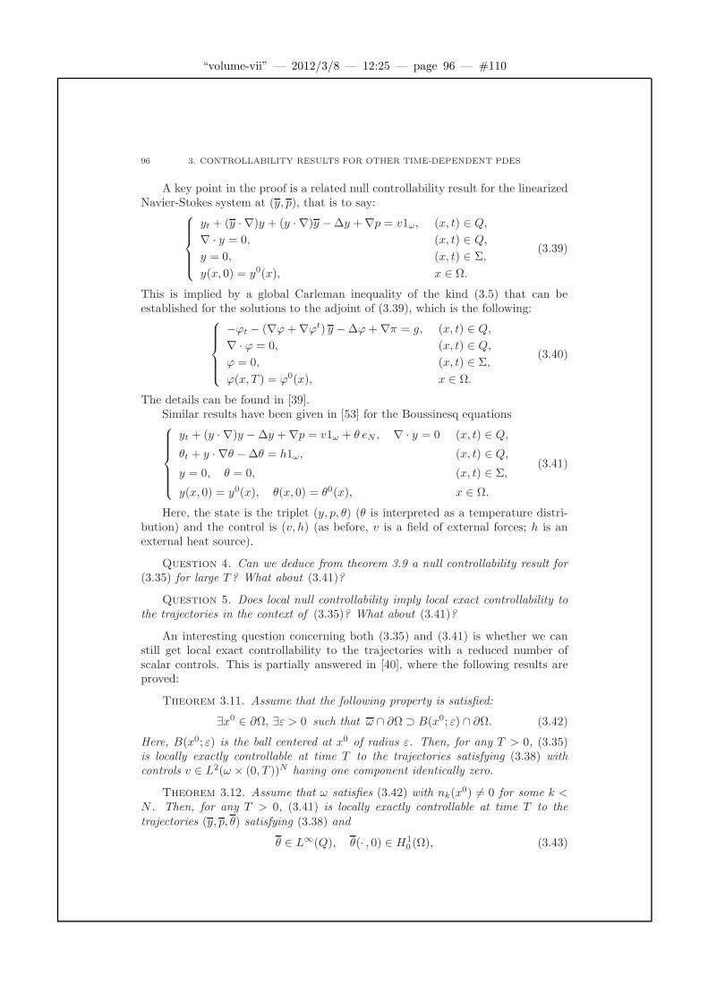
“volume-vii” — 2012/3/8 — 12:25 — page 96 — #110


A key point in the proof is a related null controllability result for the linearizedNavier-Stokes system at (y, p), that is to say:

yt + (y · ∇)y + (y · ∇)y −∆y +∇p = v1ω, (x, t) ∈ Q,

∇ · y = 0, (x, t) ∈ Q,

y = 0, (x, t) ∈ Σ,

y(x, 0) = y0(x), x ∈ Ω.

(3.39)

This is implied by a global Carleman inequality of the kind (3.5) that can beestablished for the solutions to the adjoint of (3.39), which is the following:

−ϕt − (∇ϕ+∇ϕt) y −∆ϕ+∇π = g, (x, t) ∈ Q,

∇ · ϕ = 0, (x, t) ∈ Q,

ϕ = 0, (x, t) ∈ Σ,

ϕ(x, T ) = ϕ0(x), x ∈ Ω.

(3.40)

The details can be found in [39].Similar results have been given in [53] for the Boussinesq equations

yt + (y · ∇)y −∆y +∇p = v1ω + θ eN , ∇ · y = 0 (x, t) ∈ Q,

θt + y · ∇θ −∆θ = h1ω, (x, t) ∈ Q,

y = 0, θ = 0, (x, t) ∈ Σ,

y(x, 0) = y0(x), θ(x, 0) = θ0(x), x ∈ Ω.

(3.41)

Here, the state is the triplet (y, p, θ) (θ is interpreted as a temperature distri-bution) and the control is (v, h) (as before, v is a field of external forces; h is anexternal heat source).

Question 4. Can we deduce from theorem 3.9 a null controllability result for(3.35) for large T? What about (3.41)?

Question 5. Does local null controllability imply local exact controllability tothe trajectories in the context of (3.35)? What about (3.41)?

An interesting question concerning both (3.35) and (3.41) is whether we canstill get local exact controllability to the trajectories with a reduced number ofscalar controls. This is partially answered in [40], where the following results areproved:

Theorem 3.11. Assume that the following property is satisfied:

∃x0 ∈ ∂Ω, ∃ε > 0 such that ω ∩ ∂Ω ⊃ B(x0; ε) ∩ ∂Ω. (3.42)

Here, B(x0; ε) is the ball centered at x0 of radius ε. Then, for any T > 0, (3.35)is locally exactly controllable at time T to the trajectories satisfying (3.38) withcontrols v ∈ L2(ω × (0, T ))N having one component identically zero.

Theorem 3.12. Assume that ω satisfies (3.42) with nk(x0) 6= 0 for some k <

N . Then, for any T > 0, (3.41) is locally exactly controllable at time T to thetrajectories (y, p, θ) satisfying (3.38) and

θ ∈ L∞(Q), θ(· , 0) ∈ H10 (Ω), (3.43)

“volume-vii” — 2012/3/8 — 12:25 — page 97 — #111

6. SOME OTHER NONLINEAR SYSTEMS FROM MECHANICS 97

with controls v ∈ L2(ω × (0, T ))N and h ∈ L2(ω × (0, T )) such that vk ≡ vN ≡ 0.In particular, if N = 2, we have local exact controllability to these trajectories withcontrols v ≡ 0 and h ∈ L2(ω × (0, T )).

The proofs of theorems 3.11 and 3.12 are similar to the proof of theorem 3.9.We have again to rewrite the controllability property as a nonlinear equation in aHilbert space. Then, we have to check that the hypotheses of Liusternik’s theoremare fulfilled.

Again, a crucial point is to prove the null controllability of certain linearizedsystems, this time with modified controls. For instance, when dealing with (3.35),the task is reduced to prove that, for some appropriate weights ρ, ρ0 and someK > 0, the solutions to (3.40) satisfy the following Carleman-like estimates:∫∫

Ω×(0,T )

ρ−2|ϕ|2 dx dt ≤ K

∫∫

ω×(0,T )

ρ−20 (|ϕ1|2 + |ϕ2|2) dx dt ∀ϕ0 ∈ H. (3.44)

This inequality can be proved using the assumption (3.42) and the incompress-ibility identity ∇ · ϕ = 0; see [40].

6. Some other nonlinear systems from mechanics

The previous arguments can be applied to other similar partial differentialsystems arising in mechanics. For instance, this is done in [38] in the context ofmicropolar fluids.

To fix ideas, let us assume that N = 3. The behavior of a micropolar three-dimensional fluid is governed by a system which has the form

yt −∆y + (y · ∇)y +∇p = ∇× w + v1ω, ∇ · y = 0, (x, t) ∈ Q,

wt + (y · ∇)w −∆w −∇(∇ · w) = ∇× y + u1ω, (x, t) ∈ Q,

y = 0, w = 0 (x, t) ∈ Σ,

y(x, 0) = y0(x), w(x, 0) = w0(x) x ∈ Ω.

(3.45)

Here, the state is (y, p, w) and the control is (v, u). As usual, y and p stand forthe velocity field and pressure and w is the microscopic velocity of rotation of thefluid particles.

The following result holds:

Theorem 3.13. Let (y, p, w) be such that

y, w ∈ L∞(Q) ∩ L2(0, T ;H2(Ω)), yt, wt ∈ L2(Q) (3.46)

and

yt −∆y + (y · ∇)y +∇p = ∇× w, ∇ · y = 0, (x, t) ∈ Q,

wt + (y · ∇)w −∆w −∇(∇ · w) = ∇× y, (x, t) ∈ Q,

y = 0, w = 0 (x, t) ∈ Σ.

(3.47)

Then, for each T > 0, (3.45) is locally exactly controllable to (y, p, w) at time T . Inother words, there exists δ > 0 such that, for any initial data (y0, w0) ∈ (H2(Ω) ∩V )×H1

0 (Ω) satisfying

‖(y0, w0)− (y(· , 0), w(· , 0))‖H2×H10≤ δ, (3.48)

“volume-vii” — 2012/3/8 — 12:25 — page 98 — #112


there exist L2 controls u and v and associated solutions (y, p, w) satisfying

y(x, T ) = y(x, T ), w(x, T ) = w(x, T ) in Ω. (3.49)

Notice that this case involves a nontrivial difficulty. Indeed, w is a non-scalarvariable and the equations satisfied by its components wi are coupled throughthe second-order terms ∂i(∇ · w). This is a serious inconvenient. An appropriatestrategy has to be applied in order to deduce the required Carleman estimates.

Let us also mention [7, 61, 62], where the controllability of the MHD and otherrelated equations has been analyzed.

For all these systems, the proof of the controllability can be achieved arguingas in the first part of the proof of theorem 3.9. This is the general structure of theargument:

• First, rewrite the original controllability problem as a nonlinear equationin a space of admissible “state-control” variables.

• Then, prove an appropriate global Carleman inequality and a regularityresult and deduce that the linearized equation possesses at least one solu-tion. This provides a controllability result for a related linear problem.

• Finally, check that the hypotheses of a suitable implicit function theoremare satisfied and deduce a local result.

Remark 3.14. Recall that an alternative strategy was introduced in [109] inthe context of the semilinear wave equation:

• First, consider a linearized similar problem and rewrite the original con-trollability problem in terms of a fixed point equation.

• Then, prove a global Carleman inequality and deduce an observability es-timate for the adjoint system and a controllability result for the linearizedproblem.

• Finally, prove appropriate estimates for the control and the state (thisusually needs some kind of smallness of the data), prove an appropriatecompactness property of the state and deduce that there exists at leastone fixed point.

This method has been used in [30] and [44] in the context of semilinear heatequations and in [52] to prove a result similar to theorem 3.9.

Remark 3.15. Observe that all these results are positive, in the sense that theyprovide local controllability properties. At present, no negative result is known tohold for these nonlinear systems (except for the already considered one-dimensionalBurgers equation).

To end this Section, let us mention two systems from fluid mechanics, appar-ently not much more complex than (3.35), for which local controllability to thetrajectories is an open question.

The first system is the following:

yt + (y · ∇)y −∇ · (ν(|Dy|)Dy) +∇p = v1ω , (x, t) ∈ Q,

∇ · y = 0, (x, t) ∈ Q,

y = 0, (x, t) ∈ Σ,

y(x, 0) = y0(x), x ∈ Ω.

(3.50)

“volume-vii” — 2012/3/8 — 12:25 — page 99 — #113

6. SOME OTHER NONLINEAR SYSTEMS FROM MECHANICS 99

Here, Dy = 12 (∇y +∇yt) and ν : R+ 7→ R+ is a regular function (for example, we

can take ν(s) ≡ a + bsr−1 for some a, b > 0 and some r > 1). This models thebehavior of a quasi-Newtonian fluid; for a mathematical analysis, see [11, 83].

In view of the new nonlinear diffusion term ∇·(ν(|Dy|)Dy), the control proper-ties of (3.51) are much more difficult to analyze than for (3.35). In particular, it isunknown whether the local approximate and the local null controllability propertieshold for (3.50).

For the second system, we suppose that N = 2. It reads:

θt + (y · ∇)θ −∆θ = v1ω , (x, t) ∈ Q,

y = ∇×((−∆)−aθ

), (x, t) ∈ Q,

θ = 0, (x, t) ∈ Σ,

θ(x, 0) = θ0(x), x ∈ Ω,

(3.51)

where a ∈ [1/2, 1]. We are now modelling the behavior of a quasi-geostrophic fluid.The state variables θ and y may be viewed as a generalized vorticity and velocityfield, respectively (notice that, for a = 1, we find again the Navier-Stokes systemwritten in terms of y and ∇× y; see for instance [92]).

It is possible to prove a local null controllability result for (3.51). However, toour knowledge, the local approximate controllability and the local exact controlla-bility to the trajectories are open problems.

“volume-vii” — 2012/3/8 — 12:25 — page 100 — #114

“volume-vii” — 2012/3/8 — 12:25 — page 101 — #115

Bibliography

[1] R.A. Adams, Sobolev Spaces, Academic Press, New York 1975.[2] G. Alessandrini and L. Escauriaza, Null-controllability of one-dimensional par-

abolic equations, ESAIM Control Optim. Calc. Var. 14, no. 2, 2007, 284–293.[3] S. Alinhac, Non unicite du probleme de Cauchy, Annals of Mathematics, 117

(1983), 77–108.[4] F. Ammar-Khodja, A, Benabdallah, C. Dupaix and M. Gonzalez-Burgos, A

Kalman rank condition for the localized distributed controllability of class oflinear parabolic systems, J. Evol. Equ. 9 (2009), no. 2, 267–291.

[5] S. Anita and D. Tataru, Null controllability for the dissipative semilinear heatequation, Appl. Math. Optim. 46, 2002, 97–105.

[6] L. Arnold, Stochastic differential equations: theory and applications, Wiley-Interscience [John Wiley & Sons], New York-London-Sydney, 1974.

[7] V. Barbu V, T. Havarneanu, C. Popa and S.S. Sritharan SS, Exact controlla-bility for the magnetohydrodynamic equations, Comm. Pure Appl. Math. 56,2003, 732–783.

[8] V. Barbu, A. Rascanu and G. Tesitore, Carleman estimates and controllabilityof linear stochastic heat equations, Appl. Math. Optim. 47 (2003), no. 2, 97–120.

[9] C. Bardos, G. Lebeau and J. Rauch, Sharp sufficient conditions for the obser-vation, control and stabilization of waves from the boundary, SIAM J. Cont.Optim., 30 (1992), 1024–1065.

[10] J.A. Bello, E. Fernandez-Cara, J. Lemoine and J. Simon, The differentiabilityof the drag with respect to the variations of a Lipschitz domain in a Navier-Stokes flow, SIAM J. Control Optimiz., Vol. 35, No. 2, pp. 626–640, 1997.

[11] H. Bellout, F. Bloom and J. Necas, Young measure-valued solutions for non-Newtonian incompressible fluids, Comm. PDE 19, no. 11–12, 1994, 1763–1803.

[12] A. Benabdallah, Y. Dermenjian, Yves and J. Le Rousseau, Carleman estimatesfor the one-dimensional heat equation with a discontinuous coefficient and ap-plications to controllability and an inverse problem, J. Math. Anal. Appl. 336(2007), no. 2, 865–887.

[13] A. Benabdallah, Y. Dermenjian, Yves and J. Le Rousseau, to appear.[14] J.F. Bonnans and E. Casas, Optimal control of semilinear multistate systems

with state constraints, SIAM J. Control Optimiz. 27 (1989), No. 2, 446–455.[15] N. Burq, Controle de l’equation des ondes dans des ouverts peu reguliers,

Asymptotic Analysis, 14 (1997), 157–191.[16] E. Casas, Boundary control of semilinear elliptic equations with pointwise state

constraints, SIAM J. Control Optimiz. 31 (1993), No. 4, 996–1006.

101

“volume-vii” — 2012/3/8 — 12:25 — page 102 — #116

102 BIBLIOGRAPHY

[17] E. Casas and L.A. Fernandez, Optimal control of semilinear elliptic equationswith pointwise constraints on the gradient of the state, Appl. Math. Optim. 27(1993), No. 1, 35–56.

[18] T. Cazenave, On the propagation of confined waves along the geodesics,J. Math. Anal. Appl., 146 (1990), 591–603.

[19] D. Chae, O.Yu. Imanuvilov and S.M. Kim, Exact controllability for semilin-ear parabolic equations with Neumann boundary conditions, J. Dynamical andControl Systems 2 (1996), 449–483.

[20] M. Chapouly, Global controllability of nonviscous and viscous Burgers-typeequations, SIAM J. Control Optim. 48 (2009), no. 3, 1567–1599.

[21] D. Chenais, On the existence of a solution in a domain identification problem,J. Math. Anal. Appl. 52 (2) (1975), 430–445.

[22] J.-M. Coron, On the controllability of the 2-D incompressible Navier-Stokesequations with the Navier slip boundary conditions, ESAIM Control Optim.Calc. Var. 1, (1995/96), 35–75.

[23] J.-M. Coron, Control and nonlinearity, Control and nonlinearity, Mathemat-ical Surveys and Monographs, 136. American Mathematical Society, Provi-dence, RI, 2007.

[24] G. DaPrato and J. Zabczyk, Stochastic Equations in Infinite Dimensions,Cambridge University Press, Cambridge 1992.

[25] C. Dellacherie, Analytical Sets, Capacities and Haussdorff Measures, LecturesNotes in Mathematics, No. 180, Springer-Verlag, Berlin 1972.

[26] A. Doubova, E. Fernandez-Cara, M. Gonzalez-Burgos and E. Zuazua, On thecontrollability of parabolic systems with a nonlinear term involving the stateand the gradient, SIAM J. Control Optim. 41 (2002), no. 3, 798–819.

[27] A. Doubova, A. Osses and J.-P. Puel, Exact controllability to trajectoriesfor semilinear heat equations with discontinuous diffusion coefficients, ESAIMControl Optim. Calc. Var. 8 (2002), 621–661.

[28] R. Echevarrıa, A. Doubova, E. Fernandez-Cara and I. Gayte, Control de EDPsorientado a la terapia de un tumor cerebral, Communication to CEDYA 2007,Sevilla, 2007.

[29] C. Fabre, Uniqueness results for Stokes equations and their consequences inlinear and nonlinear control problems, ESAIM Control Optim. Calc. Var. 1,(1995/96), 267–302.

[30] C. Fabre, J.-P. Puel and E. Zuazua, Approximate controllability of the semi-linear heat equation, Proc. Royal Soc. Edinburgh A 125 (1995), 31–61.

[31] C. Fabre, J.P. Puel and E. Zuazua, Controlabilite approchee de l’equation dela chaleur lineaire avec des controles de norme L∞ minimale, C.R. Acad. Sci.Paris, 316 (1993), 679–684.

[32] H.O. Fattorini, Infinite Dimensional Optimization and Control Theory, Ency-clopedia of Mathematics and its Applications 62, Cambridge University Press,1999.

[33] L.A. Fernandez and E. Zuazua, Approximate controllability for the semilinearheat equation involving gradient terms, J. Optim. Theory Appl. 101 (1999),no. 2, 307–328.

[34] E. Fernandez-Cara, M.J. Garrido-Atienza and J. Real, On the approximatecontrollability of a stochastic parabolic equation with a multiplicative noise,

“volume-vii” — 2012/3/8 — 12:25 — page 103 — #117

BIBLIOGRAPHY 103

C.R. Acad. Sci. Paris 328 (1999), 675–680.[35] E. Fernandez-Cara, M. Gonzalez-Burgos and L. De Teresa, Null-exact control-

lability of a semilinear cascade system of parabolic-hyperbolic equations, Comm.Pure Applied Anal. 5 (2008), no. 3, 639–658.

[36] E. Fernandez-Cara and S.Guerrero, Global Carleman inequalities for parabolicsystems and applications to controllability, SIAM J. Control Optim. 45 (2006),no. 4, 1399–1446.

[37] E. Fernandez-Cara and S. Guerrero, Null controllability of the Burgers systemwith distributed controls, Systems Control Lett. 56 (2007), no. 5, 366–372.

[38] E. Fernandez-Cara and S. Guerrero, Local exact controllability of micropolarfluids, J. Math. Fluid. Mech. 8 (2006), 1–35.

[39] E. Fernandez-Cara, S. Guerrero, O.Yu. Imanuvilov and J.-P. Puel, Local exactcontrollability to the trajectories of the Navier-Stokes equations, J. Math. PuresAppl. 83 (2004), no. 12, 1501–1542.

[40] E. Fernandez-Cara, S. Guerrero, O.Yu. Imanuvilov and J.-P. Puel, Some con-trollability results for the N -dimensional Navier-Stokes and Boussinesq sys-tems with N−1 scalar controls, SIAM J. Control and Optim. 45 (2006), no. 1,146–173.

[41] E. Fernandez-Cara. J.D. Martın and J. Real, On the approximate controllabilityof stochastic Stokes systems, Stoch. Anal. Appl. 17 (1999), no. 4, 563–577.

[42] E. Fernandez-Cara and J. Real, Remarks on the controllability of some stochas-tic partial differential equations, in “Control and Estimation of Distributed Pa-rameter Systems”, p. 141–151, International Series of Numerical Mathematics,Birkhauser Verlag, Basel 1998.

[43] E. Fernandez-Cara and E. Zuazua, The cost of approximate controllability forheat equations: The linear case, Advances Diff. Eqs. 5 (2000), no. (4–6), 465–514.

[44] E. Fernandez-Cara and E. Zuazua, Null and approximate controllability forweakly blowing up semilinear heat equations, Ann. Inst. H. Poincare Anal. NonLineaire 17 (2000), no. 5, 583–616.

[45] A.V. Fursikov, Exact boundary zero-controllability of three-dimensional Navier-Stokes equations, J. Dynam. Control Systems 1 (1995), no. 3, 325–350.

[46] A.V. Fursikov and O.Yu. Imanuvilov, On exact boundary zero-controllabilityof two-dimensional Navier-Stokes equations, Acta Applicandae Mathematicae37 (1994), 67–76.

[47] A.V. Fursikov and O.Yu. Imanuvilov, Controllability of evolution equations,Lecture Notes Series # 34, Research Institute of Mathematics, Global AnalysisResearch Center, Seoul National University, 1996.

[48] A.V. Fursikov and O.Yu. Imanuvilov, Local exact controllability of the Boussi-nesq equation, SIAM J. Cont. Opt. 36 (1998), no. 2, 391–421.

[49] A.V. Fursikov and O. Yu. Imanuvilov, Exact controllability of the Navier-Stokesand Boussinesq equations (Russian), Uspekhi Mat. Nauk 54 (1999), no. 3(327),93–146; translation in Russian Math. Surveys 54 (1999), no. 3, 565–618.

[50] P. Gerard, Microlocal defect measures, Comm. P.D.E. 16 (1991), 1761–1794.[51] V. Girault and Ph.-A. Raviart, Finite element methods for Navier-Stokes equa-

tions. Theory and algorithms, Springer-Verlag, Berlin, 1986.

“volume-vii” — 2012/3/8 — 12:25 — page 104 — #118

104 BIBLIOGRAPHY

[52] M. Gonzalez-Burgos, S. Guerrero and J.-P. Puel, Local exact controllability tothe trajectories of the Boussinesq system via a fictitious control on the diver-gence equation, Commun. Pure Appl. Anal. 8 (2009), no. 1, 311–333.

[53] S. Guerrero, Local exact controllability to the trajectories of the Boussinesqsystem, Annales IHP, Anal. non lineaire 23 (2006), 29–61.

[54] S. Guerrero and O. Yu. Imanuvilov, Remarks on global controllability for theBurgers equation with two control forces, Ann. Inst. H. Poincare Anal. NonLineaire 24 (2007), no. 6, 897–906.

[55] R. Glowinski, Ensuring well-posedness by analogy; Stokes problem and bound-ary control for the wave equation, J. Compt. Physics 103 (1992), no. 2, 189–221.

[56] R. Glowinski, C.H. Li and J.-L. Lions, A numerical approach to the exactboundary controllability of the wave equation (I). Dirichlet controls: Descrip-tion of the numerical methods, Japan J. Appl. Math. 7 (1990), 1–76.

[57] R. Glowinski and J.-L. Lions, Exact and approximate controllability for dis-tributed parameter systems, Acta Numerica 1994, p. 269–378.

[58] R. Glowinski, J.-L. Lions and J. He, Exact and approximate controllability fordistributed parameter systems. A numerical approach, Encyclopedia of Math-ematics and its Applications, 117. Cambridge University Press, Cambridge,2008.

[59] M.D. Gunzburger, Perspectives in flow control and optimization, Advances indesign and control, 5. SIAM, Philadelphia, 2003.

[60] J. Haslinger and P. Neittaanmaki, Finite Element Approximation for OptimalShape Design, John Wiley and Sons, Chichester, 1988.

[61] T. Havarneanu, C. Popa and S.S. Sritharan, Exact internal controllability forthe magnetohydrodynamic equations in multi-connected domains, Adv. Differ.Equations 11 (2006), no. 8, 893–929.

[62] T. Havarneanu, C. Popa and S.S. Sritharan, Exact internal controllability forthe two-dimensional magnetohydrodynamic equations, SIAM J. Control Op-tim. 46 (2007), no. 5, 1802–1830.

[63] L.F. Ho, Observabilite frontiere de l’equation des ondes, C.R. Acad. Sci. Paris302 (1986), 443–446.

[64] O.Yu. Imanuvilov, Boundary controllability of parabolic equations, RussianAcad. Sci. Sb. Math. 186 (1995), 109–132 (in Russian).

[65] O. Yu. Imanuvilov, Remarks on exact controllability for the Navier-Stokesequations, ESAIM Control Optim. Calc. Var. 6 (2001), 39–72.

[66] O.Yu. Imanuvilov and M. Yamamoto, Carleman inequalities for parabolic equa-tions in Sobolev spaces of negative order and exact controllability for semilinearparabolic equations, Publ. Res. Inst. Math. Sci. 39 (2003), no. 2, 227–274.

[67] R. Kohn and G. Strang, Optimal design and relaxation of variational problems,I, II and III, Comm. Pure Appl. Math. 34 (1986), 113–137, 139–182 and 353–377.

[68] I. Lasiecka and R. Triggiani, Exact controllability of semilinear abstract systemswith application to waves and plates boundary control problems, Appl. Math.Optim. 23 (1991), no. 2, 109–154.

[69] G. Lebeau, Controle analytique I: estimations a priori, Duke Math. J. 68

(1992), no. 1, 1–30.

“volume-vii” — 2012/3/8 — 12:25 — page 105 — #119

BIBLIOGRAPHY 105

[70] G. Lebeau and L. Robbiano, Controle exact de l’equation de la chaleur,Comm. P.D.E. 20 (1995), 335–356.

[71] E.B. Lee and L. Markus, Foundations of Optimal Control Theory, The SIAMSeries in Applied Mathematics, John Wiley & Sons, New York 1967.

[72] S. Lenhart and J.T. Workman Optimal control applied to biological models,Chapman & Hall / CRC, 2007.

[73] J. Le Rousseau and L. Robbiano, Carleman estimate for elliptic operators withcoefficients with jumps at an interface in arbitrary dimension and applicationto the null controllability of linear parabolic equations, Arch. Ration. Mech.Anal. 195 (2010), no. 3, 953–990.

[74] G. Leugering and E. Zuazua, On exact controllability of generic trees, in“Controle de Systemes Gouvernes par des Equations aux Derivees Partielles”,ESAIM Proceedings, Vol. 8, F. Conrad and M. Tucsnak eds., pp. 95–105.

[75] X. Li and J. Yong, Optimal Control Theory for Infinite Dimensional Systems,Birkhauser, Boston, 1995.

[76] J.-L. Lions, Controle Optimale des Systemes Gouvernes par des Equations auxDerivees Partielles, Dunod, Gauthiers-Villars, Paris, 1968.

[77] J.-L. Lions, Exact controllability, stabilizability and perturbations for dis-tributed systems, SIAM Review 30 (1988), 1–68.

[78] J.-L. Lions, Controlabilite Exacte, Stabilisation et Perturbations de SystemesDistribues, Tomes 1 & 2. Masson, RMA 8 & 9, Paris 1988.

[79] J.-L. Lions, Remarques sur la controlabilite approchee, in Jornadas Hispano-Francesas sobre Control de Sistemas Distribuidos, University of Malaga, Spain,1991, pp. 77–87.

[80] J.-L. Lions, Remarks on approximate controllability, J. Anal. Math. 59 (1992),103–116.

[81] J.-L. Lions and B. Malgrange, Sur l’unicite retrograde dans les problemesmixtes paraboliques, Math. Scan. 8 (1960), 277–286.

[82] K.A. Lurie, Applied Optimal Control Theory of Distributed Systems, PlenumPress, New York, 1993.

[83] J. Malek, J. Necas, M. Rokyta, M. Ruzicka M, Weak and measure-valued so-lutions to evolutionary PDEs, Applied Mathematics and Mathematical Com-putation, 13, Chapman & Hall, London, 1996.

[84] F. Murat, H-convergence, Lectures at the University of Alger, Alger, 1978.[85] F. Murat, H-convergence, in “Topics in the Mathematical Modelling of Com-

posite Materials”, A. Cherkaev and R. Kohn eds., Birkhauser, Boston, 1997.[86] F. Murat and J. Simon, Quelques resultats sur le controle par un domaine

geometrique, Rapport du L.A. 189 No. 74003, Universite Paris VI, 1974.[87] F. Murat and J. Simon, Sur le controle par un domaine geometrique, Rapport

du L.A. 189 No. 76015, Universite Paris VI, 1976.[88] F. Murat and L. Tartar, On the control of coefficients in partial differential

equations, in “Topics in the Mathematical Modelling of Composite Materials”,A. Cherkaev and R. Kohn eds., Birkhauser, Boston 1997.

[89] A. Osses, A rotated multiplier applied to the controllability of waves, elasticity,and tangential Stokes control, SIAM J. Control Optim. 40 (2001), no. 3, 777–800

[90] E. Pardoux, PhD Thesis, Universite Paris XI (France), 1975.

“volume-vii” — 2012/3/8 — 12:25 — page 106 — #120

106 BIBLIOGRAPHY

[91] E. Pardoux, Integrales stochastiques hilbertiennes, Cahiers de Mathematiquesde la Decision No. 7617, Universite Paris IX,1976.

[92] J. Pedlosky, Geophysical fluid dynamics, Second edition, Springer, New York,1987.

[93] P. Pedregal, Optimization, relaxation and Young measures, Bull. A.M.S. 36(1999), no. 1, 27–58.

[94] O. Pironneau, On optimum design in fluid mechanics, J. Fluid Mech. 64

(1974), 97–110.[95] O. Pironneau, PhD Thesis, Universite Pierre & Marie Curie (Paris VI; France),

1976.[96] O. Pironneau, Optimal Shape Design for Elliptic Systems, Springer-Verlag,

New-York, 1984.[97] J.-P. Puel, Global Carleman inequalities for the wave equations and applica-

tions to controllability and inverse problems, in “Control of Solids and Struc-tures: Mathematical Modelling and Engineering Applications”, Udine (Italy),June 2004.

[98] L. Robbiano and C. Zuily, Uniqueness in the Cauchy problem for operatorswith partially holomorphic coefficients, Invent. Math. 131 (1998), 493–539.

[99] D.L. Russell, Controllability and stabilizability theory for linear partial differ-ential equations. Recent progress and open questions, SIAM Review 20 (1978),639–739.

[100] D.L. Russell, A unified boundary controllability theory for hyperbolic and para-bolic partial differential equations, Studies in Appl. Math., 52 (1973), 189–221.

[101] J. Simon, Second variation in domain optimization problems, in “Controland Estimation of Distributed Parameter Systems”, F. Kappel, K. Kunishand W. Schappacher eds., Int. Series of Numer. Math., No. 91, p. 361–378,Birkhauser, 1989.

[102] J. Sokolowski and J.-P. Zolesio, Introduction to Shape Optimization, Springer-Verlag, Berlin, 1992.

[103] K. R. Swanson, E. C. Alvord Jr. and J. D. Murray, A quantitative model fordifferential motility of gliomas in grey and white matter, Cell Prolif. 33 (2000),317–329.

[104] K. R. Swanson, E. C. Alvord Jr. and J. D. Murray, Quantifying the efficacy ofchemotherapy of brain tumors (gliomas) with homogeneous and heterogeneousdrug delivery, Acta Biotheoretica 50 (2002), no. 4, 223–237.

[105] D. Tataru, Unique continuation for solutions to PDE’s: between Hormander’stheorem and Holmgren’s theorem, Comm. PDE 20 (1995), no. 6–7, 855–884.

[106] L. Tartar, Problemes de controle des coefficients dans des equations auxderivees partielles, in “Control theory, numerical methods and computer sys-tems modelling”, A. Bensoussan and J.L. Lions eds., Lecture Notes in Eco-nomics and Mathematical Systems No. 107, Springer-Verlag, Berlin, 1975.

[107] X. Zhang, Explicit observability estimate for the wave equation with potentialand its application, R. Soc. Lond. Proc. Ser. A, Math. Phys. Eng. Sci. 456(2000), no. 1997, 1101–1115.

[108] X. Zhang, A unified controllability/observability theory for some stochasticand deterministic partial dfferential equations, Proc. ICM, Hyderabad, India,2010.

“volume-vii” — 2012/3/8 — 12:25 — page 107 — #121

BIBLIOGRAPHY 107

[109] E. Zuazua E, Exact boundary controllability for the semilinear wave equation,in “Nonlinear Partial Differential Equations and their Applications”, Vol. X(p. 357–391), H. Brezis and J.L. Lions eds., Pitman, New York, 1991.

[110] E. Zuazua, Finite dimensional null controllability for the semilinear heat equa-tion, J. Math. Pures Appl. 76 (1997), 570–594.

[111] E. Zuazua Controllability and observability of partial differential equations:some results and open problems, Handbook of differential equations: evolution-ary equations, Vol. III, 527–621, Handb. Differ. Equ., Elsevier/North-Holland,Amsterdam, 2007.

“volume-vii” — 2012/3/8 — 12:25 — page 108 — #122

“volume-vii” — 2012/3/8 — 12:25 — page 109 — #123

Part 4

Fluid-structure interaction for

shear-dependent non-Newtonian

fluids

Anna Hundertmark-Zauskova,

Maria Lukacova-Medvid’ova, Gabriela Rusnakova

“volume-vii” — 2012/3/8 — 12:25 — page 110 — #124

2000 Mathematics Subject Classification. Primary 65M60, 35Q30, 74F10, 65N30,76D05, 35M99

Key words and phrases. non-Newtonian fluids, fluid-structure interaction,shear-thinning flow, hemodynamical wall parameters, stenosis, kinematical

splitting, numerical stability, weak solution

Abstract. We present our recent results on mathematical modelling andnumerical simulation of non-Newtonian flows in compliant two-dimensionaldomains having applications in hemodynamics. Two models of the shear-thinning non-Newtonian fluids, the power law Carreau model and the loga-rithmic Yeleswarapu model, will be considered. For the structural model thegeneralized string equation for radially symmetric tubes will be generalized tostenosed vessels and vessel bifurcations.

The arbitrary Lagrangian-Eulerian approach is used in order to take intoaccount moving computational domains. To represent the fluid-structure in-teraction we use two different methods: the global iterative approach andthe kinematical splitting. We will show that the latter method is more effi-cient and stable without any additional subiterations. The analytical resultfor the existence of a weak solution for the shear-thickening power-law fluidis based on the global iteration with respect to the domain deformation, en-ergy estimates, compactness arguments using the semi-continuity in time andthe theory of monotone operators. The numerical part of paper contains sev-eral experiments for the Carreau and the Yeleswarapu model, comparisons ofthe non-Newtonian and Newtonian models and the results for hemodynamicalwall parameters; the wall shear stress and the oscillatory shear index. Nu-merical experiments confirm higher order accuracy and the reliability of newfluid-structure interaction methods.

Acknowledgement. This research has been supported by the EuropeanUnion’s 6th Framework Programme DEASE under the No. MEST-CT-2005-021122, the German Science Foundation (DFG) project ZA 613/1-1 as wellas by the Necas Centrum for Mathematical Modelling LC06052 (financed byMSMT). The third author has been partially supported by the Center forComputational Sciences in Mainz and the German Academic Exchange Ser-vice DAAD. The authors gratefully acknowledge these supports.

“volume-vii” — 2012/3/8 — 12:25 — page 111 — #125

Contents

Chapter 1. Fluid-structure interaction methods 1131. Introduction 1132. Mathematical model for shear-dependent fluids 1143. Generalized string model for the wall deformation 1174. Fluid-structure interaction methods 1214.1. Strong coupling: global iterative method 1214.1.1. Existence of a weak solution to the coupled problem 1234.2. Weak coupling: kinematical splitting algorithm 1264.2.1. Stability analysis 127

Chapter 2. Numerical study 1311. Numerical study 1311.1. Hemodynamical indices 1311.2. Computational geometry and parameter settings 1311.2.1. Boundary conditions 1331.2.2. Parameter settings 1341.3. Discretization methods 1351.3.1. Linearization of the viscous term 1351.3.2. Discretization of structure equation 1361.4. Numerical experiments 1381.4.1. Numerical experiments for model data 1381.4.2. Numerical experiments for physiological data 1411.4.3. Iliac artery and carotid bifurcation 1431.5. Convergence study 1492. Concluding remarks 153

Bibliography 155

111

“volume-vii” — 2012/3/8 — 12:25 — page 112 — #126

“volume-vii” — 2012/3/8 — 12:25 — page 113 — #127

CHAPTER 1

Fluid-structure interaction methods

1. Introduction

In the recent years there is a growing interest in the use of mathematical modelsand numerical methods arising from other fields of computational fluid dynamics inhemodynamics, see, e.g., [6, 8, 18, 19, 21, 27, 31, 36, 37, 39, 40, 41] just to mentionsome of them.

Many numerical methods used for blood flow simulations are based on theNewtonian model using the Navier-Stokes equations. This is efficient and useful,especially if the flow in large arteries is modeled. However, in small vessels ordealing with patients with a cardiovascular disease more complex models for bloodrheology should be considered [31]. In capillaries blood is even not a homogenizedcontinuum and more precise models, for example mixture theories need to be used.But even in the intermediate-size vessels the non-Newtonian behavior of blood hasbeen demonstrated, see, e.g., [2], [43] and the references therein. In fact, blood isa complex mixture showing several non-Newtonian properties, such as the shear-thinning, viscoelasticity [48], [49] the yield stress or the stress relaxation [43].

The aim of this overview paper is to report on our recent results on mathe-matical and numerical modelling of shear-dependent flow in moving vessels. Theapplication to hemodynamics will be pointed out. We will address the significanceof non-Newtonian models for reliable hemodynamical modelling. In particular, wewill show that the rheological properties of fluid have an influence on the wall de-formation as well as on the hemodynamical wall parameters, such as the wall shearstress and oscillatory shear index. Consequently these models yield a more reliableprediction of critical vessel areas, see also our previous results [24, 28, 29].

The paper is organized as follows. In Section 2 we recall the conservationlaws for shear-dependent fluids and present typical models for non-constant bloodviscosity. The generalized string model for the vessel deformation [40] is generalizedto the case of reference radius, which is dependent on longitudinal variable. Thederivation of this model for radially symmetric domains follows in Section 3.

Section 4 is devoted to two strategies to model the coupling between a fluidand a structure. The global iterative method with respect to the domain, presentedin Section 4.1, provides besides the numerical scheme also a strategy to prove theexistence of a weak solution. Mathematical analysis of the well-posedness of acoupled fluid-structure model arising from the blood flow in a compliant vessel is ofgreat interest. In the literature there are already several results for the Newtonianfluid flow in time-dependent domains, see, e.g., [4, 5, 6, 7, 9, 10, 11, 12, 13, 20, 22,23, 33, 47, 51] and others. The well-posedness of non-Newtonian fluids has beenstudied only in the fixed domains, see, e.g., [17, 34, 35, 50]. In these works the

113

“volume-vii” — 2012/3/8 — 12:25 — page 114 — #128

114 1. FLUID-STRUCTURE INTERACTION METHODS

technique of monotone operators and the Lipschitz- or L∞-truncation techniquesare applied in order to control the additional nonlinearities in the diffusion termsarising from the non-Newtonian viscosity. In this overview paper we also presentour recent result on the existence of a weak solution for the shear-thickenning fluidin compliant vessels, cf. [25]. The proof is based on the global iterative methodwith respect to the domain deformation [13, 51], theory of monotone operators aswell as the techniques for moving domains developed in [7, Chambolle, Desjarden,Esteban, Grandmont].

The second fluid-structure interaction approach, that will be presented in Sec-tion 4.2, is the loosely-coupled fluid-structure interaction algorithm based on thekinematical splitting [21]. This is a novel way how to avoid instabilities due tothe added mass effect and the additional stabilization through subiterations. Sub-section 4.2.1 is devoted to stability analysis of the kinematical splitting method.Further details can be found in our recent paper [28].

Results of numerical experiments are described in Section 5. We apply bothfluid-structure interaction methods and compare domain deformations as well thehemodynamical wall indices measuring the danger of atherosclerotic plaque causedby temporal oscillation or low values of the wall shear stress. We use two types ofdata: the model data proposed by Sequeira and Nadau [31] and the physiologicaldata from the iliac artery and the carotid bifurcation measurements. In the hemo-dynamical wall parameters the effects due to the fluid-structure interaction as wellas the blood rheology have been observed. Finally the experimental order of con-vergence for a rigid as well as a moving domain for both fluid-structure interactionmethods will be investigated. In the case of kinematical splitting method secondorder convergence will be confirmed.

2. Mathematical model for shear-dependent fluids

Flow of incompressible fluid is governed by the momentum and the continuityequation

ρ∂u

∂t+ ρ (u · ∇)u− div [2µD(u)] +∇p = f

div u = 0.(2.1)

Here ρ denotes the constant density of fluid, u = (u1, u2) the velocity vector, pthe pressure, D(u) = 1

2 (∇u +∇uT ) the deformation tensor and µ the viscosity ofthe fluid. In the literature various non-Newtonian models for the blood flow canbe found. Here we will consider shear-dependent fluids, in particular the Carreaumodel and the Yeleswarapu-viscosity model [48], see also Fig. 1. For the Car-

reau model the viscosity function depends on the shear rate |D(u)| =√D : D =√

tr(D2) in the following way

µ = µ(D(u)) = µ∞ + (µ0 − µ∞)(1 + |γD(u)|2)q, q =p− 2

2≤ 0, (2.2)

where q, µ0, µ∞, γ are rheological parameters. According to [48] the physiologicalvalues for blood are µ0 = 0.56P, µ∞ = 0.0345P, γ = 3.313, q = −0.322. Notethat in the case q = 0 the model reduces to the linear Newtonian model used in

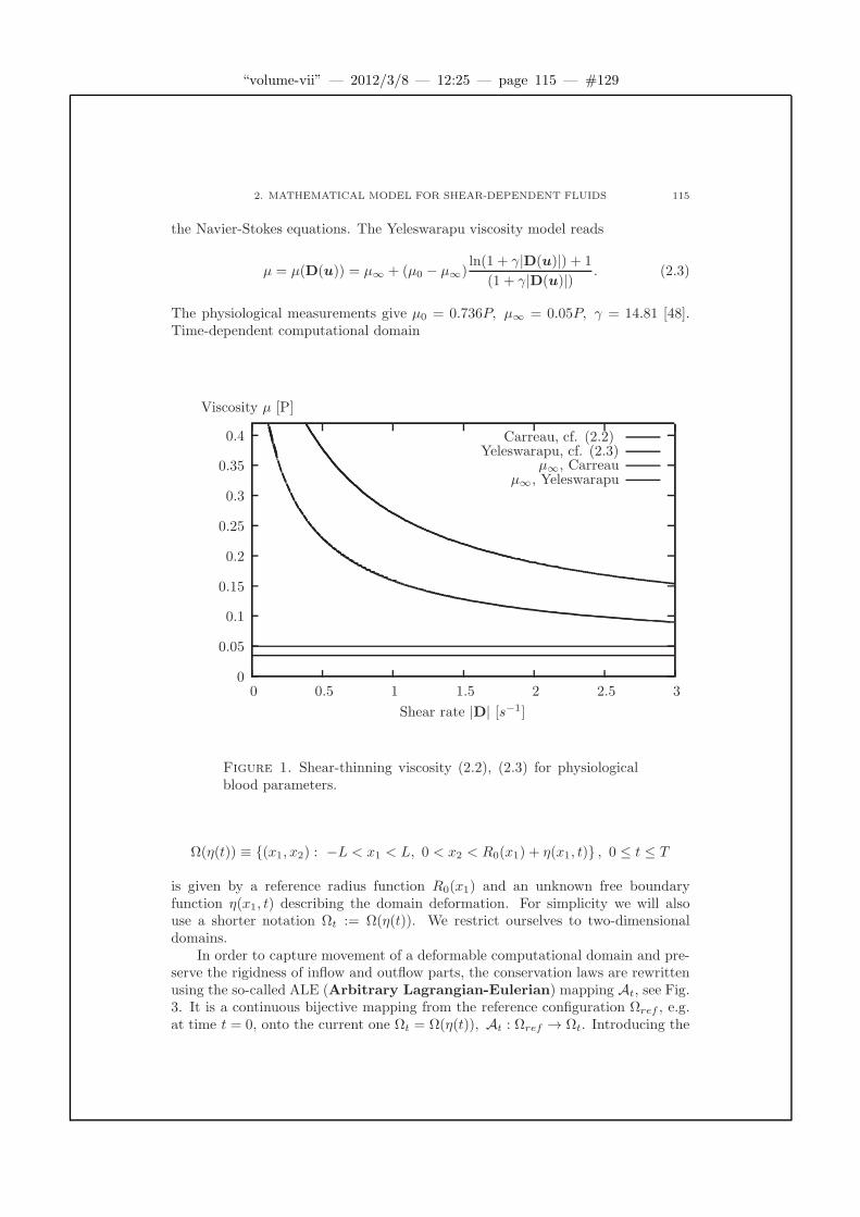
“volume-vii” — 2012/3/8 — 12:25 — page 115 — #129

2. MATHEMATICAL MODEL FOR SHEAR-DEPENDENT FLUIDS 115

the Navier-Stokes equations. The Yeleswarapu viscosity model reads

µ = µ(D(u)) = µ∞ + (µ0 − µ∞)ln(1 + γ|D(u)|) + 1

(1 + γ|D(u)|) . (2.3)

The physiological measurements give µ0 = 0.736P, µ∞ = 0.05P, γ = 14.81 [48].Time-dependent computational domain

0

0.05

0.1

0.15

0.2

0.25

0.3

0.35

0.4

0 0.5 1 1.5 2 2.5 3

Viscosity µ [P]

Shear rate |D| [s−1]

Carreau, cf. (2.2)Yeleswarapu, cf. (2.3)

µ∞, Carreauµ∞, Yeleswarapu

Figure 1. Shear-thinning viscosity (2.2), (2.3) for physiologicalblood parameters.

Ω(η(t)) ≡ (x1, x2) : −L < x1 < L, 0 < x2 < R0(x1) + η(x1, t) , 0 ≤ t ≤ T

is given by a reference radius function R0(x1) and an unknown free boundaryfunction η(x1, t) describing the domain deformation. For simplicity we will alsouse a shorter notation Ωt := Ω(η(t)). We restrict ourselves to two-dimensionaldomains.

In order to capture movement of a deformable computational domain and pre-serve the rigidness of inflow and outflow parts, the conservation laws are rewrittenusing the so-called ALE (Arbitrary Lagrangian-Eulerian) mapping At, see Fig.3. It is a continuous bijective mapping from the reference configuration Ωref , e.g.at time t = 0, onto the current one Ωt = Ω(η(t)), At : Ωref → Ωt. Introducing the

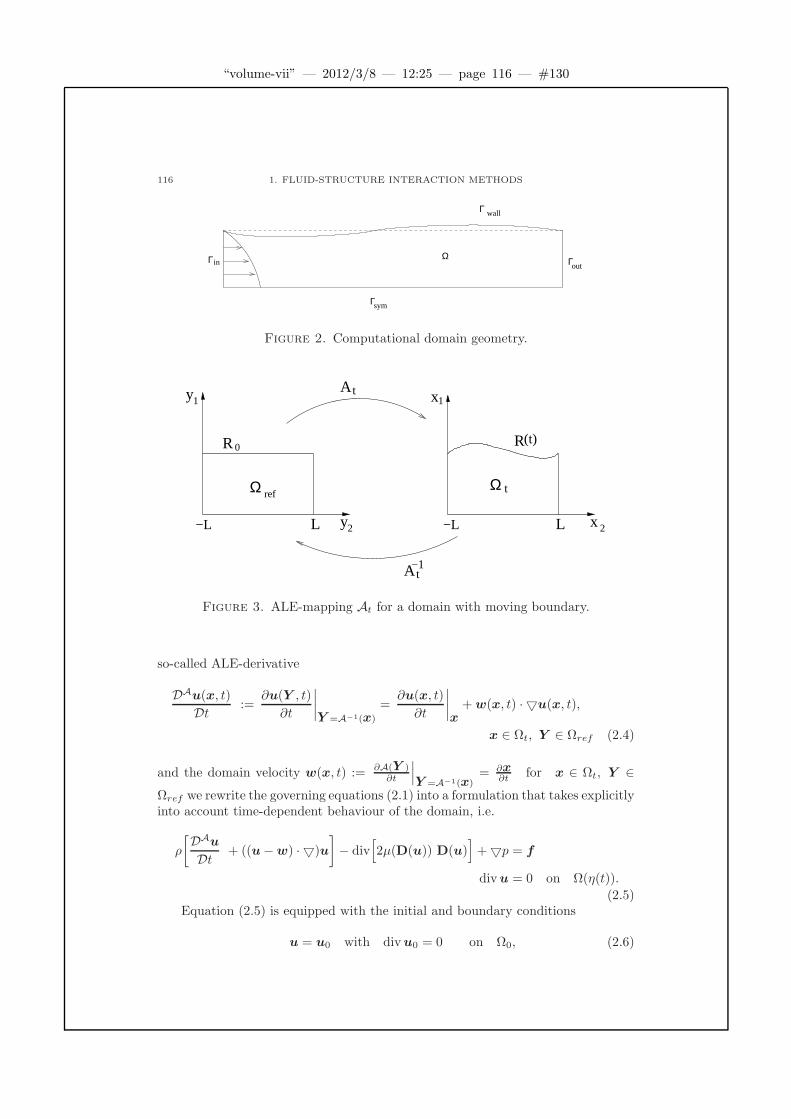
“volume-vii” — 2012/3/8 — 12:25 — page 116 — #130


Γ

Γ

wallΓ

sym

outinΓ Ω

Figure 2. Computational domain geometry.

0R

x 2y

y1

2

A

Ω ref

L L−L −L

(t)

t

tA−1

Ω

x1

t

R

Figure 3. ALE-mapping At for a domain with moving boundary.

so-called ALE-derivative

DAu(x, t)

Dt :=∂u(Y , t)

∂t

∣∣∣∣Y =A−1(x)

=∂u(x, t)

∂t

∣∣∣∣x+w(x, t) · u(x, t),

x ∈ Ωt, Y ∈ Ωref (2.4)

and the domain velocity w(x, t) := ∂A(Y )∂t

∣∣∣Y =A−1(x)

= ∂x∂t for x ∈ Ωt, Y ∈

Ωref we rewrite the governing equations (2.1) into a formulation that takes explicitlyinto account time-dependent behaviour of the domain, i.e.

ρ

[DAu

Dt + ((u−w) · )u

]− div

[2µ(D(u)) D(u)

]+p = f

divu = 0 on Ω(η(t)).

(2.5)Equation (2.5) is equipped with the initial and boundary conditions

u = u0 with divu0 = 0 on Ω0, (2.6)

“volume-vii” — 2012/3/8 — 12:25 — page 117 — #131

3. GENERALIZED STRING MODEL FOR THE WALL DEFORMATION 117

(T(u, p)− 1

2|u|2I

)· n = −Pin I · n, on Γin, t ∈ (0, T ), (2.7)

(T(u, p)− 1

2|u|2I

)· n = −Pout I · n, on Γout, t ∈ (0, T ), (2.8)

∂u1∂x2

= 0, u2 = 0, on Γsym, t ∈ (0, T ). (2.9)

Conditions (2.7) and (2.8) are called the kinematical pressure conditions. Thefluid velocity is coupled with the velocity of wall deformation by the so-called kine-matical coupling condition

u = w :=

(0,∂η

∂t

)T

on Γwall, t ∈ (0, T ). (2.10)

3. Generalized string model for the wall deformation

In order to model biological structure several models have been proposed inliterature. For example, to model flow in a collapsible tubes a two-dimensional thinshell model can be used, see results of Wall et al. [16]. Recently Canic et al. [6]developed a new one-dimensional model for arterial walls, the linearly viscoelas-tic cylindrical Koiter shell model, that is closed and rigorously derived by energyestimates, asymptotic analysis and homogenization techniques. The viscous fluiddissipation imparts long-term viscoelastic memory effects represented by higherorder derivatives.

In the present work we will consider the generalized string model for vessel walldeformation. The original generalized string model, see [40], was valid only forradially symmetric domains with a constant reference radius R0. In order to modelstenotic occlusions we will extend this model and assume that the reference radiusat rest R0 depends on the longitudinal variable.

Let us consider a three-dimensional radially symmetric domain. We assumethat the deformations are only in the radial direction and set x1 = z - longitudinaldirection and x2 = r - radial direction. The radial wall displacement, constant withrespect to the angle θ, is defined as

η(z, t) = R(z, t)−R0(z), z ∈ (−L,L), t ∈ (0, T ),

where R(z, t) is the actual radius and R0(z) is the reference radius at rest. Sincethe actual radius of the compliant tube is given by R(z, t) = R0(z) + η(z, t), thereference radius R0 and the actual radius R coincides for fixed solid domains and aredependent only on the spatial variable z. The assumption of radially symmetricgeometry and radial displacement allow us to approximate the length of arc in thereference configuration by dc0 ≈ R0dθ and the length of the deformed arc as dc ≈Rdθ, see Fig. 4 and also [40]. Further, we assume that the gradient of displacement∂zη is small, which implies the linear constitutive law (linear elasticity) of thevessel wall. The wall thickness is assumed to be small and constant. Moreover weapproximate the infinitesimal surface S of Γwall in the following way S ≈ dc dl.

“volume-vii” — 2012/3/8 — 12:25 — page 118 — #132


z

θ/2

σσ

e

e

θ

θ

z

d

θ

σz

θ

e r

z

dlσ

dc

h

σθ

θ_

0

R

Rer

σθ

θ/2d

θ/2d

n nθ θ

Transversal Section

τ

n

e

σ z

zre

dl

dz

z*−dz/2 z*+dz/2

αe z

Longitudinal Section

LineReference

σ z

Figure 4. Small portion of vessel wall with physical characteris-tics [40].

The linear momentum law: Force = Mass × Acceleration is applied in theradial direction to obtain the equation for η.

Mass = ρw~ dc dl, Acceleration =∂2R(z, t)

∂t2=∂2η(z, t)

∂t2, (3.1)

where ρw is the density of the wall and ~ its thickness.Now we evaluate forces acting on the vessel wall. The tissue surrounding the

vessel wall interacts with the vessel wall by exerting a constant pressure Pw. Theresulting tissue force is f

tissue= −Pwn dc dl ≈ −PwnR dθ dl .

The forces from the fluid on Γwall are represented by the normal componentof the Cauchy stress tensor f fluid = −Tn dc dl , T = −pI + 2µ(D(u))D(u). Bysumming the tissue and fluid forces we get the resulting external force acting onthe vessel wall along the radial direction (f ext = f tissue + ffluid):

fext

∣∣∣Γwall

= f ext

∣∣∣Γwall

· er = (−T− PwI)n∣∣∣Γwall

· er dc dl,

where er is the unit vector in the radial direction and n = 1√1+(∂zR)2

(−∂zR, 1)the unit outward normal to the boundary Γwall. We transform this force from the

“volume-vii” — 2012/3/8 — 12:25 — page 119 — #133

3. GENERALIZED STRING MODEL FOR THE WALL DEFORMATION 119

Eulerian to the Lagrangian coordinates, see, e.g., [24] for more details.

fext

∣∣∣Γ0wall

= −(T+ PwI)n∣∣∣Γ0wall

· erR

√1 + (∂zR)

2

R0

√1 + (∂zR0)

2dc0 dl0,

here n(x) = n(x), x = (z,R(z, t)) ∈ Γwall, x = (z,R0(z)) ∈ Γ0wall. The term

R√

1+(∂zR)2

R0

√1+(∂zR0)2

arrives from the transformation to the Lagranian coordinates, in

particular we have the transformation of the curve Γwall(t) = (z,R(z, t)), z ∈(−L,L) to the curve Γ0

wall = (z,R0(z)), z ∈ (−L,L).The internal forces acting on the vessel portion are due to the circumferential

stress σθ (constant with respect to the angle) and the longitudinal stress σz. Bothstresses are directed along the normal to the surface to which they act. Let usdenote σθ = σθ · n. Further the longitudinal stress σz is parallel to tangent, i.e.σz = ±σzτ . The sign is positive if the versus of the normal to the surface, onwhich σz is acting, is the same as those chosen for τ .

We have fint = (fθ + fz) · er and

fθ · er =[σθ

(θ +

dθ

2

)+ σθ

(θ − dθ

2

)]· er~ dl = 2|σθ|cos

(π2+dθ

2

)~ dl

= −2|σθ| sin(dθ

2

)~ dl ≈ −|σθ|~ dθ dl = −E η

R0~ dθ dl,

fz · er =[σz

(z∗ +

dz

2

)+ σz

(z∗ − dz

2

)]· er~ dc

=τ (z∗ + dz

2 )− τ (z∗ − dz2 )

dz· er~|σz | dz dc

≈ |σz |[dτdz

(z∗)]· er~ dz dc

≈(∂2η

∂z2+∂2R0

∂z2

)[1 +

(∂R0

∂z

)2]−1

n · er|σz |~dz dc.

Here we have used the following properties. According to the linear elasticityassumption the stress tensor σθ is proportional to the relative circumferential pro-longation, i.e.

σθ = E2π(R −R0)

2πR0= E

η

R0, E is Young’s modulus of elasticity.

To evaluate the longitudinal force we have used the following result, that is ageneralization of an analogous lemma from [40].

Lemma 3.1. If ∂η∂z is small then

dτ

dz(z∗) ≈

(∂2η

∂z2+∂2R0

∂z2

)[1 +

(∂R0

∂z

)2]−1

n.

Proof. Let a parametric curve c be defined at each t on the plane (z, r) by

c : R → R2, z → (c1(z), c2(z)) = (z,R(z, t)) = (z,R0(z, t) + η(z, t)),

“volume-vii” — 2012/3/8 — 12:25 — page 120 — #134


and τ , n, κ denote the tangent, the normal and the curvature of c, respectively.Then according to the Serret-Frenet formula [40] we have

dτ

dz(z) =

∣∣∣∣dc

dz(z)

∣∣∣∣κ(z)n(z).

Here n = ±n is the normal oriented towards the center of curvature. Furthermoresince we assume ∂η

∂z to be small, we have

∣∣∣∣dc

dz(z)

∣∣∣∣ =

[1 +

(∂R

∂z

)2]1/2

≈[1 +

(∂R0

∂z

)2]1/2

and

κ =

∣∣∣∣dc1dz

d2c2dz2

− dc2dz

d2c1dz2

∣∣∣∣∣∣∣∣dc

dz

∣∣∣∣−3

=

∣∣∣∣∂2R

∂z2

∣∣∣∣

[1 +

(∂R

∂z

)2]− 3

2

≈∣∣∣∣∂2R0 + ∂2η

∂z2

∣∣∣∣

[1 +

(∂R0

∂z

)2]− 3

2

.

Since the sign of ∂2R∂z2 determines the convexity of curve, n = sign

(∂2R∂z2

)n, we

obtain the desired result.

Now we use the assumption of the incompressibility of material; the volume ofthe infinitesimal portion remains constant under the deformation: ~dcdl = ~dc0dl0.Using this assumption the internal forces can be expressed as

fint ≈

−E η

RR0+

(∂2η

∂z2+∂2R0

∂z2

)[1 +

(∂R0

∂z

)2]−1

n · er|σz|dz

dl

~ dc0 dl0.

Moreover, we use the fact that n · er = 1/√1 + (∂zR)2 ≈ 1/

√1 + (∂zR0)2,

anddz

dl≈ cos(∡(ez, τ )) = ez · τ ≈ 1/

√1 + (∂zR0)2,

compare Fig. 4.Summing up all contributions of balancing forces acting on the infinitesimal

portion of Γwall we obtain from the linear momentum law (3.1) using the transfor-mation to Γ0

wallρw~

∂2η

∂t2− |σz|

(∂2η∂z2 + ∂2R0

∂z2

)

[1 +

(∂R0

∂z

)2]2 ~+ E~η

R0R

+(T+ PwI)n · erR

√1 +

(∂(R0+η)∂z

)2

R0

√1 + (∂R0

∂z )2

R0dθ dl0 = o(dθdl0 ).

Thus by dividing the above equation by ρw~R0 dθ dl0 and passing to the limitfor dθ → 0, dl0 → 0 we obtain the so called vibrating string model. Adding adamping term −c∂3tzzη (or −c∂5tzzzzη) c > 0 at the left hand side we get the gen-eralized string model for radially symmetric domains with non-constant referenceradius R0(z)

“volume-vii” — 2012/3/8 — 12:25 — page 121 — #135

4. FLUID-STRUCTURE INTERACTION METHODS 121

∂

2η

∂t2− |σz|

ρw

(∂2η∂z2 + ∂2R0

∂z2

)

[1 + (∂zR0)

2]2 +

Eη

ρwR0(R0 + η)− c

∂3η

∂t∂2z

(z, t)

=[−(T+ PwI)n

](z,R0(z)) · er

(R0 + η)(z, t)

R0(z)ρw~

√1 + (∂zR0 + ∂zη)

2

√1 + (∂zR0)

2. (3.2)

The generalized string model for structure (3.2) is completed with the initialand boundary conditions

η = 0,∂η

∂t= u0|Γ0

wall· er on Γ0

wall, (3.3)

η(−L, t) = η1, η(L, t) = η2, for t ∈ (0, T ). (3.4)

Let us point out that the coupling of fluid and structure is realized by the kine-matical and dynamical coupling conditions. The dynamical coupling is representedby the continuity of stresses, i.e. the fluid forces acting on the structure are due tofluid stress tensor at the right hand side of the structure equation (3.2). The kine-matical coupling represents the continuity of velocities at the moving boundaries,which is the condition (2.10).

4. Fluid-structure interaction methods

In what follows we describe two numerical schemes for coupling the fluid andthe structure. The first approach, called the global iterative method, is based on theglobal iterations with respect to the domain geometry. This method belongs to thestrong coupling-type methods. In the second approach, the kinematical splitting,the structure equation (3.2) is splitted into two parts, which are solved consequently.Using this splitting, no additional iterations between the fluid and the structure arenecessary. The second method belongs to the class of weakly coupled methods.

4.1. Strong coupling: global iterative method. Assume that the do-main deformation η = η(k) is a given function, take η(0) = η(·, 0). The vector(u(k+1), p(k+1), η(k+1)) is obtained as a solution of (2.1), (3.2) for all x ∈ Ω(η(k)),x1 ∈ (−L,L) and all t ∈ (0, T ). Instead of condition (2.10) we use

u2(x1, x2, t) =∂η(k)

∂t(x1, t) = w2(x1, x2, t), u1(x1, x2, t) = 0 on Γ

(k)wall(t), (4.1)

where Γ(k)wall(t) = (x1, x2); x2 = R0(x1)+η

(k)(x1, t), x1 ∈ (−L,L), t ∈ (0, T ) andw is the velocity of mesh movement related to smoothing the grid after moving itsboundary (we allow just movement in the x2 direction, x1 direction is neglected),see also [51].

Further we linearize the equation (3.2) replacing the non-linear term on itsleft hand side by Eη/(ρw(R0 + η(k))R0). In order to decouple (2.1) or (2.5) and(3.2) we evaluate the forcing term at the right hand side of (3.2) at the old timestep tn−1, see also Fig 6. Convergence of this global method was verified experi-mentally. Our extensive numerical experiments show fast convergence of domain

“volume-vii” — 2012/3/8 — 12:25 — page 122 — #136


deformation, two iteration of domain deformation differ about 10−4cm (for e.g.,R0 = 1cm) pointwisely after few, about 5 iterations. As an example we have de-picted in Figure 3 a deformed vessel wall after 1, 2, 3 and 9 global iterations at thesame time T = 0.36s. It illustrates that the vessel wall converges to one curve anddoes not change significantly already after second iteration, see Fig. 5. Theoreticalproof of the convergence η(k) → η can be obtained by means of the Schauder fixedpoint theorem, cf. [25] and the following subsection.

−5 −4 −3 −2 −1 0 1 2 3 4 50

0.02

0.04

0.06

0.08

t=0.36 s

η (c

m)

1.iteration2.iteration3.iteration9.iteration

Figure 5. Several iterations of the wall deformation η at timet = 0.36s, after a few iterations curves coincide. Computed for theCarreau model with Re = 40, cf. (1.3).

k=0, h=η k

h=η (x,t)k+1

(h),Ω

.

.

.

tn

t1,

t2,

.

...

(h)

k+1. values

STOP

2.flow problem, use (x,t2)k

η

η

η

if convergence

if not

update domain geometry

initial condition, solve NS and deformation problem

in

(x,t1)u

(x,tn)

u (x,t1)

u (x,t2)

u (x,tn)

(x,t2)

k+1(x,t1)k+1

k+1

k+1

k+1k+1

η

Ω

1.deformat. problem, use

Figure 6. The sketch of the global iterative method.

“volume-vii” — 2012/3/8 — 12:25 — page 123 — #137


4.1.1. Existence of a weak solution to the coupled problem. In the recent yearsthe well-posedness of fluid-structure interaction is being extensively studied. Inparticular, the well-possedness of the mathematical model describing the Newto-nian fluid flow in compliant vessels has been studied in [6, 7, 13, 23, 25, 47], see also[4, 5] for related results. In [47] local existence in time of strong solutions is shown,provided the initial data are sufficiently small. Cheng, Shkoller and Coutand [9, 11]studied coupled problem consisting of viscous incompressible fluid and elastic solidshell. Mathematically, the shell encloses the fluid and creates a time-dependentboundary of viscous fluid. In [9] Cheng and Shkoller proved local (in time) ex-istence and uniqueness of regular solutions. For three-dimensional problems inaddition some smallness of shell thickness has to be assumed. The difficulty of thecoupled model lies in a parabolic-hyperbolic coupling of viscous fluid and hyper-bolic structure. A new idea presented in their recent works [10, 11, 12] is basedon introducing a functional framework that scales in a hyperbolic fashion and isthus driven by the elastic structure. The problem has been reformulated in theLagrangian coordinates.

In contrast to these local existence and uniqueness results for regular solutionswe can find already several results on global existence of weak solutions. Recently,Padula et al. [23] showed the global existence in time of weak solutions when initialdata are sufficiently close to equilibrium. If no restriction on initial data is assumed,then weak solutions exist as long as the elastic wall does not touch the rigid bottom[23]. In [22] uniqueness and continuous dependence on initial data for weak solutionshas been studied.

Similarly, in [7] Chambole et al. proved the global existence of weak solutionsuntil a contact of the viscoelastic and the rigid boundary, see also [20] for the exis-tence result of stationary solution and the elastic Saint-Venant-Kirchhoff materialand [44] for related results.

In [25] we have proved the existence of a weak solution of fully coupled fluid-structure interaction problem between the non-Newtonian shear-thickening fluidand linear viscoelastic structure. In order to obtain enough regular η we need toregularize the structure equation (3.2) with ηtxxxx instead of ηtxx.

Now, assuming that η is enough regular (see below) and taking into accountthe results from [7] we can define functional spaces that give sense to the traceof velocity from W 1,p(Ω(η(t))) and thus define the weak solution of the problem.We assume that R0 ∈ C2

0 (0, L). Note that p is the exponent of the polynomialviscosity function, see, e.g., (2.2). In [25] more general non-Newtonian models witha polynomially growing potential of the stress tensor have been analyzed as well.

Definition 4.1 (Weak formulation). We say that (u, η) is a weak solution of(2.1), (3.2), (2.10) with the initial and boundary conditions (2.6), (2.7), (2.8), (2.9),(3.3), (3.4) on [0, T ) if the following conditions hold

- u ∈ Lp(0, T ;W 1,p(Ω(η(t)))) ∩ L∞(0, T ;L2(Ω(η(t))))- η ∈W 1,∞(0, T ;L2(−L,L)) ∩H1(0, T ;H2

0 (−L,L))- divu = 0 a.e. on Ω(η(t))- u = (0, ηt) for a.e. x ∈ Γw(t), t ∈ (0, T ),

“volume-vii” — 2012/3/8 — 12:25 — page 124 — #138


∫ T

0

∫

Ω(η(t))

−ρu · ∂ϕ

∂t+ 2µ(|(u)|)D(u)D(ϕ) + ρ

2∑

i,j=1

ui∂uj∂xi

ϕj

dx dt

+

∫ T

0

∫ R0(L)

0

(Pout −

ρ

2|u1|2

)ϕ1(L, x2, t) dx2 dt (4.2)

−∫ T

0

∫ R0(0)

0

(Pin − ρ

2|u1|2

)ϕ1(−L, x2, t) dx2 dt

+

∫ T

0

∫ L

−L

Pwϕ2(x1, R0(x1) + η(x1, t), t)− a∂2R0

∂x21ξ dx1 dt

+

∫ T

0

∫ L

−L

−∂η∂t

∂ξ

∂t+ c

∂3η

∂x21∂t

∂2ξ

∂x21+ a

∂η

∂x1

∂ξ

∂x1+ bη ξ dx1 dt = 0

for every test functions

ϕ(x1, x2, t) ∈ H1(0, T ;W 1,p(Ω(η(t)))) such that

divϕ = 0 a.e on Ω(η(t)),

ϕ2|Γw(t) ∈ H1(0, T ;H20(Γw(t))) and

ξ(x1, t) = Eρϕ2(x1, R0(x1) + η(x1, t), t),

where E is a given constant depending on the structural material properties.

Theorem 4.2 (Existence of a weak solution [25]). Let p ≥ 2. Assume that the

boundary data fulfill Pin ∈ Lp′

(0, T ;L2(0, R0(0))), Pout ∈ Lp′

(0, T ;L2(0, R0(L))),

Pw ∈ Lp′

(0, T ;L2(−L,L)), 1p +

1p′ = 1. Furthermore, assume that the viscous stress

tensor τ has a potential U ∈ C2(R2×2) satisfying the following conditions

∂U(η)∂ηij

= τij(η) (4.3)

U(0) = ∂U(0)∂ηij

= 0 (4.4)

∂2U(η)∂ηmn∂ηrs

ξmnξrs ≥ C1(1 + |η|)p−2|ξ|2 (4.5)

∣∣∣∣∂2U(η)∂ηij∂ηkl

∣∣∣∣ ≤ C2(1 + |η|)p−2. (4.6)

Then there exists a weak solution (u, η) of the problem (2.1), (3.2), (2.10) with theinitial and boundary conditions (2.6), (2.7), (2.8), (2.9), (3.3), (3.4) such that

(i) u ∈ Lp(0, T ;W 1,p(Ω(η(t)))) ∩ L∞(0, T ;L2(Ω(η(t)))),η ∈W 1,∞(0, T ;L2(−L,L)) ∩H1(0, T ;H2

0 (−L,L)),(ii) u = (0, ηt) for a.e. x ∈ Γw(t), t ∈ (0, T ),(iii) u satisfies the condition divu = 0 a.e on Ω(η(t)) and (4.2) holds.

The proof of existence is realized in several steps:

“volume-vii” — 2012/3/8 — 12:25 — page 125 — #139


a) Approximation of the solenoidal spaces on a moving domain by the arti-ficial compressibility approach: ε - approximation

ε

(∂pε∂t

−∆pε

)+ div vε = 0 in Ω(η(k)), (4.7)

∂pε∂n

= 0 on ∂Ω(η(k)), ε > 0.

b) Splitting the boundary conditions (2.10), (3.2) by introducing the semi-pervious boundary: κ - approximation.[µ(|e(v)|)

−(∂v2∂x1

+∂v1∂x2

)∂h

∂x1+ 2

∂v2∂x2

− p+ Pw

](x, t) (4.8)

−ρ2v2

(v2(x, t)−

∂η(k)

∂t(x1, t)

)= ρκ

(∂η∂t

(x1, t)− v2(x, t))

and

−E[∂2η

∂t2− a

∂2η

∂x21+ bη+c

∂5η

∂t∂x41− a

∂2R0

∂x21

](x1, t) (4.9)

= κ(∂η∂t

(x1, t)− v2(x, t))

x = (x1, η(k)(x1, t)), x1 ∈ (−L,L)

with κ≫ 1. For finite κ the boundary Γw is partly permeable, but lettingκ → ∞ it becomes impervious. In fact, we can prove the existence ofsolution if κ→ ∞ and thus we get the original boundary condition.

c) Transformation of the weak formulation on a time dependent domainΩ(η(t)) to a fixed reference domain D = (−L,L) × (0, 1) using a givendomain deformation η = η(k): k - approximation.

The (κ, ε)-approximated problem is defined on a moving domain de-pending on function h = R0 + η(k). We will transform it to a fixedrectangular domain and set

v(y1, y2, t)def= u(y1, h(y1, t)y2, t)

q(y1, y2, t)def= ρ−1p(y1, h(y1, t)y2, t)

σ(y1, t)def=

∂η

∂t(y1, t)

(4.10)

for y ∈ D = (y1, y2); −L < y1 < L, 0 < y2 < 1, 0 < t < T .

d) Limiting process for ε→ 0, κ→ ∞ and k → ∞, respectively.

We firstly show the existence of weak solutions of stationary problems obtainedby time discretization. Furthermore, we derive suitable a priori estimates for piece-wise approximations in time. By using the theory of monotone operators, theMinty-Browder theorem and the compactness arguments due to the Lions-Aubinlemma, we can show the convergence of time approximations to its weak unsteadysolution. Thus we obtain the existence of a weak solution to the (κ, ε, k) - approxi-mate problem. The next step are the limiting processes for κ and ε. First of all weshow the limiting process in ε → 0 since necessary a priori estimates obtained bymeans of the energy method are independent on ε. In order to realize the limiting

“volume-vii” — 2012/3/8 — 12:25 — page 126 — #140


process in κ; κ → ∞, we however need new a priori estimates and show the semi-continuity in time. Thus, letting ε→ 0 and κ→ ∞ we obtain the existence of weaksolution to the k−approximate problem depending only on the approximation ofdomain deformation h(x1, t) = R0(x1) + η(k)(x1, t). The final limiting process withrespect to the domain deformation, i.e. for k → ∞ will be realized by the Schauderfixed point arguments for a regularized problem and consequently by passing to thelimit with the regularizing parameter. This will yield the existence of at least oneweak solution of the fully coupled unsteady fluid-structure interaction between thenon-Newtonian shear-dependent fluid and the viscoelastic string.

The existence result from [25] is the generalization of the results of Filo andZauskova [13] where the Newtonian fluids were considered. In [13] the generalizedstring equation with a third order regularizing term was considered, but the finallimiting step for k → ∞ was open.

4.2. Weak coupling: kinematical splitting algorithm. First, let us re-write the generalized string model (3.2) in the following way

∂2η

∂t2−a∂

2η

∂x21+ bη− c ∂3η

∂t∂x21= − (T+ Pw I) · n · er

ρw~+a

∂2R0

∂x21on Γwall(t) (4.11)

or

∂2η

∂t2− a

∂2η

∂x21+ bη − c

∂3η

∂t∂x21= − (T+ Pw I) · n · er

ρw~

R

R0

√1 + (∂x1R)

2

√1 + (∂x1R0)2

+ a∂2R0

∂x21

on Γ0wall . (4.12)

Here the parameters are defined as follows

a =|σx1 |ρw

[1 +

(∂R0

∂x1

)2]−2

, b =E

ρwR0(R0 + η), c =

γ

ρw~. (4.13)

Recall that E is the Young modulus, ~ the thickness of the vessel wall, ρw its den-sity, γ is a positive viscoelastic constant and |σx1 | magnitude of the stress tensorcomponent in the longitudinal direction, cf. also Subsection 1.3 for typical phys-iological values. The kinematical splitting algorithm is based on the kinematicalcoupling condition

u = w :=

(0,∂η

∂t

)on Γ0

wall (4.14)

and special splitting of the structure equation into the hyperbolic and parabolicpart. We define the operator A that includes the fluid solver for (2.5) and theviscoelastic part of structure equation

A operator (hydrodynamic)

fluid solver (u, p),

ξ := u2|Γwall,

∂ξ

∂t= c

∂2ξ

∂x12+H(u, p)

(4.15)

“volume-vii” — 2012/3/8 — 12:25 — page 127 — #141


and the operator B for purely elastic load of the structure

B operator (elastic)

∂η

∂t= ξ,

∂ξ

∂t= a

∂2η

∂x12− bη +H(R0),

(4.16)

where

H(u, p) := − (T+ PwI) · n · erρw~

(R0 + η)

R0

√1 + (∂x1R)

2

√1 + (∂x1R0)2

, H(R0) := a∂2R0

∂x21.

(4.17)Here we note that the coupling condition allowed us to rewrite the hydrodynamicpart of structure equation in the terms of wall velocity ξ. Time discretization ofour problem is done in the following way: from the fluid equation we computenew velocities un+1 and pressures pn+1 for xn ∈ Ωn (i.e. Ωt for t = tn). Notethat un+1 = un+1 Atn+1 A−1

tn and pn+1 = pn+1 Atn+1 A−1tn , where Atn

is the ALE-mapping from a reference domain Ωref onto Ωn. Then we continue

with computing of the wall velocity ξn+12 from the hydrodynamic part of structure

equation (4.15). Further on we proceed with the operator B and compute new walldisplacement ηn+1 and new wall velocity ξn+1. Finally, knowing ηn+1 the geometryis updated from Ωn to Ωn+1 and new values of fluid velocity un+1 and pressurepn+1 are transformed onto Ωn+1. In order to update the domain Ωn we need todefine the grid velocity w. First, we set w|Γwall

= ξn+1. In order to prescribethe grid velocity also inside Ω we can solve an auxiliary problem, cf., e.g., [15] orinterpolate w. Consequently, we get wn+1 = ∂x/∂t, x ∈ Ωn+1.

4.2.1. Stability analysis. In what follows we will briefly describe stability analy-sis of the semi-discrete scheme for the kinematical coupling approach. More detailson the derivation can be found in [28]. Now, let us consider the weak formulation ofthe fluid equation and set for the test function u. Integrating over Ωn and approx-imating the time derivative by the backward Euler method the operator A yieldsthe following equation for new intermediate velocities un+1, ξn+

12

∫

Ωn

un+1 · un+1 − un

∆tdω +

2

ρ

∫

Ωn

µ(|D(un+1)|) D(un+1) : D(un+1) dω

+1

2

∫

Ωn

|un+1|2div wn dω = −ρw~∫

Γ0wall

[ξn+

12 − ξn

∆t

]ξn+

12 dl0

−ρw~c∫

Γ0wall

[∂ξn+

12

∂x1

]2dl0 −

∫

Γnwall

Pw(tn+1) un+1

2√1 + (∂x1R0)2

dl +

∫

Ωn

un+1 · fn+1 dω

+

∫ R0

0

Pin(tn+1)un+1

1 |x1=0 dx2 −∫ R0

0

Pout(tn+1)un+1

1 |x1=L dx2. (4.18)

“volume-vii” — 2012/3/8 — 12:25 — page 128 — #142


Moreover, we have div un+1 = 0 in Ωn. The operator B is discretized in time viathe Crank-Nicolson scheme, i.e.

ηn+1 − ηn

∆t=

1

2

(ξn+1 + ξn+

12

), (4.19)

ξn+1 − ξn+12

∆t=a

2

(ηn+1x1x1

+ ηnx1x1

)− b

2

(ηn+1 + ηn

)+H(R0). (4.20)

The discrete scheme (4.19)-(4.20) is also reported in literature as the Newmarkscheme.

First we look for an energy estimate of the semi-discrete weak formulation ofthe momentum equation (4.18). In order to control the energy of the operator Awe apply the Young, the trace and the Korn inequality for the individual termsfrom (4.18). After some manipulations, cf. [28], we obtain

||un+1||2L2(Ωn) + C∗∆t||un+1||pW 1,p(Ωn)

+ρw~

[||ξn+ 1

2 ||2L2(Γ0wall)

− ||ξn||2L2(Γ0wall)

+ 2∆tc ||ξn+12

x1 ||2L2(Γ0wall)

]

≤ ||un||2L2(Ωn) + αn∆t||un+1||2L2(Ωn) +∆t

2εRHSn+1 + 2C∗κ ∆t , (4.21)

where κ = 0 for p ≥ 2 and κ = 1 for 1 ≤ p < 2, αn := ||div wn||L∞(Ωn),

RHSn+1 := ||Pin(tn+1)||p

′

Lp′(Γin)+ ||Pout(t

n+1)||p′

Lp′(Γout)+ ||Pw(t

n+1)||p′

Lp′(Γnwall)

+||fn+1||p′

Lp′(Ωn+1)

and C∗, Ctr, ε are positive constants. The dual argument p′ ≥ 1 satisfies 1/p +1/p′ = 1.

In order to rewrite the term containing the norm ||un+1||L2(Ωn) by means of

||un+1||L2(Ωn+1) and ||un||L2(Ωn) we use the so-called Geometric Conservation

Law (GCL), cf. [15, 26, 36]. It requires that a numerical scheme should reproducea constant solution, i.e.

∫

Ωn+1

dωn+1 −∫

Ωn

dωn =

∫ tn+1

tn

∫

Ωt

div w dω dt . (4.22)

Applying (4.22) to the function |un+1|2 we obtain

||un+1||2L2(Ωn+1) − ||un+1||2L2(Ωn) =

tn+1∫

tn

∫

Ωt

|u|2 div w dω dt . (4.23)

Taking into account the ALE-mapping, we have for t ∈ (tn, tn+1)

x = Atn,tn+1(xn), dωn = |J−1Atn,tn+1

| dω ,

where Atn,tn+1 := Atn+1 A−1tn denotes the ALE-mapping between two time levels,

JA is the determinant of the Jacobian matrix of the ALE mapping. The right hand

“volume-vii” — 2012/3/8 — 12:25 — page 129 — #143


side of (4.23) can be further estimated in the following way

tn+1∫

tn

∫

Ωt

|u|2 div w dω dt ≤ βn∆t||un||2L2(Ωn) , (4.24)

where βn := supt∈(tn,tn+1)

||div w · |J−1

Atn,tn+1| ||L∞(Ωn)

. Inserting (4.24) to (4.23)

we obtain the desired estimate

||un+1||2L2(Ωn) ≥ ||un+1||2L2(Ωn+1) − βn∆t||un||2L2(Ωn) . (4.25)

Moreover, we also obtain from (4.23)

αn∆t||un+1||2L2(Ωn) ≤ αn∆t||un+1||2L2(Ωn+1) + αnβn(∆t)2||un||2L2(Ωn). (4.26)

Using the inequalities (4.25)-(4.26) and summing up (4.21) for the first n+ 1 timesteps we obtain the following estimate for the operator A

||un+1||2L2(Ωn+1) + C∗∆tn∑

i=0

||ui+1||pW 1,p(Ωi)

+ ρw~

n∑

i=0

[||ξi+ 1

2 ||2L2(Γ0wall)

− ||ξi||2L2(Γ0wall)

+ 2∆tc||ξi+12

x1 ||2L2(Γ0wall)

]

≤[1 + ∆tβ0 + (∆t)2α0β0

]||u0||2L2(Ω0) +∆t

n+1∑

i=1

[βi(1 + αi∆t) + αi−1

]||ui||2L2(Ωi)

+∆t

2ε

n+1∑

i=1

RHSi + 2C∗κT. (4.27)

In order to estimate of the operator B we firstly multiply the equation (4.19) by

b(ηn+1 + ηn) and the equation (4.20) by (ξn+1 + ξn+12 ), secondly sum up the mul-

tiplied equations and then integrate them over Γ0wall. Finally, after some manipu-

lation [28], we obtain

a||ηn+1x1

||2L2(Γ0wall)

+b

2||ηn+1||2L2(Γ0

wall)+ ||ξn+1||2L2(Γ0

wall)

≤ a||η0x1||2L2(Γ0

wall)+

3b

2||η0||2L2(Γ0

wall)+ ||ξ0||2L2(Γ0

wall)

+

n∑

i=0

(||ξi+ 1

2 ||2L2(Γ0wall)

− ||ξi||2L2(Γ0wall)

)+aL|Γ0

wall|δ

. (4.28)

Here L :=

∥∥∥∥∂2R0

∂x21

∥∥∥∥2

L∞(Γ0wall)

and δ is a small positive number.

Combining the estimates for the operator A, cf. (4.27), with the operator B, cf.(4.28), we obtain

En+1 +∆t

n+1∑

i=1

Gi ≤ E0 +Q0 +∆t

n+1∑

i=1

P i +∆t

n+1∑

i=1

[βi(1 + αi∆t) + αi−1

]Ei,

“volume-vii” — 2012/3/8 — 12:25 — page 130 — #144


where

Ei := ||ui||2L2(Ωi) + ρs~

[||ηix1

||2L2(Γ0wall)

+b

2||ηi||2L2(Γ0

wall)+ ||ξi||2L2(Γ0

wall)

],

Gi := C∗||ui||pW 1,p(Ωi−1) + 2ρw~ c||ξi−12

x1 ||2L2(Γ0wall)

,

Q0 :=[∆tβ0 + (∆t)2α0β0

]||u0||2L2(Ω0) + ρw~b ||η0||2L2(Γ0

wall)+aL|Γ0

wall|δ

+ 2C∗κ T,

P i :=1

2εRHSi ,

and i = 0, . . . , n+1. Finally, using the discrete Gronwall lemma, cf. [42], we obtain

En+1+∆t

n+1∑

i=1

Gi ≤[E0+Q0+∆t

n+1∑

i=1

P i

]exp

n+1∑

i=1

(βi(1 + αi∆t) + αi−1)∆t

1− (βi(1 + αi∆t) + αi−1)∆t

(4.29)with the following condition on the time step

∆t ≤ 1

βi(1 + αi∆t) + αi−1for i = 0, . . . , n+ 1. (4.30)

We would like to point out that assuming a smooth grid movement the coefficientsαi and βi are sufficiently small and thus the condition (4.30) is not very restrictive.Indeed, our estimate is more general than those obtained by Formaggia et al. [15].The estimate (4.29) states that the kinetic and the dissipative energy En+1 +

∆t

n+1∑

i=1

Gi is bounded with the initial and boundary data as well as a small constant

arising from the smooth mesh movement.

Remark 4.3. Applying the midpoint rule for approximation of the convec-tive ALE-term we can derive a corresponding energy estimate of the semi-discretescheme without any dependence on the domain velocity w. Here, we use the factthat in two-dimensional case the integrand on the left hand side of the geometricconservation law (4.23) can be exactly computed using the midpoint integration rule,cf. [15, 26, 36], i.e.

tn+1∫

tn

∫

Ωt

|un+1|2 div w dω dt = ∆t

∫

Ωn+1/2

|un+1|2 div wn+1/2 dω. (4.31)

Here un+1 = un+1 Atn+1 A−1tn+1/2 is defined on Ωn+1/2. As a consequence, the

ALE-term will exactly balance out the integral on right hand side of (4.31) and thetotal energy at the new time step tn+1 will be bounded only with the initial energyand the boundary data

En+1 +∆t

n+1∑

i=1

Gi ≤ E0 + ρw~b ||η0||2L2(Γ0wall

) +aL|Γ0

wall|δ

+2C∗κT +∆t

n+1∑

i=1

P i .

(4.32)For more details on the derivation of energy estimates (4.29) and (4.32) the readeris referred to [28].

“volume-vii” — 2012/3/8 — 12:25 — page 131 — #145

CHAPTER 2

Numerical study

1. Numerical study

1.1. Hemodynamical indices. Several hemodynamical indices have beenproposed in literature in order to measure the risk zones in a blood vessel. Theyhave been introduced to describe the mechanisms correlated to intimal thickeningof vessel wall. Many observations show that one reason is the blood flow oscillationsduring the diastolic phase of every single heart beat. To identify the occlusion riskzones the Oscillatory Shear Index is usually studied in literature, see [41]

OSI :=1

2

(1−

∫ T

0 τw dt∫ T

0 |τw| dt

), (1.1)

where (0, T ) is the time interval of a single heart beat (T ≈ 1sec) and τw is theWall Shear Stress (WSS) defined as

WSS := τw = −Tn · τ . (1.2)

Here n and τ are the unit outward normal and the unit tangential vector on thearterial wall Γwall(t), respectively. OSI index measures the temporal oscillations ofthe shear stress pointwisely without taking into account the shear stress behaviorin an immediate neighborhood of a specific point.

It is known that the typical range of WSS in a normal artery is [1.0, 7.0] Paand in the venous system it is [0.1, 0.6] Pa, see [30]. The regions of artery that areathero-prone, i.e. stimulates an atherogenic phenotype, are in the range of ±0.4 Pa.On the other hand, the WSS greater than 1.5 Pa induces an anti-proliferative andanti-thrombotic phenotype and therefore is found to be athero-protective. In therange of [7, 10] Pa high-shear thrombosis is likely to be found.

Since the viscosity of the non-Newtonian fluid is a function of shear rate, seeFig. 1, for comparison with Newtonian flow we introduce the Reynolds number fornon-Newtonian models using averaged viscosity

Re =ρV l

12 (µ0 + µ∞)

, (1.3)

where ρ is the fluid density, V is the characteristic velocity (e.g. maximal inflowvelocity), l is the characteristic length (we take the diameter of a vessel). In orderto take into account also the effects of asymptotical viscosity values, we defineRe0 = ρV l/µ0, Re∞ = ρV l/µ∞ and introduce them in the Table 1 below as well.

1.2. Computational geometry and parameter settings. We will presentour numerical experiments for two test geometries. In the first one, Fig. 2 or Fig. 1,

131

“volume-vii” — 2012/3/8 — 12:25 — page 132 — #146

132 2. NUMERICAL STUDY

the two dimensional symmetric vessel with a smooth stenosed region is considered.Due to the symmetry we can restrict our computational domain to the upper halfof the vessel. Let Γin = (−L, x2); x2 ∈ (0,R(−L, t)), Γout = (L, x2); x2 ∈(0,R(L, t)), Γsym = (x1, 0); x1 ∈ (−L,L) denote the inflow, outflow and sym-metry boundary, respectively. The impermeable moving wall Γwall(t) is modeledas a smooth stenosed constriction given as, see [31],

R0(x1) =

R0(−L)

[1− g

2

(1 + cos

(5πx1

2L

))]

if x1 ∈ [−0.4L; 0.4L]

R0(−L) if x1 ∈ [−L;−0.4L)∪ (0.4L;L].

We took L = 5 cm, g = 0.3 with R(−L, t) = R(L, t) = 1 cm for experiments withmodel data. These values give a stenosis with 30% area reduction which correspondsto a relatively mild occlusion, leading to local small increment of the Reynolds num-ber. When considering physiological pulses prescribed by the iliac flow rate (Fig. 3,left) and the physiological viscosities (Tab. 1), the radius R(−L, t) = R(L, t) = 0.6cm and the length L = 3 cm were chosen. This radius represents the physiologicalradius of an iliac artery, i.e. a daughter artery of the abdominal aorta bifurcation,cf. [46].

The bifurcation geometry shown in Fig. 2 represents the second test domain.This is a more complex geometry with asymmetric daughter vessels and the so-called sinus bulb area. Indeed, it is a simplified example of a realistic carotid arterybifurcation, see [38]. The radii of the mother vessel (i.e. common carotid artery),daughter vessels (i.e. external and internal carotid artery) and the maximal radiusof the sinus bulb area are: r0 = 0.31 cm, r1 = 0.22 cm, r2 = 0.18 cm and rS = 0.33cm. The branching angles for the bifurcation in Fig. 2 are γ1 = γ2 = 25. We

ΓoutΓin

Γwall

Γwall

Γsym

Figure 1. Stenotic reference geometry.

note that since the generalized string model has been derived for radially symmetricdomains we need to preserve the radial symmetry of the geometry also after thebifurcation divider. For this purpose we rotate the original coordinate system withrespect to the bifurcation angle γ1 of the daughter vessel. In our simulations forsimplicity we assume that only one part of the boundary Γwall (this corresponds tothe boundary Γm

wall in Fig. 2) is allowed to move. This is motivated by the fact thatatherogenesis occurs preferably at the outer wall of daughter vessel, in particularin the carotid sinus, see [30]. Therefore this is the area of a special interest. Notethat we use two different reference frames. One corresponds to the mother vesseland in the second reference frame the x1-axis coincides with the axis of symmetryof the daughter vessel.

“volume-vii” — 2012/3/8 — 12:25 — page 133 — #147

1. NUMERICAL STUDY 133

r

r

r

0

S

1

Γ

inΓ

Γwall

out

Γwall

r2

γ1

γ2

Γout

Γwall

Γwall

m

common CA

sinus bulb

internal CA

external CA

CA = carotid artery

Figure 2. Bifurcation reference geometry, see [38].

1.2.1. Boundary conditions. For Γsym the symmetry the boundary conditions∂x2u1 = 0, u2 = 0 is prescribed, for Γout the Neumann type boundary condition−Tn = PoutIn is used. We prescribe the pulsatile parabolic velocity profile on theinflow boundary

u1(−L, x2) = Vmax(R2 − x22)

R2f(t), u2(−L, x2) = 0, (1.4)

where R = R(−L, t) = R0(−L) + η(−L, t) and Vmax = u1(−L, 0) is the maximalvelocity at the inflow. For temporal function modeling pulses of heart f(t) we haveused two variants: f(t) = sin2 (πt/ω) with the period ω = 1s, and f(t) comingfrom physiological pulses of heart and iliac artery flow rate Q(t), depicted in Fig. 3.

0 0.2 0.4 0.6 0.8 1−10

−5

0

5

10

15

20

25

30

time [s]

flow

rat

e [m

l/s]

Flow waveform in iliac artery

0 0.2 0.4 0.6 0.8 10

2

4

6

8

10

12

14

time [s]

flow

rat

e [m

l/s]

Flow waveform in common carotid artery

mean flow 6.3 ml/smean flow 5.1 ml/s

systole diastole diastolesystole

Figure 3. Flow rateQ(t) in the iliac artery (left) and in a commoncarotid artery (right), see [38, 46].

“volume-vii” — 2012/3/8 — 12:25 — page 134 — #148


Indeed, the flow rate is obtained as an integral over the inflow surface Sin, in ourcase

Q(t) =

∫

Sin

u1dSin = 2π

∫ R

0

x2u1(−L, x2)dx2, R = R(−L, t).

Taking into account inflow velocity (1.4) we obtain that Q(t) = 12πVmaxR

2f(t).Consequently we get the relation for temporal function f(t), which we use in (1.4),

f(t) =2Q(t)

πVmaxR2(−L, t) . (1.5)

Note that the mean inflow velocity and the maximal inflow velocity are defined byU = Q(t)/(πR2) and Vmax = 2Q(t)/(πR2), respectively.

1.2.2. Parameter settings. In the first part we have chosen in analogy to Nadauand Sequeira [31], Re0 = 30 or Re0 = 60 and µ∞ = 1

2µ0 for the Carreau model(2.2) as well as for the Yeleswarapu model (2.3), cf. Section 5.1. For these (arti-ficial) viscosities we will compare the hemodynamical wall parameters and studythe experimental convergence of our methods. Moreover we test the stability androbustness of the method for physiological viscosity parameters [48]. The viscosityparameters for experiments with model and for physiological data are collected inTable 1 below. In order to model pulsatile flow in a vessel we use sinus pulsesintroduced above. In the second part we test the stability and robustness of the

Table 1. Parameters for numerical experiments.

Re = 34 Re = 80 Re = 40 Re = 80

Carreau model Yeleswarapu model

q = 0, −0.322, −0.2, γ = 1 γ = 14.81

µ∞ = 1.26P µ∞ = 0.63P µ∞ = 1.26P µ∞ = 0.63Pµ0 = 2.53P µ0 = 1.26P µ0 = 2.53P µ0 = 1.26P

Vmax = 38 cm/s Vmax = 38 cm/s Vmax = 38 cm/s Vmax = 38 cm/sRe0 = 30, Re∞ = 60 Re0 = 60, Re∞ = 121 Re0 = 30, Re∞ = 60 Re0 = 60, Re∞ = 121

physiological parameters physiological parametersq = −0.322, γ = 3.313

µ∞ = 0.0345P, µ0 = 0.56P µ∞ = 0.05P, µ0 = 0.736PVmax = 17cm/s Vmax = 22.3cm/s

Re = 114, Re∞ = 986 Re = 113, Re∞ = 892

method for physiological viscosities [48] in some relevant physiological situations,e.g. in the iliac artery or in the common carotid bifurcation artery.

We note than in the human circulatory system, the Reynolds number variessignificantly. Over one cycle it reaches the values from 10−3 up to 6000. A typicalcritical number for a normal artery is around 2300, for bifurcation it is around600. However, the recirculation zones start to be created already at the Reynoldsnumber around 170. This explains the fact that small recirculation zones appeareven in healthy bifurcations. The part of a bifurcation that is the most sensitive tothe local change of flow is the so-called sinus bulb area. This is a part of a daughtervessel, where an atherosclerosis is usually formed, see Fig. 2. Indeed, our analysisof the local hemodynamical parameters confirms this fact.

“volume-vii” — 2012/3/8 — 12:25 — page 135 — #149


In the following table we give the overview of the Reynolds numbers Re0 andRe∞ defined in Section 5.1 for physiological viscosities. The characteristic velocityV is taken to be the mean inflow velocity U . In the Tab. 2 the Reynolds numbersfor physiological pulses corresponding to the iliac artery flow rate (Fig. 3, left) andcommon carotid artery (Fig. 3, right) are computed. We denote by Qmean, Qmax

and Qmin the mean, the maximal and the minimal flow rate, respectively. TheNewtonian viscosity corresponds here to µ∞ in the Carreau model.

Table 2. Reynolds numbers for physiological data and pulses.

Iliac artery Newtonian model Carreau model Yeleswarapu model

R(0, t) = 0.6 cm µ = 0.0345P

Qmean(t) = 6.3 ml.s−1 Re ≈ 195 Re0 ≈ 12 Re0 ≈ 9U = 5.6 cm.s−1 Re∞ ≈ 195 Re∞ ≈ 134

Qmax(t) = 25.1 ml.s−1 Re ≈ 772 Re0 ≈ 48 Re0 ≈ 36U = 22.2 cm.s−1 Re∞ ≈ 772 Re∞ ≈ 533

Qmin(t) = −6.0 ml.s−1 Re ≈ 185 Re0 ≈ 14 Re0 ≈ 10U = −5.3 cm.s−1 Re∞ ≈ 185 Re∞ ≈ 114

Carotid artery Newtonian model Carreau model Yeleswarapu model

R(0, t) = 0.31 cm µ = 0.0345P

Qmean(t) = 5.1 ml.s−1 Re ≈ 304 Re0 ≈ 19 Re0 ≈ 14U = 16.9 cm.s−1 Re∞ ≈ 304 Re∞ ≈ 210

Qmax(t) = 13.2 ml.s−1 Re ≈ 785 Re0 ≈ 48 Re0 ≈ 37U = 43.7 cm.s−1 Re∞ ≈ 785 Re∞ ≈ 542

Qmin(t) = 3.9 ml.s−1 Re ≈ 232 Re0 ≈ 14 Re0 ≈ 11U = 12.9 cm.s−1 Re∞ ≈ 232 Re∞ ≈ 160

1.3. Discretization methods. For the numerical approximation of (2.1),(3.2) and (2.10) we have used as a basis the UG software package [1] and ex-tended it for the shear-dependent fluids as well as by adding the solver for the walldeformation equation (3.2). In the UG package the problem class library for theNavier-Stokes equations in moving domain is based on the ALE formulation, see[3]. The Euler implicit method, the Crank-Nicolson method or the second orderbackward differentiation formula can be applied for time-discretization. The spatialdiscretization of the fluid equations (2.1), or (2.5), is realized by the finite volumemethod with the pseudo-compressibility stabilization. This stabilization results inthe elliptic equation for the pressure. The non-linear convective term is linearizedby the Newton or fixed point method, see e.g., [32]. In what follows we explain thetreatment of the non-linear viscous term, which we have implemented within theUG software package.

1.3.1. Linearization of the viscous term. According to Taylor’s expansion wehave

µ(D(u))D(u) = µ(D(uold))D(uold) (1.6)

+d [µ(D(u))D(u)]

d(∇u) (uold)(∇u −∇uold) +O((∇u −∇uold)2),

where

d [µ(D(u))D(u)]

d(∇u) (uold) = µ(D(uold))1

2(I + IT ) +

dµ(D(u))

d∇u (uold)D(uold)

“volume-vii” — 2012/3/8 — 12:25 — page 136 — #150


and (.)old denotes the previous iteration. Plugging the above expression ford[µ(D(u))D(u)]

d(∇u) into (1.6) and neglecting the higher order term O((∇u−∇uold)2) we

obtain the Newton type iteration µ(D(u))D(u) ≈ µ(D(uold))D(u)+(∇u−∇uold)d µ(D(u))

d∇u (uold)D(uold) . By neglecting the term O(|∇u−∇uold|) we get the fixedpoint approximation

µ(D(u))D(u) ≈ µ(D(uold))D(u). (1.7)

We iterate with respect to u;uℓ ≡ uold, see (1.8). The fixed point iteration can bealso understood as the Newton iteration with an incomplete Jacobian matrix, since

the second part of the Jacobian matrix d µ(D(u))d(∇u) (uold)D(uold) is neglected.

Now, we present the finite volume method used in the UG package with thefixed point linearization for the viscous and convective terms and the Euler implicittime discretization

∫

Ωi

((un+1

ℓ+1 − un)0

)dω +∆t

∫

Ωi

((divwn)un+1

ℓ+1

0

)dω (1.8)

+∆t

∫

∂Ωi

([(un+1

ℓ −wn) · n]un+1ℓ+1 + [(un+1

ℓ+1 − un+1ℓ ) · n]un+1

ℓ

0

)dS

+∆t

∫

∂Ωi

(−(1/ρ)µ(D(un+1ℓ ))(un+1

ℓ+1 · n) + (1/ρ)pn+1ℓ+1 (I · n)

un+1ℓ+1 · n− h2 (pn+1

ℓ+1 − pn+1ℓ ) · n

)dS = 0.

In the case of the global iterative method Ωi denotes the i-th control volume at

time tn+1 given from the previous iteration, i.e. Ωi = Ω(k−1)i (tn+1). The grid

velocity wn = w(tn) is obtained using the backward difference of the grid position

wn = xn+1, (k−1)−xn

∆t . In the case of the kinematical splitting we have Ωi = Ωi(tn)

and wn = xn−xn−1

∆t .1.3.2. Discretization of structure equation. In order to approximate the struc-

ture equation we apply the finite difference method. For the global iterative methodwe will rewrite the second order equation (3.2) as a system of two first order equa-tions. Set ξ = ∂tη. Time discretization is realized by the following scheme

ξn+1 − ξn

∆t− aα

∂2ηn+1

∂x21+ bαηn+1 − cα

∂2ξn+1

∂x21(1.9)

= H + a(1− α)∂2ηn

∂x21− b(1− α)ηn + c(1− α)

∂2ξn

∂x21ηn+1 − ηn

∆t= αξn+1 + (1− α)ξn,

where

a =|σx1 |ρw

[1 +

(∂R0

∂x1

)2]−2

, b =E

ρwR0(R0 + η)+

(T + PwI) · n · erR0ρw~

,

c =γ

ρw~, H = H(u, p) +H(R0) = − (T+ PwI) · n · er

ρw~+ a

∂2R0

∂x21.

“volume-vii” — 2012/3/8 — 12:25 — page 137 — #151


We note that in contrary to the definitions given by (4.13) and (4.17), we includeda part of the right hand side term having the factor η/R0 to the coefficient b.Moreover, due to the linear elasticity assumption we assumed small deformation

gradient ∂η/∂x1, which yields

√

1+(∂x1 (R0+η))2

√

1+(∂x1R0)2

≈ 1.

Constants appearing in the coefficients a, b, c have typically following values,see [14]: the Young modulus is E = 0.75 × 105dyn.cm−2, the wall thickness ~ =0.1 cm, the density of the vessel wall tissue ρw = 1.1 g.cm−3, the viscoelasticityconstant γ = 2 × 104 P.s.cm−1, |σz | = Gκ, where κ = 1 is the Timoshenko shearcorrection factor and G is the shear modulus, G = E/2(1 + σ), where σ = 1/2 forincompressible materials.

If α = 0 we have an explicit scheme in time, for α = 1 we obtain an implicitscheme. The parameter α = 1

2 yields the Newmark scheme, which is proven tobe unconditionally stable at least in the case of homogeneous Dirichlet boundaryconditions, see [36].

In the case of kinematical splitting algorithm, the structure equation (4.12) isdiscretized using the splitting approach (4.15)-(4.16). The operator A consists of(1.8) and (1.10), where

ξn+1/2 − ξn

∆t= cα ξn+1/2

x1x1+ c(1− α) ξnx1x1

+H(pn+1,un+1). (1.10)

The parameter α is chosen to be either 0.5 or 1. A new solution obtained from(1.8), (1.10) is the velocity un+1 and the pressure pn+1 on Ωn as well as the wallvelocity function ξn+1/2 on Γn

wall. The second step is the operator B, that combinesthe purely elastic part of structure equation and the kinematical coupling condition(4.14). This can be discretized in an explicit or implicit way. An explicit schemereads as follows

ηn+1 − ηn

∆t= α1 ξ

n+1/2 + (1− α1) ξn,

ξn+1 − ξn+1/2

∆t= aα2 η

n+1x1x1

+ a(1− α2) ηnx1x1

− bα2 ηn+1 − b(1− α2) η

n +H(R0)

(1.11)for α1 = 0.5, α2 ∈ 0.5; 1. An implicit scheme has the following form

ηn+1 − ηn

∆t= α1 ξ

n+1 + (1− α1) ξn+1/2

ξn+1 − ξn+1/2

∆t= aα2 η

n+1x1x1

+ a(1− α2) ηnx1x1

− bα2 ηn+1 − b(1− α2) η

n +H(R0)

(1.12)for α1 = 0.5, α2 = 0.5. We note that once new values for the wall displacementηn+1 and the velocity ξn+1 are known, we update the fluid velocity on the movingboundary to un+1 and update the mesh. In our experiments we have used both,the explicit (1.11) as well as the implicit method (1.12). The implicit coupling wastypically more stable. In order to combine the operators A and B we may use thefirst order Marchuk-Yanenko operator splitting or the second order Strang

splitting scheme. The Marchuk-Yanenko scheme

Un+1 = BtAt Un,

“volume-vii” — 2012/3/8 — 12:25 — page 138 — #152


where Un is the approximate solution of the coupled fluid-structure interactionproblem at the time level tn. The second order Strang splitting yields

Un+1 = Bt/2AtBt/2 Un.

1.4. Numerical experiments. We start with the comparison of our twofluid-structure interaction schemes: the global iterative method and the kinematicalsplitting. In Fig. 4 we can see the domain deformation at two different time steps,that was obtained using the global iterative method, cf. (1.9) with α = 1

2 (Newmark

scheme) and the explicit kinematical splitting (1.10), (1.11) with α = α1 = α2 = 12 .

We can see that both methods yield analogous results.

−5 −4 −3 −2 −1 0 1 2 3 4 5 cm0

0.02

0.04

0.06

0.08

time=0.36 s

cm

η, global iteration

η, kin ematical splitting

−5 −4 −3 −2 −1 0 1 2 3 4 5 cm−0.06

−0.04

−0.02

0

time=0.96 s

cm

Figure 4. Comparison of the wall deformation η in a stenosedvessel for the global iterative method and the explicit kinematicalsplitting, Re=40.

Our next aim is to investigate differences in the behavior of Newtonian andnon-Newtonian fluids in moving domains for different viscosity data and Reynoldsnumbers. Experiments presented in Section 1.4.1 as well as in the first part ofSection 1.4.2 were obtained using the global iterative method. In Section 1.4.2experiments using the kinematical splitting method for the iliac artery and thecarotid bifurcation will be presented.

1.4.1. Numerical experiments for model data. In this subsection we presentexperiments with the viscosity parameters introduced in the first three lines ofTable 1 for model data. The Reynolds number for non-Newtonian fluids variesbetween two values Re0 and Re∞. In order to compare similar flow regimes, thesame Reynolds number Re = 40 for the Newtonian as well as the non-Newtonianfluids was used. The corresponding Newtonian viscosity was chosen such that itcoincides with the averaged non-Newtonian viscosity 1

2 (µ0 + µ∞), see (1.3).

“volume-vii” — 2012/3/8 — 12:25 — page 139 — #153


We use the Dirichlet inflow boundary condition (1.4), which models pulsatileparabolic velocity profile at the inflow. Here we took f(t) = sin2 (πt/ω) withω = 1s. We have chosen two non-Newtonian models for the blood flow often usedin the literature, the Carreau and the Yeleswarapu model. Further, we study theinfluence of non-Newtonian rheology and of fluid-structure interaction on somehemodynamical wall parameters such as the wall shear stress WSS and the os-cillatory shear index OSI. In what follows we plot the results comparing severalaspects of Newtonian and non-Newtonian flow in the straight channel and in thechannel with a stenotic occlusion.

Fig. 5 describes time evolution of the wall deformation function η at two timeinstances t = 0.36s and t = 0.96s for the straight and stenotic compliant vesseland for different non-Newtonian viscosities. Clearly, we can see effects due to thepresence of stenosis in Fig. 5. The differences in wall deformation for non-Newtonianand Newtonian fluids are not significant.

−5 −4 −3 −2 −1 0 1 2 3 4 5 cm0

0.02

0.04

0.06

0.08

time=0.36 s

η (

cm)

Carreau

Newtonian

−5 −4 −3 −2 −1 0 1 2 3 4 5 cm−0.05

−0.04

−0.03

−0.02

−0.01

0

time=0.96 s

η (

cm)

−5 −4 −3 −2 −1 0 1 2 3 4 5 cm0

0.02

0.04

0.06

0.08

time=0.36 s

η (

cm)

Carreau

Yeles.

Newtonian

−5 −4 −3 −2 −1 0 1 2 3 4 5 cm−0.06

−0.04

−0.02

0

time=0.96 s

η (

cm)

Figure 5. Deformation of the compliant wall η, left: a straightvessel, right: a stenosed vessel, Re = 40.

Fig. 6, 7 describe the wall shear stress distribution WSS along the moving orfixed (solid) wall in the straight and in stenotic vessel, respectively. We comparethe WSS for the Newtonian and non-Newtonian fluids. Analogously as beforewe see that the WSS depends considerably on the geometry. In Fig. 7 peaks inthe WSS due to the stenosis can be identified clearly for both Newtonian and non-Newtonian models. Fluid rheology is even more significant forWSS measurements;see different behaviour of WSS at t = 0.36s in Fig. 6 and Fig. 7. Moreover, we canconclude that the WSS at t = 0.36s is in general lower in a compliant vessel thanin a solid one, see Fig. 6 for the straight and Fig. 7 for the stenotic vessel.

Another important hemodynamical wall parameter is the oscillatory shear in-dex OSI. Fig. 8 describes the behavior of the OSI in the straight and stenoticvessel (both solid and compliant case). We can see new effects due to the presenceof stenosis in the OSI. Moreover the peaks in the OSI are more dominant forthe non-Newtonian models in comparison to the Newtonian flow. High OSI valuesindicate the areas with the large stenotic plug danger. Fig. 8 indicates, that suchareas appear at the end of stenotic reduction. Numerical simulation with solid

“volume-vii” — 2012/3/8 — 12:25 — page 140 — #154


−5 −4 −3 −2 −1 0 1 2 3 4 5 cm60

70

80

90

100

110

120

t=0.36 s

WS

S (

dyn/

cm2 )

−5 −4 −3 −2 −1 0 1 2 3 4 5 cm−18

−16

−14

−12

−10

−8

−6

−4

−2

0

2

t=0.96 s

WS

S (

dyn/

cm2 )

Carreau, compl.Carreau solidNewtonian compl.Newtonian solid

Figure 6. WSS along the straight vessel with solid as well ascompliant walls, the Newtonian and the Carreau model, Re = 40,left: t = 0.36s, right: t = 0.96s.

−5 −4 −3 −2 −1 0 1 2 3 4 5 cm

50

100

150

200

250

WSS in compliant channel, t=0.36 s

dyn/

cm2

−5 −4 −3 −2 −1 0 1 2 3 4 5 cm−20

−15

−10

−5

0

5

WSS in compliant channel, t=0.96 s

dyn/

cm2

Carreau, q=−0.322YeleswarapuNewtonian

−5 −4 −3 −2 −1 0 1 2 3 4 5 cm

50

100

150

200

250

WSS in solid channel, t=0.36 s

dyn/

cm2

−5 −4 −3 −2 −1 0 1 2 3 4 5 cm−20

−15

−10

−5

0

5

WSS in solid channel, t=0.96 s

dyn/

cm2

Figure 7. WSS along the vessel wall in a stenosed compliant(top) and solid (bottom) vessel at two time instances, Re = 40.

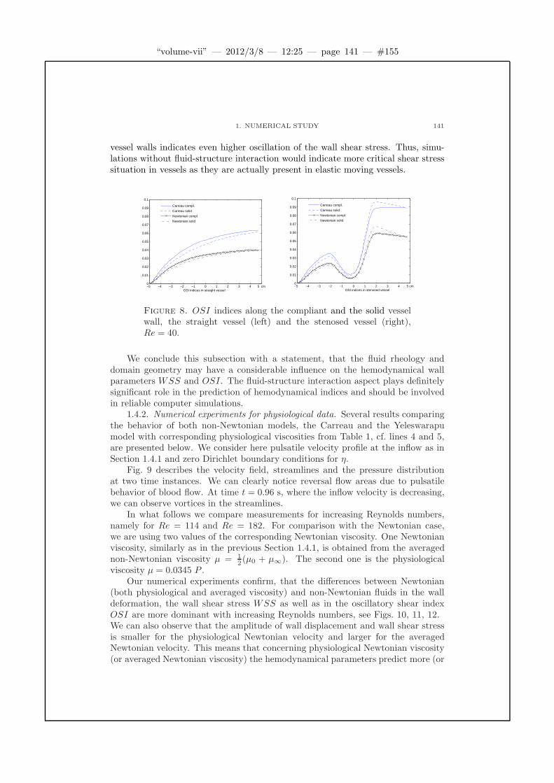
“volume-vii” — 2012/3/8 — 12:25 — page 141 — #155


vessel walls indicates even higher oscillation of the wall shear stress. Thus, simu-lations without fluid-structure interaction would indicate more critical shear stresssituation in vessels as they are actually present in elastic moving vessels.

−5 −4 −3 −2 −1 0 1 2 3 4 5 cm0

0.01

0.02

0.03

0.04

0.05

0.06

0.07

0.08

0.09

0.1

OSI indices in straight vessel

Carreau compl.

Carreau solid

Newtonian compl.

Newtonian solid

−5 −4 −3 −2 −1 0 1 2 3 4 5 cm0

0.01

0.02

0.03

0.04

0.05

0.06

0.07

0.08

0.09

0.1

OSI indices in stenosed vessel

Carreau compl.

Carreau solid

Newtonian compl.

Newtonian solid

Figure 8. OSI indices along the compliant and the solid vesselwall, the straight vessel (left) and the stenosed vessel (right),Re = 40.

We conclude this subsection with a statement, that the fluid rheology anddomain geometry may have a considerable influence on the hemodynamical wallparameters WSS and OSI. The fluid-structure interaction aspect plays definitelysignificant role in the prediction of hemodynamical indices and should be involvedin reliable computer simulations.

1.4.2. Numerical experiments for physiological data. Several results comparingthe behavior of both non-Newtonian models, the Carreau and the Yeleswarapumodel with corresponding physiological viscosities from Table 1, cf. lines 4 and 5,are presented below. We consider here pulsatile velocity profile at the inflow as inSection 1.4.1 and zero Dirichlet boundary conditions for η.

Fig. 9 describes the velocity field, streamlines and the pressure distributionat two time instances. We can clearly notice reversal flow areas due to pulsatilebehavior of blood flow. At time t = 0.96 s, where the inflow velocity is decreasing,we can observe vortices in the streamlines.

In what follows we compare measurements for increasing Reynolds numbers,namely for Re = 114 and Re = 182. For comparison with the Newtonian case,we are using two values of the corresponding Newtonian viscosity. One Newtonianviscosity, similarly as in the previous Section 1.4.1, is obtained from the averagednon-Newtonian viscosity µ = 1

2 (µ0 + µ∞). The second one is the physiologicalviscosity µ = 0.0345 P .

Our numerical experiments confirm, that the differences between Newtonian(both physiological and averaged viscosity) and non-Newtonian fluids in the walldeformation, the wall shear stress WSS as well as in the oscillatory shear indexOSI are more dominant with increasing Reynolds numbers, see Figs. 10, 11, 12.We can also observe that the amplitude of wall displacement and wall shear stressis smaller for the physiological Newtonian velocity and larger for the averagedNewtonian velocity. This means that concerning physiological Newtonian viscosity(or averaged Newtonian viscosity) the hemodynamical parameters predict more (or

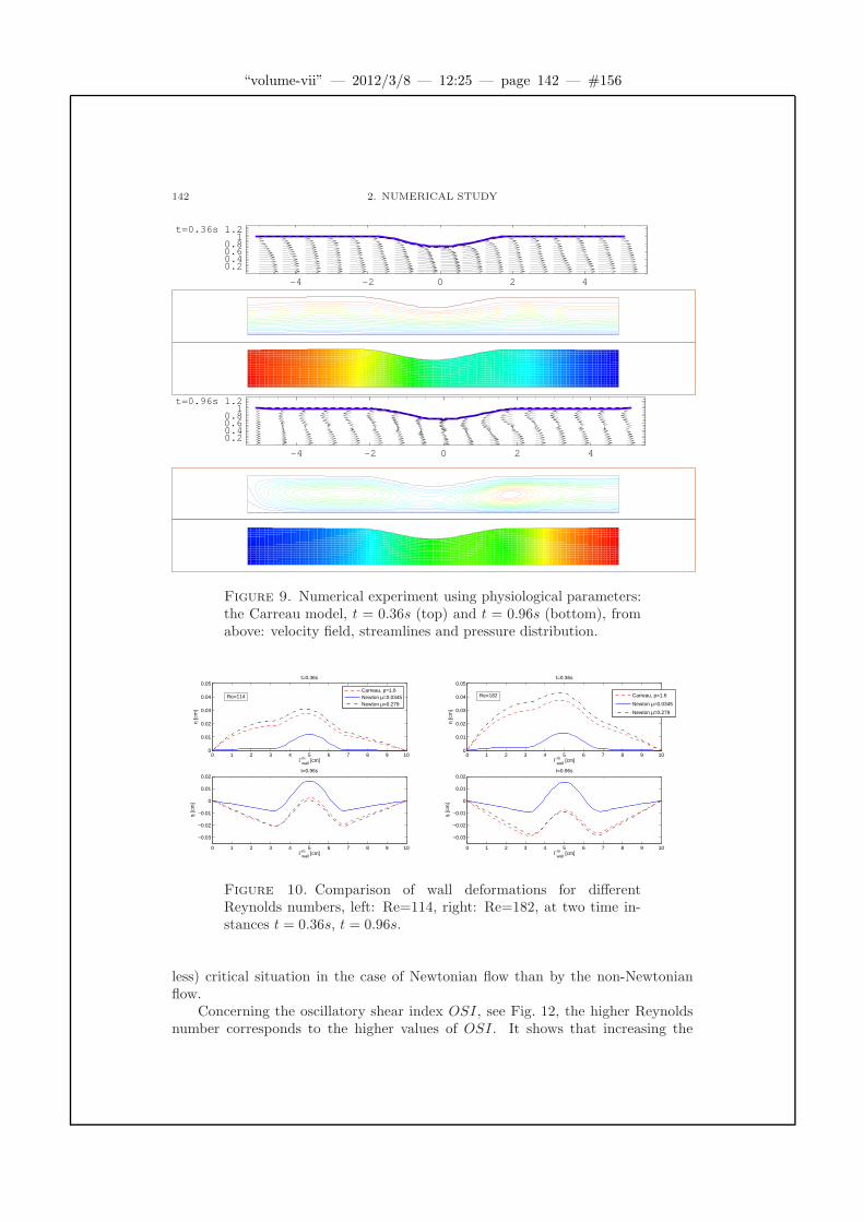
“volume-vii” — 2012/3/8 — 12:25 — page 142 — #156


-4 -2 0 2 4

0.20.40.60.81

t=0.36s 1.2

-4 -2 0 2 4

0.20.40.60.81

t=0.96s 1.2

Figure 9. Numerical experiment using physiological parameters:the Carreau model, t = 0.36s (top) and t = 0.96s (bottom), fromabove: velocity field, streamlines and pressure distribution.

0 1 2 3 4 5 6 7 8 9 100

0.01

0.02

0.03

0.04

0.05

Γwallm [cm]

η [c

m]

t=0.36s

Carreau, p=1.6Newton µ=0.0345Newton µ=0.279

0 1 2 3 4 5 6 7 8 9 10

−0.03

−0.02

−0.01

0

0.01

0.02

Γwallm [cm]

η [c

m]

t=0.96s

Re=114

0 1 2 3 4 5 6 7 8 9 100

0.01

0.02

0.03

0.04

0.05

Γwallm [cm]

η [c

m]

t=0.36s

Carreau, p=1.6

Newton µ=0.0345

Newton µ=0.279

0 1 2 3 4 5 6 7 8 9 10

−0.03

−0.02

−0.01

0

0.01

0.02

Γwallm [cm]

η [c

m]

t=0.96s

Re=182

Figure 10. Comparison of wall deformations for differentReynolds numbers, left: Re=114, right: Re=182, at two time in-stances t = 0.36s, t = 0.96s.

less) critical situation in the case of Newtonian flow than by the non-Newtonianflow.

Concerning the oscillatory shear index OSI, see Fig. 12, the higher Reynoldsnumber corresponds to the higher values of OSI. It shows that increasing the

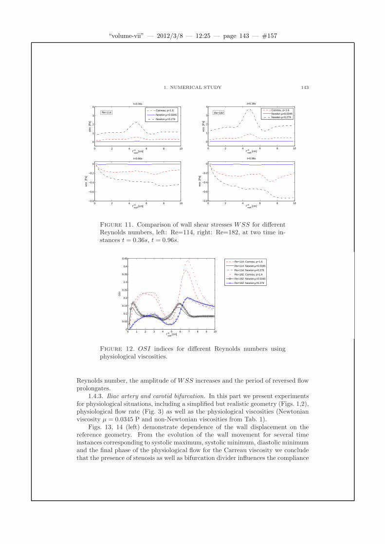
“volume-vii” — 2012/3/8 — 12:25 — page 143 — #157


0 2 4 6 8 10

0

1

2

3

4

Γwallm [cm]

wss

[P

a]

t=0.36s

Carreau, p=1.6

Newton µ=0.0345

Newton µ=0.279

0 2 4 6 8 10−0.8

−0.6

−0.4

−0.2

0

Γwallm [cm]

wss

[P

a]

t=0.96s

Re=114

0 2 4 6 8 10

0

1

2

3

4

Γwallm [cm]

wss

[P

a]

t=0.36s

Carreau, p=1.6Newton µ=0.0345Newton µ=0.279

0 2 4 6 8 10−0.8

−0.6

−0.4

−0.2

0

Γwallm [cm]

wss

[P

a]

t=0.96s

Re=182

Figure 11. Comparison of wall shear stresses WSS for differentReynolds numbers, left: Re=114, right: Re=182, at two time in-stances t = 0.36s, t = 0.96s.

0 1 2 3 4 5 6 7 8 9 100

0.05

0.1

0.15

0.2

0.25

0.3

0.35

0.4

0.45

Γwallm [cm]

OS

I

Re=114: Carreau, p=1.6

Re=114: Newton µ=0.0345

Re=114: Newton µ=0.279

Re=182: Carreau, p=1.6

Re=182: Newton µ=0.0345

Re=182: Newton µ=0.279

Figure 12. OSI indices for different Reynolds numbers usingphysiological viscosities.

Reynolds number, the amplitude of WSS increases and the period of reversed flowprolongates.

1.4.3. Iliac artery and carotid bifurcation. In this part we present experimentsfor physiological situations, including a simplified but realistic geometry (Figs. 1,2),physiological flow rate (Fig. 3) as well as the physiological viscosities (Newtonianviscosity µ = 0.0345 P and non-Newtonian viscosities from Tab. 1).

Figs. 13, 14 (left) demonstrate dependence of the wall displacement on thereference geometry. From the evolution of the wall movement for several timeinstances corresponding to systolic maximum, systolic minimum, diastolic minimumand the final phase of the physiological flow for the Carreau viscosity we concludethat the presence of stenosis as well as bifurcation divider influences the compliance

“volume-vii” — 2012/3/8 — 12:25 — page 144 — #158


of the vessel wall. Comparing the Newtonian as well as non-Newtonian rheology(Figs. 13, 14, right) we see that the difference between them is not significant.

0 1 2 3 4 5 6−0.015

−0.01

−0.005

0

0.005

0.01

0.015

0.02

Γwallm [cm]

η [c

m]

wall deformation, stenosis, Carreau

t=0.15 s

t=0.36 s

t=0.58 s

t=0.90 s

0 1 2 3 4 5 6−0.015

−0.01

−0.005

0

Γwallm [cm]

η [c

m]

wall deformation, stenosis, Carreau, t=0.36 s

Carreau, p=1.6

Yeleswarapu, Λ=14.81

Newton µ=0.0345

Figure 13. The evolution of η along the line x2 = R0 for stenosedvessel. Left: comparison at several time instances, right: compar-ison of different constitutive models at t = 0.36 s.

0 0.5 1 1.5 2 2.5

−6

−4

−2

0

2

x 10−3

Γwallm [cm]

η [c

m]

wall deformation, real. bifurcation, Carreau

t=0.1 s

t=0.23 s

t=0.36 s

t=0.96 s

0 0.5 1 1.5 2 2.5−4

−3.5

−3

−2.5

−2

−1.5

−1

−0.5

0

0.5x 10

−3

Γwallm [cm]

η [c

m]

wall deformation, real. bifurcation, Carreau, t=0.36 s

Carreau, p=1.6


Newton µ=0.0345

Figure 14. The evolution of η along the moving boundary Γmwall

for bifurcation geometry. Left: comparison at different time in-stances, right: comparison of constitutive models at t = 0.36 s.

The WSS distribution along the moving boundary for both types of geometry ispresented in Figs. 15, 16. We see that the peak of the WSS corresponds to thestenosed area (see Fig. 15) and to the bifurcation divider (see Fig. 16). In the caseof stenosed vessel we observe one reversed vortex at t = 0.36 s and two vorticesat t = 0.58 s. Moreover, at time instances t = 0.58 s and t = 0.90 s, the WSSbelongs to the athero-prone range. Looking at the bifurcation geometry (Fig. 16),a reversed flow at all time instances around the sinus bulb appears. Moreover,approaching the bifurcation divider lower values of the WSS can be found. Inboth cases, stenotic iliac and bifurcation carotid artery, we observe that the WSScorresponding to the non-Newtonian model gives higher extremal values.

In Fig. 17 the OSI index along the moving boundary for stenotic (left) andbifurcation geometry (right) is presented. Due to the high shear flow in a stenosedregion, direction-varyingWSS, in particular before and after stenosis, can be found.

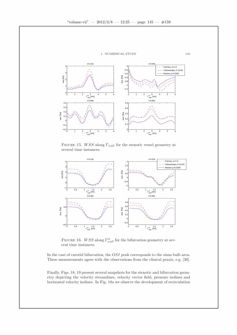
“volume-vii” — 2012/3/8 — 12:25 — page 145 — #159


0 1 2 3 4 5 60

1

2

3

4

Γwallm [cm]

wss

[Pa]

t=0.15s

0 1 2 3 4 5 6

−1.2

−1

−0.8

−0.6

−0.4

−0.2

0

Γwallm [cm]

wss

[P

a]

t=0.36s

Carreau, p=1.6


Newton µ=0.0345

0 1 2 3 4 5 6−0.2

−0.1

0

0.1

0.2

0.3

0.4

Γwallm [cm]

wss

[P

a]

t=0.58s

0 1 2 3 4 5 60

0.1

0.2

0.3

0.4

0.5

Γwallm [cm]

wss

[P

a]

t=0.90s

Figure 15. WSS along Γwall for the stenotic vessel geometry atseveral time instances.

0 0.5 1 1.5 2 2.5−1

0

1

2

3

4

Γwallm [cm]

wss

[Pa]

t=0.10s

0 0.5 1 1.5 2 2.5

−1

−0.5

0

0.5

1

1.5

2

Γwallm [cm]

wss

[P

a]

t=0.23s

Carreau, p=1.6


Newton µ=0.0345

0 0.5 1 1.5 2 2.5−0.5

0

0.5

1

Γwallm [cm]

wss

[P

a]

t=0.36s

0 0.5 1 1.5 2 2.5

−0.2

0

0.2

0.4

0.6

0.8

Γwallm [cm]

wss

[P

a]

t=0.90s

Figure 16. WSS along Γmwall for the bifurcation geometry at sev-

eral time instances.

In the case of carotid bifurcation, the OSI peak corresponds to the sinus bulb area.These measurements agree with the observations from the clinical praxis, e.g. [30].

Finally, Figs. 18, 19 present several snapshots for the stenotic and bifurcation geom-etry depicting the velocity streamlines, velocity vector field, pressure isolines andhorizontal velocity isolines. In Fig. 18a we observe the development of recirculation

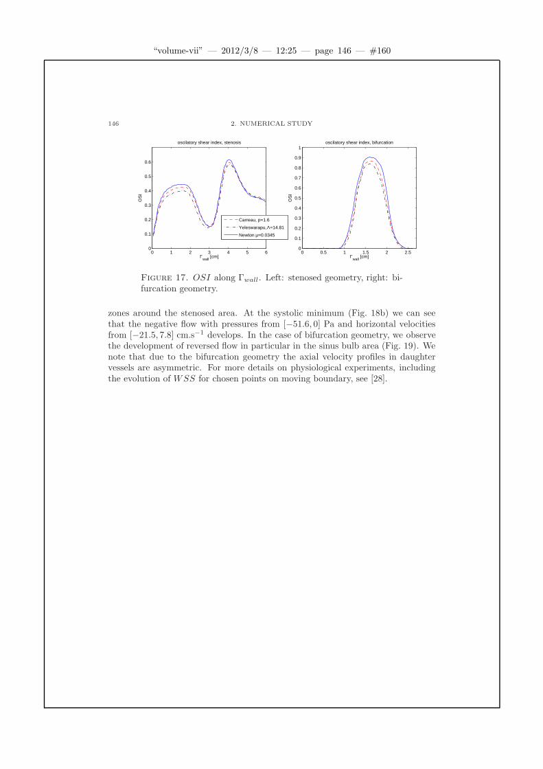
“volume-vii” — 2012/3/8 — 12:25 — page 146 — #160


0 1 2 3 4 5 60

0.1

0.2

0.3

0.4

0.5

0.6

Γwall

[cm]

OS

Ioscilatory shear index, stenosis

0 0.5 1 1.5 2 2.50

0.1

0.2

0.3

0.4

0.5

0.6

0.7

0.8

0.9

1

Γwall

[cm]

OS

I

oscilatory shear index, bifurcation

Carreau, p=1.6


Newton µ=0.0345

Figure 17. OSI along Γwall. Left: stenosed geometry, right: bi-furcation geometry.

zones around the stenosed area. At the systolic minimum (Fig. 18b) we can seethat the negative flow with pressures from [−51.6, 0] Pa and horizontal velocitiesfrom [−21.5, 7.8] cm.s−1 develops. In the case of bifurcation geometry, we observethe development of reversed flow in particular in the sinus bulb area (Fig. 19). Wenote that due to the bifurcation geometry the axial velocity profiles in daughtervessels are asymmetric. For more details on physiological experiments, includingthe evolution of WSS for chosen points on moving boundary, see [28].

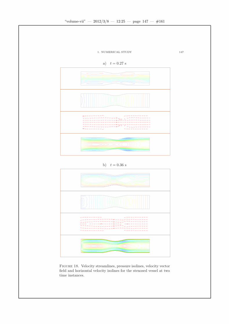
“volume-vii” — 2012/3/8 — 12:25 — page 147 — #161


a) t = 0.27 s

b) t = 0.36 s

Figure 18. Velocity streamlines, pressure isolines, velocity vectorfield and horizontal velocity isolines for the stenosed vessel at twotime instances.

“volume-vii” — 2012/3/8 — 12:25 — page 148 — #162


a) t = 0.23 s

b) t = 0.36 s

Figure 19. Velocity streamlines, velocity vector field, pressureisolines and horizontal velocity isolines for the bifurcation geometryat two time instances.

“volume-vii” — 2012/3/8 — 12:25 — page 149 — #163


1.5. Convergence study. In our numerical experiments we have used piece-wise linear approximations for fluid velocities and for pressure and backward Eulermethod for time discretization. In the case of global iterative method the structureequation is approximated by the second order Newmark method. For the kinemat-ical splitting method the second order approximation in space and time (Crank-Nicolson method) was applied. Both the first order Marchuk-Yanenko splitting aswell as the second order Strang splitting schemes have been tested.

In order to study accuracy of the coupled fluid-structure interaction problemthe so-called experimental order of convergence (EOC) is computed. TheEOC in space is defined in the following way

EOC(u) = log2‖uh,∆t − u h

2 ,∆t‖Lp/‖Ωh‖Lp

‖uh2 ,∆t − u h

4 ,∆t‖Lp/‖Ωh2‖Lp

. (1.13)

To evaluate the EOC in space, the computational domain Ω(η) is consecutivelydivided into 16×2 elements (1. refinement), 32×4 elements (2. refinement), 64×8elements (3. refinement), 128× 16 elements (4. refinement), where the element sizeh = (∆x,∆y) is halved. The space errors and the EOC were computed at T = 0.8s.The constant time step was chosen to be enough small and set to ∆t = 0.002s.

We consider here the Carreau model for non-Newtonian fluid as well as theNewtonian fluid. The index p denotes the corresponding exponent in the power-lawmodel used for the non-Newtonian Carreau viscosity function, see (2.2). In our casewe took q = −0.2, which yields p = 1.6 as well as q = 0 (p = 2) in the Newtoniancase. Note that due to the regularity results presented in Subsection 4.1.1 wemeasure the errors in the Lp, or W 1,p, norm for velocity for the non-Newtonianfluid and in the L2, or W 1,2, norm for the Newtonian fluid. Due to the artificialcompressibility regularization of the continuity equation we can measure pressurein the L2 norm.

Let us firstly present the convergence results in space in term of the EOC valuesfor velocity and pressure in a rigid domain, Tab. 3. For each quantity a followingnotation for the normalized Lp-error was used

Err(u) =‖uh,∆t − uh/2,∆t‖Lp

‖Ωh‖Lp

.

Table 3 presents convergence results in a fixed domain with the symmetry boundary

Table 3. Convergence rates in space, rigid domain.

Newtonian fluid Carreau fluid, q = −0.2

# of refin. Err(u) EOC Err(p) EOC Err(u) EOC Err(p) EOC

L2 norm Lp norm L2 norm

2/1 1.0783 3.5199 0.9083 3.72093/2 0.2758 1.967 0.6870 2.357 0.2494 1.865 0.7073 2.3954/3 0.084 1.715 0.3204 1.101 0.1092 1.192 0.1577 2.165

conditions at the central line, see Fig. 20. We can notice slightly worse thansecond order convergence rate in velocity for the Newtonian case. Moreover, inthe non-Newtonian case the convergence in velocity is reduced to 1. This effectcan be explained by the influence of symmetry boundary conditions coupled with

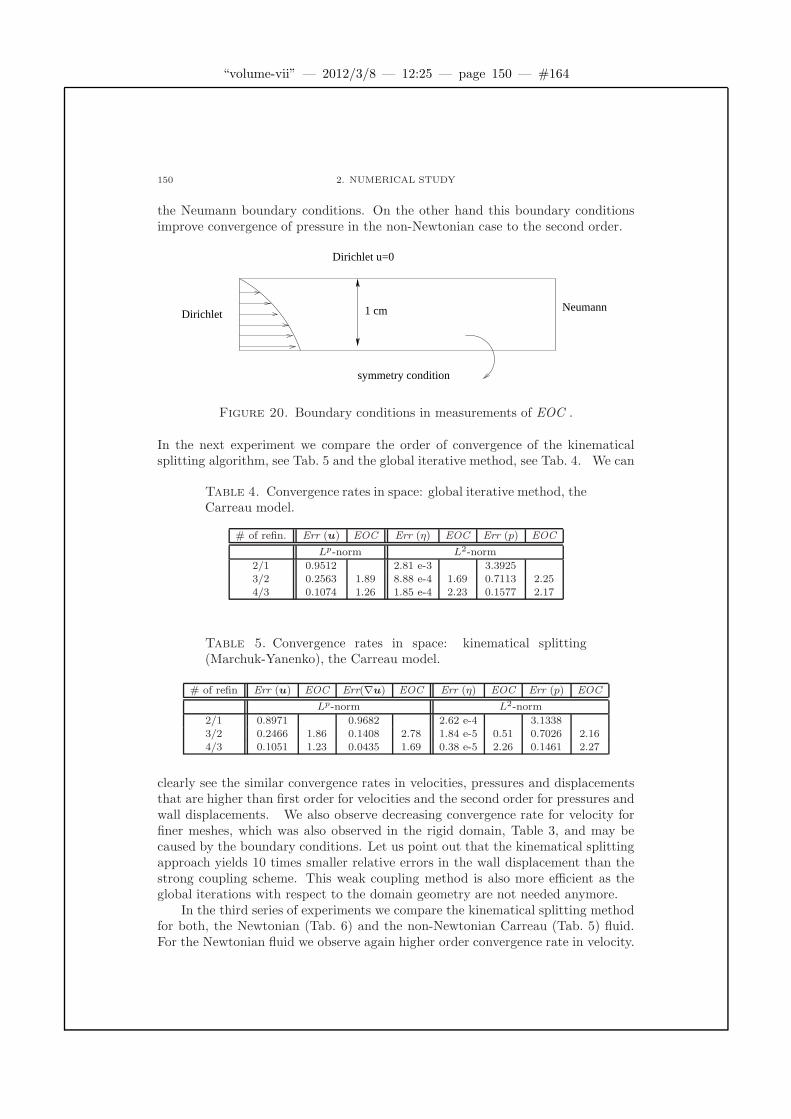
“volume-vii” — 2012/3/8 — 12:25 — page 150 — #164


the Neumann boundary conditions. On the other hand this boundary conditionsimprove convergence of pressure in the non-Newtonian case to the second order.

symmetry condition

Dirichlet u=0

DirichletNeumann1 cm

Figure 20. Boundary conditions in measurements of EOC .

In the next experiment we compare the order of convergence of the kinematicalsplitting algorithm, see Tab. 5 and the global iterative method, see Tab. 4. We can

Table 4. Convergence rates in space: global iterative method, theCarreau model.

# of refin. Err (u) EOC Err (η) EOC Err (p) EOC

Lp-norm L2-norm

2/1 0.9512 2.81 e-3 3.39253/2 0.2563 1.89 8.88 e-4 1.69 0.7113 2.254/3 0.1074 1.26 1.85 e-4 2.23 0.1577 2.17

Table 5. Convergence rates in space: kinematical splitting(Marchuk-Yanenko), the Carreau model.

# of refin Err (u) EOC Err(∇u) EOC Err (η) EOC Err (p) EOC

Lp-norm L2-norm

2/1 0.8971 0.9682 2.62 e-4 3.13383/2 0.2466 1.86 0.1408 2.78 1.84 e-5 0.51 0.7026 2.164/3 0.1051 1.23 0.0435 1.69 0.38 e-5 2.26 0.1461 2.27

clearly see the similar convergence rates in velocities, pressures and displacementsthat are higher than first order for velocities and the second order for pressures andwall displacements. We also observe decreasing convergence rate for velocity forfiner meshes, which was also observed in the rigid domain, Table 3, and may becaused by the boundary conditions. Let us point out that the kinematical splittingapproach yields 10 times smaller relative errors in the wall displacement than thestrong coupling scheme. This weak coupling method is also more efficient as theglobal iterations with respect to the domain geometry are not needed anymore.

In the third series of experiments we compare the kinematical splitting methodfor both, the Newtonian (Tab. 6) and the non-Newtonian Carreau (Tab. 5) fluid.For the Newtonian fluid we observe again higher order convergence rate in velocity.

“volume-vii” — 2012/3/8 — 12:25 — page 151 — #165


Considering the non-Newtonian rheology the convergence rate in pressure is ofthe second order. It is typically better than in the Newtonian case. Since theconvergence of η depends on the convergence rates of ∇u and p, we see in thecase of non-Newtonian rheology improvement of the convergence order for the walldisplacement, too.

Table 6. Convergence rates in space for Marchuk-Yanenko split-ting, Newtonian viscosity.

# of refin. Err (u) EOC Err(∇u) EOC Err (η) EOC Err (p) EOC

L2-norm

2/1 1.0566 1.2723 1.56e-4 3.00763/2 0.2780 1.93 0.2171 2.55 1.94e-4 -0.32 0.7081 2.094/3 0.0872 1.67 0.0483 2.17 1.12e-4 0.79 0.0313 1.18

Now we compare the convergence results in space for four possible schemes ofthe kinematical splitting method, i.e. explicit Marchuk-Yanenko splitting (Tab. 7),implicit Marchuk-Yanenko splitting (Tab. 8), explicit Strang splitting (Tab. 9) andimplicit Strang splitting (Tab. 10). As it is expected there is no significant

Table 7. Convergence rates in space; explicit Marchuk-Yanenkosplitting, the Carreau viscosity.


Lp-norm L2-norm

2/1 0.8667 0.9292 1.01 e-4 3.00973/2 0.2338 1.89 0.1283 2.86 0.66 e-5 0.61 0.6451 2.224/3 0.1032 1.18 0.0437 1.55 0.25 e-5 1.37 0.1791 1.85

Table 8. Convergence rates in space; implicit Marchuk-Yanenkosplitting, the Carreau viscosity.


Lp-norm L2-norm

2/1 1.0866 0.9470 1.04e-4 3.43323/2 0.3300 1.72 0.1626 2.54 4.26e-5 1.29 0.8190 2.074/3 0.1034 1.67 0.0442 1.88 2.51e-5 0.76 0.1960 2.06

improvement in the convergence rate in space due to the Strang splitting, howeverthe implicit scheme improves the convergence rate.

The last series of experiments focuses on the evaluation of the EOC in time,that is given as follows

EOC(u) = log2

(∑Nj=1 ||u

jh,∆t − u

jh,∆t/2||

pLp/|Ωj

h,∆t|p)1/p

(1/2

∑2Nj=1 ||u

jh,∆t/2 − u

jh,∆t/4||

pLp/|Ωj

h,∆t/2|p)1/p . (1.14)

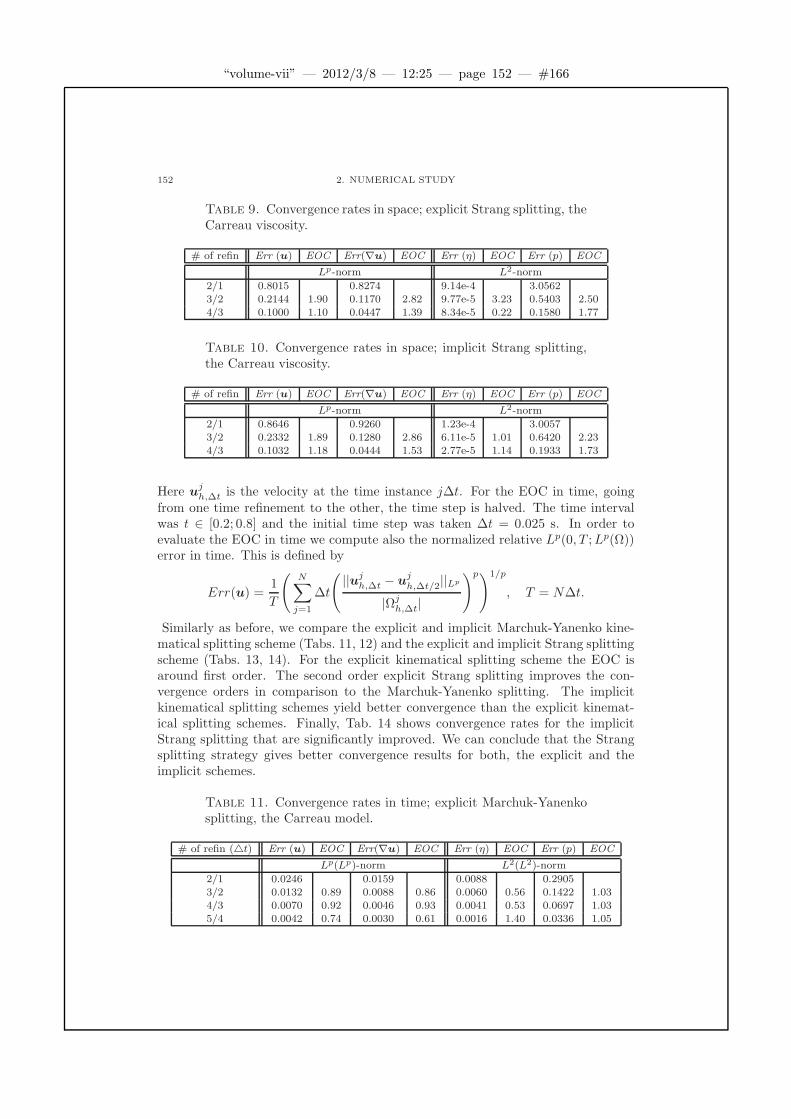
“volume-vii” — 2012/3/8 — 12:25 — page 152 — #166


Table 9. Convergence rates in space; explicit Strang splitting, theCarreau viscosity.


Lp-norm L2-norm

2/1 0.8015 0.8274 9.14e-4 3.05623/2 0.2144 1.90 0.1170 2.82 9.77e-5 3.23 0.5403 2.504/3 0.1000 1.10 0.0447 1.39 8.34e-5 0.22 0.1580 1.77

Table 10. Convergence rates in space; implicit Strang splitting,the Carreau viscosity.


Lp-norm L2-norm

2/1 0.8646 0.9260 1.23e-4 3.00573/2 0.2332 1.89 0.1280 2.86 6.11e-5 1.01 0.6420 2.234/3 0.1032 1.18 0.0444 1.53 2.77e-5 1.14 0.1933 1.73

Here ujh,∆t is the velocity at the time instance j∆t. For the EOC in time, going

from one time refinement to the other, the time step is halved. The time intervalwas t ∈ [0.2; 0.8] and the initial time step was taken ∆t = 0.025 s. In order toevaluate the EOC in time we compute also the normalized relative Lp(0, T ;Lp(Ω))error in time. This is defined by

Err(u) =1

T

(N∑

j=1

∆t

(||uj

h,∆t − ujh,∆t/2||Lp

|Ωjh,∆t|

)p)1/p

, T = N∆t.

Similarly as before, we compare the explicit and implicit Marchuk-Yanenko kine-matical splitting scheme (Tabs. 11, 12) and the explicit and implicit Strang splittingscheme (Tabs. 13, 14). For the explicit kinematical splitting scheme the EOC isaround first order. The second order explicit Strang splitting improves the con-vergence orders in comparison to the Marchuk-Yanenko splitting. The implicitkinematical splitting schemes yield better convergence than the explicit kinemat-ical splitting schemes. Finally, Tab. 14 shows convergence rates for the implicitStrang splitting that are significantly improved. We can conclude that the Strangsplitting strategy gives better convergence results for both, the explicit and theimplicit schemes.

Table 11. Convergence rates in time; explicit Marchuk-Yanenkosplitting, the Carreau model.

# of refin (t) Err (u) EOC Err(∇u) EOC Err (η) EOC Err (p) EOC

Lp(Lp)-norm L2(L2)-norm

2/1 0.0246 0.0159 0.0088 0.29053/2 0.0132 0.89 0.0088 0.86 0.0060 0.56 0.1422 1.034/3 0.0070 0.92 0.0046 0.93 0.0041 0.53 0.0697 1.035/4 0.0042 0.74 0.0030 0.61 0.0016 1.40 0.0336 1.05

“volume-vii” — 2012/3/8 — 12:25 — page 153 — #167

2. CONCLUDING REMARKS 153

Table 12. Convergence rates in time; implicit Marchuk-Yanenkoscheme the Carreau model.



2/1 0.1491 0.1633 0.1640 0.56163/2 0.1532 -0.03 0.1600 0.03 0.2706 -0.72 0.4332 0.374/3 0.0705 1.12 0.0747 1.10 0.2000 0.44 0.2286 0.925/4 0.0218 1.69 0.0234 1.67 0.0915 1.13 0.0683 1.74

Table 13. Convergence rates in time; explicit Strang splitting,the Carreau model.



2/1 0.0564 0.0252 0.0583 0.33633/2 0.0195 1.53 0.0081 1.65 0.0234 1.32 0.1539 1.134/3 0.0077 1.34 0.0024 1.75 0.0089 1.40 0.0712 1.115/4 0.0044 0.83 0.0013 0.90 0.0054 0.72 0.0315 1.18

Table 14. Convergence rates in time; implicit Strang splitting,the Carreau model.



2/1 0.1826 0.1936 0.2211 0.59693/2 0.0578 1.66 0.0609 1.67 0.1140 0.96 0.2411 1.314/3 0.0241 1.26 0.0243 1.32 0.0441 1.37 0.0896 1.435/4 0.0088 1.44 0.0078 1.64 0.0173 1.35 0.0297 1.60

2. Concluding remarks

In this overview paper we have summarized our recent results on mathemat-ical modelling and numerical simulation of fluid-structure interaction of a shear-dependent non-Newtonian fluid and a viscoelastic membrane. We have presentedmathematical models for both the shear-dependent fluids and the generalized stringequation. Further, we have derived two fluid-structure interaction methods, theglobal iterative method belonging to the class of strongly coupled schemes, andthe kinematical splitting which is a weakly coupled method. The global iterativemethod has been also used in order to prove existence of a weak solution to fullycoupled interactions between the shear-dependent fluids and the viscoelastic struc-ture. As far as we know the result presented in [25] is the first contribution to thewell-posedness of fluid-structure interaction for non-Newtonian fluids.

The kinematical splitting yields a numerical scheme that is more efficient thanthe global iterative method while having typically smaller global errors. We haveanalysed stability of the semi-discrete kinematical splitting method and shown thatdepending on the choice of discretization for the ALE convective term we mayobtain a semi-discrete scheme that does or does not depend on a time step. Indeed,using the implicit Euler time discretization we obtain the stability condition for time

“volume-vii” — 2012/3/8 — 12:25 — page 154 — #168


step depending on a mesh velocity. If the midpoint rule is used in order to discretizethe ALE convective term the semi-discrete kinematical splitting is unconditionallystable, cf. also [28].

An application which is of particular interest is blood flow in elastic vessels.We have simulated blood flow in a stenotic vessel and a carotid bifurcation andanalyzed some hemodynamical control quantities. We have modeled blood as ashear-thinning non-Newtonian fluid and chosen two well-known models, the Carreaumodel and the Yeleswarapu model. Comparisons with the Newtonian model arepresented as well.

Further, we have investigated the wall deformation and the hemodynamicalwall parameters, the wall shear stress WSS and the oscillatory shear index OSI,for a straight and stenotic vessel as well as for a carotid bifurcation. Numericalsimulations demonstrate a significant influence of the non-Newtonian rheology forhemodynamical wall parameters. According to some authors [31] negative valuesof WSS indicates occurance of recirculation zones and reversal flows around steno-sis, which seems to be better predicted by the non-Newtonian models. Further,the domain geometry has also a considerable influence on the wall deformation aswell as on the WSS and OSI. The maximum values of OSI are larger for theNewtonian fluid. Such high OSI values at the end of stenotic occlusion indicate alarge oscillatory nature of the wall shear stress and could yield further to additionalstenotic plug.

Comparisons of WSS and OSI for a solid and compliant vessel showed sig-nificantly higher oscillations of the wall shear stress for fixed solid vessels. Thisleads to the conclusion that the fluid-structure interaction aspect is important forhemodynamical modelling and should be involved in reliable computational models.

It would be interesting to extend mathematical models and consider the gen-eralized Oldroyd-B model that includes viscoelastic properties of blood as well.More realistic models for vessel walls, see, e.g., [6], allowing deformation in bothdirections would be more appropriate in order to consider more complex vessel ge-ometries. An important point of numerical simulation is a correct outflow boundarycondition, reflecting the influence of the rest of circulatory system. According to[45] this can be realized by the so-called impedance condition arising from couplingthe fluid equations with some less dimensional model (1D or 0D lumped model).

“volume-vii” — 2012/3/8 — 12:25 — page 155 — #169

Bibliography

[1] Bastian P., Johannsen K., Reichenberger V.: UG tutorial, 2001.[2] Bodnar T., Sequeira A.: Numerical study of the significance of the non-

Newtonian nature of blood in steady flow through a stenosed vessel, In: Ran-nacher R. et.al. (Eds.), Advances in Mathematical Fluid Mechanics, 83–104,Springer Verlag, 2010.

[3] Broser Ph. J.: Simulation von Stromungen in Blutgefassen, Master Thesis,Ruprechts-Karl University, Heidelberg, 2001.

[4] Bucur D., Fereisl E., Necasova S.: Influence of wall roughness on the slipbehavior of viscous fluids, Proc. R. Soc. Edinb., Sect. A, Math. 138(5) (2008),957-973.

[5] Bucur D., Feireisl E., Necasova S., Wolf J.: On the asymptotic limit of theNavier-Stokes system on domains with rough boundaries, J. of Differ. Equa-tions 244 (2008), 2890–2908.

[6] Canic S., Tambaca J., Guidoboni G., Mikelic A., Hartley C.J., RosenstrauchD.: Modeling viscoelastic behavior of arterial walls and their intercation withpulsatile blood flow, SIAM J. Appl. Math. 67(1) (2006), 164–193.

[7] Chambolle A., Desjardin B., Esteban M.J., Grandmont C.: Existence of weaksolutions for unsteady fluid-plate interaction problem, J. Math. Fluid Mech. 7(3) (2005), 368–404.

[8] Cerny J.: Numerical modelling of non-Newtonian flows with application inhemodynamics, Report TU Hamburg-Harburg, 2004.

[9] Cheng A., Shkoller S.: The interaction of the 3D Navier-Stokes equations witha moving nonlinear Koiter elastic shell, SIAM J. Math. Anal. 42(3) (2010),1094-1155.

[10] Cheng A., Coutand D., Shkoller S.: Navier-Stokes equations interacting witha nonlinear elastic biofluid shell, SIAM J. Math. Anal. 39(3) (2007), 742-800.

[11] Coutand D., Shkoller S.: Motion of an elastic solid inside an incompressibleviscous fluid, Arch. Ration. Mech. Anal. 176(1) (2005), 25-102.

[12] Coutand D., Shkoller S.: Interaction between quasilinear elasticity and theNavier-Stokes equations, Arch. Ration. Mech. Anal. 179 (2006), 303-352.

[13] Filo J., Zauskova A.: 2D Navier-Stokes equations in a time dependent domainwith Neumann type boundary conditions, J. Math. Fluid Mech. 10 (2008),1–46.

[14] Formaggia L., Gerbeau J.F., Nobile F., Quarteroni A.: On the coupling of3D and 1D Navier-Stokes equations for flow problems in compliant vessels,Comput. Meth. Appl. Mech. Eng. 191 (6-7) (2001), 561–582.

155

“volume-vii” — 2012/3/8 — 12:25 — page 156 — #170

156 BIBLIOGRAPHY

[15] Formaggia L., Nobile F.: A stability analysis for the arbitrary LagrangianEulerian formularion with finite elements, East-West J. Numer. Math. 7 (2)(1999), 103–131.

[16] Forster C., Scheven von M., Wall W.A., Ramm E.: Coupling of incompressibleflows and thin-walled structures, In: Papadrakakis M. et. al. (Eds.) Coupled

Problems 2007 International Conference on Computational Methods for Cou-

pled Problems in Science and Engineering, 541–544, Greece, 2007.[17] Frehse J., Malek J., Steinhauer M.: On analysis of steady flow of fluid with

shear dependent viscosity based on the Lipschitz truncation method, SIAM J.

Math. Anal. 35(5) (2003), 1064–1083.[18] Galdi G.P., Rannacher R., Robertson A.M., Turek S.: Hemodynamical Flows.

Modeling, Analysis, Simulation., Oberwolfach Seminars Vol. 37, BirkhauserVerlag, 2008.

[19] Gijsen F.J.H., van de Vosse F.N., Janssen J.D.: Influence of the non-Newtonianproperties of blood flow on the flow in large arteries: steady flow in a carotidbifurcation model, J. Biomech. 32 (1999), 601–608.

[20] Grandmont C.: Existence of weak solutions for the unsteady interaction of aviscous fluid with an elastic plate, SIAM J. Math. Anal. 40(2) (2008), 716-737.

[21] Guidoboni G., Glowinski R., Cavallini N., Canic S.: Stable-loosely coupled-type algorithm for fluid-structure interaction on blood flow, J. Comput. Phys.

228 (18) (2009) 6916–6937.[22] Guidoboni G., Guidorzi M., Padula M.: Continuous dependence on initial

data in fluid-structure motion, J. Math. Fluid Mech. (2010) published online:http://dx.doi.org/10.1007/s00021-010-0031-0.

[23] Guidorzi M., Padula M., Plotnikov P.I.: Hopf solutions to a fluid-elastic inter-action model, Math. Models Meth. Appl. Sci. 18 (2) (2008), 215–270.

[24] Hundertmark-Zauskova A., Lukacova-Medvid’ova M.: Numerical study ofshear-dependent non-Newtonian fluids in compliant vessels, Comput. Math.

Appl. 60 (2010), 572–590.[25] Hundertmark-Zauskova A., Lukacova-Medvid’ova M., Necasova S.: On the

existence of a weak solution to the coupled fluid-structure interaction problemfor the non-Newtonian shear-dependent fluid, Preprint University of Mainz,2011.

[26] Lesoinne M., Farhat Ch.: Geometric conservation laws for flow problems withmoving boundaries and deformable meshes and their impact on aeroelasticcomputations, Comput. Meth. Appl. Mech. Eng. 134 (1996), 71–90.

[27] Lukacova-Medvid’ova M., Cerny J.: Numerical modelling of non-Newtonianshear-thinning viscoelastic fluids with application in hemodynamics, In: Se-queira A. et.al. (Eds.) Proceedings of the Second International Symposium

Modelling of Physiological Flows, Portugal, 2005.[28] Lukacova-Medvid’ova M., Rusnakova G.: Kinematical splitting algorithm for

fluid-structure interaction in hemodynamics, Preprint University of Mainz &

University of Kosice, 2011.[29] Lukacova-Medvid’ova M., Zauskova A.: Numerical modelling of shear-thinning

non-Newtonian flows in compliant vessels, Int. J. Numer. Methods Fluids, 56(2008), 1409–1415.

“volume-vii” — 2012/3/8 — 12:25 — page 157 — #171

BIBLIOGRAPHY 157

[30] Malek A.M., Alper A.L., Izumo S.: Hemodynamic shear stress and its role inatherosclerosis, J. Am. Med. Assoc. 282 (1999), 2035–2042.

[31] Nadau L., Sequeira A.: Numerical simulations of shear dependent viscoelasticflows with a combined finite element - finite volume method, Comput. Math.

Appl. 53 (2007), 547–568.[32] Nagele S.: Mehrgitterverfahren fur incompressiblen Navier-Stokes Gleichungen

im laminaren und turbulenten Regime unter Berucksichtigung verschiedener

Stabilisierungsmethoden, PhD Thesis, Ruprechts-Karl University, Heidelberg,2003.

[33] Neustupa J.: Existence of weak solution to the Navier-Stokes equation in ageneral time-varying domain by Rothe method, Math. Methods Appl. Sci.

32(6) (2009), 653–683.[34] Malek J., Necas J., Ruzicka M.: On the weak solutions to a class of non-

Newtonian incompressible fluids in bounded three-dimensional domans: thecase p ≥ 2, Adv. Differ. Equat. 6(3) (2001), 257–302.

[35] Malek J., Necas J., Rokyta M., Ruzicka M.: Weak and Measure-Valued Solu-

tions to Evolutionary PDEs, Chapman and Hall, London, 1996.[36] Nobile F.: Numerical Approximation of Fluid-Structure Interaction Problems

with Application to Haemodynamics, PhD Thesis, EPFL Lausanne, 2001.[37] Perktold K., Rappitsch G.: Mathematical modelling of local arterial flow and

vessel mechanics, In: Crolet J.-M. et.al. (Eds.) Computational Methods for

Fluid-Structure Interaction, 230–245, Longman, Harlow, 1994.[38] Perktold K., Resch M., Reinfried O.P.: Three-dimensional analysis of pulsative

flow and wall shear stress in the carotid artery bifurcation, J. Biomech. 24(6)(1991), 409–420.

[39] Quarteroni A.: Mathematical and numerical simulation of the cardiovascularsystem, In: Proceedings of the International Congress of Mathematicians, Vol.

III, 839–849, Higher Ed. Press, Beijing, 2002.[40] Quarteroni A., Formaggia L.: Mathematical modelling and numerical simula-

tion of the cardiovascular system, In: Ciarlet P.G. et. al. (Eds.) Handbook of

Numerical Analysis, Elsevier, Amsterdam, 2002.[41] Quarteroni A., Gianluigi R.: Optimal control and shape optimization of aorto-

coronaric bypass anastomoses, M3AS, Math. Models Methods Appl. Sci. 13(12) (2003), 1801–1823.

[42] Quarteroni A., Valli A.: Numerical Approximation of Partial Differential Equa-

tions, Springer Verlag, 2008.[43] Rajagopal K., Lawson J.: Regulation of hemostatic system function by bio-

chemical and mechanical factors, Modeling of Biological Materials, In: BellomoN. (Ed.) Modeling and Simulation in Science, Engineering and Technology,179–201, Birkhauser, Boston, 2007.

[44] Surulescu C.: On the stationary interaction of a Navier-Stokes fluid with anelastic tube wall, Appl. Anal. 86(2) (2007), 149–165.

[45] Taylor Ch.A., Vignon-Clementel I.E., Figueroa C.A., Jansenca K.E.: Outflowboundary conditions for three-dimensional finite element modeling of bloodflow and pressure in arteries, Comput. Meth. Appl. Mech. Eng. 195 (2006),3776–3796.

“volume-vii” — 2012/3/8 — 12:25 — page 158 — #172

158 BIBLIOGRAPHY

[46] Taylor Ch.A.., Hughes J.R., Zarins C.K.: Effect of exercise on hemodynamicconditions in the abdominal aorta, J. Vasc. Surg., 29 (6) (1999), 1077–1089.

[47] Beirao da Veiga H.: On the existence of strong solution to a coupled fluid-structure evolution problem, J. Math. Fluid Mech. 6 (1) (2001), 21–52.

[48] Yeleswarapu K.K.: Evaluation of Continuum Models for Chatacterizing the

Constitutive Behavior of Blood, PhD Thesis, University of Pittsburg, 1996.[49] Yeleswarapu K.K., Kameneva M.V., Rajagopal K.R., Antaki J.F.: The flow of

blood in tubes: theory and experiments, Mech. Res.Commun. 25 (3) (1998),257–262.

[50] Wolf J.: Existence of weak solution to the equations of non stationary motionof non-Newtonian fluids with shear rate dependent viscosity, J. Math. Fluid

Mech. 9 (2007) 104–138.[51] Zauskova A.: 2D Navier-Stokes Equations In a Time Dependent Domain, PhD

Thesis, Comenius University, Bratislava, 2007.

“volume-vii” — 2012/3/8 — 12:25 — page 159 — #173

Part 5

Analysis in Orlicz spaces

Ron Kernan

“volume-vii” — 2012/3/8 — 12:25 — page 160 — #174

2000 Mathematics Subject Classification. Primary 46E35, 35J65

Key words and phrases. Orlicz spaces, gauge norms, duality, decreasingrearrangement, rearrangement invariance, elliptic partial differential equations

Abstract. The purpose of these notes is to present in a direct manner thetheory of a class of function spaces introduced and investigated by WladyslavOrlicz in the 1930’s. The theory is then applied to certain nonlinear ellipticboundary value problems.

Acknowledgement. The author is grateful to the Necas Center—in partic-ular to Josef Malek and Lubos Pick—for the opportunity to give the lectures.He would like to thank Martin Francu, Colin Phipps and Susanna Spektor fortheir help in preparing these notes.

“volume-vii” — 2012/3/8 — 12:25 — page 161 — #175

Contents

Chapter 1. Analysis in Orlicz spaces 1631. Introduction 1632. The Orlicz class LΦ(Ω) 1653. The completeness of LΦ(Ω) 1704. Duality 1715. The rearrangement invariance of LΦ(Ω) 1756. The role of Orlicz spaces in the theory of elliptic PDE 178

Bibliography 185

161

“volume-vii” — 2012/3/8 — 12:25 — page 162 — #176

“volume-vii” — 2012/3/8 — 12:25 — page 163 — #177

CHAPTER 1

Analysis in Orlicz spaces

1. Introduction

The purpose of these notes is to present in a direct manner the theory of aclass of function spaces introduced and investigated by Wladyslaw Orlicz in the1930’s. Their goal is to facilitate the application of these spaces to problems inpartial differential equations.

Orlicz had in mind the application of his spaces to the convergence of orthogonalseries. Thus, it seems appropriate to begin by describing how they arise in the studyof classical Fourier series.

First, we recall that for measurable f : Ω → R, Ω ⊂ Rn, and 1 ≤ p <∞,

‖f‖p,Ω :=

[∫

Ω

|f(x)|p dx] 1

p

,

while

‖f‖∞,Ω := ess supx∈Ω |f(x)| .It is well-known that

Lp(Ω) :=f : Ω → R : ‖f‖p,Ω <∞

is a Banach space under the norm ‖ ‖p,Ω.The connection of the Lp spaces to Fourier series is as follows. Given f ∈ L1(I),

I = [−π, π], its Fourier series is

a02

+

∞∑

k=1

ak cos kx+ bk sin kx,

in which

ak =1

π

∫ π

−π

f(y) cos ky dy, k = 0, 1, . . .

and

bk =1

π

∫ π

−π

f(y) sin ky dy, k = 1, 2, . . . .

Now, the pointwise convergence of the Kth partial sum of the Fourier series of f ,namely

(SKf)(x) :=a02

+

K∑

k=1

ak cos kx+ bk sinkx,

163

“volume-vii” — 2012/3/8 — 12:25 — page 164 — #178

164 1. ANALYSIS IN ORLICZ SPACES

to f(x), f(x−o)+f(x+o)2 or anything else was found to be difficult to prove. To

overcome this problem other kinds of convergence were considered. Thus, J. P.Gram in 1883 showed that for suitable f

limK→∞

∫ π

−π

|f(x)− (SKf)(x)|2 dx = 0;

that is, SKf converges to f in L2(I).This was later refined in 1907 by F. Riesz and E. Fischer to the assertion that,

in our notation,

limK→∞

‖f − SKf‖2,I = 0

if and only if f ∈ L2(I). Then, in 1927, M. Riesz proved that, for 1 < p <∞,

limK→∞

‖f − SKf‖p,I = 0 (1.1)

if and only if f ∈ Lp(I). However, there are functions f ∈ L1(I) and g ∈ L∞(I)such that

limK→∞

‖f − SKf‖1,I 6= 0

and

limK→∞

‖g − SKg‖∞,I 6= 0.

One may ask if there is a condition stronger than∫ π

−π

|f(x)| dx <∞

that guarantees (1.1) when p = 1. A. Zygmund, in 1928, showed that such acondition is ∫ π

−π

|f(x)| log+ |f(x)| dx <∞.

As will be seen later, this is the condition for f to belong to the Orlicz spaceL logL(I).

When p = ∞, we don’t ask if there is a condition stronger than

‖f‖∞,I = ess supx∈Ω |f(x)| <∞that guarantees (1.1), but rather if there is a norm smaller than ‖ ‖∞,I in whichwe have convergence as in (1.1) for all g ∈ L∞(I). There is indeed such a norm,namely the one for the Orlicz space Lexp(I), to which g belongs if and only if

∫ π

−π

exp(k |g(x)|)dx <∞ (1.2)

for some k > 0. Observe that every function in L∞(I) is in Lexp(I), as is theunbounded function g(x) := log π

|x| , since any k < 1 works in (1.2).

We conclude this introductory section by considering the more recent applica-tion of Orlicz spaces to Sobolev-type imbeddings. In them Ω will be a boundeddomain in Rn, a domain being an open connected set. The simplest case of theclassical Sobolev imbedding inequality asserts that

[∫

Ω

|u(x)|q dx] 1

q

≤ C

[∫

Ω

|(∇u)(x)|p dx] 1

p

(1.3)

“volume-vii” — 2012/3/8 — 12:25 — page 165 — #179

2. THE ORLICZ CLASS LΦ(Ω) 165

for all u ∈ C∞0 (Ω). Here,

∇ :=

(∂

∂x1,∂

∂x2, . . . ,

∂

∂xn

)

is the usual gradient operator,

|(∇u)(x)| :=√(

∂u

∂x1

)2

+

(∂u

∂x2

)2

+ · · ·+(∂u

∂xn

)2

and1

q=

1

p− 1

n,

where 1 < p < n. Gagliardo and Nirenberg, independently, showed the result holdsfor p = 1.

When p = n, 1q = 0. One might expect that

ess supx∈Ω |u(x)| ≤ C

[∫

Ω

|(∇u)(x)|n dx] 1

n

.

This is not the case. A norm smaller than that of L∞(Ω) is needed.In the early 1960’s, Yudovich, Pohozhaev and Trudinger each showed, Yudovich

being the first, that, when n = 2, the norm of L∞(Ω) should be replaced by thatof the Orlicz space Lexp(t2)(Ω). Strichartz later showed that for n > 2 the correctnorm is that of L

exp(tn

n−1 )(Ω). Of course, f ∈ L

exp(tn

n−1 )(Ω) if and only if

∫

Ω

exp([k |f(x)|] n

n−1

)dx <∞

for some k > 0.This so-called limiting Sobolev inequality was used by the above-mentioned

authors to prove the existence of eigenvalues for the Laplace operator.

2. The Orlicz class LΦ(Ω)

As we saw in the examples in the previous section, membership in an Orliczspace is equivalent to a condition of the form∫

Ω

Φ (k |f(x)|) dx <∞ (2.1)

for some k > 0. Often, (2.1) holds for all k > 0 if and only if it holds for one such k.In the Lp case, Φ(t) = Φp(t) = tp. Since we’ll be generalizing Lp spaces we

begin by asking what special properties Φp has when 1 < p <∞. The key property,it turns out, is

Φp(t) =

∫ t

0

psp−1ds,

where φp(s) := psp−1 increases strictly from φp(0) = 0 to ∞ as s→ ∞.

Definition 2.1. The function Φ : R+ → R+, R+ := (0,∞), is said to be aYoung function provided

Φ(t) :=

∫ t

0

φ(s)ds,

“volume-vii” — 2012/3/8 — 12:25 — page 166 — #180


in which φ : R+ → R+ is increasing and, say, left continuous, with φ(0+) = 0 andlimt→∞ φ(t) = ∞.

We observe that Φ is convex, that is, if α, β ≥ 0,α+ β = 1, then,

Φ (αt1 + βt2) ≤ αΦ(t1) + βΦ(t2).

Indeed, the point (αt1 + βt2, αΦ(t1) + βΦ(t2)) is on the line

y = Φ(t1) +Φ(t2)− Φ(t1)

t2 − t1(t− t1) = Φ(t1) +

1

t2 − t1

∫ t2

t1

φ(s)ds(t− t1)

joining (t1,Φ(t1)) and (t2,Φ(t2)) and that line lies above the graph of

y = Φ(t) = Φ(t1) +1

t− t1

∫ t

t1

φ(s)ds(t− t1),

since the average value of φ on [t1, t], namely

1

t− t1

∫ t

t1

φ(s)ds,

incerases on [t1, t2].

Example 2.2.

(1) The Orlicz norm of LlogL is given in terms of

Φ(t) =

∫ t

0

log (s+ 1)ds = (t+ 1)log(t+ 1)− t, t ∈ R+.

(2) The Orlicz norm of Lexp is defined through

Φ(t) =

∫ t

0

(es − 1)ds = et − t− 1, t ∈ R+.

Definition 2.3. Let Φ be a Young function. Then, the corresponding gauge

norm at a measurable function f : Ω → R, Ω ⊂ Rn, is

‖f‖Φ,Ω := inf

λ > 0 :

∫

Ω

Φ

( |f(x)|λ

)dx ≤ 1

.

Example 2.4.

(1) Consider Φ = Φp, 1 < p <∞. Then,∫

Ω

Φp

( |f(x)|λ

)dx =

∫

Ω

( |f(x)|λ

)p

dx ≤ 1

if and only if ∫

Ω

|f(x)|p dx ≤ λp

or [∫

Ω

|f(x)|p dx] 1

p

≤ λ.

So,

‖f‖Φp,Ω=

[∫

Ω

|f(x)|p dx] 1

p

= ‖f‖p,Ω .

“volume-vii” — 2012/3/8 — 12:25 — page 167 — #181


(2) Let Ω and E be measurable subsets of Rn, with E ⊂ Ω, |E| <∞. Denoteby χE the characteristic function of E.

Then, for any Young function Φ,

‖χE‖Φ,Ω =1

Φ−1(|E|−1).

Indeed,

1 ≥∫

Ω

Φ

(χE(x)

λ

)dx =

∫

E

Φ

(1

λ

)dx = Φ

(1

λ

)|E|

amounts to

λ ≥ 1

Φ−1(|E|−1

) ,

whence

‖χE‖Φ,Ω =1

Φ−1(|E|−1

) ,

as claimed.

Remark 2.5. Suppose ‖f‖Φ,Ω is finite and positive. Then, there exists a

strictly decreasing sequence λn in R+ such that λn ↓ ‖f‖Φ,Ω. This means that|f(x)|λn

↑ |f(x)|‖f‖Φ,Ω

, so, by the Monotone Convergence Theorem,

∫

Ω

Φ

(|f(x)|‖f‖Φ,Ω

)dx = lim

n→∞

∫

Ω

Φ

( |f(x)|λn

)dx ≤ 1.

Moreover, if∫ΩΦ(

|f(x)|λ

)dx < ∞ for λ ∈ R+, as is the case for simple functions

f , then, by the same theorem,∫

Ω

Φ

(|f(x)|‖f‖Φ,Ω

)dx = 1.

Finally, ‖f‖Φ,Ω = 0 implies∫ΩΦ

(|f(x)|

λ

)dx ≤ 1 for all λ > 0, which implies f = 0

a. e.; otherwise there would exist k > 0 and E ⊂ Ω, |E| > 0, with |f(x)| ≥ k on Eor

Φ

(k

λ

)|E| =

∫

Ω

Φ

(kχE

λ

)dx ≤

∫

Ω

Φ

( |f(x)|λ

)dx ≤ 1,

that is,

|E| ≤ 1

Φ(kλ

) , λ ∈ R+,

or |E| = 0, a contradiction.

Definition 2.6. Let Ω ⊂ Rn be measurable and suppose Φ is a Young function.The Orlicz class LΦ(Ω) is then defined as the set

f : Ω → R : ‖f‖Φ,Ω <∞

.

Proposition 2.7. Let Ω ⊂ Rn be measurable and suppose Φ is a Young func-tion. Then,

“volume-vii” — 2012/3/8 — 12:25 — page 168 — #182


(1) f ∈ LΦ(Ω), c ∈ R implies cf ∈ LΦ(Ω), with

‖cf‖Φ,Ω = |c| ‖f‖Φ,Ω ;

(2) f, g ∈ LΦ(Ω) implies f + g ∈ LΦ(Ω), with

‖f + g‖Φ,Ω ≤ ‖f‖Φ,Ω + ‖f‖Φ,Ω .

Proof. Only the second item needs proving. One may assume ‖f‖Φ,Ω > 0,

‖g‖Φ,Ω > 0. Set γ := ‖f‖Φ,Ω + ‖g‖Φ,Ω, α :=‖f‖Φ,Ω

γ and β :=‖g‖Φ,Ω

γ , so that

α, β > 0, α+ β = 1. One has

∫

Ω

Φ

( |f + g|γ

)dx ≤

∫

Ω

Φ

( |f |+ |g|γ

)dx

=

∫

Ω

Φ

(α|f |

‖f‖Φ,Ω

+β|g|

‖g‖Φ,Ω

)dx

≤∫

Ω

[αΦ

(|f |

‖f‖Φ,Ω

)+ βΦ

(|g|

‖g‖Φ,Ω

)]dx

= α

∫

Ω

Φ

(|f |

‖f‖Φ,Ω

)dx+ β

∫

Ω

Φ

(|g|

‖g‖Φ,Ω

)dx

≤ α+ β

= 1.

We conclude that‖f + g‖Φ,Ω ≤ γ = ‖f‖Φ,Ω + ‖g‖Φ,Ω .

Proposition 2.7 shows that LΦ(Ω) is a normed linear space under the functionalf → ‖f‖Φ,Ω. We next establish further poperties of this functional that will enable

us to prove, in the next section, that LΦ(Ω) is complete and thus a Banach space.

Proposition 2.8. Let Ω ⊂ Rn be measurable and suppose Φ is a Young func-tion. Then, 0 ≤ fk ↑ f a. e. on Ω implies

‖fk‖Φ,Ω ↑ ‖f‖Φ,Ω .

Proof. We first show ‖fk‖Φ,Ω ≤ ‖fk+1‖Φ,Ω , k = 1, 2, . . . . Indeed,

∫

Ω

Φ

(fk

‖fk+1‖Φ,Ω

)dx ≤

∫

Ω

Φ

(fk+1

‖fk+1‖Φ,Ω

)dx ≤ 1,

so‖fk‖Φ,Ω ≤ ‖fk+1‖Φ,Ω

Next, let αk = ‖fk‖Φ,Ω and put α = supk αk. Since f ≥ fk we have ‖f‖Φ,Ω ≥‖fk‖Φ,Ω for each k, whence ‖f‖Φ,Ω ≥ α. We need only show equality holds. Thisis clear if α = 0 or α = ∞, so we assume 0 < αk ≤ α <∞. In that case,

∫

Ω

Φ

(fkα

)dx ≤

∫

Ω

Φ

(fkαk

)dx ≤ 1

“volume-vii” — 2012/3/8 — 12:25 — page 169 — #183


and the Monotone Convergence Theorem shows

∫

Ω

Φ

(f

α

)dx ≤ 1

and hence

‖f‖Φ,Ω ≤ α.

The property of ‖ ‖Φ,Ω embodied in Proposition 2.8 is called the Fatou Prop-erty.

Proposition 2.9. Let Ω ⊂ Rn be measurable and suppose Φ is a Young func-

tion. Then, given measurable E ⊂ Ω, with 0 < |E| < ∞, there exists a positiveconstant K = KE, independent of f , such that

∫

E

|f |dx ≤ K ‖f‖Φ,Ω .

Proof. It suffices to consider f with 0 < ‖f‖Φ,Ω < ∞. Jensen’s inequality,which asserts that

Φ

(1

|E|

∫

E

|g|dx)

≤ 1

|E|

∫

E

Φ (|g|) dx,

is a simple consequence of the convexity of Φ. In particular, given k = ‖f‖−1Φ,Ω, one

has

Φ

(1

|E|

∫

E

k|f |dx)

≤ 1

|E|

∫

E

Φ(k|f |)dx

=1

|E|

∫

E

Φ

(|f |

‖f‖Φ,Ω

)dx

≤ 1

|E| ,

or

1

|E|

∫

E

k|f |dx ≤ Φ−1

(1

|E|

);

that is,∫

E

|f |dx ≤ K ‖f‖Φ,Ω ,

where

K = |E|Φ−1

(1

|E|

).

“volume-vii” — 2012/3/8 — 12:25 — page 170 — #184


3. The completeness of LΦ(Ω)

We have so far shown that an Orlicz class LΦ(Ω) is a normed linear space. Itis the purpose of this section to prove

Theorem 3.1. Let Ω be a measurable subset of Rn and suppose Φ is a Youngfunction. Then, LΦ(Ω) is a Banach space in the sense that every Cauchy sequencein it is convergent.

Proof. We first show that if gn ∈ LΦ(Ω), n = 1, 2, . . . and∑∞

n=1 ‖gn‖Φ,Ω <∞, then the series

∑∞n=1 gn converges to a function g ∈ LΦ(Ω) and ‖gn‖Φ,Ω ≤∑∞

n=1 ‖gn‖Φ,Ω.To this end, let

t :=∞∑

n=1

|gn| and tN :=N∑

n=1

|gn|, N = 1, 2, . . .

so0 ≤ tN ↑ t.

Since

‖tN‖Φ,Ω ≤N∑

n=1

‖gn‖Φ,Ω ≤∞∑

n=1

‖gn‖Φ,Ω,

it follows from the Fatou Property that

‖t‖Φ,Ω ≤∞∑

n=1

‖gn‖Φ,Ω <∞,

that is, t ∈ LΦ(Ω). In particular, t =∑∞

n=1 |gn| <∞ a.e. by the local imbeddingof LΦ(Ω) in L1(Ω), whence

∑∞n=1 gn converges a.e. Thus, if

g :=

∞∑

n=1

gn and SN :=

N∑

n=1

gn, N = 1, 2, . . .

one has SN −→ g a.e. Hence, for any M ∈ Z+,

SN − SM −→ g − SM a.e., as N −→ ∞.

Again,

infn≥N

|Sn − SM | ≤ |SN − SM | ≤∞∑

N=M

|gN |

andinfn≥N

|Sn − SM | ↑ |g − SM | a.e., as N −→ ∞,

so,

‖g − SM‖Φ,Ω = limN−→∞

‖ infn≤N

|Sn − SM |‖Φ,Ω, by the Fatou Property,

≤ ‖∞∑

N=M

|gN |‖Φ,Ω, by the monotonicity of ‖‖Φ,Ω,

≤∞∑

N=M

‖gN‖Φ,Ω <∞, by the triangle inequality.

“volume-vii” — 2012/3/8 — 12:25 — page 171 — #185

4. DUALITY 171

Thus, g ∈ LΦ(Ω) and SM −→ g in LΦ(Ω). It is now a simple exercise to show

‖gn‖Φ,Ω ≤∞∑

n=1

‖gn‖Φ,Ω.

Suppose, next, fn is a Cauchy sequence in LΦ(Ω, namely, given ε > 0 thereis an N ∈ Z+ such that

‖fm − fn‖Φ,Ω < ε,

wheneverm,n ≥ N . To show there exists an f ∈ LΦ(Ω) with fn −→ f with respectto the norm of LΦ(Ω), it suffices to do so for a subsequence, fnk

, of fn. But,fn a Cauchy sequence means there exists a subsequence fnk

of fn for which

‖fnk+1− fnk

‖Φ,Ω < 2−k, k = 1, 2, . . .

Set

g1 = fn1 , and gk = fnk− fnk−1

, k = 2, . . .

Then,∞∑

k=1

‖gk‖Φ,Ω = ‖g1‖Φ,Ω +

∞∑

k=2

‖gk‖Φ,Ω

= ‖fn1‖Φ,Ω +

∞∑

k=2

‖fnk− fnk−1

‖Φ,Ω

≤ ‖fn1‖Φ,Ω +

∞∑

k=2

2−k+1 <∞.

Hence, SK :=∑K

k=1 gk converges to a function f in LΦ(Ω). Since fNK = SK thissays fNK −→ f in LΦ(Ω), as required.

4. Duality

Orlicz spaces are examples of Banach function spaces. A general theory of thelatter was developed by Luxemburg in [L]; see also [BS]. The principal result of thetheory is a duality theorem involving the so-called Kothe dual, ‖ ‖′, of a Banachfunction norm ‖ ‖. In the typical case of a gauge norm, ‖ ‖Φ,Ω, this dual isdefined by

‖g‖′Φ,Ω := sup∫

Ω

|fg| : ‖f‖Φ,Ω ≤ 1;

here, of course, f and g are measurable functions on Ω ⊂ Rn.Our aim in this section is to show ‖ ‖′Φ,Ω is equivalent to a gauge norm,

‖ ‖Ψ,Ω, whose Young function Ψ is intimately connected to Φ.

Definition 4.1. Let Φ(t) =∫ t

0ϕ(s)ds be a Young function. If ϕ is strictly

increasing and continuous, set ψ(y) := ϕ−1(y), y ∈ R+. Otherwise, take ψ(s) :=infy : ϕ(y) ≥ s, the so-called left continuous inverse of ϕ.

One readily shows ψ is increasing and left continuous, with ψ(0+) = 0 and

lims−→∞ ψ(s) = ∞, so that Ψ(t) :=∫ t

0ψ(s)ds is a Young function, referred to as

the Young function complementary to Φ. It is easily seen, that, in turn, Φ is the

“volume-vii” — 2012/3/8 — 12:25 — page 172 — #186


Young function complementary to Ψ. In view of all this, we speak of Φ and Ψ ascomplementary Young functions.

Example 4.2.

(1) The gauge norm of Lp has

Φ(t) =tp

p, 1 < p <∞

φ(s) = sp−1

ψ(s) = sq−1, q =p

p− 1,

Ψ(t) =tq

q.

(2) For the gauge norm of L logL

Φ(t) = (t+ 1) log(t+ 1)− t

φ(s) = log(s+ 1)

ψ(s) = es − 1

Ψ(t) = et − t− 1.

The following inequality of W. H. Young generalizes the classical AM-GM in-equality.

Theorem 4.3. Let Φ and Ψ be complementary Young functions. Then,

st ≤ Φ(s) + Ψ(t), s, t ∈ R+,

with equality if and only if t = ϕ(s) or s = ψ(t).

Proof. One can do no better than reproduce the diagram on p.5 of [KR],withits notation altered to agree with ours, see figure 1.

Example 4.4. In case Φ(t) =tp

pand hence Ψ(t) =

tq

q, q =

p

p− 1, Young’s

inequality reads

st ≤ tp

p+tq

q,

with equality if and only if t = sp−1.

On the basis of Young’s inequality one can get a Young’ function, χ, say, suchthat ‖ ‖′Φ,Ω = ‖ ‖χ,Ω, namely,

χ(t) := sups∈R+

[ts− Φ(s)].

However, the function χ is somehow less appealing than ψ, so we continue with thelatter. A substitute for Holder’s inequality involving Ψ is given in

“volume-vii” — 2012/3/8 — 12:25 — page 173 — #187

4. DUALITY 173

s x, ψ(y)

t

φ(y),y

Figure 1. Diagram from [KR] with altered notation.

Theorem 4.5. Let Φ and Ψ be complementary Young functions and supposef ∈ LΦ(Ω), g ∈ LΨ(Ω) for some domain Ω ⊂ Rn. Then, fg ∈ L1(Ω) and

∫

Ω

|fg| ≤ 2‖f‖Φ,Ω‖g‖Ψ,Ω,

from which we conclude that

‖g‖′Φ,Ω ≤ 2‖g‖Ψ,Ω.

Proof. Let λ, µ ∈ R+ be such that∫

Ω

Φ

( |f |λ

),

∫

Ω

Ψ

( |g|µ

)≤ 1.

From Theorem 4.3 we get

|f |λ

|g|µ

≤ Φ

( |f |λ

)+Ψ

( |g|µ

),

so∫

Ω

|fg|λµ

≤∫

Ω

Φ

( |f |λ

)+

∫

Ω

Ψ

( |g|µ

)≤ 2,

that is,∫

Ω

|fg| ≤ 2λµ.

“volume-vii” — 2012/3/8 — 12:25 — page 174 — #188


Taking the minimum over λ and then over µ yields∫

Ω

|fg| ≤ 2‖f‖Φ,Ω‖g‖Ψ,Ω,

as asserted.

Theorem 4.6. Suppose g : Ω −→ R, Ω ⊂ Rn, is such that ‖g‖′Φ,Ω <∞. Then,

g ∈ LΨ(Ω) and

‖g‖Ψ,Ω ≤ ‖g‖′Φ,Ω.

Proof. It suffices to show∫

Ω

Ψ

(g

‖g‖′Φ,Ω

)≤ 1.

We may suppose that g is a nonnegative function and, in view of Fatou’s lemma,a simple function. The case ‖g‖′Φ,Ω = 0 being trivial, we also assume ‖g‖′Ψ,Ω > 0.

Now, for f := ψ

(g

‖g‖′Φ,Ω

), one has equality in Young’s inequality, namely,

Φ(f) + Ψ

(g

‖g‖′Φ,Ω

)=

fg

‖g‖′Φ,Ω

.

Moreover, f , like g, is a nonnegative function, so∫

Ω

fg

‖g‖′Φ,Ω

≤∫

Ω

Φ(f) + 1.

Indeed, f is a simple nonnegative function with ‖f‖Φ,Ω > 0, which means∫

Ω

f

‖f‖Φ,Ωg ≤ ‖g‖′Φ,Ω

or ∫

Ω

fg

‖g‖′Φ,Ω

≤ ‖f‖Φ,Ω.

But,

‖f‖Φ,Ω ≤ max

[1,

∫

Ω

Φ(f)

],

since, if ‖f‖Φ,Ω > 1, Remark 2.5 guarantees,

1 ≤∫

Ω

Φ

(f

‖f‖Φ,Ω

)≤ 1

‖f‖Φ,Ω

∫

Ω

Φ(f),

or

‖f‖Φ,Ω ≤∫

Ω

Φ(f).

Altogether, then,∫

Ω

Φ(f) +

∫

Ω

Ψ

(g

‖g‖′Φ,Ω

)≤∫

Ω

Φ(f) + 1

“volume-vii” — 2012/3/8 — 12:25 — page 175 — #189

5. THE REARRANGEMENT INVARIANCE OF LΦ(Ω) 175

and, hence, canceling the finite positive number∫ΩΦ(f), we get

∫

Ω

Ψ

(g

‖g‖′Φ,Ω

)≤ 1.

Remark 4.7. Theorems 4.5 and 4.6, combined, yield the equivalence

‖g‖Ψ,Ω ≤ ‖g‖′Φ,Ω ≤ 2‖g‖Ψ,Ω.

5. The rearrangement invariance of LΦ(Ω)

The gauge norm of a function depends only on the distribution of its valuesand not where they are taken on. To quantify this fact we associate to a givenmeasurable function f on Ω ⊂ Rn its distribution function

µf (λ) := |x ∈ Ω : |f(x)| > λ|, λ ∈ R+.

Our claim is that if g : Ω −→ R is measurable and µg = µf , then, for any Youngfunction Φ,

‖g‖Φ,Ω = ‖f‖Φ,Ω.

To establish it we work with the generalized right continuous inverse, f∗, of µf ,namely

f∗(t) := inft : µf (λ) ≤ t, t ∈ R+.

The function f∗ thus defined on IΩ := (0, |Ω|) is called the decreasing re-arrangement of f . We observe that, when µf is strictly decreasing and continuous,

f∗ = µ−1f . More important, for our purposes, µf = µg if and only if f∗ = g∗. The

above claim follows from

Theorem 5.1. Suppose f : Ω −→ R, Ω ⊂ Rn is measurable. Then,

‖f‖Φ,Ω = ‖f∗‖Φ,IΩ .

Proof. The result is clear when f is a simple function, in which case f∗ isa step function on IΩ. Again, to every nonnegative measurable function f therecorresponds a sequence, Sk, of nonnegative simple functions such that Sk ↑ f .The proof can then be completed by invoking the Fatou property of ‖ ‖Φ,Ω and‖ ‖Φ,IΩ .

In the next section we will indicate the role the decreasing rearrangement playsin the theory of Sobolev imbeddings and through them in PDE. For the present,we indicate its use in computing gauge norms.

To begin, we describe how to approximate the rearrangement of a functiondefined on a polyhedral domain, P , in R

n. For simplicity we restrict attention tothe case n = 2.

One decomposes P into a finite number of small triangles, Ti, i ∈ I, so that anytwo of the triangles intersect at most along a common side or at a common vertex.On a given triangle, T , one interpolates f by a linear function ℓT , equal to f at the

“volume-vii” — 2012/3/8 — 12:25 — page 176 — #190


vertices of T . The continuous linear spline, s, equal to ℓTi on each Ti, i ∈ I, is thenrearranged to give s∗ as an approximation to f∗. One has

µs(λ) =∑

i∈I

µℓTi(x),

where

µℓTi(λ) =

(1− (λ− z1)

2

(z2 − z1)(z3 − z1)

)|Ti|, z1 < λ < z2,

(z3 − λ)2

(z3 − z1)(z3 − z2)|Ti|, z2 < λ < z3,

0, otherwise;

here, z1, z2 and z3 are the values of f , in increasing order, at the vertices of Ti. See[FKPS].

Suppose, next, f is a function on a polygonal domain, P , such that 0 <∫P Φ

(|f |λ

)< ∞ for all λ ∈ R+, in which case ‖f‖Φ,P will be the unique λ sat-

isfying the equation∫

P

Φ

( |f |λ

)= 1.

Indeed,∫

P

Φ

( |f |λ

)=

∫ |P |

0

Φ

(f∗

λ

), λ ∈ R+,

so, ‖f‖Φ,P will be the unique λ for which

∫ |P |

0

Φ

(f∗

λ

)= 1.

Consider, then, the equation

0 = F (λ) :=

∫ |P |

0

Φ

(f∗

λ

)− 1. (5.1)

One has F decreasing convexly, since

F ′(λ) = −∫ |P |

0

ϕ

(f∗

λ

)λ−2

increases from −∞ at 0. Thus, Newton’s method gives rise to an iteration sequenceconverging to the root of (5.1), if we start with a λ0 such that F (λ0) > 0. Such

a λ0 is the largest number of the form 2−k, k ∈ Z+, with F (2−k) > 0. It will beconvenient to use, all along, the fact that

∫ |K|

0

Φ

(f∗

λ

)= λ−1

∫ Mf

0

ϕ( sλ

)µf (s)ds

and ∫ |K|

0

ϕ

(f∗

λ

)= λ−1

∫ Mf

0

ϕ′( sλ

)µf (s)ds,

“volume-vii” — 2012/3/8 — 12:25 — page 177 — #191

5. THE REARRANGEMENT INVARIANCE OF LΦ(Ω) 177

so the Newton iteration equation becomes

λn+1 = λn +λ−1n

∫Mf

0ϕ (s/λn)µf (s)ds− 1

λ−3n

∫Mf

0 ϕ′ (s/λn)µf (s)ds, Mf := ‖f‖∞,P . (5.2)

It is important to compute the ratio as it appears here rather than to attemptto simplify it.

Example 5.2. For simplicity, we consider a function whose distribution func-

tion can be calculated directly. Thus, let g(t) := e−(1−t)−1

χ(0,1)(t) and at X = (x, y)in Q := [0, 1]× [0, 1] take

f(X) := 9g(6|X −X1|) +64

3g(8|X −X2|) +

125

3g(10|X −X3|),

X1 =

(1

3,1

3

), X2 =

(2

3,1

3

), and X3 =

(1

3,2

3

).

Figure 2. Graph of f(X).

Then, with h(t) := π(1− 1

log( 1t )

)2, 0 < t < 1, one has

µf (λ) =

1

36h

(λ

9

)+

1

64h

(3λ

64

)+

1

100h

(3λ

125

), 0 < λ ≤ 9e−1,

1

64h

(3λ

64

)+

1

100h

(3λ

125

), 9e−1 < λ ≤ 64

3e−1

1

100h

(3λ

125

),

64

3e−1 < λ ≤ 125

3e−1,

0, λ >125

3e−1.

Using (5.2) we obtain

‖f‖L logL(Q) = .7606 and ‖f‖L exp(Q) = 2.3498

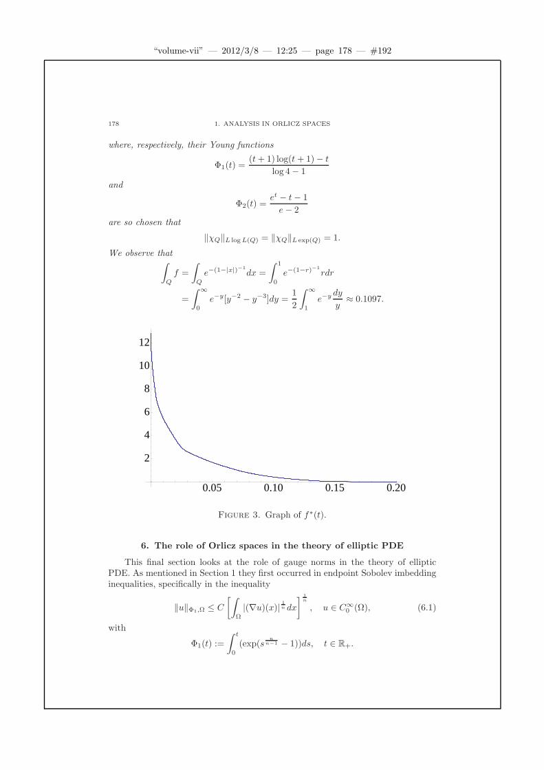
“volume-vii” — 2012/3/8 — 12:25 — page 178 — #192


where, respectively, their Young functions

Φ1(t) =(t+ 1) log(t+ 1)− t

log 4− 1

and

Φ2(t) =et − t− 1

e− 2

are so chosen that

‖χQ‖L logL(Q) = ‖χQ‖L exp(Q) = 1.

We observe that∫

Q

f =

∫

Q

e−(1−|x|)−1

dx =

∫ 1

0

e−(1−r)−1

rdr

=

∫ ∞

0

e−y[y−2 − y−3]dy =1

2

∫ ∞

1

e−y dy

y≈ 0.1097.

0.05 0.10 0.15 0.20

2

4

6

8

10

12

Figure 3. Graph of f∗(t).

6. The role of Orlicz spaces in the theory of elliptic PDE

This final section looks at the role of gauge norms in the theory of ellipticPDE. As mentioned in Section 1 they first occurred in endpoint Sobolev imbeddinginequalities, specifically in the inequality

‖u‖Φ1,Ω ≤ C

[∫

Ω

|(∇u)(x)| 1n dx

] 1n

, u ∈ C∞0 (Ω), (6.1)

with

Φ1(t) :=

∫ t

0

(exp(sn

n−1 − 1))ds, t ∈ R+.

“volume-vii” — 2012/3/8 — 12:25 — page 179 — #193

6. THE ROLE OF ORLICZ SPACES IN THE THEORY OF ELLIPTIC PDE 179

One can improve on (6.1) in two ways. Thus, in [BW], it is shown ‖ ‖Φ1,Ω

can be replaced by the larger (Lorentz) norm

[∫ |Ω|

0

u∗(t)n log−n

( |Ω|t

)dt

t

] 1n

.

Recently, an improvement on the Lebesgue norm in (6.1) was obtained, in[KP2], namely, the (smaller) functional – equivalent to a norm –

ρ(f) :=

∥∥∥∥∥t− 1

n

∫ |Ω|

t

f∗(s)s−1n ds

∥∥∥∥∥Φ2,IΩ

,

defined in terms of the Young function

Φ2(t) :=

∫ t

0

sn−1 log−n(s+ 10n)ds ≈ tn log−n(t+ 10n), t ∈ R+.

Finally, we focus on an elliptic nonlinear boundary value problem consideredin detail by J. P. Gossez in [G]. Its very statement involves a Young function. Forconcreteness, we state it in the context of R2.

Let Φ(t) =∫ t

oϕ(s)ds, t ∈ R+, be a Young function and suppose f : Ω −→ R,

where Ω is a bounded domain in R2. Find a function u = u(x, y) on Ω satisfying

− ∂

∂x

(ϕ

(∂u

∂x

))− ∂

∂y

(ϕ

(∂u

∂y

))= f in Ω

u = 0 on ∂Ω;

(6.2)

here, ϕ(−t) = −ϕ(t), t ∈ R+.To further simplify things we assume that Φ satisfies the 2 condition, namely

Φ(2t) ≤ cΦ(t) for all t greater than some t0 ∈ R+.Gossez sought a solution of (6.2) in the Orlicz–Sobolev space W 1

0LΦ(Ω), whichwe now define. To do this we require the norm of another Orlicz–Sobolev space,that of

W 1LΦ(Ω) :=

u ∈ LΦ(Ω) :

∂u

∂x,∂u

∂ybelong to LΦ(Ω)

,

whose norm is given through the equation

‖u‖21,Φ,Ω := ‖u‖2Φ,Ω +

∥∥∥∥∂u

∂x

∥∥∥∥2

Φ,Ω

+

∥∥∥∥∂u

∂y

∥∥∥∥2

Φ,Ω

; (6.3)

the partial derivatives appearing in (6.3) are the usual weak derivatives. The spaceW 1

0LΦ(Ω) is now defined to be the closure of C∞0 in W 1LΦ(Ω).

To motivate the condition to be put on the function f in (6.2) we first considerthe so-called Nemickii operator

T : u(x) −→ ϕ(u(x)).

Specifically, we study

D(T ) := u ∈ LΦ(Ω) : ϕ(u(x)) ∈ LΨ(Ω),

“volume-vii” — 2012/3/8 — 12:25 — page 180 — #194


in which Ψ is the Young function complementary to Φ. To this end, we define

EΦ(Ω) := f : Ω −→ R :

∫

Ω

Φ(k|f |) <∞ for all k > 0

and

LΦ(Ω) := f : Ω −→ R :

∫

Ω

Φ(|f |) <∞.

One has

Lemma 6.1.

EΦ ⊂ D(T ) ⊂ LΦ

In particular, T is a bounded operator from LΦ(Ω) into LΨ(Ω) if and only if Φsatisfies the 2 condition.

Proof. If u ∈ D(T ), then |u| ∈ LΦ(Ω) and ϕ(|u|) ∈ LΨ(Ω), so∞ >∫Ω|u|ϕ(|u|)

≥∫ΩΦ(|u|); that is, u ∈ LΦ(Ω).Again, we claim

Ψ(ϕ(t)) ≤ Φ(2t), t ∈ R+, (6.4)

assuming which, u ∈ EΦ(Ω) implies 2u ∈ LΦ(Ω) and, therefore,

∞ >

∫

Ω

Φ(2|u|) ≥∫

Ω

Ψ(ϕ(|u|)),

or

ϕ(u) = sgn(u)ϕ(|u|) ∈ LΨ(Ω). (6.5)

To see (6.4), observe that

Φ(2t) =

∫ 2t

0

ϕ(s)ds ≥∫ 2t

t

ϕ(s)ds

≥ tϕ(t)

= Φ(t) + Ψ(ϕ(t)), by Theorem 4.3,

> Ψ(ϕ(t)).

As for the second assertion, we first show that T bounded implies

EΦ(Ω) = LΦ(Ω) = LΦ(Ω)

and hence that Φ satisfies ∆2 condition. Indeed, suppose u ∈ LΦ(Ω) and, forn ∈ Z+, set

un(x) = (min[u+(x), n]−min[u−(x), n])χ(−n,n)(x).

Then, un ∈ EΦ(Ω) ⊂ D(T ) and

supn

‖un‖Φ,Ω 6 ‖u‖Φ,Ω <∞.

Since T is bounded

supn

‖Tun‖Ψ,Ω <∞.

“volume-vii” — 2012/3/8 — 12:25 — page 181 — #195


Holder’s inequality then yields∫

Ω

Φ(|un|) ≤∫

Ω

|un|ϕ(|un|)

≤ 2‖un‖Φ,Ω‖ϕ(|un|)‖Ψ,Ω

≤ K <∞, n = 1, 2, . . . ,

whence, by Fatou’s lemma,∫

Ω

Φ(|u|) ≤ K <∞;

that is, u ∈ LΦ(Ω), so (6.5) holds.Assume, next, Φ satisfies the 2 condition and let u vary in a bounded set in

D(T ); in particular, there exists k > 1 with∫

Ω

Φ

(2|u|k

)≤ 1

for all u in the set.Let t0 > 0 and C > 1 be such that

Φ(kt) ≤ CΦ(t), for t ≥ t0 > 0,

Then∫

Ω

Φ (2|u|) =∫

2|u|k ≥t0

Φ (2|u|) +∫

2|u|k <t0

Φ (2|u|)

≤ C

∫2|u|k ≥t0

Φ

(2|u|k

)+Φ(kt0)|Ω| ≤ C +Φ(kt0)|Ω|,

for all u in the set. Further, (6.4) yields∫

Ω

Ψ(ϕ(|u|)) ≤∫

Ω

Φ(2|u|) ≤ C +Φ(kt0)|Ω|

where, for all u in the set,

‖ϕ(u)‖Ψ,Ω ≤ max

[1,

∫

Ω

Ψ(ϕ(|u|))]≤ C +Φ(kt0)|Ω| <∞.

Remark 6.2. Suppose the Young function Φ satisfies the 2 condition andconsider u ∈ W 1

0LΦ(Ω). Such a u being in LΦ(Ω), one has, in view of Lemma 6.1,

that ϕ(u) ∈ LΨ(Ω). But, then∂ϕ(u)

∂x, say, defines a bounded linear functional on

W 10LΦ(Ω), since, for v ∈ W 1

0LΦ(Ω),∣∣∣∣∫

Ω

v∂ϕ(u)

∂x

∣∣∣∣ =∣∣∣∣∫

Ω

ϕ(u)∂v

∂x

∣∣∣∣

6 2‖ϕ(u)‖Ψ,Ω

∥∥∥∥∂v

∂x

∥∥∥∥Φ,Ω

6 2‖ϕ(u)‖Ψ,Ω ‖v‖W 10 LΦ(Ω) .

“volume-vii” — 2012/3/8 — 12:25 — page 182 — #196


This tell us it is reasonable to take f in (6.2) to be a bounded linear functional onW 1

0LΦ(Ω).It only remains to clarify the sense in which

u = 0 on ∂Ω

when u ∈W 1LΦ(Ω).We assume Φ satisfies the 2 condition and Ω is a Lipschitz domain, so, in

particular, it has the segment property, whereby there exists a locally finite opencovering, Oi, of ∂Ω and corresponding vectors, yi, such that for x ∈ ∂Ω andt ∈ (0, 1), one has x+ tyi ∈ Ω.

As proved in section 2.2 of [G], C∞(Ω) is dense inW 1LΦ(Ω). Again, in section2.3 it is shown that for the restriction mapping

γ : C∞(Ω) −→ C(∂Ω)

defined by

γ(u) := u|∂Ω,there holds

‖γ(u)‖Φ,∂Ω ≤ K‖u‖W 1LΦ(Ω), (6.6)

when u ∈ C∞(Ω). The above-mentioned density of C∞(Ω) in W 1LΦ(Ω) then en-sures that γ can be extended to all of W 1LΦ(Ω) , this extension, denoted by γ, beingcalled the trace operator, with, of course,

‖γ(u)‖Φ,∂Ω ≤ K‖u‖W 1LΦ(Ω), u ∈ W 1LΦ(Ω).

Lastly, the Proposition of section 2.3 tells us that the kernel of γ is in W 10LΦ(Ω),

so, if u ∈ C∞(Ω),

u|∂Ω ≡ 0.

We are now able to properly state

Theorem 6.3. Let Ω be a bounded Lipschitz domain in R2. Suppose ϕ : R −→R is continuous and strictly increasing, with ϕ(0) = 0 and limt−→∞ ϕ(t) = ∞.Assume,

Φ(t) :=

∫ t

0

ϕ(s)ds, t ∈ R+

satisfies the 2 condition.Then, to any bounded linear functional, f , on W 1LΦ(Ω) there corresponds a

unique u ∈ W 10LΦ(Ω) such that ϕ

(∂u

∂x

)and ϕ

(∂u

∂y

)belong to the Kothe dual,

LΨ(Ω), of LΦ(Ω) and, as distributions,

− ∂

∂xϕ

(∂u

∂x

)− ∂

∂yϕ

(∂u

∂y

)= f.

Example 6.4. The Young function Φ(t) =∫ t

0log(1 + s)ds for the Orlicz

space L logL satisfies the 2 condition, so Theorem 6.3 guarantees the uniquesolution, u, to (6.3) in any Lipschitz domain Ω, whenever T is a bounded lin-ear functional on W 1

0L logL(Ω). It is a conseuence of the imbedding theory in

“volume-vii” — 2012/3/8 — 12:25 — page 183 — #197


[KP1] that, in fact, u belongs to an Orlicz space smaller than L logL(Ω), namely

to Ln′

(logL)n′

(Ω),n′ =n

n− 1, defined through the Young function

Φ(t) =

∫ t

0

sn′−1 logn

′

(1 + s)ds, t ∈ R+.

“volume-vii” — 2012/3/8 — 12:25 — page 184 — #198

“volume-vii” — 2012/3/8 — 12:25 — page 185 — #199

Bibliography

[BS] C. Bennett and R. Sharpley, Interpolation of Operators, Pure and AppliedMathematics Vol. 129, Academic Press, Boston 1988.

[BW] H. Brezis and S. Wainger, A note on limiting cases of Sobolev embeddingsand convolution inequalities, Comm. Partial Differential Equations 5 (1980),773–789.

[FKPS] M. Francu, R. Kerman, C. Phipps and A. Sayfy, Finite element approxi-mations to rearrangements, Preprint.

[G] J. P. Gossez, Orlicz–Sobolev spaces and nonlinear elliptic boundary value prob-lems, NAFSA Spring School, Horni Bradlo, 1978, http://project.dml.cz.

[KP1] R. Kerman and L. Pick, Optimal Sobolev imbeddings, Forum Math. 18

(2006), no. 4, 535–570.[KP2] R. Kerman and L. Pick, Explicit formulas for optimal rearrangement-

invariant norms in Sobolev imbedding inequalities, Preprint.[KR] M. A. Krasnoselskii and Ya. B. Rutickii, Convex functions and Orlicz spaces,

GITTL, Moscow, 1958, english transl./ Noordhoff, Groningen, 1961.[L] W. A. J. Luxemburg, Banach function spaces, Ph.D. Thesis, Delft Institute of

technology, Assen (Netherlands), 1955.

185

“volume-vii” — 2012/3/8 — 12:25 — page 186 — #200

“volume-vii” — 2012/3/8 — 12:25 — page 187 — #201

Part 6

Topics in the Q-tensor theory of

liquid crystals

Arghir Zarnescu

“volume-vii” — 2012/3/8 — 12:25 — page 188 — #202

2000 Mathematics Subject Classification. Primary 82D30 (35A15 35B25 76A1576M30)

Key words and phrases. complex non-Newtonian fluids, liquid crystals, defects,biaxial, uniaxial, Q-tensor, Navier–Stokes, harmonic maps

Abstract. These lecture notes are intended to be a brief introduction into themathematical problems of the Q-tensor theory of liquid crystals. Emphasis isplaced on those aspects in which tensorial features are significant and on theirphysical relevance.

Acknowledgement. The author gratefully acknowledges the hospitality ofNecas Center in September 2010.

“volume-vii” — 2012/3/8 — 12:25 — page 189 — #203

Contents

Chapter 1. Mathematical modelling 1911. Some history and the main physical aspects 1911.1. Birefringence and “defect” textures 1922. The probability distribution function and the Q-tensor 1932.1. Q-tensors: beyond liquid crystals 1963. Some simple properties of Q-tensors 1963.1. Physical Q-tensors and eigenvalues constraints 1963.2. Characteristic equation and uniaxial Q-tensors 1974. A Q-tensor model: the Beris-Edwards system 1985. Defect patterns and their diverse descriptions 200

Chapter 2. Qualitative features of a stationary problem: Oseen–Frank limit 2031. Preliminaries 2042. The limiting harmonic map and the uniform convergence 2063. Biaxiality and uniaxiality 2203.1. The bulk energy density 2203.2. Analyticity and uniaxiality 227

Chapter 3. Well-posedness of a dynamical model: Q-tensors andNavier–Stokes 231

1. The dissipation and apriori estimates 2312. Weak solutions 2343. Strong solutions 238

Bibliography 243

Appendix A. Representations of Q and the biaxiality parameter β(Q) 247

Appendix B. Properties of the bulk term fB(Q) 251

189

“volume-vii” — 2012/3/8 — 12:25 — page 190 — #204

“volume-vii” — 2012/3/8 — 12:25 — page 191 — #205

CHAPTER 1

Mathematical modelling

1. Some history and the main physical aspects

The story of liquid crystals began in 1888 in the beautiful city of Prague witha discovery of the Austrian botanical physiologist Friedrich Reinitzer. During hisstudies at Charles University, Reinitzer noticed that an organic substance relatedto cholesterol “melted” into a cloudy liquid at approximately 145 C and became aclear liquid at approximately 178 C. The cloudy liquid was what is now known asa cholesteric liquid crystals.

Reinitzer asked for help from a physicist, Otto Lehmann, who was working atthat time in Aachen. They exchanged letters and samples and Lehmann becamevery interested in the newly discovered material particularly because its specificitythat was revealed by a novel (at that time) technique that Lehmann was veryinterested in, namely polarized microscopy. Under the polarized microscope, theapparently liquid substance revealed optical properties more specific to crystalsthan to a liquid. It was Lehmann who coined the “liquid crystal” name and whofought a bitter battle for the recognition of the new material. However it took untilthe early 1920s for liquid crystals to became recognized as a new, overall, phase ofmatter, with properties between liquids and solids.

Liquid crystals are “crystals that flow”. Although it sounds contradictory, thename captures the specificity of liquid crystals as phase of matter that is inter-mediate between crystalline solids and isotropic fluids, by sharing properties withboth phases. The material flows like a nearly incompressible viscous fluid and stillretains several features, especially optical, characteristic of crystals. Nowadays thematerial is mathematically modeled as a complex non-Newtonian fluid.

Liquid crystal materials are called mesogenic because of their capacity to gen-erate intermediate phases of matter, that is mesophases. There are essentially twoways of obtaining a liquid crystalline phase in a mesogenic substance:

• by changing the temperature, in which case we obtain thermotropic liquidcrystals or

• by changing the concentration of molecules in a solvent in order to obtainlyotropic liquid crystals.

It was G. Friedl who in 1922 in [Fri22] proposed the modern classification ofthe main types of liquid crystals, separating them into nematic, cholesteric andsmectic. In the rest of these notes we shall be concerned only with the simplesttype: the nematics (more precisely thermotropic nematics).

Nematic liquid crystals consist of molecules that have rod-like shape, whosethickness is much smaller than their length. Although the centres of mass of the

191

“volume-vii” — 2012/3/8 — 12:25 — page 192 — #206

192 1. MATHEMATICAL MODELLING

molecules are isotropically distributed, the direction of the molecules is, on averageover small regions in space, constant! Moreover, the rod-like molecules are locallyinvariant with respect to reflection in the plane perpendicular to the preferreddirection. This is commonly referred to as the ‘head-to-tail’ symmetry [Gen74].

The name “nematic” comes from the Greek νηµα which means “thread”. Wewill see in the next subsection a justification for this name.

1.1. Birefringence and “defect” textures. Liquid crystals are an anisotro-pic, inhomogeneous material that is optically birefringent. That is, it has (locally)two indices of refraction. Light polarized parallel to the director has a different indexof refraction (in particular it travels at a different velocity) than light polarizedperpendicular to the director. However not every direction is a direction of doublerefraction. Directions of single refraction are called “optic axis directions”. Thuslight transmitted along a path parallel to the optic axis has only a single refractiveindex. Depending on the properties of the liquid crystal material at any given pointthere can be either one or two directions of single refraction. Points where thereis a single optic axis are called “unixial” while the other ones are called “biaxial”.There can also be (rare) points where the light has the same index of refractionin any direction, and these points are called “isotropic”. This optic terminology isrelevant to the Q-tensor one in the following section.

The most common way of probing the nature of a liquid crystal material isby sending monochromatic (single wave-length) linearly polarized light through athin layer of liquid crystal material placed between two crossed polarizers. Be-cause of the birefringent nature of the sample, the incoming linearly polarized lightbecomes elliptically polarized. When this ray reaches the second polarizer, thereis now (generically) a component that can pass through, and the region appearsbright through the second polarizer. However this is not always the case. If thetransmission axis of the first polarizer is parallel to either of the two special di-rections (called the ordinary or extraordinary directions), the light is not brokenup into components, and no change in the polarization state occurs. In this case,there is no transmitted component and the region appears dark through the secondpolarizer. This property is responsible for the basic mechanism of a liquid crystaldisplay. In the simplest such display one places a source of light of a certain fre-quency under a thin layer of liquid crystals . In the absence of an exterior field onewould only see a dark state on the other side. However, switching on an electricfield the state of the molecules will be distorted so that the light will pass and onewill observe a bright state.

Up to this point, we have considered using only monochromatic light (singlewave-length). However if the liquid crystal material is illuminated by white light(all light frequencies) the wavelengths will experience some retardation and emergefrom the full-wave plate in a variety of polarization states, that appear as variouscolors.

Among the patterns observed in experiments, there exist at least two typesthat are of a particular significance. A first type refers to systems of dark, flex-ible filaments. It is these thread-like filaments that are responsible for the nameof “nematics”. As De Gennes notes in [Gen74], Ch.4 some appear to be floating

“volume-vii” — 2012/3/8 — 12:25 — page 193 — #207

2. THE PROBABILITY DISTRIBUTION FUNCTION AND THE Q-TENSOR 193

entirely the fluid, while others have both ends attached to the walls, or are en-tirely attached to the walls. De Gennes called these structures “black filaments” or“structures a fils”. F.C. Frank in [Fra58] referred to them as “disclinations” andthey are commonly referred to as “line defects”.

On the other hand it is possible to see only systems of singular points connectedby black stripes. These points are called “structures a noyaux” by De Gennesin [Gen74] and they (together with the patterns around them) are referred to as“schlieren” textures in the German literature. They are commonly referred to as“point defects”.

One can naturally ask that if one has 1D defects (line defects) as well as 0Ddefects (point defects) why not 2D defects? In [Gen74], Ch.4 De Gennes providesa crude explanation for the lack of defects, arguing that they are “energeticallyexpensive” hence they cannot appear in energy minimizers. In this explanationDe Gennes uses the Oseen–Frank director description of nematics (see the nextsection). However, when using his own Q-tensor description of the nematics heargues against the existence of wall defects based on what are essentially symmetryconsiderations [Gen72].

Defect patterns are an essential characteristic of nematic liquid crystals andthus they are a benchmark test for determining the relevance of a nematic liquidcrystal model. A good model should be able to describe these patterns and predicttheir appearance. In Section 5 we will see to what extent the available theories arecapable of describing these patterns.

2. The probability distribution function and the Q-tensor

The main physical characteristics of nematics (locally preferred directions and‘head-to-tail’ symmetry) can be modelled by assigning to each material point x, inthe region Ω occupied by the liquid crystal, a probability measure µ(x, ·) : L(S2) →[0, 1] for describing the orientation of the molecules, where L(S2) denotes the familyof Lebesgue measurable sets on the unit sphere. Thus µ(x,A) gives the probabilitythat the molecules with centre of mass in a very small neighbourhood of the pointx ∈ Ω are pointing in a direction contained in A ⊂ S2.

Nematic liquid crystals are locally invariant with respect to reflection in theplane perpendicular to the preferred direction. This is commonly referred to as the‘head-to-tail’ symmetry, see [Gen74]. This means that µ(x,A) = µ(x,−A), for allx ∈ Ω, A ⊂ L(S2). Note that because of this symmetry the first moment of theprobability measure vanishes:

〈p〉 def=

∫

S2

p dµ(p) =1

2

[∫

S2

p dµ(p) +

∫

S2

−p dµ(−p)]= 0.

The first nontrivial information on µ comes from the tensor of second moments:

Mijdef=

∫

S2

pipj dµ(p), i, j = 1, 2, 3

We have M =MT and trM =∫S2dµ(p) = 1. Let e be a unit vector. Then

e ·Me =

∫

S2

(e · p)2 dµ(p) = 〈cos2(θ)〉

“volume-vii” — 2012/3/8 — 12:25 — page 194 — #208


where θ is the angle between p and e.If the orientation of the molecules is equally distributed in all directions we

say that the distribution is isotropic and then µ = µ0 where dµ0(p) =14πdA. The

corresponding second moment tensor is

M0def=

1

4π

∫

S2

p⊗ p dA =1

3Id

(since∫S2p1p2 dµ(p) = 0,

∫S2p21 dµ(p) =

∫S2p22 dµ(p) =

∫S2p23 dµ(p) and trM0 = 1).

The de Gennes order-parameter tensor Q is then defined as

Qdef= M −M0 =

∫

S2

(p⊗ p− 1

3Id

)dµ(p) (2.1)

and measures the deviation of the second moment tensor from its isotropic value.Since Q is symmetric and trQ = 0, Q has, by the spectral theorem, the repre-

sentation:

Q = λ1e1 ⊗ e1 + λ2e2 ⊗ e2 − (λ1 + λ2)e3 ⊗ e3 (2.2)

where e1, e2, e3 is an orthonormal basis of eigenvectors of Q with the correspondingeigenvalues λ1, λ2 and λ3 = −(λ1 + λ2).

When two of the eigenvalues are equal (and non-zero) the order parameter Qis called uniaxial, otherwise being biaxial. It is an easy exercise, using the spectral

representation and the fact that Id =∑3

i=1 ei ⊗ ei to show that any uniaxialQ-tensor can be represented in the form

Q = s

(n⊗ n− 1

3Id

)

with n ∈ S2 and for some scalar s ∈ R.

The Q = 0 tensor is called the isotropic state. This kind of classification ofnematics comes from optics, and we saw in the previous section the optical relevanceof the terms “biaxial” and “uniaxial”. From now on we will refer to symmetric,traceless, d x d-matrices (d = 2 or d = 3) as Q-tensors. More about the physicalinterpretation and relevance of the Q-tensors will be mentioned in Section 3.1 (seefor further details [MN04], [Maj10]).

Equilibrium configurations of liquid crystals are obtained, for instance, as en-ergy minimizers, subject to suitable boundary conditions. The simplest commonlyused energy functional is

FLG[Q] =

∫

Ω

L2

3∑

i,j,k=1

Qij,kQij,k −a

2trQ2 − b

3trQ3 +

c

4

(trQ2

)2 dx (2.3)

where a, b, c are temperature and material dependent constants and L > 0 is theelastic constant. In the physically significant limit L → 0 (and for appropriateboundary conditions, see for details Chapter 2) we have that the energy minimizersare suitably approximated by minimizers of the corresponding ‘Oseen–Frank energyfunctional’

FOF [Q] =

∫

Ω

3∑

i,j,k=1

Qij,kQij,k dx

“volume-vii” — 2012/3/8 — 12:25 — page 195 — #209

2. THE PROBABILITY DISTRIBUTION FUNCTION AND THE Q-TENSOR 195

in the restricted class of Q ∈ W 1,2( where W 1,2 (Ω;S0) is the Sobolev space ofsquare-integrable Q-tensors with square-integrable first derivatives [Eva98]), withQ uniaxial a.e., so that

Q = s

(n⊗ n− 1

3Id

)(2.4)

with s ∈ R (an explicit fixed constant depending on a, b and c but independent ofx ∈ Ω) and n(x) ∈ S2 a.e. x ∈ Ω.

This convergence, as L→ 0, was studied initially in [MZ10] and further refinedin [NZ]. If we restrict ourselves to working with tensors Q that admit a representa-tion as in (2.4), for a fixed s independent of x ∈ Ω we refer to this as the constrainedDe Gennes theory.

The reason for referring to (2) as an “Oseen–Frank functional” has to do withthe relations that the functional has with the celebrated Oseen–Frank theory ofnematics. The theory was proposed in the 1950s, in [Fra58]. The Oseen–Franktheory does not use matrices as in (2.4) but rather unit vectors, hence the materialis modeled through a vector-field n : Ω ⊂ Rd → Sd−1, d = 2, 3. The theoryhas the deficit of ignoring the physical head-to-tail symmetry of the material buthas the advantage of being simpler as it is more convenient to manipulate vector-valued functions, rather than matrix-valued ones. In particular the theory usesmathematical objects with just two degrees of freedom, namely vectors n ∈ S

2,unlike the theory of De Gennes that uses objects with five degrees of freedom(Q-tensors).

If one formally replaces the formula (2.4) into (2.3) (with s a fixed constant,independent of x ∈ Ω) one obtains:

FLG[Q] =

∫

Ω

L

2

3∑

i,j,k=1

Qij,kQij,k dx+C = FOF [n]+C = 2s2∫

Ω

3∑

i,j,k=1

ni,kni,k dx+C

(where C is an explicitly computable constant) so apparently nothing is lost, at en-ergy level, when passing from the matrix representation to the vector representationform of the Oseen–Frank theory. However, in order to derive the equality above weimplicitly assumed that the vector-valued functions n are as smooth as the matrix-valued functions Q. This might not always be the case and indeed it turns out thatthere can be significant differences between the classical Oseen–Frank theory andthe constrained De Gennes theory. These differences are analyzed in [BZ].

An important deficit of the Oseen–Frank theory has to do with its incapacityof predicting higher dimensional defects, as we will discuss in Section 5. The theorycan predict only point-like defects, but not the more complicated line or wall defects.

Returning to the Q-tensors and taking into account how they are obtained,namely the definition (2.1) of the tensor Q and assuming that Q is uniaxial so ithas a representation as in (2.4) we have that

Qn · n =2

3s = 〈(p · n)2 − 1

3〉 = 〈cos2 θ − 1

3〉

where θ is the angle between p and n. We have s = 32 〈cos2 θ − 1

3 〉 and so we must

necessarily have − 12 ≤ s ≤ 1 with s = 1 when we have perfect ordering parallel to

n, s = − 12 when all molecules are perpendicular to n and s = 0 iff Q = 0 (which

“volume-vii” — 2012/3/8 — 12:25 — page 196 — #210


occurs if µ is isotropic). Thus s is a measure of order and is called the scalar orderparameter associated to the tensor Q. In the physical literature it is often assumedthat s is constant almost everywhere. For experimental determinations of s see forinstance [CEG+06]. Various experimental methods for the determination of s arealso presented in the older paper of A. Rapini, [Rap73], pp. 362− 364.

Motivated by this representation, and in an attempt to overcome the limitationsof the Oseen–Frank theory, J.L. Ericksen proposed in the 1990s, in [Eri90] a moreelaborate theory than that of Oseen–Frank. His theory describes nematics throughpairs (s, n) : Ω → [− 1

2 , 1] × S2 so that n describes the orientation of the directorand s is the degree of order. If s = 0 then n needs not be defined. The nematicsin Ericksen’s theory are thus described as objects with three degrees of freedom,intermediary between the theory of Oseen–Frank that uses only two and that of DeGennes that uses five degrees of freedom. Ericksen theory proposes an alternativedefinition of defects, and manages to predict the more complicated line or walldefects, but however it does not capture properly the head-to-tail symmetry of themolecules.

We have thus three major theories attempting to describe nematics: Oseen–Frank, Ericksen and Landau-de Gennes. Each theory uses different mathematicalobjects to describe the same physical reality and, as we will see in Section 5, eachproposes different explanations of the defect patterns.

2.1. Q-tensors: beyond liquid crystals. The type of local orientationalorder that exists in nematics is by no means an isolated phenomena in nature.Liquid crystal ordering is found in various different systems, including polymers,amphiphile solutions, elastomers, carbon nanotubes and biological systems (forexample, the liquid crystal states of DNA). Thus the Q-tensor description shouldbe suitable for the treatment of such complex systems. More on the nematic defectsas they appear in carbon nanotubes can be found in [ZK08].

3. Some simple properties of Q-tensors

3.1. Physical Q-tensors and eigenvalues constraints. Let us recall, (2.1),that a Q-tensor was defined as a normalized second-order moment of a probabilitymeasure µ. One can easily see that there can be different probability measures µ0

and µ1 such that the corresponding Q-tensors are the same. For instance we can

take µ0 to be the uniform probability measure as before and µ1 = 16

∑3i=[δei +δ−ei ]

where δei denotes the Dirac delta measure concentrated at ei, with e1, e2, e3 anorthonormal basis in R3. Then the corresponding Q-tensors are the same, namelythe isotropic Q-tensors.

On the other hand the representation formula (2.1) imposes some restrictionson the eigenvalues of Q. Recalling the spectral representation of Q,(2.2), and theprobabilistic definition of Q, (2.1), we have:

λi = (Qei) · ei =∫

S2

(p · ei)2dµ(p)−1

3

“volume-vii” — 2012/3/8 — 12:25 — page 197 — #211

3. SOME SIMPLE PROPERTIES OF Q-TENSORS 197

Since µ is a probability measure we have 0 ≤∫S2(p · ei)2 dµ(p) ≤ 1 and thus the

last relation implies a constraint on the eigenvalues λi, i = 1, 2, 3 of Q, namely:

−1

3≤ λi ≤

2

3, i = 1, 2, 3 (3.1)

Further discussions on the physical relevance and constraints on the Q-tensorsare available in [Maj10]. A way of enforcing, at a variational level, the eigenvaluesof Q-tensors to stay within the physical region delimitated in (3.1) is by using apotential that blows-up logarithmically when the eigenvalues approach the limitvalues [BM10].

Let us denote by |Q| the Frobenius norm of a Q-tensor, namely:

|Q| def=√tr(QQt) =

√tr(Q2) =

√√√√3∑

i,j=1

QijQij =√λ21 + λ22 + λ23

For the physical Q-tensors, the restrictions (3.1) impose a bound on the size of|Q|. On the other hand a bound on the size of |Q| imposes restrictions only on thesize of λ21+λ

22+λ

23 and thus it might not be enough to obtain the more complicated

constraints (3.1).

3.2. Characteristic equation and uniaxial Q-tensors. Using the charac-teristic equation and the Cayley-Hamilton theorem one easily obtains:

Proposition 3.1. For any Q-tensor we have:

(i)

Q3 − 1

2|Q|Q− detQ · Id = 0,

(ii)

tr(Q3) = 3 det(Q),

(iii)

tr(Q4) =1

2|Q|4.

Let us recall that a Q-tensor is uniaxial if it has two equal eigenvalues. We caneasily characterize such Q-tensors:

Proposition 3.2. A Q-tensor is uniaxial if and only if

|Q|6 = 54(detQ)2 = 6 tr(Q3) (3.2)

Proof. The characteristic equation of Q is:

det(Q− λId) = −λ3 + tr(Q)λ2︸︷︷︸=0

−λ tr(cof Q) + detQ.

But 2 tr(cof Q) = 2(λ2λ3+λ3λ1+λ1λ2) = (λ1 + λ2 + λ3︸︷︷︸=tr(Q)=0

)2−(λ21+λ22+λ

23) = −|Q|2.

Hence the characteristic equation becomes:

λ3 − 1

2|Q|2λ− detQ = 0

“volume-vii” — 2012/3/8 — 12:25 — page 198 — #212


and the condition that λ3−pλ+q = 0 has two equal eigenvalues becomes: p ≥ 0 and4p3 = 27q2, which gives the first equality in the conclusion. The second equality iseasily obtained by observing that we just need to verify it on diagonal matrices asfor any Q there exists a R ∈ O(3) such that RQRt is diagonal and replacing Q byRQRt does not change detQ nor tr(Q3).

Remark 3.3. An alternative proof of the previous proposition, without usingfacts about third-order equations, is provided in Lemma 0.5

Let us recall that a uniaxial Q-tensor can be written as Q = s(n⊗ n− 1

3Id),

where s ∈ R and n ∈ S2. If we fix the s to be a given non-zero constant, say s+,we obtain the class of constrained Q-tensors:

S∗def= s+

(n⊗ n− 1

3Id

), n ∈ S

2 (3.3)

One can easily show (see also [NZ]):

Lemma 3.4. A Q-tensor belongs to S∗ if and only if one of the following holds:

(i) tr(Q2) =2s2+3 and tr(Q3) =

2s3+9 . (ii) The minimal polynomial of Q is λ2− s+

3 λ =29s

2+.

4. A Q-tensor model: the Beris-Edwards system

The most complete descriptions of liquid crystals regard them as a complexnon-Newtonian fluid. There exist various specific models that all use the Q-tensordescription and a comparative discussion of the main models is available for instancein [SMV04].

In these notes we use a model proposed by Beris and Edwards [BE94], that onecan find in the physics literature for instance in [DOY], [TDY03] (however in the lasttwo references the fluid is assumed compressible (for computational purposes only)and with variable density). An important feature of this model is that if one assumessmooth solutions and one formally takes Q(x) = s+(n(x) ⊗ n(x) − 1

3Id), with s+a constant (depending on the parameters of the system, see for instance [MZ10])and n : Rd → Sd−1 smooth, then the equations reduce (see [DOY]) to the generallyaccepted equations of Ericksen, Leslie and Parodi [Les68]. The system is relatedstructurally to other models of complex fluids coupling a transport equation with aforced Navier-Stokes system [CFTZ07], [CM01], [LM00], [LZZ08],[Lin91], [Mas08],[Sch09]. In our case the Navier-Stokes equations are coupled with a parabolic typesystem, but we also have two more derivatives (than in the previously mentionedmodels) in the forcing term of the Navier-Stokes equations. The Ericksen-Leslie-Parodi system describing nematic liquid crystals, whose structure is closer to oursystem (but that has one less derivative in the forcing term of the Navier-Stokesequations) was studied in [LL95], [LL00], [LLW10].

In the following we use a partial Einstein summation convention, that is weassume summation over repeated indices. We consider the equations as describedin [DOY], [TDY03] but assume that the fluid has constant density in time and isincompressible.

“volume-vii” — 2012/3/8 — 12:25 — page 199 — #213

4. A Q-TENSOR MODEL: THE BERIS-EDWARDS SYSTEM 199

We denote

S(∇u,Q)def= (ξD+Ω)(Q+

1

dId)+(Q+

1

dId)(ξD−Ω)−2ξ(Q+

1

dId) tr(Q∇u) (4.1)

where Ddef= 1

2 (∇u+ (∇u)t) and Ωdef= 1

2 (∇u− (∇u)t) are the symmetric partand the antisymmetric part, respectively, of the velocity gradient tensor ∇u. Theconstant d is the dimension of the space and Q is a function on Rd that is Q-tensor valued. The term S(∇u,Q) appears in the equation of motion of the order-parameter, Q, and describes how the flow gradient rotates and stretches the order-parameter. The constant ξ depends on the molecular details of a given liquid crystaland measures the ratio between the tumbling and the aligning effect that a shearflow would exert over the liquid crystal directors.

We also denote:

Hdef= −aQ+ b[Q2 − tr(Q2)

dId]− cQ tr(Q2) + L∆Q (4.2)

where L > 0.With the notations above we have the coupled system:

(∂t + u · ∇)Q − S(∇u,Q) = ΓH(∂t + uβ∂β)uα = ν∂2βuα + ∂αp+ ∂βταβ + ∂βσαβ∂γuγ = 0

(4.3)

where Γ > 0, ν > 0 and we have the symmetric part of the additional stress tensor:

ταβdef= −ξ

(Qαγ +

δαγd

)Hγβ − ξHαγ

(Qγβ +

δγβd

)+ 2ξ

(Qαβ +

δαβd

)QγδHγδ

− L∂βQγδ∂αQγδ

and an antisymmetric part:

σαβdef= QαγHγβ −HαγQγβ

In the rest of the notes we restrict ourselves to the case ξ = 0. This means thatthe molecules are such that they only tumble in a shear flow, but are not alignedby such a flow. In this case the system (4.3) reduces to:

(∂t + uγ · ∂γ)Qαβ − ΩαγQγβ +QαγΩγβ

= Γ

(L∆Qαβ − aQαβ + b[QαγQγβ − δαβ

dtr(Q2)]− cQαβ tr(Q

2)

)

(∂t + uβ∂β)uα = ν∆uα + ∂αp− L∂β (∂αQζδ∂βQζδ)

+ L∂β (Qαγ∆Qγβ −∆QαγQγβ)

∂γuγ = 0

(4.4)in Rd, d = 2, 3 where we use the summation convention over repeated indices and

note that we have that the matrices −aQ + b[Q2 − tr(Q2)d Id] − cQ tr(Q2) and Q

commute, hence QH −HQ = L(Q∆Q−∆QQ).We also need to assume from now on that

c > 0 (4.5)

“volume-vii” — 2012/3/8 — 12:25 — page 200 — #214


This assumption is necessary from a modelling point of view (see [Maj10],[MZ10] )so that the energy F is bounded from below, and is also necessary for having globalsolutions (see Proposition 1.2 and its proof).

5. Defect patterns and their diverse descriptions

An important test of any theory attempting to describe nematics concerns thepredictive capacities of the theory with regard to defect patterns. The simplesttheory, the Oseen–Frank theory uses unit-vectors to describe nematics, that is thenematics are modelled as vectors fields n : Ω ⊂ Rd → Sd−1. In this theory defectsare simply discontinuities of vectors and this is one reason why his theory has beenextremely successful with mathematicians interested in regularity problems.

In Oseen–Frank theory equilibrium configurations are obtained as energy min-imizers of the energy functional that we saw in a previous section, namely:

FOF =

∫

Ω

|∇n(x)|2 dx (5.1)

where the minimization is done the space

W 1,2ϕ (Ω, Sd−1)

def= n : Ω → R

d; n(x) ∈ Sd−1 a.e. x ∈ Ω, and n(x) = ϕ(x), for a.e. x ∈ ∂Ω

(5.2)

with ϕ : ∂Ω → Sd−1 an imposed boundary condition.The minimizers satisfy the Euler–Lagrange system of equations:

∆ni = −ni|∇n|2, i = 1, . . . , d (5.3)

|n(x)| = 1 a.e. x ∈ Ω (5.4)

The above equations are known as the harmonic map equations and they havebeen widely studied, particularly from the point of view of regularity and partialregularity, a recent monograph in the area being [LW08].

One of the important limitations of the Oseen–Frank theory is that it onlyrecognizes points defects, as defects with finite energy. While line and wall defectsmight be interpreted in this framework, they always have infinite energy.

In the more complex Ericksen theory the equilibrium configurations are ob-tained as minimizers of an energy functional that in its simplest form is:

FE(s, n) =

∫

Ω

k|∇s(x)|2 + s(x)|∇n(x)|2 + w0(s(x)) dx (5.5)

where k > 0 is a constant and the minimization is in the space

A def= (n, s) : Ω → S

d−1 × R, (s · n, s) ∈ H1, and s = s0, sn = s0n0 on ∂Ωwhere (s0, n0) : ∂Ω → [− 1

2 , 1]× Sd−1 are imposed boundary conditions.The Ericksen model was studied in several papers, mainly related to Fanghua

Lin, see for instance [LP94]. In Ericksen theory the defects are regarded as thezero set of s, that is the points where the degree of order is zero, i.e. there is nopreferred direction of the molecules. This proposes a compelling explanation forthe defects and the energy minimizers in this theory are found indeed to have both

“volume-vii” — 2012/3/8 — 12:25 — page 201 — #215

5. DEFECT PATTERNS AND THEIR DIVERSE DESCRIPTIONS 201

line and wall defects, of finite energy, unlike in the Oseen–Frank model. However,the actual experimental techniques do not allow to probe close enough to the coreof a defect to experimentally check the relevance of this proposed explanation fordefects.

On the other hand in the Q-tensor theory of De Gennes defects seem to have avery different nature. The problem of defects in the framework of De Gennes theoryhas not attracted much attention in the physics literature, perhaps because theOseen–Frank theory, despite its limitations and thanks to its relative simplicity, hasproved to be very attractive for describing defects, particularly from a topologicalpoint of view. Indeed, in fact one can talk about line and wall defects even inthe framework of the Oseen–Frank theory provided that one is willing to allowfor regions of infinite energy. The overall perspective in the physics literature isthat if one is willing to provide a substitute for these infinite energy regions, thatare the core of the defects, then the Oseen–Frank theory works reasonably welloutside the cores. Indeed, it is in these defect regions of infinite energy where thetheory of De Gennes proves its utility by providing finite energy, together with apossibly different structure for the core of the defects. Thus physicists often adoptan ambiguous position by using the simpler Oseen–Frank theory outside defectsand substituting the more complex De Gennes energy near the core of the defects.The simple variational model of De Gennes allows, in some sense, for a justificationof this perspective, see next chapter and [MZ10].

However if one attempts a definition of defects intrinsic to the Q-tensor theory,it seems that defects have quite a different nature, in this theory, when comparedto the other two theories. In his relatively unknown paper [Gen72] in the 1970, DeGennes proposes to describe defects essentially as discontinuities of eigenvectors.This definition is in some sense misleading and it should be interpreted in the sensethat one has a point of discontinuity x0 for the eigenvectors of the matrix Q(x)if it is not possible to find some continuous functions on a neighbourhood of x0,say ei(x), i = 1, 2, 3 so that Q(x)ei(x) = λi(x)ei(x), i = 1, 2, 3 (for some λi(x))and (ei(x), ej(x)) = δij , i, j = 1, 2, 3). An example is provided by the functionQ : [−1, 1]3 → S0 (where S0 denotes the set of traceless and symmetric 3 x 3matrices),

Q(x, y, z) =

1 + x y 0y 1− x 00 0 −2

For x = 0 and (y, z) ∈ [−1, 1]2 the basis of eigenvectors is made of

1√21√2

0

,

1√2

− 1√2

0

and

001

. For y = 0 and (x, y) ∈ [−1, 1] the basis of eigenvectors

is made of

100

,

010

and

001

. Thus the line 0 × 0 × [−1, 1] is a

“volume-vii” — 2012/3/8 — 12:25 — page 202 — #216


line of discontinuity of eigenvectors. Numerical computations, [SKH95] show thata situation as described above actually appears in the equilibrium solutions.

From a mathematical point of view an interesting (and specific) feature ofmatrix-valued functions is that even if they are real analytic it is still possible forthem to have discontinuities of eigenvectors in the sense mentioned above. Thesediscontinuities are related to the number of distinct eigenvalues. Thus, if one isin a biaxial region, or in a uniaxial region (i.e. the number of distinct eigenvaluesis constant) then one can choose the eigenvectors to be as smooth as Q(see forinstance [Kat76],[Nom73]). Thus the discontinuities of eigenvectors can only occurat the biaxial-uniaxial, uniaxial-isotropic or biaxial-isotropic interfaces. Howeverthe presence of such an interface is just a necessary criterion for the existence of adiscontinuity of eigenvectors. A simple criterion for checking the presence of such

an interface can be provided by the “ biaxiality coefficient” β(Q) = 1 − 6(trQ3)

2

(trQ2)3

that is used in the physics literature to provide a measure of “how far a matrixis from being uniaxial”, and this is motivated by the fact that β(Q) ∈ [0, 1] withβ(Q) = 0 if and only if Q = 0 or Q is uniaxial, see Appendix A.

No necessary and sufficient analytic criterion seems to be known and devisingthis can be an interesting problem. Having a sufficiently simple analytic criterionfor detecting discontinuities of eigenvectors would be of paramount importance inattempting to study the evolution in time of these defects.

Particularly relevant to this problem could be the examples of eigenvector dis-continuities that were constructed in [Lin96].

“volume-vii” — 2012/3/8 — 12:25 — page 203 — #217

CHAPTER 2

Qualitative features of a stationary problem:

Oseen–Frank limit

Liquid crystals are a complex non-Newtonian fluid and the equations that areneeded to describe it are quite complicated (as we saw in the previous sections). Inthis chapter we restrict ourselves to physical situations in which the effect of the flowis negligible and aim to obtain qualitative features of equilibrium solutions, ignoringthe effect of the flow. This is done by considering global energy minimizers of asuitable energy functional.

The Landau–De Gennes energy functional, FLG, is a nonlinear integral func-tional of Q and its spatial derivatives. Physical symmetries impose certain restric-tions on the form of the energy functional, as noted in [Bal06]. In these notes wework with the simplest form of FLG (see also [MN04]) with Dirichlet boundaryconditions, Qb (refer to (1.4) next section, for a precise description), on three-dimensional domains Ω ⊂ R3 that are simply-connected. We take FLG to be[PWS75]

FLG[Q] =

∫

Ω

L

2|∇Q|2(x) + fB(Q(x)) dx (0.1)

where fB is the bulk energy density that accounts for bulk effects,

|∇Q|2 =

3∑

i,j,k=1

Qij,kQij,k

is the elastic energy density that penalizes spatial inhomogeneities and L > 0 is amaterial-dependent elastic constant. We take fB to be a quartic polynomial in theQ-tensor components, since this is the simplest form of fB that allows for multiplelocal minima and a first-order nematic-isotropic phase transition [Gen74, Vir94].This form of fB has been widely-used in the literature and is defined as follows

fB(Q) =α(T − T ∗)

2tr(Q2)− b

3tr(Q3)+c

4

(trQ2

)2

where α, b, c ∈ R are material-dependent positive constants, T is the absolute tem-perature and T ∗ is a characteristic liquid crystal temperature. We work in thelow-temperature regime T < T ∗ for which α(T − T ∗) < 0. Keeping this in mind,we recast the bulk energy density as follows:

fB(Q) = −a2

2tr(Q2)− b2

3tr(Q3)+c2

4

(trQ2

)2, (0.2)

203

“volume-vii” — 2012/3/8 — 12:25 — page 204 — #218

204 2. QUALITATIVE FEATURES OF A STATIONARY PROBLEM: OSEEN–FRANK LIMIT

where a2, b2, c2 ∈ R+ are material-dependent and temperature-dependent non-zeroconstants. The equilibrium configurations (the physically observable configura-tions) then correspond to minimizers of FLG, subject to the imposed boundaryconditions.

In Section 2, we study the limit of vanishing elastic constant L → 0 for globalminimizers, Q(L), of FLG. This study is in the spirit of the asymptotics for minimiz-ers of Ginzburg-Landau functionals for superconductors [BBH93]. The limit L→ 0is a physically relevant limit since the elastic constant L is typically very smallafter a suitable non-dimensionalization of the system. ForMBBA for instance (see[PWS75]) the elastic constant L, is of order 10−11 J m−1, and the material coeffi-cients A, B, C are of order k = 104 J m−3 . Since the typical size d of the liquidcrystalline system is of order 10−6m, after non-dimensionalization we obtain thaton a domain of size 1 we have L = L

kd2 ∼ 10−3, A, B, C ∼ 1.

We define a limiting harmonic map Q(0) as follows

Q(0) = s+

(n(0) ⊗ n(0) − 1

3Id

)

where s+ is defined in (1.3), n(0) is a minimizer of the Oseen–Frank energy, FOF ,defined as:

FOF [n] =

∫

Ω

ni,k(x)ni,k(x) dx,

subject to the fixed boundary condition n = nb ∈ C∞(∂Ω, S2) and Qb and nb arerelated as in (1.4). Then we can relatively easy show that there exists a sequence

of global minimizersQ(Lk)

such that Q(Lk) Lk→0+−→ Q(0) strongly in the Sobolev

space W 1,2. The sequenceQ(Lk)

converges uniformly to Q(0) as Lk → 0, in the

interior of Ω, away from the (possible) singularities of Q(0).These results show that the predictions of the Oseen–Frank theory (described

by the limiting map Q(0)) and the Landau–De Gennes theory agree away from thesingularities of Q(0). The presentation in this chapter follows [MZ10].

1. Preliminaries

We take our domain, Ω ⊂ R3, to be bounded and simply-connected with smooth

boundary, ∂Ω. Let S0 ⊂ M3×3 denote the space of Q-tensors, i.e.

S0def=Q ∈ M

3×3;Qij = Qji, Qii = 0

where we have used the Einstein summation convention; the Einstein conventionwill be assumed in the rest of the paper. The corresponding matrix norm is definedto be

|Q| def=√trQ2 =

√QijQij .

As stated in the introduction, we take the bulk energy density term to be

fB(Q) = −a2

2tr(Q2)− b2

3tr(Q3)+c2

4

(tr(Q2)

)2

where a2, b2, c2 ∈ R+ are material-dependent and temperature-dependent non-zeroconstants. One can readily verify that fB is bounded from below, and we define a

“volume-vii” — 2012/3/8 — 12:25 — page 205 — #219

1. PRELIMINARIES 205

non-negative bulk energy density, fB, that differs from fB by an additive constantas follows:

fB(Q) = fB(Q)− minQ∈S0

fB (Q) . (1.1)

It is clear that fB(Q) ≥ 0 for all Q ∈ S0 and the set of minimizers of fB coincides

with the set of minimizers for fB. In Proposition 0.1, we show that the function fBattains its minimum on the set of uniaxial Q-tensors with constant order parameters+ as shown below

fB(Q) = 0 ⇔ Q ∈ Qmin where

Qmin =

Q ∈ S0, Q = s+

(n⊗ n− 1

3Id

), n ∈ S

2

(1.2)

with

s+ =b2 +

√b4 + 24a2c2

4c2. (1.3)

We work with Dirichlet boundary conditions, referred to as strong anchoringin the liquid crystal literature [Gen74]. The boundary condition Qb(x) ∈ Qmin issmooth and is given by

Qb = s+

(nb ⊗ nb −

1

3Id

), nb ∈ C∞ (∂Ω;S2

). (1.4)

We define our admissible space to be

AQ =Q ∈ W 1,2 (Ω;S0) ;Q = Qb on ∂Ω, with Qb as in (1.4)

, (1.5)

The correspondingW 1,2-norm is given by ‖Q‖W 1,2(Ω) =(∫

Ω |Q|2 + |∇Q|2dx) 1

2 .

In addition to the W 1,2-norm, we also use the L∞-norm in this paper, defined tobe ‖Q‖L∞(Ω) = ess supx∈Ω|Q(x)| .

We study global minimizers of a modified Landau–De Gennes energy functional,FLG, in the admissible space AQ. The functional FLG differs from FLG in (0.1) byan additive constant and is defined to be

FLG[Q] =

∫

Ω

L

2Qij,k(x)Qij,k(x) + fB(Q(x)) dx. (1.6)

For a fixed L > 0, let Q(L) denote a global minimizer of FLG in the admissible class,AQ. The existence of Q(L) is immediate from the direct methods in the calculus

of variations [Eva98]. The bulk energy density, fB, is bounded from below, the

energy density is convex in ∇Q and therefore, FLG is weakly sequentially lowersemi-continuous. Moreover, it is clear that FLG and FLG have the same set ofglobal minimizers for a fixed set of material-dependent and temperature-dependentconstants

a2, b2, c2, L

.

The global minimizer Q(L) is a weak solution of the corresponding Euler-Lagrange equations [BM10]

L∆Qij = −a2Qij − b2(QikQkj −

δij3

tr(Q2)

)+ c2Qij tr(Q

2) i, j = 1, 2, 3. (1.7)

where the term b2δij3 tr(Q2) is a Lagrange multiplier that enforces the tracelessness

constraint. It follows from standard arguments in elliptic regularity that Q(L) is

“volume-vii” — 2012/3/8 — 12:25 — page 206 — #220


actually a classical solution of (1.7) and Q(L) is smooth and real analytic (see also[MZ10]).

Finally, we introduce a “limiting uniaxial harmonic map” Q(0) : Ω → Qmin;Q(0) is defined to be a global minimizer (not necessarily unique) of FLG in therestricted class, AQ ∩ Q : Ω → S0, Q(x) ∈ Qmin a.e.x ∈ Ω. Then Q(0) isnecessarily of the form

Q(0) = s+

(n(0) ⊗ n(0) − 1

3Id

), (1.8)

where n(0) is a global minimizer of FOF (see [BZ]),∫

Ω

|∇n0(x)|2 dx = minn∈An

∫

Ω

|∇n(x)|2 dx (1.9)

in the admissible class An =n ∈ W 1,2

(Ω;S2

); n = nb on ∂Ω

and nb and Qb are

related as in (1.4). This “limiting harmonic” map Q(0) is therefore obtained froman energy minimizer, n0, (not necessarily unique) within the Oseen–Frank theoryfor uniaxial nematic liquid crystals with constant order parameter (for more resultsabout the relation between n(0) and Q(0) see [BZ]). It follows from standard resultsin harmonic maps [Vir94] that Q(0) has at most a finite number of isolated pointsingularities (points where n(0) has singularities). In the following sections we willelaborate on the relation between Q(L) and Q(0).

2. The limiting harmonic map and the uniform convergence

We first obtain apriori L∞ bounds, independent of L.

Proposition 2.1. Let Ω ⊂ R3 be a bounded and simply-connected open setwith smooth boundary. Let Q(L) be a global minimizer of FLG, (1.6), in the space(1.5). Then

‖Q(L)‖L∞(Ω) ≤√

2

3s+ (2.1)

where s+ is defined in (1.3).

Proof. The proof proceeds by contradiction. In the following we drop thesuperscript L for convenience. We assume that there exists a point x∗ ∈ Ω where

|Q| attains its maximum and |Q(x∗)| >√

23s+. On ∂Ω, |Q| =

√23s+ by our choice

of the boundary condition Qb (note that if Q ∈ Qmin then |Q| =√

23s+). If Q

is a global minimizer of FLG then Q is a classical solution (see Section 3.2 forregularity) of the Euler-Lagrange equations

L∆Qij = −a2Qij − b2(QipQpj −

1

3trQ2δij

)+ c2

(trQ2

)Qij . (2.2)

Since the function |Q|2 : Ω → R must attain its maximum at x∗ ∈ Ω, wenecessarily have that

∆

(1

2|Q|2

)(x∗) ≤ 0 (2.3)

“volume-vii” — 2012/3/8 — 12:25 — page 207 — #221

2. THE LIMITING HARMONIC MAP AND THE UNIFORM CONVERGENCE 207

We multiply both sides of (2.2) by Qij and obtain

L ∆

(1

2|Q|2

)= −a2 trQ2 − b2 trQ3 + c2

(trQ2

)2+ L|∇Q|2. (2.4)

We note that

−a2 tr(Q2)− b2 tr(Q3) + c2(tr(Q2)

)2 ≥ f(|Q|) (2.5)

where

f(|Q|) = −a2|Q|2 − b2√6|Q|3 + c2|Q|4, (2.6)

since tr(Q3) ≤ |Q|3√6

(see Lemma 0.5 in the Appendix). One can readily verify that

f(|Q|) > 0 for |Q| >√

2

3s+ (2.7)

which together with (2.4) and (2.5) imply that

∆

(1

2|Q|2

)(x) > 0 (2.8)

for all interior points x ∈ Ω, where |Q(x)| >√

23s+. This contradicts (2.3) and

thus gives the conclusion.

In what follows, let eL(Q(x)) denote the energy density eL(Q(x))def= 1

2 |∇Q|2+fB(Q(x))

L . We consider the normalized energy on balls B(x, r) ⊂ Ω = y ∈ Ω;|x− y| ≤ r

F(Q, x, r)def=

1

r

∫

B(x,r)

eL(Q(x)) dx =1

r

∫

B(x,r)

1

2|∇Q|2 + fB(Q)

Ldx. (2.9)

We have:

Lemma 2.2. (Monotonicity lemma) Let Q(L) be a global minimizer of FLG,(1.6), in the space (1.5). Then

F(Q(L), x, r) ≤ F(Q(L), x, R), ∀x ∈ Ω, r ≤ R, so that B(x,R) ⊂ Ω (2.10)

Proof. The proof follows a standard pattern (see for instance [LR99]) and isa consequence of the Pohozaev identity. We assume, without loss of generality, thatx = 0 and 0 < R < d(0, ∂Ω), where d denotes the Euclidean distance. Since Q(L) isa global energy minimizer, it is a classical solution (see Section 3.2 for regularity)of the system (1.7):

∆Qij =1

L

[∂fB(Q)

∂Qij+ b2

δij3

tr(Q2)

](2.11)

In (2.11) and in what follows, we drop the superscript L for convenience.We multiply (2.11) by xk · ∂kQij , sum over repeated indices and integrate over

B(0, R) to obtain the following

“volume-vii” — 2012/3/8 — 12:25 — page 208 — #222


0 =

∫

B(0,R)

Qij,ll(x) · xk · ∂kQij(x) −1

L

∂fB(Q(x))

∂Qij· xk · ∂kQij(x)

− 1

L

∫

B(0,R)

b2δij3

tr(Q2(x)) · xk · ∂kQij(x) dx

=

∫

B(0,R)

Qij,ll(x) · xk · ∂kQij(x) dx

︸︷︷︸I

−∫

B(0,R)

1

L

∂fB(Q(x))

∂Qij· xk · ∂kQij dx

︸︷︷︸II

(2.12)

where we have used the tracelessness condition Qii = 0.Integrating by parts, we have that:

I =

∫

B(0,R)

Qij,ll(x)xk∂kQij(x) dx

= −∫

B(0,R)

Qij,l(δlkQij,k(x) + xkQij,kl(x))dx +

∫

∂B(0,R)

Qij,lxkQij,kxlRdσ

= −∫

B(0,R)

Qij,l(x)Qij,l(x) dx + 3

∫

B(0,R)

1

2Qij,l(x)Qij,l(x) dx

−∫

∂B(0,R)

Qij,l(x)Qij,l(x)

2

xk · xkR

dσ +

∫

∂B(0,R)

(Qij,k(x) · xk)2R

dσ (2.13)

II =

∫

B(0,R)

1

L

∂fB(Q(x))

∂Qij· xk · ∂kQij(x) dx =

1

L

∫

B(0,R)

∂kfB(Q(x)) · xk dx

= − 3

L

∫

B(0,R)

fB(Q(x)) dx +1

L

∫

∂B(0,R)

fB(Q(x)) · xk · xkR

dσ (2.14)

Hence (2.12) becomes:

−∫

B(0,R)

Qij,l(x)Qij,l(x)

2+fB(Q(x))

Ldx

+R

∫

∂B(0,R)

Qij,k(x)Qij,k(x)

2+fB(Q(x))

Ldσ

=1

R

∫

∂B(0,R)

(Qij,k(x) · xk)2 dσ + 2

∫

B(0,R)

fB(Q(x))

Ldx (2.15)

We have

∂

∂R

(1

R

∫

B(0,R)

Qij,l(x)Qij,l(x)

2+fB(Q(x))

Ldx

)=

− 1

R2

∫

B(0,R)

Qij,l(x) ·Qij,l(x)

2+fB(Q(x))

Ldx

+1

R

∫

∂B(0,R)

Qij,l(x) ·Qij,l(x)

2+fB(Q(x))

Ldσ. (2.16)

“volume-vii” — 2012/3/8 — 12:25 — page 209 — #223


The right-hand side of (2.16) is positive from (2.15) and hence the conclusion.

Lemma 2.3. ( W 1,2-convergence to harmonic maps) Let Ω ⊂ R3 be a simply-connected bounded open set with smooth boundary. Let Q(L) be a global minimizerof FLG, (1.6), in the space (1.5). Then there exists a sequence Lk → 0 so thatQ(Lk) → Q(0) strongly in W 1,2 (Ω;S0), where Q(0) is a limiting harmonic mapdefined in (1.8).

Proof. Our proof follows closely, up to a point, the ideas of Proposition 1in [BBH93]. Firstly, we note that the limiting harmonic map Q(0) belongs to ouradmissible space AQ and since Q(0)(x) ∈ Qmin, a.e. x ∈ Ω (see Section 1) we have

that fB(Q(0)(x)

)= 0 a.e. x ∈ Ω. Therefore

∫

Ω

1

2Q

(L)ij,k(x)Q

(L)ij,k(x) dx ≤

∫

Ω

1

2Q

(L)ij,k(x)Q

(L)ij,k(x) +

1

LfB(Q

(L)(x)) dx

≤∫

Ω

1

2Q

(0)ij,k(x)Q

(0)ij,k(x) dx. (2.17)

The Q(L)’s are subject to the same boundary condition, Qb, for all L. Therefore(2.17) shows that the W 1,2-norms of the Q(L)’s are bounded uniformly in L. Hencethere exists a weakly-convergent subsequence Q(Lk) such that Q(Lk) Q(1) inW 1,2, for some Q(1) ∈ AQ as Lk → 0. Using the lower semicontinuity of theW 1,2-norm with respect to the weak convergence, we have that

∫

Ω

|∇Q(1)(x)|2 dx ≤∫

Ω

|∇Q(0)(x)|2 dx. (2.18)

Relation (2.17) shows that∫ΩfB(Q

(Lk)(x)) dx ≤ Lk

∫ΩQ

(0)ij,k(x)Q

(0)ij,k(x) dx and

hence∫ΩfB(Q

(Lk)(x)) dx → 0 as Lk → 0. Taking into account that fB(Q) ≥0, ∀Q ∈ S0 we have that, on a subsequence Lkj , fB(Q

(Lkj)(x)) → 0 for almost all

x ∈ Ω. From Proposition 3.1, we know that fB(Q) = 0 if and only if Q ∈ Qmin

i.e. if Q = s+(n⊗ n− 1

3Id)for n ∈ S2. On the other hand, the sequence Q(Lk)

converges weakly inW 1,2 and, on a subsequence, strongly in L2 to Q(1). Therefore,the weak limit Q(1) is of the form

Q(1)(x) = s+

(n(1)(x) ⊗ n(1)(x)− 1

3Id

), n(1)(x) ∈ S

2, a.e. x ∈ Ω (2.19)

It was proved in [BZ] that if Q(1) ∈ W 1,2 and the domain Ω is simply-connected,we can assume, without loss of generality, that n(1) ∈ W 1,2(Ω, S2) and its trace is nb.Then (2.19) implies |∇Q(1)(x)|2 = 2s2+|∇n(1)(x)|2 for a.e. x ∈ Ω. Also, recalling

the definition of Q(0) from Section 1 we have |∇Q(0)(x)|2 = 2s2+|∇n(0)(x)|2 for a.e.x ∈ Ω.

Combining (2.18) with (1.9) and the observations in the previous paragraph, weobtain

∫Ω |∇n(1)(x)|2 dx =

∫Ω |∇n(0)(x)|2 dx and

∫Ω |∇Q(1)(x)|2 dx =∫

Ω|∇Q(0)(x)|2 dx. Then:

“volume-vii” — 2012/3/8 — 12:25 — page 210 — #224


∫

Ω

|∇Q(0)(x)|2 dx ≤ lim infLkj

→0

∫

Ω

|∇Q(Lkj)(x)|2 dx ≤ lim sup

Lkj→0

∫

Ω

|∇Q(Lkj)(x)|2 dx

≤∫

Ω

|∇Q(0)(x)|2 dx,

which demonstrates that limLkj→0 ‖∇Q(Lkj

)‖L2 = ‖∇Q(0)‖L2 . This together with

the weak convergence Q(Lkj) Q(0) suffices to show the strong convergence

Q(Lkj) → Q(0) in W 1,2.

The following has an elementary proof, that will be omitted:

Lemma 2.4. The function fB : S0 → R+ is locally Lipschitz.

We can now prove the uniform convergence of the bulk energy density in theinterior, away from the singularities of the limiting harmonic map Q(0).

Proposition 2.5. Let Ω ⊂ R3 be a simply-connected bounded open set with

smooth boundary. Let Q(L) be a global minimizer of FLG, (1.6), in the space (1.5).Assume that we have a sequence Q(Lk) with Lk → 0 as k → ∞, such that Q(Lk) →Q(0) as k → ∞.

For any compact K ⊂ Ω such that Q(0) has no singularity in K we have

limLk→0

fB(Q(Lk)(x)) = 0 x ∈ K (2.20)

and the limit is uniform on K.

Proof. Lemma 2.3 shows that the strong limit Q(0) is a limiting harmonicmap, as defined in Section 1, Q(0) = s+(n

(0)(x) ⊗ n(0)(x) − 13Id) where n(0) ∈

W 1,2(Ω, S2) is a global energy minimizer of the harmonic map problem, subject tothe boundary condition n = nb on ∂Ω.

Let αLk= fB(Q

(Lk)(x0)), for x0 ∈ K an arbitrary point. Proposition 2.1 andLemma 2.4 imply that there exists a constant β (independent of x0) so that

|fB(Q(L)(x)) − fB(Q(L)(y))| ≤ β|Q(L)(x)−Q(L)(y)| (2.21)

for any x, y ∈ Ω, L > 0.We then have

αLk≤ fB(Q

(Lk)(x)) + β|Q(Lk)(x) −Q(Lk)(x0)|≤ fB(Q

(Lk)(x)) + β‖∇Q(Lk)‖L∞(K′)|x− x0|

≤ fB(Q(Lk)(x)) +

Cβ√Lk

|x− x0|, ∀x ∈ K ′ (2.22)

where K ′ ⊂ Ω is a compact neighborhood of K to be precisely defined later. In thelast relation above we use Lemma A.1 from [BBH93] and the apriori bound givenby Proposition 2.1. For reader’s convenience we recall that Lemma A.1 in [BBH93]states that if u is a scalar-valued function such that −∆u = f on Ω ⊂ Rn then

|∇u(x)|2 ≤ C(‖f‖L∞(Ω)‖u‖L∞(Ω) +

1dist2(x,∂Ω)

‖u‖2L∞(Ω)

)where C is a constant

“volume-vii” — 2012/3/8 — 12:25 — page 211 — #225


that depends on n only. In our case the constant C depends on the dimension,n = 3, on a2, b2, c2 and on the distance supy∈K′ d(y, ∂Ω) only.

From (2.22) we have that

αLk− Cβρk√

Lk

≤ fB(Q(Lk)(x)), ∀x ∈ K ′, |x− x0| < ρk (2.23)

We argue similarly as in [BBH93] and divide by Lk and integrate over Bρk(x0) to

obtain:

ρ3kLk

(αLk− Cβρk√

Lk

) ≤∫

Bρk(x0)

fB(QLk(x))

Lkdx (2.24)

Take an arbitrary ε > 0. Recall that K is a compact set that does not con-tain singularities of Q(0). Then there exists a larger compact set K ′, so thatK ⊂ K ′, that does not contain singularities either, and a constant CK′ such that|∇Q(0)(x)|2 < CK′ , ∀x ∈ K ′. For R0 small enough, with R0 < dist(K, ∂Ω) andsuch that B(x0, R0) ⊂ K ′, ∀x0 ∈ K we have

1

R0

∫

BR0 (x0)

|∇Q(0)(x)|22

dx ≤ 4π

6CK′R2

0 ≤ ε

3, ∀x0 ∈ K (2.25)

We fix an R0 as before. As Q(Lk) → Q(0) in W 1,2, we have that there exists anL0 > 0 so that:

1

R0

∫

BR0(x0)

|∇Q(Lk)(x)|22

dx <1

R0

∫

BR0(x0)

|∇Q(0)(x)|22

dx+ε

3, for Lk < L0,

∀x0 ∈ K

The arguments in [BBH93] fail to work in our case as we have a three dimen-sional domain, unlike in the quoted paper, where the domain is two dimensional.In our case, using the monotonicity formula from Lemma 2 and taking ρk < R0 weobtain:

∫

Bρk(x0)

fB(Q(Lk)(x))

Lkdx ≤ ρk

R0

∫

BR0(x0)

|∇Q(Lk)(x)|22

+fB(Q

(Lk)(x))

Lkdx

≤ ρk

(2ε

3+ε

3

)(2.26)

for Lk < minL1, L0

with L1 small so that 1

R0

∫BR0 (x0)

fB(Q(Lk)(x))Lk

dx < ε3 (note

that there exists such an L1 as the proof of Lemma 3 shows that∫

Ω

fB(Q(Lk)(x))

Lkdx = o(1)

as Lk → 0).

We take ρk =αLk

√Lk

2Cβ. Then, from (2.24) and (2.26) we obtain

α3Lk

< 8(Cβ)2ε

“volume-vii” — 2012/3/8 — 12:25 — page 212 — #226


for Lk < minL0, L1. As ε > 0 is arbitrary and the estimate on

αLk= fB(Q

(Lk)(x0)) with x0 ∈ K is obtained in a manner independent of x0,we have the claimed result.

We also need the following

Lemma 2.6. There exists ε0 > 0 so that:

1

CfB(Q) ≤

3∑

i,j=1

(∂fB(Q)

∂Qij+ b2

δij3

tr(Q2)

)2

≤ CfB(Q)

∀Q ∈ S0 such that |Q− s+(n⊗ n− 1

3Id)| ≤ ε0, for some n ∈ S

2 (2.27)

where s+ = b2+√b4+24a2c2

4c2 and the constant C is independent of Q, but depends on

a2, b2, c2.

Proof. Recall from Proposition 3.1, [BM10] that fB(Q) ≥ 0 and fB(Q) =

0 ↔ Q = s+(n⊗ n− 13Id) with s+ = b2+

√b4+24a2c2

4c2 and n ∈ S2.

Let the eigenvalues of Q be x, y,−x − y. We define F (x, y)def= −a2(x2 +

y2 + xy) + b2xy(x + y) + c2(x2 + y2 + xy)2 and Ddef= min(x,y)∈R2 F (x, y). Then

F (x, y)def= F (x, y)−D = fB(Q).

Then F = 0 only at three pairs (x, y) namely (− s+3 ,−

s+3 ), (− s+

3 , 2s+3 ) and

(2 s+3 ,−

s+3 ).

On the other hand we have

3∑

i,j=1

(∂fB∂Qij

+b2δij3

tr(Q2)

)2

= a4 tr(Q2) + (b4

6− 2a2c2)(tr(Q2))2

+c4(tr(Q2))3 + 2a2b2 tr(Q3)− 2b2c2 tr(Q2) tr(Q3) (2.28)

(where we used the identity tr(Q4) =[tr(Q2)]

2

2 , valid for a traceless symmetric 3× 3matrix).

If we denote h(Q) =∑3

i,j=1

(∂fB(Q)∂Qij

+ b2δij3 tr(Q2)

)2we have h(Q) = H(x, y)

where H : R2 → R is given by

H(x, y)def= 2a4(x2 + y2 + xy) + 4(

b4

6− 2a2c2)(x2 + y2 + xy)2 + 8c4(x2 + y2 + xy)3

+12b2c2xy(x + y)(x2 + y2 + xy)− 6a2b2xy(x+ y)

We claim that there exist ε1, ε2, ε3 > 0 so that

1

CF (x, y) ≤ H(x, y) ≤ CF (x, y),

∀(x, y) ∈ Bε1(−s+3,−s+

3), Bε2(−

s+3, 2s+3), Bε3(2

s+3,−s+

3) (2.29)

which gives the conclusion.We prove the inequality (2.29) only for (x, y) ∈ Bε1(− s+

3 ,−s+3 ); the other two

cases can be dealt with similarly.

“volume-vii” — 2012/3/8 — 12:25 — page 213 — #227


Careful computations show:

H(−s+3,−s+

3) =

∂H

∂x(−s+

3,−s+

3) =

∂H

∂y(−s+

3,−s+

3) = 0

∂2H

∂y2(−s+

3,−s+

3) =

∂2H

∂x2(−s+

3,−s+

3) = 4(b4+6a2c2)

b4 + 12a2c2 + b2√b4 + 24a2c2

24c4

∂2H

∂x∂y(−s+

3,−s+

3) = −2(b4 − 12a2c2)

b4 + 12a2c2 + b2√b4 + 24a2c2

24c4

F (−s+3,−s+

3) =

∂F

∂x(−s+

3,−s+

3) =

∂F

∂y(−s+

3,−s+

3) = 0

∂2F

∂y2(−s+

3,−s+

3) =

∂2F

∂x2(−s+

3,−s+

3) =

1

4c2(b4 + 12a2c2 + b2

√b4 + 24a2c2)

∂2F

∂x∂y(−s+

3,−s+

3) = 3a2

Let (x0, y0) = (− s+3 ,−

s+3 ). We have

H(x, y)

F (x, y)=H1(x, y) +RH(x, y)

F1(x, y) +RF (x, y)

where H1(x, y) = (x − x0)2 ∂2H∂x2 (x0, y0) + 2(x − x0)(y − y0)

∂2H∂x∂y (x0, y0) + (y −

y0)2 ∂2H

∂y2 (x0, y0) and F1(x, y) = (x−x0)2 ∂2F∂x2 (x0, y0)+2(x−x0)(y−y0) ∂2F

∂x∂y (x0, y0)+

(y− y0)2 ∂2F∂y2 (x0, y0) with RH , RF the remainders in the Taylor expansions around

(x0, y0).From the definition of the Taylor expansions, and the continuity of the eigen-

values as functions of matrices [Nom73], we have that there exists ε0, ε1 > 0 so thaton Bε1(x0, y0) we have

|RH(x, y)| ≤ 1

2H1(x, y) and |RF (x, y)| ≤

1

2F1(x, y), ∀(x, y) ∈ Bε1(x0, y0) (2.30)

On the other hand we have

F1(x, y)3

C≤ H1(x, y) ≤

C

3F1(x, y)∀(x, y) ∈ R

2 (2.31)

where C > 3 is a constant depending only on a2, b2 and c2 hence, combining (2.30)and (2.31), we get:

F (x, y)1

C≤ H(x, y) ≤ CF (x, y), ∀(x, y) ∈ Bε1(−

s+3,−s+

3) (2.32)

which yields claim (2.29) for (x, y) ∈ Bε1(− s+3 ,−

s+3 ). The other two cases can be

analyzed analogously.

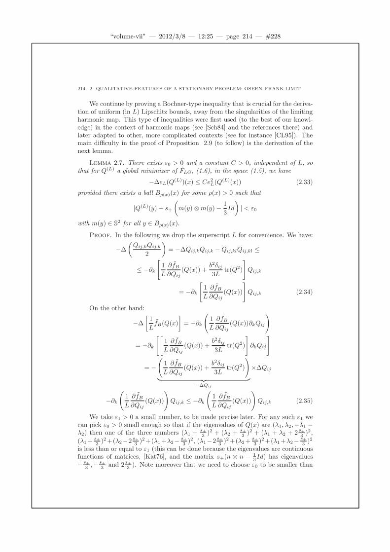
“volume-vii” — 2012/3/8 — 12:25 — page 214 — #228


We continue by proving a Bochner-type inequality that is crucial for the deriva-tion of uniform (in L) Lipschitz bounds, away from the singularities of the limitingharmonic map. This type of inequalities were first used (to the best of our knowl-edge) in the context of harmonic maps (see [Sch84] and the references there) andlater adapted to other, more complicated contexts (see for instance [CL95]). Themain difficulty in the proof of Proposition 2.9 (to follow) is the derivation of thenext lemma.

Lemma 2.7. There exists ε0 > 0 and a constant C > 0, independent of L, sothat for Q(L) a global minimizer of FLG, (1.6), in the space (1.5), we have

−∆eL(Q(L))(x) ≤ Ce2L(Q

(L)(x)) (2.33)

provided there exists a ball Bρ(x)(x) for some ρ(x) > 0 such that

|Q(L)(y)− s+

(m(y)⊗m(y)− 1

3Id

)| < ε0

with m(y) ∈ S2 for all y ∈ Bρ(x)(x).

Proof. In the following we drop the superscript L for convenience. We have:

−∆

(Qij,kQij,k

2

)= −∆Qij,kQij,k −Qij,klQij,kl ≤

≤ −∂k[1

L

∂fB∂Qij

(Q(x)) +b2δij3L

tr(Q2)

]Qij,k

= −∂k[1

L

∂fB∂Qij

(Q(x))

]Qij,k (2.34)

On the other hand:

−∆

[1

LfB(Q(x)

]= −∂k

(1

L

∂fB∂Qij

(Q(x))∂kQij

)

= −∂k[[

1

L

∂fB∂Qij

(Q(x)) +b2δij3L

tr(Q2)

]∂kQij

]

= −(1

L

∂fB∂Qij

(Q(x)) +b2δij3L

tr(Q2)

)

︸︷︷︸=∆Qij

×∆Qij

−∂k(

1

L

∂fB∂Qij

(Q(x))

)Qij,k ≤ −∂k

(1

L

∂fB∂Qij

(Q(x))

)Qij,k (2.35)

We take ε1 > 0 a small number, to be made precise later. For any such ε1 wecan pick ε0 > 0 small enough so that if the eigenvalues of Q(x) are (λ1, λ2,−λ1 −λ2) then one of the three numbers (λ1 + s+

3 )2 + (λ2 + s+3 )2 + (λ1 + λ2 + 2 s+

3 )2,

(λ1+s+3 )2+(λ2−2 s+

3 )2+(λ1+λ2− s+3 )2, (λ1−2 s+

3 )2+(λ2+s+3 )2+(λ1+λ2− s+

3 )2

is less than or equal to ε1 (this can be done because the eigenvalues are continuousfunctions of matrices, [Kat76], and the matrix s+(n ⊗ n − 1

3Id) has eigenvalues− s+

3 ,−s+3 and 2 s+

3 ). Note moreover that we need to choose ε0 to be smaller than

“volume-vii” — 2012/3/8 — 12:25 — page 215 — #229


the choice (of ε0) in Lemma 2.6 as we will need to use that lemma in the remainderof this proof.

For the matrix Q(x), let us denote its eigenvectors by n1(x), n2(x), n3(x) andlet λ1(x), λ2(x) , λ3(x) = −λ1(x) − λ2(x) denote the corresponding eigenvalues.From the preceeding discussion, we can, without loss of generality, assume that

(λ1 +s+3)2 + (λ2 +

s+3)2 + (λ1 + λ2 + 2

s+3)2 < ε1 (2.36)

We define the matrix

Qx def= −s+

3n1(x) ⊗ n1(x)−

s+3n2(x) ⊗ n2(x) +

2s+3n3(x)⊗ n3(x)

(Note that Qx = s+(n3(x) ⊗ n3(x)− 13Id)).

Taking into account (2.36) and the fact that Q(x) and Qx have the same eigen-vectors, we have :

tr(Q(x)−Qx)2 = (λ1 +s+3)2 + (λ2 +

s+3)2 + (λ1 + λ2 + 2

s+3)2 < ε1 (2.37)

Using the of Taylor expansion of 12

∂2fB∂Qij∂Qmn

(Q(x)) around Qx we obtain:

1

2

∂2fB∂Qij∂Qmn

(Q(x)) =1

2

∂2fB∂Qij∂Qmn

(Qx) +1

2

∂3fB∂Qij∂Qmn∂Qpq

(Qx)(Qpq(x) −Qxpq)

+Rijmn(Qx, Q(x))(2.38)

where Rijmn(Qx, Q(x)) is the remainder.From (2.38) we have:

−∂k(1

L

∂fB∂Qij

(Q(x)

)Qij,k = − 1

L

∂2fB∂Qij∂Qmn

Qmn,kQij,k =

= − 1

L

∂2fB∂Qij∂Qmn

(Qx)Qmn,kQij,k

︸︷︷︸≤0

− 1

L

∂3fB∂Qij∂Qmn∂Qpq

(Qx)(Qpq(x) −Qxpq)Qij,kQmn,k−

− 1

LRijmn(Q(x), Qx)Qij,kQmn,k ≤

≤ C0δ

L2Σ3

i,j,m,n=1

(∂3fB

∂Qij∂Qmn∂Qpq(Qx)

)2

(Qpq(x) −Qxpq)

2

+C0δ

L2

3∑

i,j,m,n=1

(Rijmn

)2(Q(x), Qx) +

1

δ|∇Q|4 ≤

“volume-vii” — 2012/3/8 — 12:25 — page 216 — #230


≤ δ

L2

3∑

i,j,m,n=1

[C0

(∂3f

∂Qij∂Qmn∂Qpq(Qx)

)2

+ C1

](Qpq(x) −Qx

pq)2 +

1

δ|∇Q|4

≤ C2δ

L2tr(Q(x)−Qx)2 +

1

δ|∇Q|4

(2.39)

where 0 < δ < 1 and C0, C0, C1, C2 are independent of L and x. For the first termin the second line above we use the fact that the Hessian matrix of a function fBis non-negative definite at a global minimum (which holds true in our case as well,

as one can easily check, even though we have fB restricted to the linear space S0).Let us recall (from the proof of the previous lemma) the definitions of F and

F . Then, for a matrix Q ∈ S0 with eigenvalues (λ1, λ2,−λ1 − λ2) we have

fB(Q) = F (λ1, λ2) (2.40)

We claim that for ε1 > 0 small enough there exists C2 independent of L, λ1, λ2so that

C2

((λ1 +

s+3)2 + (λ2 +

s+3)2 + (λ1 + λ2 + 2

s+3)2)≤ F (λ1, λ2)

for all (λ1, λ2) so that(λ1 +s+3)2 + (λ2 +

s+3)2 + (λ1 + λ2 + 2

s+3)2 < ε1. (2.41)

Careful computations show:

F (−s+3,−s+

3) =

∂F

∂λ1(−s+

3,−s+

3) =

∂F

∂λ2(−s+

3,−s+

3) = 0

∂2F

∂λ22(−s+

3,−s+

3) =

∂2F

∂λ21(−s+

3,−s+

3) =

1

4c2(b4 + 12a2c2 + b2

√b4 + 24a2c2)

∂2F

∂λ1∂λ2(−s+

3,−s+

3) = 3a2

Using a Taylor expansion around (λ1, λ2) = (− s+3 ,−

s+3 ) we have

F (λ1, λ2) =1

8c2

(b4 + 12a2c2 + b2

√b4 + 24a2c2

)[(λ1 +

s+3)2 + (λ2 +

s+3)2]+

+3a2(λ1 +s+3)(λ2 +

s+3) +R(λ1, λ2) ≥

≥ 1

2

1

8c2

(b4 + 12a2c2 + b2

√b4 + 24a2c2

)[(λ1 +

s+3)2 + (λ2 +

s+3)2]

+3a2

2(λ1 +

s+3)(λ2 +

s+3)

(2.42)

where R(λ1, λ2) is the remainder in the Taylor expansion, and the inequality holdsprovided that the remainder R is small enough. We choose ε1 > 0 to be smallenough so that if (λ1 +

s+3 )2 + (λ2 +

s+3 )2 + (λ1 + λ2 + 2 s+

3 )2 < ε1 then R is smallenough and the inequality above holds.

“volume-vii” — 2012/3/8 — 12:25 — page 217 — #231


As the quadratic form 116c2

(b4 + 12a2c2 + b2

√b4 + 24a2c2

)[(λ1 +

s+3 )2 +(λ2 +

s+3 )2]+ 3

2a2(λ1 +

s+3 )(λ2 +

s+3 ) is positive definite, there exists a C2 > 0, depending

only on a2,b2 and c2 such that

1

2

1

8c2

(b4 + 12a2c2 + b2

√b4 + 24a2c2

)[(λ1 +

s+3)2 + (λ2 +

s+3)2]

+3a2

2(λ1 +

s+3)(λ2 +

s+3)

≥ C2

((λ1 +

s+3)2 + (λ2 +

s+3)2 + (λ1 + λ2 +

2s+3

)2)

∀(λ1, λ2) ∈ R2

Combining this last inequality with (2.42) we obtain the claim (2.41).The relation (2.41) together with (2.40) and (2.37) show that tr(Q(x)−Qx)2 ≤

C3fB(Q(x)) for some C3 independent of L and x, which combined with (2.39) shows

−∂k(1

L

∂fB∂Qij

(Q(x)

)Qij,k ≤ δC4

L2fB(Q(x)) +

1

δ|∇Q(x)|4

with C4 a constant independent of L and x and any δ > 0. This last inequalitytogether with (2.34) and (2.35) show:

−∆eL +1

L2

3∑

i,j=1

(∂fB∂Qij

+b2δij3

tr(Q2)

)2

≤ δC4

L2fB(Q) +

1

δ|∇Q|4

Taking into account Lemma 2.6 and choosing δ small enough (depending only

on C4 and the constant C from Lemma 2.6) we can absorb the term δC4

L2 fB(Q) onthe right hand side into the left hand side and obtain

−∆eL ≤ 1

δ|∇Q|4,

giving the desired conclusion.

Lemma 2.8. Let Ω ⊂ R3 be a simply-connected bounded open set with smoothboundary. Let Q(Lk) ∈ W 1,2(Ω, S0) be a sequence of global minimizers for the

energy FLG, (1.6), in the admissible space (1.5). Assume that as Lk → 0 we haveQ(Lk) → Q(0) in W 1,2(Ω, S0).

Let K ⊂ Ω be a compact set which contains no singularity of Q(0). Thereexists C1 > 0, C2 > 0, L0 > 0( all constants independent of Lk) so that if fora ∈ K, 0 < r < d(a, ∂K) we have

1

r

∫

Br(a)

eLk(Q(Lk)(x)) dx ≤ C1

then

r2 supB r

2(a)

eLk(Q(Lk)) ≤ C2.

for all Lk < L0.

“volume-vii” — 2012/3/8 — 12:25 — page 218 — #232


Proof. Taking into account our assumptions on the sequence(Q(Lk)

)k∈N

,

Proposition 2.5 shows that for any given ε0 smaller than ε0 in Lemma 2.6 andalso smaller than the ε0 in Lemma 2.7, we have that there exists a L0 so that forLk < L0 we have

‖Q(Lk)(x)− s+

(n(x) ⊗ n(x)− 1

3Id

)‖ ≤ ε0, ∀x ∈ K, for some n(x) ∈ S

2 (2.43)

We continue reasoning similarly as in [Sch84]. We fix an arbitrary Lk < L0

and an a ∈ K and take a r > 0 so that 0 < r < d(a, ∂K). We let r1 > 0 andx1 ∈ Br1(a) be such that

max0≤s≤ 2

3 r(2

3r − s)2 max

Bs(a)eLk

(Q(Lk)) = (2

3r − r1)

2 maxBr1 (a)

eLk(Q(Lk))

= (2

3r − r1)

2eLk(Q(Lk)(x1)) (2.44)

Define e(Lk)1

def= maxBr1 (a)

eLk(Q(Lk)). Then:

maxB 2/3·r−r1

2

(x1)eLk

(Q(Lk)) ≤ maxB 2/3·r+r1

2

(a)eLk

(Q(Lk))

≤(2/3 · r − r1)

2 maxBr1(a)eLk

(Q(Lk))

(2/3 · r − (2/3 · r + r1)/2)2= 4 max

Br1(a)eLk

(Q(Lk)) = 4e(Lk)1 (2.45)

where for the first inequality we use the fact that B (2/3r−r1)2

(x1) ⊂ B (2/3·r+r1)2

(a)

and for the second inequality, we use the definition of r1.

Let r2 =(2/3·r−r1)

√

e(Lk)

1

2 and define R(Lk)(x) = Q(Lk)

(x1 +

x√

e(Lk)

1

). We let

Lk = e(Lk)1 Lk and then

eLk(R(Lk)) =

1

2|∇R(Lk)|2 + fB(R

(Lk))

Lk

=1

2

|∇Q(Lk)|2

e(Lk)1

+fB(Q

(Lk))

e(Lk)1 Lk

=1

e(Lk)1

eLk(Q(Lk))

Equation (2.45) then implies

maxx∈Br2(0)

eLk(R(Lk)) = max

x∈B (2/3r−r1)2

(x1)

eLk(Q(Lk)(x))

eLk1

≤ 4

where the equality above follows from the definitions of r2 and R(Lk) and theinequality above follows from equation (2.45). Thus, we have

maxBr2(0)

eLk(R(Lk)) ≤ 4, eLk

(R(Lk))(0) = 1 (2.46)

where R(Lk) satisfies the following system of elliptic PDEs

“volume-vii” — 2012/3/8 — 12:25 — page 219 — #233


LkR(Lk)ij,mm = −a2R(Lk)

ij −b2(R

(Lk)in R

(Lk)nj − δij

3tr((R(Lk))2)

)+c2R

(Lk)ij tr((R(Lk))2).

(2.47)We now claim that

r2 ≤ 1. (2.48)

It is clear that r2 ≤ 1 implies the conclusion. Let us assume for contradictionthat r2 > 1. Then we claim that there exists a constant C > 0 , independent ofLk, so that

1 ≤ C

∫

B1

eLk(R(Lk))(x) dx (2.49)

The matrix R(Lk) satisfies the system (2.47) (which is the rescaled version of(1.7) ); using relation (2.43) and the definition of R(Lk) as well as the fact thatr2 > 1, we can apply Lemma 2.7 to eLk

(R(Lk)) and obtain

−∆eLk(R(Lk)(x)) ≤ Ce2Lk

(R(Lk)(x))(2.46)

≤ 4CeLk(R(Lk)(x)), ∀x ∈ B1(0)

Combining (2.46) and the Harnack inequality (see for instance [Tay11], Ch.14,Thm. 9.3) along with the above relation we obtain (2.49).

We have∫

B1

eLk(R(Lk)(x)) dx ≤ 1

r2

∫

Br2 (0)

|∇R(Lk)(x)|22

+fB(R

(Lk)(x))

Lke(Lk)1

dx =

=2

2/3 · r − r1

∫

B(2/3·r−r1)/2(x1)

eLk(Q(Lk)(x)) dx ≤ 3

r

∫

Br/3(x1)

eLk(Q(Lk)(x)) dx

≤ 3

r

∫

Br(a)

eLk(Q(Lk)(x)) dx ≤ 3C1 (2.50)

where for the first inequality we use the monotonicity inequality (Lemma 2.2) andthe assumption that r2 ≥ 1 (note that the equation satisfied by R(Lk) , equa-tion (2.47) is the same as the equation satisfied by Q(Lk), up to a different elasticconstant, hence the use of Lemma 2.2 here is justified). For the equality in re-lation (2.50) we use the change of variables y = x1 +

x√

eLk1

and use the relation:

eLk(R(Lk)) = 1

e(Lk)

1

eLk(Q(Lk)). For the second inequality in (2.50) we use the mono-

tonicity inequality and the fact that 2/3r−r12 ≤ r

3 . For the third inequality in (2.50)

we use the fact that Br/3(x1) ⊂ Br(a) since |x1 − a| < r1 <23r. The last step in

(2.50) follows from the hypothesis of the Lemma.Choosing C1 small enough we reach a contradiction with (2.49) which in turn

implies that r2 ≤ 1 and hence the conclusion.

We can now prove the uniform convergence of Q(Lk) away from singularities ofthe limiting harmonic map Q(0):

Proposition 2.9. Let Ω ⊂ R3 be a simply-connected bounded open set withsmooth boundary. Let Q(Lk) ∈ W 1,2(Ω, S0) be a sequence of global minimizers for

“volume-vii” — 2012/3/8 — 12:25 — page 220 — #234


the energy FLG, (1.6), in the admissible space (1.5). Assume that as Lk → 0 wehave Q(Lk) → Q(0) in W 1,2(Ω, S0).

Let K ⊂ Ω be a compact set which contains no singularity of Q(0). Then

limk→∞

Q(Lk)(x) = Q(0)(x), uniformly for x ∈ K. (2.51)

Proof. From the hypothesis and Proposition 2.5 we have that fB(Q(Lk)) → 0

uniformly in K. Thus for any ε0 > 0 there exists a L0 > 0 such that for Lk < L0

we have that |Q(Lk)(x)− s+(n(x)⊗ n(x) − 1

3Id)| < ε0 for all x ∈ K (and for each

x ∈ K, we have n(x) ∈ S2). Thus we can apply Lemmas 2.6, 2.7 and 2.8.Recall that we have Q(Lk) → Q(0) in W 1,2. In order to show the uniform

convergence it suffices to show that we have uniform (independent of Lk) Lipschitzbounds on Q(Lk) for x ∈ K. We reason similarly to the proof in Proposition 2.5(see also [CL95]). We first claim that there exists an ε1 > 0 so that

∀ε ∈ (0, ε1), there exists r0(ε) depending only on ε, Ω,K,

and boundary data Qb so that

1

r0

∫

K∩Br0 (x)

1

2|∇Q(Lk)(x)|2 + fB(Q

(Lk)(x))

Lkdx ≤ ε , ∀x ∈ K,

provided that Lk < L∗(ε, r0(ε)) (2.52)

In order to prove the claim let us first recall that Q(0) has no singularities onthe compact set K. Thus there exists a larger compact set K ′ with K ⊂ K ′ anda constant C > 0 so that |∇Q(0)(x)| ≤ C, ∀x ∈ K ′. We choose ε1 > 0 so thatB(x, ε1) ∩K ⊂ K ′ hence for an arbitrary ε ∈ (0, ε1) there exists r0(ε) > 0 so that

1

r0

∫

K∩Br0(x)

1

2|∇Q(0)(x)|2 dx < ε

3

provided that x ∈ K and r0(ε) is chosen small enough. We also have, from theW 1,2(Ω, S0) convergence of Q

(Lk) to Q(0), that there exists L(ε) so that

1

r0

∫

K∩Br0(x)

1

2|∇Q(Lk)(x)|2 dx ≤ 1

r0

∫

K∩Br0(x)

1

2|∇Q(0)(x)|2 dx+

ε

3, ∀Lk < L(ε)

Recall from the proof of Lemma 2.3 that limLk→0

∫Ω

fB(Q(Lk)(x))Lk

dx = 0. Hence

there exists L(ε) so that 1r0

∫K∩Br0(x)

fB(Q(Lk)(x))Lk

dx < ε3 , ∀L < L(ε). Letting

L∗(ε, r0(ε)) = minL, L and combining the two relations above we obtain theclaim (2.52).

Choosing ε > 0 smaller than the constant C1 from Lemma 2.8, we applyLemma 2.8 to conclude that |∇Q(Lk)| can be bounded, independently of Lk, onthe set K. The uniform convergence result now follows.

3. Biaxiality and uniaxiality

3.1. The bulk energy density. Our first proposition concerns the stationarypoints of the bulk energy density.

“volume-vii” — 2012/3/8 — 12:25 — page 221 — #235

3. BIAXIALITY AND UNIAXIALITY 221

Proposition 3.1. [BM10] Consider the bulk energy density fB(Q) given by

fB(Q) = −a2

2trQ2 − b2

3trQ3 +

c2

4

(trQ2

)2+a2

3s2+ +

2b2

27s3+ − c2

9s4+. (3.1)

Then fB(Q) attains its minimum for uniaxial Q-tensors of the form

Q = s+

(n⊗ n− 1

3

), (3.2)

where

s+ =b2 +

√b4 + 24a2c2

4c2(3.3)

and n : Ω → S2 is a unit eigenvector of Q.

Proof. Proposition 3.1 was proved in [BM10] and we reproduce the proof inthe Appendix for completeness.

In the following proposition, we estimate fB(Q) in terms of |Q| and the biaxi-ality parameter β(Q).

Proposition 3.2. Let Q ∈ S0. Then the bulk energy density fB(Q) is boundedfrom below by

fB(Q) ≥ Γ(a2, b2, c2)

(|Q| −

√2

3s+

)2

+b2

6√6β(Q)|Q|3 (3.4)

where

Γ(a2, b2, c2) =b2

216c2

3√b4 + 24a2c2 − b2

(3.5)

and s+ has been defined in (3.3).

Proof. From Lemma 0.5, we have the inequality,

trQ3 = |Q|3√(

1− β

6

)≤ |Q|3√

6

(1− β

2

)for Q ∈ S0.

From the definition of fB(Q) and s+ in (3.1) and (3.3), we can obtain a lower

bound for fB(Q) in terms of |Q| and β(Q) as follows i.e.

fB(Q) = −a2

2|Q|2 − b2

3√6|Q|3

√1− β +

c2

4|Q|4 + a2

2

(√2

3s+

)2

+b2

3

2s3+9

− c2

4

(√2

3s+

)4

(3.6)

≥[−a

2

2|Q|2 − b2

3√6|Q|3 + c2

4|Q|4 + a2

3s2+ +

2b2

27s3+ − c2

9s4+

]+

b2

6√6β(Q)|Q|3.

(3.7)

“volume-vii” — 2012/3/8 — 12:25 — page 222 — #236


The bracketed term in (3.7) can be further simplified by carrying out a series of

calculations. Let δ = |Q| −√

23s+ where 2

3c2s2+ = b2√

6

√23s+ + a2 by the definition

of s+. Then[−a

2

2|Q|2 − b2

3√6|Q|3 + c2

4|Q|4 + a2

3s2+ +

2b2

27s3+ − c2

9s4+

]= (3.8)

= δ

[−a2

√2

3s+ −

√2b2

3√3s2+ +

2√2

3√3c2s3+

]+ δ2

[−a

2

2− b2

3s+ + s2+c

2

]+

+δ3

[c2√

2

3s+ − b2

3√6

]+c2

4δ4. (3.9)

The coefficient of δ vanishes from the definition of s+. Therefore, we have that[−a

2

2|Q|2 − b2

3√6|Q|3 + c2

4|Q|4 + a2

3s2+ +

2b2

27s3+ − c2

9s4+

]= (3.10)

= δ2(α+ βδ + γδ2

)where

α =

[−a

2

2− b2

3s+ + s2+c

2

]=a2

2+c2s2+3

β =

[c2√

2

3s+ − b2

3√6

]≥ 2b2

3√6> 0 and

γ =c2

4. (3.11)

It is readily verified that the function

f(δ) =(α+ βδ + γδ2

)

attains its minimum value at δmin = − β2γ and the minimum value is

f(δmin) =b2

216c2

3√b4 + 24a2c2 − b2

. (3.12)

Substituting (3.12) into (3.10), we have that[−a

2

2|Q|2 − b2

3√6|Q|3 + c2

4|Q|4 + a2

3s2+ +

2b2

27s3+ − c2

9s4+

]≥ Γ(a2, b2, c2)δ2 (3.13)

where Γ has been defined in (3.5) and on combining (3.13) with (3.7), the lowerbound (3.4) follows.

We can obtain explicit lower bounds for fB in terms of the order parameters sand r in Proposition 0.1, as shown below.

Proposition 3.3. Let Q ∈ S0 be represented as in Proposition 0.1

Q = s

(n⊗ n− 1

3Id

)+ r

(m⊗m− 1

3Id

)

with either 0 ≤ r ≤ s2 or s

2 ≤ r ≤ 0. Case (i) Non-negative order parameters,0 ≤ r ≤ s

2 with 0 ≤ s ≤ s+, where s+ is defined in (3.3). Then the bulk energy

“volume-vii” — 2012/3/8 — 12:25 — page 223 — #237


density, fB(Q), is bounded from below by

fB(Q) ≥ (s+ − s)2 γ(a2, b2, c2) +r(s − r)

9

(3a2 + b2s− 2c2s2

)+

5b2

27r2s ≥ 0

0 ≤ s ≤ s+ (3.14)

where γ(a2, b2, c2

)is an explicitly computable positive constant.

Case (ii) Non-negative order parameters, 0 ≤ r ≤ s2 and s ≥ s+. Then

fB(Q) ≥ b2

216c2

3(b4 + 24a2c2)1/2 − b2

min

2

3(s− s+)

2,1

6

(√3s− 2s+

)2

+τb2s3+

(r2(s− r)2

s4

)

(3.15)

where τ is an explicitly computable positive constant, independent of a2, b2, c2.Case (iii) If s

2 ≤ r ≤ 0, then

fB(Q) = fB(−Q) +2b2

27

(2|s|3 + 2|r|3 − 3s2|r| − 3|s|r2

), (3.16)

where −Q ∈ S0 has positive order parameters 0 ≤ −r ≤ − s2 and fB(−Q) can be

estimated using (3.14) and (3.15). In particular,

fB(Q) ≥ − a4

4c2− s3+

3

(b2

9− c2

3s+

)> 0 (3.17)

for Q-tensors with s2 ≤ r ≤ 0.

Proof. From Proposition 0.1, it suffices to consider the two cases 0 ≤ r ≤ s2

and s2 ≤ r ≤ 0.

Case (i): We can explicitly express the bulk energy density, fB(Q), in terms ofs and r as follows –

fB(Q) = −a2

3

(s2 + r2 − sr

)− b2

27

(2s3 + 2r3 − 3s2r − 3sr2

)

+c2

9

(s4 + r4 + 3s2r2 − 2sr3 − 2s3r

)+a2

3s2+ +

2b2

27s3+ − c2

9s4+, (3.18)

where we have expressed trQ2 and trQ3 in terms of s and r

trQ2 =2

3

(s2 + r2 − sr

)

and

trQ3 =1

9

(2s3 + 2r3 − 3s2r − 3sr2

).

The function fB(Q) consists of two components – fB(Q) = F (s) +G(s, r), where

F (s) = −a2

3

(s2 − s2+

)− 2b2

27

(s3 − s3+

)+c2

9

(s4 − s4+

)

G(s, r) =a2

3

(sr − r2

)+b2

27

(3s2r + 3sr2 − 2r3

)+c2

9

(−2s3r + 3s2r2 − 2sr3 + r4

).

(3.19)

“volume-vii” — 2012/3/8 — 12:25 — page 224 — #238


Recalling that 2c2s2+ = b2s+ + 3a2 (from the definition of s+ in (3.3)), thefunction F (s) can be expressed in terms of δ = s+ − s ≥ 0 as follows –

F (s) =δ

27

(18a2s+ + 6b2s2+ − 12c2s3+

)

+ δ2(3b2

27s+ +

18a2

27+ δ

(2b2

27− 4c2

9s+ +

c2

9δ

)). (3.20)

The coefficient of δ vanishes by virtue of the definition of s+ in (3.3). We note thatthe function

G (δ)def= δ

(2b2

27− 4c2

9s+ +

c2

9δ

)(3.21)

attains a minimum for

δmin = 2s+ − b2

3c2> s+ (3.22)

and, since G is non-increasing on [δ, s+]:

G(δ) ≥ G(s+) =1

27

(2b2s+ − 9c2s2+

). (3.23)

We substitute (3.23) into (3.20) to obtain the following lower bound for F (s) -

F (s) ≥ c2s2+ + 3a2

27(s+ − s)

2. (3.24)

We can analyze the function G(s, r), in (3.19), in an analogous manner. Letγ = r

s ∈[0, 12]. Then

G(s, r) = γs2[a2

3+

3b2

27s− 2c2

9s2]+ γ2s2

[−a

2

3+

3b2

27s+

3c2

9s2]

+γ3s3[−2b2

27− 2c2s

9+ γ

c2s

9

]. (3.25)

The coefficient of γ is non-negative for all s ≤ s+. Using the inequality γ ≤ 12 , one

readily obtains the following lower bound for G(s, r) -

G(s, r) ≥ γs2[a2

3+

3b2

27s− 2c2

9s2]+ γ2s2

[−a

2

3+

2b2

27s+

2c2

9s2]≥

≥ r(s − r)

9

(3a2 + b2s− 2c2s2

)+

5b2

27r2s. (3.26)

Combining (3.24) and (3.26), the lower bound for 0 ≤ s ≤ s+ in (3.14) follows.Case (ii) The case s ≥ s+ can be dealt with similarly. For any Q ∈ S0 with

0 ≤ r ≤ s2 , we have that

s√2≤ |Q| =

√2

3

√(s2 + r2 − sr) ≤

√2

3s. (3.27)

For s ≥ s+, |Q|3 ≥ s3+2√2and

β(Q) ≥ η

(r2(s− r)2

s4

)(3.28)

“volume-vii” — 2012/3/8 — 12:25 — page 225 — #239


where β(Q) is the biaxiality parameter defined in (0.9) and η is a positive constantindependent of a2, b2 or c2 or L. Combining (3.27), (3.28) and (3.4), we readilyobtain the lower bound

fB(Q) ≥ b2

216c2

3(b4 + 24a2c2)1/2 − b2

(|Q| −

√2

3s+

)2

+b2

6√6β(Q)|Q|3 ≥

≥ b2

216c2

3(b4 + 24a2c2)1/2 − b2

min

2

3(s− s+)

2 ,1

6

(√3s− 2s+

)2

+τb2s3+

(r2(s− r)2

s4

)

(3.29)

where τ is an explicitly computable positive constant.Case (iii) Finally, we consider Q ∈ S0 with negative order parameters s

2 ≤ r ≤0. In this case, one can directly check that

trQ3 =1

9

(2s3 + 2r3 − 3s2r − 3sr2

)≤ 0

and therefore,

fB(Q) = −a2

2|Q|2 − b2

3trQ3 +

c2

4|Q|4 + a2

3s2+ +

2b2

27s3+ − c2

9s4+

= −a2

2|Q|2 − b2

3tr (−Q)3 +

c2

4|Q|4 + a2

3s2+ +

2b2

27s3+ − c2

9s4+ +

2b2

3

∣∣trQ3∣∣ ,

(3.30)

since b2

3 tr (−Q)3 = − b2

3 trQ3 and − b2

3 trQ3 = b2

3

∣∣trQ3∣∣. The equality (3.16)

follows from (3.30) upon expressing trQ3 in terms of s and r.For (3.17), it suffices to note that for s, r ≤ 0, trQ3 ≤ 0 and therefore,

fB(Q) ≥ −a2

2|Q|2 + c2

4|Q|4 + a2

3s2+ +

2b2

27s3+ − c2

9s4+

= −a2

3

(s2 + r2 − sr

)+c2

9

(s2 + r2 − sr

)2 − s3+3

(b2

9− c2

3s+

). (3.31)

A straightforward computation shows that the function

−a2

3

(s2 + r2 − sr

)+c2

9

(s2 + r2 − sr

)2 ≥ − a4

4c2

ands3+3

(b2

9− c2

3s+

)< − a4

4c2.

The inequality (3.17) now follows.

Remark 3.4. One can readily obtain lower bounds for fB(Q) in terms of the or-der parameters (S, R) in Proposition 0.3, following the methods outlined in Propo-sition 3.3. The details are omitted here for brevity.

“volume-vii” — 2012/3/8 — 12:25 — page 226 — #240


Remark 3.5. Relation (3.17) shows that if fB(Q(Lk)(x)) → 0 as Lk → 0 then

Q(Lk)(x) cannot have an (s, r) representation with s2 < r < 0, if Lk is sufficiently

small.

In view of Propositions 2.1 and 3.2, we can make qualitative predictions aboutthe size of regions where a global Landau–De Gennes minimizer Q∗ can have

|Q∗| <<√

23s+ and the size of regions where Q∗ can be strongly biaxial.

Proposition 3.6. Let Q∗ be a global minimizer of FLG, (1.6), in the space

(1.5). Let Ω∗ =x ∈ Ω; |Q∗(x)| ≤ 1

2

√23s+

. Then

|Ω∗| ≤ αL

Γ(a2, b2, c2)

∫

Ω

|∇n(0)(x)|2 dx, (3.32)

where n(0) is defined in (1.9) and α is an explicitly computable positive constantindependent of a2, b2, c2 or L. The constant Γ(a2, b2, c2) is defined in (3.5).

Proof. From Proposition 3.2, we have that

fB(Q∗(x)) ≥ 1

αΓs2+, x ∈ Ω∗ (3.33)

for some explicitly computable positive constant α, since |Q∗| ≤ 12

√23s+ = 1√

6s+

on Ω∗. On the other hand, recalling the definition of Q(0) in (1.8) and since Q∗ is

a global minimizer of FLG[Q], we have that∫

Ω∗

fB(Q∗(x)) dx ≤ FLG[Q

(0)] =

∫

Ω

L

2|∇Q(0)|2+fB(Q(0)) dx = Ls2+

∫

Ω

|∇n(0)|2 dx,(3.34)

since fB(Q(0)) = 0 everywhere in Ω. Substituting (3.33) into (3.34), we obtain

1

αΓ(a2, b2, c2)s2+|Ω∗| ≤ Ls2+

∫

Ω

|∇n(0)|2 dx, (3.35)

from which the inequality (3.32) follows.

Proposition 3.7. Let Q∗ be a global minimizer of FLG, (1.6), in the space(1.5). Let

Ωλ =

x ∈ Ω; |Q∗(x)| ≥ 1

2

√2

3s+, β(Q(x)) > λ

for some positive constant λ. Then,

|Ωλ| ≤ αL

λs+b2

∫

Ω

|∇n(0)|2 dx (3.36)

where n(0) is defined in (1.9) and α is an explicitly computable positive constantindependent of a2, b2, c2 or L.

Proof. From Proposition 3.2, we have that

fB(Q∗(x)) ≥ b2

6√6β(Q∗(x))|Q∗(x)|3 ≥ 1

αb2λs3+ x ∈ Ωλ (3.37)

“volume-vii” — 2012/3/8 — 12:25 — page 227 — #241


for some explicitly computable positive constant α, since |Q∗| ≥ 12

√23s+ = 1√

6s+

on Ωλ. On the other hand, recalling the definition of Q(0), (1.8), and since Q∗ is a

global minimizer of FLG[Q], we have that∫

Ωλ

fB(Q∗(x)) dx ≤

∫

Ω

L

2|∇Q(0)|2 + fB(Q

(0)) dx = Ls2+

∫

Ω

|∇n(0)|2 dx (3.38)

since fB(Q(0)) = 0 everywhere in Ω. Substituting (3.37) into (3.38), we obtain

1

αb2λs3+|Ωλ| ≤ Ls2+

∫

Ω

|∇n(0)|2 dx, (3.39)

from which the inequality (3.36) follows.

Proposition 3.6 is relevant to the size of defect cores in global energy minimizerswhereas Proposition 3.7 is relevant to the equilibrium behaviour far away from thedefect cores.

3.2. Analyticity and uniaxiality. We define a new biaxiality parameterβ(Q) as follows:

β(Q)def= (tr(Q2))3 − 6(tr(Q3))2.

Then β(Q) ≥ 0 with β(Q) = 0 if and only if Q is uniaxial i.e. Q = s(n⊗ n− 1

3Id)

for some s ∈ R\0, n ∈ S2 or Q = 0. The function β(Q) is a real analytic function

of Q and this is particularly important given that global energy minimizers of FLG

in the admissible space AQ are real analytic:

Proposition 3.8. Let Ω be a simply-connected bounded open set with smoothboundary. Let Q(L) be a global minimizer of FLG, (1.6), in the space (1.5). Thisglobal minimizer Q(L) is a solution of (1.7) and is real analytic in Ω.

Proof. We drop the superscript L fromQ(L) for convenience. As−a2

2 tr(Q2)−

b2

3 tr(Q3)+ c2

4

(trQ2

)2is bounded from below (see also the Appendix) we have that

there exists an H1-global energy minimizer. This is a weak solution of the Euler-Lagrange system:

L∆Qij = −a2Qij − b2(QikQkj −

δij3

tr(Q2)

)+ c2Qij tr(Q

2)

For Q an H1 solution of the equation one uses H1 → L6 (in R3) and Holder’s

inequality to obtain that the right hand side of each equation is in L2. Elliptic regu-larity gives that Q ∈ H2 →W 1,6 → L∞ hence the right hand side of each equationis in H1. Elliptic regularity gives Q ∈ H3 and one can continue bootstrapping toobtain the C∞ regularity.

We obtain the analyticity by observing that the nonlinearity is polynomial andthen standard results (see for instance [Fri58], p.45) imply that that the solutionsare real analytic in Ω.

Proposition 3.9. Let Q be a real analytic function Q : Ω ⊂ R3 → S0. Thenthe set where Q is uniaxial or isotropic is either Ω itself or has zero Lebesguemeasure.

“volume-vii” — 2012/3/8 — 12:25 — page 228 — #242


Proof. If there is no x ∈ Ω such that β(Q(x)) 6= 0 then Q is uniaxial or

isotropic everywhere. If there exists a P ∈ Ω such that β(Q(P )) 6= 0 then let usconsider the lines passing through P . The restriction of Q to any such line is realanalytic and then so is β(Q). Thus β(Q) has at most countably many zeroes on

such a line. We claim that this implies that the set of zeroes of β(Q) in Ω is ofmeasure zero.

We assume, without loss of generality, that P = 0. We denote N∗ = N \ 0and decompose Ω = ∪n∈N∗

(B 1

n\B 1

n+1∩ Ω

)∪(∪n∈N∗

(Bn+1 \Bn ∩ Ω

))∪ 0.

We claim that for any n ∈ N∗ the set(β(Q)

)−1

(0) ∩(Ω ∩B 1

n\B 1

n+1

)is a set of

measure zero. This implies that β(Q)−1(0) ∩ Ω, which is a countable union of setsas before, is also a set of measure zero.

We consider the bi-Lipschitz functions

fn : [1

n+ 1,1

n]× [0, π]× [0, 2π) → B 1

n\B 1

n+1, ∀n ∈ N

that realize the change of coordinates from polar to usual cartesian coordinates.

We have that f−1n

(β(Q)−1(0) ∩ Ω ∩B 1

n\B 1

n+1

)⊂ [ 1

n+1 ,1n ] × [0, π] × [0, 2π).

We recall that the Lebesgue measure µ on the 3-dimensional product space [ 1n+1 ,

1n ]×

[0, π] × [0, 2π) is the completion of the product measure µ1 × µ2 where µ1 is the1-dimensional Lebesgue measure on [ 1

n+1 ,1n ] and µ2 is the 2-dimensional Lebesgue

measure on [0, π]× [0, 2π). Then for any set E ⊂ [ 1n+1 ,

1n ]× [0, π]× [0, 2π) we have

(µ1 × µ2)(E) =

∫

[0,π]×[0,2π)

µ1(Ey)µ2(dy)

where Ey = x ∈ [ 1n+1 ,

1n ], (x, y1, y2) ∈ E ⊂ [ 1

n+1 ,1n ]. In our case, letting

Edef= f−1

n

(β(Q)−1(0) ∩ Ω ∩B 1

n\B 1

n+1

)

we have that Ey is made of finitely many points for almost all y ∈ [0, π]×[0, 2π)(thisis a consequence of the first paragraph in this proof. Indeed, on the segment

through P that is in Ω∩B 1n\B 1

n+1and has direction given in polar coordinates by

y ∈ [0, π]× [0, 2π) there are only finitely many points that are isotropic or uniaxial.The set Ey is just the set of the distances to P of the uniaxial or isotropic pointsthat are on such a segment). Thus µ1(E

y) = 0, µ2 − a.e. y hence µ1 × µ2(E) = 0thus µ(E) = 0.

As bi-Lipschitz functions carry sets of measure zero into sets of measure zero

we have that β(Q)−1(0) ∩ Ω ∩ B 1n\B 1

n+1is a set of measure zero for all n ∈ N.

A similar argument holds for the sets β−1(0) ∩ Ω ∩ Bn+1 \Bn for all n ∈ N. On

the other hand β(Q)−1(0) ∩ Ω is a countable union of sets as before, hence it hasmeasure zero.

Corollary 3.10. Let Q(L) be a global minimizer of FLG, (1.6), in the space(1.5). Then there exists a set of Lebesgue measure zero, possibly empty, Ω0 inΩ such that the eigenvectors of Q(L) are smooth at all points x ∈ Ω \ Ω0. The

“volume-vii” — 2012/3/8 — 12:25 — page 229 — #243


uniaxial-biaxial, isotropic-uniaxial or isotropic-biaxial interfaces are contained inΩ0.

Proof. The global minimizer Q(L) ∈ C∞ (Ω;S0). The eigenvectors of Q(L)

have the same degree of regularity as Q(L) on sets K ⊂ Ω, where Q(L) has aconstant number of distinct eigenvalues i.e. where Q(L) is either biaxial or uniaxialor isotropic, [Nom73], but not necessarily otherwise [Kat76]. If Q(L) is uniaxialeverywhere then Ω0 = ∅. If Q(L) is either uniaxial or isotropic on the whole ofΩ (i.e. β(Q(L)) = 0 in Ω), with Q(L) 6= 0 at some point in Ω, then let Ω =

x ∈ Ω, Q(L)ij = 0, i, j = 1, 2, 3 denote the zero-set of Q(L). Let us observe that

Ω =(|Q|2

)−1(0) and |Q|2 is an analytic function. By an argument similar to the

proof of Proposition 3.9 and since Q(x) 6= 0 for at least one point x ∈ Ω, we have

that Ω has measure zero and we take Ω0def= Ω.

If Q(L) is biaxial somewhere then Proposition 3.9 shows that the set of pointswhere β(Q) = 0 has measure zero. We denote this set by Ω0 and observe that Ω\Ω0

is an open set and the eigenvectors have the same regularity as Q(L) on Ω \Ω0, see[Nom73].

“volume-vii” — 2012/3/8 — 12:25 — page 230 — #244

“volume-vii” — 2012/3/8 — 12:25 — page 231 — #245

CHAPTER 3

Well-posedness of a dynamical model: Q-tensors

and Navier–Stokes

In this chapter we consider the Beris and Edwards model as described in Sec-tion 4 but restrict ourselves to the case ξ = 0. This means that the molecules aresuch that they only tumble in a shear flow, but are not aligned by such a flow. Inthis case the system (4.3) reduces to:

(∂t + uγ · ∂γ)Qαβ − ΩαγQγβ +QαγΩγβ

= Γ(L∆Qαβ − aQαβ + b[QαγQγβ − δαβ

d tr(Q2)]− cQαβ tr(Q2))

∂tuα + uβ∂βuα = ν∆uα + ∂αp− L∂β

(∂αQζδ∂βQζδ − δαβ

d ∂λQζδ∂λQζδ

)

+L∂β (Qαγ∆Qγβ −∆QαγQγβ)∂γuγ = 0

(0.1)in R

d, d = 2, 3.We also need to assume from now on that

c > 0 (0.2)

This assumption is necessary from a modelling point of view (see [Maj10],[MZ10] )so that the energy F (see next section, relation (1.1)) is bounded from below, andit is also necessary for having global solutions (see Proposition 1.2 and its proof).The presentation follows ideas from [PZ].

1. The dissipation and apriori estimates

Let us denote the free energy of the director fields:

F(Q) =

∫

Rd

L

2|∇Q|2 + a

2tr(Q2)− b

3tr(Q3) +

c

4tr2(Q2) dx (1.1)

In the absence of the flow, when u = 0 in the equations (0.1), the free energy isa Lyapunov functional of the system. If u 6= 0 we still have a Lyapunov functionalfor (0.1) but this time one that includes the kinetic energy of the system. Moreprecisely we have:

Proposition 1.1. The system (0.1) has a Lyapunov functional:

E(t)def=

1

2

∫

Rd

|u|2(t, x) dx +

∫

Rd

L

2|∇Q|2(t, x)

+a

2tr(Q2(t, x)) − b

3tr(Q3(t, x)) +

c

4tr2(Q2(t, x)) dx (1.2)

231

“volume-vii” — 2012/3/8 — 12:25 — page 232 — #246

232 3. WELL-POSEDNESS OF A DYNAMICAL MODEL: Q-TENSORS AND NAVIER–STOKES

If d = 2, 3 and (Q, u) is a smooth solution of (0.1) such that Q ∈L∞(0, T ;H1(Rd))∩L2(0, T ;H2(Rd)) and u ∈ L∞(0, T ;L2(Rd))∩L2(0, T ;H1(Rd))then, for all t < T , we have:

d

dtE(t) = −ν

∫

Rd

|∇u|2 dx

− Γ

∫

Rd

tr

(L∆Q− aQ+ b[Q2 − tr(Q2)

3Id]− cQ tr(Q2)

)2

dx ≤ 0 (1.3)

Proof. We multiply the first equation in (0.1) to the right by

−(L∆Q− aQ+ b[Q2 − tr(Q2)

3Id]− cQ tr(Q2)

),

take the trace, integrate over Rd and by parts and sum with the second equationmultiplied by u and integrated over Rd and by parts (let us observe that becauseof our assumptions on Q and u we do not have boundary terms, when integratingby parts). We obtain:

d

dt

∫

Rd

1

2|u|2 + L

2|∇Q|2 + a

2tr(Q2)− b

3tr(Q3) +

c

4tr2(Q2) dx

+ν

∫

Rd

|∇u|2 dx+ Γ

∫

Rd

tr

(L∆Q− aQ+ b[Q2 − tr(Q2)

3Id]− cQ tr(Q2)

)2

dx

=

∫

Rd

u · ∇Qαβ

(−aQαβ + b[QαγQγβ − δαβ

3tr(Q2)]− cQαβ tr(Q

2))

)dx

︸︷︷︸I

+

∫

Rd

(−ΩαγQγβ +QαγΩγβ)

(−aQαβ + b[QαδQδβ − δαβ

3tr(Q2)]− cQαβ tr(Q

2))

)dx

︸︷︷︸II

+L

∫

Rd

uγQαβ,γ∆Qαβ dx

︸︷︷︸A

−L2

∫

Rd

uα,γQγβ∆Qαβ dx

︸︷︷︸B

+L

2

∫

Rd

uγ,αQγβ∆Qαβ

︸︷︷︸C

dx+L

2

∫

Rd

Qαγuγ,β∆Qαβ dx

︸︷︷︸C

−L2

∫

Rd

Qαγuβ,γ∆Qαβ dx

︸︷︷︸B

+L

∫

Rd

Qγδ,αQγδ,βuα,β dx

︸︷︷︸AA

−L∫

Rd

Qαγ∆Qγβuα,β dx+ L

∫

Rd

∆QαγQγβuα,β dx

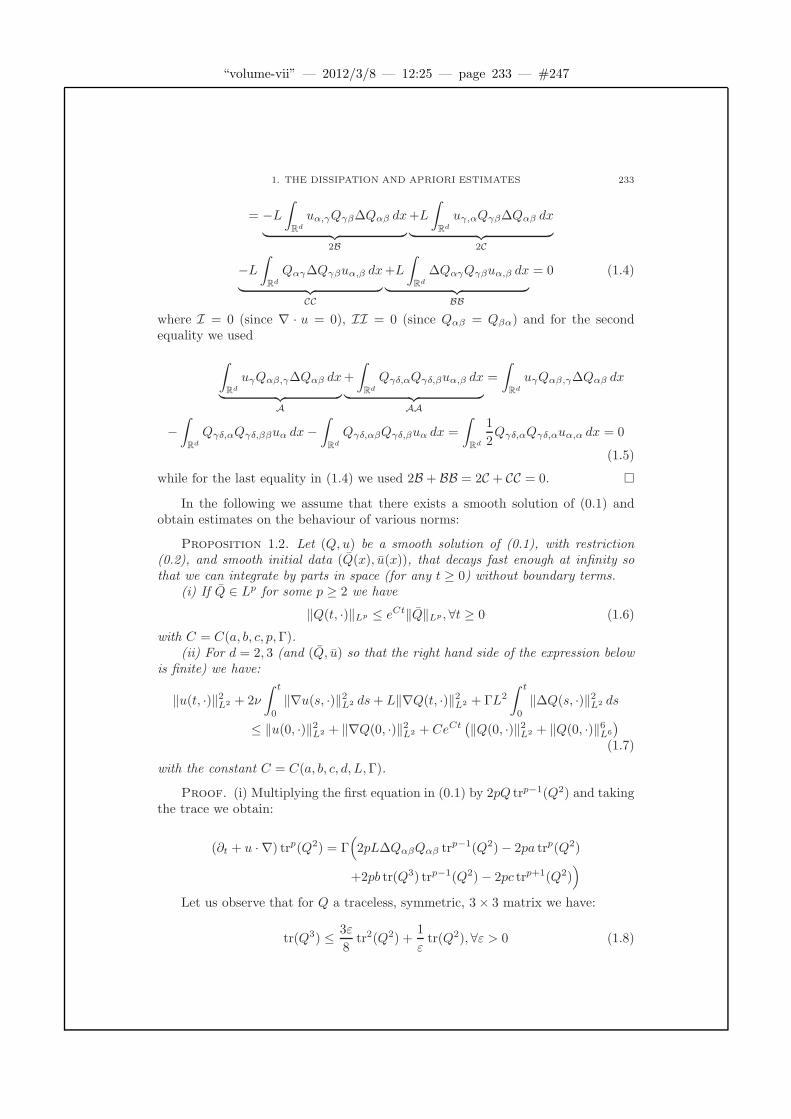
“volume-vii” — 2012/3/8 — 12:25 — page 233 — #247

1. THE DISSIPATION AND APRIORI ESTIMATES 233

= −L∫

Rd

uα,γQγβ∆Qαβ dx

︸︷︷︸2B

+L

∫

Rd

uγ,αQγβ∆Qαβ dx

︸︷︷︸2C

−L∫

Rd

Qαγ∆Qγβuα,β dx

︸︷︷︸CC

+L

∫

Rd

∆QαγQγβuα,β dx

︸︷︷︸BB

= 0 (1.4)

where I = 0 (since ∇ · u = 0), II = 0 (since Qαβ = Qβα) and for the secondequality we used

∫

Rd


︸︷︷︸A

+

∫

Rd

Qγδ,αQγδ,βuα,β dx

︸︷︷︸AA

=

∫

Rd


−∫

Rd

Qγδ,αQγδ,ββuα dx−∫

Rd

Qγδ,αβQγδ,βuα dx =

∫

Rd

1

2Qγδ,αQγδ,αuα,α dx = 0

(1.5)

while for the last equality in (1.4) we used 2B + BB = 2C + CC = 0.

In the following we assume that there exists a smooth solution of (0.1) andobtain estimates on the behaviour of various norms:

Proposition 1.2. Let (Q, u) be a smooth solution of (0.1), with restriction(0.2), and smooth initial data (Q(x), u(x)), that decays fast enough at infinity sothat we can integrate by parts in space (for any t ≥ 0) without boundary terms.

(i) If Q ∈ Lp for some p ≥ 2 we have

‖Q(t, ·)‖Lp ≤ eCt‖Q‖Lp , ∀t ≥ 0 (1.6)

with C = C(a, b, c, p,Γ).(ii) For d = 2, 3 (and (Q, u) so that the right hand side of the expression below

is finite) we have:

‖u(t, ·)‖2L2 + 2ν

∫ t

0

‖∇u(s, ·)‖2L2 ds+ L‖∇Q(t, ·)‖2L2 + ΓL2

∫ t

0

‖∆Q(s, ·)‖2L2 ds

≤ ‖u(0, ·)‖2L2 + ‖∇Q(0, ·)‖2L2 + CeCt(‖Q(0, ·)‖2L2 + ‖Q(0, ·)‖6L6

)

(1.7)

with the constant C = C(a, b, c, d, L,Γ).

Proof. (i) Multiplying the first equation in (0.1) by 2pQ trp−1(Q2) and takingthe trace we obtain:

(∂t + u · ∇) trp(Q2) = Γ(2pL∆QαβQαβ tr

p−1(Q2)− 2pa trp(Q2)

+2pb tr(Q3) trp−1(Q2)− 2pc trp+1(Q2))

Let us observe that for Q a traceless, symmetric, 3× 3 matrix we have:

tr(Q3) ≤ 3ε

8tr2(Q2) +

1

εtr(Q2), ∀ε > 0 (1.8)

“volume-vii” — 2012/3/8 — 12:25 — page 234 — #248


Indeed, if Q has the eigenvalues x, y,−x − y then tr(Q3) = −3xy(x + y),tr(Q2) = 2(x2 + y2 + xy) and the inequality (1.8) follows.

Integrating over Rd, integrating by parts ( we have no boundary terms becauseof our assumption), as well as using that ∇ · u = 0, together with (1.8)(whereε = 4c

3b ) and the assumption c > 0 we obtain:

∂t

∫

Rd

trp(Q2) dx ≤ −2pΓL

∫

Rd

∇Qαβ∇Qαβ trp−1(Q2)) dx

︸︷︷︸≤0

−4p(p− 1)ΓL

∫

Rd

Qαβ,γQαβQδλ,γQδλ trp−2(Q2) dx

︸︷︷︸≤0

+C

∫

Rd

trp(Q2) dx (1.9)

where the constant C depends on a, b, c, p and Γ. Thus we have

∫

Rd

trp(Q2(t, x)) dx ≤ eCt

∫

Rd

trp(Q2(0, x)) dx (1.10)

with C = C(a, b, c, p,Γ).(ii) Relation (1.3) implies

L

2‖∇Q(t, ·)‖2L2 +

1

2‖u(t, ·)‖2L2 + ν

∫ t

0

‖∇u(s, ·)‖2L2 ds+ ΓL2

∫ t

0

‖∆Q(s, ·)‖2L2ds

≤ C

∫

Rd

tr(Q2(t, x)) + tr2(Q2(t, x)) dx + C

∫

Rd

tr(Q2(0, x))

+ tr2(Q2(0, x)) dx +L

2‖∇Q(0, ·)‖L2 +

1

2‖u(0, ·)‖2L2

+Γ

∫ t

0

∫

Rd

tr(L∆Q

(aQ− bQ2 + cQ tr(Q2)

))dx ds

+Γ

∫ t

0

∫

Rd

tr((aQ− bQ2 + cQ tr(Q2)

)L∆Q

)dx ds

In the last inequality we use Holder inequality to estimate ∆Q in L2 and absorbit in the left hand side while the terms without gradients are estimated using (1.10)and interpolation between the L2 and L6 norms.

2. Weak solutions

A pair (Q, u) is called a weak solution of the system (0.1), subject to initialdata

Q(0, x) = Q(x) ∈ L2(Rd), u(0, x) = u(x) ∈ L2(Rd),∇ · u = 0 in D′(Rd) (2.1)

if Q ∈ L∞loc(R+;H

1)∩L2loc(R+;H

2), u ∈ L∞loc(R+;L

2)∩L2loc(R+;H

1) and for everycompactly supported ϕ ∈ C∞([0,∞) × Rd;S0), ψ ∈ C∞([0,∞) × Rd;Rd) with

“volume-vii” — 2012/3/8 — 12:25 — page 235 — #249

2. WEAK SOLUTIONS 235

∇ · ψ = 0 we have∫ ∞

0

∫

Rd

(−Q · ∂tϕ− ΓL∆Q · ϕ)−Q · u∇xϕ− ΩQ · ϕ+QΩ · ϕ dxdt

=

∫

Rd

Q(x)·ϕ(0, x) dx+Γ

∫ ∞

0

∫

Rd

−aQ+b[Q2− tr(Q2)

dId]−cQ tr(Q2)

·ϕ dxdt

(2.2)

and∫ ∞

0

∫

Rd

−u∂tψ − uαuβ∂αψβ + ν∇u∇ψ dt dx−∫

Rd

u(x)ψ(0, x) dx

= L

∫ ∞

0

∫

Rd

Qγδ,αQγδ,βψα,β −Qαγ∆Qγβψα,β +∆QαγQγβψα,β dx dt. (2.3)

Proposition 2.1. For d = 2, 3 there exists a weak solution (Q, u) of the system(0.1), with restriction (0.2), subject to initial conditions (2.1). The solution (Q, u)is such that Q ∈ L∞

loc(R+;H1)∩L2

loc(R+;H2) and u ∈ L∞

loc(R+;L2)∩L2

loc(R+;H1).

Proof. We define the mollifying operator

Jnf(ξ) = 1[ 1n ,n](|ξ|)f (ξ)and consider the system:

∂tQ(n) + Jn

(PJnun∇JnQ(n)

)− Jn

(PJnΩnJnQ

(n))+ Jn

(JnQ

(n)PJnΩn)=

ΓL∆JnQ(n) + Γ

(− aJnQ

(n) + b[Jn(JnQ(n))2 − tr(Jn(JnQ

(n))2)d Id]

−cJn(JnQ

(n) tr(JnQ(n))2

) )

∂tun + PJn(PJnun∇PJnun) =

−LPJn(∇ ·(tr(∇JnQ(n)∇JnQ(n))− 1

d |∇JnQ(n)|2Id))

+LP(∇ · Jn(JnQ

(n)∆JnQ(n) −∆JnQ

(n)JnQ(n))) + ν∆PJnun

where P denotes the Leray projector onto divergence-free vector fields.The system above can be regarded as an ordinary differential equation in L2

verifying the conditions of the Cauchy-Lipschitz theorem. Thus it admits a uniquemaximal solution (Q(n), un) ∈ C1([0, Tn);L

2(Rd;Rd×d)× L2(Rd,Rd)).Using Parseval’s theorem and the definition of Jn one can easily prove:

Lemma 2.2. For f, g ∈ L2(Rd) we have:

J2nf = Jnf (2.4)

∫

Rd

Jnf(x)g(x) dx =

∫

Rd

f(x)Jng(x) dx (2.5)

(PJn)2 = PJn (2.6)

Moreover if f ∈ Hk(Rd) we have:

Jn(Dαf) = DαJnf (2.7)

for any multi-index α = (α1, . . . , αd), αi ∈ 0, 1, . . . , k with |α| =∑di=1 αi ≤ k.

“volume-vii” — 2012/3/8 — 12:25 — page 236 — #250


Taking into account (2.4) and (2.6) the pair (JnQ(n),PJnun) is also a solution

of (2.4). By uniqueness we have (JnQ(n),PJnun) = (Q(n), un) hence (Q(n), un) ∈

C1([0, Tn), H∞) and (Q(n), un) satisfy the system:

∂tQ(n) + Jn

(un∇Q(n)

)− Jn

(ΩnQ(n) −Q(n)Ωn

)= ΓL∆Q(n)

+Γ(− aQ(n) + b[Jn(Q

(n))2 − tr(Jn(Q(n)Q(n)))d Id]− cJn

(Q(n) tr(Q(n))2

))

∂tun + PJn(un∇un) = −LPJn(∇ ·

(tr(∇Q(n)∇Q(n))− 1

d |∇Q(n)|2Id))

+LP(∇ · Jn(Q(n)∆Q(n) −∆Q(n)Q(n)

)) + ν∆un

(2.8)We can argue as in the proof of the apriori estimates and the same estimates

hold for the approximating system (2.8). Indeed, using the previous lemma andthe fact that for (Q(n), u(n)) a solution of the previous system we have:

JnQ(n) = Q(n), PJnu(n) = u(n) (2.9)

we see that the cancelations that were used in Proposition 1.1 and Proposition 1.2will hold for the approximate system (2.8). To show this we just exemplify onecancelation (namely the analogue of cancelation (1.5)) where for simplicity we dropthe superscript (n) from (u(n), Q(n)):

∫

Rd

Jn(uγQαβ,γ)∆JnQαβ dx +

∫

Rd

JnQγδ,αJnQγδ,βJ2nuα,β dx

(2.9),(2.5)=

∫

Rd

JnuγJnQαβ,γ∆J2nQαβ dx

−∫

Rd

JnQγδ,αJnQγδ,ββJ2nuα dx−

∫

Rd

JnQγδ,αβJnQγδ,βJ2nuα dx

(2.4)=

∫

Rd

1

2JnQγδ,αJnQγδ,αJ

2nuα,α dx = 0

We multiply the first equation in (2.8) by Q(n), take the trace, integrate overRd and using Lemma 2.2 and the cancelations described in the first part of Propo-sition 1.2, with p = 2 we obtain:

‖Q(n)(t)‖L2 ≤ CeCt‖Q‖L2 (2.10)

with C a constant independent of n.We multiply the first equation in (2.8) by −L∆Q(n), take the trace, integrate

over Rd and by parts, and add this to the second equation in (2.8) multiplied by u,integrated over Rd and by parts. Using Lemma 2.2 and the cancelations describedin Proposition 1.1 we obtain:

“volume-vii” — 2012/3/8 — 12:25 — page 237 — #251

2. WEAK SOLUTIONS 237

d

dt

∫

Rd

L

2|∇Q(n)|2 + 1

2|un|2 dx+ ν

∫

Rd

|∇un|2 dx+ ΓL

∫

Rd

|∆Q(n)|2 dx

= ΓL

(−a∫

Rd

|∇Q(n)|2 dx+ 2b

∫

Rd

tr(∇Q(n) ⊙∇Q(n)Q(n))dx

)

−c∫

Rd

|∇Q(n)|2 tr((Q(n))2

)dx− ΓL

(c

2

∫

Rd

|∇ tr((Q(n))2

)|2 dx

)(2.11)

where we denoted (∇Q⊙∇Q)kldef= Qij,kQij,l, i, j, k, l = 1, 2, 3 (where we use again

the summation convention, i.e. we sum over repeated indices).We can estimate:∫

Rd

tr(∇Q(n)⊙∇Q(n)Q(n))dx ≤ c

2

∫

Rd

|∇Q(n)|2 tr((Q(n))2

)dx+C

∫

Rd

|∇Q(n)|2 dx

for a constant C depending only on c. Using this estimate into (2.11) and combiningwith Gronwall as well as using bounds (2.10) we get the following apriori bounds:

supn

‖Q(n)‖L2(0,T ;H2)∩L∞(0,T ;H1) <∞

supn

‖un‖L∞(0,T ;L2)∩L2(0,T ;H1) <∞ (2.12)

for any T <∞. The estimates allow us to conclude that Tn = ∞.The pair (Q(n), un) is also a weak solution of the approximating system (2.8)

hence for every compactly supported ϕ ∈ C∞([0,∞) × Rd;S0), ψ ∈ C∞([0,∞) ×Rd;Rd) with ∇ · ψ = 0 we have:

∫ ∞

0

∫

Rd

(−Q(n) · ∂tϕ−ΓL∆Q(n) ·ϕ)− Jn(Q(n) · un

)∇xϕ− Jn

(ΩnQ(n)

)·ϕ dxdt

+

∫ ∞

0

∫

Rd

Jn(Q(n)Ωn

)· ϕ dxdt =

∫

Rd

Q(x) · ϕ(0, x) dx

+ Γ

∫ ∞

0

∫

Rd

−aQ(n) + b[Jn( (Q(n)

)2 )− tr

(Jn((Q(n)

)2))

dId] · ϕ dxdt

− cΓ

∫ ∞

0

∫

Rd

Q(n) tr(Jn(Q(n))2) · ϕdxdt (2.13)

and∫ ∞

0

∫

Rd

−un∂tψ − Jn(unαu

nβ)∂αψβ + ν∇un∇ψ dxdt−

∫

Rd

u(x)ψ(0, x) dx

= L

∞∫

0

∫

Rd

Jn

(Q

(n)γδ,αQ

(n)γδ,β

)ψα,β − Jn

(Q(n)

αγ ∆Q(n)γβ − ν∆Q(n)

αγQ(n)γβ

)ψα,β

dx dt

(2.14)

We consider the solutions of (2.8) and taking into account the bounds (2.12) weget, by classical compactness and weak convergence arguments, that there exists a

“volume-vii” — 2012/3/8 — 12:25 — page 238 — #252


Q ∈ L∞loc(R+;H

1) ∩ L2loc(R+;H

2) and a u ∈ L∞loc(R+;L

2) ∩ L2loc(R+;H

1) so that,on a subsequence, we have:

Q(n) Q in L2(0, T ;H2) and Q(n) → Q in L2(0, T ;H2−εloc ), ∀ε > 0

Q(n)(t) Q(t) in H1 for all t ∈ R+

un u in L2(0, T ;H1) and un → u in L2(0, T ;H1−εloc ), ∀ε > 0

un(t) u(t) in L2 for all t ∈ R+ (2.15)

These convergences allow us to the pass to the limit in the weak solutions(2.13),(2.14) to obtain a weak solution of (0.1), namely (2.2),(2.3). The term thatis the most difficult to treat in passing to the limit is the last term in (2.14), namely

L

∫ ∞

0

∫

Rd

Jn

(Q(n)

αγ ∆Q(n)γβ −∆Q(n)

αγQ(n)γβ

)ψα,β dx dt

= L

∫ ∞

0

∫

Rd

(Q(n)

αγ ∆Q(n)γβ −∆Q(n)

αγQ(n)γβ

)· Jnψα,β dx dt.

Recalling that ψ is compactly supported we have that there exists a time T > 0so that ψ(t, x) = Jnψ(t, x) = 0, ∀t > T, x ∈ Rd, n ∈ N. Taking into account that ψis compactly supported and the convergences (2.15) one can easily pass to the limit

the terms ∂βJnψαQ(n)αγ and ∂βJnψαQ

(n)γβ strongly in L2(0, T ;L2). Indeed we have:

∂βJnψαQ(n)αγ − ∂βψαQαγ =

(∂βJnψα − ∂βψα

)Q(n)

αγ︸︷︷︸

I

+ ∂βψα

(Q(n)

αγ −Qαγ

)

︸︷︷︸II

(2.16)

and the first term, I, converges to 0, strongly in L2(0, T ;L2) because ψ is smoothand compactly supported, hence ∂βJnψ−∂βψ converges to zero in any Lq(0, T ;Lp)

and Q(n) is bounded in L∞ in time and Lp in space (1 < p < ∞ if d = 2 and2 ≤ p ≤ 6 if d = 3, due to the bounds (2.12)). On the other hand the second termII converges strongly to zero in L2(0, T ;L2) because of (2.15) and the fact that ψis compactly supported.

Relations (2.15) give that ∆Q(n)γβ , ∆Q

(n)αγ converges weakly in L2(0, T ;L2). Thus

we get convergence to the limit term

L

∫ ∞

0

∫

Rd

(∆Qγβ)(∂βψαQαγ)dxdt− L

∫ ∞

0

∫

Rd

(∆Qαγ)(∂βψαQγβ)dxdt

= L

∫ T

0

∫

Rd

(∆Qγβ)(∂βψαQαγ)dxdt− L

∫ T

0

∫

Rd

(∆Qαγ)(∂βψαQγβ)dxdt. (2.17)

3. Strong solutions

In this section we restrict ourselves to dimension two and show that start-ing from an initial data with some higher regularity, we can obtain more regularsolutions. More precisely, we have:

“volume-vii” — 2012/3/8 — 12:25 — page 239 — #253

3. STRONG SOLUTIONS 239

Theorem 3.1. Let (Q, u) ∈ H2(R2) × H1(R2). There exists a global a solu-tion (Q(t, x), u(t, x)) of the system (0.1), with restriction (0.2), subject to initialconditions

Q(0, x) = Q(x), u(0, x) = u(x)

and Q ∈ L2loc(R+;H

3(R2))∩L∞loc(R+;H

2(R2)), u ∈ L2loc(R+;H

2(R2)∩L∞loc(R+;H

1).Moreover, we have:

L‖∇Q(t, ·)‖2H1(R2) + ‖u(t, ·)‖2H1(R2) ≤ Ceect(1 + ‖Q‖H2(R2) + ‖u‖H1(R2)

)(3.1)

where the constant C depends only on Q, u, a, b, c, Γ and L.

The proof of the theorem is mainly based on H1 energy estimates and thefollowing cancelation(that is also used implicitly in showing the dissipation of theenergy in Proposition 1.1):

Lemma 3.2. For any symmetric matrices Q′, Q ∈ Rd×d and Ωαβ = 12 (uα,β −

uβ,α) ∈ Rd×d we have∫

Rd

tr((ΩQ′ −Q′Ω)∆Q

)dx−

∫

Rd

∂β(Q′αγ∆Qγβ −∆QαγQ

′γβ)uα dx = 0

Proof. We note that∫

Rd

tr((ΩQ′ −Q′Ω)∆Q

)dx =

∫

Rd

ΩαγQ′γβ∆Qβα −Q′

αγΩγβ∆Qβα

=

∫

Rd

ΩαγQ′γβ∆Qβα +ΩβγQ

′γα∆Qαβ = 2

∫

Rd

tr(ΩQ′∆Q

)dx

=

∫

Rd

uα,βQ′βγ∆Qγα dx

︸︷︷︸I1

−∫

Rd

uβ,αQ′βγ∆Qγα dx

︸︷︷︸I2

(3.2)

and on the other hand

−∫

Rd

∂β(Q′αγ∆Qγβ)uα =

∫

Rd

Q′αγ∆Qγβ∂βuα =

∫

Rd

Q′βγ∆Qγα∂αuβ = I2

and also ∫

Rd

∂β(∆QαγQ′γβ)uα = −

∫

Rd

Q′βγ∆Qγα∂βuα = −I1

which finishes the proof.

Remark 3.3. The main point in the proof of the theorem is to use the previouslemma to eliminate the highest derivatives in u in the first equation of the system(0.1) and the highest derivatives in Q in the second equation of the system.

Proof. We start by assuming that the system (0.1) has smooth solutions andobtain apriori estimates. Applying ∂k to the first equation in (0.1) we obtain:

∂t∂kQ− ΓL∆∂kQ− ∂kΩQ+Q∂kΩ = −∂k(u∇Q)

+ ∂k

[−aQ+ b(Q2 − tr(Q2)

dId)− cQ tr(Q2)

]+Ω∂kQ− ∂kQΩ (3.3)

“volume-vii” — 2012/3/8 — 12:25 — page 240 — #254


Multiplying by −L∆∂kQ, summing over repeated index k, integrating over Rd

and by parts we obtain:

L

2

d

dt‖∆Q‖2 + L‖∆∇Q‖L2 + L

∫

Rd

∂kΩQ∆∂kQdx− L

∫

Rd

Q∂kΩ∆∂kQ

= L (∂k(u∇Q),∆∂kQ)︸︷︷︸I1

−L(∂k(−aQ+ bQ2 − cQ tr(Q2)

),∆∂kQ)︸︷︷︸

I2

− L

∫

Rd

Ω∂kQ∂k∆Qdx

︸︷︷︸I3

+L

∫

Rd

∂kQΩ∂k∆Qdx

︸︷︷︸I4

(3.4)

Applying formally ∂k to the second equation in (0.1) we obtain:

∂t∂ku− ν∆∂ku− L∇ · (Q∆∂kQ−∆∂kQQ)

= −∂k(u∇u)− L∂k∇ ·(∇Q⊙∇Q− |∇Q|2

dId

)− L∇ · (∂kQ∆Q−∆Q∂kQ)

(3.5)

Multiplying the last equation by ∂ku summing over repeated index k, integrat-ing over Rd and by parts we obtain:

1

2

d

dt‖∇u‖2L2 + ν‖∇2u‖2L2 + L

∫

Rd

Q∆∂kQ∇∂ku dx− L

∫

Rd

∆∂kQQ∇∂ku dx

= (∂k(u∇u), ∂ku)︸︷︷︸J1

+L

∫

Rd

(∇Q ⊙∇Q)(∇2u) dx

︸︷︷︸J2

+ L

∫

Rd

∂kQ∆Q · ∂k∇u dx︸︷︷︸

J3

−L∫

Rd

∆Q∂kQ∂k∇u︸︷︷︸

J4

(3.6)

Summing (3.4) and (3.6) and using Lemma 3.2 we obtain:

L

2

d

dt‖∆Q‖2L2 + L‖∆∇Q‖2L2 +

1

2

d

dt‖∇u‖2L2 + ν‖∇2u‖2L2 =

4∑

k=1

Ii +4∑

k=1

Jk (3.7)

In order to estimate the terms in the equation above we recall the interpolationestimate (Ladyzhenskaya) that we will use repeatedly without further comment:

‖f‖2L4(R2) ≤ C‖f‖L2(R2)‖∇f‖L2(R2)

with the constant C independent of f ∈ H1(R2).

“volume-vii” — 2012/3/8 — 12:25 — page 241 — #255

3. STRONG SOLUTIONS 241

Then we can estimate:

|I1| = | (∂k(u∇Q),∆∂kQ) | ≤ | (∂ku∇Q,∆∂kQ) |+ |(u∇∂kQ,∆∂kQ)|≤ ‖∇u‖L4‖∇Q‖L4‖∆∇Q‖L2 + ‖u‖L4‖∇2Q‖L4‖∆∇Q‖L2

≤ ‖∇Q‖12

L2‖∆Q‖12

L2‖∇u‖12

L2‖∇2u‖12

L2‖∆∇Q‖L2

+ ‖u‖12

L2‖∇u‖12

L2‖∇2Q‖12

L2‖∆∇Q‖32

L2

≤ C‖∇Q‖2L2‖∆Q‖2L2‖∇u‖2L2 + C‖u‖2L2‖∇u‖2L2‖∇2Q‖2L2

+ν

100‖∇2u‖2L2 +

L

100‖∆∇Q‖2L2

|I2| = |(∂k(−aQ+ bQ2 − cQ tr(Q2)

),∆∂kQ)|

≤ |a|‖∆Q‖2L2 + 2|b|‖Q‖L4‖∇Q‖L4‖∆∇Q‖L2 + 3|c|‖Q‖2L4‖∇Q‖L4‖∆∇Q‖L2

≤ |a|‖∆Q‖2L2 + 2|b|‖Q‖L4‖∇Q‖12

L2‖∆Q‖12

L2‖∆∇Q‖L2

+ 3|c|‖Q‖2L4‖∇Q‖12

L2‖∆Q‖12

L2‖∆∇Q‖L2

≤ |a|‖∆Q‖2L2 + C‖Q‖4L4‖∇Q‖2L2 + ‖∆Q‖2L2 +L

100‖∆∇Q‖2L2

|I3| = |∫

Rd

Ω∂kQ∂k∆Qdx| ≤ ‖|∇u‖L4‖∇Q‖L4‖∆∇Q‖L2

≤ ‖∇Q‖12

L2‖∆Q‖12

L2‖∇u‖12

L2‖∇2u‖12

L2‖∆∇Q‖L2

≤ C‖∇Q‖2L2‖∆Q‖2L2‖∇u‖2L2 +ν

100‖∇2u‖2L2 +

L

100‖∆∇Q‖2L2

One can immediately see that I4 can be estimated exactly as I3.|J1| = |(∂ku∇u, ∂ku)|+ |(u∂k∇u, ∂ku)| ≤ ‖∇u‖2L4‖∇u‖L2 + ‖u‖L4‖∇u‖L4‖∆u‖L2

≤ ‖∇u‖L2‖∆u‖L2 + ‖u‖12

L2‖∇u‖L2‖∆u‖32

L2

≤ C‖∇u‖2L2‖∇u‖2L2 + ‖u‖2L2‖∇u‖2L2‖∇u‖2L2 +ν

100‖∆u‖2L2

(3.8)

|J2| ≤ ‖∇Q‖2L4‖∆u‖L2 ≤ ‖∇Q‖L2‖∆Q‖L2‖∆u‖L2

≤ C‖∇Q‖2L2‖∆Q‖2L2 +ν

100‖∆u‖2L2 (3.9)

|J3| ≤ ‖∇Q‖L4‖∆Q‖L4‖∇u‖L2 ≤ |∇Q‖12

L2‖∆Q‖L2‖∆∇Q‖12

L2‖∆u‖L2

≤ C‖∇Q‖2L2‖∆Q‖2L2‖∆Q‖2L2 +L

100‖∆∇Q‖2L2 +

ν

100‖∆u‖2L2 (3.10)

One can immediately see that J4 can be estimated exactly as J3.Using the last estimates in (3.7) we obtain:

“volume-vii” — 2012/3/8 — 12:25 — page 242 — #256


d

dt(L

2‖∆Q‖2L2 +

1

2‖∇u‖2L2) + L‖∆∇Q‖2L2 + ν‖∇2u‖2L2

≤ Cf(t)‖∇u‖2L2 + Cf(t)‖∆Q‖2L2 + Cg(t) +ν

2‖∇2u‖2L2 +

L

2‖∆∇Q‖2L2 (3.11)

where

f(t)def= ‖∇Q‖2L2‖∆Q‖2L2 + ‖∇u‖2L2(1 + ‖u‖2L2) + ‖u‖2L2

f(t)def= 1 + ‖u‖2L2‖∇u‖2L2 + ‖∇Q‖2L2 + ‖∇Q‖2L2‖∆Q‖2L2

g(t)def= ‖Q‖4L4‖∇Q‖2L2.

Proposition 2.1 shows that f, f , g ∈ L1(0, T ) for any T > 0 and

‖f‖L1(0,T ), ‖f‖L1(0,T ), ‖g‖L1(0,T ) ≤ CeCT

with C depending only on the initial data. We denote h(t)def= L

2 ‖∆Q‖2L2(t) +12‖∇u(t)‖2L2 and then (3.11) implies:

h′(t) ≤ C(f(t) + f(t))h(t) + g(t).

Multiplying the last relation by e−∫

t0f(s)+f(s) ds, using that f(s), f ≥ 0 and

integrating on [0, T ], as well as taking into account the L1(0, T ) exponential bounds

on f, f and g we obtain the claimed relation (3.1).Let us recall that up to now we have assumed that the system (0.1) has smooth

solutions and we have obtained estimates on these solutions. However, the sameestimates as before can be obtained for the approximate system (2.8) used in theprevious section, system that has smooth solutions as we saw. Indeed, the cance-lations that are used in obtaining the previous estimates, also hold for the approx-imate system, thanks to the repeated use of Lemma 2.2 as shown in the proof ofProposition 2.1.

Once the apriori estimates as above are obtained one can easily pass to thelimit, weakly in the approximate solutions (as in Proposition 2.1 but at a higherregularity this time) to obtain strong solutions as above.

In order to obtain the rate of increase of strong norms, as shown in (3.1) oneneeds to do a further approximation, namely to approximate the initial data bysmoother initial data, say (Ql, ul) ∈ H3 × H2 with (Ql, ul) → (Q, u) ∈ H2 × H1

and arguing similarly as above (i.e. differentiating the system twice and obtainingapriori estimates) one obtains the above doubly exponential estimates for the quan-tity L‖∇Q(n,l)(t, ·)‖2H2(R2) + ‖u(n,l)(t, ·)‖2H2(R2) where Q(n,l)(t), u(n,l) are solutions

of the approximate system (2.8) with initial data (Ql, ul). Then passing stronglyto the limit n→ ∞ (locally in space initially) in the weaker norms H1 in for ∇Qn,l

and u(n,l) we obtain the estimates (3.1) for Ql, ul corresponding to the smootherdata (Ql, ul) ∈ H3 ×H2). We can let now l → ∞ to obtain the claimed estimate(3.1).

“volume-vii” — 2012/3/8 — 12:25 — page 243 — #257

Bibliography

[Bal06] J. M. Ball, Graduate lecture notes on the q-tensor theory, unpublishedlecture notes, 2006.

[BBH93] F. Bethuel, M. Brezis, and F. Helein, Asymptotics for the minimizationof a Ginzburg-Landau functional, Calc. Var. Partial Differential Equa-tions 1 (1993), no. 2, 123–148.

[BE94] A. N. Beris and B. J. Edwards, Thermodynamics of flowing systemswith internal microstructure., Oxford Engineering Science Series, no. 36,Oxford University Press, Oxford, New York, 1994.

[BM10] J. M. Ball and A. Majumdar, Nematic liquid crystals : from Maier-Saupe to a continuum theory, Mol. Cryst. Liq. Cryst 525 (2010), 1–11.

[BZ] J. M. Ball and A. Zarnescu, Orientability and energy minimization inliquid crystal models, Arch. Ration. Mech. Anal., in press.

[CEG+06] S. G. Cloutier, J. N. Eakin, R. S. Guico, M. E. Sousa, G. P. Crawford,and J. M. Xu, Molecular self-organization in cylindrical nanocavities.,Phys. Rev. E 73 (2006), 051703.

[CFTZ07] P. Constantin, C. Fefferman, E. S. Titi, and A. Zarnescu, Regularityof coupled two-dimensional nonlinear Fokker-Planck and Navier-Stokessystems, Comm. Math. Phys. 270 (2007), no. 3, 789–811.

[CL95] Y. Chen and F.-H. Lin, Remarks on approximate harmonic maps, Com-ment. Math. Helv. 70 (1995), no. 1, 161–169.

[CM01] J.-Y. Chemin and N. Masmoudi, About lifespan of regular solutions ofequations related to viscoelastic fluids, SIAM J. Math. Anal. 33 (2001),no. 1, 84–112 (electronic).

[DOY] C. Denniston, E. Orlandini, and J. M. Yeomans, Lattice Boltzmannsimulations of liquid crystals hydrodynamics, Phys. Rev. E. 63, no. 5,056702.

[Eri90] J. L. Ericksen, Liquid crystals with variable degree of orientation, Arch.Rational Mech. Anal. 113 (1990), no. 2, 97–120.

[Eva98] L. C. Evans, Partial differential equations, Graduate Studies in Mathe-matics, vol. 19, American Mathematical Society, Providence, RI, 1998.MR 1625845 (99e:35001)

[Fra58] F. C. Frank, On the theory of liquid crystals., Disc. Faraday Soc. 25(1958), 1.

[Fri22] G. Friedel, Les etats mesomorphes de la matiere, Ann.Phys. (Paris) 18(1922), 273–474.

[Fri58] A. Friedman, On the regularity of the solutions of nonlinear ellipticand parabolic systems of partial differential equations, J. Math. Mech. 7

243

“volume-vii” — 2012/3/8 — 12:25 — page 244 — #258

244 BIBLIOGRAPHY

(1958), 43–59.[Gen72] P. G. De Gennes, Types of singularities permitted in ordered phase,

Comptes Rendus Hebdomadaires des Seances de L’academie des Sci-ences, Serie B 275 (1972), no. 9, 319.

[Gen74] , The physics of liquid crystals., Clarendon Press, Oxford, 1974.[Kat76] T. Kato, Perturbation theory for linear operators, second ed., Springer-

Verlag, Berlin, 1976, Grundlehren der Mathematischen Wissenschaften,Band 132.

[Les68] F. M. Leslie, Some constitutive equations for liquid crystals, Arch. Ra-tional Mech. Anal. 28 (1968), no. 4, 265–283. MR 1553506

[Lin91] F.-H. Lin, On nematic liquid crystals with variable degree of orienta-tion, Comm. Pure Appl. Math. 44 (1991), no. 4, 453–468. MR 1100811(92g:58024)

[Lin96] T. C. Lin, Ginzburg-landau vortices in superconductors and defects inbiaxial nematic liquid crystals, Ph.D. thesis, New York University, 1996.

[LL95] F.-H. Lin and C. Liu, Nonparabolic dissipative systems modeling the flowof liquid crystals, Comm. Pure Appl. Math. 48 (1995), no. 5, 501–537.MR 1329830 (96a:35154)

[LL00] , Existence of solutions for the Ericksen-Leslie system, Arch.Ration. Mech. Anal. 154 (2000), no. 2, 135–156. MR 1784963(2003a:76014)

[LLW10] F.-H. Lin, J. Lin, and C. Wang, Liquid crystal flows in two dimensions,Arch. Ration. Mech. Anal. 197 (2010), no. 1, 297–336. MR 2646822(2011c:35411)

[LM00] P. L. Lions and N. Masmoudi, Global solutions for some Oldroyd modelsof non-Newtonian flows, Chinese Ann. Math. Ser. B 21 (2000), no. 2,131–146. MR 1763488 (2001c:76012)

[LP94] F.-H. Lin and C.-C. Poon, On Ericksen’s model for liquid crystals, J.Geom. Anal. 4 (1994), no. 3, 379–392. MR 1294333 (96c:35183)

[LR99] F.-H. Lin and T. Riviere, Complex Ginzburg-Landau equations in highdimensions and codimension two area minimizing currents, J. Eur.Math. Soc. (JEMS) 1 (1999), no. 3, 237–311. MR 1714735 (2000g:49048)

[LW08] F. Lin and C. Wang, The analysis of harmonic maps and their heatflows, World Scientific Publishing Co. Pte. Ltd., Hackensack, NJ, 2008.MR 2431658 (2011a:58030)

[LZZ08] F.-H. Lin, P. Zhang, and Z. Zhang, On the global existence of smoothsolution to the 2-D FENE dumbbell model, Comm. Math. Phys. 277(2008), no. 2, 531–553. MR 2358294 (2008m:82095)

[Maj10] A. Majumdar, Equilibrium order parameters of nematic liquid crystalsin the Landau-de Gennes theory, European J. Appl. Math. 21 (2010),no. 2, 181–203. MR 2596543 (2011c:82077)

[Mas08] N. Masmoudi, Well-posedness for the FENE dumbbell model of poly-meric flows, Comm. Pure Appl. Math. 61 (2008), no. 12, 1685–1714.MR 2456183 (2010m:35396)

[MN04] N. J. Mottram and C. Newton, Introduction to Q-tensor theory, Tech.report, University of Strathclyde, Department of Mathematics, 2004.

“volume-vii” — 2012/3/8 — 12:25 — page 245 — #259

BIBLIOGRAPHY 245

[MZ10] A. Majumdar and A. Zarnescu, Landau-De Gennes theory of nematicliquid crystals: the Oseen-Frank limit and beyond, Arch. Ration. Mech.Anal. 196 (2010), no. 1, 227–280. MR 2601074 (2011g:82122)

[Nom73] K. Nomizu, Characteristic roots and vectors of a differentiable familyof symmetric matrices, Linear and Multilinear Algebra 1 (1973), no. 2,159–162. MR 0335536 (49 #317)

[NZ] L. Nguyen and A. Zarnescu, Refined approximation of Landau de Gennesenergy minimizers, arXiv:1006.5689.

[PWS75] E. B. Priestley, P. Wojtowicz, and P. Sheng, Introduction to liquid crys-tals, Plenum, New York, 1975.

[PZ] M. Paicu and A. Zarnescu, Energy dissipation and regularity for a cou-pled Navier-Stokes and Q-tensor system, Arch. Ration. Mech. Anal., inpress.

[Rap73] A. Rapini, Les proprietes des cristaux liquides et leurs applications,Progress in Solid State Chemistry 8 (1973), 337–386.

[Sch84] R. M. Schoen, Analytic aspects of the harmonic map problem, Seminaron nonlinear partial differential equations (Berkeley, Calif., 1983), Math.Sci. Res. Inst. Publ., vol. 2, Springer, New York, 1984, pp. 321–358.MR 765241 (86b:58032)

[Sch09] M. E. Schonbek, Existence and decay of polymeric flows, SIAM J. Math.Anal. 41 (2009), no. 2, 564–587. MR 2507462 (2010d:76012)

[SKH95] A. M. Sonnet, A. Kilian, and S. Hess, Alignment tensor versus director:Description of defects in nematic liquid-crystals, Phys. Rev. E 52 (1995),no. 1, 718–722.

[SMV04] A. M. Sonnet, P. L. Maffettone, and E. G. Virga, Continuum theory fornematic liquid crystals with tensorial order., J. Non-Newtonian FluidMech. 119 (2004), 51–59.

[Tay11] M. E. Taylor, Partial differential equations III. Nonlinear equations,second ed., Applied Mathematical Sciences, vol. 117, Springer, NewYork, 2011. MR 2744149

[TDY03] G. Toth, C. Denniston, and J. M. Yeomans, Hydrodynamics of domaingrowth in nematic liquid crystals, Phys. Rev. E 67 (2003), 051705.

[Vir94] E. G. Virga, Variational theories for liquid crystals, Applied Mathemat-ics and Mathematical Computation, vol. 8, Chapman & Hall, London,1994. MR 1369095 (97m:73001)

[ZK08] S. Zhang and S. Kumar, Carbon nanotubes as liquid crystals, Small 4(2008), no. 9, 1270–1283.

“volume-vii” — 2012/3/8 — 12:25 — page 246 — #260

“volume-vii” — 2012/3/8 — 12:25 — page 247 — #261

APPENDIX A

Representations of Q and the biaxiality

parameter β(Q)

Proposition 0.1. A matrix Q ∈ S0 can be represented in the form

Q = s(n⊗ n− 1

3Id) + r(m⊗m− 1

3Id) (0.1)

with n and m unit-length eigenvectors of Q, n ·m = 0 and

0 ≤ r ≤ s

2or

s

2≤ r ≤ 0 (0.2)

The scalar order parameters r and s are piecewise linear combinations of theeigenvalues of Q.

Proof. From the spectral decomposition theorem we have

Q = λ1n1 ⊗ n1 + λ2n2 ⊗ n2 + λ3n3 ⊗ n3 (0.3)

where λ1, λ2, λ3 are eigenvalues of Q and n1, n2, n3 are the corresponding unit eigen-vectors, pairwise perpendicular. We have I =

∑3i=1 ni ⊗ ni and the tracelessness

condition implies that λ1 + λ2 + λ3 = 0. Thus

Q = λ1n1 ⊗ n1 + λ2n2 ⊗ n2 − (λ1 + λ2)(Id− n1 ⊗ n1 − n2 ⊗ n2)

We consider six regions R+i , i = 1, . . . , 6 in the (λ1, λ2) - plane which cover

exactly half of the whole plane. This corresponds to the representation (0.1) with0 ≤ r ≤ s

2 . The other half of the plane is covered by the regions R−i , i = 1, . . . , 6 ,

(which are obtained by reflecting R+i through the origin (0, 0)) and the regions R−

i

correspond to the representation (0.1),with r, s ≤ 0.

We let R+1 = (λ1, λ2) ∈ R2,−2λ1 ≤ λ2, λ1 ≤ 0. In this case r

def= 2λ1 + λ2

and sdef= 2λ2+λ1 with n

def= n2,m

def= n1. One can directly verify that for r, s thus

defined, we have

r = 2λ1 + λ2 ≤ s

2= λ2 +

λ12.

Interchanging λ1 with λ2 in the definition of r and s and m with n, we obtain theregion R+

2 = (λ1, λ2);λ2 ≥ −λ1/2;λ2 ≤ 0.Let R+

3 = (λ1, λ2) ∈ R2, λ2 ≤ 0, λ2 ≥ λ1. Taking rdef= λ2 − λ1, s

def=

−2λ1 − λ2, ndef= n3,m

def= n2, one can check that

r = λ2 − λ1 ≤ s

2= −λ1 −

λ22.

The region R+4 is obtained from interchanging λ1 and λ2 in the definitions of r and

s and letting m = n1, n = n3.

247

“volume-vii” — 2012/3/8 — 12:25 — page 248 — #262

248 A. REPRESENTATIONS OF Q AND THE BIAXIALITY PARAMETER β(Q)

We have R+5 = (λ1, λ2) ∈ R2, λ1 ≤ 0,−2λ1 ≥ λ2 ≥ −λ1 with r

def= −2λ1 −

λ2, sdef= λ2 − λ1, n = n2 and m

def= n3. Again, it is straightforward to check that

r = −2λ1 − λ2 ≤ λ22

− λ12.

Interchanging λ1 with λ2 in the definition of r,s and letting n = n1,m = n3 weobtain the region R+

6 .Finally the remaining half of the (λ1, λ2)-plane is covered by the regions R−

i

(obtained from R+i by changing the signs of the inequalities and keeping the defi-

nitions of r, s, n and m unchanged). For example, R−1 is defined to be

R−1 =

(λ1, λ2) ∈ R

2;λ1 ≥ 0, 2λ1 ≤ −λ2

with r = 2λ1 + λ2 and s = 2λ2 + λ1. One can then directly check thats

2≤ r ≤ 0.

The remaining five regions R−i for i = 2 . . . 6 are defined analogously.

Remark 0.2. The representation formula (0.1) is known in the literature[MN04]. In Proposition 0.1, we state that it suffices to consider the two casesgiven by (0.2); we have not found references for this fact.

We can also state a second representation formula for admissible Q ∈ S0.

Proposition 0.3. Given Q ∈ S0, where

Q = s(n⊗ n− 1

3Id) + r(m⊗m− 1

3Id)

and 0 ≤ r ≤ s2 or s

2 ≤ r ≤ 0, Q can be equivalently expressed as

Q = S(n⊗ n− 1

3Id) +R (m⊗m− p⊗ p) (0.4)

where n,m and p are unit-length and pairwise perpendicular eigenvectors of Q andthe scalar order parameters S, R are given by

S = s− r

2R =

r

2. (0.5)

Moreover, 0 ≤ r ≤ s2 implies that 0 ≤ R ≤ S

3 and s2 ≤ r ≤ 0 implies that

S3 ≤ R ≤ 0.

Proof. Given Q = s(n⊗n− 13Id)+ r(m⊗m− 1

3Id) ∈ S0, we can equivalentlyexpress it as

Q =2s− r

3n⊗ n+

2r − s

3m⊗m− s+ r

3p⊗ p (0.6)

where we use the fact that Id = n⊗n+m⊗m+p⊗p. After some re-arrangement,(0.6) is equivalent to

Q =2s− r

2(n⊗ n− 1

3Id) +

r

2(m⊗m− p⊗ p) . (0.7)

We set S = 2s−r2 and R = r

2 and these relations can be inverted to obtain

r = 2R; s = S +R. (0.8)

“volume-vii” — 2012/3/8 — 12:25 — page 249 — #263

A. REPRESENTATIONS OF Q AND THE BIAXIALITY PARAMETER β(Q) 249

One can now readily check that the case 0 ≤ r ≤ s2 translates to 0 ≤ R ≤ S

3 and

the case s2 ≤ r ≤ 0 translates to S

3 ≤ R ≤ 0.

Remark 0.4. When using the representation formula (0.4), it suffices to con-sider two cases, namely 0 ≤ R ≤ S

3 or S3 ≤ R ≤ 0.

For a Q ∈ S0 the biaxiality parameter β(Q) is defined in the physical literatureto be

β(Q) = 1− 6

(trQ3

)2

(trQ2)3 (0.9)

The significance of β(Q) as a measure of biaxiality is due to the following

Lemma 0.5. Let Q ∈ S0 \ 0.(i) The biaxiality parameter β(Q) ∈ [0, 1] and β(Q) = 0 if and only if Q is

uniaxial i.e. if Q is of the form, Q = s(n⊗ n− 1

3Id)for some s ∈ R\0, n ∈

S2.(ii) The ratio r

s can be bounded in terms of the biaxiality parameter, β(Q), where(s, r) are the scalar order parameters in Proposition 0.1 . These bounds aregiven by

1

2

(1−

√1−

√β

)≤ r

s≤ 1

2. (0.10)

Equivalently,

1−√1−√

β

3 +√1−√

β≤ R

S≤ 1

3(0.11)

where (S, R) are the order parameters in Proposition 0.3. Further β(Q) = 1if and only if r = s

2 or if and only if RS = 1

3 .(iii) For an arbitrary Q ∈ S0, we have that

−|Q|3√6

(1− β

2

)≤ trQ3 ≤ |Q|3√

6

(1− β

2

). (0.12)

Proof. (i) The quantity β(Q) is known as the biaxiality parameter in theliquid crystal literature and it is well-known that β(Q) ∈ [0, 1]. We present asimple proof here for completeness.

Following Proposition 0.1, we represent an arbitrary Q ∈ S0 as

Q = s

(n⊗ n− 1

3Id

)+ r

(m⊗m− 1

3Id

)0 ≤ r ≤ s

2or

s

2≤ r ≤ 0. (0.13)

Since 6(trQ3)2

(trQ2)3≥ 0, the inequality β(Q) ≤ 1 is trivial. To show β(Q) ≥ 0, we use

the representation (0.13) to express trQ3 and trQ2 in terms of the order parameterss and r.

trQ3 =1

9

(2s3 + 2r3 − 3s2r − 3sr2

)

trQ2 =2

3

(s2 + r2 − sr

)(0.14)

A straightforward calculation shows that(trQ3

)2=

1

81

(4s6 + 4r6 − 12s5r − 12sr5 + 26s3r3 − 3s4r2 − 3s2r4

)

“volume-vii” — 2012/3/8 — 12:25 — page 250 — #264

250 A. REPRESENTATIONS OF Q AND THE BIAXIALITY PARAMETER β(Q)

and (trQ2

)3=

8

27

(s6 + r6 − 3s5r − 3sr5 − 7s3r3 + 6s2r4 + 6s4r2

).

One can then directly verify that(trQ2

)3 − 6(trQ3

)2= 2s2r2 (s− r)

2 ≥ 0 (0.15)

as required. It follows immediately from (0.15) that β(Q) = 0 if and only if eithers = 0, r = 0 or s = r. From (0.13), the three cases, s = 0, r = 0 and s = r,correspond to uniaxial nematic states (in fact all uniaxial states can be describedby one of these three conditions) and therefore, β(Q) = 0 if and only if Q is uniaxial.

(ii) From Proposition 0.1, it suffices to consider Q-tensors with either 0 ≤ r ≤ s2

or s2 ≤ r ≤ 0. Let γ = r

s , then γ ∈[0, 12]for the two cases under consideration.

The biaxiality parameter, β(Q), can be expressed in terms of the ratio γ as follows(2− 3γ − 3γ2 + 2γ3

)2

(1− γ + γ2)3 = 4 (1− β) . (0.16)

From (0.15), we have that(2− 3γ − 3γ2 + 2γ3

)2= 4

(1− γ + γ2

)3 − 27γ2 (1− γ)2 , (0.17)

which in turn, yields the following equality

27γ2 (1− γ)2

(1− γ + γ2)3 = 4β. (0.18)

Noting that for γ =[0, 12

], the polynomial 1− γ + γ2 ≥ 3

4 , we obtain the followingupper bound

β ≤ 16γ2 (1− γ)2 (0.19)

From Proposition 0.3, it suffices to consider Q-tensors with either 0 ≤ R ≤ S3

or with S3 ≤ R ≤ 0. The bounds (0.11) follow from noting that

r = 2R, s = S +R

and the ratio RS ∈

[0, 13

].

One can readily see from (0.10) that β(Q) = 1 if and only if rs = 1

2 . The

ratio rs = 1

2 corresponds to RS = 1

3 and the claims in (ii) now follow. (iii) From thedefinition of the biaxiality parameter in (0.9), we necessarily have that

trQ3 = ±|Q|3√6

√1− β(Q). (0.20)

It is easily checked that √1− β ≤ 1− β

2(0.21)

The bounds (0.12) follow from combining (0.20) and (0.21).

“volume-vii” — 2012/3/8 — 12:25 — page 251 — #265

APPENDIX B

Properties of the bulk term fB(Q)

Proposition 0.1. Consider the bulk energy density fB(Q) given by

fB(Q) = −a2

2trQ2 − b2

3trQ3 +

c2

4

(trQ2

)2. (0.1)

Then fB(Q) attains its minimum for uniaxial Q-tensors of the form

Q = s+

(n⊗ n− 1

3

), (0.2)

where n : Ω → S2 is a unit eigenvector of Q and

s+ =b2 +

√b4 + 24a2c2

4c2. (0.3)

Proof. We recall that for a symmetric, traceless matrix Q of the form

Q =

3∑

i=1

λiei ⊗ ei,

trQn =∑3

i=1 λni subject to the tracelessness condition so that the bulk energy

density fB in (0.1) only depends on the eigenvalues λ1, λ2 and λ3. Then the sta-tionary points of the bulk energy density fB are given by the stationary points ofthe function f : R3 → R defined by

f (λ1, λ2, λ3) = −a2

2

3∑

i=1

λ2i −b2

3

3∑

i=1

λ3i +c2

4

(3∑

i=1

λ2i

)2

− 2δ

3∑

i=1

λi. (0.4)

where we have recast fB in terms of the eigenvalues and introduced a Lagrangemultiplier δ for the tracelessness condition.

The equilibrium equations are given by a system of three algebraic equations

∂f

∂λi= 0 ⇔ −a2λi − b2λ2i + c2

(3∑

k=1

λ2k

)λi = 2δ for i = 1 . . . 3, (0.5)

or equivalently

(λi − λj)

[−a2 − b2 (λi + λj) + c2

3∑

k=1

λ2k

]= 0 1 ≤ i < j ≤ 3. (0.6)

Let λi be a solution of the system (0.5) with three distinct eigenvalues λi 6= λ2 6=λ3. We consider equation (0.6) for the pairs (λ1, λ2) and (λ1, λ3). This yields two

251

“volume-vii” — 2012/3/8 — 12:25 — page 252 — #266

252 B. PROPERTIES OF THE BULK TERM FB(Q)

equations

−a2 − b2 (λ1 + λ2) + c23∑

k=1

λ2k = 0

−a2 − b2 (λ1 + λ3) + c23∑

k=1

λ2k = 0 (0.7)

from which we obtain−b2 (λ2 − λ3) = 0, (0.8)

contradicting our initial hypothesis λ2 6= λ3. We, thus, conclude that a stationarypoint of the bulk energy density must have at least two equal eigenvalues andtherefore correspond to either a uniaxial or isotropic liquid crystal state.

We consider an arbitrary uniaxial state given by (λ1, λ2, λ3) =(2s3 ,− s

3 ,− s3

)

and the corresponding Q-tensor is Q = s(e1 ⊗ e1 − 1

3Id). The function fB is then

a quartic polynomial in the order parameter s ie.

fB(s) =s2

27

(−9a2 − 2b2s+ 3c2s2

)(0.9)

and the stationary points are solutions of the algebraic equation dfBds = 0,

dfBds

=1

27

(−18a2s− 6b2s2 + 12c2s3

)= 0. (0.10)

The cubic equation (0.10) admits three solutions;

s = 0 and s± =b2 ±

√b4 + 24a2c2

4c2(0.11)

wherefB(0) = 0 and fB(s+) < fB(s−) < 0. (0.12)

Symmetry considerations show that we obtain the same set of stationary points forthe remaining two uniaxial choices. The global minimizer is, therefore, a uniaxialQ-tensor of the form

Q = s+

(n⊗ n− 1

3Id

), n ∈ S

2 (0.13)

where s+ has been defined in (0.3).

“volume-vii” — 2012/3/8 — 12:25 — page 253 — #267

(Eds.) P. Kaplicky

Topics in mathematical modeling and analysis

Published byMATFYZPRESS

Publishing House of the Faculty of Mathematics and PhysicsCharles University, Prague

Sokolovska 83, CZ – 186 75 Praha 8as the 390 publication

The volume was typeset by the authors using LATEX

Printed byReproduction center UK MFF

Sokolovska 83, CZ – 186 75 Praha 8

First edition

Praha 2012

ISBN 978-80-7378-196-5

“volume-vii” — 2012/3/8 — 12:25 — page 254 — #268

“volume-vii” — 2012/3/8 — 12:25 — page 255 — #269

Jindrich Necas

Jindrich Necas was born in Prague on December 14th, 1929. He studied mathe-matics at the Faculty of Natural Sciences at the Charles University from 1948 to1952. After a brief stint as a member of the Faculty of Civil Engineering at theCzech Technical University, he joined the Czechoslovak Academy of Sciences wherehe served as the Head of the Department of Partial Differential Equations. He heldjoint appointments at the Czechoslovak Academy of Sciences and the Charles Uni-versity from 1967 and became a full time member of the Faculty of Mathematicsand Physics at the Charles University in 1977. He spent the rest of his life there, asignificant portion of it as the Head of the Department of Mathematical Analysisand the Department of Mathematical Modeling.

His initial interest in continuum mechanics led naturally to his abiding passionto various aspects of the applications of mathematics. He can be rightfully consid-ered as the father of modern methods in partial differential equations in the CzechRepublic, both through his contributions and through those of his numerous stu-dents. He has made significant contributions to both linear and non-linear theoriesof partial differential equations. That which immediately strikes a person conver-sant with his contributions is their breadth without the depth being compromisedin the least bit. He made seminal contributions to the study of Rellich identities andinequalities, proved an infinite dimensional version of Sard’s Theorem for analyticfunctionals, established important results of the type of Fredholm alternative, andmost importantly established a significant body of work concerning the regularityof partial differential equations that had a bearing on both elliptic and parabolicequations. At the same time, Necas also made important contributions to rigorousstudies in mechanics. Notice must be made of his work, with his collaborators, onthe linearized elastic and inelastic response of solids, the challenging field of contactmechanics, a variety of aspects of the Navier–Stokes theory that includes regularityissues as well as important results concerning transonic flows, and finally non-linearfluid theories that include fluids with shear-rate dependent viscosities, multi-polarfluids, and finally incompressible fluids with pressure dependent viscosities.

Necas was a prolific writer. He authored or co-authored eight books. Specialmention must be made of his book “Les methodes directes en theorie des equationselliptiques” which has already had tremendous impact on the progress of the subjectand will have a lasting influence in the field. He has written a hundred and fortyseven papers in archival journals as well as numerous papers in the proceedings ofconferences all of which have had a significant impact in various areas of applicationsof mathematics and mechanics.

Jindrich Necas passed away on December 5th, 2002. However, the legacy thatNecas has left behind will be cherished by generations of mathematicians in theCzech Republic in particular, and the world of mathematical analysts in general.

“volume-vii” — 2012/3/8 — 12:25 — page 256 — #270


The Necas Center for Mathematical Modeling is a collaborative effort between theFaculty of Mathematics and Physics of the Charles University, the Institute ofMathematics of the Academy of Sciences of the Czech Republic and the Faculty ofNuclear Sciences and Physical Engineering of the Czech Technical University.

The goal of the Center is to provide a place for interaction between mathemati-cians, physicists, and engineers with a view towards achieving a better understand-ing of, and to develop a better mathematical representation of the world that welive in. The Center provides a forum for experts from different parts of the worldto interact and exchange ideas with Czech scientists.

The main focus of the Center is in the following areas, though not restrictedonly to them: non-linear theoretical, numerical and computer analysis of problemsin the physics of continua; thermodynamics of compressible and incompressiblefluids and solids; the mathematics of interacting continua; analysis of the equationsgoverning biochemical reactions; modeling of the non-linear response of materials.

The Jindrich Necas Center conducts workshops, house post-doctoral scholarsfor periods up to one year and senior scientists for durations up to one term. TheCenter is expected to become world renowned in its intended field of interest.

ISBN 978-80-7378-196-5

Documents

Topics in mathematical modeling and analysis