Steven R. DunbarDepartment of Mathematics203 Avery HallUniversity of Nebraska-LincolnLincoln, NE 68588-0130http://www.math.unl.edu

Voice: 402-472-3731Fax: 402-472-8466

Topics in

Probability Theory and Stochastic ProcessesSteven R. Dunbar

Examples of Hidden Markov Models

Rating

Student: contains scenes of mild algebra or calculus that may require guid-ance.

1

Section Starter Question

Key Concepts

1. Hidden Markov Models are useful representations of situations rangingfrom bioinformatics to speech recognition, and language processing.

2. A Hidden Markov Model consists of a Markov chain among states andexpression of a signal or observation from each state. The states arehidden.

3. With Hidden Markov Models we usually have only the observations orsignals, not all the necessary information for complete representation.From the observations, we wish to find the “most likely” states. Thewords “most likely” indicates that we must consider possible measuresof optimality. So Hidden Markov Models are a modeling and statisticalproblem, and in some ways an inverse problem. That accounts forcalling these Hidden Markov Models and not considering them fromthe point of view of Markov processes.

Vocabulary

1. In a Markov chain process, if each state emits a random signal or obser-vation from a set of possible signals while the process states themselvesare unobservable, then we say the process is a hidden Markov chainmodel.

2

2. A standard mathematical example of a general Hidden Markov Modelis an urn and ball model.

Mathematical Ideas

Toy Examples of Hidden Markov Models

A Variable Factory

A production process in a factory is either in a good state (call it state 0) orin a poor state (state 1). If the process is in state 0 during some period then,independent of the past, with probability 0.9 it will be in state 0 during thenext period and with probability 0.1 it will be in state 1. Once in state 1 itremains in that state forever. Suppose the factory produces a single item ineach period and that each item produced when the process is in state 0 is ofacceptable quality with probability 0.99, while each item produced when theprocess is in state 1 is of acceptable quality with probability 0.96.

If the status, either acceptable or unacceptable, of each successive itemis observable, while the process states are unobservable, then we say theprocess is a hidden Markov chain model. The state of the factory is 0 or1 and the signal is the quality of the item produced with value either a or u,depending on whether the item is acceptable or unacceptable. The transitionprobabilities of the underlying Markov chain are

A =

( 0 1

0 0.9 0.11 0 1

).

The signal probabilities are

P [a | 0] = 0.99 P [u | 0] = 0.01

P [a | 1] = 0.96 P [u | 1] = 0.04

3

State Conditional Probability Product Probability000 (0.8)(0.99)(0.9)(0.01)(0.9)(0.99) 0.006351048001 (0.8)(0.99)(0.9)(0.01)(0.1)(0.96) 0.000684288010 (0.8)(0.99)(0.1)(0.04)(0.0)(0.99) 0011 (0.8)(0.99)(0.1)(0.04)(1.0)(0.96) 0.00304128100 (0.2)(0.96)(0.0)(0.01)(0.9)(0.99) 0101 (0.2)(0.96)(0.0)(0.01)(0.1)(0.96) 0110 (0.2)(0.96)(1.0)(0.04)(0.0)(0.99) 0111 (0.2)(0.96)(1.0)(0.04)(1.0)(0.96) 0.0073728

Table 1: State sequence conditional probability products and probability ofthe observed sequence given the state sequence.

so the emission matrix is

B =

( 0 1

0 0.99 0.011 0.96 0.01

).

Suppose that the probability of starting in state 0 is 0.8 or π = [0.8, 0.2].Suppose a sequence of three observed articles are (a, u, a). Then given

each possible state sequence, the probability of the corresponding observedsequence is in Table 1.

Notice that even without the 0 entries some products can combine tomake the calculations more efficient.

A Paleontological Temperature Model

We want to determine the average annual temperature at a particular placeon earth over a sequence of years in the distant past. For simplicity, we con-sider that there were only annual average temperatures, “hot” and “cold”.Suppose that modern evidence indicates the probability of a hot year fol-lowed by another hot year is 0.7 and the probability of a cold year followedby another cold year is 0.6, independent of the temperature in prior years.Assume that these probabilities held in the distant past as well. A probabilitytransition matrix summarizing the information is

A =

( H C

H 0.7 0.3C 0.4 0.6

).

4

Also suppose that current research indicates a correlation between the sizeof tree growth rings and temperature. Again for simplicity, we consider onlythree different tree ring sizes, small designated as S, medium designated asM , and large designated as L, the observable signal of the average annualtemperature. Suppose that based on available evidence, the probabilisticrelationship between annual temperature and tree ring sizes is

B =

( S M L

H 0.1 0.4 0.5C 0.7 0.2 0.1

).

For this system, the state is the annual average temperature, either H orC. The transition from one state to another is a Markov chain. However,these are hidden states, since we can’t directly observe the temperature inthe past. Although we can’t observe the state or temperature in the past,we can observe the size of tree rings. From this evidence, we would like todetermine the most likely temperature state in past years.

The occasionally cheating casino

In a hypothetical dishonest casino, the casino uses a fair die most of the time,but occasionally the casino secretly switches to a loaded die, and later thecasino switches back to the fair die. A probabilistic process determines theswitching back-and-forth from loaded die to fair die and back again after eachtoss of the die, with the switch from fair-to-loaded occurring with probability0.05 and from loaded-to-fair with probability 0.1. In addition, assume thatthe loaded die will come up “six” with probability 0.5 and the remaining fivenumbers with probability 0.1 each. The transmission matrix is

A =

( 0 1

0 0.95 0.051 0.1 0.9

).

and the emission probability matrix is

B =

( 1 2 3 4 5 6

F 1/6 1/6 1/6 1/6 1/6 1/6L 1/5 1/5 1/5 1/5 1/5 1/2

).

If you can see only the sequence of rolls (the sequence of observations orsignals) you do not know which rolls used a loaded die and which used a

5

fair die, because the casino hides the state. This is an example of a HiddenMarkov Model.

Standard Mathematical Examples

Urn and ball model

A standard general mathematical example is an urn and ball model. Thenare N urns, each filled with colored balls with M possible colors for the balls.Generate the observation sequence by initially choosing one of the N urns,randomly according to an initial probability distribution, randomly selectinga ball, recording its color, replacing the ball, and then choosing a new urnaccording to a transition probability distribution associated with the currenturn. Then at each time, the signal or observation is the color of the selectedball. The hidden states are the urns.

Coin Flip Models

Consider the following coin tossing experiment: You are in a room with acurtain through which you cannot see what is happening. On the other sideof the curtain a person is tossing a coin, or maybe one of several coins. Theother person will not tell us exactly what is happening, only the result ofeach coin flip. This is a sequence of hidden coin flips. Thus we can only usethe results of the coin tosses, say

O = HHHTTHH . . . T

with H for heads and T for tails. Take first the case that the proportion ofheads and tails are equal, statistically speaking, without any obvious patternsor organization to occurrences of heads and tails. How do we build a HiddenMarkov Model to best explain the observed sequence of heads and tails?

Figure 2 shows the first possible model. This simplest “one-fair-coinmodel”, has two states, each state is directly associated with heads or tails.The probability of being in the state generating a head would be 0.5 andequally for being in the state generating a tail. This model is not truly hiddenbecause each observation directly defines the state. This is a degenerateexample of a hidden Markov model which is exactly the same as the classicstochastic process of repeated Bernoulli trials.

6

Urn 0

Urn 1

Urn 2

a00

a01

a10

a11

a02

a20

a22

a12

a21

Observations:

Figure 1: Schematic diagram of an urn and ball model with N = 3 urns andM = 6 colors.

7

0 10.5 0.5

0.5

0.5

P [H] = 1

P [T ] = 0

P [H] = 0

P [T ] = 1

Figure 2: State diagram for the one coin model.

A second possible Hidden Markov Model for the observations is a “two-fair-coin model”, see Figure 3. Associate each state with a fair coin, so theprobability of generating a head in each state is p = 0.5. In this special case,called the “two-fair-coins model”, the probabilities associated with remainingin or leaving each of the two states form a probability transition matrix whoseentries are unimportant because the observable sequences from the two-faircoins model are statistically indistinguishable in each of the states. Thatmeans this two-fair-coin model is indistinguishable from the one-fair-coinmodel in a statistical sense and so this is another degenerate example of aHidden Markov Model.

Other Hidden Markov Models which can account for a observed sequenceof equal proportions of heads and tails are possible. Take the “two-compen-sating-biased-coins model” as a model of what happens behind the curtain.The model has two different states corresponding to 2 different coins. In onestate, the coin is biased toward heads, say with P [H] = p > 0.5. In the otherstate, the coin is biased towards tails with P [H] = 1 − p < 0.5. The statetransition probabilities all equal 0.5. See Figure 4. This could accomplishedby the person behind the curtain having two biased coins and a third fair coinwith the biased coins associated to the faces of the fair coin respectively. Theperson behind the barrier flips the fair coin to decide which biased coin to useand then flips the chosen biased coin to generate the observed outcome. Notethat with complementary biased coin probabilities indicated in Figure 4 thelong term averages of heads or tails would be statistically indistinguishable

8

0 1a00 a11

1− a00

1− a11

P [H | 0] = 0.5

P [T | 0] = 0.5

P [H | 1] = 0.5

P [T | 1] = 0.5

Figure 3: Two fair coin model

from either the one-fair-coin model or the two-fair-coin model.It is clear that other more complicated models with three or more coins

could also be constructed. In this special case that the proportion of headsand tails are equal statistically speaking, without any obvious patterns ororganization to occurrences of heads and tails, there would have to be somecompelling physical reason to choose a multiple-hidden-state model over thesimpler and equivalent one-fair-coin model.

Now in another direction imagine that the observed sequence is a verylong sequence of heads, then followed by another long sequence of tails ofsome random length, interrupted by a head, followed again by yet anotherlong random sequence of tails Then we might use a “two-biased-coins model”.with two biased coins with biased switching between the states of the coinsas a possible model for the observed sequence. Of course, such a sequenceof many heads followed by many tails could conceivably come from a faircoin. The choice between a one-fair-coin or two-biased-coin model would bea choice justified by the likelihoods of the observations under the models, orpossibly by other external modeling considerations.

However other higher-order statistics of the two-biased-coins model suchas the probability of runs of heads, should be distinguishable from the one-fair-coin or the two-fair coin model.

Another Hidden Markov Model could be the “three-biased-coins model”.In the first state, the coin is slightly biased to heads, in the second state thecoin is slightly biased toward tails, in the third state the coin is some other

9

0 10.5 0.5

0.5

0.5

P [H | 0] = p

P [T | 0] = 1− p

P [H | 1] = 1− p

P [T | 1] = p

Figure 4: Two compensating biased coins model

0 1a00 a11

1− a00

1− a11

P [H | 0] = p0

P [T | 0] = 1− p0

P [H | 1] = p1

P [T | 1] = 1− p1

Figure 5: Two biased coin model

10

0 1

2

a00 a11

a22

a01

a10

a02

a20a12

a21

P [H | 0] = p0, P [T | 0] = 1− p0 P [H | 1] = p1, P [T | 1] = 1− p1

P [H | 2] = p2, P [T | 2] = 1− p2

Figure 6: Three coin model

11

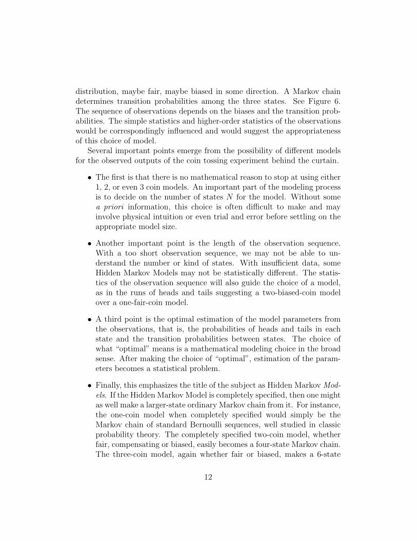
distribution, maybe fair, maybe biased in some direction. A Markov chaindetermines transition probabilities among the three states. See Figure 6.The sequence of observations depends on the biases and the transition prob-abilities. The simple statistics and higher-order statistics of the observationswould be correspondingly influenced and would suggest the appropriatenessof this choice of model.

Several important points emerge from the possibility of different modelsfor the observed outputs of the coin tossing experiment behind the curtain.

• The first is that there is no mathematical reason to stop at using either1, 2, or even 3 coin models. An important part of the modeling processis to decide on the number of states N for the model. Without somea priori information, this choice is often difficult to make and mayinvolve physical intuition or even trial and error before settling on theappropriate model size.

• Another important point is the length of the observation sequence.With a too short observation sequence, we may not be able to un-derstand the number or kind of states. With insufficient data, someHidden Markov Models may not be statistically different. The statis-tics of the observation sequence will also guide the choice of a model,as in the runs of heads and tails suggesting a two-biased-coin modelover a one-fair-coin model.

• A third point is the optimal estimation of the model parameters fromthe observations, that is, the probabilities of heads and tails in eachstate and the transition probabilities between states. The choice ofwhat “optimal” means is a mathematical modeling choice in the broadsense. After making the choice of “optimal”, estimation of the param-eters becomes a statistical problem.

• Finally, this emphasizes the title of the subject as Hidden Markov Mod-els. If the Hidden Markov Model is completely specified, then one mightas well make a larger-state ordinary Markov chain from it. For instance,the one-coin model when completely specified would simply be theMarkov chain of standard Bernoulli sequences, well studied in classicprobability theory. The completely specified two-coin model, whetherfair, compensating or biased, easily becomes a four-state Markov chain.The three-coin model, again whether fair or biased, makes a 6-state

12

Markov chain. In all situations, the classic results of Markov chainswould apply to predict long term averages and stationary distributions,rates of convergence to stationary, and other consequences. Here, theproblem is that we have only the observations or signals, not all thenecessary information. From that, we wish to best determine the un-derlying states and probabilities. The word “best” indicates that wemust consider possible measures of optimality. So this is a modelingand statistical problem, and in some ways an inverse problem. Thataccounts for calling these Hidden Markov Models and not consideringthem from the point of view of Markov chains.

Realistic Hidden Markov Models

CpG Islands

In the human genome the dinucleotide CG (frequently written CpG to dis-tinguish it from the CG base-pair across two strands) is rarer than expectedfrom the independent probabilities of C and G, for reasons of chemistry thattransform the C into a T. For biologically important reasons, the chemicaltransformation is suppressed in short regions of the genome, such as aroundthe promoters or start regions of many genes. In these regions, we see signif-icantly more CpG dinucleotides than elsewhere. Such regions are called CpG

islands. The islands are typically a few hundred to a few thousand baseslong.

Given a short stretch of genomic sequence, how would we decide if itcomes from a CpG island or not? Second, given a long piece of sequence,how would we find the CpG islands in it, if any exist? Here, the Model hastwo states, CpG islands, and non-islands. In each state, the probabilities ofexpressing CpG base-pairs are different.

Profile HMMs in Bioinformatics

For a pair (or more) of proteins, an important question is: How are theproteins similar? The goals are to detect and measure overall similaritybetween protein amino acid sequences, find proteins with similar functionsin different organisms by finding similar subsequences of amino acids called“conserved sequences” and to detect conserved sequences and evolution ofconserved sequences. Alignment is the method for answering these questions.

13

There are two types of alignment: A global alignment is an alignment ofthe full length of two sequences. A local alignment is an alignment of partof one sequence to part of another sequence. For possibly distantly relatedsequences, it might be more sensible to make local alignments of subregionsof high similarity, not the whole sequence. A sample toy alignment is inFigure 7

A C - - A C - T G TT A G A C G G A G C T - T C A C

Figure 7: Toy example of gapped alignment of DNA sequences.

Alignment allows amino acid matches and mismatches along columns withcorresponding scores based on chemistry and biology. In order to make align-ments, we also allow introduction of gaps in either of the protein amino acidsequences. Introducing gaps when making alignments adds penalty scores.

A common task in bioinformatics is to obtain a cluster of related se-quences, e.g. from a database, and then to align those sequences using multi-ple sequence alignment algorithms. The clustering reflects the insights of thebiology community as to which proteins belong within the same family. Theoutcome of the clustering process is a set of distinct protein families. This isthe first step in most phylogenetic analyses. Heuristic algorithms are gener-ally used to create multiple sequence alignments. There are large databasesof proteins and alignments, some created with Hidden Markov Models, someprovide Hidden Markov Model data, see below. An example of an actualmultiple sequence alignment (MSA) is in Figure 8.

A profile HMM (pHMM) is a particular Hidden Markov Model withstates, signals, transition matrix, and emission matrix summarizing a multi-ple sequence alignment. The goal is use this Hidden Markov Model informa-tion about the MSA to align a new query sequence. Profile HMMs have threestates for each alignment position, i.e. each column in the multiple sequencealignment. Three outcomes are possible when aligning each residue of thequery sequence with the MSA:

• the query residue may align (match) with the next residue of the MSA;

• it may correspond to an insertion (new residue) relative to the MSA;and

14

Figure 8: Alignment of acidic ribosomal protein P0 from several organisms.

15

• it may correspond to a deletion (a gap) relative to the MSA.

There are heuristic rules assigning MSA columns as match states, for exam-ple, the MSA has a match column if less than half of the characters are gaps.The length of a pHMM is the number of columns in the MSA assigned tomatch states. Each match state in the pHMM has its corresponding set ofemission probabilities, generated from counting the frequencies of each aminoacid in the corresponding column. Insertions, i.e. portions of the query se-quence that do not match anything in the multiple alignment, correspondto an insert state. As in the case of the match states, each insert state hasits own set of emission probabilities. The insert state emission probabilitiesare typically generated using the distribution of amino acids over the entireMSA. A delete state is possible for each of the positions in the MSA. Thedelete state is an example of a silent state in the model, as it does not emitany residues.

Let l denote the number of match locations. Then the associated profileHMM has 3l + 3 states in the underlying Markov process, namely:

• a “start” state S;

• an “end” state E;

• l match states M1, . . . ,Ml;

• l “delete” states D1, . . . , Dl; and

• and l + 1 “insert” states I0, . . . Il.

Figure 9: Schematic diagram of the transitions in a profile HMM

16

Thus, a pHMM typically has many more states than the previous examplesof Hidden Markov Models with only a handful of states. The connectionsbetween the states is highly structured and more complicated than the otherexamples of Hidden Markov Models. The set of emissions, 20 or fewer, isabout the same order of magnitude as in the other examples.

A typical application of a profile HMM is the following: Start with collec-tion of protein families (clusters) F1 . . . Fk, where all proteins within a familyhave the same length after assigning gaps as necessary. For each family Fi,construct a corresponding profile HMM, λ(Fi) in the notation of the nextsection. The objective is to assign a newly sequenced protein to one of thek families. Then compute the likelihood P [O |λ(Fi)] of the gap-aligned newprotein for each of the k profile HMMs. The new protein is then assignedto the family for which the likelihood is maximum. This is the “scoring”problem of Hidden Markov Models.

Language Analysis Translation

Language translation is a classic application of Hidden Markov Models, orig-inating with Cave and Neuwirth, see [4] for history and additional details.Suppose you do not understand English, but you do know something aboutpunctuation. You obtain a large body of English text, such as the “BrownCorpus”. Henry Kucera and W. Nelson Francis at Brown University compiledThe Brown University Standard Corpus of Present-Day American English asa general corpus (text collection) in the field of corpus linguistics. The BrownCorpus contains 500 samples of English-language text, totaling roughly onemillion words, compiled from works published in the United States in 1961.The Brown Corpus is one of many such corpuses, available through the Nat-ural Language Toolkit, see nltk.org. With knowledge of Hidden MarkovModels, but no knowledge of English, you would like to determine somebasic properties of this mysterious writing system. Can you partition thecharacters into sets so that characters in each set are “different” in somestatistically significant way?

First remove all punctuation and numbers and convert all letters to lowercase. This leaves 26 distinct letters and the space, for a total of 27 symbols.The observations are the series of characters found in the resulting text.Then test the hypothesis that English text has an underlying Markov chainwith two states. For each of these two hidden states, assume that the 27symbols appear according to a fixed probability distribution. This sets up a

17

Hidden Markov Model with N = 2 and M = 27 where the state transitionprobabilities and the observation probabilities from each state are unknown.

Results of a case study, [4] using the first 50,000 observations from theBrown Corpus of letters converted to lower case and the space are in Table 2.Without having any assumption about the nature of the two states, theresults sort into two familiar categories! The probabilities tell us that theone hidden state contains the vowels while the other hidden state contains theconsonants. Interestingly, space is more like a vowel and “y” is a consonant.The Hidden Markov Model “deduces” the statistically significant differencebetween vowels and consonants without knowing anything about the Englishlanguage.

Cave and Neuwirth obtain further results by allowing more than twohidden states. They are able to obtain and sensibly interpret the results formodels with up to 12 hidden states. This example has further applicationsto automatic language translation.

This example suggests Hidden Markov Models may be applicable to crypt-analysis. In fact, a Hidden Markov Model has been applied to “secret mes-sages” such as Hamptonese, the Voynich Manuscript and the “Kryptos”sculpture at the CIA headquarters but without too much success, [4]. Partlythe reasons for success or failure depend on the quality of the transcriptionsand partly on the assumptions that the cipher text is a plaintext in an un-known language, and not steganography, or even just babbling (glossolalia).

Speech Recognition

A classic example and practical application of Hidden Markov Models isspeech recognition, especially isolated word recognition. Hidden MarkovModels were developed in the 1960s and 1970s for satellite communication.Andrew Viterbi made a key contribution to the theory in 1967. They werelater adapted for language analysis, translation and speech recognition inthe 1970s and 1980s by Bell Labs and IBM [2]. Interest in HMMs for speechrecognition seems to have peaked in the late 1980s.

Speech recognition takes place in several steps:

1. Feature analysis – a spectral or temporal analysis of the speech signalto decompose the continuous sound sample into discrete observationsof speech sounds for the Hidden Markov Model.

18

State 0 State 1a 0.13845 0.00075b 0.00000 0.02311c 0.00062 0.05614d 0.00000 0.06937e 0.21404 0.00000f 0.00000 0.03559g 0.00081 0.02724h 0.00066 0.07278i 0.12275 0.00000j 0.00000 0.00365k 0.00182 0.00703l 0.00049 0.07231

m 0.00000 0.03889n 0.00000 0.11461o 0.13156 0.00000p 0.00040 0.03674q 0.00000 0.00153r 0.00000 0.10225s 0.00000 0.11042t 0.01102 0.14392u 0.04508 0.00000v 0.00000 0.01621w 0.00000 0.02303x 0.00000 0.00447y 0.00019 0.02587z 0.00000 0.00110

space 0.33211 0.01298

Table 2: Emission probabilities of letters from the two states, from [4]

19

2. Unit matching – the speech signal parts are matched to words orphonemes with a Hidden Markov Model.

3. Lexical analysis – if the units are phonemes, combine the units into rec-ognized words with either a deterministic or a probabilistic finite statenetwork. If the units are words, this step can generally be eliminated.

4. Syntactic analysis – with a grammar, group words into proper se-quences. If single word like “yes” or “no”, or digit sequences, thisstep is minimal or completely eliminated.

5. Semantic analysis – interpret the words or word sequences for the taskmodel.

Concentrating on the second step of unit matching, assume we have avocabulary of V words to recognize. We have a training set of L tokensof each word. We also have an independent observation set. We use theobservations from the set of L tokens to estimate the optimum parametersfor each word, creating model λv for the vth vocabulary word, 1 ≤ v ≤ V .For each unknown word in the observation sequence O = O0O1 . . .OT−1 andfor each word model λv we calculate Pv = P [O |λv]. We choose the wordwhose model probability is highest

v? = argmax1≤v≤V

[Pv].

For example, we could train an Hidden Markov Model, say λ0 to recognizethe spoken word “no” and train another Hidden Markov Model, say λ1 torecognize the spoken word “yes”. (This is the step we will later call thesolution to Problem 3.) Then given an unknown spoken word, we can usethe Hidden Markov Model to score this word against λ0 and also againstλ1 to decide if the spoken word is more likely “no”, “yes” or neither. (Thisis the problem we will later call Problem 1.) Notice that this applicationdoes not uncover the hidden states (which we will later call Problem 2) butsuch information might provide additional insight into the underlying speechmodel.

The Hidden Markov Model for speech recognition is very efficient. Forisolated word recognition with the Viterbi Algorithm, a vocabulary of V =100 words with an N = 5 state model, and 40 observations, it takes about105 computations (additions/multiplications) for a single word recognition.

20

It is hard to determine what current (2017) speech recognition applica-tions are based on. Explanations are clouded with buzzwords and hype, withno theory. Common buzzwords surrounding current (2017) speech recog-nition are “artificial intelligence”, “machine learning”, “neural networks”,and “deep learning”, but there does not seem to be a connection to HiddenMarkov Models.

Sources

The variable factory example is adapted from Sheldon M. Ross, Introductionto Probability Models, Section 4.11, pages 256-262, Academic Press, 2006,9th Edition.

The paleontological temperature model is adapted from “A RevealingIntroduction to Hidden Markov Models”, by Mark Stamp.

The cheating casino and CpG Islands example is adapted from BiologicalSequence Analysis, by R. Durbin, S. Eddy, A. Krogh, and G. Mitchison,Chapter 3, pages 46-79.

The urn and ball model is adapted from “An Introduction to HiddenMarkov Models”, by L.R. Rabiner and B. H. Juang, 1986.

The language analysis example is adapted from “A Revealing Introduc-tion to Hidden Markov Models”, by Mark Stamp.

The speech recognition example is adapted from “A Tutorial on HiddenMarkov Models and Selected Applications in Speech Recognition” by L. R.Rabiner.

Algorithms, Scripts, Simulations

Algorithm

Scripts

21

Problems to Work for Understanding

1.

2.

3.

4.

Reading Suggestion:

References

[1] L. R. Rabiner and B. H. Juang. An Introduction to Hidden MarkovModels. IEEE ASSP Magazine, pages 4–16, January 1986. hidden markovmodels.

[2] Lawrence R. Rabiner. A Tutorial on Hidden Markov Models and SelectedApplications in Speech Recognition. Proceedings of the IEEE, 77(3):257–286, February 1989. hidden Markov model, speech recognition.

[3] Sheldon M. Ross. Introduction to Probability Models. Academic Press,9th edition, 2006.

[4] Mark Stamp. A revealing introduction to hidden markov models.https://www.cs.sjsu.edu/ stamp/RUA/HMM.pdf, December 2015.

22

Outside Readings and Links:

1.

2.

3.

4.

I check all the information on each page for correctness and typographicalerrors. Nevertheless, some errors may occur and I would be grateful if you wouldalert me to such errors. I make every reasonable effort to present current andaccurate information for public use, however I do not guarantee the accuracy ortimeliness of information on this website. Your use of the information from thiswebsite is strictly voluntary and at your risk.

I have checked the links to external sites for usefulness. Links to externalwebsites are provided as a convenience. I do not endorse, control, monitor, orguarantee the information contained in any external website. I don’t guaranteethat the links are active at all times. Use the links here with the same caution asyou would all information on the Internet. This website reflects the thoughts, in-terests and opinions of its author. They do not explicitly represent official positionsor policies of my employer.

Information on this website is subject to change without notice.

Steve Dunbar’s Home Page, http://www.math.unl.edu/~sdunbar1Email to Steve Dunbar, sdunbar1 at unl dot edu

Last modified: Processed from LATEX source on April 12, 2017

23