Embed Size (px)
DESCRIPTION
Topics in Space Weather Lecture 12. Ionosphere. Robert R. Meier School of Computational Sciences George Mason University [email protected] CSI 769 22 November 2005. Topics. Photoionization & Photoelectrons Photoionization & Chapman Layer Ionospheric Layers F-Region E-Region D-Region - PowerPoint PPT Presentation
Citation preview
1
Topics in Space WeatherTopics in Space Weather
Lecture 12
Topics in Space WeatherTopics in Space Weather
Lecture 12
Ionosphere
Robert R. Meier
School of Computational SciencesGeorge Mason University
CSI 76922 November 2005
2
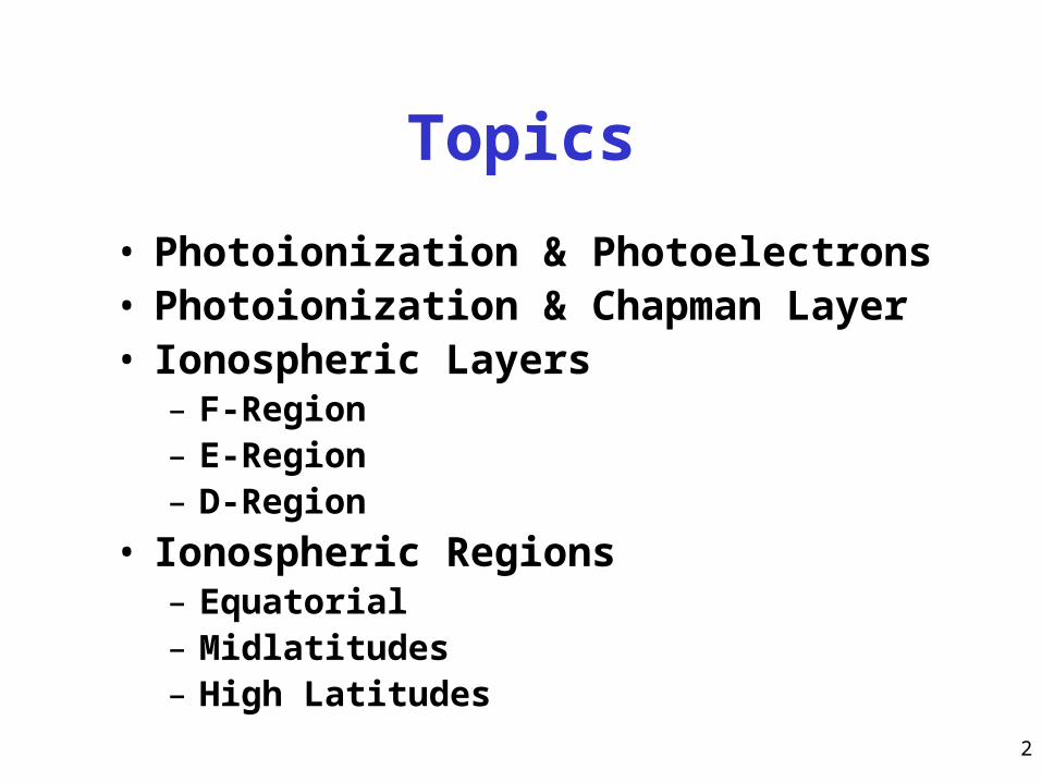
Topics
• Photoionization & Photoelectrons• Photoionization & Chapman Layer• Ionospheric Layers
– F-Region– E-Region– D-Region
• Ionospheric Regions– Equatorial– Midlatitudes– High Latitudes

3

4
Photoionization and Photoelectrons
• Important source of–Secondary ionization–Dayglow emissions
• Heat source for plasmasphere• Conjugate photoelectrons important• Concepts analogous to auroral electron precipitation

5
Photoionization
Processes– O + h ( 91.0 nm) O+ + e– O2 + h ( 102.8 nm) O2
+ + e– N2 + h ( 79.6 nm) N2
+ + e
Ionization Energies
Species Dissociation
(Å)
Dissociation
(eV)
Ionization
(Å)
Ionization
(eV)
O
O2
N2
2423.7
1270.4
5.11
9.76
910.44
1027.8
796
13.62
12.06
15.57
6
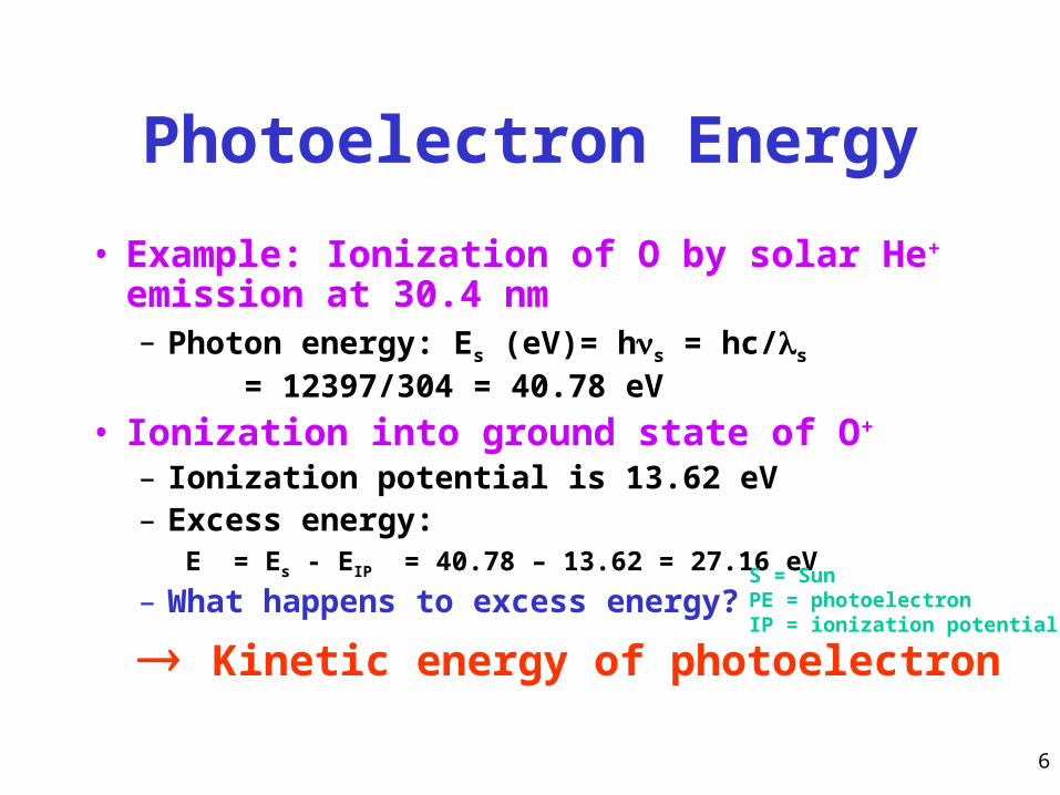
Photoelectron Energy
• Example: Ionization of O by solar He+ emission at 30.4 nm– Photon energy: Es (eV)= hs = hc/s
= 12397/304 = 40.78 eV
• Ionization into ground state of O+
– Ionization potential is 13.62 eV– Excess energy:
E = Es - EIP = 40.78 – 13.62 = 27.16 eV
– What happens to excess energy?
Kinetic energy of photoelectron
S = SunPE = photoelectronIP = ionization potential
7
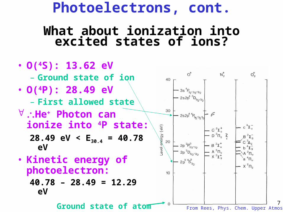
Photoelectrons, cont.
What about ionization into excited states of ions?
• O(4S): 13.62 eV– Ground state of ion
• O(4P): 28.49 eV– First allowed state
He+ Photon can ionize into 4P state:28.49 eV < E30.4 = 40.78 eV
• Kinetic energy of photoelectron:40.78 – 28.49 = 12.29 eV
Ground state of atom From Rees, Phys. Chem. Upper Atmos.

8
Photoelectrons, cont.
• Photoelectrons produced when O+ is in the ground state have sufficient energy to ionize O– EPE = 28.49 eV > 13.62 eV (ionization potential
of O)– Note that if O+ is in the 4P state, the excess
energy is 12.29 eV• Not sufficient to ionize N2 or O, but is for O2
• Therefore photoelectrons are an important source of secondary ionization– ~25% at higher altitudes– More at lower altitudes where X-rays can
produce very energetic photoelectrons
9
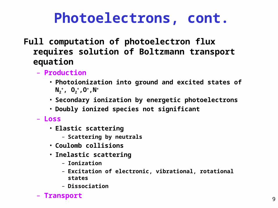
Photoelectrons, cont.
Full computation of photoelectron flux requires solution of Boltzmann transport equation– Production
• Photoionization into ground and excited states of N2+,
O2+,O+,N+
• Secondary ionization by energetic photoelectrons
• Doubly ionized species not significant
– Loss• Elastic scattering
– Scattering by neutrals
• Coulomb collisions
• Inelastic scattering– Ionization – Excitation of electronic, vibrational, rotational states– Dissociation
– Transport
10
Photoelectrons, cont.
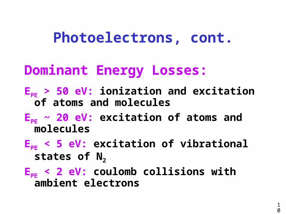
Dominant Energy Losses:
EPE > 50 eV: ionization and excitation of atoms and molecules
EPE ~ 20 eV: excitation of atoms and molecules
EPE < 5 eV: excitation of vibrational states of N2
EPE < 2 eV: coulomb collisions with ambient electrons
11
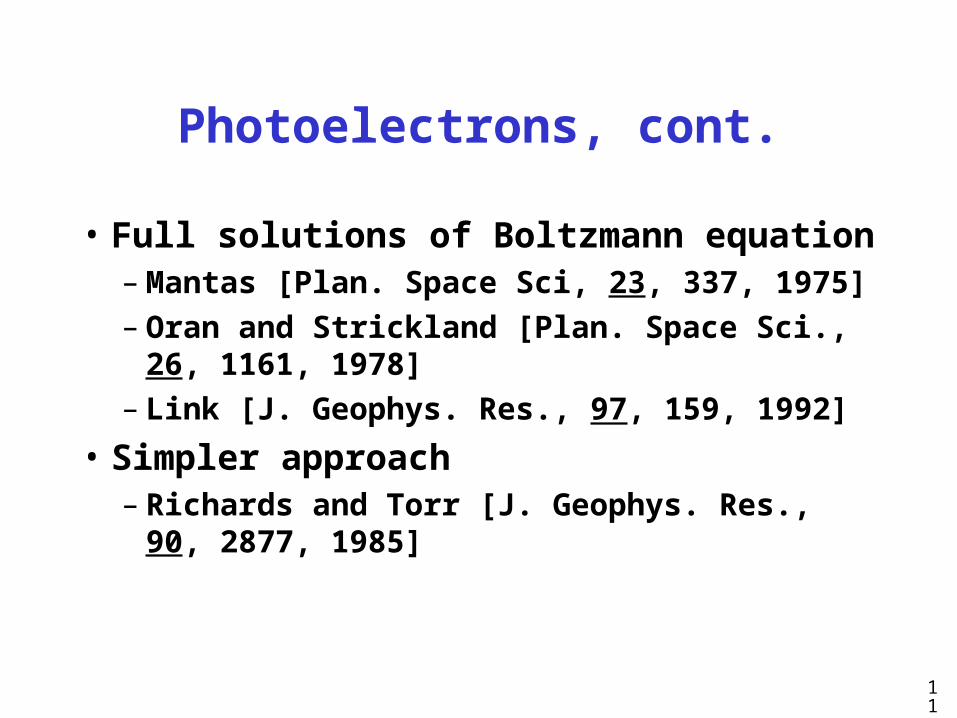
Photoelectrons, cont.
• Full solutions of Boltzmann equation– Mantas [Plan. Space Sci, 23, 337, 1975]– Oran and Strickland [Plan. Space Sci.,
26, 1161, 1978]– Link [J. Geophys. Res., 97, 159, 1992]
• Simpler approach– Richards and Torr [J. Geophys. Res., 90,
2877, 1985]
12
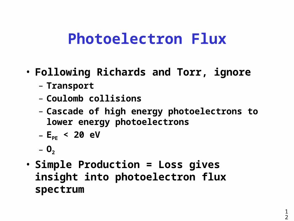
Photoelectron Flux
• Following Richards and Torr, ignore– Transport– Coulomb collisions– Cascade of high energy photoelectrons to
lower energy photoelectrons
– EPE < 20 eV
– O2
• Simple Production = Loss gives insight into photoelectron flux spectrum
13
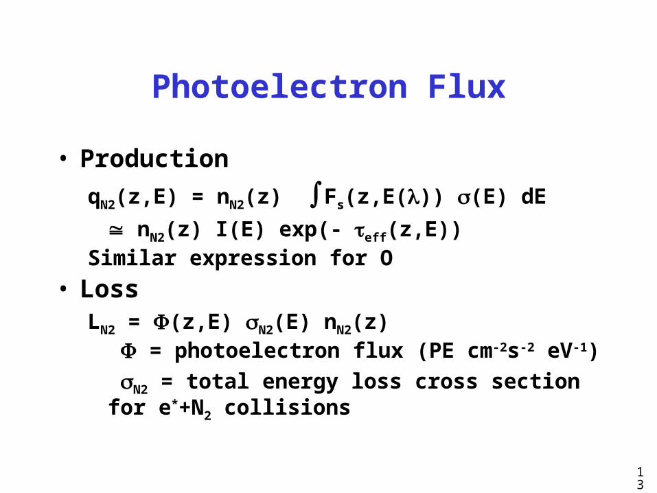
Photoelectron Flux
• Production
qN2(z,E) = nN2(z) Fs(z,E()) (E) dE
nN2(z) I(E) exp(- eff(z,E))
Similar expression for O
• LossLN2 = (z,E) N2(E) nN2(z)
= photoelectron flux (PE cm-2s-2 eV-1)
N2 = total energy loss cross section for e*+N2 collisions
14
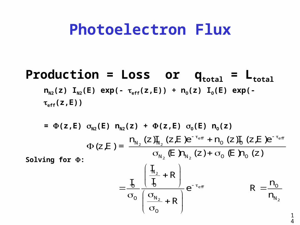
Photoelectron Flux
Production = Loss or qtotal = Ltotal
nN2(z) IN2(E) exp(- eff(z,E)) + nO(z) IO(E) exp(- eff(z,E))
= (z,E) N2(E) nN2(z) + (z,E) O(E) nO(z)
Solving for :
eff eff
2 2
2 2
2
eff
2 2
N N O O
N N O O
N
OO O
NO N
O
n (z)I (z,E)e n (z)I (z,E)e(z,E) =
(E)n (z) (E)n (z)
IR
II ne R
nR
15
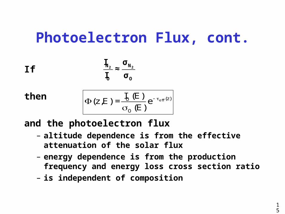
Photoelectron Flux, cont.
If
then
and the photoelectron flux – altitude dependence is from the effective
attenuation of the solar flux
– energy dependence is from the production frequency and energy loss cross section ratio
– is independent of composition
2 2N N
O O
I σ≈
I σ
eff (z)O
O
I (E)(z,E) = e
(E)

16
Photoelectron Flux, cont.
Simple and full PE flux calculations
Some differences < 20 eV and > 50 eV
Richards and Torr [1983]

17
Photoelectron Flux, cont.
Simple and full PE flux calculations
Compare with AE-E PE measurements
Richards and Torr [1983]
18
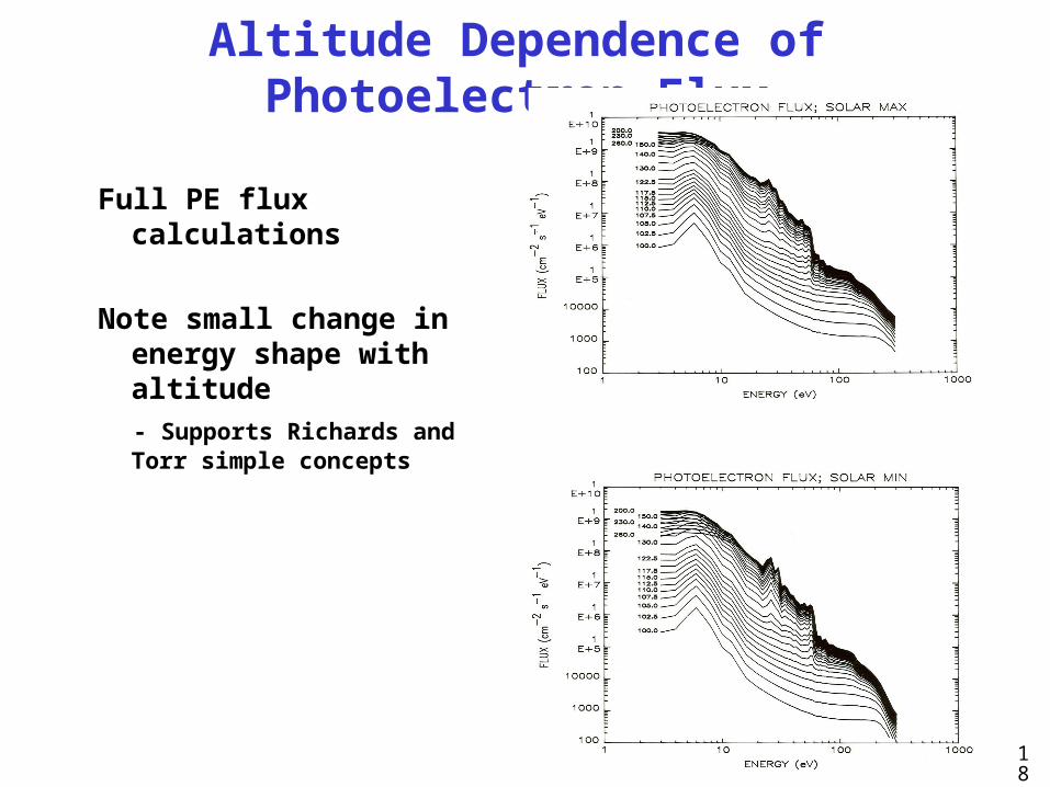
Altitude Dependence of Photoelectron Flux
Full PE flux calculations
Note small change in energy shape with altitude
- Supports Richards and Torr simple concepts
19
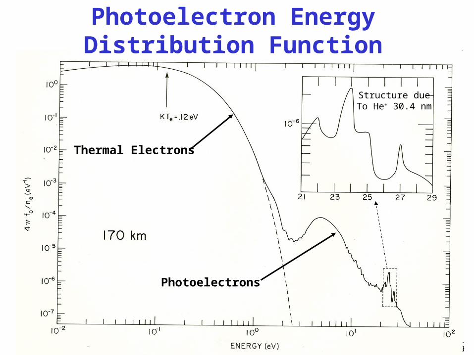
Photoelectron Energy Distribution Function
Thermal Electrons
Photoelectrons
Structure dueTo He+ 30.4 nm
20
Photoionization and Photoionization and the Classic Chapman the Classic Chapman
IonosphereIonosphere
21
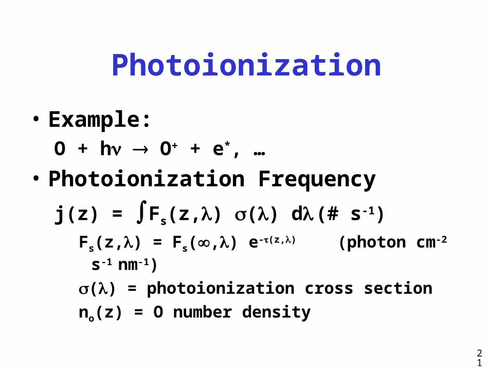
Photoionization
• Example:O + h O+ + e*, …
• Photoionization Frequency
j(z) = Fs(z,) () d (# s-1)
Fs(z,) = Fs(,) e-(z,)(photon cm-2 s-1 nm-1)
() = photoionization cross section
no(z) = O number density

22
Photoionization Rate
• q(z) = no(z) j(z) (# cm-3 s-1)– no(z) = O number density
• Assume single constituent, isothermal atmosphere, photoionized by a single wavelength emission:
n(z) = no(z) = no(zo) e-(z-zo)/H
q(z) = no(zo) e-(z-zo)/H Fs(,) e-(z,)

23
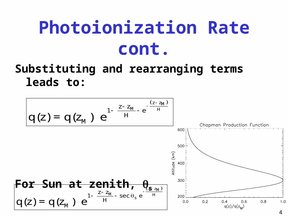
Photoionization Rate cont.
o
z zooH
o
z zoo H
o
z z
Ho
z
z-z- n(z )HeH
o s
z zn(z )He
H
o s
(z) n(z ')dz ' n(z )He
q(z) = n(z ) e F ( ) e
q(z) = n(z ) F ( ) e
Peak in layer occurs when
Working through, this occurs at
)Mdq(z
0dz
M oz z
HM o(z ) 1 n(z )He
24
Photoionization Rate cont.
Substituting and rearranging terms leads to:
For Sun at zenith, s
z zM
M Hz z1 e
HMq(z) = q(z ) e
z zM
M Hs
z z1 sec e
HMq(z) = q(z ) e
25
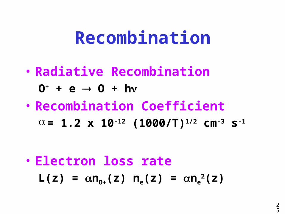
Recombination
• Radiative Recombination O+ + e O + h
• Recombination Coefficient= 1.2 x 10⁻¹² (1000/T)1/2 cm-3 s-1
• Electron loss rateL(z) = nO+(z) ne(z) = ne
2(z)
26
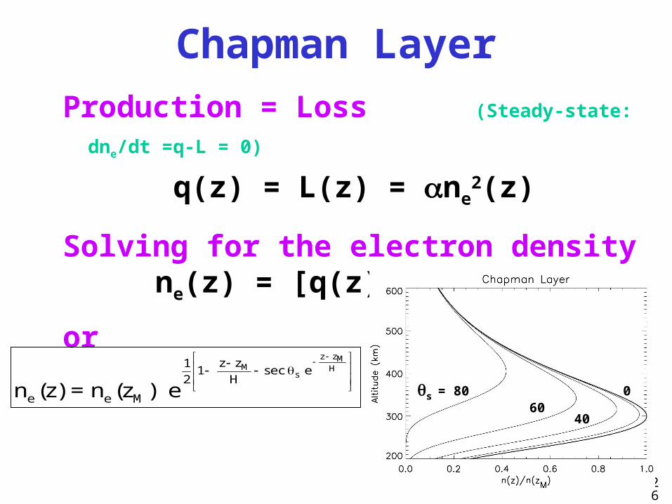
Chapman Layer
Production = Loss (Steady-state: dne/dt =q-L = 0)
q(z) = L(z) = ne2(z)
Solving for the electron densityne(z) = [q(z) / ]1/2
or
z zMM H
sz z1
1 sec e2 H
e e Mn (z) = n (z ) e s = 8060
40
0
27
Ionospheric LayersIonospheric Layers• D-Region• E - region• F1 – Region• F2 – Region• Plasmasphere

28
29
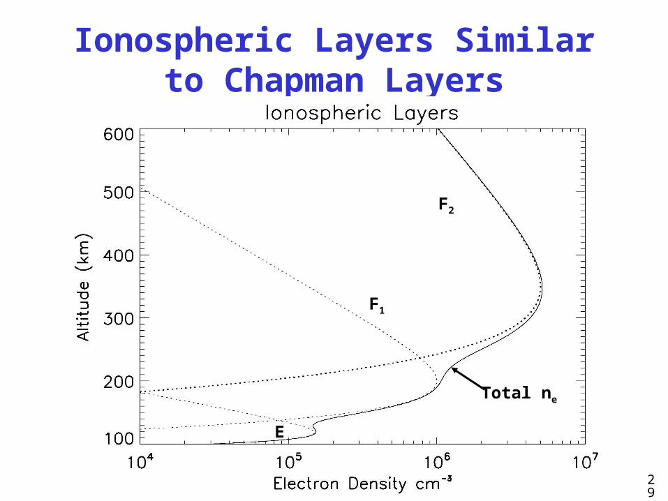
Ionospheric Layers Similar to Chapman Layers
F2
F1
E
Total ne
30
D-Region
• Ugly ion chemistry• See:
– Turunen, E., H. Matveinen, J. Tolvanen, and H. Ranta, D-region ion chemistry model, in STEP Handbook of Ionospheric Models, R. W. Schunk (ed.), pp. 1-25, 1996.
– Torkar, K. M., and M. Friedrich, Tests of an ion-chemical model of the D- and lower E-region, J. Atm. Terr. Phys., 45, 369-385, 1983.
• Tens of species—some models have more• Few measurements
– Requires rockets
31
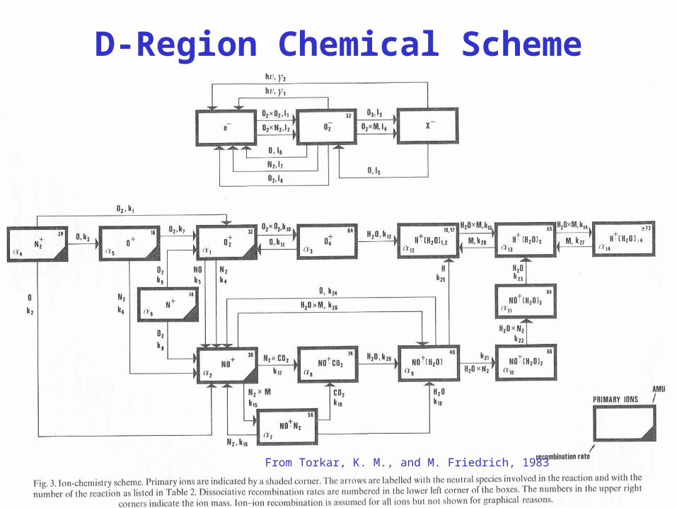
D-Region Chemical Scheme
From Torkar, K. M., and M. Friedrich, 1983
32
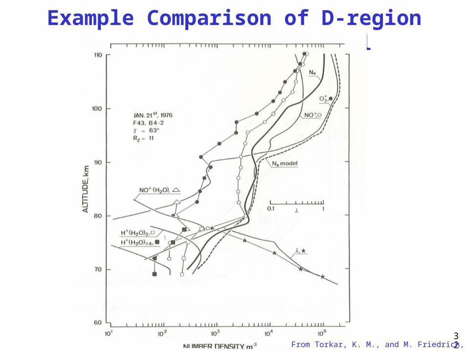
Example Comparison of D-region Observations and Model
From Torkar, K. M., and M. Friedrich, 1983

33
E-region
• Production--photoionizationO2 + h O2
+ + e j = photoionzation rate
N2 + h N2+ + e
O + h O+ + e (smaller)
• Chemistry– N2
+ + O NO+ + N or O+ + N2
– O+ + N2 NO+ + N
• Loss—Dissociative Recombination– NO+ + e N + O
– O2+ + e O + O kO2+ = recombination rate
• Net Result:– Major ions in E region are O2
+ and NO+
– To first order, diffusion & dynamics slow compared with photochemistry
34
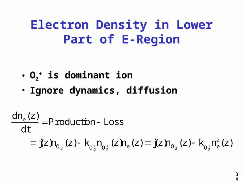
Electron Density in Lower Part of E-Region
• O2+ is dominant ion
• Ignore dynamics, diffusion
2 22 2 2
e
2O e O eO O O
dn (z)Pr oduction Loss
dt
j(z)n (z) k n (z)n (z) j(z)n (z) k n (z)
35
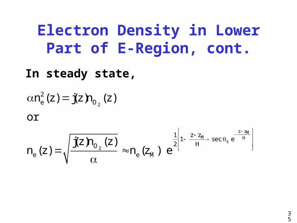
Electron Density in Lower Part of E-Region, cont.
In steady state,
2
z zMM H
s
2
2e O
z z11 sec e
2 HOe e M
n (z) j(z)n (z)
or
j(z)n (z)n (z) n (z ) e

36
Recombination Rates and Electron Lifetimes
Lower E-Region• O2
+ + e O + O kO2+ = 1.9 x 10⁻⁷ (Te/300)-0.5 cm3s-1
• nO2+ ~ 105 cm-3 & Te ~ Tn = 300K at ~ 110 km• Rate = kO2+ nO2+ = 0.019 s-1
• Lifetime = 1/Rate = 53 s
Upper E-Region• NO+ + e N + O kNO+ ~ 4.2 x 10⁻⁷ (Te/300)-0.85 cm3s-1
• nNO+ ~ 105 cm-3 & Te ~ Tn = 587K at ~ 140 km• Rate = kNO+ nNO+ = 0.024 s-1
• Lifetime = 1/Rate = 42 s
37
F1-Region
• Similar to E-region
• Must include O+, the dominant ion
• Diffusion begins to be important
38
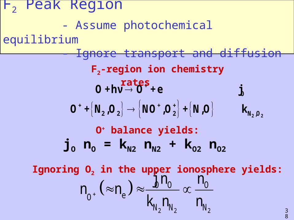
F2 Peak Region - Assume photochemical equilibrium - Ignore transport and diffusion
2 2
+O
+ + +2 2 2 N ,O
O +hν O +e j
O + N ,O NO ,O + N,O k
O+ balance yields:
jO nO = kN2 nN2 + kO2 nO2
2 2 2
O O OeO
N N N
j n nn n
k n n
F2-region ion chemistry rates
Ignoring O2 in the upper ionosphere yields:
39
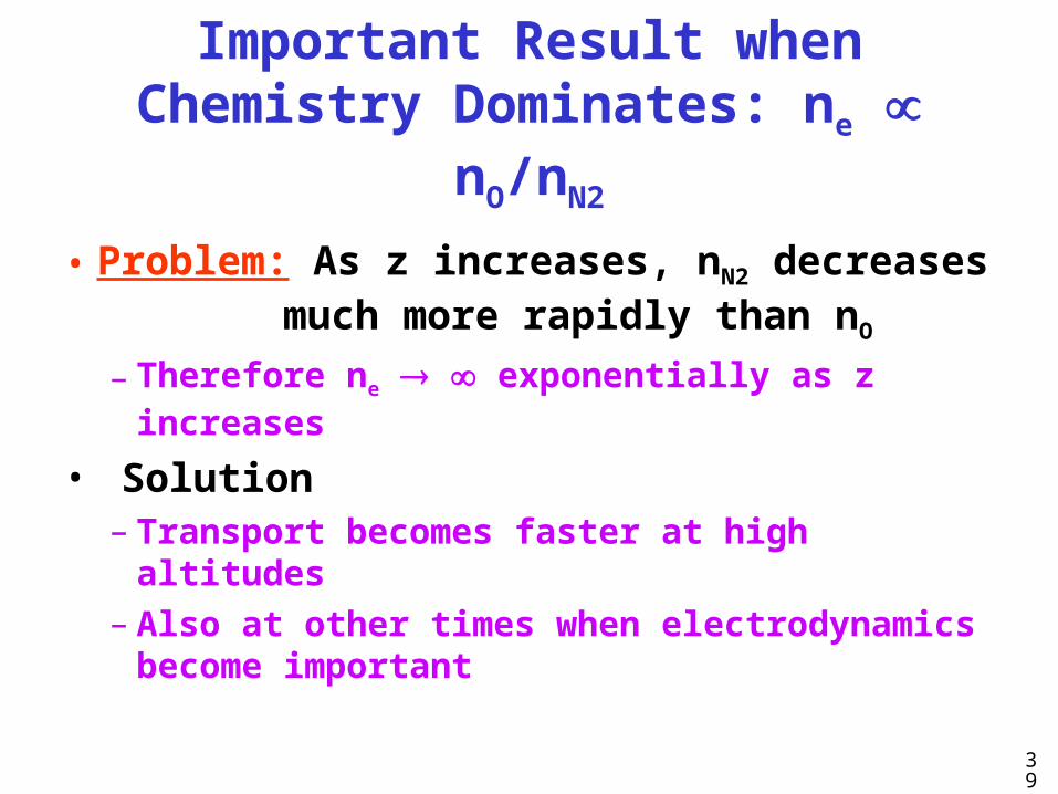
Important Result when Chemistry Dominates: ne nO/nN2
• Problem: As z increases, nN2 decreases much more rapidly than nO
– Therefore ne exponentially as z increases
• Solution– Transport becomes faster at high altitudes– Also at other times when electrodynamics
become important

40
Recombination Rates and Electron Lifetimes in F-Region
• Production: O + h O+ + e– Rate = j = 2 – 6 x 10⁻⁷ s-1
– Lifetime = 5 – 1.6 x 10⁶ s ( 58 - 19 days)
• Intermediate step: O+ + N2 NO+ + N– (or O2)– Rate for N2: kN2 nN2 = 10-12cm3s-1 5.5x108cm-3 = 5.5 x 10⁻⁴ s-1
– Lifetime = 1800 s
• Loss: NO+ + e N + O– ne ~ 106 cm-3 & Te ~ 1800K at ~ 250 km– Rate = kNO+ ne = 0.129 s-1
– Lifetime = 1/Rate = 7.8 s
• Loss: O+ + e O– ne ~ 106 cm-3 & Te ~ 1400K at ~ 250 km– Rate = kO+ ne = 1.2x10⁻¹² (1000/T)0.5 x ne s-1 = 1 x 10⁻⁶s– Lifetime = 1/Rate = 106 s = 11 days
41
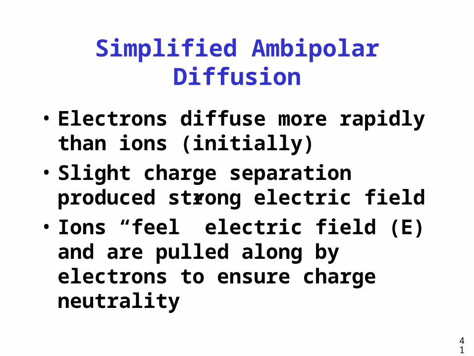
Simplified Ambipolar Diffusion
• Electrons diffuse more rapidly than ions (initially)
• Slight charge separation produced strong electric field
• Ions “feel” electric field (E) and are pulled along by electrons to ensure charge neutrality

42
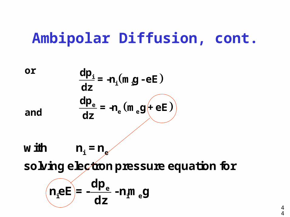
Ambipolar Diffusion, cont.
• Again, diffusive equilibrium– net diffusion velocity is zero– Ignore ion chemistry
• Assume plasma flow parallel to magnetic field lines – taken to be vertical (upper mid to high
latitudes)
• Assume single ion species– Same as neutral species– Note: can be generalized to multiple ions

43
Ambipolar Diffusion, cont.
• Force on ions and electrons:Fi = eE (upward pull)
Fe = - eE (downward pull)
• Force balance for ions and electrons in slab of area, A:Ions: dpi A = - ni mi g Adz + ni eE Adz
Electrons: dpe A = - ne me g Adz - ne eE Adz
44
Ambipolar Diffusion, cont.
or
and
ii i
ee e
dp=-n mg-eE
dzdp
=-n mg+eEdz
i e
ei i e
with n = n
solving electron pressure equation for
dpn eE = - - nm g
dz

45
Ambipolar Diffusion, cont.
i i i e
e i
nkT and nkT
1
T H
e eii i i e i i
i ei i
i e
i i i
i
dp dpdp=-nmg-nmg- -nmg-
substitutingintoionpressu
dz dz dzd p +p
=-nmgdz
p p
d
reequatio
n nmg=-
d
n
z k T
:
Since
Gombosi, Equation 10.48
46
Ambipolar Diffusion, cont.
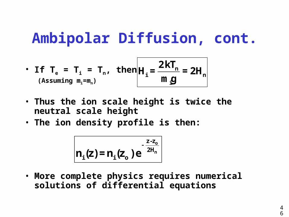
• If Te = Ti = Tn, then(Assuming mi=mn)
• Thus the ion scale height is twice the neutral scale height
• The ion density profile is then:
• More complete physics requires numerical solutions of differential equations
ni n
i
2kTH = =2H
mg
o
n
z-z
2Hi i on (z) = n (z ) e
47
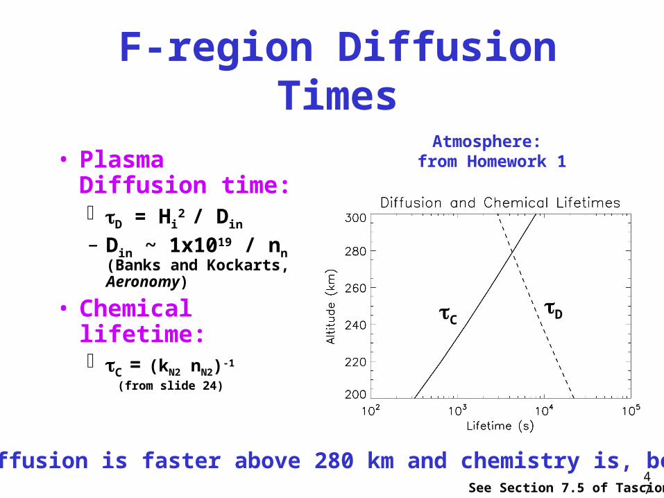
F-region Diffusion Times
• Plasma Diffusion time: D = Hi
2 / Din
– Din ~ 1x10¹⁹ / nn (Banks and Kockarts, Aeronomy)
• Chemical lifetime: C = (kN2 nN2)-1
(from slide 24)
CD
Atmosphere: from Homework 1
Diffusion is faster above 280 km and chemistry is, belowSee Section 7.5 of Tascione
48
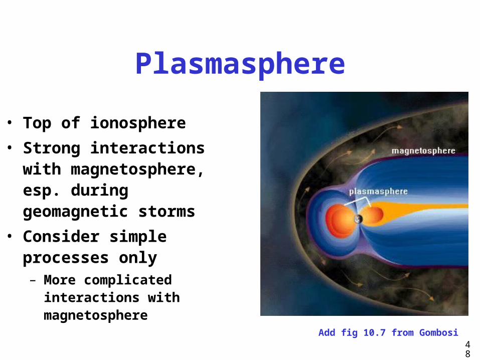
Plasmasphere
• Top of ionosphere
• Strong interactions with magnetosphere, esp. during geomagnetic storms
• Consider simple processes only– More complicated interactions
with magnetosphere
Add fig 10.7 from Gombosi
49
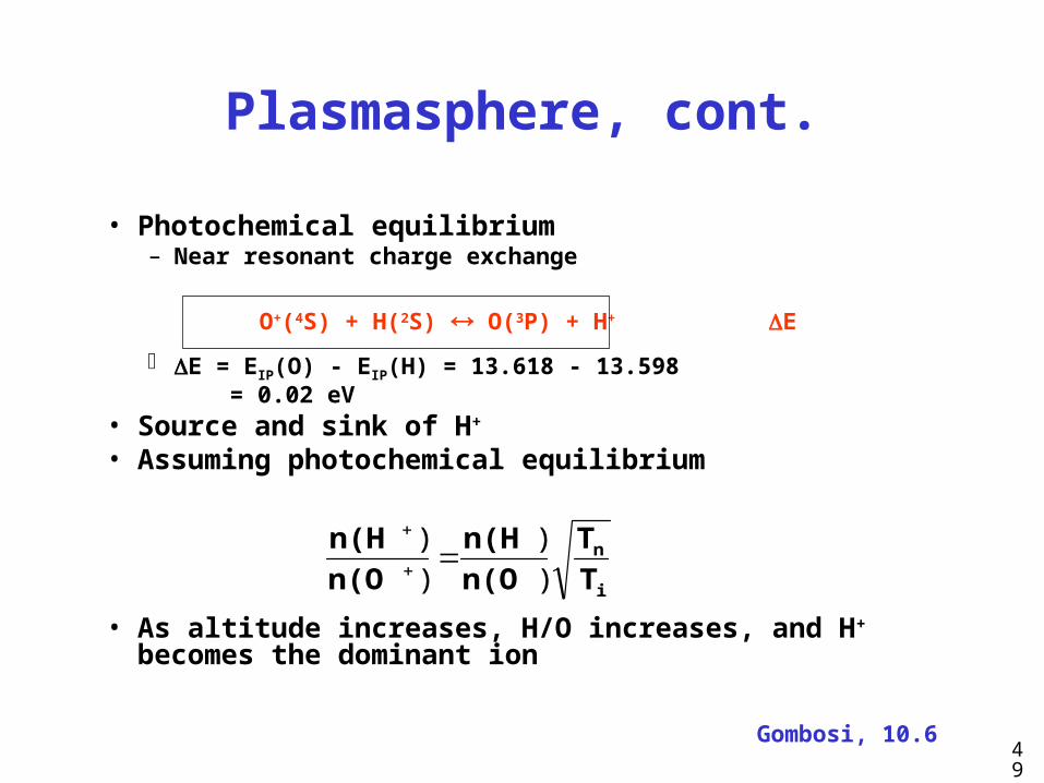
• Photochemical equilibrium– Near resonant charge exchange
O+(4S) + H(2S) O(3P) + H+ E
E = EIP(O) - EIP(H) = 13.618 - 13.598 = 0.02 eV
• Source and sink of H+
• Assuming photochemical equilibrium
• As altitude increases, H/O increases, and H+ becomes the dominant ion
Plasmasphere, cont.
i
n
TT
n(On(H
n(On(H
)
)
)
)
Gombosi, 10.6

50
Plasmasphere, cont.
• He+ is second most populous ion– Tracks He+
• Can image plasmasphere by observing resonant scattering of solar He+ 30.4 nm emission line
He+(2S)+ h30.4 He+ (2P)
He+(2S)+ h30.4
From IMAGE SatelliteSun
51
Ionospheric RegionsIonospheric Regions
Low LatitudesLow LatitudesMid LatitudesMid LatitudesHigh LatitudesHigh Latitudes
52
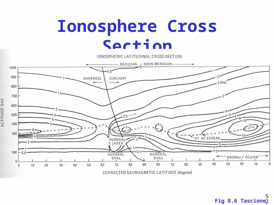
Ionosphere Cross Section
Fig 8.6 Tascione
53
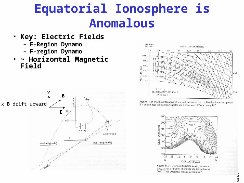
Equatorial Ionosphere is Anomalous
• Key: Electric Fields– E-Region Dynamo– F-region Dynamo
• ~ Horizontal Magnetic Field
E x B drift upward
vB
E
54
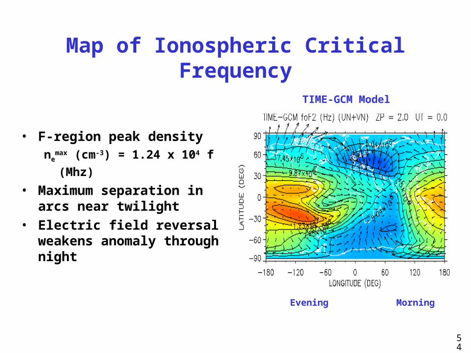
Map of Ionospheric Critical Frequency
• F-region peak density
nemax (cm-3) = 1.24 x 10⁴ f (Mhz)
• Maximum separation in arcs near twilight
• Electric field reversal weakens anomaly through night
TIME-GCM Model
Evening Morning
55
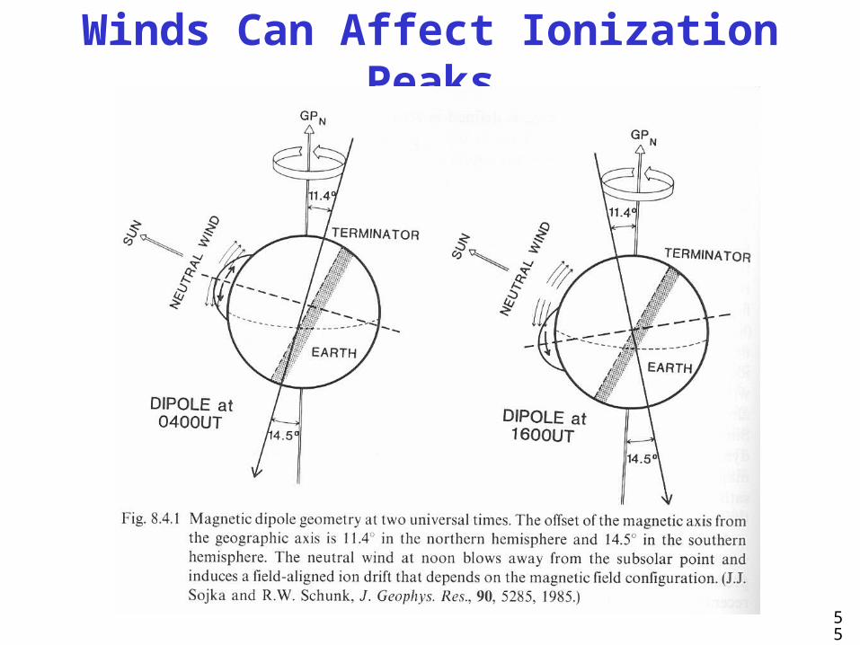
Winds Can Affect Ionization Peaks
56
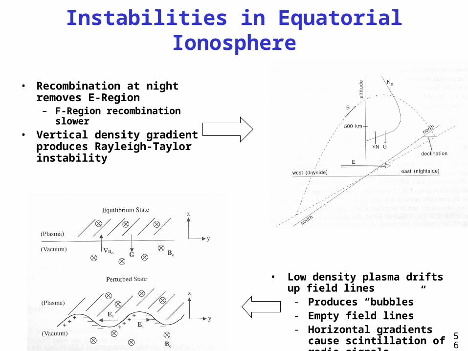
Instabilities in Equatorial Ionosphere
• Recombination at night removes E-Region
– F-Region recombination slower
• Vertical density gradient produces Rayleigh-Taylor instability
• Low density plasma drifts up field lines
- Produces “bubbles”- Empty field lines- Horizontal gradients cause
scintillation of radio signals

57
GUVI FUV Ionosphere Observations
Longitude
Latit
ude
Depleted Flux Tubes
e + O+ O* (135 nm) I = ne2 ds
9/22/2002
e + O+ O* (135 nm)
Equ
ator
ial A
nom
aly
Magnetic Equator

58
18MidnightNoon
Solar Maximum
Noon Midnight18
Solar Minimum
20dB
15dB10dB
5dB2dB
1dB
L-Band
SOLAR CYCLE CHANGES INDUCE SOLAR CYCLE CHANGES INDUCE IONOSPHERIC IRREGULARITIES THAT AFFECT IONOSPHERIC IRREGULARITIES THAT AFFECT
ELECTROMAGNETIC PROPAGATIONELECTROMAGNETIC PROPAGATION
59
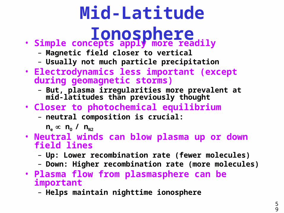
Mid-Latitude Ionosphere• Simple concepts apply more readily
– Magnetic field closer to vertical– Usually not much particle precipitation
• Electrodynamics less important (except during geomagnetic storms)– But, plasma irregularities more prevalent at mid-
latitudes than previously thought• Closer to photochemical equilibrium
– neutral composition is crucial:ne nO / nN2
• Neutral winds can blow plasma up or down field lines– Up: Lower recombination rate (fewer molecules)– Down: Higher recombination rate (more molecules)
• Plasma flow from plasmasphere can be important– Helps maintain nighttime ionosphere
60
Mid-Latitude Ionosphere, cont.
• Various diurnal and seasonal “anomalies”– See Tascione, 8.4
• Strong solar cycle variation associated with Solar EUV Radiation

61
High Latitude Ionosphere
• Magnetic field lines – “Open” over polar region– Closed in auroral oval, but extend deep
into magnetotail
• Main coupling region to magnetosphere– But, during geomagnetic storms, E
fields can penetrate to lower latitudes
62
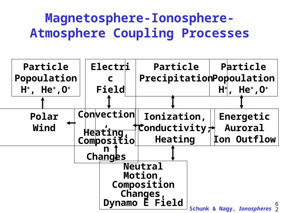
Magnetosphere-Ionosphere-Atmosphere Coupling Processes
ParticlePopoulation
H+, He+,O+
ElectricField
ParticlePrecipitation
PolarWind
ParticlePopoulation
H+, He+,O+
Convection,Heating,
CompositionChanges
Ionization,Conductivity,
Heating
EnergeticAuroral
Ion Outflow
Neutral Motion,Composition
Changes,Dynamo E Field
Schunk & Nagy, Ionospheres
63
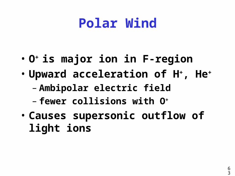
Polar Wind
• O+ is major ion in F-region
• Upward acceleration of H+, He+
– Ambipolar electric field – fewer collisions with O+
• Causes supersonic outflow of light ions

64
Electric Field
Schunk & Nagy, Ionospheres

65
Electric Field, cont.
• Solar wind motion (Vsw) contains electric field: E = - Vsw x B
• Near-Earth sees electric field that points in dawn to dusk direction
• E-field maps down highly conducting field lines into ionosphere
• This “convection” E causes E x B drift of ionospheric plasma in anti-sun direction
• Farther from Earth, E x B drift is toward the equatorial plane

66
Electric Field, cont.
• Charges on polar cap boundary induce E fields on nearby closed field lines, opposite to convection electric field
• Ionospheric plasma on closed field lines drifts sunward in response
• On boundary of open and closed field lines, field-aligned currents flow between the magnetosphere and ionosphere
67
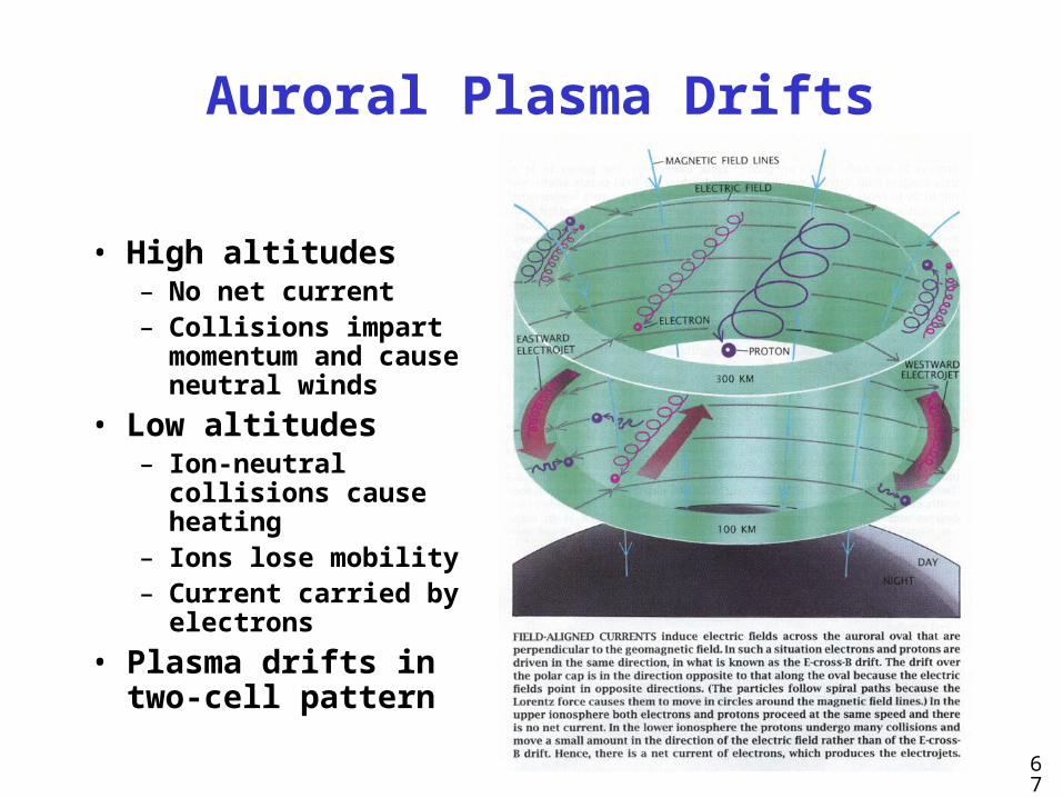
Auroral Plasma Drifts
• High altitudes– No net current– Collisions impart
momentum and cause neutral winds
• Low altitudes– Ion-neutral
collisions cause heating
– Ions lose mobility– Current carried by
electrons
• Plasma drifts in two-cell pattern
68
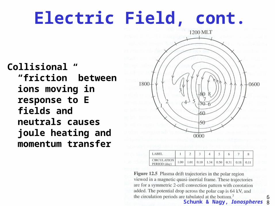
Electric Field, cont.
Collisional “friction” between ions moving in response to E fields and neutrals causes joule heating and momentum transfer
Schunk & Nagy, Ionospheres
69
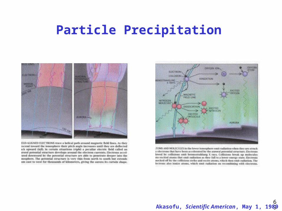
Particle Precipitation
Akasofu, Scientific American, May 1, 1989
70
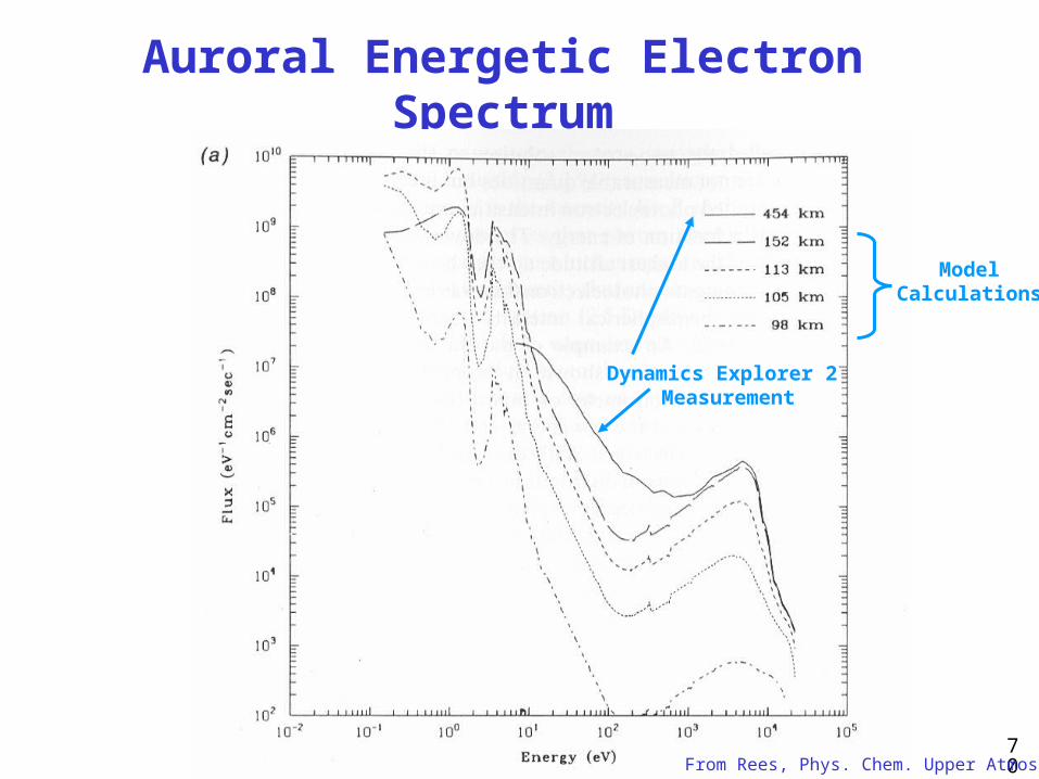
Auroral Energetic Electron Spectrum
Dynamics Explorer 2 Measurement
ModelCalculations
From Rees, Phys. Chem. Upper Atmos.

71
Ionization Rates by Energetic Auroral Electrons
From Rees, Phys. Chem. Upper Atmos.
72
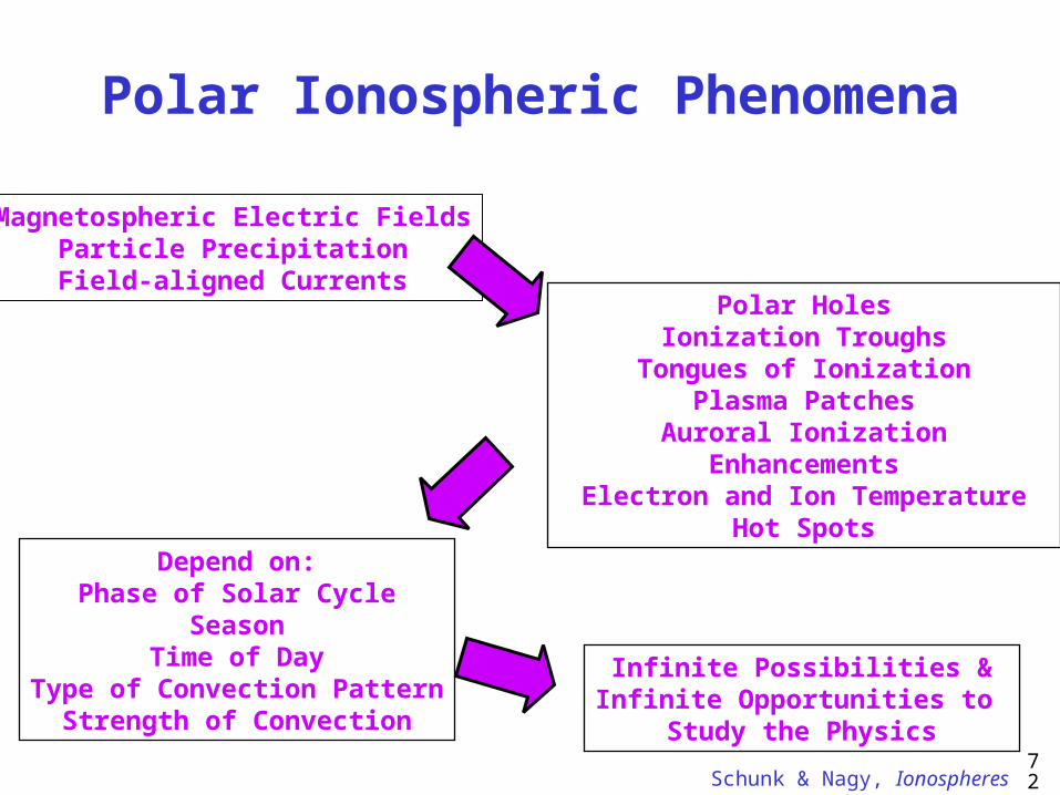
Polar Ionospheric Phenomena
Magnetospheric Electric FieldsParticle Precipitation
Field-aligned CurrentsPolar Holes
Ionization TroughsTongues of Ionization
Plasma PatchesAuroral Ionization EnhancementsElectron and Ion Temperature Hot
Spots
Depend on:Phase of Solar Cycle
SeasonTime of Day
Type of Convection PatternStrength of Convection
Infinite Possibilities &Infinite Opportunities to
Study the Physics
Schunk & Nagy, Ionospheres
73
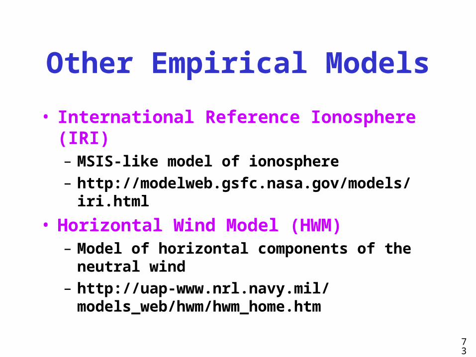
Other Empirical Models
• International Reference Ionosphere (IRI)– MSIS-like model of ionosphere– http://modelweb.gsfc.nasa.gov/models/iri.html
• Horizontal Wind Model (HWM)– Model of horizontal components of the neutral
wind– http://uap-www.nrl.navy.mil/models_web/
hwm/hwm_home.htm