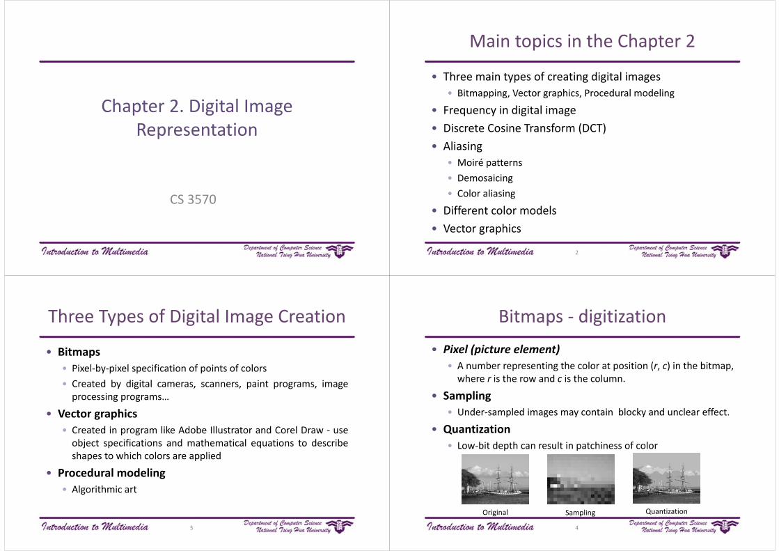
Chapter 2. Digital Image Representation

CS 3570

Main topics in the Chapter 2

• Three main types of creating digital images• Bitmapping, Vector graphics, Procedural modeling

• Frequency in digital image • Discrete Cosine Transform (DCT)• Aliasing

• Moiré patterns• Demosaicing• Color aliasing

• Different color models• Vector graphics

2

Three Types of Digital Image Creation

• Bitmaps• Pixel‐by‐pixel specification of points of colors• Created by digital cameras, scanners, paint programs, imageprocessing programs…

• Vector graphics• Created in program like Adobe Illustrator and Corel Draw ‐ useobject specifications and mathematical equations to describeshapes to which colors are applied

• Procedural modeling• Algorithmic art

3

Bitmaps ‐ digitization• Pixel (picture element)

• A number representing the color at position (r, c) in the bitmap, where r is the row and c is the column.

• Sampling• Under‐sampled images may contain  blocky and unclear effect.

• Quantization• Low‐bit depth can result in patchiness of color

4

Original Sampling Quantization

Bitmaps – pixel dimensions & resolution

• Pixel dimensions• The number of pixels horizontally (i.e., width, w) and vertically(i.e., height, h), denoted w × h

• Resolution• The number of pixels in an image file per unit of spatialmeasure

• Resolution can be measured in pixels per inch, abbreviated ppi.A 200 ppi image will print out using 200 pixels to determine thecolors for each inch

• Resolution of a printer is a matter of how many dots of color itcan print over an area. A common measurement is dots perinch (DPI).

5

Bitmaps – image size• Image size

• The physical dimensions of an image when it is printed out or displayed on a computer

• Relation of image size, pixel dimension and resolution• a = w/r , b = h/r• Resolution r,  Pixel dimensions w x h, Printed image size a x b

• Different image size

6

Frequency in digital image 

• An image as a function that can be represented in a graph• y = f(x)• x: the position of one point• y: the color value at position x• f: a function over the spatial domain when the x values correspond to points in space

• In the realm of digital imaging, frequency refers to the rate at which color values change.

7

Frequency in digital image• An image in which colorvaries continuously fromlight gray to dark grayand back again

• Discretized version ofgradient

8

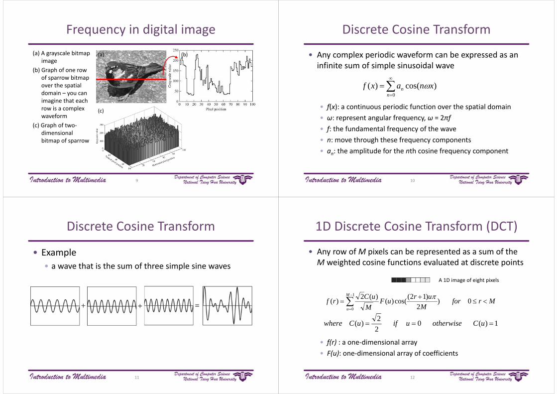
Frequency in digital image(a) A grayscale bitmap 

image(b) Graph of one row 

of sparrow bitmap over the spatial domain – you can imagine that each row is a complex waveform

(c) Graph of two‐dimensional bitmap of sparrow

(a) (b)

(c)

9

Discrete Cosine Transform

• Any complex periodic waveform can be expressed as an infinite sum of simple sinusoidal wave

• f(x): a continuous periodic function over the spatial domain• ω: represent angular frequency, ω = 2πf• f: the fundamental frequency of the wave• n: move through these frequency components• an: the amplitude for the nth cosine frequency component

0

)cos()(n

n xnaxf

10

Discrete Cosine Transform

• Example• a wave that is the sum of three simple sine waves

11

1D Discrete Cosine Transform (DCT)

• Any row of M pixels can be represented as a sum of the M weighted cosine functions evaluated at discrete points

• f(r) : a one‐dimensional array• F(u): one‐dimensional array of coefficients

MrforM

uruFM

uCrfM

u

0)2

)12(cos()()(2)(1

0

1)(022)( uCotherwiseuifuCwhere

12

A 1D image of eight pixels

1D DCT

• Basis function:                       , M=8 )2

)12(cos(M

ur

)16

0)12(cos( r

)16

)12(cos( r

)16

2)12(cos( r

)16

3)12(cos( r

)16

4)12(cos( r

)16

5)12(cos( r

)16

6)12(cos( r

)16

7)12(cos( r

13

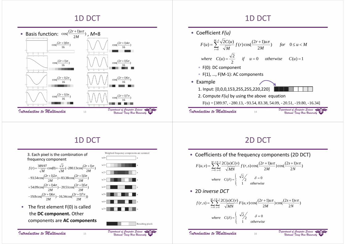
1D DCT• Coefficient F(u)

• F(0): DC component• F(1), …, F(M‐1): AC components

• Example1. Input: [0,0,0,153,255,255,220,220]2. Compute F(u) by using the above  equation

MuforM

urrfM

uCuFM

r

0)2

)12(cos()()(2)(1

0

1)(022)( uCotherwiseuifuCwhere

14

16.34]- 19.80,- 20.51,- 54.09, 83.38, 93.54,- 280.13,- [389.97,=F(u)

1D DCT3. Each pixel is the combination of frequency component

• The first element F(0) is called the DC component. Other components are AC components

))2

7)12(cos(34.16)2

6)12(cos(8.19

)2

5)12(cos(51.20)2

4)12(cos(09.54

)2

3)12(cos(38.83)2

2)12(cos(54.93

)2

)12(cos(13.280(2)0cos(97.389)(

Mr

Mr

Mr

Mr

Mr

Mr

Mr

MMrf

15

2D DCT• Coefficients of the frequency components (2D DCT)

• 2D inverse DCT

1

0

1

0)

2)12(cos()

2)12(cos(),()()(2),(

M

r

N

s Nvs

Mursrf

MNvCuCvuF

1

0

1

0)

2)12(cos()

2)12(cos(),()()(2),(

M

r

N

s Nvs

MurvuF

MNvCuCsrf

otherwiseCwhere

102

2)(

otherwiseCwhere

102

2)(

16

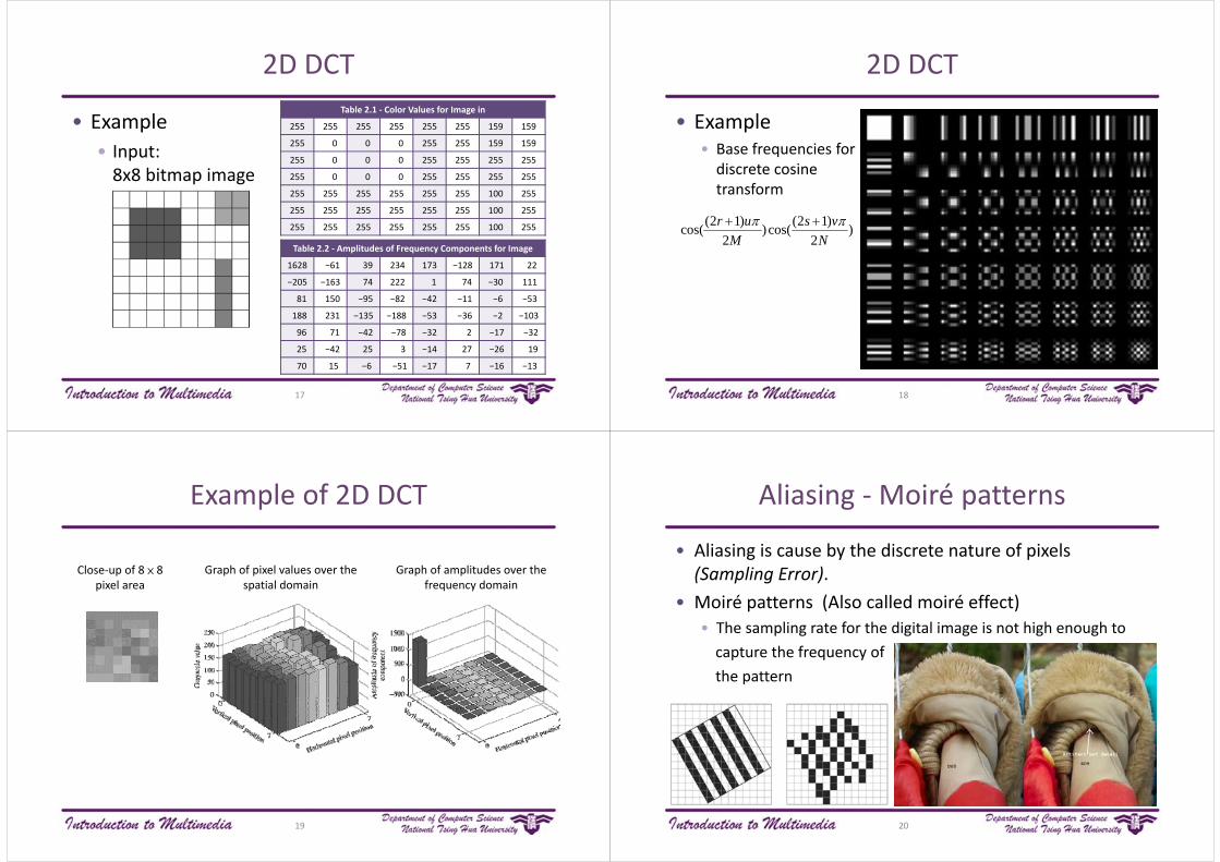
2D DCT

• Example• Input: 8x8 bitmap image

Table 2.1 ‐ Color Values for Image in

255 255 255 255 255 255 159 159

255 0 0 0 255 255 159 159

255 0 0 0 255 255 255 255

255 0 0 0 255 255 255 255

255 255 255 255 255 255 100 255

255 255 255 255 255 255 100 255

255 255 255 255 255 255 100 255

Table 2.2 ‐ Amplitudes of Frequency Components for Image

1628 −61 39 234 173 −128 171 22

−205 −163 74 222 1 74 −30 111

81 150 −95 −82 −42 −11 −6 −53

188 231 −135 −188 −53 −36 −2 −103

96 71 −42 −78 −32 2 −17 −32

25 −42 25 3 −14 27 −26 19

70 15 −6 −51 −17 7 −16 −13

17

2D DCT

• Example• Base frequencies for discrete cosine transform

)2

)12(cos()2

)12(cos(N

vsM

ur

18

Example of 2D DCT

Close‐up of 8 × 8 pixel area

Graph of pixel values over the spatial domain

Graph of amplitudes over the frequency domain

19

Aliasing ‐Moiré patterns 

• Aliasing is cause by the discrete nature of pixels (Sampling Error).

• Moiré patterns  (Also called moiré effect)• The sampling rate for the digital image is not high enough to capture the frequency of the pattern

20

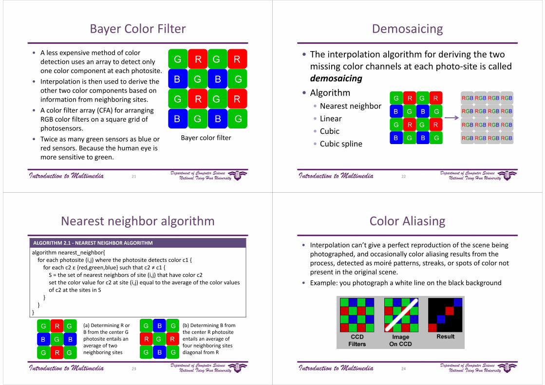
Bayer Color Filter

• A less expensive method of color detection uses an array to detect only one color component at each photosite. 

• Interpolation is then used to derive the other two color components based on information from neighboring sites. 

• A color filter array (CFA) for arranging RGB color filters on a square grid of photosensors.

• Twice as many green sensors as blue or red sensors. Because the human eye is more sensitive to green.

Bayer color filter

21

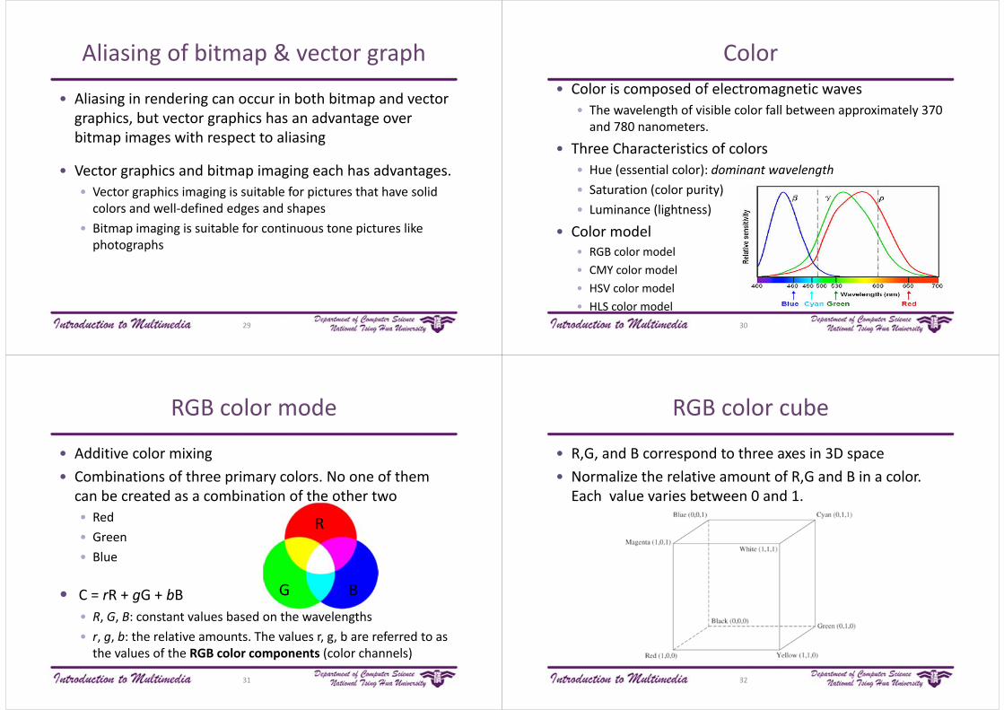
Demosaicing

• The interpolation algorithm for deriving the two missing color channels at each photo‐site is called demosaicing

• Algorithm• Nearest neighbor• Linear• Cubic• Cubic spline

22

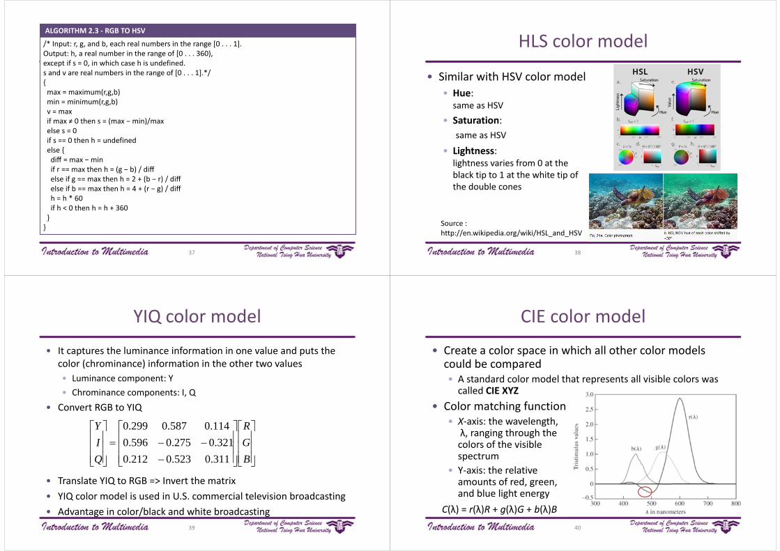
Nearest neighbor algorithmALGORITHM 2.1 ‐ NEAREST NEIGHBOR ALGORITHM

algorithm nearest_neighbor{for each photosite (i,j) where the photosite detects color c1 { for each c2 ε {red,green,blue} such that c2 ≠ c1 { S = the set of nearest neighbors of site (i,j) that have color c2 set the color value for c2 at site (i,j) equal to the average of the color values of c2 at the sites in S 

}} 

} 

(a) Determining R or B from the center G photosite entails an average of two neighboring sites

(b) Determining B from the center R photositeentails an average of four neighboring sites diagonal from R

23

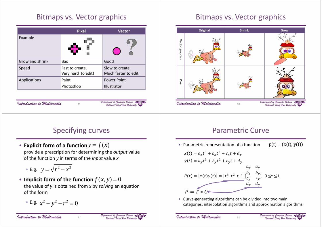
Color Aliasing

• Interpolation can’t give a perfect reproduction of the scene being photographed, and occasionally color aliasing results from the process, detected as moiré patterns, streaks, or spots of color not present in the original scene.

• Example: you photograph a white line on the black background

24

Aliasing ‐ Jagged Edges

• Aliasing used to describe the jagged edges along lines or edges that are drawn at an angle across a computer screen

• A line on a computer screen is made up of discrete units: pixels

Aliasing of a line that is one pixel wide

25

Algorithm 2.2 for drawing a line

• Left figure shows a line that is two pixels wide going from point (8, 1) to point (2, 15)

• In right figure a pixel is colored black if at least half its area is covered by the two‐pixel line

Drawing a line two pixels wide Line two pixels wide, aliased

26

Anti‐aliasing

• Anti‐aliasing is a technique for reducing the jaggedness of lines or edges caused by aliasing

• The idea is to color a pixel with a shade of its designated color in proportion to the amount of the pixel that is covered by the line or edge

a line two pixels wide Line two pixels wide, anti‐aliased

27

Aliasing of bitmap & vector graph

• Vector graphics suffer less from aliasing problems than do bitmap images in that vector graphics images can be resized without loss of resolution

• Upsampling• The image is later enlarged by increasing the number of pixels

Bitmap Vector Graph

28

Aliasing of bitmap & vector graph

• Aliasing in rendering can occur in both bitmap and vector graphics, but vector graphics has an advantage over bitmap images with respect to aliasing

• Vector graphics and bitmap imaging each has advantages. • Vector graphics imaging is suitable for pictures that have solid colors and well‐defined edges and shapes

• Bitmap imaging is suitable for continuous tone pictures like photographs

29

Color• Color is composed of electromagnetic waves

• The wavelength of visible color fall between approximately 370 and 780 nanometers.

• Three Characteristics of colors• Hue (essential color): dominant wavelength• Saturation (color purity)• Luminance (lightness)

• Color model• RGB color model• CMY color model• HSV color model• HLS color model

30

RGB color mode

• Additive color mixing• Combinations of three primary colors. No one of them can be created as a combination of the other two• Red• Green• Blue

• C = rR + gG + bB• R, G, B: constant values based on the wavelengths• r, g, b: the relative amounts. The values r, g, b are referred to as the values of the RGB color components (color channels) 

R

G B

31

RGB color cube

• R,G, and B correspond to three axes in 3D space• Normalize the relative amount of R,G and B in a color. Each  value varies between 0 and 1.

32

RGB color to grayscale

• The conversion of RGB color to grayscale• In RGB color (R, G, B)• In grayscale (L, L, L)

• Since all three color components are equal in a gray pixel, only one of the three values needs to be stored. Thus a 24‐bit RGB pixel can be stored as an 8‐bit grayscale pixel.

L = 0.30R + 0.59G + 0.11B

33

RGB color model –advantage & disadvantage

• Advantage• The human eye perceives color• The computer monitor can be engineered to display color

• Disadvantage• Exist visible colors that can’t be represented with positive value for each of the red, green and blur components

• It is necessary to “subtract out” some of the red, green, or blue in the combined beams to match the pure color

34

CMY color model• Subtractive color mixing• Commonly used in printing• It has three primaries

• Cyan, Magenta, Yellow

• Conversion between RGB and CMY color models• C = 1 – R, M = 1‐G,  Y = 1 – B

• CMYK model• In CMY color mode, the maximum amount of three primary should combine to black, but in fact producing a dark brown

• Add a pure black ‐> K• K = min(C, M, Y),  Cnew = C – K,  Mnew = M – K,  Ynew = Y ‐ K

Cyan

Magenta Yellow

35

HSV color model

• Represent color by three terms• Hue, the color type (such as red, blue, or yellow)Ranges from 0‐360 (but normalized to 0‐100% in some applications) 

• Saturation, the "vibrancy" of the colorRanges from 0‐100%The lower the saturation of a color, 

the more “grayness”• Value, the brightness of the colorRanges from 0‐100%

• Also called HSB(hue, saturation and brightness)

36

RGB to HSVALGORITHM 2.3 ‐ RGB TO HSV

/* Input: r, g, and b, each real numbers in the range [0 . . . 1].Output: h, a real number in the range of [0 . . . 360), except if s = 0, in which case h is undefined. s and v are real numbers in the range of [0 . . . 1].*/{max = maximum(r,g,b)min = minimum(r,g,b)v = maxif max ≠ 0 then s = (max − min)/maxelse s = 0if s == 0 then h = undefinedelse {diff = max − minif r == max then h = (g − b) / diffelse if g == max then h = 2 + (b − r) / diffelse if b == max then h = 4 + (r − g) / diffh = h * 60if h < 0 then h = h + 360}}

37

HLS color model

• Similar with HSV color model• Hue:

same as HSV• Saturation:

same as HSV

• Lightness:lightness varies from 0 at the black tip to 1 at the white tip of the double cones

38

Source : http://en.wikipedia.org/wiki/HSL_and_HSV

YIQ color model

• It captures the luminance information in one value and puts the color (chrominance) information in the other two values• Luminance component: Y• Chrominance components: I, Q

• Convert RGB to YIQ

• Translate YIQ to RGB => Invert the matrix• YIQ color model is used in U.S. commercial television broadcasting• Advantage in color/black and white broadcasting

BGR

QIY

311.0523.0212.0321.0275.0596.0

114.0587.0299.0

39

CIE color model

• Create a color space in which all other color models could be compared• A standard color model that represents all visible colors was called CIE XYZ

• Color matching function• X‐axis: the wavelength,

λ, ranging through thecolors of the visible spectrum

• Y‐axis: the relative amounts of red, green, and blue light energy

C(λ) = r(λ)R + g(λ)G + b(λ)B40

CIE color model

• CIE XYZ• No three visible primary colors that can be combined in positive amounts to create all colors

• Use three “virtual ” primaries—called X, Y, and Z—are purely theoretical rather than physical entities.

• Linear transform of the previous space

C(λ) = x(λ)X + y(λ)Y + z(λ)Z

41

CIE color model

• Can think of X, Y , Z as coordinates• Linear transform from typical RGB or LMS0.41 0.36 0.180.21 0.72 0.070.02 0.12 0.953.24 1.54 0.50.97 1.88 0.040.06 0.2 1.06

42

Chromaticity and CIE color space

• Chromaticity values

• Visible color spectrum projected onto the X + Y + Z = 1 plane

43

CIE color model

• RGB color space• CMYK color space• The gamut for RGB color is larger than the CMYK gamut. However, neither color space is entirely contained within the other.

44

CIE L*a* b*, CIE L*U*V*, and Perceptual Uniformity

• The CIE XYZ model has three main advantages: • device‐independent• provides a way to represent all visible colors• representation is based upon spectrophotometricmeasurements of color.

• A remaining disadvantage of the CIE XYZ model is that it is not perceptually uniform.

• In a perceptually uniform color space, the distance between two points is directly proportional to the perceived difference between the two colors.

45

CIE L*a* b*, CIE L*U*V*

• CIE L*a*b* is a subtractive color model in which the L* axis gives brightness values varying from 0 to 100, the a axis moves from red (positive values) to green (negative values), and the b axis moves from yellow (positive values) to blue (negative values). 

• CIE L*U*V is an additive color model that was similarly constructed to achieve perceptual uniformity, but that was less convenient in practical usage.

• Because the CIE L*a*b* model can represent all visible colors, it is generally used as the intermediate color model in conversions between other color models.

46

Image in different color models

• Source : http://en.wikipedia.org/wiki/HSL_and_HSV

47

Vector Graphics

• Vector graphics is an image file format suitable for pictures with areas of solid, clearly separated colors—cartoon images, logos, and the like.

• Instead of being painted pixel by pixel, a vector graphic image is drawn object by object in terms of each object’s geometric shape.

• Many file formats for vector graphics—.fh, .ai, .wmf, .eps, etc.—they contain the parameters to mathematical formulas defining how shapes are drawn.• A line can be specified by its endpoints, a square by the length of a side, a rectangle by the length of two sides, a circle by radius

48

Bitmaps vs. Vector graphics

Pixel VectorExample

Grow and shrink Bad GoodSpeed Fast to create.  

Very hard  to edit!Slow to create.   Much faster to edit.

Applications PaintPhotoshop

Power PointIllustrator

49

Bitmaps vs. Vector graphicsOriginal Shrink Grow

Vector graphicsPixel

50

Specifying curves

• Explicit form of a functionprovide a prescription for determining the output value of the function y in terms of the input value x

• E.g.

• Implicit form of the functionthe value of y is obtained from x by solving an equation of the form

• E.g.

)(xfy

0),( yxf

22 xry

0222 ryx

51

Parametric Curve

• Parametric representation of a function

• Curve‐generating algorithms can be divided into two main categories: interpolation algorithms and approximation algorithms.

y(t))(x(t),p(t)

1 0 t 1

52

Bézier curves

• A Bézier curve is a parametric curve described by polynomials based on any number of control points• Degree of polynomials = number of points – 1• A Bézier curve passes through its first and last control points, but, in general, no others.

53

Bézier curve

• A Bézier curve is defined by a cubic polynomial equation• P(t) = T *M * G• T = [t3 t2 t 1], M is called the basis matrix. G is called 

the geometry matrix.

• The blending functions are given by T *M,P(t) = (T *M) * G = (1 − t)3p0 + 3t(1 − t)2p1 + 3t2(1 − t)p2 + t3p3

54

Blending Function

• Bézier curves can be described in terms of the blending functions

• In the blending functions blendingk,n(t), n is the degree of the polynomial and k refers to the “weight” for the kth term in the polynomial.

blendingk,n(t) = C(n, k)tk (1 − t)n−k

• For cubic polynomials, blending0,3=(1 − t)3,  blending1,3=3t(1 − t)2

blending2,3=3t2(1 − t),  blending3,3=t3

55

de Casteljau algorithm• For constructing a Bézier curve recursively• Two endpoints p0,p3 and two interior control points p1, p2.

56

Bézier curves –advantage & disadvantages

• Advantage• Very simple

• Disadvantages• Expensive to evaluate the curve at many points• No easy way of knowing how fine to sample points, and maybe sampling rate must be different along curve

• No easy way to adapt. In particular, it is hard to measure the deviation of a line segment from the exact curve

57

Examples of Bézier curves

58

Procedural modeling

• You create a digital image by writing a computer program based on some mathematicalcomputation or unique type of algorithm• Procedural models are often defined by a small set of data that describes the overall properties of the model. For example, a tree might be defined by some branching properties and leaf shapes

• The actual model is constructed by a procedure that often makes use of randomness to add variety. In this way, a single tree pattern can be used to model an entire forest

59

Procedural modeling – fractal

• fractal ‐ algorithmic art • Fractal : a graphical image characterized by a recursively repeating structure

• Fractals exist in natural phenomena.• If you look at the image at the macro‐level—the entire structure—you’ll see a certain geometric pattern, and then when you zoom in on a smaller scale, you’ll see that same pattern again

Natural fractal structure

60

Procedural modeling – fractal

• fractal is created with a recursive program that draws the same shape down to some base level.

• Koch’s snowflake, a recursively defined fractal

• Sierpinski’s gasket

61

Procedural modeling –mandelbrot fractal

• A beautiful and complex geometry emerges from the nature of the computation 

• The Mandelbrot fractal computation is based on a simple iterative equation• 2• z and c are complex numbers. c=cr+cii, z=zr+zii• The output of the ith computation is the input z to the i + 1st computation

62

Procedural modeling –mandelbrot fractal

Goal: determine the color of each pixel1) Initial

• Complex number c <‐> pixel position • Complex number z = 0

2) f(z)=z2+c  iterativelyThe output of the ith computation is the input z to the i + 1st computation

3) The color of pixel• Black: the computation has not revealed 

itself as being unbounded• Color: related to how many iterations were 

performed

63

Procedural modeling –mandelbrot fractal ‐ 3

ALGORITHM 2.5 – Mandelbrot Fractal 

/*Input: Horizontal and vertical ranges of the complex number plane.Output: A bitmap for a fractal.*/{/*constant MAX is the maximum number of iterations*/for each pixel in the bitmap {map pixel coordinates (x,y) to complex number plane coordinates (cr, ci)num_iterations = 0z = 0while num_iterations < MAX and not_unbounded* {z = z2 + cnum_iterations = num_iterations + 1}

/*map_color(x,y) uses the programmer’s chosen color map to determine the color ofeach pixel based on how many iterations are done before the computation is found tobe unbounded*/if num_iterations == MAX then color(x,y) = BLACKelse color(x,y) = map_color(num_iterations)}}

64

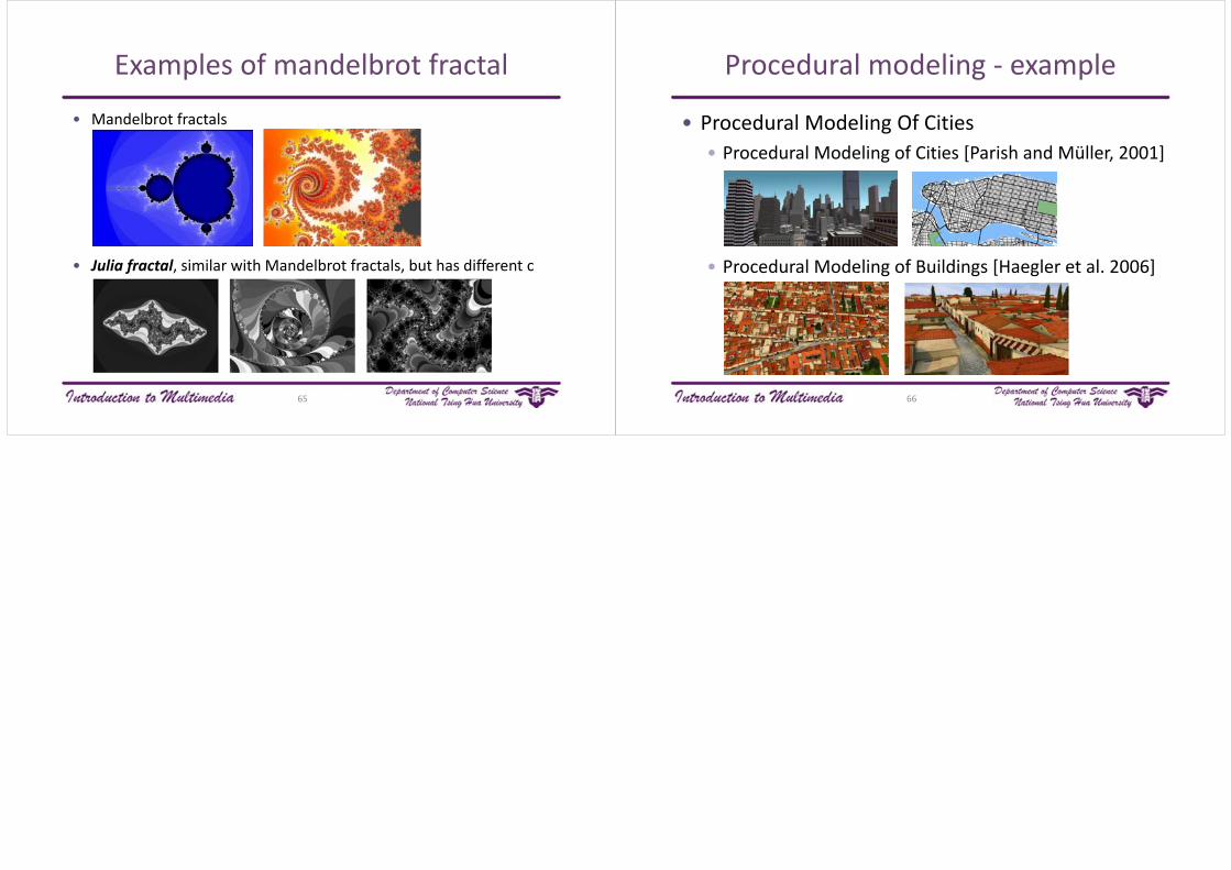
Examples of mandelbrot fractal

• Mandelbrot fractals

• Julia fractal, similar with Mandelbrot fractals, but has different c

65

Procedural modeling ‐ example

• Procedural Modeling Of Cities• Procedural Modeling of Cities [Parish and Müller, 2001]

• Procedural Modeling of Buildings [Haegler et al. 2006]

66