Embed Size (px)
Citation preview

Topological Parameters forTime-Space Tradeoff
Rina DechterInformation & Computer Science
University of CaliforniaIrvine, CA 92717
Yousri El FattahRockwell Science Center1049 Camino Dos Rios
Thousand Oaks, CA 91360
March 17, 2000
Abstract
In this paper we propose a family of algorithms combining tree-clustering with conditioning that trade space for time. Such algo-rithms are useful for reasoning in probabilistic and deterministic net-works as well as for accomplishing optimization tasks. By analyzingthe problem structure the user can select from a spectrum of algo-rithms, the one that best meets a given time-space specification. Todetermine the potential of this approach, we analyze the structuralproperties of problems coming from the circuit diagnosis domain. Theanalysis demonstrate how the tradeoffs associated with various hybridscan be explicated and be used for each problem instance.
1 Introduction
Problem solving methods can be viewed as hybrids of two main principles:inference and search. Tree-clustering is an example to an inference algorithmwhile the cycle-cutset is an example of a search method. Tree clustering algo-rithms are time and space exponential in the size of their cliques while searchalgorithms are time exponential but require only linear memory. In this paperwe developed a hybrid scheme that uses inference (tree-clustering) and search
1

(cycle-cutset conditioning) as its two extremes and, using a single, structure-based design parameter, permits the user to control the storage-time tradeoffin accordance with its problem domain and the available resources.
Topology-based algorithms for constraint satisfaction and probabilisticreasoning fall into two distinct classes. One class is centered on tree-clustering,the other on cycle-cutset decomposition. Tree-clustering involves transform-ing the original problem into a tree-like problem [26, 22, 14] that can thenbe solved by a specialized efficient tree-solving algorithm [27, 28]. The trans-forming algorithm identifies subproblems that together form a tree, and thesolutions to the subproblems serve as the new values of variables in a treemetalevel problem. The metalevel problem is called a join-tree. The tree-clustering algorithm is time and space exponential in the tree-width of theproblem’s graph. A related parameter is the induced-width which equals thetree-width. We will use both terms interchangeably.
The cycle-cutset method, also called loop-cutset conditioning, utilizes theproblem’s structure in a different way. It exploit the fact that variable in-stantiation changes the effective connectivity of the underlying graph. Acycle-cutset of an undirected graph is a subset of its nodes which, once re-moved, cuts all of the graph’s cycles. A typical cycle-cutset method enu-merates the possible assignments to a set of cutset variables and, for eachcutset assignment, solves (or reasons about) a tree-like problem in polyno-mial time. Thus, the overall time complexity is exponential in the size ofthe cycle-cutset [8, 29, 15]. Fortunately, enumerating all the cutset’s assign-ments can be accomplished in linear space, yielding an overall linear spacealgorithm.
The first question is which method, tree-clustering or the cycle-cutsetscheme provide a better worst-case time guarantees. This question was an-swered by Bertele and Briochi [5] in 1972 and later reaffirmed in [31]. Theyshowed that, the minimal cycle-cutset of any graph can be much larger, andis never smaller than its minimal tree-width. In fact, for an arbitrary graph,r ≤ c + 1, where c is the minimal cycle-cutset and r is the tree-width [5].Consequently, for any problem instance the time guarantees accompanyingthe cycle-cutset scheme are never tighter than those of tree-clustering, andcan be even much worse. On the other hand, while tree-clustering requiresexponential space (in the induced-width) the cycle-cutset requires only linearspace.
Since the space complexity of tree-clustering can severely limit its useful-
2

ness, we investigate in this paper the extent to which space complexity canbe reduced, while reasonable time complexity guarantees are maintained. Isit possible to have the time guarantees of clustering while using linear space?On some problem instances, it is possible. Specifically, on those problemswhose associated graph has an induced width and a cycle-cutset of compara-ble sizes (e.g., on a ring, the cutset size is 1 and the tree width is 2, leadingto identical time bounds). We conjecture, however, that any algorithm thathas a time bound guarantee exponential in the induced-width will, on someproblem instances, require exponential space in the induced width.
The space complexity of tree-clustering can be bounded more tightly usingthe separator size, which is defined as the size of the maximum subset ofvariables shared by adjacent subproblems in the join-tree. Indeed some ofthe variants of tree-clustering algorithms send messages over the separatorsonly and therefore can comply with space complexity that is exponential inthe separator size only [22, 38]. Our investigation employs the separatorsize to control the time-space tradeoff. The idea is to combine adjacentsubproblems joined by a large separator into one bigger cluster or subproblemso that the remaining separators are of smaller size. Once a join-tree withsmaller separators is generated, its potentially larger clusters can be solvedusing the cycle-cutset method, or any other linear-space scheme.
In this paper we will develop a time-space tradeoff scheme that is appli-cable to belief network processing, constraint processing, and optimizationtasks, yielding a sequence of parameterized algorithms that can trade spacefor time. With this scheme it will be possible to select from a spectrumof algorithms the one that best meets some time-space requirement. Algo-rithm tree-clustering and cycle-cutset conditioning are two extremes in thisspectrum.
We investigate the potential of our scheme in the domain of combinato-rial circuits. This domain is frequently used as an application area in bothprobabilistic and deterministic reasoning [18, 40, 16]. We analyze 11 bench-mark combinatorial circuits widely used in the fault diagnosis and testingcommunity [6] (see Table 1 ahead.). For each circuit, the analysis is summa-rized in a chart displaying the time-space complexity tradeoffs for diagnosingthat circuit. The analysis allows tailoring the hybrid of tree-clustering andcycle-cutset decomposition to the available memory.
Different variants of the tree-clustering transformation algorithms weredeveloped in recent years, both for constraint processing ([11]) and for prob-
3
abilistic inference [29, 26, 22, 37, 38, 24, 23]. Some of these algorithms compilefunctions over the cliques and some restrict this information to the separa-tors. Some are directional, query-based while others are symmetrical, com-piling answers for a variety of queries. We choose to demonstrate our ideausing a directional variant of tree-clustering that is query-based, which wehope simplify the exposition. The approach is applicable to any variant oftree-clustering.
Section 2 gives definitions and preliminaries and introduces the time-space tradeoff ideas for belief networks. Sections 3 and 4 briefly extend theseideas to constraint networks and to optimization problems. Section 5 and 6describe the empirical analysis and the results. Section 7 discusses relatedwork and Section 8 gives our conclusions.
The paper assumes familiarity with the basic concepts of tree-clusteringand cycle-cutset conditioning and provides only brief necessary background.For more details the reader should consult the references.
2 Probabilistic Networks
2.1 Overview
2.1.1 Definitions and notations
Belief networks provide a formalism for reasoning about partial beliefs underconditions of uncertainty. It is defined by a directed acyclic graph over nodesrepresenting random variables of interest (e.g., the temperature of a device,the gender of a patient, a feature of an object, the occurrence of an event).The arcs signify the existence of direct causal influences between the linkedvariables. The strength of these influences are quantified by conditionalprobabilities that are attached to each cluster of parents-child nodes in thenetwork. A belief network is a concise description of a complete probabilitydistribution. It uses the concept of a directed graph.
Definition 1 [Directed graph] A directed graph G = {V, E}, where V ={X1, ..., Xn} is a set of elements and E = {(Xi, Xj)|Xi, Xj ∈ V } is the setof edges. If an arc (Xi, Xj) ∈ E, we say that Xi points to Xj . For eachvariable Xi, pa(Xi) is the set of variables pointing to Xi in G, while ch(Xi)is the set of variables that Xi points to. The family of Xi includes Xi and its
4

parent variables. A directed graph is acyclic if it has no directed cycles. In anundirected graph the direction of the arcs is ignored: (Xi, Xj) and (Xj, Xi)are identical. An undirected graph is chordal if every cycle of length at least4 has a chord. A clique is a subgraph that is completely connected and amaximal clique of graph is a clique that is not contained in any other cliqueof the graph.
Definition 2 [Belief Networks] Let X = {X1, ..., Xn} be a set of random vari-ables over multi-valued domains, D1, ..., Dn. A belief network is a pair (G, P )where G is a directed acyclic graph over the nodes X and P = {Pi} are theconditional probability matrices over the families of G, Pi = P (Xi|pa(Xi)).An assignment (X1 = x1, ..., Xn = xn) can be abbreviated as x = (x1, ..., xn).The belief network represents a probability distribution over X having theproduct form
P (x1, ...., xn) = Πni=1P (xi|xpa(Xi))
where xpa(Xi) denotes the projection of a tuple x over pa(Xi). An evidenceset e is an instantiated subset of variables. A moral graph of a belief networkis an undirected graph generated by connecting the tails of any two head-to-head pointing arcs in G and removing the arrows. A belief network isa polytree if its underlying undirected (unmoralized) graph has no cycles(namely, it is a tree).
Definition 3 [Induced width, induced graph] An ordered graph is a pair(G, d) where G is an undirected graph and d = X1, ..., Xn is an ordering ofthe nodes. The width of a node in an ordered graph is the number of itsearlier neighbors. The width w(d) of an ordering d, is the maximum widthover all nodes. The induced width of an ordered graph, w∗(d), is the width ofthe induced ordered graph obtained by processing the nodes recursively, fromlast to first; when node X is processed, all its earlier neighbors are connected.This process is also called “triangulation”. The induced (triangulated) graphis clearly chordal. The induced width of a graph, w∗, is the minimal inducedwidth over all its orderings (For more information see [13, 9].
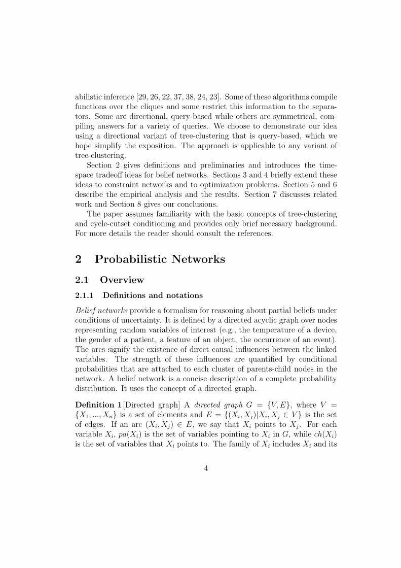
Example 1: Figure 1 shows a belief network’s acyclic graph and its asso-ciated moral graph. The width of the graph in Figure 1b along the orderingd = A, B, C, D, G, E, F, H is 3. Since the moral graph in Figure 1(b) ischordal no arc is added when generating the induced ordered graph. There-fore, the induced-width w∗ of the graph is also 3.
5

A
B
CD E
FG
H A
B
CD E
FG
H
Figure 1: (a) A belief network and (b) its moral graph
The most common task over belief networks is to determine posteriorbeliefs of some variables. Other important tasks are mpe: finding the mostprobable explanation given a set of observations, or map: finding the max-imum aposteriori hypotheses given evidence, both tasks are relevant to ab-duction and diagnosis [29]. It is well known that such tasks can be answeredeffectively for singly-connected polytrees by a belief propagation algorithm[29] that can be extended to multiply-connected networks by either tree-clustering or loop-cutset conditioning.
2.1.2 Tree-Clustering
The most widely used method for processing belief networks is join-tree clus-tering. The algorithm transforms the original network into a tree of subprob-lems called join-tree. Tree-clustering methods have two parts. In the firstpart the structure of the newly generated tree problem is decided, and in thesecond part the conditional probabilities between the subproblems, (viewedas high-dimensional variables) is determined. The structure of the join-treeis determined primarily by graph information, embedding the graph in a treeof cliques as follows. First the moral graph is embedded in a chordal graphby adding some edges. This is accomplished by picking a variable orderingd = X1, ..., Xn, then, moving from Xn to X1, recursively, connecting all theearlier neighbors of Xi in the moral graph yielding the induced ordered graph.Its induced width w∗(d), as defined earlier, is the maximal number of earlierneighbors each node has.
6
Clearly, each node and its earlier neighbors in the induced graph is aclique. The maximal cliques, indexed by their latest variable in the ordering,can be connected into a clique-tree and serve as the subproblems (or clusters)in the final join-tree. The clique-tree is created by connecting every cliqueCi to an earlier clique Cj, called its parent, with whom it shares a maximalnumber of variables. Clearly, the induced width w∗(d) equals the size of themaximal clique minus 1.
Once the join-tree structure is determined, each conditional probabil-ity table (CPT) is placed in a clique containing all its arguments. Themarginal probability distributions for each clique can then be computedby multiplying all the CPTs and normalizing, and subsequently the con-ditional probabilities between every clique and its parent clique can be de-rived. Tree-clustering, therefore, is time and space exponential in the sizeof the maximal clique, namely, exponential in the moral graph’s induced-width (plus 1). In Figure 1b, the maximal cliques of the chordal graphare {(A, B), (B, C, D), (B, D, G), (G, D, E, F ), (H, G, F, E)}, resulting in thejoin-tree structure given in Figure 3(a).
Clearly, the established connection between induced-width and complex-ity, motivates finding an ordering with a smallest induced-width, a taskknown to be hard [2, 1]. However, useful greedy heuristics as well as approx-imation algorithms were developed in the last decade, taking into accountnot only graph information, but also the variance in the variables domainsizes [14, 5, 29, 26, 4, 39, 24].
A tighter bound on the space complexity of tree-clustering may be ob-tained using the separator size. The separator size of a join-tree is the maxi-mal size of the intersections between any two cliques, and the separator sizeof a graph is the minimal separator size over all the graph’s join-trees [7].
Algorithm Directional tree clustering (DTC), presented in Figure 2 is aquery-based variant of join-tree clustering. It records functions on separatorsonly. The algorithm can be viewed as rephrasing one phase (the collect phase)in both the Shafer-Shenoy architecture [38, 36], as well as the one phasepropagation in the Hugin architecture. The Hugin architecture has its rootsin the method proposed by Lauritzen and Spiegelhalter [26] for computingmarginals of probability distributions. It was proposed by Jensen et. al. [22]and is incorporated in the software product Hugin.
Step 1 of algorithm DTC computes the join-tree by first determining thecliques and connecting them in a tree-structure where each cliques has a par-
7

ent clique and a parent separator. Once the structuring part of the join-treeis determined, each CPT is placed in one clique that contains its arguments.For example, given the join-tree structure in Figure 3a, the cliques containthe CPTs as follows. Clique AB contains P (B|A); BCD contains P (C|B)and P (D|C); BDG contains P (G|B, D); GDEF contains P (E|D, F ) andP (F |G); and finally, clique GEFH contains P (H|G, F, E). Subsequently,algorithm DTC processes the cliques recursively from leaves to the root.Processing a clique involves computing the product of all the probabilisticfunctions that reside in that clique and then summing over all the variablesthat do not appear in its parent separator. The computed function (over theparent separator) is added to the parent clique. Computation terminatesat the root-clique1.
As shown ahead, the algorithm tightens the bound on space complexityusing its separator size. This modification to its space management can beapplied to any variant of tree-clustering which is not necessarily query-based.In summary,
Theorem 1: [time-space of join-tree clustering] Given a belief network hav-ing n variables, whose moral graph can be embedded in a clique-tree havinginduced width r and separator size s, the time complexity for determiningbeliefs and the mpe by a join-tree clustering algorithm (e.g., by DTC) isO(n · exp(r)) while its space complexity is O(n · exp(s)).
Proof: It is well known that the time and space complexity of join-treeclustering is bounded by the induced-width (clique sizes) of the graph, r. Theonly thing that need to be shown, therefore, is that the tighter bound on spacecomplexity is valid. Consider the processing of a clique (step 4 in DTC). LetC be the variables in the clique, let S be the variables in the separator withits parent clique and let U = C − S. In step 4 we compute λ =
∑U Πj
i=1λi.Namely, λp is a function defined over S, because all the variables in U areeliminated by summation. Namely, for each assignment s to S, λ(s) can becomputed in linear space as follows: we initialize λ(s)← 0, and then for everyassignment u to U we compute the running sum: λ(s) ← λ(s) + Πiλi(s, u).2.
1We disregard algorithmic details that do not affect asymptotic worst-case analysishere.
8

Algorithm directional join-tree clustering (DTC)Input: A belief network (G, P ), where G is a DAG and P = {P1, ..., Pn},Output: the belief of X1 given evidence e.
1. Generate a join-tree clustering of G, identified by its cliques C1, ...Ct.Place each Pi and each observation in one clique that contains its ar-guments (One’s favorite structuring into tree-clustering methods can beused.)
2. Impose directionality on the join-tree, namely create a rooted directedtree whose root is a clique containing the queried variable. Let d =C1, ...Ct be a breadth-first ordering of the rooted clique-tree, let Sp(i) andCp(i) be the parent separator and the parent clique of Ci, respectively.
3. From i← t downto 1 do
4. (Processing clique Ci):Let λ1, λ2, ..., λj be the functions in clique Ci, and when Ci denotes alsoits set of variables,
• For any observation Xj = xj in clique Ci substitute xj in eachfunction in the clique.
• Let Ui = Ci − Sp(i) and ui is an assignment to Ui. compute
λp =∑
uiΠj
i=1λi.Put λp in parent clique Cp(i).
5. Return (processing root-clique, C1), Bel(x1) = α∑
u1Πiλi
α is a normalizing constant and u1 is an assignment to U1 = C1 .
Figure 2: Algorithm directional join-tree clustering
9

Clearly s ≤ r. Note that since in the example of Figure 1 the separatorsize is 3 and the induced width is also 3, we do not gain much space-wise, bythe modified algorithm. There are, however, many cases where the separatorsize is much smaller than the induced-width.
Algorithm directional tree-clustering (DTC), can be adapted for the taskof finding the most probable explanation (mpe), by replacing the summationoperation by maximization.
2.1.3 Cycle-cutset conditioning
Belief networks may be processed also by cutset conditioning [29]. A subsetof nodes of an undirected graph is called a cycle-cutset, if removing all theedges incident to nodes in the cutset makes the graph cycle-free. A subsetof nodes of an acyclic-directed graph is called a loop-cutset if removing allthe outgoing edges of nodes in the cutset results in a poly-tree [29, 30]. Aminimal cycle-cutset (resp. minimal loop-cutset) is such that if one node isremoved from the set, the set is no longer a cycle-cutset (resp., a loop-cutset).
Algorithm cycle-cutset -conditioning (also called cycle-cutset decomposi-tion or loop-cutset conditioning) is based on the observation that assigninga value to a variable changes the effective C:W connectivity of the network.Graphically this amounts to removing all outgoing arcs from the assignedvariables. Consequently, an assignment to a subset of variables that consti-tute a loop-cutset means that belief updating, conditioned on this assign-ment, can be carried out in the resulting poly-tree [29]. Multiply-connectedbelief networks can therefore be processed by enumerating all possible in-stantiations of a loop-cutset and solving each conditioned network using thepoly-tree algorithm. Subsequently, the conditioned beliefs are combined us-ing a weighted sum where the weights are the probabilities of the joint as-signments to the loop-cutset variables conditioned on the evidence. Pearl[29] showed that weights computation is not more costly than enumeratingall the conditioned beliefs.
This scheme was later simplified by Peot and Shachter [30]. They showedthat if the polytree algorithm is modified to compute the probability of eachvariable-value proposition conjoined with the evidence, rather than condi-tioned on the evidence, the weighted sum can be replaced by a simple sum.
10

In other words:P (x|e) = αP (x, e) = α
∑
c
P (x, e, c)
If {X}∪C∪E is a loop-cutset (note that C and E denote subsets of variables)then P (x, e, c) can be computed very efficiently using a propagation-like algo-rithm on poly-trees. Consequently the complexity of the cycle-cutset schemeis exponential in the size of C where C ∪ {X} ∪ E is a loop-cutset. Someadditional improvements are presented in [15]. In summary,
Theorem 2: ([29, 30]) Given a belief network (G, P ) having n variables,and family sizes bounded by |F |, and a loop-cutset bounded by c, beliefupdating and mpe can be computed in time O(n|F | · exp(c)) and in linearspace.2 2
2.2 Trading Space for Time
Assume now that we have a problem whose join-tree has induced width r andseparator size s but space restrictions do not allow the necessary O(exp(s))memory required by tree-clustering. One way to overcome this problem isto collapse cliques joined by large separators into one big cluster. The re-sulting join-tree has larger subproblems but smaller separators. This yieldsa sequence of tree-decomposition algorithms parameterized by the sizes oftheir separators.
Definition 4 [Primary and secondary join-trees]: Let T be a clique-treeembedding of the moral graph of G. Let s0, s1, ..., sn be the sizes of theseparators in T listed in strictly descending order. With each separator sizesi, we associate a tree decomposition Ti generated by combining adjacentclusters whose separator sizes are strictly greater than si. T = T0 is calledthe primary join-tree, while Ti, when i > 0, is a secondary join-tree. Wedenote by ri the largest cluster size in Ti.
Note that as si decreases, ri increases. Clearly, from Theorem 1 it followsthat
2Another bound often used is O(n · exp(c + 2)) where the “2” in the exponent comesfrom the fact that belief updating on binary trees is linear in the size of the CPTs betweenpairs of variables which are at least O(k2).
11

A B
B C D
B D G
G D E F
G E F H
B
B D
G D G E F
A B
B C D
B D G
B
B D
G D
A B
B C D G E F HG D E F H
B
(a) T0 (b) T1 (c) T2
Figure 3: A tree-decomposition with separators equal to (a) 3, (b) 2, and (c)1
Theorem 3: Given a join-tree T over n variables, having separator sizess0, s1, ..., st and corresponding secondary join-trees having maximal clusters,r0, r1, ..., rt, belief updating and mpe can be computed using any one of thefollowing time and space bounds O(n ·exp(ri)) time, and O(n ·exp(si)) space,(i range over all the of secondary join-trees), respectively.
Proof: For each i, a secondary tree Ti is a structure underlying a possibleexecution of directional join-tree clustering. From Theorem 1 it follows thatthe time complexity is bounded exponentially by the corresponding cliquessize (e.g., ri) and space complexity is bounded exponentially by the corre-sponding separator, si. 2
Example 2: If in our example, we allow only separators of size 2, we getthe join tree T1 in Figure 3(b). This structure suggests that we can updatebeliefs and compute mpe in time which is exponential in the largest cluster,5, while using space exponential in 2. If space considerations allow onlysingleton separators, we can use the secondary tree T2 in figure 3(c). Weconclude that the problem can be solved, either in O(k4) time (k being themaximum domain sizes) and O(k3) space using the primary tree T0, or inO(k5) time and O(k2) space using T1, or in O(k7) time and O(k) space usingT2.
We know that finding the smallest induced width of a graph (or finding ajoin-tree having smallest cliques) is NP-complete [2, 35]. Nevertheless, many
12

greedy ordering algorithms provide useful upper bounds. We denote by w∗s
the smallest induced width among all the tree embeddings of G whose sepa-rators are of size s or less. Finding w∗
s may be hard as well, however. We canconclude that: Given a belief network BN , for any s ≤ n, if O(exp(s)) spacecan be used, then belief updating and mpe can, potentially be computed intime O(exp(w∗
s + 1)).
2.2.1 Using the cycle-cutset scheme within cliques
Finally, instead of executing a brute-force algorithm to compute the marginaldistributions over the separators (see step 4 in DTC), we can use the loop-cutset scheme. Given a clique Cp with a separator parent set Sp, step 4computes a function defined over the separator, by
λp =∑
up
j∏
i=1
λi
where Up = Cp − Sp. This seems to suggest that we have to enumerateexplicitly all tuples over Cp. However, we observe that when computing λp
for a particular value assignment of the separator xs, those assignments canbe viewed as cycle-breaking values in the graph. So, when the separatorconstitutes a loop-cutset then the sum can be computed in linear time, ei-ther by propagation over the resulting poly-tree or by an equivalent variableelimination procedure [10].
If the instantiated separator set does not cut all loops we can add addi-tional nodes from the clique until we get a full loop-cutset. If the resultingloop-cutset (containing the separator variables) has size cs, clique’s process-ing is time exponential in cs only and not in the full size of the clique.
In summary, given a join-tree decomposition, we can choose a loop-cutsetof a clique Ci that is a minimal subset of variables, which together with itsparent separator-set constitute a loop-cutset of the subnetwork defined overCi. We conclude:
Theorem 4: Lets n be the number of variables in a belief network. Givena constant s ≤ n, let Ts be a clique-tree whose separator size has size sor less, and let c∗s be the maximum size of a minimal cycle-cutset in anysubgraph defined by the cliques in Ts. Then belief assessment and mpe can
13

be computed in space O(n · exp(s)) and in time O(n · exp(c∗s)), and c∗s ≥ s,while c∗s is smaller than the clique size.
Proof: Since computation in each clique is done by the cycle-cutset con-ditioning, its time is exponentially bounded by c∗s, the maximal cycle-cutsetover all the cliques of Ts, denoted c∗s. The space complexity remains expo-nential in the maximum separator s. Since for every clique, the loop-cutsetwe select contains its parent separator, then clearly c∗s > s. 2
Algorithm STC is presented in Figure 4. We conclude with an examplethat demonstrate the time-space tradeoff when using cycle-cutset in eachclique.
Example 3 : Considering the join-trees in Figure 3, if we apply thecycle-cutset scheme inside each subnetwork defined by each clique, we getno improvement in the bound for T0 because the largest loop-cutset size ineach cluster is 3 since it always exceeds the largest separator. Rememberthat once a loop-cutset is instantiated, processing the simplified network bypropagation or by any efficient method is also O(k2). However, when usingthe secondary tree T1, we can reduce the time bound from O(k5) to O(k4)with only O(k2) space because the cutset size of the largest subgraph re-stricted to {G, D, E, F, H}, is 2; in this case the separator {G, D} is alreadya loop-cutset and therefore when applying conditioning to this subnetworkthe overall time complexity is now O(k4). When applying conditioning tothe clusters in T2, we get a time bound of O(k5) with just O(k) space be-cause, the loop-cutset of the subnetwork over {B, C, D, G, E, F, H} has threenodes only {B, G, E}. In summary, the dominating tradeoffs (when consid-ering only the exponents) are between an algorithm based on T1 that requiresO(k4) time and quadratic space and an algorithm based on T2 that requiresO(k5) time and linear space.
3 Constraint Networks
Constraint networks have proven successful in modeling mundane cognitivetasks such as vision, language comprehension, default reasoning, and abduc-tion, as well as in applications such as scheduling, design, diagnosis, andtemporal and spatial reasoning. In general, constraint satisfaction tasks arecomputationally intractable.
14

Algorithm space-based join-tree clustering (STC(s))Input: A belief network (G, P ), where G is a DAG and P = {P1, ..., Pn}, aspace parameter s.Output: the belief of X1 given evidence e.
1. Generate a join-tree clustering of G, call it T0.
2. Generate the secondary join-tree by combining any two adjacent cliqueswhose separator is strictly larger than s. Let C1, ...Ct be the cliques inthe resulting secondary join-tree. Place each Pi and each observation inone clique that contains its arguments.
3. Impose directionality on the secondary join-tree, Let d = C1, ...Ct be abreadth-first ordering of the rooted clique-tree, let Sp(i) and Cp(i) be theparent separator and the parent clique of Ci, respectively.
4. From i← t downto 1 do
5. (Processing clique Ci with cycle-cutset):Find a subset of variables Ii ⊆ Ci s.t. Ii ∪ Sp(i) is a loop-cutset of thesubgraph of G restricted to nodes Ci.Let λ1, λ2, ..., λj be the functions in clique Ci,
• For any observation Xj = xj in Ci assign xj to each function.
• For every assignment x of Sp(i) do,λp(x)← 0.For every assignment y of Ii do, (Ui = Ci − Ii − Sp(i))
– Using the cycle-cutset scheme compute:λ(x, y)← ∑
{ui|Sp(i)=x,Ii=y} Πji=1λi.
– λp(x)← λp(x) + λ(x, y)
Put λp in parent clique Cp(i).
6. Return (processing root-clique, C1), Bel(x1) = α∑
u1Πiλi
α is a normalizing constant.
Figure 4: Algorithm Space-based join-tree clustering
15

A
B
CD E
FG
H
B C D E F F H
E HA B
D G
G D FC D
B D
G HBG
D D
BB B
CD D
D
D G D FF
H
H
F
H
E
GB
BG G
Figure 5: Primal (a) and dual (b) constraint graphs.
Definition 5 [Constraint network]: A constraint network consists of a finiteset of variables X = {X1, . . . , Xn}, each associated with a domain of dis-crete values, D1, . . . , Dn and a set of constraints, {C1, . . . , Ct}. A constraintis a relation, defined on some subset of variables, whose tuples are all thecompatible value assignments. A constraint Ci has two parts: (1) the subsetof variables Si = {Xi1, . . . , Xij(i)}, on which the constraint is defined, calledits scope, and (2) a relation, reli, defined over Si : reli ⊆ Di1 × · · · ×Dij(i) .The scheme of a constraint network is the set of scopes on which constraintsare defined. An assignment of a unique domain value to each member ofsome subset of variables is called an instantiation. A consistent instantiationof all the variables that does not violate any constraint is called a solu-tion. Typical queries associated with constraint networks are to determinewhether a solution exists and to find one or all solutions. A primal constraintgraph represents variables by nodes and associates an arc with any two nodesresiding in the same constraint. A dual constraint graph represents each con-straint subset by a node and associates a labeled arc with any two nodeswhose constraint subsets share variables. The arcs are labeled by the sharedvariables.
Figure 5a and b present the primal and the dual graphs of a constraintproblem.
Tree clustering for constraint networks is similar to join-tree clusteringfor probabilistic networks. In fact, the structuring part is identical. Oncethe join-tree structure is determined, each constraint is placed in a clique (ora cluster) that contains its scope and then each clustered subproblem canbe solved independently. The time and space complexity of tree-clusteringis governed by the time and space required to generate the relations of eachclique in the join-tree which is exponential in the clique’s size, and therefore
16

in the problem’s induced width w∗ [14, 9]. Since the graph in Figure 5(a)is identical to the graph in Figure 1(b), it possesses the same clique-treeembeddings.
Refining the clustering method for constraint networks can be done just aswe did for probabilistic networks, thus tree-clustering in constraint networksobeys similar time and space complexities. The directional version of join-tree clustering for finding a solution to a set of constraints is given in Figure6. We can show:
Theorem 5: [Time-space of tree-clustering][14]: Given a constraint problemover n variables whose constraint graph can be embedded in a clique-tree hav-ing tree width r and separator size s, the time complexity of tree-clusteringfor deciding consistency and for finding one solution is O(n · exp(r)) and itsspace complexity is O(n · exp(s)). The time complexity for generating allsolutions is O(n · exp(r) + |solutions|), also requiring O(n · exp(s)) memory.2
When the space required by clustering is beyond the available resources,tree-clustering can be coerced to yield smaller separators and larger subprob-lems, as we have seen earlier for processing belief networks. This leads to aconclusion similar to Theorem 3.
Theorem 6 : Given a constraint network over n variables whose con-straint graph can be embedded in a primary clique-tree having separatorsizes s0, s1, ..., sk, whose corresponding maximal clique sizes in the secondaryjoin-trees are r0, r1, ..., rk, then deciding consistency and finding a solutioncan be accomplished using any one of the time and space complexity boundsO(n · exp(ri)) and O(n · exp(si)), respectively.
Proof: Analogous to Theorem 3. 2 2
Finally, similar to belief networks, any linear-space method can replacebacktracking for solving each of the subproblems defined by the cliques. Onepossibility is to use the cycle-cutset scheme. The cycle-cutset method forconstraint networks (like in belief networks) enumerates the possible solutionsto a set of cycle-cutset variables and, for each consistent cutset assignment,solves the restricted tree-like problem in polynomial time. Thus, the overalltime complexity is bounded by O(n · kc+2), where c is the cutset size, k isthe domain size, and n is the number of variables [8]. Therefore,
17
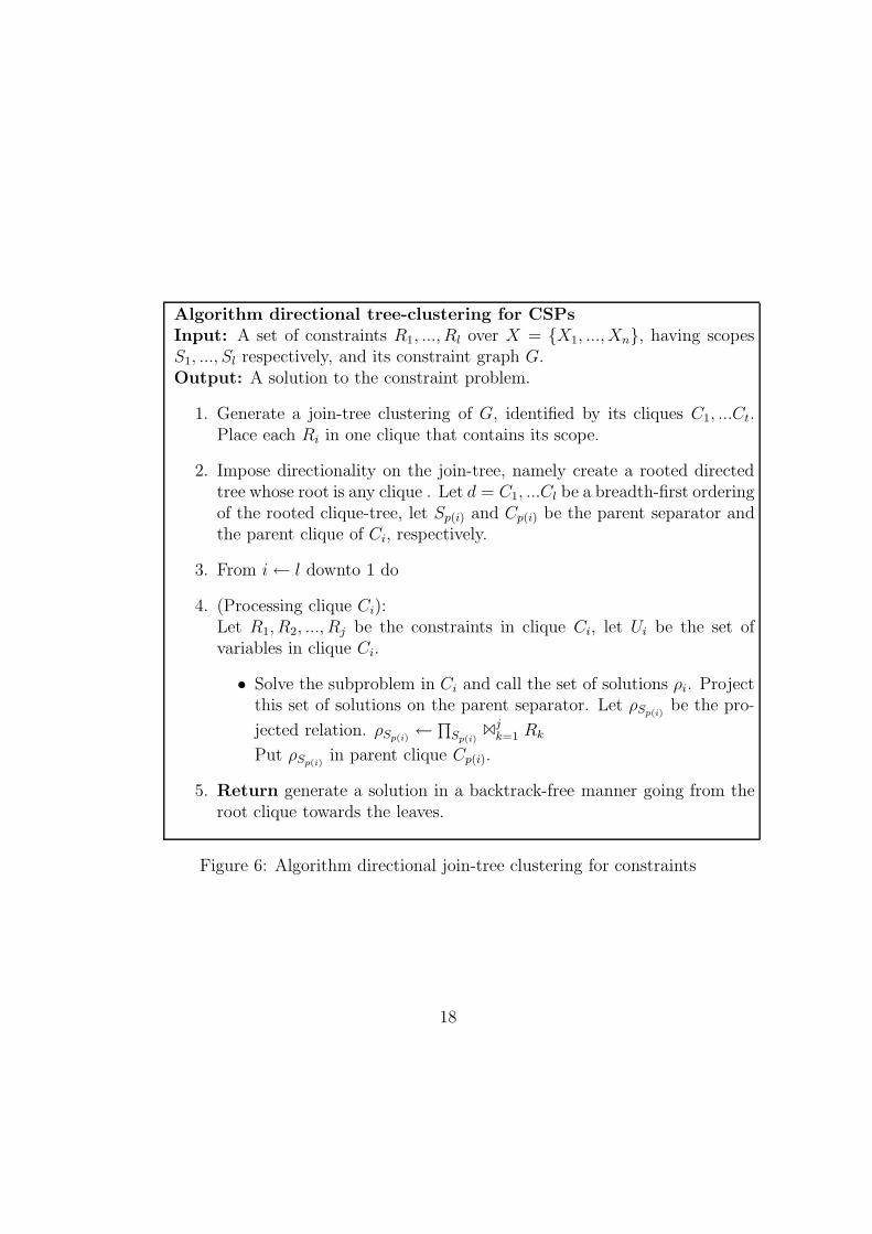
Algorithm directional tree-clustering for CSPsInput: A set of constraints R1, ..., Rl over X = {X1, ..., Xn}, having scopesS1, ..., Sl respectively, and its constraint graph G.Output: A solution to the constraint problem.
1. Generate a join-tree clustering of G, identified by its cliques C1, ...Ct.Place each Ri in one clique that contains its scope.
2. Impose directionality on the join-tree, namely create a rooted directedtree whose root is any clique . Let d = C1, ...Cl be a breadth-first orderingof the rooted clique-tree, let Sp(i) and Cp(i) be the parent separator andthe parent clique of Ci, respectively.
3. From i← l downto 1 do
4. (Processing clique Ci):Let R1, R2, ..., Rj be the constraints in clique Ci, let Ui be the set ofvariables in clique Ci.
• Solve the subproblem in Ci and call the set of solutions ρi. Projectthis set of solutions on the parent separator. Let ρSp(i)
be the pro-
jected relation. ρSp(i)← ∏
Sp(i)1
jk=1 Rk
Put ρSp(i)in parent clique Cp(i).
5. Return generate a solution in a backtrack-free manner going from theroot clique towards the leaves.
Figure 6: Algorithm directional join-tree clustering for constraints
18

Theorem 7: Let G be a constraint graph over n variables and let T be ajoin-tree with separator size s or less. Let cs be the largest minimal cycle-cutset3 in any subproblem in T . Then the problem can be solved in spaceO(n · exp(s)) and in time O(n · exp(cs + 2)), where cs ≥ s. 2
Example 4 : Applying the cycle-cutset method to each subproblem inT0, T1, T2 (see Figure 3), yields the same time-space tradeoffs as for the beliefnetwork case.
A special case of Theorem 7, observed before in [13, 17], occurs when thegraph is decomposed into non-separable components (i.e., when the separatorsize equals 1).
Corollary 1: If G has a decomposition to non-separable components suchthat the size of the maximal cutsets in each component is bounded by c, thenthe problem can be solved in O(n · exp(c)) time, using linear space. 2
4 Optimization Tasks
Clustering and conditioning are applicable also to optimization tasks definedover probabilistic and deterministic networks. An optimization task is de-fined relative to a real-valued criterion or cost function associated with everyinstantiation. In the context of constraint networks, the task is to find aconsistent instantiation having maximum cost. Applications include diagno-sis and scheduling problems. In the context of probabilistic networks, thecriterion function denotes a utility or a value function, and the task is to findan assignment to a subset of decision variables that maximize the expectedcriterion function. Applications include planning and decision making underuncertainty. If the criterion function is decomposable, its structure can beaugmented onto the corresponding graph to subsequently be exploited byeither tree-clustering or conditioning.
Definition 6 [Decomposable criterion function [3, 25]]: A criterion functionover a set X of n variables X1, ..., Xn having domains of values D1, ..., Dn isadditively decomposable relative to a scheme Q1, ..., Qt where Qi ⊆ X iff
f(x) =∑
i∈T
fi(xQi),
3As before, the cycle-cutset contains the separator set
19

where T = {1, ..., t} is a set of indices denoting the subsets of variables{Qi} and x is an instantiation of all the variables. The functions fi are thecomponents of the criterion function and are specified, in general, by storedtables.
Definition 7 [Constraint optimization, augmented graph] Given a constraintnetwork over a set of n variables X = X1, ...., Xn and a set of constraintsC1, ..., Ct having scopes S1, ..., St, and given a criterion function f decompos-able into {f1, ..., fl} over Q1, ..., Ql, the constraint optimization problem is tofind a consistent assignment x = (x1, ..., xn) such that the criterion functionf =
∑i fi, is maximized. The augmented constraint graph contains a node
for each variable and an arc connecting any two variables that appear eitherin the same scope of a constraint or in the same functional component of thecriterion function.
Since constraint optimization can be performed in linear time when theaugmented constraint graph is a tree, both join-tree clustering and cutset-conditioning can extend the method to non-tree structures [32] in the usualmanner. We can conclude:
Theorem 8: [32][Time-space of constraint optimization]: Given a constraintoptimization problem over n variables whose augmented constraint graph hasa cycle-cutset of size c, and whose augmented graph can be embedded in aclique-tree having tree width r and separator size s, the time complexity offinding an optimal consistent solution using tree-clustering is O(n · exp(r))and the space complexity O(n · exp(s)). The time complexity for finding aconsistent optimal solution using the cycle-cutset conditioning is O(n·exp(c))while its space complexity is linear. 2
In a similar manner, the structure of the criterion function can augmentthe moral graph when computing the maximum expected utility (MEU) ofsome decisions in a general influence diagram [20]. For more details see [12].
Once we have established the graph that guides tree-clustering and condi-tioning, the same principle of trading space for time becomes applicable andwill yield a collection of parameterized algorithms governed by the primaryand secondary clique-trees and cycle-cutsets of the augmented graphs as wehave seen before. For completeness sake we restate the full theorem:
20

C
A
B
D E
G F
H
G D E F
B G D G E F H
C D BA B G
B G
G D
B D
G E F
Figure 7: An augmented moral graph for the utility functionf(a, b, c, d, e, f, g.h) = a · g + c2 + 5d · e · f
Theorem 9: Given a constraint network over n variables and given an addi-tively decomposable criterion function f , if the augmented constraint graphrelative to the criterion function can be embedded in a clique-tree having sep-arator sizes s0, s1, ...sk, and corresponding maximal clique sizes r0, r1, ..., rk
and corresponding maximal minimal cutset sizes c0, c1, ..., ck, then finding anoptimal solution can be accomplished using any one of the following boundson the time and space: if a brute-force approach is used for processing eachsubproblem the bounds are O(n · exp(ri)) time and O(n · exp(si)) space. Ifcycle-cutset conditioning is used for each cluster, the bounds are O(n·exp(ci))time and O(n · exp(si)) space, where ci ≥ si. 2
Example 5: Consider the following criterion function defined over theconstraint network in Figure 5
u(a, b, c, d, e, f, g, h) = a · g + c2 + 5d · e · f.
Here the augmented graph will have one additional arc connecting nodesA and G (see Figure 7(a)), resulting in a primary clique-tree embedding inFigure 7(b) that differs from the tree in Figure 3(a). As a result one has toconsider the clique ABG instead of the original clique AB. Thus, applyingjoin-tree clustering to the primary tree yield time complexity O(exp(4)) andspace complexity O(k3). If only binary functions can be recorded we willneed to combine clique (GDEF ) with (GEFH) yielding a clique of size 5.Using cycle-cutset conditioning, this results in time complexity of O(k4) aswell, while using O(k2) space, only. If this space requirement is too heavy weneed to solve the whole problem as one cluster using cycle-cutset conditioningwhich, in this case, requires O(k5) time and linear space.
21

5 Empirical framework and results
The motivation for the experiments is twofold. One, to analyze the struc-tural parameters of clustering and cutset on real-life instances. Two, to gainfurther understanding of how space/time tradeoff can be exploited to alle-viate space bottlenecks. We analyzed empirically benchmark combinatorialcircuits, widely used in the fault diagnosis and testing community [6]. (SeeTable 1.) The experiments allow us to assess in advance the complexity ofdiagnosis and abduction tasks on those circuits, and to determine the appro-priate combination of tree clustering and cycle cutset methods to performthose tasks for each instance. None of the circuits are trees and they all haveconsiderable fanout nodes as shown in the schematic diagram of circuit c432in Fig. 8.
Table 1: ISCAS ’85 Benchmark Circuit Characteristics
Circuit Circuit Total Input OutputName Function Gates Lines LinesC17 6 5 2C432 Priority Decoder 160 (18 EXOR) 36 7C499 ECAT 202 (104 EXOR) 41 32C880 ALU and Control 383 60 26C1355 ECAT 546 41 32C1908 ECAT 880 33 25C2670 ALU and Control 1193 233 140C3540 ALU and Control 1669 50 22C5315 ALU and Selector 2307 178 123C6288 16-bit Multiplier 2406 32 32C7552 ALU and Control 3512 207 108
A directed acyclic graph (DAG), is computed for each circuit. The graphincludes a node for each variable in the circuit. For every gate in the circuit,the graph has an edge directed from each gate’s input to the gate’s output.The nodes with no parents (children) in the DAG are the primary inputs(outputs) of the circuit. The primal graph for each circuit is then computedas the moral graph for the corresponding DAG. Table 2 gives the number of
22

Figure 8: Schematic of circuit c432: 36 inputs 7 outputs and 160 components.
23

Table 2: Number of nodes and edges for the primal graphs of the circuits.
Circuit c17 c432 c499 c880 c1355 c1908 c2670 c3540 c5315 c6288 c7552#nodes 11 196 243 443 587 913 1426 1719 2485 2448 3719#edges 18 660 692 1140 1660 2507 3226 4787 7320 7184 9572
nodes and edges of the primal graph for each circuit.
Figure 9: Primary join tree (157 cliques) for circuit c432 (196 variables); themaximum separator size is 23.
Tree clustering is performed on the primal graphs as usual: by selectingan ordering for the nodes, then triangulating the graph and identifying itsmaximum cliques. There are many possible heuristics for ordering the nodeswith the aim of obtaining a join tree with small cliques.
Four ordering heuristics were considered: (1) causal ordering, (2) maximum-cardinality, (3) minimum-width, and (4) minimum-degree. The max-cardinalityordering is computed from first to last by picking the first node arbitrarily andthen repeatedly selecting the unordered node that is adjacent to the maxi-
24

mum number of already ordered nodes. The min-width ordering is computedfrom last to first by repeatedly selecting the node having the least numberof neighbors in the graph, removing the node and its incident edges from thegraph, and continuing until the graph is empty. The min-degree ordering [5]is exactly like min-width except that we connect neighbors of selected nodes,and the causal ordering is just a topological sort of the directed graph forthe circuit.
Tree clustering was implemented using each of the four orderings on eachof the benchmark circuits of Table 1 and we observed that the min-degreeordering was by far the best, yielding the smallest cliques sizes and separators.Our evaluation of the performance of the orderings is consistent with theresults in [23]. Therefore, we report here the results only relative to themin-degree ordering. For results on the other orderings see [12].
5.1 Results: Primary Join Trees
For each primary join tree generated, three parameters are computed: (1) thesize of cliques, (2) the size of cycle-cutsets in each of the subgraphs definedby the cliques, and (3) the size of the separator sets. The nodes of the jointree are labeled by the cliques (or clusters) sizes and the edges are labeledby the separator size. In this section we present the results on two circuitsc432 and c3540, having 196 and 1719 variables, respectively. Results on othercircuits are summarized in [12].
Figure 9 and 10 present information on the primary join trees. For ex-ample, Figure 9 shows that the cliques sizes range from 2 to 28. The rootnode has 28 nodes and the descendant nodes have strictly smaller sizes. Thedepth of the tree is 11 and all nodes whose distance from the root is greaterthan 6 have sizes strictly less than 10. The leaves have sizes ranging from2 to 6. The corresponding numbers for the primary join tree of the largercircuit c3540 shown in Fig. 10.
Figures 11 and 12 provide additional details showing the frequencies ofcliques sizes, separator sizes and cutsets sizes for both circuits. Those figures(and all the corresponding figures in [12])
show that the structural parameters are skewed with the vast majorityof the parameters having values below the midpoint (the point dividing therange of values from smallest to largest).
We see in Figure 11 that the number of cliques is 157 and the cliques sizes
25

Figure 10: Part of primary join tree (1419 cliques) for circuit c3540 (1719variables) showing the descendants of the root node down to the leaves; themaximum separator size is 89.
26

Frequencies
Cliq
ue s
ize
10 20 30 40
Clique sizes for c432Total number= 157,Maximum= 28Mode= 5,Median= 6,Mean= 7.43312
23456789
1011121719212728
Frequencies
Sep
arat
or w
idth
10 20 30 40
Separator widths for c432Total number= 156,Maximum= 23Mode= 4,Median= 5,Mean= 6.22436
1
2
3
4
5
6
7
8
9
10
11
16
18
20
23
Frequencies
Cut
set s
ize
20 40 60 80
Cutset sizes for c432Total number= 157,Maximum= 17Mode= 1,Median= 1,Mean= 1.92357
0
1
2
3
4
5
7
8
9
10
16
17
Figure 11: Histograms of the cliques sizes, the separator sizes and the cutsetssizes of the primary join tree for circuit c432 (196 variables)
Frequencies
Cliq
ue s
ize
100 200 300 400
Clique sizes for c3540Total number= 1419,Maximum= 114Mode= 4,Median= 5,Mean= 8.15645
2
3
4
5
6
7
8
9
10
11
12
13
14
Frequencies
Sep
arat
or w
idth
100 200 300 400 500
Separator widths for c3540Total number= 1418,Maximum= 89Mode= 3,Median= 4,Mean= 6.94993
1
2
3
4
5
6
7
8
9
10
11
12
13
Frequencies
Cut
set s
ize
100 200 300 400 500 600 700
Cutset sizes for c3540Total number= 1419,Maximum= 16Mode= 1,Median= 1,Mean= 1.32488
0
1
2
3
4
5
6
7
9
10
11
13
16
Figure 12: Histograms of the cliques sizes (0.9th quantile range), the separa-tor sizes (0.9th quantile range) and the cutsets sizes of the primary join treefor circuit c3540 (1719 variables).
27

are in the range from 2 to 28. The mode is 5, the median is 6 and the meanis 7.433. 40 cliques out of the total 157 have size 5, and only 23 out of 157have size greater than 9. The separator sizes are in the range from 1 to 23.The mode is 4, the median is 5 and the mean is 6.224. Out of the total 156separator sizes, 40 have size 4 and only 13 have sizes greater than 10. Thecutsets sizes are in the range from 0 to 17. The mode is 1, the median is 1and the mean is 1.923. Out of 157 cliques, 23 have cutset size 0. This meansthat the projection of the primal graph on each of those 23 cliques is alreadyacyclic.
The corresponding figures for C3540 can be read from Figure 12. Fig-ure 12 shows the 0.9th quantile distribution of the separator sizes. Likethe cliques, 90% of the separator sizes are small (between 1 and 13) andthe remaining 10% span a broad range of values (from 14 to 89). For thecutsets sizes we note that 318 cutsets out of total 1419 have size 0, namelythe projection on each of those 318 cliques is already acyclic. We also notethat 753 out of 1419 cliques have singleton cutsets. Only 47 out of 1419cutsets have sizes greater than 5.
5.2 Results: Hybrid Clustering + Conditioning
As we see, some cliques and separators require memory space exponential in23 for circuit c432 and exponential in 89 for circuit c3540. This is clearly notfeasible. We will next evaluate the potential of the trade off scheme proposedin this paper.
Let s0, c0 be the maximum cutset and separator size of the primaryjoin tree T0 obtained by tree clustering. Let s0, s1, . . . , sn be the size of theseparators in T0 listed from largest to smallest. As explained earlier, witheach separator size, si, we associate a tree decomposition Ti generated bycombining adjacent clusters whose separators’ sizes are strictly larger thansi. We denote by ci the largest cutset size in any cluster of Ti.
We estimate the space/time bounds for each circuit based on the graphparameters observed using our tree decomposition scheme. Figure 13 gives achart presenting bounds for time versus space for each circuit. Each point inthe chart corresponds to a specific secondary join tree decomposition Ti andhas the space complexity measured by the separator size, si, and the timecomplexity by the maximum between the separator size and the cutset size;max(si, ci).
28

10 20 30 40
Space
50100150200250300
Time
Circuit c1908
0 5 10 15 20 25 30
Space
100
200
300
400
Time
Circuit c2670
0 5 10 15 20
Space
20406080100120140160
Time
Circuit c880
2.5 5 7.5 1012.51517.5
Space
50
100
150
200Time
Circuit c1355
5 10 15 20
Space
20304050607080
Time
Circuit c432
2.5 5 7.5 1012.51517.5
Space
203040506070
Time
Circuit c499
Figure 13: Time/Space tradeoff for c432 (196 variables), c499 (243 variables),c880 (443 variables), c1355 (587 variables), c1908 (913 variables) and c2670(1426 variables). Time is measured by the maximum of the separator sizeand the cutset size and space by the maximum separator size.29

Each chart in Figure 13 can be used to select the algorithm from thespectrum of conditioning+clustering algorithms of our tree decompositionscheme that best meets a given time-space specification. They show thegradual effect of lowering space on the time required by a correspondingclustering+conditioning algorithm. For example circuit c432 (Figure 13)shows the separator size (space) which is initially 23 (for the primary jointree) gradually reduced down to 1 in a series of secondary trees. The figuredemonstrates that reducing the separator size (to meet the space restrictions)increases the worst-case time complexity of the hybrid algorithm. The timeincreases because of the large clusters contained in the secondary join treeand the corresponding increase in the size of cutsets.
Note that the charts in Figure 13 all display a “knee” phenomenon inthe time-space tradeoff where time increases only slightly for a wide range ofspace reduction beyond which further reduction in space causes significantrise in the time bound. Note also that the time estimate shown in Figure 13displays a small dip before it rises with the decrease in available space. Forexample for circuit c432 we note a dip when the space is decreased from 23to 20.
Figures 14 and 15 display the structure of secondary join trees for c432.The primary join tree for the circuit is shown in Figure 9. The secondarytrees are indexed by the separator sizes of the primary tree which range from1 to 23 (Figure 11). As the separator decreases the maximum clique sizeincreases, and both the size and the depth of the tree decrease. Like theprimary join tree, each secondary join tree has also a skewed distribution ofthe clique sizes. Note that the clique size for the root node is significantlylarger than for all other nodes, and is increasing as the separator decreases.
6 Related work
The cycle-cutset scheme for probabilistic inference was introduced by Pearl[29] and for constraint networks by Dechter [8]. It was further improved andextended for probabilistic reasoning by [30, 7, 15].
In subsequent years the cycle-cutset scheme was recognized as a specialcase of conditioning, namely, value assignments to a subset of variables cre-ates subproblems that can be solved by any means. While the cycle-cutsetscheme requires that the conditioning set will be large enough so that the
30

Figure 14: Secondary trees for c432 with separator sizes 16 and 11
31

Figure 15: Secondary trees for c432 with separator sizes 7 and 3.
resulting subproblem is singly-connected, any size of conditioning set can beused, yielding simplified problems that can be solved by tree-clustering or byany other method. This idea of extending the combination of conditioningand tree-clustering beyond the cycle-cutset scheme appears in the work ofJegou [21] for constraint networks and in the works of [31, 19] for probabilis-tic networks. In the work of Jegou various heuristic are presented, aimingat creating a hybrid algorithm having improved time performance. In [31],the issue of reducing the space of tree-clustering by combination with con-ditioning is also briefly addressed. The latter paper includes an alternativeproof to the (worst-case) time superiority of tree-clustering over the cycle-cutset method. In [19] the idea is applied to the pathfinder system, whenthe conditioning set is restricted to the set of diseases.
Finally in [33, 34], a scheme for combining conditioning and variableelimination for propositional theories is outlined and analyzed. It is shownthat although the worst-case time guarantee of an hybrid cannot be superiorto tree-clustering (nor to a variable elimination scheme), for some problemclasses a hybrid algorithm can have a better time performance than both pureclustering and pure search. The work in this paper provides an alternative
32

hybrid scheme between conditioning and elimination.
7 Summary and Conclusions
Problem solving methods can be viewed as hybrids of two main principles:inference and search. Tree-clustering is an example of an inference algorithmwhile the cycle-cutset is an example of a search method. Tree clustering algo-rithms are time and space exponential in the size of their cliques while searchalgorithms are time exponential but require only linear memory. In this pa-per we developed a structure-based hybrid scheme that uses tree-clusteringand cycle-cutset conditioning as its two extremes and, using a single designparameter, permits the user to control and tailor the storage-time tradeoffin accordance with the problem domain and the available resources
Specifically, we have shown that constraint processing and belief networkprocessing obey a structure-based time-space tradeoff, that allows tailoring acombination of tree-clustering and cycle-cutset conditioning to certain timeand space requirements. As well, the same tradeoff is obeyed by optimizationproblems when augmenting the graph by arcs reflecting the structure of thecriterion function. Our analysis presents a spectrum of algorithms that allowsa rich time-space performance balance, applicable across a variety of tasks.
The structural parameters of interest are: (1) the size of cliques in a jointree, namely, the induced-width, (2) the size of cycle-cutsets in each of thesubgraphs defined by the cliques, and (3) the size of the separator sets.
To assess the applicability of our scheme to real-life domains, we studiedthe structural parameters of 11 benchmark circuits widely used in the faultdiagnosis and testing community [6]. We observed that the join-trees ofthe circuits all shared the unexpected property that while few cliques aredistinctly large, the majority of cliques sizes are relatively small. Also, thedistributions of all the structural parameters are skewed. This observationhas an important practical implication. Although the primary join tree ob-tained by tree-clustering may require too much space, a major portion of thetree can be solved without any space problem.
Our analysis should be qualified, however. All the results present worst-case guarantees of the corresponding algorithm. It is still not clear thatthe bounds are tight nor that they correlate with average case performance.This analysis should be extended in the future to include implementing and
33

testing of the involved algorithms, a major effort outside the scope of thispaper.
References
[1] S. Arnborg and A. Proskourowski. Linear time algorithms for np-hardproblems restricted to partial k-trees. Discrete and Applied Mathemat-ics, 23:11–24, 1989.
[2] S. A. Arnborg. Efficient algorithms for combinatorial problems on graphswith bounded decomposability - a survey. BIT, 25:2–23, 1985.
[3] F. Bacchus and P. van Run. Dynamic variable ordering in csps. InPrinciples and Practice of Constraints Programming (CP’95), Cassis,France, 1995. Available as Lecture Notes on CS, vol 976, pp 258 – 277,1995.
[4] A. Becker and D. Geiger. A sufficiently fast algorithm for finding closeto optimal junction trees. In Uncertainty in AI (UAI’96), pages 81–89,1996.
[5] U. Bertele and F. Brioschi. Nonserial Dynamic Programming. AcademicPress, 1972.
[6] Brglez and Fujiwara. A neutral netlist of 10 combinatorial benchmarkcircuits and a target translator in fortran. In Proceedings of the IEEEInternational Symposium on Circuits and Systems, 1996.
[7] A Darwiche. Conditioning algorithms for exact and approximate infer-ence in causal networks. In Uncertainty in Artificial Intelligence (UAI-95), pages 99–107, 1995.
[8] R. Dechter. Enhancement schemes for constraint processing: Backjump-ing, learning and cutset decomposition. Artificial Intelligence, 41:273–312, 1990.
[9] R. Dechter. Constraints networks. In Encyclopedia of Artificial Intelli-gence, 2nd Ed., pages 276–285, 1992.
34

[10] R. Dechter. Bucket elimination: A unifying framework for probabilisticinference algorithms. In Uncertainty in Artificial Intelligence (UAI’96),pages 211–219, 1996.
[11] R. Dechter. Bucket elimination: A unifying framework for reasoning.Artificial Intelligence, 113:41–85, 1999.
[12] R. Dechter and Y. El Fattah. Topological parameters for time-spacetradeoff. Technical report, 1999.
[13] R. Dechter and J. Pearl. Network-based heuristics for constraint satis-faction problems. Artificial Intelligence, 34:1–38, 1987.
[14] R. Dechter and J. Pearl. Tree clustering for constraint networks. Arti-ficial Intelligence, pages 353–366, 1989.
[15] F. J. Diez. Local conditioning in bayesian networks. Artificial Intelli-gence, 87:1–20, 1996.
[16] Y. El Fattah and R. Dechter. Diagnosing tree-decomposable circuits.In International Joint Conference of Artificial Intelligence (IJCAI-95),pages 1742–1748, Montreal, Canada, August 1995.
[17] E. C. Freuder. A sufficient condition for backtrack-free search. Journalof the ACM, 29(1):24–32, 1982.
[18] H. Geffner and J. Pearl. An improved constraint propagation algorithmfor diagnosis. In Proceedings of IJCAI-87, pages 1105–1111, Milan, Italy,1987.
[19] G. F. Cooper H. J. Suermondt and D. E. Heckerman. A combinationof cutset conditioning with clique-tree propagation in the path-findersystem. In Uncertainty in Artificial Intelligence (UAI’91), pages 245–253, 1991.
[20] R. A. Howard and J. E. Matheson. Influence diagrams. 1984.
[21] P Jegou. Cyclic clustering: a compromise between tree-clustering andthe cycle-cutset method for improving search efficiency. In EuropeanConference on AI (ECAI-90), pages 369–371, Stockholm, 1990.
35

[22] F.V. Jensen, S.L Lauritzen, and K.G. Olesen. Bayesian updating incausal probabilistic networks by local computation. ComputationalStatistics Quarterly, 4:269–282, 1990.
[23] U. Kjæaerulff. Triangulation of graph-based algorithms giving smalltotal state space. In Technical Report 90-09, Department of Mathematicsand computer Science.
[24] U. Kjæaerulff. Nested junction trees. In Uncertainty in Artificial Intel-ligence (UAI’97), pages 294–301, 1997.
[25] D. H. Krantz, R.D. Luce, P. Suppes, and A. Tversky. Foundations ofmeasurements, academic press. 1976.
[26] S.L. Lauritzen and D.J. Spiegelhalter. Local computation with proba-bilities on graphical structures and their application to expert systems.Journal of the Royal Statistical Society, Series B, 50(2):157–224, 1988.
[27] A. K. Mackworth and E. C. Freuder. The complexity of some polynomialnetwork consistency algorithms for constraint satisfaction problems. Ar-tificial Intelligence, 25, 1985.
[28] J. Pearl. Fusion propagation and structuring in belief networks. ArtificialIntelligence, 29(3):241–248, 1986.
[29] J. Pearl. Probabilistic Reasoning in Intelligent Systems. Morgan Kauf-mann, 1988.
[30] M. A. Peot and R. D. Shachter. Fusion and proagation with multipleobservations in belief networks. Artificial Intelligence, pages 299–318,1992.
[31] S.K. Anderson R. D. Shachter and P. Solovitz. Global conditioning forprobabilistic inference in belief networks. In Uncertainty in ArtificialIntelligence (UAI’94), pages 514–522, 1994.
[32] A. Dechter R. Dechter and J. Pearl. Optimization in constraint networks.In Influence Diagrams, Belief Nets and Decision Analysis, pages 411–425. John Wiley & Sons, 1990.
36

[33] I. Rish and R. Dechter. To guess or to think? hybrid algorithms forsat. In Principles of Constraint Programming (CP-96), pages 555–556,1996.
[34] I. Rish and R. Dechter. Resolution vs. sat: two approaches to sat.Journal of Approximate Reasoning (to appear), 2000.
[35] D. G. Corneil S. A. Arnborg and A. Proskourowski. Complexity offinding embeddings in a k-tree. SIAM Journal of Discrete Mathematics.,8:277–284, 1987.
[36] T. Schmidt and P.P. Shenoy. Some improvements to the shenoy-shaferand hugin architecture for computing marginals. Artificial Intelligence,102:323–333, 1998.
[37] G. Shafer. Probabilistic expert systems. Society for indutrial and AppliedMathematics, Philadelphia, PA, 1996.
[38] G. R. Shafer and P.P. Shenoy. Probability propagation. Anals of Math-ematics and Artificial Intelligence, 2:327–352, 1990.
[39] K. Shoiket and D. Geiger. A proctical algorithm for finding optimal tri-angulations. In Fourteenth National Conference on Artificial Intelligence(AAAI’97), pages 185–190, 1997.
[40] S. Srinivas. A probabilistic approach to hierarchical model-based diagno-sis. In Working Notes of the Fifth International Workshop on Principlesof Diagnosis, pages 305–311, New Paltz, NY, USA, 1994.
37