Embed Size (px)
Citation preview
Acta Numericahttp://journals.cambridge.org/ANU
Additional services for Acta Numerica:
Email alerts: Click hereSubscriptions: Click hereCommercial reprints: Click hereTerms of use : Click here
Topological pattern recognition for point cloud data
Gunnar Carlsson
Acta Numerica / Volume 23 / May 2014, pp 289 - 368DOI: 10.1017/S0962492914000051, Published online: 12 May 2014
Link to this article: http://journals.cambridge.org/abstract_S0962492914000051
How to cite this article:Gunnar Carlsson (2014). Topological pattern recognition for point cloud data . Acta Numerica, 23,pp 289-368 doi:10.1017/S0962492914000051
Request Permissions : Click here
Downloaded from http://journals.cambridge.org/ANU, IP address: 171.67.216.22 on 18 Jul 2014

Acta Numerica (2014), pp. 289–368 c© Cambridge University Press, 2014
doi:10.1017/S0962492914000051 Printed in the United Kingdom
Topological pattern recognitionfor point cloud data∗
Gunnar Carlsson†
Department of Mathematics,
Stanford University,
CA 94305, USA
E-mail: [email protected]
In this paper we discuss the adaptation of the methods of homology fromalgebraic topology to the problem of pattern recognition in point cloud datasets. The method is referred to as persistent homology, and has numerousapplications to scientific problems. We discuss the definition and computationof homology in the standard setting of simplicial complexes and topologicalspaces, then show how one can obtain useful signatures, called barcodes, fromfinite metric spaces, thought of as sampled from a continuous object. Wepresent several different cases where persistent homology is used, to illustratethe different ways in which the method can be applied.
CONTENTS
1 Introduction 2892 Topology 2933 Shape of data 3114 Structures on spaces of barcodes 3315 Organizing data sets 343References 365
1. Introduction
Deriving knowledge from large and complex data sets is a fundamental prob-lem in modern science. All aspects of this problem need to be addressedby the mathematical and computational sciences. There are various dif-ferent aspects to the problem, including devising methods for (a) storingmassive amounts of data, (b) efficiently managing it, and (c) developing un-derstanding of the data set. The past decade has seen a great deal of devel-opment of powerful computing infrastructure, as well as methodologies for
∗ Colour online for monochrome figures available at journals.cambridge.org/anu.† Research supported in part by the National Science Foundation, the National Institutesof Health, and the Air Force Office of Scientific Research.

290 G. Carlsson
1
2
3
4
5
6
Figure 1.1. A compressed combinatorial representation of a circle.
managing and querying large databases in a distributed fashion. In thispaper, we will be discussing one approach to (c) above, that is, to the prob-lem of generating knowledge and understanding about large and complexdata sets.Much of mathematics can be characterized as the construction of methods
for organizing infinite sets into understandable representations. Euclideanspaces are organized using the notions of vector spaces and affine spaces,and this allows us to organize the (infinite) underlying sets into understand-able objects which can be readily manipulated, and which can be used toconstruct new objects from old in systematic ways. Similarly, the notion ofan algebraic variety allows us to work effectively with the zero sets of setsof polynomials in many variables. The notion of shape is similarly encodedby the notion of a metric space, a set equipped with a distance function sat-isfying three simple axioms. This abstract notion permits us to study notonly ordinary notions of shape in two and three dimensions but also higher-dimensional analogues, as well as objects such as the p-adic integers, whichare not immediately recognized as being geometric in character. Thus, thenotion of a metric serves as a useful organizing principle for mathemati-cal objects. The approach we will describe demonstrates that the notion ofmetric spaces acts as an organizing principle for finite but large data setsas well.Topology is one of the branches of mathematics which studies properties
of shape. The study of shape particular to topology can be described interms of three points.
(1) The properties of shape studied by topology are independent of anyparticular coordinate representation of the shape in question, and in-stead depend only on the pairwise distances between the points makingup the shape.
(2) Topological properties of shape are deformation invariant, that is, theydo not change if the shape is stretched or compressed. They would ofcourse change if non-continuous transformations were applied, ‘tearing’the space.
Topological pattern recognition for point cloud data 291
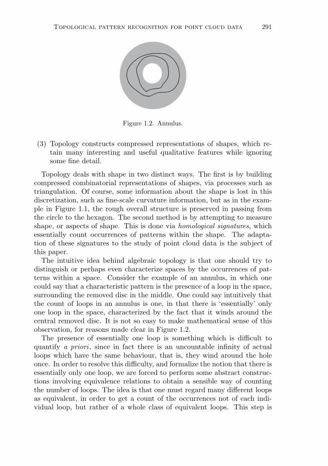
Figure 1.2. Annulus.
(3) Topology constructs compressed representations of shapes, which re-tain many interesting and useful qualitative features while ignoringsome fine detail.
Topology deals with shape in two distinct ways. The first is by buildingcompressed combinatorial representations of shapes, via processes such astriangulation. Of course, some information about the shape is lost in thisdiscretization, such as fine-scale curvature information, but as in the exam-ple in Figure 1.1, the rough overall structure is preserved in passing fromthe circle to the hexagon. The second method is by attempting to measureshape, or aspects of shape. This is done via homological signatures, whichessentially count occurrences of patterns within the shape. The adapta-tion of these signatures to the study of point cloud data is the subject ofthis paper.The intuitive idea behind algebraic topology is that one should try to
distinguish or perhaps even characterize spaces by the occurrences of pat-terns within a space. Consider the example of an annulus, in which onecould say that a characteristic pattern is the presence of a loop in the space,surrounding the removed disc in the middle. One could say intuitively thatthe count of loops in an annulus is one, in that there is ‘essentially’ onlyone loop in the space, characterized by the fact that it winds around thecentral removed disc. It is not so easy to make mathematical sense of thisobservation, for reasons made clear in Figure 1.2.The presence of essentially one loop is something which is difficult to
quantify a priori , since in fact there is an uncountable infinity of actualloops which have the same behaviour, that is, they wind around the holeonce. In order to resolve this difficulty, and formalize the notion that there isessentially only one loop, we are forced to perform some abstract construc-tions involving equivalence relations to obtain a sensible way of countingthe number of loops. The idea is that one must regard many different loopsas equivalent, in order to get a count of the occurrences not of each indi-vidual loop, but rather of a whole class of equivalent loops. This step is

292 G. Carlsson
what is responsible for much of the abstraction which is introduced into thesubject. Once that layer of abstraction has been built, it provides a wayto detect the presence of geometric patterns of certain types. The generalidea of a pattern is of course a diffuse one, with many different meaningsin many different contexts. In the geometric context, we define patterns asmaps from a template space, such as a circle, into the space. A large partof the subject concerns the process of reducing the abstract constructionsdescribed above to much more concrete mathematical constructions, involv-ing row and column operations on matrices. The goals of the present paperare as follows.
• To introduce the pattern detection signatures which come up in al-gebraic topology, and simultaneously to develop the matrix methodswhich make them into computable and usable invariants for variousgeometric problems, particularly in the domain of point clouds or fi-nite metric spaces. We hope that the introduction of the relevantmatrix algorithms will begin to bridge the gap between topology aspractised ‘by hand’, and the computational world. We will describethe standard methods of homology, which attach a list of non-negativeintegers (called the Betti numbers) to any topological space, and alsothe adaptation of homology to a tool for the study of point clouds.This adaptation is called persistent homology.
• To introduce the mathematics surrounding the collection of persistencebarcodes or persistence diagrams, which are the values taken by thepersistent homology constructions. Unlike the Betti numbers, whichare integer-valued, persistent homology takes its values in multisetsof intervals on the real line. As such, they have a mix of continuousand discrete structure. The study of these spaces from various pointsof view, so as to be able to make them maximally useful in variousproblem domains, is one of the most important research directionswithin applied topology.
• To describe various examples of applications of persistent homologyto various problem domains. There are two distinct directions of ap-plication, one being the study of homological invariants of individualdata sets, and the other being the use of homological invariants in thestudy of databases where the data points themselves have geometricstructure. In this case, the barcode space can act as the home for akind of non-linear indexing for such databases.

Topological pattern recognition for point cloud data 293
A
B
C
D
Figure 2.1. Euler’s ‘Bridges of Konigsberg’ problem.
2. Topology
2.1. History
Euler’s paper of 1741, in which he studies the so-called ‘Bridges of Konigs-berg’ problem, is usually cited as the first paper in topology. The questionhe asked was whether it was possible to traverse all the bridges exactlyonce and return to one’s starting point. Euler answered this question byrecognizing that it was a question about paths in an associated network:see Figure 2.1. In fact, the question only depends on certain propertiesof the paths, independent of the rates at which the paths are traversed.His result concerned the properties of an infinite class of paths, or of acertain type of pattern in the network. Euler also derived Euler’s polyhe-dral formula, relating the number of vertices, edges and faces in polyhedra(Euler 1758a, 1758b). The subject developed in a sporadic fashion over thenext century and a half, including work by Vandermonde on knot theory(Vandermonde 1774), the proof of the Gauss–Bonnet theorem (never pub-lished by Gauss, but with a special case proved by Bonnet (1848)), the firstbook on the subject by Listing (1848), and the work of Riemann (1851)identifying the notion of a manifold. In 1895, Poincare published his sem-inal paper in which the notions of homology and fundamental group wereintroduced, with motivation from celestial mechanics. The subject then de-veloped at a greatly accelerated pace throughout the twentieth century. Thefirst paper on persistent homology was published by Robins (1999), and thesubject of applying topological methodologies to finite metric spaces hasbeen developing rapidly since that time.
2.2. Equivalence relations
A (binary) relation on a set X is a subset of X ×X. We will often denoterelations by ∼, and write x ∼ x′ to indicate that (x, x′) is in the relation.

294 G. Carlsson
Definition 2.1. A relation ∼ on a set X is an equivalence relation if thefollowing three conditions hold:
(1) x ∼ x for all x ∈ X,
(2) x ∼ x′ if and only if x′ ∼ x,
(3) x ∼ x′ and x′ ∼ x′′ implies x ∼ x′′.
By the equivalence class of x ∈ X, denoted by [x], we will mean the set
{x′| x ∼ x′}.The sets [x] for all x ∈ X form a partition of the setX. If∼ is any symmetricbinary relation on a set X, then by the equivalence relation generated by∼ (or the transitive closure of ∼) we will mean the equivalence relation∼′ defined by the condition that x0 ∼′ x1 if and only if there is a positiveinteger n and a sequence of elements x′0, x′1, . . . , x′n so that x′0 = x0, x
′n = x1,
and x′i ∼ x′i+1 for all 0 ≤ i ≤ n− 1.
For a set X and an equivalence relation ∼ on X, we will denote the setof equivalence classes under ∼ by X/ ∼, and refer to it as the quotientof X with respect to ∼. There are several important special cases of thisdefinition. The first is the quotient of a vector space by a subspace. Let Vbe a vector space over a field k, and let W ⊆ V be a subspace. We define anequivalence relation ∼W on V by setting v ∼W v′ if and only if v− v′ ∈W .It is easy to verify that ∼W is an equivalence relation. We can form thequotient V/ ∼W , and one observes that V/ ∼W is itself naturally a vectorspace over k, with the addition and scalar multiplication rules satisfying[v] + [v′] = [v + v′] and κ[v] = [κv]. In this special case, we will denoteV/ ∼W by V/W , and refer to it as the quotient space of V by W . Althoughthe quotient is an apparently abstract concept, it can be described explicitlyin a couple of ways.
Proposition 2.2. Suppose that we have a basis B of a vector space V ,and B′ ⊆ B is a subset. If W is the subspace of V spanned by B′, then thequotient V/W has the elements {[b]|b /∈ b′} as a basis, so the dimension ofV/W is #(B)−#(B′). More generally, if W ′ is a complement to W in V ,so that W +W ′ = V , and W ∩W ′ = {0}, then the composite
W ′ ↪→ Vp→ V/W
is a bijective linear transformation, so the dimension of V/W is equal to thedimension of W ′, where p is the map which assigns to v ∈ V its equivalenceclass [v] under ∼W .
There is also a matrix interpretation. Let V and W be vector spaces withordered bases, and let f : V → W be a linear transformation, with matrix

Topological pattern recognition for point cloud data 295
A(f) associated to the given bases. The image of f is a subspace of W ,and we write θ(f) for the quotient space W/im(f).
Proposition 2.3. Let g : V → V and h : W → W be invertible lineartransformations. Then θ(f) is isomorphic to θ(hfg). It follows that if wehave the matrix equation A(f ′) = A(h)A(f)A(g), then θ(f ′) is isomorphicto θ(hfg).
Proof. This follows from the elementary observation that w ∼im(f) w′ ifand only if
h(w) ∼im(hf) h(w′).
Proposition 2.4. Let W be the vector space km for some m, and supposethat we are given an m × n-matrix A with entries in a field k. A can beregarded as a linear transformation from V = kn to W , and the span of thecolumns in this matrix is the image of the transformation A. Then, if weapply any row or column operation (permuting rows/columns, multiplyinga row/column by a non-zero element of k, or adding a multiple of onerow/column to another) to obtain a matrix A
′, then θ(A) is isomorphic
to θ(A′).
Remark 2.5. Note that for any matrix A over a field, one can apply rowand column operations to bring it to the form[
In 00 0
],
where n is the rank of A. In this case, the dimension of the quotient isreadily computed using Proposition 2.2.
The second special case is that of the orbit set of a group action. If G isa group, and we have an action of G on a set X, then the action defines anequivalence relation ∼G on X by x ∼G x′ if there is a g ∈ G so that gx = x′.This is readily seen to be an equivalence relation, and the equivalence classesare called the orbits of the action.Finally, consider the case of a topological space X equipped with an
equivalence relation R. Then the quotient set X/R is equipped with atopology by declaring that a set U ⊆ X/R is open if and only if π−1(U) isan open set in X, where π : X → X/R is the map which assigns to eachx ∈ X its equivalence class [x].
2.3. Homotopy
The fundamental idea of algebraic topology is that one should develop meth-ods for counting the occurrences of geometric patterns in a topological spacein order to distinguish it from other spaces, or to suggest similarities be-tween different spaces. A simple example of this notion is given in Figure 2.2.
296 G. Carlsson
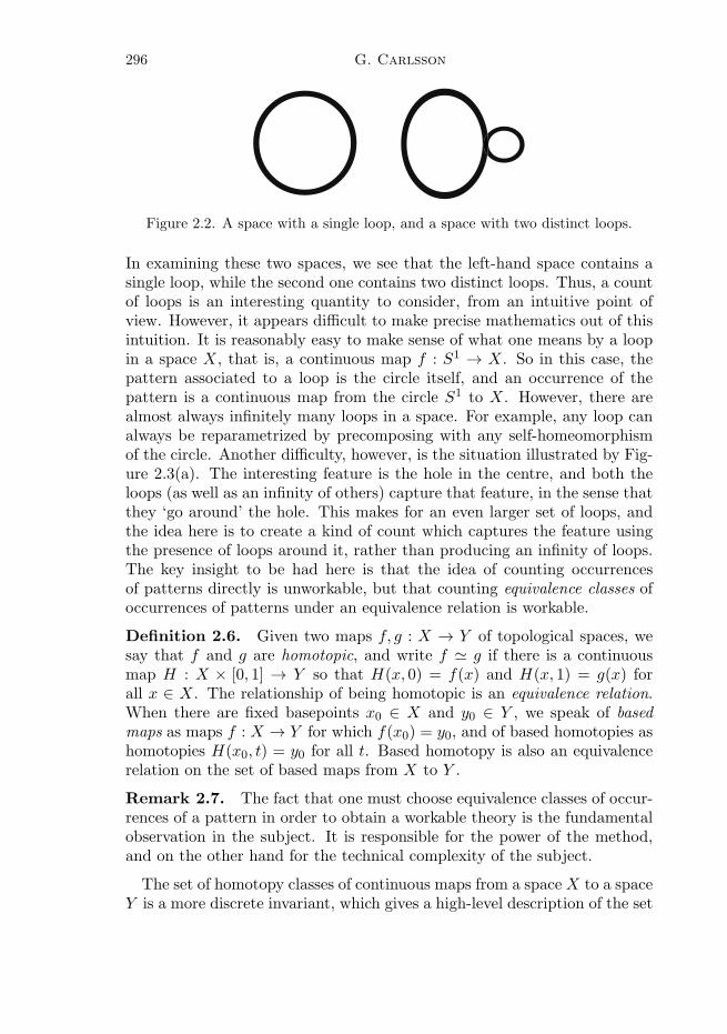
Figure 2.2. A space with a single loop, and a space with two distinct loops.
In examining these two spaces, we see that the left-hand space contains asingle loop, while the second one contains two distinct loops. Thus, a countof loops is an interesting quantity to consider, from an intuitive point ofview. However, it appears difficult to make precise mathematics out of thisintuition. It is reasonably easy to make sense of what one means by a loopin a space X, that is, a continuous map f : S1 → X. So in this case, thepattern associated to a loop is the circle itself, and an occurrence of thepattern is a continuous map from the circle S1 to X. However, there arealmost always infinitely many loops in a space. For example, any loop canalways be reparametrized by precomposing with any self-homeomorphismof the circle. Another difficulty, however, is the situation illustrated by Fig-ure 2.3(a). The interesting feature is the hole in the centre, and both theloops (as well as an infinity of others) capture that feature, in the sense thatthey ‘go around’ the hole. This makes for an even larger set of loops, andthe idea here is to create a kind of count which captures the feature usingthe presence of loops around it, rather than producing an infinity of loops.The key insight to be had here is that the idea of counting occurrencesof patterns directly is unworkable, but that counting equivalence classes ofoccurrences of patterns under an equivalence relation is workable.
Definition 2.6. Given two maps f, g : X → Y of topological spaces, wesay that f and g are homotopic, and write f � g if there is a continuousmap H : X × [0, 1] → Y so that H(x, 0) = f(x) and H(x, 1) = g(x) forall x ∈ X. The relationship of being homotopic is an equivalence relation.When there are fixed basepoints x0 ∈ X and y0 ∈ Y , we speak of basedmaps as maps f : X → Y for which f(x0) = y0, and of based homotopies ashomotopies H(x0, t) = y0 for all t. Based homotopy is also an equivalencerelation on the set of based maps from X to Y .
Remark 2.7. The fact that one must choose equivalence classes of occur-rences of a pattern in order to obtain a workable theory is the fundamentalobservation in the subject. It is responsible for the power of the method,and on the other hand for the technical complexity of the subject.
The set of homotopy classes of continuous maps from a space X to a spaceY is a more discrete invariant, which gives a high-level description of the set

Topological pattern recognition for point cloud data 297
(a) (b)
Figure 2.3. (a) Two equivalent loops. (b) Distinct equivalence classes of loops.
of maps from X to Y . When X is the n-sphere Sn, one can in a natural wayimpose the structure of a group on the set of equivalence classes of basedmaps from Sn to Y . The resulting group is denoted by πn(Y, y0). Appliedto the example above, with a single obstacle in the plane, this group π1 isa single copy of the integers with addition as the operation. The integerassigned to a given loop is the so-called winding number of the loop, whichcounts how many times the loop wraps around the obstacle, with orientationtaken into account as a sign.In Figure 2.3(b) the black loop has winding number +2, and the white
loop has winding number −1. If there were two obstacles, π1 would be a freenon-commutative group on two generators, and similarly n generators withn obstacles. If we had a three-dimensional region, with a single ball-shapedobstacle, then π1 would be trivial, but π2 would be identified with a copy ofthe integers, the invariant integer given by a higher-dimensional version ofthe winding number. The groups πn(Y, y0) are referred to as the homotopygroups of a space Y . They serve as a form of pattern recognition for thespace, in that they detect occurrences of the pattern corresponding to then-spheres. The homotopy groups allow us to distinguish between spaces,as follows.
Definition 2.8. Two topological spaces X and Y are said to be homotopyequivalent if there are continuous maps f : X → Y and g : Y → X such thatgf and fg are homotopic to the identity maps on X and Y , respectively.There is a corresponding notion for based maps and based homotopies.
Remark 2.9. We note that this is simply a ‘softened’ version of the usualnotion of isomorphism, where the composites are required to be equal to thecorresponding identity maps. Of course, spaces which are actually homeo-morphic are always homotopy equivalent.
It is now possible to prove the following.

298 G. Carlsson
Proposition 2.10. Suppose that two spaces X and Y are based homo-topy equivalent, with base points x0 and y0 as base points. Then all theirhomotopy groups πn(X,x0) and πn(Y, y0) are isomorphic.
This result often allows us to conclude that two spaces are not homotopyequivalent, and a fortiori not homeomorphic. For example, π2(S
2, 0) isisomorphic to the group of integers, while π2(R
2, 0) is isomorphic to thetrivial group, and we may conclude that they are not homotopy equivalent.Although they are easy to define and conceptually very attractive, it turns
out that homotopy groups of spaces are very difficult to compute. There isanother kind of invariant, called homology, which, instead of being easy todefine and difficult to compute, is difficult to define and easy to compute.
2.4. Homology
Homology was initially defined not for topological spaces directly, but ratherfor spaces described in a very particular way, namely as simplicial com-plexes. This description is very combinatorial, and it turns out that (a)not every space can be described as a simplicial complex, and (b) spacescan be described as simplicial complexes in many different ways. In theearly development of the subject, the apparent dependence of the homol-ogy calculation on the simplicial complex structure was a serious problem,and it was the subject of a great deal of research. These problems wereeventually resolved by Eilenberg, who showed that there is a way to extendthe definition of homology groups to all spaces, and in such a way that theresult depends only on the space itself and not on any particular structuresas a simplicial complex. Eilenberg’s solution was, however, extremely in-finite in nature, and is not amenable to direct computation. Calculationsof homology for simplicial complexes remain the best method for explicitcalculation. Because most spaces of interest are either explicitly simpli-cial complexes or homotopy equivalent to such complexes, it turns out thatsimplicial calculation is sufficient for most situations.Let S = {x0, x1, . . . , xn} denote a subset of a Euclidean space Rk. We say
that S is in general position if it is not contained in any affine hyperplaneof Rk of dimension less than n. When S is in general position, we definethe simplex spanned by S to be the convex hull σ = σ(S) of S in Rk. Thepoints xi are called vertices, and the simplices σ(T ) spanned by non-emptysubsets of T ⊆ S are called faces of σ. By a (finite) simplicial complex, wewill mean a finite collection X of simplices in a Euclidean space so that thefollowing conditions hold.
(1) For any simplex σ of X , all faces of σ are also contained in X .(2) For any two simplices σ and τ of X , the intersection σ∩ τ is a simplex,
which is a face of both σ and τ .

Topological pattern recognition for point cloud data 299
We note that any simplicial complex determines a combinatorial objectconsisting of subsets of the full vertex set of the complex, motivating thefollowing definition.
Definition 2.11. By an abstract simplicial complex X, we will mean apair X = (V (X),Σ(X)), where V (X) is a finite set called the vertices ofX, and where Σ(X) is a subset (called the simplices) of the collection of allnon-empty subsets of V (X), satisfying the conditions that if σ ∈ Σ(X), and∅ = τ ⊆ σ, then τ ∈ Σ(X). Simplices consisting of exactly two vertices arecalled edges.
We note that a simplicial complex X determines an abstract simplicialcomplex whose vertex set V (X ) is the set of all vertices of all simplices of X ,and where a subset of V (X ) is in the collection of simplices Σ(X ) if and onlyif the set is the set of vertices of some simplex of X . What is true but lessobvious is that the abstract simplicial complex determines the underlyingspace of the simplicial complex up to homeomorphism. Indeed, given anyabstract simplicial complex X, we may associate to it a space |X|, thegeometric realization of X, and every simplicial complex is homeomorphicto the geometric realization of its associated abstract simplicial complex.Further, given two abstract simplicial complexesX and Y , a map of abstractsimplicial complexes f fromX to Y is a map of sets fV : V (X)→ V (Y ) suchthat, for any simplex σ ∈ Σ(X), the subset fV (σ) ∈ ΣY . The geometricrealization construction is functorial, in the sense that any map f : X → Yof abstract simplicial complexes induces a continuous map |f | : |X| → |Y |,so that |f ◦ g| = |f | ◦ |g| and |idX | = id|X|. By a triangulation of a space Z,we will mean a homeomorphism from the realization of an abstract simplicialcomplex with Z. A space can in general be triangulated in many differentways.It turns out that it is very easy to describe the set of connected compo-
nents of a simplicial complex in terms of its associated abstract simplicialcomplex. Let X be a simplicial complex, and X its associated abstractsimplicial complex.
Proposition 2.12. Let R be the equivalence relation on V (X) generatedby the binary relation R′ on V (X) given by
R′ = {(v, v′)|{v, v′} is a simplex of X}.The connected components of X are in bijective correspondence with thequotient V (X)/R.
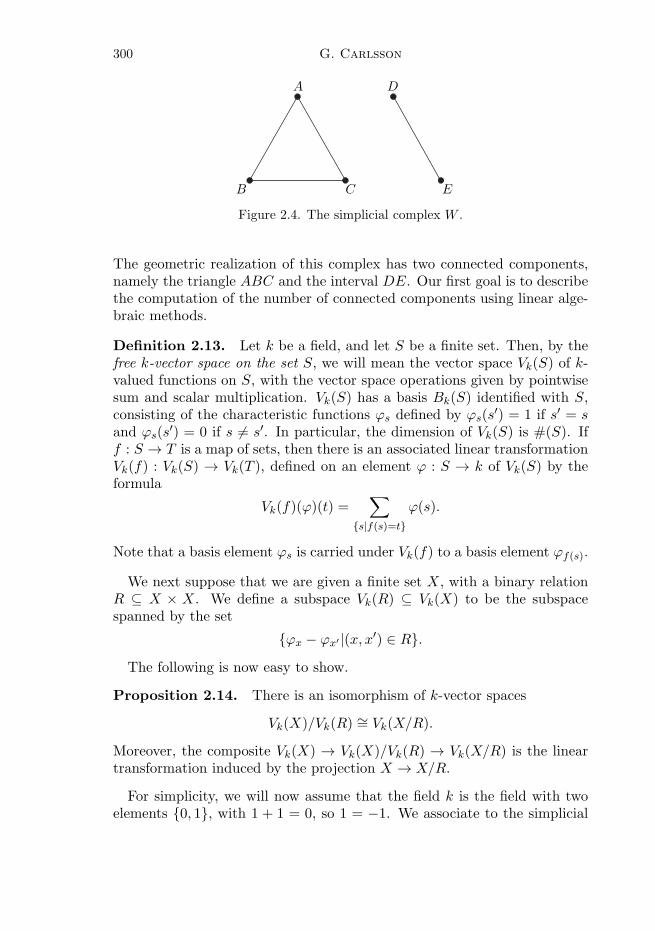
We now consider the following very simple example of an abstract sim-plicial complex, denoted by W .
The list of simplices in the corresponding simplicial complex is now
{{A}, {B}, {C}, {D}, {E}, {A,B}, {A,C}, {B,C}, {D,E}}.
300 G. Carlsson
A
B C
D
E
Figure 2.4. The simplicial complex W .
The geometric realization of this complex has two connected components,namely the triangle ABC and the interval DE. Our first goal is to describethe computation of the number of connected components using linear alge-braic methods.
Definition 2.13. Let k be a field, and let S be a finite set. Then, by thefree k-vector space on the set S, we will mean the vector space Vk(S) of k-valued functions on S, with the vector space operations given by pointwisesum and scalar multiplication. Vk(S) has a basis Bk(S) identified with S,consisting of the characteristic functions ϕs defined by ϕs(s
′) = 1 if s′ = sand ϕs(s
′) = 0 if s = s′. In particular, the dimension of Vk(S) is #(S). Iff : S → T is a map of sets, then there is an associated linear transformationVk(f) : Vk(S) → Vk(T ), defined on an element ϕ : S → k of Vk(S) by theformula
Vk(f)(ϕ)(t) =∑
{s|f(s)=t}ϕ(s).
Note that a basis element ϕs is carried under Vk(f) to a basis element ϕf(s).
We next suppose that we are given a finite set X, with a binary relationR ⊆ X × X. We define a subspace Vk(R) ⊆ Vk(X) to be the subspacespanned by the set
{ϕx − ϕx′ |(x, x′) ∈ R}.The following is now easy to show.
Proposition 2.14. There is an isomorphism of k-vector spaces
Vk(X)/Vk(R) ∼= Vk(X/R).
Moreover, the composite Vk(X) → Vk(X)/Vk(R) → Vk(X/R) is the lineartransformation induced by the projection X → X/R.
For simplicity, we will now assume that the field k is the field with twoelements {0, 1}, with 1 + 1 = 0, so 1 = −1. We associate to the simplicial
Topological pattern recognition for point cloud data 301
A B
C D
E
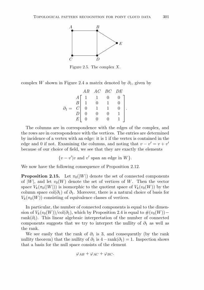
Figure 2.5. The complex X.
complex W shown in Figure 2.4 a matrix denoted by ∂1, given by
∂1 =
AB AC BC DE
A 1 1 0 0B 1 0 1 0C 0 1 1 0D 0 0 0 1E 0 0 0 1
.
The columns are in correspondence with the edges of the complex, andthe rows are in correspondence with the vertices. The entries are determinedby incidence of a vertex with an edge: it is 1 if the vertex is contained in theedge and 0 if not. Examining the columns, and noting that v − v′ = v + v′because of our choice of field, we see that they are exactly the elements
{v − v′|v and v′ span an edge in W}.We now have the following consequence of Proposition 2.12.
Proposition 2.15. Let π0(|W |) denote the set of connected componentsof |W |, and let v0(W ) denote the set of vertices of W . Then the vectorspace Vk(π0(|W |)) is isomorphic to the quotient space of Vk(v0(W )) by thecolumn space col(∂1) of ∂1. Moreover, there is a natural choice of basis forVk(π0(W )) consisting of equivalence classes of vertices.
In particular, the number of connected components is equal to the dimen-sion of Vk(v0(W ))/col(∂1), which by Proposition 2.4 is equal to #(v0(W ))−rank(∂i). This linear algebraic interpretation of the number of connectedcomponents suggests that we try to interpret the nullity of ∂1 as well asthe rank.We see easily that the rank of ∂1 is 3, and consequently (by the rank
nullity theorem) that the nullity of ∂1 is 4− rank(∂1) = 1. Inspection showsthat a basis for the null space consists of the element
ϕAB + ϕAC + ϕBC .

302 G. Carlsson
A B
C D
E
AB AC BD BE CD DE
A 1 1 0 0 0 0B 1 0 1 1 0 0C 0 1 0 0 1 0D 0 0 1 0 1 1E 0 0 0 1 0 1
Figure 2.6. A complex with a two-simplex added.
If we permit ourselves to think of the sums as unions, this linear combinationcorresponds to the union of the edges AB,AC, and BC. This union is acycle of length three in the complex W shown in Figure 2.4. It is a usefulexercise to make similar computations for other graphs, in particular n-cycles for numbers > 3, to convince ourselves that the nullity is in each casethe number of cycles in the graph, suitably interpreted. To understand theinterpretation, consider the following complex.We can see that there are two obvious cycles, AB + BD + DC + AC
and BE + ED + DB, represented by the elements of the null space ζ1 =ϕAB + ϕBD + ϕCD + ϕAC and ζ2 = ϕBE + ϕED + ϕDB. However, there isanother cycle given by
AB +BE + ED +DC + CA. (2.1)
Note, however, that the sum ζ1 + ζ2 is equal to the element
ϕAB + ϕBE + ϕED + ϕDC + ϕCA,
which is the element of the null space of ∂1 corresponding to the cycle in(2.1). The cycles actually correspond to the elements of vector space, andcan therefore be added and multiplied by scalars. This give an extremelyuseful way of organizing the cycles. In particular, one can construct a basisof the cycles, instead of counting them all individually.Next, consider the complex in Figure 2.6, with its corresponding ∂1 ma-
trix. The shading reflects the fact that there is now a two-simplex, namely{B,E,D}. As in the complex X in Figure 2.5, we have the two loopsABDC and BED. In this case, though, the loop BDE is filled in by a sim-plex, and the loop ABEDC can be deformed in the space to the loop ABDCby traversing the two-simplex. So, by analogy with the discussion of ho-motopy in Section 2.3, we should construct our formalism in such a waythat the two distinct cycles become equal. More importantly, though, weare interested in constructing vector spaces which in the end should dependonly on the underlying space, not on the particular triangulation, that is,on the particular way in which it is described as a simplicial complex.
Topological pattern recognition for point cloud data 303
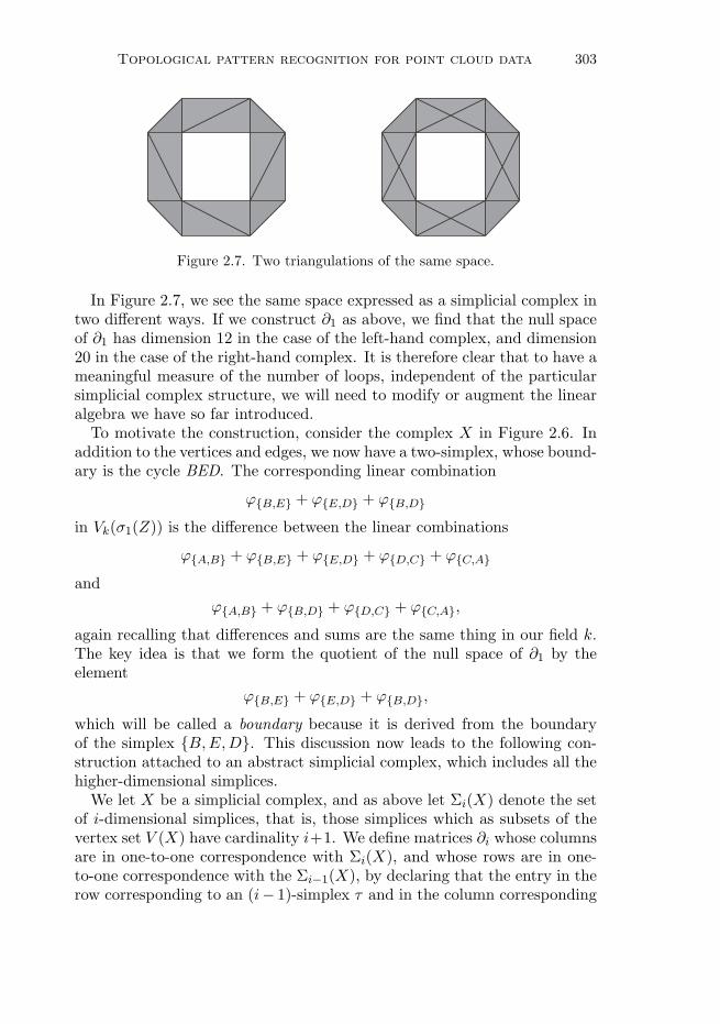
Figure 2.7. Two triangulations of the same space.
In Figure 2.7, we see the same space expressed as a simplicial complex intwo different ways. If we construct ∂1 as above, we find that the null spaceof ∂1 has dimension 12 in the case of the left-hand complex, and dimension20 in the case of the right-hand complex. It is therefore clear that to have ameaningful measure of the number of loops, independent of the particularsimplicial complex structure, we will need to modify or augment the linearalgebra we have so far introduced.To motivate the construction, consider the complex X in Figure 2.6. In
addition to the vertices and edges, we now have a two-simplex, whose bound-ary is the cycle BED. The corresponding linear combination
ϕ{B,E} + ϕ{E,D} + ϕ{B,D}in Vk(σ1(Z)) is the difference between the linear combinations
ϕ{A,B} + ϕ{B,E} + ϕ{E,D} + ϕ{D,C} + ϕ{C,A}and
ϕ{A,B} + ϕ{B,D} + ϕ{D,C} + ϕ{C,A},
again recalling that differences and sums are the same thing in our field k.The key idea is that we form the quotient of the null space of ∂1 by theelement
ϕ{B,E} + ϕ{E,D} + ϕ{B,D},
which will be called a boundary because it is derived from the boundaryof the simplex {B,E,D}. This discussion now leads to the following con-struction attached to an abstract simplicial complex, which includes all thehigher-dimensional simplices.We let X be a simplicial complex, and as above let Σi(X) denote the set
of i-dimensional simplices, that is, those simplices which as subsets of thevertex set V (X) have cardinality i+1. We define matrices ∂i whose columnsare in one-to-one correspondence with Σi(X), and whose rows are in one-to-one correspondence with the Σi−1(X), by declaring that the entry in therow corresponding to an (i− 1)-simplex τ and in the column corresponding
304 G. Carlsson
to an i-simplex τ ′ is 1 if τ ⊆ τ ′ as sets of vertices, and it is 0 otherwise.This definition is consistent with the matrices we have constructed in thespecial cases above. There is now a key observation relating the matrices ∂iand ∂i−1.
Proposition 2.16. The matrix product ∂i−1 · ∂i is equal to the zero ma-trix.
Proof. The rows of ∂i−1 ·∂i are in one-to-one correspondence with Σi−2(X),and its columns are in one-to-one correspondence with Σi(X). It is easy tosee that the entry in the row corresponding to an (i − 2)-simplex τ andin the column corresponding to an i-simplex τ ′ is equal to the number ofelements τ of Σi−1(X) which satisfy τ ⊆ τ ⊆ τ ′. This number is either 0,in the case τ ⊂ τ ′, or 2, in the case τ ⊂ τ ′. Both numbers are zero in thefield k.
The matrices ∂i can be regarded as the matrices attached to linear trans-formations from Vk(Σi(X)) to Vk(Σi−1(X), relative to the standard basesof Vk(Σi(X)). Abusing notation, we will denote the matrices and the trans-formations by ∂i. What we now have is a diagram,
· · · ∂i+2−→ Vk(Σi+1(X))∂i+1−→ Vk(Σi(X))
∂i−→ Vk(Σi−1(X))∂i−1−→ · · ·
∂2−→ Vk(Σ1(X))∂1−→ Vk(Σ0(X)),
in which each composite of two consecutive linear transformations is iden-tically zero. This observation now suggests the following definition.
Definition 2.17. By a chain complex C∗ over a field k, we will mean achoice of k-vector space Ci for every i ≥ 0, together with linear transforma-tions ∂i : Ci → Ci−1 for all i, so that ∂i−1 · ∂i ≡ 0 for all i.
We now extract information as follows. For every i, we define two subp-saces Bi and Zi of Ci. Zi is defined as the null space of ∂i, and Bi is definedas the image of ∂i+1. By Proposition 2.16, it follows that Bi ⊆ Zi, and wedefineHi(C∗) to be the quotient space Zi/Bi. One can check that in the caseof the complex in Figure 2.6, H1 turns out to be a one-dimensional vectorspace over k, with ϕAB+ϕBD+ϕDC+ϕCA as an element in Z1 whose imagein Z1/B1 is a non-trivial element, therefore a basis for H1. These vectorspaces, applied to the chain complex associated with a simplicial complex,will be called the homology groups of the complex.We now describe the linear algebra which is carried out to compute the
homology groups, and in particular their dimension. That is, we want tointerpret the computation of the homology groups of a complex in termsof row and column operations. The row and column operations will bemultiplication of a single row (column) by a non-zero element of k, addinga multiple of one row (column) to another, and transposing a pair of rows

Topological pattern recognition for point cloud data 305
(columns). We recall Remark 2.5, which asserts that given a matrix A overa field k, one may perform both row and column operations of the typedescribed above to obtain a matrix A having the normal form[
In 00 0
],
where n is the rank of A. A is uniquely determined by A.In order to study homology, we will instead need to study the normal
forms of pairs of matrices (A,B) with A ·B = 0.
Proposition 2.18. Let
UB−→ V
A−→W
be linear transformations, such that A ·B = 0. Let F : U → U , G : V → V ,and H : W → W be invertible linear transformations. Then we haveHAG−1 ·GBF = 0, and there is an isomorphism of vector spaces
N(A)/im(B) ∼= N(HAG−1)/im(GBF ).
Proof. Entirely analogous to Proposition 2.3.
The matrix version now uses the following set of admissible operations onsuch a pair. They will be the following.
(1) An arbitrary row operation on A.
(2) An arbitrary column operation on B.
(3) Perform a column operation on A and a row operation on B simultane-ously, with the operations related as follows. If the column operationon A is multiplication of the ith column by a non-zero constant x, thenthe row operation on B is multiplication of the ith row by x−1. If thecolumn operation on A is the transposition of two columns, then therow operation on B is the transposition of the corresponding rows ofB. Finally, if the column operation on A is the addition of x timesthe ith column to the jth column, then the row operation on B is thesubtraction of x times the jth row from the ith row.
Note that if we apply any of these operations to a pair (A,B) to obtaina pair (A′, B′), then (A′, B′) also satisfies A′ · B′ = 0. We now have thefollowing counterpart of Proposition 2.4 above.
Proposition 2.19. Given a pair (A,B), with A · B = 0, we can performoperations of the type described above to obtain a pair (A′, B′), with
In 0 00 0 00 0 0
,
0 0 00 0 00 0 Im
.
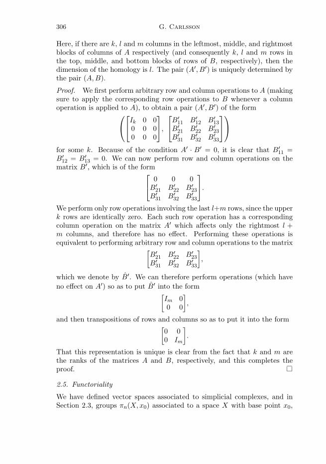
306 G. Carlsson
Here, if there are k, l and m columns in the leftmost, middle, and rightmostblocks of columns of A respectively (and consequently k, l and m rows inthe top, middle, and bottom blocks of rows of B, respectively), then thedimension of the homology is l. The pair (A′, B′) is uniquely determined bythe pair (A,B).
Proof. We first perform arbitrary row and column operations to A (makingsure to apply the corresponding row operations to B whenever a columnoperation is applied to A), to obtain a pair (A′, B′) of the form
Ik 0 00 0 00 0 0
,
B
′11 B′
12 B′13
B′21 B′
22 B′23
B′31 B′
32 B′33
for some k. Because of the condition A′ · B′ = 0, it is clear that B′11 =
B′12 = B′
13 = 0. We can now perform row and column operations on thematrix B′, which is of the form
0 0 0B′
21 B′22 B′
23
B′31 B′
32 B′33
.
We perform only row operations involving the last l+m rows, since the upperk rows are identically zero. Each such row operation has a correspondingcolumn operation on the matrix A′ which affects only the rightmost l +m columns, and therefore has no effect. Performing these operations isequivalent to performing arbitrary row and column operations to the matrix[
B′21 B′
22 B′23
B′31 B′
32 B′33
],
which we denote by B′. We can therefore perform operations (which have
no effect on A′) so as to put B′ into the form[Im 00 0
],
and then transpositions of rows and columns so as to put it into the form[0 00 Im
].
That this representation is unique is clear from the fact that k and m arethe ranks of the matrices A and B, respectively, and this completes theproof.
2.5. Functoriality
We have defined vector spaces associated to simplicial complexes, and inSection 2.3, groups πn(X,x0) associated to a space X with base point x0,
Topological pattern recognition for point cloud data 307
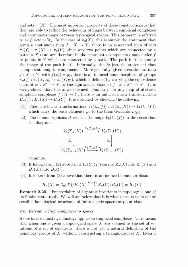
and sets π0(X). The most important property of these constructions is thatthey are able to reflect the behaviour of maps between simplicial complexesand continuous maps between topological spaces. This property is referredto as functoriality. In the case of π0(X), this is simply the statement thatgiven a continuous map f : X → Y , there is an associated map of setsπ0(f) : π0(X) → π0(Y ), since any two points which are connected by apath in X (and are therefore in the same path component) map under fto points in Y which are connected by a path. The path in Y is simplythe image of the path in X. Informally, this is just the statement that‘components map to components’. More generally, given a continuous mapf : X → Y , with f(x0) = y0, there is an induced homomorphism of groupsπn(f) : πn(X,x0)→ πn(Y, y0), which is defined by carrying the equivalenceclass of ϕ : Sn → Y to the equivalence class of f · ϕ : Sn → Y . It iseasily shown that this is well defined. Similarly, for any map of abstractsimplicial complexes f : X → Y , there is an induced linear transformationHn(f) : Hn(X)→ Hn(Y ). It is obtained by showing the following.
(1) There are linear transformations Vk(Σn(f)) : Vk(Σn(X))→ Vk(Σn(Y ))which carry the basis elements ϕτ to the basis elements ϕf(τ).
(2) The homomorphisms ∂i respect the maps Vk(Σn(f)) in the sense thatthe diagrams
Vk(Σn(X)) Vk(Σn(Y ))
Vk(Σn−1(X)) Vk(Σn−1(Y ))�
∂n
�Vk(Σn(f))
�∂n
�Vk(Σn(f))
commute.
(3) It follows from (2) above that Vn(Σn(f)) carries Zn(X) into Zn(Y ) andBn(X) into Bn(Y ).
(4) It follows from (3) above that there is an induced homomorphism
Hn(X) = Zn(X)/Bn(X)Hn(f)−→ Zn(Y )/Bn(Y ) = Hn(Y ).
Remark 2.20. Functoriality of algebraic invariants in topology is one ofits fundamental tools. We will see below that it is what permits us to definesensible homological invariants of finite metric spaces or point clouds.
2.6. Extending from complexes to spaces
As we have defined it, homology applies to simplicial complexes. This meansthat when one is given a topological space X, say defined as the set of so-lutions of a set of equations, there is not yet a natural definition of thehomology groups of X, without constructing a triangulation of X. Even if
308 G. Carlsson
one can construct a triangulation, it is not clear why a different triangula-tion would not give a different answer. The problem of extending homologyspaces without a given triangulation was studied intensively in the early1900s, and was resolved by Eilenberg (1944). He defined homology groupsHn(X) (called the singular homology groups) for any space X by construct-ing a chain complex of infinite-dimensional vector spaces (a basis of Cn(X)is given by the set of all continuous maps ∆n → X) whose homology agreeswith the simplicially constructed homology for any triangulation of X. Thehomology groups constructed with these complexes are functorial for anycontinuous map f : X → Y , by which we mean that there is a lineartransformation Hn(f) : Hn(X) → Hn(Y ) associated to f . An additionalimportant property is homotopy invariance, which asserts that if two mapsf, g : X → Y are homotopic (see Definition 2.6), then the linear transforma-tions Hn(f) and Hn(g) are equal. This is a powerful property, and it allowsdirect calculations of homology in some cases. We say that a topologicalspace X is contractible if idX is homotopic to a constant map.
Example 2.21. Rn is contractible, because we have the explicit homotopyH(v, t) = (1− t)v from idRn to the constant map with value 0.
Proposition 2.22. If X is a contractible space, then Hn(X) = {0} for alln > 0.
Proof. By the homotopy property and functoriality, the identity transfor-mation on Hn(X) is equal to the composite Hn(X) → Hn(x0) → Hn(X),where x0 ∈ X is a point such that f is homotopic to the constant map withvalue x0. But it is easy to check directly that Hn(x0) = {0}, and it nowfollows that every element in Hn(X) is 0.
Remark 2.23. The singular homology groups are of course impossibleto compute directly, since in particular they involve linear algebra on vec-tor spaces of uncountable dimension. This means that when we wish tocompute homology, we must either construct a triangulation or use othercomputational techniques, called excision and long exact sequences, whichhave been developed for this purpose. The important point in the definitionis that it gives well-defined groups for any space, which behave functoriallyfor continuous maps.
2.7. Making homology more sensitive
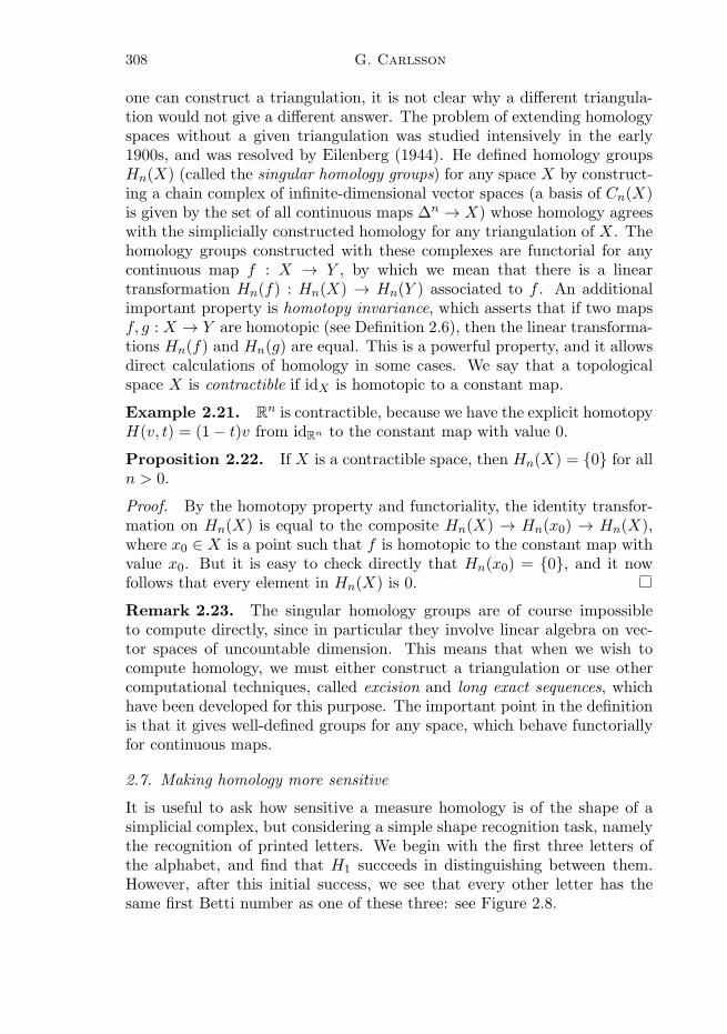
It is useful to ask how sensitive a measure homology is of the shape of asimplicial complex, but considering a simple shape recognition task, namelythe recognition of printed letters. We begin with the first three letters ofthe alphabet, and find that H1 succeeds in distinguishing between them.However, after this initial success, we see that every other letter has thesame first Betti number as one of these three: see Figure 2.8.
Topological pattern recognition for point cloud data 309
A(a) β1 = 1
B(b) β1 = 2
C(c) β1 = 0
β1 = 0 {C,E,F,G,H, I, J,K,L,M,N, S,T,U,V,W,X,Y,Z}β1 = 1 {A,D,O,P,Q,R}β1 = 2 {B}
Figure 2.8. Discrimination of letters by first Betti number.
Homology can be refined to discriminate more finely between the letters.To understand how this works, we digress a bit to discuss how an analo-gous problem in manifold topology is approached. In Section 2.6, we sawthat the homology groups Hi(R
n) vanish for all i > 0. What this means isthat homology is unable to distinguish between Rm and Rn when m = n.From the point of view of a topologist who is interested in distinguishingdifferent manifolds from each other, this means that homology is in someways a relatively weak invariant. This failure can be addressed by comput-ing homology on ‘auxiliary’ or ‘derived’ spaces, constructed using variousgeometric constructions.
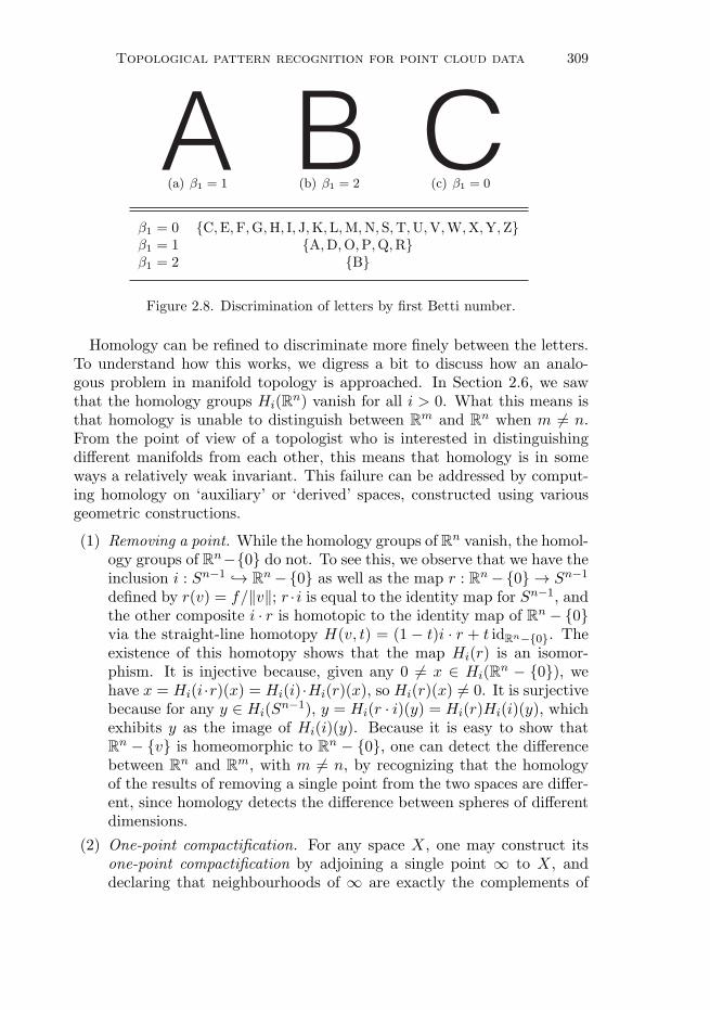
(1) Removing a point. While the homology groups of Rn vanish, the homol-ogy groups of Rn−{0} do not. To see this, we observe that we have theinclusion i : Sn−1 ↪→ Rn−{0} as well as the map r : Rn−{0} → Sn−1
defined by r(v) = f/‖v‖; r ·i is equal to the identity map for Sn−1, andthe other composite i · r is homotopic to the identity map of Rn − {0}via the straight-line homotopy H(v, t) = (1 − t)i · r + t idRn−{0}. Theexistence of this homotopy shows that the map Hi(r) is an isomor-phism. It is injective because, given any 0 = x ∈ Hi(R
n − {0}), wehave x = Hi(i ·r)(x) = Hi(i) ·Hi(r)(x), so Hi(r)(x) = 0. It is surjectivebecause for any y ∈ Hi(S
n−1), y = Hi(r · i)(y) = Hi(r)Hi(i)(y), whichexhibits y as the image of Hi(i)(y). Because it is easy to show thatRn − {v} is homeomorphic to Rn − {0}, one can detect the differencebetween Rn and Rm, with m = n, by recognizing that the homologyof the results of removing a single point from the two spaces are differ-ent, since homology detects the difference between spheres of differentdimensions.
(2) One-point compactification. For any space X, one may construct itsone-point compactification by adjoining a single point ∞ to X, anddeclaring that neighbourhoods of ∞ are exactly the complements of

310 G. Carlsson
∞
0
Figure 2.9. One-point compactification.
A
Figure 2.10. Removing singular points.
compact subsets of X together with∞. Figure 2.9 shows the one-pointcompactification of the real line. Note that although the real line iscontractible and therefore has vanishing homology, its one-point com-pactification is homeomorphic to the circle, and has non-vanishing H1.
(3) Removing singular points. Consider the space given by the crossingof two lines. This space is also contractible, as one can easily see byretracting each line segment onto the crossing point A. On the otherhand, we recognize that its shape has features which distinguish it froman interval or a circle, and might want to detect that homologically. Ifwe remove the singular point A, we will find that the space remainingbreaks up into four distinct components, which can be detected by H0.
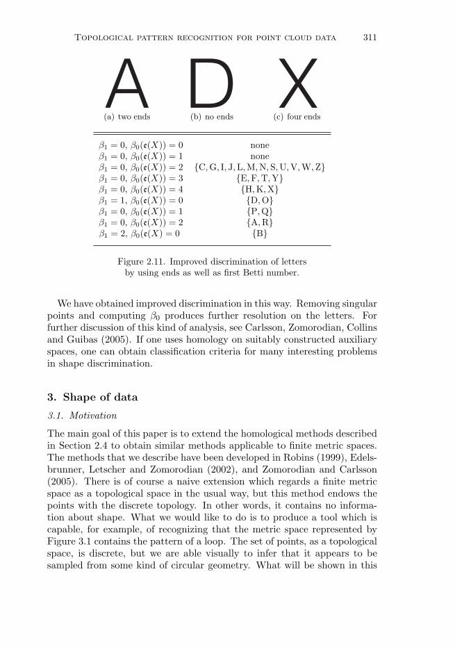
To think through how we might apply these ideas to the problem ofdistinguishing between letters, let us define an end of a spaceX to be a pointx ∈ X, so that there is a neighbourhood N of x which is homeomorphic to[0, 1), and so that the homeomorphism carries x to 0.In this case, the auxiliary or derived space is the set of ends of the space,
e(X), and we can compute its zero-dimensional homology H0, to get theBetti number β0. We now obtain the partition of the set of letters shownin Figure 2.11.
Topological pattern recognition for point cloud data 311
A(a) two ends
D(b) no ends
X(c) four ends
β1 = 0, β0(e(X)) = 0 noneβ1 = 0, β0(e(X)) = 1 noneβ1 = 0, β0(e(X)) = 2 {C,G, I, J,L,M,N, S,U,V,W,Z}β1 = 0, β0(e(X)) = 3 {E,F,T,Y}β1 = 0, β0(e(X)) = 4 {H,K,X}β1 = 1, β0(e(X)) = 0 {D,O}β1 = 0, β0(e(X)) = 1 {P,Q}β1 = 0, β0(e(X)) = 2 {A,R}β1 = 2, β0(e(X) = 0 {B}
Figure 2.11. Improved discrimination of lettersby using ends as well as first Betti number.
We have obtained improved discrimination in this way. Removing singularpoints and computing β0 produces further resolution on the letters. Forfurther discussion of this kind of analysis, see Carlsson, Zomorodian, Collinsand Guibas (2005). If one uses homology on suitably constructed auxiliaryspaces, one can obtain classification criteria for many interesting problemsin shape discrimination.
3. Shape of data
3.1. Motivation
The main goal of this paper is to extend the homological methods describedin Section 2.4 to obtain similar methods applicable to finite metric spaces.The methods that we describe have been developed in Robins (1999), Edels-brunner, Letscher and Zomorodian (2002), and Zomorodian and Carlsson(2005). There is of course a naive extension which regards a finite metricspace as a topological space in the usual way, but this method endows thepoints with the discrete topology. In other words, it contains no informa-tion about shape. What we would like to do is to produce a tool which iscapable, for example, of recognizing that the metric space represented byFigure 3.1 contains the pattern of a loop. The set of points, as a topologicalspace, is discrete, but we are able visually to infer that it appears to besampled from some kind of circular geometry. What will be shown in this

312 G. Carlsson
Figure 3.1. A ‘statistical circle’.
section is that it is possible to develop just such a tool. To motivate thisconstruction, we will look at a commonly used statistical methodology.
3.2. Single linkage clustering
The very simplest aspect of the shape of a geometric object is its number ofconnected components. Statisticians have thought a great deal about whatthe counterpart to connected components should be for point cloud data,under the heading of clustering: see Hartigan (1975) and Kogan (2007). Onescheme for clustering proceeds as follows. We suppose we are given a finitemetric space with points X = {x1, . . . , xn}, and given pairwise distances.For every non-negative threshold R, we may form the relation ∼R on theset X by the criterion
x ∼R x′ if and only if d(x, x′) ≤ R.
We let �R denote the equivalence relation generated by ∼R. The set ofequivalence classes under �R now gives a partition of X, which can bethought of as a candidate for the connected components in X. So for eachthreshold R, we obtain a partition of X. One can now ask which choice ofR is the ‘right’ one. This is an ill-defined question, although there are inter-esting heuristics. Another approach is to observe that there is compatibilityacross changes in R, in that if R ≤ R′, then the partition associated to R′ iscoarser than the partition associated to R, as is indicated in Figure 3.2. Thediagram indicates the change in clustering as the threshold is altered, andshows the increasing coarseness as R increases. What was recognized bystatisticians is that there is a single profile, called a dendrogram, which en-codes the clusterings at all the thresholds simultaneously. Figure 3.3 showsa dendrogram which is associated to the situation given above. The resultis a tree (a simplicial complex with no loops) T together with a referencemap from T to the non-negative real line. This tree can be viewed all atonce. The clustering at a given threshold R is given by drawing a horizontal

Topological pattern recognition for point cloud data 313
Figure 3.2. Single linkage hierarchical clustering.
Figure 3.3. Dendrogram.
line at level R across the tree, and the clusters correspond to the points ofintersection. In Figure 3.3, the reference map is the height function abovethe x-axis.There is another way to interpret the dendrogram, less visually but for-
mally identical. For each threshold R, we will let XR denote the set ofequivalence classes for the equivalence relation �R. Because the partitiononly coarsens as R increases, there is a map of sets XR → XR′ wheneverR ≤ R′, which assigns to each cluster at level R the (unique) cluster at levelR′ in which it is included. This construction is sufficiently useful that wewill give it a name.
Definition 3.1. By a persistent set, we will mean a family of sets {XR}R∈Rtogether with set maps
ϕR′R : XR → XR′ for all R ≤ R′,
so that
ϕR′′R′ ϕR′
R = ϕR′′R for all R ≤ R′ ≤ R′′.
More generally, for any kind of objects, such as simplicial complexes, vectorspaces or topological spaces, we may speak of a persistent object as a familyof such objects parametrized by R, together with maps (maps of simplicial

314 G. Carlsson
complexes, linear transformations, continuous maps, etc.) from the objectparametrized by r to the one parametrized by r′ whenever r ≤ r′, with thesame compatibilities mentioned above.
For each persistent set there is an associated dendrogram and vice versa.There is a reformulation of the dendrogram (and hence a persistent set) as-sociated to a finite metric space using topological notions which will greatlyclarify the development of methods of defining higher-dimensional homologyfor finite metric spaces.
Definition 3.2. Given any finite metric space X and non-negative realnumber R, we construct an abstract simplicial complex VR(X,R), calledthe Vietoris–Rips complex of X, by letting its vertex set be the underlyingset of X, and declaring that any subset {x0, . . . , xn} of X is a simplex ofVR(X,R) if and only if
d(xi, xj) ≤ R for all i, j ∈ {0, . . . , n}.We note that whenever R ≤ R′ there is an inclusion VR(X,R) ↪→VR(X,R′),because the vertex sets of the two abstract complexes are the same, and thatany simplex of VR(X,R) is also a simplex of V (X,R′). It follows that weobtain maps
|VR(X,R)| → |VR(X,R′)|as well. In short, the family of Vietoris–Rips complexes {VR(X,R)}R∈Rforms a persistent simplicial complex.
The point of this definition is that given any finite metric space X, wemay define the set π0(|VR(X,R)|) of connected components of |VR(X,R)|,and due to the functoriality of the construction π0, we obtain a persistentset {π0(|VR(X,R)|)}R. This persistent set can easily be seen to be identicalto the persistent set obtained above. The point is that it is induced by amap of topological spaces, which will point the way to defining homologicalshape invariants of finite metric spaces.
3.3. Persistence
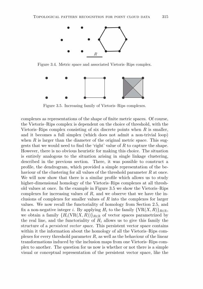
The value of the Vietoris–Rips construction is that for each threshold weare able to construct a simplicial complex and therefore a topological space,rather than just a partitioning or clustering of the finite metric space. Inthe example shown in Figure 3.4 the underlying metric space consists of sixpoints, and is pictured on the left. The lower bar is the threshold param-eter R, and on the right we have a picture of the Vietoris–Rips complexassociated to this metric space and this threshold. The metric space looksas if it might be sampled from a loop, and we note that the Vietoris–Ripscomplex contains a loop. This suggests that we should use Vietoris–Rips
Topological pattern recognition for point cloud data 315
R
Figure 3.4. Metric space and associated Vietoris–Rips complex.
Figure 3.5. Increasing family of Vietoris–Rips complexes.
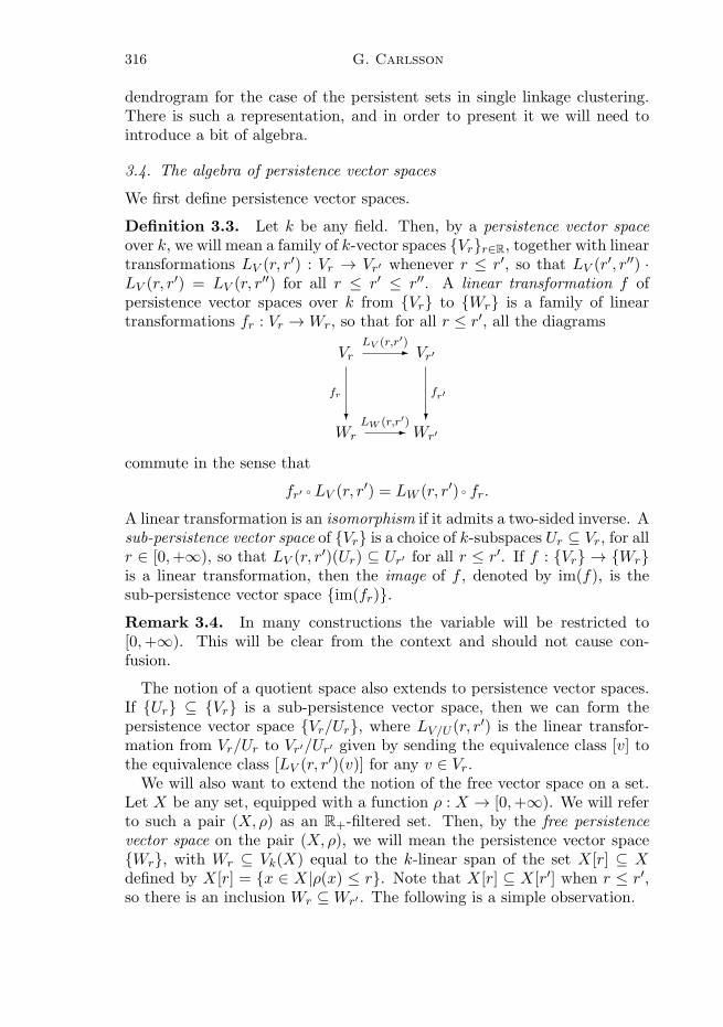
complexes as representations of the shape of finite metric spaces. Of course,the Vietoris–Rips complex is dependent on the choice of threshold, with theVietoris–Rips complex consisting of six discrete points when R is smaller,and it becomes a full simplex (which does not admit a non-trivial loop)when R is larger than the diameter of the original metric space. This sug-gests that we would need to find the ‘right’ value of R to capture the shape.However, there is no obvious heuristic for making this choice. The situationis entirely analogous to the situation arising in single linkage clustering,described in the previous section. There, it was possible to construct aprofile, the dendrogram, which provided a simple representation of the be-haviour of the clustering for all values of the threshold parameter R at once.We will now show that there is a similar profile which allows us to studyhigher-dimensional homology of the Vietoris–Rips complexes at all thresh-old values at once. In the example in Figure 3.5 we show the Vietoris–Ripscomplexes for increasing values of R, and we observe that we have the in-clusions of complexes for smaller values of R into the complexes for largervalues. We now recall the functoriality of homology from Section 2.5, andfix a non-negative integer i. By applying Hi to the family {VR(X,R)}R∈R,we obtain a family {Hi(VR(X,R))}R∈R of vector spaces parametrized bythe real line, and the functoriality of Hi allows us to give this family thestructure of a persistent vector space. This persistent vector space containswithin it the information about the homology of all the Vietoris–Rips com-plexes for every threshold parameter R, as well as the behaviour of the lineartransformations induced by the inclusion maps from one Vietoris–Rips com-plex to another. The question for us now is whether or not there is a simplevisual or conceptual representation of the persistent vector space, like the
316 G. Carlsson
dendrogram for the case of the persistent sets in single linkage clustering.There is such a representation, and in order to present it we will need tointroduce a bit of algebra.
3.4. The algebra of persistence vector spaces
We first define persistence vector spaces.
Definition 3.3. Let k be any field. Then, by a persistence vector spaceover k, we will mean a family of k-vector spaces {Vr}r∈R, together with lineartransformations LV (r, r
′) : Vr → Vr′ whenever r ≤ r′, so that LV (r′, r′′) ·
LV (r, r′) = LV (r, r
′′) for all r ≤ r′ ≤ r′′. A linear transformation f ofpersistence vector spaces over k from {Vr} to {Wr} is a family of lineartransformations fr : Vr →Wr, so that for all r ≤ r′, all the diagrams
Vr Vr′
Wr Wr′�
fr
�LV (r,r′)
�
fr′
�LW (r,r′)
commute in the sense that
fr′ ◦ LV (r, r′) = LW (r, r′) ◦ fr.
A linear transformation is an isomorphism if it admits a two-sided inverse. Asub-persistence vector space of {Vr} is a choice of k-subspaces Ur ⊆ Vr, for allr ∈ [0,+∞), so that LV (r, r
′)(Ur) ⊆ Ur′ for all r ≤ r′. If f : {Vr} → {Wr}is a linear transformation, then the image of f , denoted by im(f), is thesub-persistence vector space {im(fr)}.Remark 3.4. In many constructions the variable will be restricted to[0,+∞). This will be clear from the context and should not cause con-fusion.
The notion of a quotient space also extends to persistence vector spaces.If {Ur} ⊆ {Vr} is a sub-persistence vector space, then we can form thepersistence vector space {Vr/Ur}, where LV/U (r, r
′) is the linear transfor-mation from Vr/Ur to Vr′/Ur′ given by sending the equivalence class [v] tothe equivalence class [LV (r, r
′)(v)] for any v ∈ Vr.We will also want to extend the notion of the free vector space on a set.
Let X be any set, equipped with a function ρ : X → [0,+∞). We will referto such a pair (X, ρ) as an R+-filtered set. Then, by the free persistencevector space on the pair (X, ρ), we will mean the persistence vector space{Wr}, with Wr ⊆ Vk(X) equal to the k-linear span of the set X[r] ⊆ Xdefined by X[r] = {x ∈ X|ρ(x) ≤ r}. Note that X[r] ⊆ X[r′] when r ≤ r′,so there is an inclusion Wr ⊆Wr′ . The following is a simple observation.

Topological pattern recognition for point cloud data 317
Proposition 3.5. A linear combination∑
x axx ∈ Vk(X) lies in Wr if andonly if ax = 0 for all x with ρ(x) > r.
We will write {Vk(X, ρ)r} for this persistence vector space. We say apersistence vector space is free if it is isomorphic to one of the form Vk(X, ρ)for some (X, ρ), and we say it is finitely generated if X can be taken to befinite.
Definition 3.6. A persistence vector space is finitely presented if it isisomorphic to a persistence vector space of the form {Wr}/ im(f) for somelinear transformation f : {Vr} → {Wr} between finitely generated freepersistence vector spaces {Vr} and {Wr}.
The choice of a basis for vector spaces V and W allows us to representlinear transformations from V to W by matrices. We will now show thatthere is a similar representation for linear transformations between free per-sistence vector spaces. For any pair (X,Y ) of finite sets and field k, an(X,Y )-matrix is an array [axy] of elements of axy of k. We write r(x) forthe row corresponding to x ∈ X, and c(y) for the column corresponding to y.For any finitely generated free persistence vector space {Vr} = {Vk(X, ρ)r},we observe that Vk(X, ρ)r = Vk(X) for r sufficiently large, since X is finite.Therefore, for any linear transformation f : {Vk(Y, σ)r} → {Vk(X, ρ)r} offinitely generated free persistence vector spaces, f gives a linear transfor-mation f∞ : Vk(Y )→ Vk(X) between finite-dimensional vector spaces overk, and using the bases {ϕx}x∈X of Vk(X) and {ϕy}y∈Y of Vk(Y ) determinesan (X,Y )-matrix A(f) = [axy] with entries in k. Note that in order toobtain the usual notion of a matrix as a rectangular array, we would needto impose total orderings on X and Y , but the matrix manipulations do notrequire this.
Proposition 3.7. The (X,Y )-matrix A(f) has the property that axy = 0whenever ρ(x) > σ(y). Any (X,Y )-matrix A satisfying these conditionsuniquely determines a linear transformation of persistence vector spaces
fA : {Vk(Y, σ)r} → {Vk(X, ρ)r}and the correspondences f → A(f) and A→ fA are inverses to each other.
Proof. The basis vector y lies in Vk(Y, σ)σ(y). On the other hand,
f(ϕy) =∑x∈X
axyϕx.
By Proposition 3.5, on the other hand,∑
x∈X axyϕx only lies in Vk(X, ρ)σ(y)if all coefficients axy, for ρ(x) > σ(y), are zero.
318 G. Carlsson
When we are given a pair of R+-filtered finite sets (X, ρ) and (Y, σ),we will call an (X,Y )-matrix satisfying the conditions of Proposition 3.7(ρ, σ)-adapted.Suppose now that we are given (X, ρ) and (Y, σ), with ρ and σ both
[0,+∞)-valued functions on X and Y , respectively. Then any matrix A =[axy] satisfying the conditions of Proposition 3.7 determines a persistencevector space via the correspondence
Aθ−→ Vk(X, ρ)/im(fA).
We have the following facts about this construction.
Proposition 3.8. For any A as described above, θ(A) is a finitely pre-sented persistence vector space. Moreover, any finitely presented persistencevector space is isomorphic to one of the form θ(A) for some such matrix A.
Proof. Immediate from the correspondence between matrices and lineartransformations given in Proposition 3.7.
Proposition 3.9. Let (X, ρ) be an R+-filtered set. Then, under the ma-trix/linear transformation correspondence, the automorphisms of Vk(X, ρ)are identified with the group of all invertible (ρ, ρ)-adapted (X,X)-matrices.
We now have the following sufficient criterion for θ(A) to be equal toθ(A′), entirely analogous to Proposition 2.4.
Proposition 3.10. Let (X, ρ) and (Y, σ) be R+ filtered sets, and let A bea (ρ, σ)-adapted (X,Y )-matrix. Let B and C be (ρ, ρ)-adapted (respectively(σ, σ)-adapted) (X,X)-matrices (respectively (Y, Y )-matrices). Then BACis also (ρ, σ)-adapted, and the persistence vector space θ(A) is isomorphicto θ(BAC).
Remark 3.11. For any r ∈ F , where F is a field, the elementary matrixe(i, j, r) is given by ett(i, j, r) = 1 for all t, eij(i, j, r) = r, and euv(i, j, t) = 0whenever (u, v) = (i, j) and u = v. Left multiplication by e(i, j, r) has theeffect of adding r times the jth row to the ith row, and right multiplicationby e(i, j, r) has the effect of adding r times the ith column to the jth column.This observation now suggests that given two R+ filtered sets (X, ρ) and(Y, σ), and a (ρ, σ)-adapted matrix A, we define an adapted row operation tobe an operation which adds a multiple of r(x) to r(x′), where ρ(x) ≥ ρ(x′).Similarly, we define an adapted column operation to be an operation whichadds a multiple of c(y) to c(y′), where σ(y) ≤ σ(y′).
We will use this result to classify up to isomorphism all finitely presentedpersistence vector spaces. We begin by defining a persistence vector spaceP (a, b) for every pair (a, b), where a ∈ R+, b ∈ R+∪{+∞}, and a < b, withthe obvious interpretation when b = +∞. P (a, b) is defined by P (a, b)r = k

Topological pattern recognition for point cloud data 319
for r ∈ [a, b), P (a, b) = {0} when r /∈ [a, b), and where L(r, r′) = idkwhenever r, r′ ∈ [a, b). This definition can be interpreted in the obviousway when b = +∞. We note that P (a, b) is finitely presented. For, in thecase where b is finite, let (X, ρ) and (Y, σ) denote R+-filtered sets (X, ρ)and (Y, σ), with the underlying sets consisting of single elements x and y,and with ρ(x) = a and σ(y) = b. Then the (1 × 1) (X,Y )-matrix matrix[1] is (ρ, σ)-adapted since a ≤ b, and it is clear that P (a, b) is isomorphicto θ([1]). When b = +∞, P (a, b) is isomorphic to the persistence vectorspace Vk(X, ρ), and can therefore be written as θ(0), where 0 denotes thezero linear transformation from the persistence vector space {0}.Proposition 3.12. Every finitely presented persistence vector space overk is isomorphic to a finite direct sum of the form
P (a1, b1)⊕ P (a2, b2)⊕ · · · ⊕ P (an, bn) (3.1)
for some choices ai ∈ [0,+∞), bi ∈ [0,+∞], and ai < bi for all i.
Proof. It is clear that a (ρ, σ)-adapted (X,Y )-matrix A which has theproperty that every row and column has at most one non-zero element,which is equal to 1, has the property that θ(A) is of the form described inthe proposition. For if we let {(x1, y1), (x2, y2), . . . , (xn, yn)} be all the pairs(xi, yi) so that axi,yi = 1, then there is a decomposition
θ(A) ∼=⊕i
P (ρ(xi), σ(yi))⊕⊕
x∈X−{x1,...,xn}P (ρ(x),+∞).
So, it suffices to construct matrices B and C, which are (ρ, ρ)-adapted (re-spectively (σ, σ)-adapted) (X,X)-matrices (respectively (Y, Y )-matrices),so that BAC has the property that every row and column has at mostone non-zero element, and that element is 1. To see that we can do this, weadapt the row and column operation approach to this setting. The (ρ, σ)-adapted row and column operations consist of all possible multiplicationsof a row or column by a non-zero element of k, all possible additions of amultiple of r(x) to r(x′) when ρ(x) ≥ ρ(x′), and all possible additions of amultiple of c(y) to c(y′) when σ(y) ≤ σ(y′). We claim that by performing(ρ, σ)-adapted row and column operations we can arrive at a matrix withat most one non-zero entry in each row and column. To see this, first finda y which maximizes σ(y) over the set of all y with c(y) = 0. Next, find anx which minimizes ρ(x) over the set of all x for which the entry axy = 0.Because of the way x is chosen, we are free to add multiples of r(x) to allthe other rows so as to ‘zero out’ c(y) except in the xy-entry. Because of theway y is chosen, we can add multiples of c(y) to zero out r(x) except in thexy-slot, without affecting c(y). The result is a matrix in which the uniquenon-zero element in both r(x) and c(y) is axy. By multiplying r(x) by 1/axy,we can make the xy-entry in the transformed matrix = 1. By deleting r(x)
320 G. Carlsson
and c(y), we obtain a (X − {x}, Y − {y})-matrix which is (ρ′, σ′)-adapted,where ρ′ and σ′ are the restrictions of ρ and σ to X − {x} and Y − {y},respectively. We can now apply the process inductively to this matrix. Eachof the row and column operations required can be interpreted as row andcolumns on the original matrix, and will have no effect on r(x) or c(y).The result is that by iterating this procedure, we will eventually arrive ata matrix with only zero entries, and it is clear that the transformed matrixhas at most one non-zero element in each row and column. The result nowfollows by Proposition 3.10.
We will also establish that any two decompositions of the form (3.1) abovefor a given persistence vector space are essentially unique.
Proposition 3.13. Suppose that {Vr} is a finitely presented persistencevector space over k, and that we have two decompositions
{Vr} ∼=⊕i∈I
P (ai, bi) and {Vr} ∼=⊕j∈J
P (cj , dj),
where I and J are finite sets. Then #(I) = #(J), and the set of pairs(ai, bi) occurring, with multiplicities, is identical to the set of pairs (cj , dj)occurring.
Proof. We let amin and cmin denote the smallest value of ai and cj , re-spectively; amin can be characterized intrinsically as min{r|Vr = 0}, andit follows that amin = cmin. Next, let bmin denote min{bi|ai = amin}, andmake the corresponding definition for dmin; bmin is also defined intrinsicallyas min{r′|N(L(r, r′)) = 0}, where N denotes null space, so bmin = dmin aswell. This means that P (amin, bmin) appears in both decompositions. Foreach decomposition, we consider the sum of all the occurrences of the sum-mand P (amin, bmin). They are both sub-persistence vector spaces of {Vr},and can in fact be characterized intrinsically as the sub-persistence vectorspace {Wr}, where Wr is the null space of the linear transformation
im(L(amin, r))L(r,bmin)|im(L(amin,r))−−−−−−−−−−−−−−→ Vbmin
.
It now follows that the number of summands of the form P (amin, bmin) inthe two decompositions are the same, and further that they correspondisomorphically under the decompositions. Let I ′ denote the subset of Iobtained by removing all i so that ai = amin and bi = bmin, and defineJ ′ correspondingly. We can now form the quotient of {Vr} by {Wr}, andobserve that we obtain identifications
{Vr}/{Wr} ∼=⊕i∈I′
P (ai, bi) and {Vr}/{Wr} ∼=⊕j∈J ′
P (cj , dj).

Topological pattern recognition for point cloud data 321
(a) barcode (b) persistence diagram
Figure 3.6. Two methods for representing persistent vector spaces.
By an induction on the number of summands in the decompositions, weobtain the result.
We observe that there is an algorithm analogous to the one constructedin Proposition 2.19 for computing the homology, in this case using adaptedrow and column operations in place of arbitrary operations. This algorithmthen produces a presentation for persistent homology.The isomorphism classes of finitely presented persistence vector spaces
are in one-to-one correspondence with finite subsets (with multiplicity) ofthe set {(a, b)|a ∈ [0,+∞), b ∈ [0,+∞], and a < b}. Such sets can berepresented visually in two distinct ways, one as families of intervals on thenon-negative real lines, and the other as a collection of points in the subset{(x, y)|x ≥ 0 and y > x} of the first quadrant in the (x, y)-plane. In thesecond case, one must place points with b = +∞ above the whole diagramin a horizontal line indicating infinity. The first representation is called abarcode, and the second a persistence diagram. We will use and refer tothese representations interchangeably.We now have a solution to the problem posed in Section 3.1. We may asso-
ciate to any finite metric space a persistence barcode or persistence diagram.What has now happened is that the Betti numbers have been replaced bythe barcodes. The way to reconcile these two notions is that, roughly speak-ing, the persistence barcodes often consist of some ‘short’ intervals and some‘long’ intervals. The short intervals are typically considered noisy, and thelong ones are considered to correspond to larger-scale geometric features,which one would expect to have a correspondence with the features of aspace from which the metric space is sampled.Figure 3.7 shows the persistence barcode and persistence diagram for
one-dimensional homology associated to the sampled version of a circle.
322 G. Carlsson
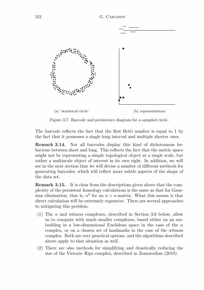
(a) ‘statistical circle’ (b) representations
Figure 3.7. Barcode and persistence diagram for a sampled circle.
The barcode reflects the fact that the first Betti number is equal to 1 bythe fact that it possesses a single long interval and multiple shorter ones.
Remark 3.14. Not all barcodes display this kind of dichotomous be-haviour between short and long. This reflects the fact that the metric spacemight not be representing a simple topological object at a single scale, butrather a multiscale object of interest in its own right. In addition, we willsee in the next section that we will devise a number of different methods forgenerating barcodes, which will reflect more subtle aspects of the shape ofthe data set.
Remark 3.15. It is clear from the descriptions given above that the com-plexity of the persistent homology calculations is the same as that for Gaus-sian elimination, that is, n3 for an n × n-matrix. What this means is thatdirect calculation will be extremely expensive. There are several approachesto mitigating this problem.
(1) The α and witness complexes, described in Section 3.6 below, allowus to compute with much smaller complexes, based either on an em-bedding in a low-dimensional Euclidean space in the case of the αcomplex, or on a chosen set of landmarks in the case of the witnesscomplex. Both are very practical options, and the algorithms describedabove apply to that situation as well.
(2) There are also methods for simplifying and drastically reducing thesize of the Vietoris–Rips complex, described in Zomorodian (2010).
Topological pattern recognition for point cloud data 323
(3) When we are given a space X with a finite covering by sets {Uα}α∈A,there is a construction known as the Mayer–Vietoris blowup, and a cor-responding computational device known as theMayer–Vietoris spectralsequence, which permits the parallelization of the homology computa-tion into calculations of much smaller complexes. See Hatcher (2002)for a discussion of the case of a covering by two sets (the Mayer–Vietorislong exact sequence) and Segal (1968, § 4), for the general case. It pro-ceeds by performing the individual calculations, and then provides areconstruction step. This procedure has been adapted to the persistenthomology situation in Lipsky, Skraba and Vejdemo-Johansson (2011).
Remark 3.16. There are a number of software packages which computehomology and persistent homology, for example:
• CHOMP (http://chomp.rutgers.edu/),• Javaplex (https://code. google.com/p/javaplex/), and• Dionysus (http://www.mrzv.org/software/dionysus/).
Remark 3.17. There are a number of theorems which produce theoreticalguarantees for the computation of homology via various complexes. The so-called nerve theorem, which follows directly from the construction in Segal(1968, § 4), gives sufficient conditions for a much smaller construction basedon a covering of the space to compute the homology accurately. Niyogi,Smale and Weinberger (2008) give conditions which show that with highconfidence, a construction based on ε balls around a finite sample froma submanifold of Euclidean space computes homology of the submanifoldaccurately.
3.5. Making persistent homology more sensitive: functional persistence
Applying persistent homology naively to many data sets will often producetrivial barcodes, with no long intervals in their barcodes. The reason for thisis that data sets often have a central core, to which everything is connected.In the data set shown in Figure 3.8, we see that there is a central core andapparently three ‘flares’ emanating from it.Roughly, this is a ‘T’ or ‘Y’ shape, and we would not expect to capture
that aspect of its shape with homological methods, since these spaces arecontractible and therefore have vanishing homology. Similarly, if we arelooking at a data set lying along a plane in a high-dimensional space, wewould not expect to be able to detect that fact with homology, since aplane is also contractible. In Section 2.7, we were able to adapt topologicalmethods to make them more sensitive by studying auxiliary spaces suchas spaces of ends, one-point compactifications, and the results of removingpoints of various types. In this section, we will see how to adapt persistenthomology similarly, so as to be able to capture phenomena of this type.

324 G. Carlsson
-40% -20% 20% 40% 60% 80%
150%
100%
50%
-50%
-100%
3 Y
ear %
Cha
nge
Rea
l S&
P
3 Year % Change CPI
Figure 3.8. Central core and three ‘flares’. Fromhttp://macromarketmusings.blogspot.com/2007 09 01 archive.html
When first introducing persistent homology, each finite metric space wasassociated to an increasing family of Vietoris–Rips complexes {VR(X, r)}r,which were used to compute persistent homology. There is another methodof constructing increasing families of simplicial complexes.
Definition 3.18 (functional persistence). We let X be a finite metricspace, and let f : X → R be a non-negative real-valued function. Let us alsoselect a positive real number ρ. Then by the f -filtered simplicial complexwith scale ρ, we will mean the increasing family of simplicial complexes
{VR(f−1([0, R]), ρ)}R.This construction will have persistence barcodes of its own, which reflecttopological properties of the sublevel sets of f . We will call this method ofproducing persistence diagrams functional persistence.
Remark 3.19. Of course, it is not clear how to choose R in general. Ofteninspection of a data set can suggest the right scale, so that one can obtainuseful information. In general, though, it would be much better to be ableto construct two-dimensional profiles which encode both the function valuesand the scale at the same time.
One very interesting family of functions to study in this way is the class offunctions measuring the degree of centrality, or data depth, of a data point.
Topological pattern recognition for point cloud data 325
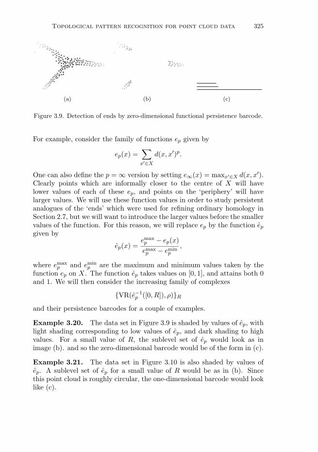
(a) (b) (c)
Figure 3.9. Detection of ends by zero-dimensional functional persistence barcode.
For example, consider the family of functions ep given by
ep(x) =∑x′∈X
d(x, x′)p.
One can also define the p =∞ version by setting e∞(x) = maxx′∈X d(x, x′).Clearly points which are informally closer to the centre of X will havelower values of each of these ep, and points on the ‘periphery’ will havelarger values. We will use these function values in order to study persistentanalogues of the ‘ends’ which were used for refining ordinary homology inSection 2.7, but we will want to introduce the larger values before the smallervalues of the function. For this reason, we will replace ep by the function epgiven by
ep(x) =emaxp − ep(x)
emaxp − emin
p
,
where emaxp and emin
p are the maximum and minimum values taken by thefunction ep on X. The function ep takes values on [0, 1], and attains both 0and 1. We will then consider the increasing family of complexes
{VR(e−1p ([0, R]), ρ)}R
and their persistence barcodes for a couple of examples.
Example 3.20. The data set in Figure 3.9 is shaded by values of ep, withlight shading corresponding to low values of ep, and dark shading to highvalues. For a small value of R, the sublevel set of ep would look as inimage (b). and so the zero-dimensional barcode would be of the form in (c).
Example 3.21. The data set in Figure 3.10 is also shaded by values ofep. A sublevel set of ep for a small value of R would be as in (b). Sincethis point cloud is roughly circular, the one-dimensional barcode would looklike (c).
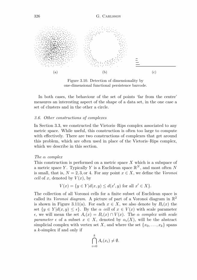
326 G. Carlsson
(a) (b) (c)
Figure 3.10. Detection of dimensionality byone-dimensional functional persistence barcode.
In both cases, the behaviour of the set of points ‘far from the centre’measures an interesting aspect of the shape of a data set, in the one case aset of clusters and in the other a circle.
3.6. Other constructions of complexes
In Section 3.3, we constructed the Vietoris–Rips complex associated to anymetric space. While useful, this construction is often too large to computewith effectively. There are two constructions of complexes that get aroundthis problem, which are often used in place of the Vietoris–Rips complex,which we describe in this section.
The α complex
This construction is performed on a metric space X which is a subspace ofa metric space Y . Typically Y is a Euclidean space RN , and most often Nis small, that is, N = 2, 3, or 4. For any point x ∈ X, we define the Voronoicell of x, denoted by V (x), by
V (x) = {y ∈ Y |d(x, y) ≤ d(x′, y) for all x′ ∈ X}.The collection of all Voronoi cells for a finite subset of Euclidean space iscalled its Voronoi diagram. A picture of part of a Voronoi diagram in R2
is shown in Figure 3.11(a). For each x ∈ X, we also denote by Bε(x) theset {y ∈ Y |d(x, y) ≤ ε}. By the α cell of x ∈ V (x) with scale parameterε, we will mean the set Aε(x) = Bε(x) ∩ V (x). The α complex with scaleparameter ε of a subset x ∈ X, denoted by αε(X), will be the abstractsimplicial complex with vertex set X, and where the set {x0, . . . , xk} spansa k-simplex if and only if
k⋂i=0
Aε(xi) = ∅.
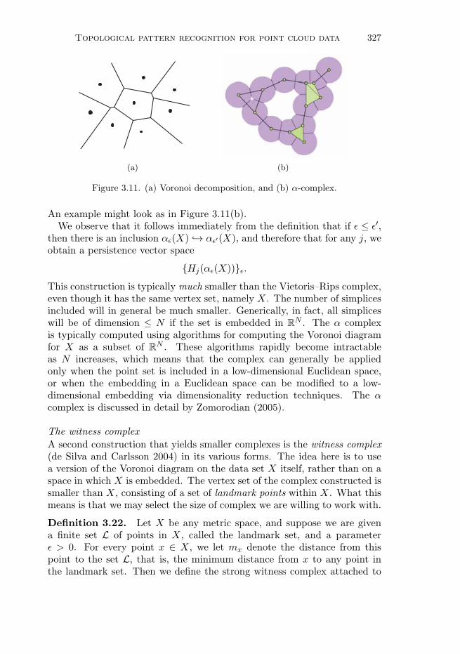
Topological pattern recognition for point cloud data 327
(a) (b)
Figure 3.11. (a) Voronoi decomposition, and (b) α-complex.
An example might look as in Figure 3.11(b).We observe that it follows immediately from the definition that if ε ≤ ε′,
then there is an inclusion αε(X) ↪→ αε′(X), and therefore that for any j, weobtain a persistence vector space
{Hj(αε(X))}ε.This construction is typically much smaller than the Vietoris–Rips complex,even though it has the same vertex set, namely X. The number of simplicesincluded will in general be much smaller. Generically, in fact, all simpliceswill be of dimension ≤ N if the set is embedded in RN . The α complexis typically computed using algorithms for computing the Voronoi diagramfor X as a subset of RN . These algorithms rapidly become intractableas N increases, which means that the complex can generally be appliedonly when the point set is included in a low-dimensional Euclidean space,or when the embedding in a Euclidean space can be modified to a low-dimensional embedding via dimensionality reduction techniques. The αcomplex is discussed in detail by Zomorodian (2005).
The witness complex
A second construction that yields smaller complexes is the witness complex(de Silva and Carlsson 2004) in its various forms. The idea here is to usea version of the Voronoi diagram on the data set X itself, rather than on aspace in which X is embedded. The vertex set of the complex constructed issmaller than X, consisting of a set of landmark points within X. What thismeans is that we may select the size of complex we are willing to work with.
Definition 3.22. Let X be any metric space, and suppose we are givena finite set L of points in X, called the landmark set, and a parameterε > 0. For every point x ∈ X, we let mx denote the distance from thispoint to the set L, that is, the minimum distance from x to any point inthe landmark set. Then we define the strong witness complex attached to
328 G. Carlsson
this data to be the complex W s(X,L, ε) whose vertex set is L, and where acollection {l0, . . . , lk} spans a k-simplex if and only if there is a point x ∈ X(the witness) so that d(x, li) ≤ mx + ε for all i. We can also consider theversion of this complex in which the one-simplices are identical to thoseof W s(X,L, ε), but where the family {l0, . . . , lk} spans a k-simplex if andonly if all the pairs (li, lj) are one-simplices. We will denote this complexby W s
VR.
There is a modified version of this construction, which is quite useful,called the weak witness construction. Suppose we are given a metric spaceX, and a set of points L ⊆ X. Let Λ = {l0, . . . , lk} denote a finite subset ofL. We say a point x ∈ X is a weak witness for Λ if d(x, l) ≥ d(x, li) for all iand all l ∈ Λ. Given ε, we will also say that x is an ε-weak witness for Λ ifd(x, l) + ε ≥ d(x, li) for all i and all l /∈ Λ.
Definition 3.23. Let X, L, and ε be as above. By the weak witnesscomplex Ww(X,L, ε) for the given data we will mean the complex whosevertex set is L, and for which a family Λ = {l0, . . . , lk} spans a k-simplex ifand only if Λ and all its faces admit ε-weak witnesses. This complex clearlyalso has a version in which a k-simplex is included as a simplex if and onlyif all its 1-faces are, and this version is denoted by Ww
VR.
One verifies directly from the definition that whenever 0 ≤ ε ≤ ε′, wethen have an inclusion
W s(X,L, ε) ↪→W s(X,L, ε′),and therefore that after applying homology, we obtain a persistence vectorspace {Hk(W
s(X,L, ε))}ε. The same applies to the variant constructionsW s
VR, Ww, and Ww
VR.
Remark 3.24. The point of introducing the complexes W sVR and Ww
VR isthat they require much less memory, since all the information is containedin the zero- and one-simplices.
3.7. Zigzag persistence
Persistence objects (sets, vector spaces, etc.) are defined by a collection ofobjects parametrized by the non-negative real line together with morphismsfrom the objects with parameter value r to objects with parameter valuer′, whenever r ≤ r′. If we restrict the persistence object to the lattice ofnon-negative integers, we can view a persistence object as a diagram
X0 → X1 → X2 → · · · → Xn → · · ·of objects Xn and morphisms Xn → Xn+1 for all n ≥ 0. We can informallystate that a persistence object restricted to the integers is equivalent to a

Topological pattern recognition for point cloud data 329
diagram of objects having the shape
0 1 2 3 4
where the nodes are objects (sets, vector spaces, simplicial complexes, . . . ),and the arrows indicate a morphism from one object to another. As such,it is an infinite quiver diagram (Derksen and Weyman 2005). Any directedgraph Γ is called a quiver, and a representation of Γ over a field k is anassignment of a k-vector space Vv to each vertex of Γ and a k-linear trans-formation Le : Vv → Vw for every edge e from v to w. We will also referto a representation of Γ as a diagram of shape Γ. One could also considerdiagrams with the shape
0 1 2 3 4
Precisely, this corresponds to a family of objects parametrized by the non-negative integers, with a morphism from Xi → Xi+1 when i is even, and amorphism Xi+1 → Xi when i is odd. We will call such a diagram of k-vectorspaces, where k is a field, a zigzag persistence vector space. Zigzag vectorspaces arise in a number of ways.
Example 3.25. Consider a very large finite metric space X, so large thatwe do not expect to be able to compute its persistent homology using aVietoris–Rips complex. We might instead try to form many smaller samples{Si} from X, and attempt to understand how consistent these calculationsare. We note that given such a family of samples, we may fix a thresholdparameter R and construct VR(Si, R) for all i. To attempt to assess theconsistency of the computations which arise out of these complexes, we canform the unions Si ∪ Si+1 and note that we have inclusion maps Si ↪→Si ∪ Si+1 and Si+1 ↪→ Si ∪ Si+1. These maps induce maps on the Vietoris–Rips complexes, and by applying homology to the Vietoris–Rips complexes,we obtain k-vector spaces Vi = Hj(VR(Si, R)) and Vi,i+1 = Hj(VR(Si ∪Si+1, R). The inclusion maps now mean that we obtain a diagram of theform
V0 → V0,1 ← V1 → V1,2 ← V2 → V2,3 ← V3 → · · · .On an intuitive level, consistency between the calculations is measured bythe existence of classes xi ∈ Vi and xi+1 ∈ Vi+1, so that the images of xi andxi+1 in Vi,i+1 are the same non-zero class, and more generally for sequencesof classes {xi}, with xi ∈ Vi, so that for all i, the images of xi and xi+1 inVi,i+1 are equal to the same non-zero element.
Example 3.26. Given a simplicial complex X and a simplicial map fromX to the non-negative real line, triangulated, with the vertex set being the

330 G. Carlsson
non-negative integers and the edges being the closed intervals [n, n+1], wecan form the subcomplexes f−1([n, n+ 1]), as well as f−1(n). We have thediagram
f−1(0)→ f−1([0, 1])← f−1(1)→ f−1([1, 2])← f−1(2)→ · · ·A scheme which could compute homology only of complexes based at thenodes of this diagram, and which could extract the homology of the entirecomplex from these calculations, would permit the parallelization of homol-ogy computations into smaller pieces. This is of course very desirable.
Example 3.27. In the discussion of the witness complex, we selected aset of landmarks L from a metric space X, and computed certain complexesW (X,L, ε), for which there were several variants. We suppress the super-scripts s and w, as well as the other labels, since the construction worksfor all the values. In general, it is difficult to assess how accurately thepersistent homology of X is captured by the witness complex. One pieceof evidence for accuracy would be a method which assesses how consistentdifferent choices of landmarks are. In order to do this, one can constructa bivariate version of the witness complex which takes as input a pair oflandmark sets (L1,L2), denoted by W (X, (L1,L2), ε), which maps to eachof the complexes W (X,L1, ε) and W (X,L2, ε) in a natural way. Given acollection of landmark sets Li, we obtain a diagram of witness complexes
W (X,L1, ε)←W (X, (L1,L2), ε)→W (X,L2, ε)← .
After applying homology, one can again ask for consistent families as inExample 3.25 above.
It now turns out that there is a classification theorem for zigzag persis-tence vector spaces over a field k analogous to that for ordinary persistence.
Definition 3.28. A zigzag persistence k-vector space V. is called cyclic ifthere are integers m ≤ n so that Vi = k for m ≤ i ≤ n, Vi = {0} if i < m ori > n, and the homomorphisms Vi → Vi+1 or Vi+1 → Vi are all equal to theidentity homomorphism on k whenever m ≤ i ≤ i+ 1 ≤ n.
One example is
{0} → kid← k
id→ k ← {0} → {0} ← · · · .Each cyclic persistence vector space is indecomposable, in that it cannotbe expressed as a direct sum of diagrams. Note that the cyclic zigzagpersistence vector spaces are parametrized by intervals [m,n] with inte-ger endpoints. We write V [m,n]. for the cyclic k-vector space which isexactly non-zero for the integers in [m,n]. We have the following analogueof Proposition 3.12.
Topological pattern recognition for point cloud data 331
Theorem 3.29. We say that a zigzag persistence k-vector space V. is offinite type if (a) each vector space Vi is finite-dimensional, and (b) Vi = {0}for sufficiently large i. Then, for any zigzag persistence k-vector space V. offinite type, there is an isomorphism
V.∼=
⊕i
V [mi, ni]. (3.2)
for some choices of pairs of integers (mi, ni). Furthermore, the decomposi-tion (3.2) is unique up to a reordering of the summands.
The content of this theorem is that there is a barcode description of theisomorphism classes of zigzag persistence vector spaces, just like that forordinary persistence vector spaces, except that the intervals in the bar-codes are constrained to be integers. This theorem was first proved byGabriel (1972), and is discussed from the point of view of computationalissues by Carlsson and de Silva (2010). This result can now be applied toExamples 3.25 and 3.27 above. The presence of long bars in the barcodedecomposition says that there are elements which are consistent across allthe vector spaces in the interval determined by the bar. For Example 3.26above, the zigzag construction can be used to give a very efficient and paral-lelizable method for computing the homology of the entire complex. Theseideas are discussed by Carlsson and de Silva (2010) and Carlsson, de Silvaand Morozov (2009).
4. Structures on spaces of barcodes
4.1. Metrics on barcode spaces
We have now associated to any finite metric space a family of persistencebarcodes, or persistence diagrams. One important property to understandis the degree to which the barcode changes when we have small (in a suitablesense) changes in the data. In order to even formulate the answer to sucha question, we will need to define what is meant by small changes in thebarcode. In order to do this, we will define the bottleneck distance betweenbarcodes. For any pair of intervals I = [x1, y1] and J = [x2, y2], we willdefine ∆(I, J) to be the l∞-distance between the two, regarded as orderedpairs in R2, that is, max(|x2− x1|, |y2− y1|). For a given interval I = [x, y],we also define λ(I) to be (y − x)/2. λ(I) is the l∞-distance to the closestinterval of the form [z, z] to I. Given two families I = {Iα}α∈A and J ={Jβ}β∈B of intervals, for finite sets A and B, and any bijection θ from asubset A′ ⊆ A to B′ ⊆ B, we will define the penalty of θ, P (θ), to be
P (θ) = max(maxa∈A′(∆(Ia, Jθ(a))
), maxa∈A−A′(λ(Ia)), max
b∈B−B′(λ(Jb)))
332 G. Carlsson
and then define the bottleneck distance d∞(I, J) to be
minθ
P (θ),
where the minimum is taken over all possible bijections from subsets of Ato subsets of B. This is easily verified to be a distance function on the setof barcodes.
Remark 4.1. d∞ is actually the p =∞ version of a family of metrics dp,called the Wasserstein metrics. The metric dp is defined via the penaltyfunction Pp, given by
Pp(θ) =∑α∈A′
∆(Iα, Jθ(α))p +
∑α∈A−A′
λ(Iα)p +
∑b∈B−B′
λ(Jb)p,
and we set dp(I, J) = (minθ Pp(θ))1p .
We now have a notion of what it means for barcodes to be close. Thereis also a notion of what it means for two compact metric spaces to be close,given by the Gromov–Hausdorff distance, first defined by Burago, Buragoand Ivanov (2001). It is defined as follows. Let Z be any metric space, andlet X and Y be two compact subsets of Z. The Hausdorff distance betweenX and Y , dH(X,Y ), is defined to be the quantity
max{maxx∈X
miny∈Y
dZ(x, y),maxy∈Y
minx∈X
dZ(x, y)}.
Given any two compact metric spaces X and Y , we consider the familyI(X,Y ) of all simultaneous isometric embeddings of X and Y . An ele-ment of I(X,Y ) is a triple (Z, iX , iY ), where Z is a metric space and iXand iY are isometric embeddings of X and Y , respectively, into Z. TheGromov–Hausdorff distance of X and Y is now defined to be the infimumover I(X,Y ) of dH(im(iX), im(iY )). It is known to give a metric on the col-lection of all compact metric spaces. It is also known to be computationallyvery intractable. Chazal et al. (2009) have proved the following.
Theorem 4.2. Fix a non-negative integer k, let F denote the metric spaceof all finite metric spaces, and let B denote the set of all persistence barcodes.Let βk : F → B be the function which assigns to each finite metric space itsk-dimensional homology barcode. Then βk is distance non-increasing.
This result is interesting not only because it gives some guarantees onhow certain changes in the data affect the result, but it also provides aneasily computed lower bound on the Gromov–Hausdorff distance in a greatdeal of generality.There are also stability results for functional persistence, or rather, an
analogue of functional persistence. In Definition 3.18, we defined functionalpersistence based on a function defined on the points of a metric space, or
Topological pattern recognition for point cloud data 333
equivalently on the vertices of its Vietoris–Rips complex. For any topo-logical space X and continuous real-valued function f : X → R, one canalso define associated persistence vector spaces {Hi(f
−1((−∞, r])}r, whichare very close analogues to the simplicial complex construction describedabove. In fact, a real-valued function on the vertex set of a simplicial com-plex can be extended in a natural way to a continuous function on thegeometric realization of the simplicial complex, using a weighted sum ofvalues of the function on the vertices based on the barycentric coordinatesof the point. The idea will be that small changes in the function shouldyield only small changes in the associated persistence barcode. The resultswe will describe appear in Cohen-Steiner, Edelsbrunner and Harer (2007)and Cohen-Steiner, Edelsbrunner, Harer and Mileyko (2010).To state the results, we will need some definitions. Let X be a topological
space, and let f : X → R be a real-valued function on X. For every non-negative integer k, a ∈ R, and ε ∈ (0,+∞), we have the induced map
j = jk,a,ε : Hk(f−1(−∞, a− ε]) −→ Hk(f
−1(−∞, a+ ε]).
We say that a is a homological critical value of f if there is a k such thatjk,a,ε fails to be an isomorphism for all sufficiently small ε. Further, we saythat the function f is tame if it has a finite number of homological criticalvalues and the homology groups Hk(f
−1(−∞, a]) are finite-dimensional forall k ∈ N and a ∈ R. This condition holds, for example, in the case of Morsefunctions on closed manifolds (see Milnor (1963)) and for piecewise linearfunctions on finite simplicial complexes, so the result we will state is quitegenerally applicable. The following theorem is proved in Cohen-Steiner et al.(2007).
Theorem 4.3. Let X be any space which is homeomorphic to a simplicialcomplex, and suppose f, g : X → R are continuous tame functions. Thenthe persistence vector spaces {Hk(f
−1((−∞, r])}r and {Hk(g−1((−∞, r])}r
are finitely presented, and therefore admit barcode descriptions for eachk ∈ N, which we denote by βkf and βkg. Moreover, for any k, we have that
d∞(βkf, βkg) ≤ ‖f − g‖∞.
There is also a stability result for the Wasserstein distances dp, with pfinite, in the presence of a Lipschitz property for the functions, proved inCohen-Steiner et al. (2010).
4.2. Coordinatizing barcode space
Another way to describe infinite sets is via the theory of algebraic varieties,that is, as the set of solutions to a set of equations, either over the realnumbers, the complex numbers, or some other field. When this is possible,it gives a very compact description of a large or infinite set. The method
334 G. Carlsson
also produces a ring of functions on the set, by restricting the polynomialfunctions to it. Functions are useful in studying any set by machine learn-ing and other methods. We will discuss the possibilities for producing acoordinatized model of the set of all barcodes.Let us consider first the set Bn of all barcodes containing exactly n inter-
vals or ‘bars’. Each of the intervals is determined by two coordinates, theleft-hand endpoint x and the right-hand endpoint y. If we have n intervals,we have 2n coordinates {x1, y1, . . . , xn, yn}. The trouble is that the barcodespace does not take into account the ordering of the intervals, so it is notpossible to assign a value to the ith coordinate itself. To understand howto get around this problem, we discuss a familiar situation from invarianttheory.We consider Rn, let Σn be the group of permutations of the set {1, . . . , n},
and consider the ring of polynomial functions An = R[x1, . . . , xn] on Rn. Wewill describe how to coordinatize the set of orbits (as defined in Section 2.2)Rn/Σn, that is, the ‘set of unordered n-tuples of real numbers’, or equiva-lently the collection of multisets of size n. If f is a polynomial function onRn, it may be treated as a function on the set of orbits if it has the propertythat f(σ�v) = f(�v) for all σ ∈ Σn and �v ∈ Rn. The group Σn acts on thering An, and an element f ∈ An is a function on the orbit set Rn/Σn ifand only if it is fixed under all permutations σ ∈ Σn. The set of all fixedfunctions (denoted by AΣn
n ) is a ring in its own right, and it turns out thatit has a very simple description.
Proposition 4.4. The ring AΣnn is isomorphic to the ring of polynomials
R[σ1, σ2, . . . , σn], where σi denotes the ith elementary symmetric functiongiven by ∑
s1,s2,...,si
xs1xs2 · · ·xsi ,
where the sum is over all i-tuples of distinct elements of {1, . . . , n}.
We now have coordinates that describe the set R/Σn. The analogous con-struction for the set Bn would be to form the subring of R[x1, y1, . . . , xn, yn]fixed under the action of Σn which permutes the xi among themselves andthe yi among themselves, and obtain a coordinatization in this way. Thisdoes give a ring of functions, but it is not a pure polynomial ring but hasrelations, or syzygies. A full discussion of this situation is given in Dalbec(1999). To give an idea of what this means, we first observe that the ele-mentary symmetric functions σi(�x) and σi(�y) are definitely invariant, andgenerate a full polynomial subring of the ring of functions. Let us restrictto the case n = 2. Then there is another function ξ = (x1y1 + x2y2), whichcannot be expressed in terms of the elementary symmetric functions applied
Topological pattern recognition for point cloud data 335
to �x and �y. It turns out that there is now an algebraic relation
ξ2 − σ1(�x)σ1(�y)ξ + σ1(�x)2σ2(�y) + σ2(�x)σ1(�y)
2 − 4σ2(�x)σ2(�y) = 0,
which after consideration shows that there is no algebraic coordinatizationby the four-dimensional affine space but rather by a subset of a higher-dimensional space defined by one or more algebraic equations. Nevertheless,one can express Bn as the points of an algebraic variety in this way.What we would really like to do is to coordinatize the collection of all the
setsBn as a variety, in an appropriate sense. One could consider the disjointunion
∐nBn, but we would rather disregard intervals of length zero in a
systematic way, since they correspond to features which are born and die atthe same time, and hence do not have any actual persistence. This suggeststhat we define a set B∞ as follows. We let ∼ denote the equivalence relationon
∐nBn generated by equivalences
{[x1, y1], [x2, y2], . . . , [xn, yn]} ∼ {[x1, y1], [x2, y2], . . . , [xn−1, yn−1]}whenever xn = yn. We then define the infinite barcode set B∞ to be thequotient ∐
n
Bn/ ∼ .
The question we now pose is whether this infinite set can also be coordina-tized, again in a suitable sense. To see how this can be done, we considertwo simpler examples of coordinatization.
Example 4.5. We let An denote the set Rn/Σn, and we let A∞ denote∐n
An/ ∼,
where ∼ is the equivalence relation given by declaring that (x1, . . . , xn) ∼(y1, . . . , ym) if and only there are sets S ∈ {1, . . . , n} and T ⊆ {1, . . . ,m}satisfying the following properties.
(1) xs = 0 and yt = 0 for all s ∈ S and t ∈ T .
(2) We have n−#(S) = m−#(T ), and call this common number k.
(3) The unordered k-tuples obtained by deleting the elements correspond-ing to S and T from (x1, . . . , xn) and (y1, . . . , ym) respectively, areidentical.
There are natural maps from An to A∞, and the maps are injective onpoints. We therefore have an increasing system
A1 ↪→ A2 ↪→ A3 ↪→ · · · ,which corresponds to a system of ring homomorphisms
R[σ1]← R[σ1, σ2]← R[σ1, σ2, σ3]← · · · ,
336 G. Carlsson
where the homomorphism R[σ1, . . . , σn+1] → R[σ1, . . . , σn] is defined byσi → σi for 1 ≤ i ≤ n, and σn+1 → 0.Associated to such a system is its limit, which is itself a ring. We will
not go into detail about this, but refer to the book by Mac Lane (1998)for background material on limits and their dual construction, a colimit.In this case, the construction produces a ring of functions which can bedescribed as follows. LetM denote the set of all monomials in the infiniteset {σ1, σ2, . . . , σn, . . .}, and let Mn ⊆ M denote the subset of monomialswhich involve only {σ1, . . . , σn}. Then inverse limit ring is identified withthe set of all infinite sums
∑µ∈M rµµ so that the sums
∑µ∈Mn
rµµ are
all finite. So, for instance, the infinite sum∑
n σn is an element of thisring. Elements in this ring certainly define functions on A∞, because thefunctions σN vanish on An whenever n ≤ N . The limit ring is, however, alittle complicated given the finiteness conditions we are required to impose.It would be simpler to restrict in a natural way to the functions which arepolynomial in the elements σi. One way to do this is as follows. We mayextend the rings R[σ1, . . . , σn] to have complex coefficients, so that they areof the form C[σ1, . . . , σn], and construct the limit ring Λ as in the real case.The group of complex numbers of length one now acts on this ring via theaction defined by
ζ · (σi) = ζiσi
and extended to the limit ring in the obvious way. We say that an elementf in Λ is K-finite if the span of the entire orbit of f is a finite-dimensionalC-vector space. (The notion of K-finiteness is introduced in Knapp.) Theintersection of the set of K-finite vectors in Λ with the limit ring over R cannow be identified with the polynomial ring on the variables σi.
In the example above, taking the quotient by the equivalence relation ∼did not create complicated rings, as each of the rings R[σ1, σ2, . . . , σn] is apure polynomial ring in n variables. In general, though, taking quotients byequivalence relations can create rings which are not pure polynomial, andin some cases not even finitely generated as algebras.
Example 4.6. Consider the plane X = R2, and consider the equivalencerelation ∼ defined by declaring that (x, 0) ∼ (x′, 0) for all x, x′. This relation‘collapses’ the entire x-axis to a point, while leaving the rest of the setunchanged. The question is whether or not R2/ ∼ can be described as analgebraic variety. As in the case of the ring of invariants of a group actiongiving a variety structure on an orbit set, in this case we will ask whichpolynomial functions f on R have the property that f(x) = f(x′) wheneverx ∼ x′. This means that we are asking for the polynomials f in two variablesso that f(x, 0) = f(x′, 0) for all x, x′. A quick calculation shows that thisring of functions consists of all polynomials in x and y so that the linear term

Topological pattern recognition for point cloud data 337
in x is zero. So, a basis for it is the set of monomials {xiyj |i > 0 =⇒ j > 0}.This is a ring which is easy to understand, but it is not a finitely generatedalgebra. It is generated by the elements θi = xiy together with the elementy, and they satisfy the relations θ2i = yθ2i. We can then obtain a descriptionof R2/ ∼ as the set of points in R∞ = {(y, θ1, θ2, . . .)|θ2i = yθ2i for all i > 0}.Note that in this case infinitely many coordinates will typically be non-zerofor a given (x, y).
The image of Bn → B∞, which we denote by B′n, can be described as
the set obtained from Bn by taking the quotient by an equivalence relation∼n defined as follows. Given two multisets of intervals (with n intervals)S = {[x1, y1], [x2, y2], . . . , [xn, yn]} and S′ = {[x′1, y′1], [x′2, y′2], . . . , [x′n, y′n]},we say that S ∼n S′ if there are subsets I, I ′ ⊂ {1, . . . , n}, so that xi =yi for all i ∈ I, and x′i′ = y′i′ for all i′ ∈ I ′, and so that the multisetsS − {[xi, xi]|i ∈ I} and T − {[x′i′ , x′i′ ]|i′ ∈ I ′} are identical multisets ofintervals. This means that B′
n can be expressed as the quotient of Bn
by an equivalence relation, similar to that described in Example 4.6. Itcorresponds to a ring A(B′
n), which is in general not finitely generated.However, we consider the increasing sequence of sets
B′1 ↪→ B′
2 ↪→ B′3 ↪→ · · ·
and a corresponding system of ring homomorphisms
A(B′1)←− A(B′
2)←− A(B′3)←− · · · ,
as in Example 4.5. This system also has a limit, which we will denote byA(B∞). There is a construction of K-finite vectors analogous to the onecarried out above in the case of the symmetric polynomials, and the ring ofK-finite vectors turns out to be isomorphic to a polynomial ring on a setof variables {τij |1 ≤ i, 0 ≤ j}. The variables τij correspond to functions onB∞, which can be described as follows. It will suffice to describe τij on Bn,that is, on an unordered n-tuple of intervals. To do this, we first define afunction τ ′ij on the set of ordered n-tuples on intervals by
τ ′ij([x1, y1], . . . , [xn, yn]) = (y1 − x1) · · · (yi − xi)
(y1 + x1
2
)j
.
To obtain τij we simply symmetrize by writing
τij =∑σ∈Σn
τ ′ij ◦ σ.
So, for example, τ10 applied to an unordered n-tuple of intervals is the sum ofthe lengths of the intervals, τ20 is the second elementary symmetric functionin the lengths, and τ1j is the sum over all the intervals of the product of thelength of the interval with the jth power of its midpoint.

338 G. Carlsson
Figure 4.1. A loop with outliers.
4.3. Multidimensional persistence
One of the problems which frequently comes up in persistent homologicalcalculations is that the presence of a few outliers can mask structure. Theexample in Figure 4.1 is suggestive. Note that the main structure is asampling from a loop, but there are a number of outliers in the interior ofthe loop. The homology of the complexes built from this data set will notstrongly reflect the loop, because the short connections among the outliersand between the outliers and the points on the actual loop will quickly fillin a disc. In order to remedy this, we would have to find a principled wayto remove the outliers in the interior. A measure of density would have thiseffect, because the outliers by many measures of density would have muchlower density than the points on the loop itself. So, if we selected, say, the90% densest points by a density measure, we would effectively be choosingthe loop itself. However, this choice of threshold is arbitrary, so just as wechose to maintain a profile of homology groups over all threshold values forthe scale parameter, we might attempt to create such a profile for valuesof density.Another problem with persistent homology has already been made appar-
ent in Section 3.5, where we constructed the increasing family of simplicialcomplexes {VR(f−1([0, R]), ρ}R for a non-negative real-valued function fon our data set, and for a fixed choice of our scale parameter ρ. These com-plexes allowed us to study topological features of the data sets which are notcaptured by the direct application of persistent homology, but using themrequires us to make a choice of the scale parameter. There is no universalor natural choice of ρ, so it would be very desirable to be able to track bothR and ρ simultaneously.
These considerations motivate the following definition. We let R+ =[0,+∞), and we define a partial order on Rn
+ by declaring that (r1, . . . , rn) ≤(r′1, . . . , r′n) if and only if ri ≤ r′1 for all 1 ≤ i ≤ n.

Topological pattern recognition for point cloud data 339
Definition 4.7. By an n-persistence vector space over a field k, we willmean a family of k-vector spaces {V�r}�r∈Rn together with linear transforma-tions L(�r, �r′) : V�r → V�r′ whenever �r ≤ �r′, so that
L(�r′, �r′′) · L(�r, �r′) = L(�r, �r′′)
whenever �r ≤ �r′ ≤ �r′′. There are obvious notions of linear transformationsand isomorphisms of n-persistence vector spaces.
We might hope that there is a compact representation of the isomorphismclasses of n-persistence vector spaces analogous to the barcode or persistencediagram representations available in 1-persistence, equivalently the ordinarypersistence we have already discussed. It turns out, though, that this is notpossible, for the following reason. As was observed in Zomorodian andCarlsson (2005), ordinary persistence vector spaces have much in commonwith the classification of graded modules over the graded ring k[t]. Indeed,if we restrict the domain of the scale parameter r in ordinary persistence tothe integer lattice Z+ ⊆ R+, then the classification of such restricted persis-tence vector spaces is identical to the classification of graded k[t]-modules.Similarly, it is shown in Carlsson and Zomorodian (2009) that the isomor-phism classification of n-persistence vector spaces with the parameter setrestricted to Zn
+ is identical to the classification of n-graded modules overthe n-graded ring k[t1, . . . , tn]. It is well understood in algebraic geometrythat the classification of modules over polynomial rings in more than onevariable is fundamentally different from the one-variable case. In particular,for graded one-variable polynomial rings, the parametrization of the set ofisomorphism classes is independent of the underlying field k, whereas thisdoes not hold for multigraded polynomial rings in more than one variable.In fact, the classification for more than one variable usually involves spacesof structures, rather than discrete sets. What these problems suggest is thatwe should drop the idea of dealing with a complete classification of the iso-morphism classes of n-persistence vector spaces, and instead develop usefulinvariants which we expect will measure useful and interesting properties ofn-persistence vector spaces.One approach to finding invariants is via the functions defined in Sec-
tion 4.2. It turns out that some of them can be interpreted in ways whichdo not depend on obtaining an explicit barcode representation. For anyfinitely presented persistence vector space {Vr}r, we can define two func-tions attached to V , ∆V : R+ → R+ and ρV : R2
+ → R+. We set
∆V (r) = dim(Vr)
and
ρV (r, r′) = rank(L(r, r′)).
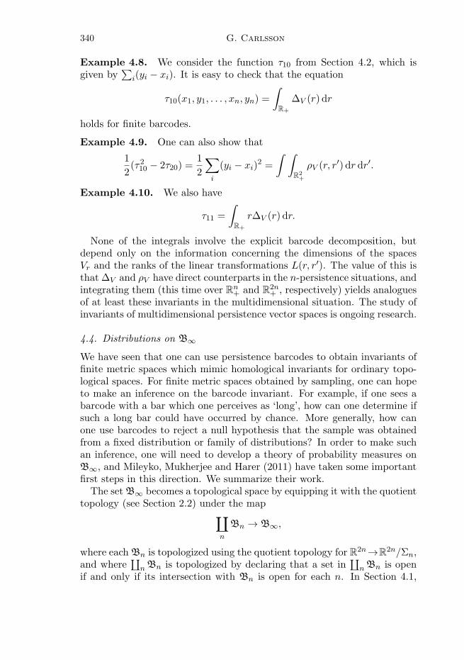
340 G. Carlsson
Example 4.8. We consider the function τ10 from Section 4.2, which isgiven by
∑i(yi − xi). It is easy to check that the equation
τ10(x1, y1, . . . , xn, yn) =
∫R+
∆V (r) dr
holds for finite barcodes.
Example 4.9. One can also show that
1
2(τ210 − 2τ20) =
1
2
∑i
(yi − xi)2 =
∫ ∫R2+
ρV (r, r′) dr dr′.
Example 4.10. We also have
τ11 =
∫R+
r∆V (r) dr.
None of the integrals involve the explicit barcode decomposition, butdepend only on the information concerning the dimensions of the spacesVr and the ranks of the linear transformations L(r, r′). The value of this isthat ∆V and ρV have direct counterparts in the n-persistence situations, andintegrating them (this time over Rn
+ and R2n+ , respectively) yields analogues
of at least these invariants in the multidimensional situation. The study ofinvariants of multidimensional persistence vector spaces is ongoing research.
4.4. Distributions on B∞
We have seen that one can use persistence barcodes to obtain invariants offinite metric spaces which mimic homological invariants for ordinary topo-logical spaces. For finite metric spaces obtained by sampling, one can hopeto make an inference on the barcode invariant. For example, if one sees abarcode with a bar which one perceives as ‘long’, how can one determine ifsuch a long bar could have occurred by chance. More generally, how canone use barcodes to reject a null hypothesis that the sample was obtainedfrom a fixed distribution or family of distributions? In order to make suchan inference, one will need to develop a theory of probability measures onB∞, and Mileyko, Mukherjee and Harer (2011) have taken some importantfirst steps in this direction. We summarize their work.The setB∞ becomes a topological space by equipping it with the quotient
topology (see Section 2.2) under the map∐n
Bn → B∞,
where eachBn is topologized using the quotient topology for R2n→R2n/Σn,and where
∐nBn is topologized by declaring that a set in
∐nBn is open
if and only if its intersection with Bn is open for each n. In Section 4.1,

Topological pattern recognition for point cloud data 341
metrics dp, with the possibility of p =∞, were introduced on B∞. The goalof the work in Mileyko et al. (2011) is to study the possibility of definingexpectations and variances, in the Frechet sense (Frechet 1944, 1948), onthe metric spaces (B∞, dp). One obstacle to realizing this goal is the factthat the metric space (B∞, dp) is not complete. In order to deal with this
problem, Mileyko et al. (2011) construct completions Bp of (B, dp). We willfirst enlarge the set B∞ to include countable multisets of intervals {Ia}a∈A,where A is a countable set. For a fixed p, the underlying set of Bp will bethe set of all {Ia}a∈A for which∑
a∈Aλ(Ia) < +∞. (4.1)
It is now clear by inspection that the distance dp extends naturally to a
metric dp on Bp via the same formula as in Section 4.1: the sum may beinfinite, but it is always convergent due to condition (4.1). We now havethe following.
Theorem 4.11 (Mileyko et al. 2011). The metric space (Bp, dp) is com-plete and separable.
The goal of Mileyko et al. (2011) is now to construct means and variances
on Bp. In general metric spaces X there is no notion of a single point-valuedmean, but the mean will actually be a subset of X. Here is the definitionof Frechet means and variances, paraphrased from Mileyko et al. (2011).
Definition 4.12. Let X be a metric space, let B(X) be its Borel σ-algebra, and let P be a probability measure on (X,B(X)), and supposethat P has a finite second moment, that is,
∫X d(x, x′)2 dP(x′) <∞ for all
x ∈ X. Then, by the Frechet variance of P we will mean
varP = infx∈X
[FP(x) =
∫X
d(x, x′)2 dP(x′)],
and the set
EP = {x|FP(x) = varP}will be called the Frechet expectation or the Frechet mean of P.As stated, EP always exists as a set, but it may be empty or contain more
than one point. There are results on the non-emptiness and the uniquenessof Frechet means for manifolds (Karcher 1977, Kendall 1990). What is
proved in Mileyko et al. (2011) is an existence result for the case X = Bp.
Theorem 4.13. Let P be a probability measure on (Bp, dp), and supposethat P has finite second moment and compact support. Then EP = ∅.

342 G. Carlsson
Turner, Mileyko, Mukherjee and Harer (2014) made this existence theo-rem algorithmic, but for a somewhat different choice of metric and metricspace. By the L2 Wasserstein metric on B∞, we mean the analogue of d2for the choice of penalty function
λL2(I, J) = (x1 − x2)2 + (y1 − y2)
2.
The resulting metric space is simpler to work with computationally, and allthe existence results from Mileyko et al. (2011) are also shown to hold inTurner et al. (2014).Another approach concerns the notion of distances between measures on
metric spaces, and developed by Blumberg, Gal, Mandell and Pancia (2013)and Chazal, Cohen-Steiner and Merigot (2011). One useful choice is the so-called Levy–Prohorov metric.
Definition 4.14. Given a metric space (X, dX), the Levy–Prohorov met-ric πX on the set P(X) of probability measures on the measurable space X,with its σ-algebra of Borel sets B(X), is defined by
πX(µ, ν) =
inf{ε > 0|µ(A) ≤ ν(Aε) + ε and ν(A) ≤ µ(Aε) + ε for all A ∈ B(X)},where Aε denotes the ε-neighbourhood of A, that is, the union of all balls ofradius ε about points of A. This metric is defined for all metric spaces, andis known to induce the topology of weak convergence of measures on P(X)when X is a ‘Polish space’, that is, a separable complete metric space.
By a metric measure space (X, dX , µX), we will mean a metric space(X, dX) together with a probability measure µX on the σ-algebra of Borelsets associated to the metric dX . Greven, Pfaffelhuber and Winter (2009)defined an analogue to the Gromov–Hausdorff metric on the collection ofcompact metric measure spaces. Given two metric measure spaces
X = (X, dX , µX) and Y = (Y, dY , µY ),
the Gromov–Prohorov distance between X and Y is defined by Greven et al.(2009) to be
dGPr(X ,Y) = inf(ϕX ,ϕY ,Z)
π(Z,dZ)((ϕX)∗µX , (ϕY )∗µY )
where, as in the definition of the Gromov–Hausdorff metric, (ϕX , ϕY , Z)varies over all pairs of isometric embeddings ϕX : X → Z and ϕY : Y → Zof X and Y into a compact metric space Z.The distributions on B∞ of interest in Blumberg et al. (2013) are those
which are obtained by sampling n points in X, according to the probabilitymeasure µX , and computing persistent homology in a fixed dimension kto obtain persistence barcodes. The idea is that each one is a kind of
Topological pattern recognition for point cloud data 343
finite approximation to the metric measure space, and the result showsthat the differences between these measures is controlled by the Gromov–Prohorov distance between the actual metric spaces. More precisely, givena metric measure space (X, dX , µX), they construct probability measures
Φnk = Φn
k(X, dX , µX) on the completed barcode spaces B∞ described above,via the formula
Φnk(X, dX , µX) = (βk)∗(µn
X),
where βk denotes the k-dimensional barcode, and (−)∗ denotes the push
forward measure to Bp. This formula makes sense because (a) βk is acontinuous map of metric spaces by Theorem 4.2, and (b) both spaces aregiven the structure of measurable spaces via the Borel σ-algebras. The maintheorem of Blumberg et al. (2013) is now as follows.
Theorem 4.15 (Blumberg et al. 2013, Theorem 5.2). Let (X, dX , µX)and (Y, dY , µY ) be compact metric measure spaces. Then we have the fol-lowing inequality relating the Prohorov and Gromov–Prohorov metrics:
πB∞(Φnk(X, dX , µX),Φn
k(Y, dY , µY )) ≤ ndGPr((X, dX , µX), (Y, dY , µY )).
This estimate permits us to prove the following convergence result.
Corollary 4.16 (Blumberg et al. 2013, Corollary 5.5). Let S1 ⊂ S2
⊂ · · · ⊂ · · · be a sequence of randomly drawn samples from (X, dX , µX).We regard Si as a metric measure space using the subspace metric and theempirical measure. Then Φn
k(Si) converges in probability to Φnk(X, dX , µX).
Remark 4.17. One could formulate similar results in other contexts. Forexample, a very interesting object of study would be to study the distri-butions obtained by instead choosing various landmark sets in a witnesscomplex. This would then give an assessment of how well the space is rep-resented by witness complexes of a fixed size.
5. Organizing data sets
5.1. Natural image patches
In this section we will describe the homological analysis of a particular dataset coming out of neuroscience and image processing. The data set wasconstructed by Lee, Pedersen and Mumford (2003), and the analysis wasdone by Carlsson, Ishkhanov, de Silva and Zomorodian (2008). We firstdiscuss the data set. It consists of images from a black and white digitalcamera. Each such image can be thought of as a pixel vector in a spacewhose dimension is the number of pixels used in the camera, and wherethe coordinate for a given pixel is a grey-scale value, which we will think ofas a continuous variable, but which in fact takes integer values between 0
344 G. Carlsson
and 255. The ‘metaproblem’ proposed by Lee et al. was to understand insome sense the structure of the set of all images that might actually occurin taking images, versus the set of all possible pixel vectors. The usualtopological method of trying to understand a space makes little sense here,due to the extremely high dimensionality of the space of images. Lee et al.decided instead to study the statistics of small (3×3) patches within a largedatabase of images taken by two Dutch neuroscientists around Groningenin the Netherlands (van Hateren and van der Schaaf 1998).Each such patch was taken as a vector in R9, with one grey-scale value
for each of the nine pixels. One preliminary observation is that most imagescontain large solid regions, and therefore that patches which are constantor nearly constant will dominate the statistics of the set of patches. Forthis reason, Lee et al. decided to study only high-contrast patches, that is,patches {xij}1≤i,j≤3 such that a certain positive definite quadratic form onthe vector of differences {xij −µ} is large, where µ is the mean value of thevalues xij . The quadratic form is called the D-norm, and is a rescaling ofthe standard Euclidean form in a way which reflects the placement of thepixels in the 3× 3 array. They then constructed a data set of 4× 10⁶ high-contrast patches, by which they mean patches whose D-norm lies in thetop 20% values which occur. They then proceeded to perform the followingtransformations to this data set.
(1) For any vector �x = {xij}ij , let µ(�x) denote the mean of the entriesxij . Replace each vector �x by �x′ = �x − µ(�x). This is done so asto understand the structure of the patch independent of the absolutevalues of the grey-scale values.
(2) Replace each vector �x′ by �x′/‖�x′‖D. This is done so as to understandthe patch structure independently of the absolute value of the contrastin the patch.
We now have a data setM consisting of 4× 10⁶ points lying on a seven-dimensional ellipsoid E7 within an eight-dimensional subspace of R9. Thisis the data set we will study.The first inclination is to apply persistent homology directly. Unfortu-
nately, it turns out thatM fills out the full E7, which would mean that werewe to carry out the calculation, we would expect to find the homology ofE7. This would be unsurprising, and would not yield useful insights aboutM. One can observe, though, that the density suitably measured varies agreat deal within M. This means that we can threshold by density, andobtain a data set consisting of the most frequently appearing patches, ormotifs, in M. Such information would clearly be useful, for example, inconstructing compression schemes. The analysis in Carlsson et al. (2008)

Topological pattern recognition for point cloud data 345
(a) (b)
β0 β1
0 0.1 0.2 0.3 0.4 0.5 0.6 0 0.1 0.2 0.3 0.4 0.5 0.6
Figure 5.1. (a) Zero-dimensional and (b) one-dimensionalpersistence barcodes for X(300, 30).
Figure 5.2. Primary circle in the data setM.
uses a very simple proxy for density, called co-density. The co-density withparameter k on a finite metric space, denoted by ρk(x), is defined by
ρk(x) = {d(x, x′)| where x′ is the kth nearest neighbour to x}.Note that ρk varies inversely with actual density, and also that the parameterk plays a role similar to the choice of variance in a Gaussian kernel densityestimator. The size of the parameter k determines whether the density iscomputed more or less locally, that is, using smaller or larger balls around apoint x. For a data set X, we let X(k, p), where k is a positive integer andp is a percentage, denote the set of points x for which the value of ρk(x) isamong the top p% of the values occurring in X. Figure 5.1 shows the zero-and one-dimensional persistence barcodes occurring for X(300, 30), whereX is a set of size 5× 10⁴ sampled at random fromM.
Note that the zero-dimensional barcode, in Figure 5.1(a), shows a singlelong bar, indicating that the space is well approximated by a connectedspace. The one-dimensional barcode, in Figure 5.1(b), also has a singlelong bar, indicating that it might very well be modelled by a circle. This isindeed the case, as suggested by the circular coordinatization of the patchesin Figure 5.2. What it demonstrates is that the highest-density patches,according to ρ300, consist of the discrete versions of linear functions in twovariables. This is not so surprising, but it is evidence that the method works.

346 G. Carlsson
(a) (b)
β0 β1
0 0.05 0.1 0.15 0.2 0.25 0.3 0 0.05 0.1 0.15 0.2 0.25 0.3
Figure 5.3. (a) Zero-dimensional and (b) one-dimensionalpersistence barcodes for X(15, 30).
PRIMARY
SECONDARY SECONDARY
Figure 5.4. Primary and secondary circles inM.
One could then ask what happens when we use a more local density proxy,that is, a smaller value of k. Figure 5.3 shows the result for X(15, 30), whereX is again a subsample fromM of size 5× 10⁴. In this case, we again havea single long line in the zero-dimensional barcode, indicating connectedness,but the one-dimensional barcode has five long bars, suggesting that β1 forthis data set should be 5. We note that we obtain the same pattern, withfive long bars in the β1 barcode for different subsamples, so it appears tobe recognizing a real feature of the data set. In Figure 5.4, note that the‘north’ and ‘south’ points on the left secondary circle are identical to thenorth and south points on the primary circle, and the east and west pointsof the right-hand secondary circle are identical to the east and west pointson the primary circle. This suggests that the space be identified with acollection of three circles, one labelled ‘primary’ and the other two labelled‘secondary’, with two points in each of the secondary circles identified withtwo points in the primary circle, and with no overlap between the twosecondary circles. This gives us the idealized pictures in Figure 5.5. Themodel in Figure 5.5(b) is obtained by stretching and moving the secondarycircles; it is clear that β1 = 5, since there are five independent loops.
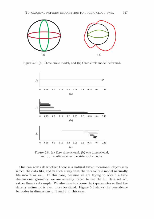
Topological pattern recognition for point cloud data 347
(a) (b)
Figure 5.5. (a) Three-circle model, and (b) three-circle model deformed.
(a)
(b)
(c)
β2
β1
β0
0 0.05 0.1 0.15 0.2 0.25 0.3 0.35 0.4 0.45
0 0.05 0.1 0.15 0.2 0.25 0.3 0.35 0.4 0.45
0 0.05 0.1 0.15 0.2 0.25 0.3 0.35 0.4 0.45
Figure 5.6. (a) Zero-dimensional, (b) one-dimensional,and (c) two-dimensional persistence barcodes.
One can now ask whether there is a natural two-dimensional object intowhich the data fits, and in such a way that the three-circle model naturallyfits into it as well. In this case, because we are trying to obtain a two-dimensional geometry, we are actually forced to use the full data set M,rather than a subsample. We also have to choose the k-parameter so that thedensity estimator is even more localized. Figure 5.6 shows the persistencebarcodes in dimensions 0, 1 and 2 in this case.

348 G. Carlsson
(a) (b)
Figure 5.7. (a) Torus and (b) Klein bottle.
P
PQ
Q
R
R
S
S
Figure 5.8. Identification space model for the Klein bottle.
Figure 5.6(a) suggests that the space is connected. Note that in the one-and two-dimensional barcodes (Figure 5.6(b,c)) there is an interval of signif-icant length (roughly from 0.15 to 0.30) in which there are two bars in theone-dimensional barcode and a single line in the two-dimensional barcode,suggesting that for that range of values of the scale parameter we have acomplex with β1 = 2 and β2 = 1, with F2 coefficients. There is a classifica-tion of all compact two-dimensional manifolds (Munkres 1975, Chapter 12),from which one can deduce that the only two possible such manifolds are thetorus and the Klein bottle, as in Figure 5.7. A calculation for the field F3
distinguishes between these two, and the persistent homology calculationsshows that the Klein bottle is the correct choice. The mod 3 Betti numbersof the torus are (1, 2, 1) and for the Klein bottle they are (1, 1, 0).
It is interesting to explore how the three-circle model might fit inside theKlein bottle. In order to do this, we will need a model of it more suitablefor computation. One way of doing this is via an identification space model,which can be pictured as in Figure 5.8. The points labelled P,Q,R, and S
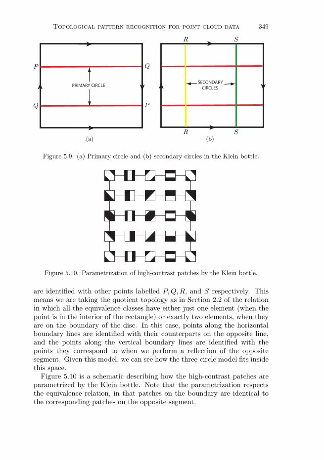
Topological pattern recognition for point cloud data 349
PRIMARY CIRCLE
P
P Q
Q
(a)
SECONDARY CIRCLES
R
R
S
S
(b)
Figure 5.9. (a) Primary circle and (b) secondary circles in the Klein bottle.
Figure 5.10. Parametrization of high-contrast patches by the Klein bottle.
are identified with other points labelled P,Q,R, and S respectively. Thismeans we are taking the quotient topology as in Section 2.2 of the relationin which all the equivalence classes have either just one element (when thepoint is in the interior of the rectangle) or exactly two elements, when theyare on the boundary of the disc. In this case, points along the horizontalboundary lines are identified with their counterparts on the opposite line,and the points along the vertical boundary lines are identified with thepoints they correspond to when we perform a reflection of the oppositesegment. Given this model, we can see how the three-circle model fits insidethis space.Figure 5.10 is a schematic describing how the high-contrast patches are
parametrized by the Klein bottle. Note that the parametrization respectsthe equivalence relation, in that patches on the boundary are identical tothe corresponding patches on the opposite segment.
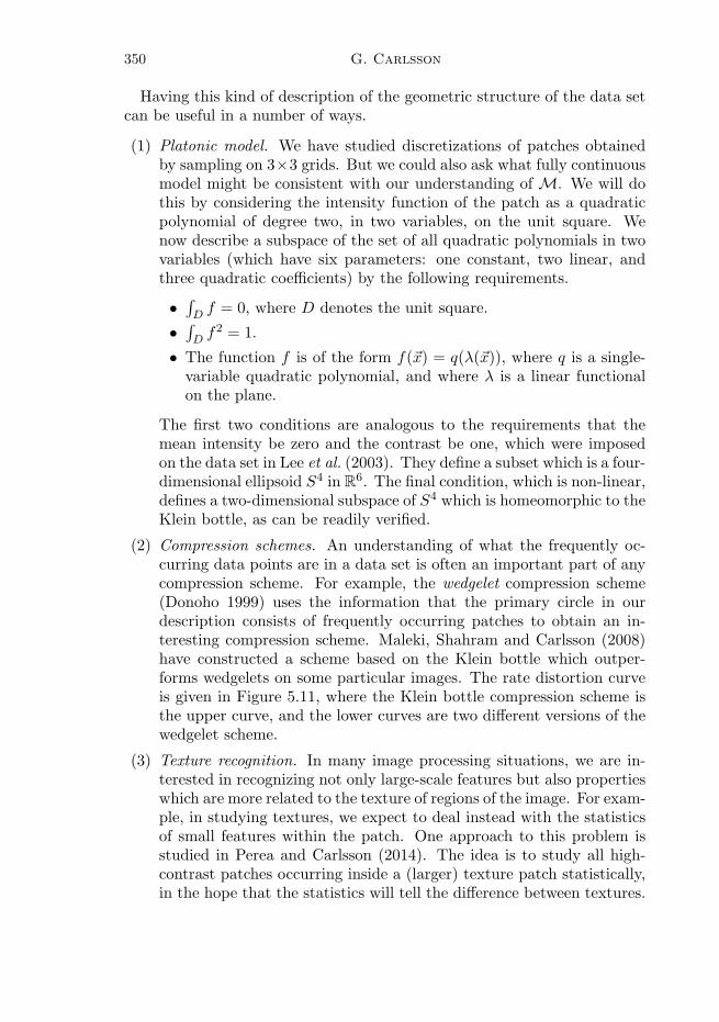
350 G. Carlsson
Having this kind of description of the geometric structure of the data setcan be useful in a number of ways.
(1) Platonic model. We have studied discretizations of patches obtainedby sampling on 3×3 grids. But we could also ask what fully continuousmodel might be consistent with our understanding of M. We will dothis by considering the intensity function of the patch as a quadraticpolynomial of degree two, in two variables, on the unit square. Wenow describe a subspace of the set of all quadratic polynomials in twovariables (which have six parameters: one constant, two linear, andthree quadratic coefficients) by the following requirements.
• ∫D f = 0, where D denotes the unit square.
• ∫D f2 = 1.
• The function f is of the form f(�x) = q(λ(�x)), where q is a single-variable quadratic polynomial, and where λ is a linear functionalon the plane.
The first two conditions are analogous to the requirements that themean intensity be zero and the contrast be one, which were imposedon the data set in Lee et al. (2003). They define a subset which is a four-dimensional ellipsoid S4 in R6. The final condition, which is non-linear,defines a two-dimensional subspace of S4 which is homeomorphic to theKlein bottle, as can be readily verified.
(2) Compression schemes. An understanding of what the frequently oc-curring data points are in a data set is often an important part of anycompression scheme. For example, the wedgelet compression scheme(Donoho 1999) uses the information that the primary circle in ourdescription consists of frequently occurring patches to obtain an in-teresting compression scheme. Maleki, Shahram and Carlsson (2008)have constructed a scheme based on the Klein bottle which outper-forms wedgelets on some particular images. The rate distortion curveis given in Figure 5.11, where the Klein bottle compression scheme isthe upper curve, and the lower curves are two different versions of thewedgelet scheme.
(3) Texture recognition. In many image processing situations, we are in-terested in recognizing not only large-scale features but also propertieswhich are more related to the texture of regions of the image. For exam-ple, in studying textures, we expect to deal instead with the statisticsof small features within the patch. One approach to this problem isstudied in Perea and Carlsson (2014). The idea is to study all high-contrast patches occurring inside a (larger) texture patch statistically,in the hope that the statistics will tell the difference between textures.

Topological pattern recognition for point cloud data 351
Adaptive Bi-WedgeletsAdaptive WedgeletsQuad Wedgelets
Adaptive Bi-WedgeletsAdaptive WedgeletsQuad Wedgelets
0 0.1 0.2 0.3 0.4 0.5 0.6 0.7 0.8 0.9 1.0
Bits per pixel (bpp)
25
24
23
22
21
20
19
18
17
16
PSN
R (d
B)
Figure 5.11. Rate distortion curve for Klein bottle-based compression.
One way to understand the statistics is to locate, for each high-contrastpatch, the closest point on the Klein bottle to that patch. If we carryout this process, we obtain a large collection of points on the Kleinbottle. We can then generate a probability density function on theKlein bottle by smoothing. Since the Klein bottle has a very simplegeometry (it has the torus as a two-fold covering space), we can per-form Fourier analysis on the probability density function, to obtaincoordinates which are the Fourier coefficients. It turns out that thesecoefficients are able to distinguish textures in various databases quiteeffectively, close to state of the art. The advantage of this method isthat the effect of rotation on an image gives an easy transformationon the Klein bottle, namely translation in the horizontal direction inthe identification space model in Figure 5.1. The standard approachto this problem is to identify a finite set of patches (the codebook),and to compute dot products of a given patch with each of them, giv-ing a distribution function on a finite set. The key observation here isthat we can deal with infinite codebooks if the codebook is equippedwith a useful geometry, as is the Klein bottle. Actual finiteness can bereplaced by finiteness of description.
5.2. Databases of compounds
In the previous section we saw that persistent homology can be a usefultool for understanding the overall structure of a complex data set. In thissection, we will discuss how persistence barcodes can instead be applied to

352 G. Carlsson
the individual elements, or data points, in databases where these elementsthemselves carry a geometric structure.Databases of organic compounds are of fundamental importance in many
biomedical applications. They are, for example, the main object of studyin the area of drug discovery. The possibility of developing methods for in-terrogating them, and in particular to determine rapidly and simply whichcompounds are functionally similar to which other compounds, is somethingthat should be explored. One approach to this problem is to somehow as-sign metric structures to sets of compounds. One difficulty is that sets ofcompounds do not fit neatly into standard formats for data, such as spread-sheets. The data specifying a particular compound consist of position coor-dinates for its atoms as well as information about bonds between the atoms.Since different compounds consist of different numbers of atoms as well asdifferent numbers of bonds, there is no simple vector description with a fixednumber of coordinates that can describe a set of compounds. In addition,the description is not unique, since a molecule could be rotated to producedifferent coordinates for the atoms. There is a standard method for encod-ing the structures of compounds, referred to as simplified molecular-inputline-entry system, or SMILES. In this system, the compounds are repre-sented as a list of symbols encoding the atoms, as well as other annotationsymbols which permit the reconstruction of the compound. Three problemswith this representation are that (a) there is not always a unique SMILESrepresentation of a given molecule, (b) the conversion from SMILES to athree-dimensional representation can be ambiguous, and (c) the structureis such that there is no obvious way of assigning a distance function or sim-ilarity score to a pair of SMILES structures. Bak and Lerner (2014) havedescribed a method for assigning distance functions to sets of compoundswhich circumvents these difficulties. We now describe their approach.Any compound can be described as a finite collection of atoms with po-
sitions in three-dimensional Euclidean space, together with a collection ofbonds connecting the atoms, and the lengths of the bonds. There are nowtwo ways to assign a metric space structure to the set of atoms.
(1) The three-dimensional Euclidean distance between atoms.
(2) By regarding the bonds as the edges in a weighted graph with theweight being the bond length, we may define an edge-path metric,where the distance between two atoms α and β is the minimum overall k and all sequences α0, α1, . . . , αk for which each pair (αi, αi+1) isconnected by a bond, of the sum
∑i
λ(αi, αi+1),
Topological pattern recognition for point cloud data 353
where λ(αi, αi+1) denotes the length of the bond connecting αi andαi+1.
A key observation concerning these metrics is that they are independent ofrotations of the molecules. Bak and Lerner (2014) have constructed variouspersistence barcodes, some using geometric constructions as in Section 3.6,and others using functional persistence (see Definition 3.18) based on variousfunctions on the set of atoms of the molecule. The geometric constructionsare of two types, namely the Vietoris–Rips complex constructed in Defini-tion 3.2 and the α complex defined in Section 3.6. The α complex is basedon the embedding of the set of atoms in three-dimensional Euclidean space.The fact that the atoms are embedded in a low-dimensional Euclidean spaceis what makes the α complex construction tractable. The collection of func-tions on the set of atoms used for the functional persistence barcodes is asfollows:
(1) the centrality function e2(x), defined in Section 3.5,
(2) the atomic mass of the atom,
(3) the partial charge of the atom.
In the case of functional persistence barcodes, a choice of scale must bemade. The choices made by Bak and Lerner (2014) are a finite set of smallmultiples of the carbon–carbon bond length within the molecule. Giventhese choices, persistence barcodes are now constructed in dimensions 0, 1,2 and 3. Let us index the set of choices of barcodes under considerationby β ∈ B, where B is an indexing set. Then, for each β, we assign thebottleneck distance or Wasserstein metric with p = 2, and label it dβ forthat particular complex construction. We can then assign an associatedweighted family of metrics
d�aB =
(∑β∈B
aβd2β
) 12
to any selection of non-negative real-valued vectors �a = {aβ}β .Bak and Lerner study a particular class of compounds called dihydro-
folate reductase (or DFHR) inhibitors. These are compounds that inhibitthe functioning of dihydrofolate reductase in the biosynthesis of purines,thymidylate, and other important amino acids. The synthesis which is asso-ciated with DFHR is important in the development of cancer, and thereforeinhibiting its functioning is a useful property in the management of cancer.DFHR inhibition is the basis for Methotrexate, which is the first histori-cal example of structure-based drug design applied to cancer. The idea inBak and Lerner (2014) is now to develop a database of drugs which mighthave some likelihood of being a DFHR inhibitor. To develop this database,they first observed that one necessary property of a DFHR inhibitor is
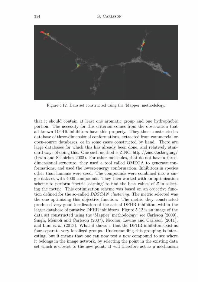
354 G. Carlsson
Figure 5.12. Data set constructed using the ‘Mapper’ methodology.
that it should contain at least one aromatic group and one hydrophobicportion. The necessity for this criterion comes from the observation thatall known DFHR inhibitors have this property. They then constructed adatabase of three-dimensional conformations, extracted from commercial oropen-source databases, or in some cases constructed by hand. There arelarge databases for which this has already been done, and relatively stan-dard ways of doing this. One such method is ZINC: http://zinc.docking.org/(Irwin and Schoichet 2005). For other molecules, that do not have a three-dimensional structure, they used a tool called OMEGA to generate con-formations, and used the lowest-energy conformation. Inhibitors in speciesother than humans were used. The compounds were combined into a sin-gle dataset with 4000 compounds. They then worked with an optimizationscheme to perform ‘metric learning’ to find the best values of �a in select-ing the metric. This optimization scheme was based on an objective func-tion defined for the so-called DBSCAN clustering. The metric selected wasthe one optimizing this objective function. The metric they constructedproduced very good localization of the actual DFHR inhibitors within thelarger database of putative DFHR inhibitors. Figure 5.12 is an image of thedata set constructed using the ‘Mapper’ methodology: see Carlsson (2009),Singh, Memoli and Carlsson (2007), Nicolau, Levine and Carlsson (2011),and Lum et al. (2013). What it shows is that the DFHR inhibitors exist asfour separate very localized groups. Understanding this grouping is inter-esting, but it means that one can now test a new compound to see whereit belongs in the image network, by selecting the point in the existing dataset which is closest to the new point. It will therefore act as a mechanism

Topological pattern recognition for point cloud data 355
for rejecting out of hand many compounds, which then do not have to betested in the laboratory.Bak and Lerner also used the algebraic functions defined in Section 4.2
to provide coordinates which can be used as input to more sophisticatedmachine learning methods. It was applied to the problem of classifyingDFHR inhibitor versus non-inhibitor status based only on the barcode.
5.3. Viral evolution
The phylogenetic tree has become the standard model to capture the evo-lution of species since Darwin. A single tree, the ‘Tree of Life’, containsall species, alive and extinct, into a single structure. The revolution in ge-nomic technologies in the last 20 years has led to an explosion of data andmethods developed to infer tree structure on sets of sequences (Felsenstein2004, Drummond, Nicholls, Rodrigo and Solomon 2002). This phylogeneticmodel strictly models clonal evolution, when genetic material is obtainedfrom a single lineage of ancestors. In this case mutations can occur and thenbe transmitted via replication of the genomic material from a single parentto the offspring. It is known that there are numerous other mechanismsfor the transfer of genetic material from one organism to another, wherethe organisms may even belong to different species. Recombination of ge-nomic material is common in many species. But examples across species arepervasive in nature, such as hybrids in plants, horizontal gene transfer inbacteria, and fusions of genomes, as occurred with mitochondria and chloro-plasts. It has been argued by Doolittle (1999) that trees do not adequatelymodel the full range of possible mechanisms for transfer of genetic material,thereby producing conflicting results in the reconstruction of the Tree ofLife. It turns out that all trees have vanishing homology groups, and thattherefore homological methods might be used to provide evidence for thepresence of horizontal evolutionary events within a collection of sequences,or in their genetic history. This idea was proposed by Chan, Carlsson andRabadan (2013), who outlined a dictionary of correspondences between al-gebraic topology and evolutionary concepts. The power of homology tostudy genomic data was shown with examples arising from viral evolution.The data sets consist of genetic sequences, which are sequences from
a four-element alphabet given by {A,G,C,T}, corresponding to the nu-cleotides adenine, guanine, cytosine, and thymine. One natural metric onthe set of such sequences is the Hamming distance, which assigns to a pairof sequences {xi}i and {yi}i, with xi, yi ∈ {A,G,C,T}, the number of val-ues of i for which xi = yi. Equivalently, one can describe the Hammingdistance as the minimal number of substitutions which have to be made inone sequence to obtain the other. There are many variants on this distancewhich take into account the rates at which the various substitutions take

356 G. Carlsson
place and assign different numbers to each possible substitution. Severalvariations of these distances were studied by Chan et al. (2013), with simi-lar results. The Nei–Tamura results were displayed. At this point we mayapply the persistent homology techniques to such finite metric spaces, andobtain persistence barcodes.Since what we are trying to do is to distinguish some of these metric
spaces from trees, it is important to understand the behaviour of persistenthomology of spaces which are somehow ‘tree-like’. Let Γ denote a weightedgraph, that is, a triple (V (Γ), E(Γ), fΓ), where V (Γ) is a finite set, E(Γ)is a subset of the collection of two-element subsets of V (Γ), and wherefΓ : E(Γ)→ (0,+∞) is a weighting function on the edges. By an edge-pathin Γ, we will mean a sequence {v0, v1, . . . , vn} of elements vi ∈ V (Γ) suchthat for every 0 ≤ i ≤ n− 1, we have that {vi, vi+1} is an element of E(Γ).For any edge path e = {v0, v1, . . . , vn}, the length of e, denoted by λ(e), isgiven by
λ(e) =n−1∑i=0
fΓ({vi, vi+1}).
The distance between any two vertices v and v′ of Γ, dΓ(v, v′), is given by
dΓ(v, v′) = min
eλ(e),
where the minimum is taken over all edge-paths e = {v0, . . . , vn} with theproperty that v0 = v and vn = v′. We denote the metric space (V (Γ), dΓ) byM(Γ). We now have the following result concerning the positive-dimensionalpersistent barcodes of a metric space M(Γ).
Proposition 5.1. Let Γ be any weighted graph, and assume that theunderlying undirected graph is a tree, that is, it admits no cycles. Then thepersistence barcodes βi(M(Γ)) are all trivial, that is, they are the emptymultiset of bars, whenever i > 0.
Remark 5.2. This result uses in an essential way the result proved byBuneman (1974) that a metric space is of the form M(Γ) if and only if itsatisfies the so-called four-point condition, which asserts that a finite metricspace (X, d) is of the form M(Γ) for some weighted tree if and only if thecondition
d(x, y) + d(z, t) ≤ max(d(x, z) + d(y, t), d(x, t) + d(y, z))
holds for all quadruples of elements x, y, z, t ∈ X.
The effect of this result is that one can determine that a finite metricspace is not tree-like, or is isometric to a finite subset of a space of the formM(Γ). This statement alone is not useful in studying data, since there will
Topological pattern recognition for point cloud data 357
be no ‘exactly tree-like’ metric spaces occurring in the presence of noise.However, we have Theorem 4.2, which shows us that if a finite metric spaceis approximately a tree-like metric space, that is, close to a tree-like metricspace in the Gromov–Hausdorff metric, then its higher-dimensional barcodeswill be close to the empty barcode in the bottleneck distance. This meansthat all the intervals contained in the barcode are of small length.Chan et al. (2013) applied persistent homology in one and two dimensions
to data sets arising in viral evolution, using the Vietoris–Rips and witnesscomplex defined in Section 3.6. A summary of their results is as follows (seeChan et al. 2013 for details).
(1) The type of exchange of genomic material can be catalogued by thetopology of the genomic data. In the case of strict clonal evolution,all information is captured by the zero-dimensional homology. Seg-mented viruses, that is, viruses whose genomic information is encodedin different ‘chromosomes’ or segments, undergo reassortments: thegeneration of novel viruses with combinations of segments from thedifferent parental strains. This phenomenon is the source of most ofthe reported influenza pandemics in humans (the H2N2 pandemic in1957 and H3N2 in 1968), where a novel viral strain is generated by reas-sorting segments of different parental strains infecting different hosts.A data set of sequences arising in avian influenza was studied fromthis point of view. When each distinct segment was studied, therewas no higher-dimensional behaviour. However, the metric space pro-duced by using the concatenated sequences did produce significant one-dimensional homology, which would preclude phylogeny as a completeexplanation. Other viruses, such as HIV, the cause of AIDS, undergorecombination, where the genome of the offspring is a mosaic of thegenome of the parents. Circulating recombinant forms (CRFs) are ex-amples of HIV viruses with complex recombinant patterns. Persistenthomology shows higher-dimensional homology groups capturing someof the complex recombinant structures.
(2) Estimating the rate and scale of horizontal evolution. By performingpersistent homological calculations on simulations, it was observed thata lower bound for the recombination/reassortment rate was obtainedby studying the counts of the number of bars in the correspondingbarcode. By analysing the numbers of these events it was possible toassess the evolutionary pressures that link different pieces of genomicmaterial together. For instance, when analysing the homology of avianinfluenza A, it was shown that several segments, containing the genesthat encode the polymerases, are more likely to co-segregate together,possibly indicating that natural selection does not allow all combina-tions to be equally fit.

358 G. Carlsson
(3) Higher-dimensional homology generators capture genomic exchange.In cases where higher-dimensional homology was observed, a repre-sentative cycle for a given feature (or bar) was obtained. Such a cy-cle is a linear combination of pairs of landmark points in the case ofone-dimensional homology, of triples of landmark points in the caseof two-dimensional homology, and so on. The cycle then gives a listof data points which occur, and this list was studied. In the casesstudied, these occurrences were consistent with the known horizontaltransfer mechanisms in these situations. It should be pointed out thatthe representative cycle was chosen directly from the algorithms usedto compute the persistent homology, and no effort was made to find theminimal cycle, that is, one with the smallest number of summands inthe formal sum. Choosing the minimal cycle would be expected to giveeven more focused outcomes. One might also attempt to reconcile thefindings of homology with results obtained via the mapping methodsintroduced in Singh et al. (2007).
(4) Explicit examples were studied: the triple reassortant avian virus thatled to the outbreak in China in March 2013, the rate of reassortmentof influenza A viruses infecting different hosts (humans, swine andbirds), HIV recombination, and many other viruses including denguevirus, hepatitis C virus, West Nile virus, and rabies.
5.4. Time series
Time series are a very interesting class of data, where for a discrete variablet we have a point xt in a metric space (X, d). Usually X is a Euclidean spaceRn. Given such a time series and a positive integer l, we can construct adata set out of the time series {xt}t as follows. Let Tl({xt}t) denote theset of all fragments (xti , xti+1 , . . . , xti+l
) for every possible initial time ti.From the distance function d on X, we can define a distance function dT onTl({xt}t) by the formula
dT ((xti , xti+1 , . . . , xti+l), (xtj , xtj+1 , . . . , xtj+l
)) =
( s=l∑s=0
d(xti+s, xtj+s)2
) 12
.
To give an idea of how this works, we consider a time series given by
xt = sin(tε),
where ε > 0 is a very small number, or threshold. If l = 0, then the dataset we obtain is just the range of the sine function restricted to the set ofmultiples of the threshold ε. If ε is sufficiently small, it will roughly fill outthe interval [−1, 1], the range of the sine function. On the other hand, ifl = 1, then the data points are pairs (sin(tε), sin((t+1)ε)). A sketch of thisdata set in the case where ε = π/4 is shown in Figure 5.13. It is easy to

Topological pattern recognition for point cloud data 359
Figure 5.13. A space of time series fragments.
check, using trigonometric identities, that this set is a discrete set of pointslying on the ellipse
x2 −√2
2xy + y2 =
1
2.
The fact that this data set contains a loop reflects the fact that the sinefunction is periodic. If we performed the same construction for a time seriesof the form xt = tε, we would instead obtain a set of points sampled fromthe line with equation y = x + ε. This set has no loops, and this reflectsthe fact that the linear function f(x) = xε is not periodic. These observa-tions suggest the possibility that computing the one-dimensional persistenthomology groups of the metric spaces Tl({xt}t) could be a strategy for de-tecting periodic behaviour of a given function. This method is proposedby Perea and Harer (2014), and some of its properties are explored. Wesummarize their results below.For any real-valued function f on the real line, we will define the sliding
window embedding attached to f and with parameters M ∈ N and τ ∈(0,+∞), denoted by SWM,τf(t), by
SWM,τf(t) = (f(t), f(t+ τ), . . . , f(t+Mτ)),
where SWM.τf is an RM+1-valued function on R. By choosing a finite setof points T ∈ [0, L], we obtain a point cloud attached to the function f ,which we denote by C = C(f,M, τ, T ). It is the persistent homology ofC, using the Vietoris–Rips complex, which will reflect periodic behaviour.To formulate the main result of Perea and Harer (2014), we make somedefinitions. For any L2 function on the circle S1, we let Snf denote its NthFourier truncation, that is, the linear combinations of sin(nt) and cos(nt),for n ≤ N , occurring in the Fourier decomposition for f . For any finiteset T ⊆ S1, we can then apply the sliding window embedding for SNf ,
360 G. Carlsson
based on M and τ , and restrict it to T , to obtain a point cloud in (M +1)-dimensional Euclidean space Y = Y (f, T,N,M, τ). We then apply a processwhich mean-centres every data point in Y , and then normalizes it to lie onthe unit sphere in RM+1. That is, for each data point x = (x0, x1, . . . , xM ),we first transform it to a vector x = (x0, x1, . . . , xn), where
xi = xi − 1
M + 1
(∑i
xi
).
Finally, we form x∗ = x/‖x‖. We will denote the point cloud which has beentransformed in this way by Y (f, T,N,M, τ). We next assume the functionf is L-periodic on R, so that
f
(x+
2π
L
)= f(x).
We then set
τN =2π
L(2N + 1).
It is then shown in Perea and Harer (2014) that the limit of the sequencedgmY (f, T,N, 2N, τN ) exists as a point dgm∞(f, T, w) in the completed
barcode space B∞, based on the bottleneck distance, defined in Section 4.4,where dgm denotes the operation which assigns to a point cloud its one-dimensional persistence diagram, or barcode, and where w = 2π/L. Forany barcode β = {(x1, y1), . . . , (xn, yn)} in B∞, we define its maximal per-sistence mp(β) by the equation mp(β) = maxi(yi − xi). It is easy to check
that mp extends to a function on B∞. Perea and Harer (2014) have alsoproved that one may take a limit over families of subsets Tδ ⊆ S1, where Tδ
is δ-dense in the sense that every point in S1 is within a distance δ of somepoint in Tδ, and where δ → 0, to obtain a limit dgm∞(f, w). One of theprincipal results of Perea and Harer (2014) is as follows.
Theorem 5.3. Let f be an L-periodic continuous function on S1 suchthat f(0) = 0 and ‖f‖2 = 1, and suppose that the persistence diagram iscomputed for homology with coefficients in Q. Then we have that
mp(dgm∞(f, w)) ≥ 2√2max
n∈N|f(n)|,
where f(n) is given by f(n) = 12an − i
2bn if n > 0, = 12a−n +
i2b−n is n < 0,
and = a0 if n = 0, where an and bn denote the coefficients of cos(nt) andsin(nt), respectively, in the Fourier expansion of f .
This is a very interesting relationship, and these observations are usedas the basis for a test for periodicity based on persistence barcodes of thepoint clouds constructed from the function f . Perea and Harer (2014) made
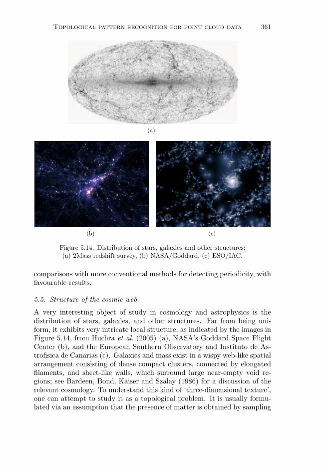
Topological pattern recognition for point cloud data 361
(a)
(b) (c)
Figure 5.14. Distribution of stars, galaxies and other structures:(a) 2Mass redshift survey, (b) NASA/Goddard, (c) ESO/IAC.
comparisons with more conventional methods for detecting periodicity, withfavourable results.
5.5. Structure of the cosmic web
A very interesting object of study in cosmology and astrophysics is thedistribution of stars, galaxies, and other structures. Far from being uni-form, it exhibits very intricate local structure, as indicated by the images inFigure 5.14, from Huchra et al. (2005) (a), NASA’s Goddard Space FlightCenter (b), and the European Southern Observatory and Instituto de As-trofisica de Canarias (c). Galaxies and mass exist in a wispy web-like spatialarrangement consisting of dense compact clusters, connected by elongatedfilaments, and sheet-like walls, which surround large near-empty void re-gions; see Bardeen, Bond, Kaiser and Szalay (1986) for a discussion of therelevant cosmology. To understand this kind of ‘three-dimensional texture’,one can attempt to study it as a topological problem. It is usually formu-lated via an assumption that the presence of matter is obtained by sampling

362 G. Carlsson
from a density function ρ defined on three-dimensional space. The densityρ would itself be a complicated object, given the complexity of the resultingsampling. The first recognition that topological methods could be usefulin this setting occurred in Gott, Dickinson and Melott (1986) and Hamil-ton, Gott and Weinberg (1986). The idea was that one should study thelevel sets of ρ from a topological point of view. These level sets are two-dimensional surfaces, for which there is a natural integer invariant calledthe genus, which is defined as one half of its first Betti number. Gott et al.(1986) and Hamilton et al. (1986) considered the genus of the level surfacesas a useful numerical invariant of this situation. Note that the genus differsfrom the Euler characteristic, defined below, by a constant. Another familyof spaces one could study is the excursion sets at various levels r, defined asρ−1([r,+∞)). It was recognized in Sousbie (2011) and Sousbie, Pichon andKawahara (2011) that persistent homology gives a method which allows usto track topological behaviour of excursion sets as the thresholds for theseexcursion sets decrease.In order to develop theory, and to understand the appearance of observed
results, one can assume that ρ is itself a random function, or a random field,obtained under some stochastic process. The idea is that one could attemptto understand expected values for the Betti numbers of the excursion setsof random fields. Random fields have been studied in great detail in Adler(1981) and Adler and Taylor (2007). A case of particular interest is that ofa Gaussian random field, in which the assumption is made that the distri-bution assumed by the values of the random field at any particular point orany finite family of points in the domain is Gaussian. Gaussian fields in acosmological context are of key importance because of the following facts.
(1) The primordial universe was, to high precision, a spatial Gaussianrandom field, which has been shown observationally by numerous cos-mic microwave background experiments such as COBE (Bennett et al.2003), WMAP (Spergel et al. 2007), and more recently Planck (Abergelet al. 2011).
(2) There is also a fundamental physical reason to expect that all primor-dial structure is nearly completely Gaussian. This concerns the gener-ation of primordial density perturbations during the early inflationaryphase of the universe (at t ∼ 10−36 seconds after the Big Bang), duringwhich quantum fluctuations were blown up to macroscopic proportions.
(3) A more technical mathematical reason why Gaussian fluctuations areexpected is the central limit theorem. Given the fact that the fluctu-ations at each scale are independently distributed, it would naturallygive rise to a Gaussian field.
This assumption permits us to understand many properties of the randomfield, including some topological ones.

Topological pattern recognition for point cloud data 363
There is another useful integer-valued summary of the homology of anyfinite-dimensional space called the Euler characteristic of the space. It isdefined to be the alternating sum
χ(X) =∑i
(−1)iβi(X).
Note that there is an Euler characteristic for each different field of coeffi-cients. The Euler characteristic is a very useful invariant due to the factthat it is so readily computable, as is demonstrated in the following result.
Proposition 5.4. Let X be any finite simplicial complex. Then χ(X) isequal to the alternating sum ∑
i
(−1)iσi(X),
where σi(X) denotes the number of i-dimensional simplices in the com-plex X.
What this means is that the Euler characteristic can be computed directlyby counting simplices, without performing any linear algebra. The price onepays is, of course, that much information about the actual homology is lost.
Example 5.5. Let Sn denote the n-sphere. Then χ(Sn) = 0 if n is odd,and 2 if n is even. So, while the Betti numbers can distinguish betweenall spheres, the Euler characteristic can only determine the parity of thedimension of the sphere.
It turns out that for many Gaussian random fields, as shown by Adler andTaylor, it is possible to determine the distribution of the statistic given bythe Euler characteristic of the excursion sets, in terms of certain parametersdefining the random field. These beautiful results are described in detail inAdler and Taylor (2007). An important case (when the Gaussian field ischaracterized by its power spectrum) was obtained in the cosmological liter-ature (Bardeen et al. 1986, Hamilton et al. 1986). What this suggests is thepossibility that we can begin to evaluate models for the stochastic processesfrom which the distribution in the cosmic web is generated, provided thatwe can develop sufficient theory to do so.More recently, Park et al. (2013) and van de Weygaert et al. (2011) have
shown that the Betti numbers of Gaussian random fields carry strictly moreinformation concerning the random field than the Euler characteristic alone.Specifically, it is found that an invariant of the Gaussian field called theslope of the power spectrum affects the shape of the curves of the Bettinumbers (as the threshold r changes), while the shape of the curve of Eulercharacteristics is independent of it.

364 G. Carlsson
Persistent homology has also been studied in this way. Adler et al. (2010)have defined the analogue of the Euler characteristic for persistent homologyand studied it for Gaussian random fields. The analogue of the Euler char-acteristic for persistent homology is defined as follows. For a fixed barcodeβ = {(x1, y1), . . . , (xn, yn)}, we define
τ(β) =∑i
(yi − xi),
and then define the analogue of the Euler characteristic, χpers by the formula
χpers(X) =∑i
(−1)iτ(βi(X)),
where βi(X) denotes the i-dimensional persistence barcode for X. Thisquantity has the same properties which make the Euler characteristic highlycomputable, and in Adler et al. (2010) a result is proved which computesχpers for Gaussian random fields.Finally, van de Weygaert et al. (2011) have taken a different topological
approach to analyse the topology at various scales of a set of discrete pointsin two- or three-dimensional space. The points are to be thought of as indi-vidual stars, or perhaps galaxies, and the idea is to construct the α complex(see Section 3.6) associated to them at various scales. This method is usedby van de Weygaert et al. (2011) to study the Betti numbers produced byvarious stochastic process models, including some which are explicitly pro-posed for cosmological problems. In addition, they point out that persistenthomology is applicable to this family of complexes, and will likely be appliedin future investigations.
Acknowledgements
The author is very grateful for helpful conversations with many people, in-cluding R. Adler, A. Bak, A. Blumberg, E. Carlsson, J. Carlsson, F. Chazal,J. Curry, V. de Silva, P. Diaconis, H. Edelsbrunner, R. Ghrist, L. Guibas,J. Harer, S. Holmes, M. Lesnick, A. Levine, P. Lum, B. Mann, F. Memoli,K. Mischaikow, D. Morozov, S. Mukherjee, J. Perea, R. Rabadan, H. Sex-ton, P. Skraba, G. Singh, R. van de Weijgaert, M. Vejdemo-Johansson,S. Weinberger, and A. Zomorodian.

Topological pattern recognition for point cloud data 365
REFERENCES1
A. Abergel et al. (2011), ‘Planck early results XXIV: Dust in the diffuse interstellarmedium and the galactic halo’, Astron. Astrophys. 536, A24.
R. Adler (1981), The Geometry of Random Fields, Wiley Series in Probability andMathematical Statistics.
R. Adler and J. Taylor (2007), Random Fields and Geometry, Springer Monographsin Mathematics.
R. Adler, O. Bobrowski, M. Borman, E. Subag and S. Weinberger (2010), Persistenthomology for random fields and complexes. In Borrowing Strength: TheoryPowering Applications: A Festschrift for Lawrence D. Brown, Vol. 6, pp. 124–143.
A. Bak and M. Lerner (2014), in preparation.J. Bardeen, J. Bond, N. Kaiser and A. Szalay (1986), ‘The statistics of peaks of
Gaussian random fields’, Astrophys. J. 304, 15–61.C. Bennett, R. Hill, G. Hinshaw, M. Nolta, N. Odegard, L. Page, D. Spergel, J. Wei-
land, E. Wright, M. Halpern, N. Jarosik, A. Kogut, M. Limon, S. Meyer, G.Tucker and E. Wollack (2003), ‘First-year Wilkinson Microwave AnisotropyProbe (WMAP)* observations: Foreground emission’, Astrophys. J. Supple-ment Series 148, 97.
A. Blumberg, I. Gal, M. Mandell and M. Pancia (2013), Robust statistics, hy-pothesis testing, and confidence intervals for persistent homology on metricmeasure spaces. arXiv:1206.4581
O. Bonnet (1848), ‘Memoire sur la theorie generale des surfaces’, Journal de l’EcolePolytechnique 19, 1–146.
P. Buneman (1974), ‘A note on the metric properties of trees’, J. Combin. TheoryB 17, 48–50.
D. Burago, Y. Burago and S. Ivanov (2001), A Course in Metric Geometry, Vol. 33of Graduate Studies in Mathematics, AMS.
G. Carlsson (2009), ‘Topology and data’, Bull. Amer. Math. Soc. 46, 255–308.G. Carlsson and V. de Silva (2010), ‘Zigzag persistence’, Found. Comput. Math.
10, 367–405.G. Carlsson and A. Zomorodian (2009), ‘The theory of multidimensional persis-
tence’, Discrete Comput. Geom. 42, 71–93.G. Carlsson, T. Ishkhanov, V. de Silva and A. Zomorodian (2008), ‘On the local
behavior of spaces of natural images’, Internat. J. Computer Vision 76, 1–12.G. Carlsson, V. de Silva and D. Morozov (2009), Zigzag persistent homology and
real-valued functions. In Proc. 25th Annual Symposium on ComputationalGeometry, ACM, pp. 247–256.
G. Carlsson, A. Zomorodian, A. Collins and L. Guibas (2005), ‘Persistence barcodesfor shapes’, Internat. J. Shape Modeling 11, 149.
J. Chan, G. Carlsson and R. Rabadan (2013), ‘Topology of viral evolution’, Proc.Nat. Acad. Sci. 110, 18566–18571.
1 The URLs cited in this work were correct at the time of going to press, but the publisherand the authors make no undertaking that the citations remain live or are accurate orappropriate.

366 G. Carlsson
F. Chazal, D. Cohen-Steiner, L. Guibas, F. Memoli and S. Oudot (2009), Gromov–Hausdorff stable signatures for shapes using persistence. In Eurographics Sym-posium on Geometry Processing 2009. Computer Graphics Forum 28, 1393–1403.
F. Chazal, D. Cohen-Steiner and Q. Merigot (2011), ‘Geometric inference for prob-ability measures’, Found. Comput. Math. 11, 733–751.
D. Cohen-Steiner, H. Edelsbrunner and J. Harer (2007), ‘Stability of persistencediagrams’, Discrete Comput. Geom. 37, 103–120.
D. Cohen-Steiner, H. Edelsbrunner, J. Harer and Y. Mileyko (2010), ‘Lipschitzfunctions have Lp-stable persistence’, Found. Comput. Math. 10, 127–139.
J. Dalbec (1999), ‘Multisymmetric functions’, Beitrage Algebra Geom. 40, 27–51H. Derksen and J. Weyman (2005), ‘Quiver representations’, Notices Amer. Math.
Soc. 52, 200–206.D. Donoho (1999), ‘Wedgelets: Nearly minimax estimation of edges’, Ann. Statist.
27, 859–897.W. Doolittle (1999), ‘Phylogenetic classification and the universal tree’, Science
284 (5423), 2124–2128.A. Drummond, F. Nicholls, A. Rodrigo and W. Solomon (2002), ‘Estimating mu-
tation parameters, population history, and genealogy simultaneously fromtemporally spaced sequence data’, Genetics 161, 1307–1320.
H. Edelsbrunner, D. Letscher and A. Zomorodian (2002), ‘Topological persistenceand simplification’, Discrete Comput. Geom. 28, 511–533
S. Eilenberg (1944), ‘Singular homology theory’, Ann. of Math. 45, 407–447.L. Euler (1741), ‘Solutio problematis ad geometriam situs pertinentis’, Commen-
tarii Academiae Scientiarum Petropolitanae 8, 128–140.L. Euler (1758a), ‘Elementa doctrinae solidorum’, Novi Commentarii Academiae
Scientiarum Petropolitanae 4, 109–140. Opera Omnia (1) 26, 72–93.L. Euler (1758b), ‘Demonstratio nonnullarum insignium proprietatum quibus sol-
ida hedris planis inclusa sunt praedita’, Novi Commentarii Academiae Scien-tiarum Petropolitanae 4, 140–160. Opera Omnia (1) 26, 94–108.
J. Felsenstein (2004), Inferring Phylogenies, Sinauer Associates, Sunderland, MA.M. Frechet (1944), ‘L’integrale abstraite d’une fonction abstraite d’une variable
abstraite et son application a la moyenne d’un element aleatoire de naturequelconque’ Rev. Sci. 82, 483–512.
M. Frechet (1948), ‘Les elements aleatoires de nature quelconque dans un espacedistancie’ Ann. Inst. Henri Poincare 10, 215–310.
P. Gabriel (1972), ‘Unzerlegbare Darstellungen I’, Manuscr. Math. 6, 71–103.A. Greven, P. Pfaffelhuber and A. Winter (2009), ‘Convergence in distribution of
random metric measure spaces’, Probab. Theory Rel. Fields 145, 285–322.J. Gott, M. Dickinson and A. Melott (1986), ‘The sponge-like topology of large-
scale structure in the universe’, Astrophys. J. 306, 341–357.A. Hamilton, J. Gott and D. Weinberg (1986), ‘The topology of the large-scale
structure of the universe’, Astrophys. J. 309, 1–12.J. Hartigan (1975), Clustering Algorithms, Wiley Series in Probability and Math-
ematical Statistics.A. Hatcher (2002), Algebraic Topology, Cambridge University Press.
Topological pattern recognition for point cloud data 367
J. van Hateren and A. van der Schaaf (1998), ‘Independent component filters ofnatural images compared with simple cells in primary visual cortex’, Proc. R.Soc. Lond. B 265, 359–366.
J. Huchra, T. Jarrett, M. Skrutskie, R. Cutri, S. Schneider and L. Macri (2005),The 2MASS redshift survey and low galactic latitude large-scale structure. InNearby Large-Scale Structures and the Zone of Avoidance (K. P. Fairall andP. A. Woudt, eds), ASP Conference Series, Vol. 329.
J. Irwin and B. Schoichet (2005), ‘ZINC: A free database of commercially availablecompounds for virtual screening’, J. Chem. Inf. Model. 45, 177–182.
H. Karcher (1977), ‘Riemannian center of mass and mollifier smoothing’, Comm.Pure Appl. Math. 30, 509–541.
W. Kendall (1990), ‘Probability, convexity, and harmonic maps with small image I:Uniqueness and fine existence’, Proc. London Math. Soc. 61, 371–406.
J. Kogan (2007), Introduction to Clustering Large and High-Dimensional Data,Cambridge University Press.
A. Lee, K. Pedersen and D. Mumford (2003), ‘The non-linear statistics of highcontrast patches in natural images’, Internat. J. Computer Vision 54, 83–103.
D. Lipsky, P. Skraba and M. Vejdemo-Johansson (2011), A spectral sequence forparallelized persistence. arXiv:1112.1245
J. Listing (1848), Vorstudien zur Topologie, Vandenhoeck und Ruprecht.P. Lum, G. Singh, J. Carlsson, A. Lehman, T. Ishkhanov, M. Vejdemo-Johansson,
M. Alagappan and G. Carlsson (2013), Extracting insights from the shape ofcomplex data using topology. Nature Scientific Reports 3, # 1236.
S. Mac Lane (1998), Categories for the Working Mathematician, second edition,Vol. 5 of Graduate Texts in Mathematics, Springer.
A. Maleki, M. Shahram and G. Carlsson (2008), Near optimal coder for imagegeometries. In Proc. 15th IEEE International Conference on Image Processing(ICIP), pp. 1061–1064.
Y. Mileyko, S. Mukherjee and J. Harer (2011), ‘Probability measures on the spaceof persistence diagrams’, Inverse Problems 27, 1–22.
J. Milnor (1963), Morse Theory, Princeton University Press.J. Munkres (1975), Topology: A First Course, Prentice Hall.M. Nicolau, A. Levine and G. Carlsson (2011), Topology based data analysis identi-
fies a subgroup of breast cancers with a unique mutational profile and excellentsurvival. Proc. Nat. Acad. Sci. 108, 7265–7270.
P. Niyogi, S. Smale and S. Weinberger (2008), ‘Finding the homology of subman-ifolds with high confidence from random samples’, Discrete Comput. Geom.39, 419–441.
C. Park, P. Pranav, P. Chingangram, R. van de Weygaert, B. Jones, G. Vegter,I. Kim, J. Hidding and W. Helwing (2013), ‘Betti numbers of Gaussian fields’,J. Korean Astron. Soc. 46, 125–131.
J. Perea and G. Carlsson (2014), ‘A Klein bottle-based dictionary for texture rep-resentation’, Internat. J. Computer Vision 107, 75–97.
J. Perea and J. Harer (2014), Sliding windows and persistence: An application oftopological methods to signal analysis. arXiv:1307.6188v1
H. Poincare (1895), ‘Analysis situs’, Journal de l’Ecole Polytechnique (2) 1, 1–123.

368 G. Carlsson
B. Riemann (1851), Grundlagen fur eine allgemeine Theorie der Functionen einerveranderlichen complexen Grosse. Dissertation, Gottingen.
V. Robins (1999), ‘Towards computing homology from finite approximations’,Topology Proceedings 24 (1), 503–532.
G. Segal (1968), ‘Classifying spaces and spectral sequences’, Inst. Hautes EtudesSci. Publ. Math. 34, 105–112.
V. de Silva and G. Carlsson (2004), Topological estimation using witness complexes.In Proc. First Eurographics Conference on Point-Based Graphics, pp. 157–166.
G. Singh, F. Memoli and G. Carlsson (2007), Topological methods for the analysisof high dimensional data sets and 3D object recognition. In Proc. EurographicsSymposium on Point-Based Graphics 2007 (M. Botsch and R. Pajarola, eds).
T. Sousbie (2011), ‘The persistent cosmic web and its filamentary structure I:Theory and implementation’, Mon. Not. R. Astron. Soc. 414, 350–383.
T. Sousbie, C. Pichon and H. Kawahara (2011), ‘The persistent cosmic web andits filamentary structure II: Illustrations’, Mon. Not. R. Astron. Soc. 414,384–403.
D. Spergel, R. Bean, O. Dore, M. Nolta, C. Bennett, J. Dunkley, G. Hinshaw,N. Jarosik, E. Komatsu, L. Page, H. Peiris, L. Verde, M. Halpern, R.Hill, A. Kogut, M. Limon, S. S. Meyer, N. Odegards, G. Tucker, J. Wei-land, E. Wollack and E. Wright (2007) ‘Three-year Wilkinson MicrowaveAnisotropy Probe (WMAP) observations: Implications for cosmology’, As-trophys. J. Supplement Series 170, 377–408.
K. Turner, Y. Mileyko, S. Mukherjee and J. Harer (2014), Frechet means for dis-tributions of persistence diagrams. arXiv:1206.2790v2
A. Vandermonde (1774), Remarques sur les problemes de situation. In Memoiresde l’Academie Royale des Sciences pour 1771, Paris, pp. 556–574.
R. van de Weygaert, G. Vegter, H. Edelsbrunner, B. Jones, P. Pranav, C. Park,W. Hellwing, B. Eldering, N. Kruithof, E. Bos, J. Hidding, J. Feldbrugge,E. ten Have, M. van Engelen, M. Caroli and M. Teillaud (2011), Alpha,Betti, and the Megaparsec Universe: On the topology of the cosmic web. InTransactions on Computational Science XIV (M. L. Gavrilova et al., eds),Vol. 6970 of Lecture Notes in Computer Science, Springer, pp. 60–101.
A. Zomorodian (2005), Topology for Computing, Vol. 16 of Cambridge Monographson Applied and Computational Mathematics, Cambridge University Press.
A. Zomorodian (2010), The tidy set: A minimal simplicial set for computing homol-ogy of clique complexes. In Proc. 2010 Annual Symposium on ComputationalGeometry, ACM, pp. 257–266.
A. Zomorodian and G. Carlsson (2005), ‘Computing persistent homology’, DiscreteComput. Geom. 33, 247–274.