Embed Size (px)
Citation preview
UNIVERSIDADE DE SÃO PAULO
INSTITUTO DE FÍSICA DE SÃO CARLOS
MARIANE BARSI ANDREETA
Topological study of reservoir rocks and acidification processes using
complex networks methods
SÃO CARLOS
2017


MARIANE BARSI ANDREETA
Topological study of reservoir rocks and acidification processes using
complex networks methods
Thesis presented to the Graduate Program in Physics at the Instituto de Física de São Carlos, Universidade de São Paulo to obtain the degree of Doctor of Science. Concentration area: Applied Physics Option: Computational Physics Advisor:Prof. Dr. Tito José Bonagamba
Corrected Version (Original version available on the Program Unit)
SÃO CARLOS
2017

I AUTHORIZE THE REPRODUCTION AND DISSEMINATION OF TOTAL ORPARTIAL COPIES OF THIS DOCUMENT, BY CONVENCIONAL OR ELECTRONICMEDIA FOR STUDY OR RESEARCH PURPOSE, SINCE IT IS REFERENCED.
Cataloguing data revised by the Library and Information Service of the IFSC, with information provided by the author
Andreeta, Mariane Barsi Topological study of reservoir rocks andacidification processes using complex networksmethods / Mariane Barsi Andreeta; advisor Tito JoséBonagamba - revised version -- São Carlos 2017. 117 p.
Thesis (Doctorate - Graduate Program inComputational Physics) -- Instituto de Física de SãoCarlos, Universidade de São Paulo - Brasil , 2017.
1. Digital rock. 2. Petrophysics. 3. Porenetworks. 4. Complex networks. 5. Wormhole. I.Bonagamba, Tito José, advisor. II. Title.

To my beloved parents.


ACKNOWLEDGEMENTS
This work is the result of the collaboration of many people, without them, could never
been accomplished.
I’d like to express my deepest gratitude to my advisor, professor Tito José Bonagamba,
for his courage to delve into new frontiers of knowledge, for his trust in me and support
throughout this endeavor.
My gratitude to my colleague and friend, Everton Lucas de Oliveira, for the insights,
discussions and for the friendship. Without our talks none of this work would be possible.
To professor Francisco Aparecido Rodrigues, that gave me the first stepping stones into
the world of networks.
To our collaborators, Carlos Speglich – Cenpes/Petrobras and Roberson Saraiva Polli -
UNIFESP, that presented me with the challenges of the industry on the acidification front,
trusted my work and provided the samples used in this project.
To the LEAR family: Aparecido Donizeti Fernandes de Amorim, Dr. Edson Vidoto,
Arthur Ferreira de Araújo, Daniel Jardon, Elton Tadeu Montrazi, Everton Lucas de Oliveira,
Rodrigo Silva de Oliveira; and the newly acquired members Marta Jacomo, Bernd Foester,
Alessandro Sá. Thank you for the support, discussions.and friendship.
To my friends: Rejane, Filipi, Celso, Ila, Alex, Issao, Leonardo. You guys make my days
much happier, thank you! Thank you for being part of my life, and for being there when
times were difficult.
To my brothers and sisters in family, Marcello and Erika, Marcio and Tati that are always
there for me and supported me in the hardest and the happiest moments. Thank you for being
my family.
In special, thank you Erika and Tati for giving me the most beautiful, intelligent, funny,
loves of my life, nephew and niece I could hope for. Thank you, Pietro and Vanessa, for just
being who you are.
To everyone that even from a distance were there for me. My family from São Paulo, my
godmother Lúcia, my cousins Cris, and Alexandre. My uncle Luis and aunt Ana, my cousin
Alex. Thank you very much!
My friends from another era: TM, Otto, Igor, Helena, Helô, Tati, and everyone else, that
make also my days much happier. I’m glad I am part of our virtual family.
To my friend Raphael, that gave me many happy moments and support.
And, most of all, my parents Maria de Lourdes Barsi Andreeta and José Pedro Andreeta.
You are the reason I made this far. Thank you for giving me the desire of always improving
myself. Thank you for being my friends.


“Somewhere, something incredible is waiting to be known.” Carl Sagan


ABSTRACT
ANDREETA, M. B. Topological study of reservoir rocks and acidification processes
using complex networks methods. 2017. 117 p. Thesis (Doctor in Science) - Instituto de
Física de São Carlos, Universidade de São Paulo, São Carlos, 2017.
The X-Ray imaging technology opened a new branch of science in which the internal porous
structure can be captured and the reconstructed volume can be used for fluid flow simulations
and structural measurements. However, there is still the question of how the internal structure
of the pore space impacts in the observed simulations. A way to characterize this internal
structure is by simplifying it into well-defined elements and the interaction between them,
describing it as a network. The interaction between elements are the edges of the network and
elements are the nodes. This opens the possibility of applying complex network theory on the
characterization of porous media which has proven to give powerful insights into how the
structure of porous materials influences on the dynamics of the permeating fluid. The problem
with this description is in definition of the basic elements that will compose the network,
since there isn’t a consensus on this definition. The purpose of this work is to provide a
method to analyze µCT data through networks in which the separation of the space is done in
a semi-continuous method. The recovering of the pore’s local geometry is captured through a
network analysis method of centrality, instead of a geometrical definition. This way the
intrinsic morphology of the samples is what governs the pore-space separation into different
entities. The method developed is based on the network extraction method Max Spheres
Algorithm (MSA). The volumetric data is recovered through a network composed by sphere
cells. The output of this process are two distinct networks: the complete volume network and
a network which represents the variation of the channel’s diameter. These networks give
unbiased real information on pore connectivity and can provide important data to better
understand the morphology and topology of the samples. This method was successfully
applied to samples of Berea sandstone, Estaillades carbonate, and to characterize the
morphology of wormholes. Wormhole is the denomination of the channel formed after the
application of an acid treatment as a stimulation procedure of an oil reservoir, a method of
EOR (Enhanced oil recovery). This treatment consists of a reactive fluid flow injected in the
inner rock of the reservoir, which creates a preferential path (wormhole) that optimizes the
extraction of the hydrocarbon fluids.
Keywords: Digital rock. Petrophysics. Pore networks. Complex networks. Wormhole.

RESUMO
ANDREETA, M. B. Estudo topológico de rochas de reservatório e processos de acidificação por
métodos de redes complexas. 2017. 117 p. Tese (Doutorado em Ciências) - Instituto de Física
de São Carlos, Universidade de São Paulo, São Carlos, 2017.
A microtomografia de raios-X permitiu a evolução de uma nova área da ciencia aplicada a
meios porosos: a Rocha Digital. Através desta tecnica, todo o espaço poroso é recuperado, e é
possível entender a dinâmica do fluido que o permeia através de simulações computacionais.
No entanto, ainda há a questão de como a estrutura do meio influencia nos resultados
observados. Entender questões como connectividade e clusterização de regiões podem dar
informações valiosas sobre como a origem do meio poroso influencia na dinâmica do fluido
que o permeia. Esta avaliação do meio é possível através da simplificação do mesmo em uma
rede de conexão de elementos basicos e as interações entre estes. O problema com a descrição
do meio poroso em uma rede de conexão é que não existe um consenso na definição destes
elementos básicos. O propósito deste trabalho foi encontrar uma maneira de descrever o meio
que fosse aplicável a qualquer litologia, e que se aproximasse ao máximo dos dados extraídos
pela micro tomografia para a análise das topologias de diferentes rochas através de teoria de
redes complexas.Para isso, utilizamos o algoritmo robusto de extração de redes de poros,
esferas máximas, como base para dividir o espaço-poroso em células esféricas. Desta forma,
todo o volume do espaço poroso observado através da micro tomografia é recuperado e
descrito em uma rede de conexão. O resultado final do método aplicado é uma rede que
descreve o meio completo e uma rede que descreve o eixo medial das interconexões entre
poros. A geometria local dos poros é recuperada através de um critério de centralidade de
rede, assim a separação é governada pela morfologia intrínseca das amostras, ao invés de
fatores geométricos.Desta forma podemos analisar o efeito da tortuosidade real do meio,
assim como a interconexão entre poros, com relação a permeabilidade do meio.O método se
mostrou eficaz na análise de rochas com diferentes litologias: arenito (Berea) e carbonato
(Estaillades). O método também foi aplicado na avaliação da estrutura de canais formados
pelo processo de acidificação de rochas (wormholes).
Palavras-chave: Rocha digital. Petrofísica. Rede de poros. Redes complexas. Acidificação.


LIST OF FIGURES
FIGURE 1 - EXAMPLE OF EDT APPLIED TO A 2D SLICE OF A BEREA SANDSTONE. (A) THE BINARY ORIGINAL IMAGE (B)
THE RESULTING EDT. THE COLOR SCALE REPRESENTS THE CALCULATED DISTANCE OF EACH PIXEL TO THE
WALL. .............................................................................................................................................. 26 FIGURE 2 - SCHEMATIC OF A X-RAY TOMOGRAPHY. THE SAMPLE IS PLACED BETWEEN THE X-RAY SOURCE AND THE
DETECTOR (USUALLY AN CCD SCREEN). THE BEAM PASSES THROUGH THE SAMPLE AND THE ATTENUATED X-
RAY IS CAPTURED BY THE SCREEN. THIS INFORMATION IS STORED AND THE SAMPLE IS ROTATED, SO THE
INFORMATION CAN BE CAPTURED IN ALL DIRECTIONS. ................................................................................ 38 FIGURE 3 - EXAMPLE OF THE OUTPUT OF A IMAGE SLICE AFTER THE RECONSTRUCTION STAGE. THE LIGHTER REGIONS
ARE THE HIGHLY ATTENUATED DUE TO THE MATERIAL DENSITY. THE DARK REGIONS ARE THE LOW DENSITY
REGIONS, IN THIS CASE AIR INSIDE THE PORE SPACE. .................................................................................. 39 FIGURE 4 - USAGE EXAMPLE OF THE COMMERCIAL SOFTWARE PERGEOS. APPLICATION OF NON-LOCAL MEANS
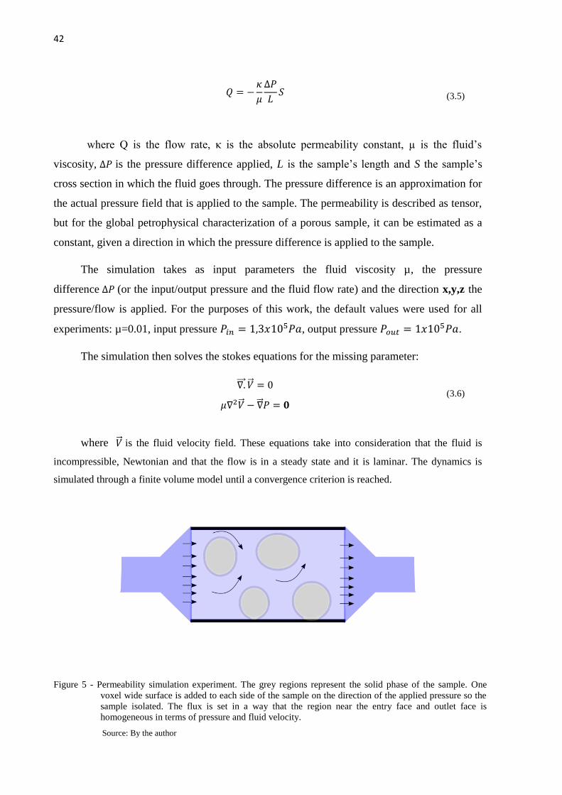
FILTER TO ELIMINATE HIGH FREQUENCY NOISE. ........................................................................................ 40 FIGURE 5 - PERMEABILITY SIMULATION EXPERIMENT. THE GREY REGIONS REPRESENT THE SOLID PHASE OF THE SAMPLE.
ONE VOXEL WIDE SURFACE IS ADDED TO EACH SIDE OF THE SAMPLE ON THE DIRECTION OF THE APPLIED
PRESSURE SO THE SAMPLE ISOLATED. THE FLUX IS SET IN A WAY THAT THE REGION NEAR THE ENTRY FACE
AND OUTLET FACE IS HOMOGENEOUS IN TERMS OF PRESSURE AND FLUID VELOCITY. ........................................ 42 FIGURE 6 - PORE SPACE, PORE AND THROAT DEFINITIONS. (A) THE POROUS SPACE IS DEFINED AS THE EMPTY SPACE IN
THE MATRIX, THE GRAINS COMPOSE THE SOLID SPACE AND SURFACE. (B) EXAMPLE OF DISCRETIZATION OF
THE PORE SPACE, AND DEFINITION OF THE PORE CENTER (RED) AND THROATS (GREEN DASHED LINES)
THROUGHT THE DISTANCE TRANSFORM ON THE PIXELS. .............................................................................. 51 FIGURE 7 - REPRESENTATION OF “SHEET-LIKE” PORE. THE LOCAL MAXIMA WILL BE THE DISTANCE REPRESENTED BY THE
CIRCLE’S RADIUS. THIS SIMPLE REPRESENTATION WON’T BE ABLE TO CAPTURE THE REAL CROSS SECTION OF
THE PORE SPACE WHICH CAN LEAD TO ERROUNEOUS INTERPRETATION OF THE DATA. ....................................... 53 FIGURE 8 - EXAMPLE OF THE PROCESS OF REPEATED EROSION ON A 2D IMAGE. PIXELS THAT ARE ON THE BORDER OF
THE OBJECT ARE CHOSEN FOR REMOVAL. THIS IS DONE INTERACTIVELY UNTIL ONLY ONE PIXEL IS LEFT. ................. 54 FIGURE 9 - EXAMPLE OF MEDIAL-AXIS APPLICATION TO A COMPLEX POROUS STRUCTURE (A) PORE SPACE, (B)
MORPHOLOGICAL SKELETON. THE BRANCHING HAPPENS BECAUSE OF THE SHAPE VARIATIONS OF THE
BORDER PIXELS. ................................................................................................................................. 55 FIGURE 10 - EXAMPLE OF THE STEPS OF THE WATERSHED ALGORITHM. (1) THE VALLEYS REPRESENTS THE LOCAL
MAXIMUM OF THE DISTANCE TRANSFORM. THE FLOODING PROCEDURE WOULD BE A PIXEL NEIGHBOR
CLUSTERING STEP. (2) A TAG IS ASSIGNED TO EACH LOCAL MAXIMUM, SIGNALING DIFFERENT OBJECTS (OR IN
THE PORE SPACE, PORE LOCATIONS). (3) THE CLUSTERING PROCESS ON A REGION CONTINUES UNTIL IT
MEETS A DIFFERENT REGION .THE LIMIT BETWEEN TWO REGIONS ARE CALLED WATERSHEDS. ............................. 55 FIGURE 11 - EXAMPLE OF THE DISTANCE TRANSFORM APPLIED TO THE PORE SPACE MODEL. (A) PORE SPACE (B)
DISTANCE MAP: BLUE ARE THE PIXELS CLOSEST TO THE BORDER (C) THE INVERTED DISTANCE MAP USED AS
ENTRY DATA FOR THE WATERSHED ALGORITHM. ....................................................................................... 56 FIGURE 12 - MAXIMUM SPHERES (MS) ALGORITHM FOR PORE SPACE SEPARATION. (1) PORE SPACE DEFINITION (2)
MAXIMUM SPHERES ARE LOCALIZED (3) MAXIMUM SPHERES ARE TAGGED AS DIFFERENT PORES (4) SMALLER
SPHERES THAT ARE CONNECTED TO A PORE SPHERE IS GIVEN THE SAME TAG AND COMPOSES THE PORE’S
VOLUME. SPHERES THAT SHARE TWO OR MORE PORE TAGS ARE DEFINED AS THROATS. ..................................... 57 FIGURE 13 - EXAMPLE OF EDT APPLIED TO A 2D SLICE OF THE µCT DATA OF A BEREA SANDSTONE SAMPLE. (A) THE
BINARY ORIGINAL IMAGE (B) THE RESULTING EDT. THE COLOR SCALE REPRESENTS THE CALCULATED
DISTANCE OF EACH PIXEL TO THE WALL. .................................................................................................. 60 FIGURE 14 - FINAL NETWORK OF SPHERES. (A) THE ORIGINAL DISTANCE TRANSFORM OF THE IMAGE. (B) THE MAXIMUM
SPHERES FOUND ON THE IMAGE. ........................................................................................................... 61 FIGURE 15 - THE CONSTRUCTION OF THE NETWORK OF REGIONS. TWO SEPARATE NETWORKS ARE CONSTRUCTED: A
NETWORK COMPOSED OF THE COMPLETE SET OF SPHERES (MIDDLE IMAGE) AND A SECOND ONE COMPOSED
ONLY OF THE MEDIAL AXIS SPHERES (RIGHT IMAGE). .................................................................................. 61

FIGURE 16 - THE MODEL USED FOR THE CAPACITY ASSIGNED TO EACH EDGE OF THE GRAPH. THE EDGE’S CAPACITY OF
NODE I TO I+1 WILL BE THE AREA OF THE FULL BLUE CIRCLE ON THE IMAGE, GIVEN BY EQUATION (4.10). ............ 62 FIGURE 17 - EXAMPLE OF THE TWO NETWORKS CONSTRUCTED ON THE 2D SLICE OF THE µCT DATA OF A BEREA
SANDSTONE SAMPLE. ON THE RIGHT IS THE COMPLETE NETWORK, AND ON THE LEFT THE MEDIAL AXIS
NETWORK. THE SPHERES OF THE MEDIAL AXIS NETWORK ARE THE SPHERES CONSIDERED AS PORES IN THE
ALGORITHM, AND THE CYLINDER EDGES ARE THE PATH FOUND BETWEEN THE PORES. ...................................... 63 FIGURE 18 - COMPARISON OF THE NETWORK SHORTEST PATH AND THE SKELETONIZATION PROCEDURE FOR FINDING THE
MEDIAL AXIS. 1-5 ARE EXAMPLES OF THE OVER-BRANCHING PROBLEM MENTIONED BEFORE OF THE EROSION
PROCEDURE. 6- LIMITATION OF FINDING ONE SINGLE PATHWAY BETWEEN PORE NODES. ................................ 64 FIGURE 19 - COMPARISON OF THE NETWORK EXTRACTION METHOD (A) AND A PORE-THROAT NETWORK. ........................... 65 FIGURE 20 - SIMULATED PORE SPACE CONSIDERED FOR FIRST PORE MORPHOLOGY TESTS. THE MEDIUM IS AN IDEAL
SPHERE PACKING OF SPHERES OF EQUAL RADIUS. TO SIMULATE A FULLY CONNECTED PORE SPACE THE
SPHERES ARE SEPARATED BY TWO VOXELS FROM EACH OTHER. (A) SPHERE PACKING WIH SPHERE RADIUS OF
30 VOXELS (B) CROSS SECTION OF THE PACKING. (C) PORE SPACE FORMED. (D) COMPLETE SPHERE’S
NETWORK ACQUIRED FROM THE SPACE. ................................................................................................. 66 FIGURE 21 - COMPARISON OF THE CENTRALITIES SCORES FOR EACH NODE TYPE: PORE NODES, THROAT NODES AND
OTHER NODES IN THE NETWORK. (A) A VISUALIZATION OF THE COMPLETE NETWORK EACH NODE COLOR
REPRESENTS ITS CENTRALITY VALUE. (B) NORMALIZED DISTRIBUTIONS OF CENTRALITIES OF EACH NODE
GROUP (BLACK OTHER NODES, BLUE THROAT NODES AND RED PORE NODES) ................................................. 66 FIGURE 22 - COMPARISON OF THE CENTRALITIES SCORES FOR EACH NODE TYPE (A) BEFORE THE CORRECTION PROCEDURE
(B) AFTER THE CORRECTION PROCEDURE. ............................................................................................... 67 FIGURE 23 - THE EXPECTED EQUIVALENT VOLUME V OF THE PORES IS THE VOLUME OF THE DARKER REGION OF THE
FIGURE. ........................................................................................................................................... 68 FIGURE 24 - RESULTS FOR THE SPHERE PACKING OF FIGURE 20. (A) THE PORE SPACE SEPARATION ACQUIRED THROUGH
THE DEVELOPED METHOD. (B)THE EQUIVALENT RADIUS DISTRIBUTION OF THE PORES. ..................................... 69 FIGURE 25 - SIMULATED IDEAL SPHERE PACKING EXAMPLES. LEFT, SPHERES WITH R=50, MIDDLE R=25 AND RIGHT A
MIXTURE OF SMALL AND LARGE SPHERES: R=10 AND R=25. ..................................................................... 70 FIGURE 26 - PORE-THROAT NETWORK EXTRACTED FROM THE SPHERE PACKING EXAMPLE WITH R=25. SPHERES
REPRESENT THE PORE LOCATIONS, AND THE CHANNELS REPRESENT THE THROATS. THE THROAT’S DIAMETER
FOR ALL CONNECTIONS IS 25 VOXELS. .................................................................................................... 71 FIGURE 27 - SAMPLES USED FOR THE PORE NETWORK EXTRACTION METHOD AND ANALYSIS. (A)-(C) RECONSTRUCTED
VOLUME AND DIMENSIONS OF THE BEREA SANDSTONE, ESTAILLADES CARBONATE AND SYNTHERIZED
SPHERE PACKING SAMPLES. (E)-(F) VISUALIZATION OF THE PORE SPACE FOR THE BEREA, ESTAILLADES AND
SPHERE PACKING SAMPLES. ALL IMAGES WERE OBTAINED BY THE DEVELOPED SOFTWARE, USING PYTHON
MAYAVI.MLAB LIBRARY. ...................................................................................................................... 73 FIGURE 28 - COMPLETE SPHERE CELLS NETWORKS FOR THE THREE POROUS SAMPLES: BEREA SANDSTONE, ESTAILLADES
CARBONATE AND THE SYNTHERIZED GLASS SPHERE PACKING. THE RESULTS SHOW THAT THE DIVISION OF THE
PORE SPACE INTO SPHERE CELLS IS COHERENT WITH THE PORE-SPACE OF EACH SAMPLE. .................................. 74 FIGURE 29 - MEDIAL AXIS NETWORKS FOR THE THREE POROUS SAMPLES: BEREA SANDSTONE, ESTAILLADES CARBONATE
AND THE SYNTHERIZED GLASS SPHERE PACKING........................................................................................ 75 FIGURE 30 - CENTRALITIES OF EACH NODE GROUP: THROAT, PORE AND OTHER BEFORE AND AFTER THE CORRECTION WAS
APPLIED TO THE NETWORK DATA OF EACH SAMPLE. (A) BEREA SAMPLE, (B) ESTAILLADES SAMPLE (C)
SINTHERIZED SPHERE PACKING. EACH NODE GROUP IS NORMALIZED BY THEIR TOTAL NUMBER OF NODES. ........... 76 FIGURE 31 - COMPARISON OF THE PORE DIAMETER MEASURED BY THE DEVELOPED SOFTWARE (NEW METHOD) TO THE
ANALYSIS OF A COMMERCIAL SOFTWARE (PERGEOS). (A) APPLICATION OF THE METHOD TO A BEREA
SANDSTONE SAMPLE. (B) APPLICATION OF THE METHOD TO A ESTAILLADES CARBONATE SAMPLE. ..................... 78 FIGURE 32 - COMPARISON OF THE PORE DIAMETER MEASURED BY THE DEVELOPED SOFTWARE TO THE ANALYSIS OF A
COMMERCIAL SOFTWARE (PERGEOS). (A) APPLICATION OF THE METHODS TO THE BEREA SANDSTONE
SAMPLE. (B) APPLICATION OF THE METHODS TO THE ESTAILLADES CARBONATE SAMPLE (C) APPLICATION OF
THE METHODS TO THE SPHERE PACKING SAMPLE. .................................................................................... 79 FIGURE 33 - COMPARISON BETWEEN GEOMETRICAL AND ELETRICAL TORTUOSITY DISTRIBUTIONS ACQUIRED THROUGH
NETWORK WALK. (A)-(C) SHOW THE GEOMETRICAL TORTUOSITY FOUND FOR THE BEREA SAMPLE,
ESTAILLADES SAMPLE AND SPHERE PACKING SAMPLE RESPECTIVELY. THE GRAPHS (D)-(F) SHOW THE

TORTUOSITY DISTRIBUTION OF THE PATHS CONSIDERING THE DIAMETER OF THE CHANNELS AND THE MEAN
CENTRALITY OF THE NODES. (D) BEREA SAMPLE, (E) ESTAILLADES SAMPLE AND (F) SPHERE PACKING
SAMPLE............................................................................................................................................ 81 FIGURE 34 - ESTIMATED ELECTRICAL TORTUOSITY DISTRIBUTIONS IN COMPARISON TO THE POROSITY PROFILES OF EACH
SAMPLE.(A)-(B) ELECTRICAL TORTUOSITY DISTRIBUTIONS FOR BEREA, ESTAILLADES AND SPHERE PACKING
RESPECTIVELY. THE GRAPHS (D)-(F) SHOW THE POROSITY PROFILES FOR THE BEREA, ESTAILLADES AND
SPHERE PACKING VOLUMES, RESPECTIVELY. ............................................................................................. 82 FIGURE 35 - DISTRIBUTION OF THE EUCLIDIAN DISTANCE BETWEEN PORES AND THE ARC DISTANCE OF THE CONNECTING
CHANNELS. (A) EUCLIDIAN DISTANCE (B) ARC DISTANCE. WE SEE THAT THE DISTANCE BETWEEN PORES IS
SIMILAR FOR THE BEREA AND ESTAILLADES. ON THE OTHER HAND, THE NUMBER OF PATHS WITH A HIGHER
ARC DISTANCE BETWEEN PORES IS MUCH HIGHER FOR THE ESTAILLADES THAN THE BEREA SAMPLE. .................... 83 FIGURE 36 - BEHAVIOR OF THE TORTUOSITY DISTRIBUTIONS FOR EACH SAMPLE IN EACH CHOSEN DIRECTION. ........................ 84 FIGURE 37 - PORE COORDINATION NUMBERS (K) FOR THE BEREA SAMPLE (BLACK) AND THE ESTAILLADES SAMPLE (RED)
SPHERE PACKING SAMPLE (BLUE). (A) DEGREE PROBABILITY DISTRIBUTIONS 𝑃(𝑘) , (B) CUMULATIVE
DEGREE DISTRIBUTIONS 𝑃(𝐾 > 𝑘) COMPARED TO AN EXPONENTIAL DECAY OF THE FORM 𝑃𝑒𝑥𝑝𝑘 = 𝑒 −
𝑘𝑘 , WITH 𝑘 = 5 − 10. ................................................................................................................... 86 FIGURE 38 - FLOW PATHS OBSERVED RESULTING FROM THE PERMEABILITY EXPERIMENT ON Z DIRECTION, SIMULATED ON
THE ORIGINAL VOLUME DATA OF THE SAMPLES ON THE SOFTWARE PERGEOS. LEFT: BEREA SAMPLE,
MIDDLE: ESTAILLADES SAMPLE, RIGHT: SPHERE PACKING SAMPLE. THE COLOR CODING REPRESENTS THE
MAGNITUDE OF THE Z DIRECTION VELOCITY COMPONENT OF THE FLUID, NORMALIZED 0-255. .......................... 88 FIGURE 39 - FLOW PATHS FROM THE SIMULATED PERMEABILITY EXPERIMENT ON THE COMPLETE VOLUME, AND THE
NETWORK MAXIMUM FLOW PATHS FOUND FOR EACH SAMPLE. 1: THE NETWORK COLOR CODED ACCORDING
THE THE EDGE’S TOTAL FLOW CAPACITY. 2- THE NETWORK COLOR CODED ACCORDING TO THE USED
CAPACITY OF EACH EDGE. 3: SIMULATED PERMEABILITY EXPERIMENT (PERGEOS). THE SPHERES REPRESENT
THE INLET AND OUTLET POINTS USED FOR THE MAX FLOW CALCULATIONS ON THE NETWORKS. (A) BEREA
SAMPLE, (B) ESTAILLADES SAMPLE AND (C) SPHERE PACKING SAMPLE. .......................................................... 89 FIGURE 40 - COMPARISON OF THE CURRENT FLOW BETWENNESS CENTRALITY DISTRIBUTIONA OF THE NETWORKS
WITHOUT CONSIDERING THE EDGE WEIGHTS (A) AND CONSIDERING THE EDGE WEIGHTS (B). WE HAVE A
SLIGHT INCREASE OF HIGHER CENTRALITY NODES. ..................................................................................... 90 FIGURE 41 - COMPARISON OF THE CLOSENESS CENTRALITY DISTRIBUTION OF THE NETWORKS WITHOUT CONSIDERING
THE EDGE WEIGHTS ( THE DISTANCE BETWEEN NODES IS THE NUMBER OF STEPS IN THE NETWORK) AND
CONSIDERING THE EDGE WEIGHTS. WE SEE THAT WHEN WE CONSIDER THE EDGE WEIGHTS, THE NUMBER OF
NODES WITH HIGH CLOSENESS CENTRALITY TENDS TO INCREASE. .................................................................. 91 FIGURE 42 - (A) CORRELATION BETWEEN THE MEAN EDGE DISTANCE AND THE NUMBER OF CONNECTIONS OF THE PORES.
(B) CORRELATION BETWEEN THE ARC DISTANCE OF THE EDGES AND THE NUMBER OF CONNECTIONS OF THE
PORE. (C) LOCAL ENTROPY OF EDGE WEIGHTS FOR ALL SAMPLES. ................................................................. 92 FIGURE 43 - CLUSTERING SCORE DISTRIBUTION OF THE NODES FOR EACH SAMPLE. ........................................................... 92 FIGURE 44 - EDGE CAPACITY DISTRIBUTION OF EACH SAMPLE. WE SEE THAT FOR THE ESTAILLADES AND BEREA SAMPLES,
A MAJORITY OF NODES PRESENTED EDGES WITH LOW CAPACITY. THE SPHERE PACKING SAMPLE PRESENTED,
ON THE OTHER HAND, A MORE HOMOGENEOUS DISTRIBUTION. ................................................................... 93 FIGURE 45 - COMPARISON BETWEEN THE MAXIMUM FLOW VARIATION WITH THE TARGET ATTACK FOR THE BEREA AND
SPHERES SAMPLES. ............................................................................................................................. 94 FIGURE 46 - VARIATION OF THE MAXIMUM FLOW (Z DIRECTION) AS PORES WERE REMOVED FROM THE NETWORK. RED
SPHERES REPRESENT THE VARIATION AS THE LARGEST PORES WERE REMOVED, BLACK SQUARES THE
VARIATION AS THE MOST CENTRAL PORES WERE REMOVED. (A) BEREA SAMPLE, (B) ESTAILLADES SAMPLE,
(C) SPHERE PACKING SAMPLE. .............................................................................................................. 94 FIGURE 47 - STRUCTURE OF THE WORMHOLE FORMATIONS FOR EACH SAMPLE. THE GREY SURFACE REPRESENTS THE
WORMHOLES. ................................................................................................................................... 96 FIGURE 48 - MEDIAL AXIS NETWORKS FROM THE WORMHOLE SAMPLES. THE DIAMETER VARIATION OF THE PATHS IS
SHOWN IN COLOR CODE. ..................................................................................................................... 97 FIGURE 49 - DEFINITION OF THE SEPARATION BETWEEN MAIN PATHS AND RAMIFICATIONS, USING SAMPLE E2 AS AN
EXAMPLE. WE DEFINED THE MAIN PATHS AS THE MINIMUM DISTANCE PATHS BETWEEN THE INLET POINTS OF

THE ACID INFLUX TO THE OUTLET POINTS AT THE LIMIT OF THE SAMPLE. ALL OTHER PATHS ARE CONSIDERED
RAMIFICATIONS FROM THE MAIN PATHS. ................................................................................................ 98 FIGURE 50 - RADIUS DISTRIBUTION FROM THE SAMPLES. (A) MAIN PATH RADIUS DISTRIBUTIONS. (B) RAMIFICATION
CHANNELS RADIUS DISTRIBUTIONS (B) COMPARISON BETWEEN RAMIFICATION AND MAIN PATH RADIUS
DISTRIBUTIONS (D) RADIUS VARIATION OF THE MAIN PATHS WITH THE DISTANCE OF THE ACID ENTRY POINT. ........ 99 FIGURE 51 - DEFINITION OF THE SEPARATION BETWEEN MAIN PATHS AND RAMIFICATIONS FOR THE E4 SAMPLE. (A)
COMPLETE SAMPLE COLOR CODED ACCORDING TO THE PATH’S DIAMETER. (B) MAIN PATHS SELECTED FROM
THE SAMPLE, COLOR CODED ACCORDING TO THE PATH’S DIAMETER. (C) MAXIMUM FLOW PASSAGE IN EACH
EDGE. ........................................................................................................................................... 100 FIGURE 52 - TORTUOSITY DISTRIBUTIONS IN THE DIRECTION OF THE ACIDIFICATION FOR EACH SAMPLE. .............................. 101 FIGURE 53 - MEAN FREQUENCY THAT A SITE WAS VISITED IN THE SIMULATIONS FOR EACH SAMPLE. .................................. 102 FIGURE 54 - PERCENTAGE OF THE TOTAL UNIQUE VISITED SITES IN CORRELATION WITH THE SIMULATION TIME FOR EACH
SAMPLE. HERE ONLY THE RESULTS OF THE PARTICLES THAT REACHED THE OUTLET POINTS IN SHOWN. ............... 103 FIGURE 55 - VISUALIZATION OF THE CURRENT FLOW CENTRALITY SCORES FOR EACH SAMPLE. ........................................... 105 FIGURE 56 - VARIATION OF THE MAXIMUM FLOW MEASURED WITH THE REMOVAL OF NODES. (A) NODES WERE
REMOVED ACCORDING TO THE CURRENT FLOW CENTRALITY SCORES. (B) NODES WERE REMOVED ACCORDING
WITH ITS EIGENVECTOR CENTRALITY SCORE. (C) NODES WERE REMOVED RANDOMLY (D) COMPARISON OF
THE ROBUSTNESS TEST FOR SAMPLES E5,E8 AND E9 OF THE RESULTS BY CURRENT FLOW SCORES (BLACK)
AND EIGENVECTOR CENTRALITY SCORES (RED). ...................................................................................... 106 FIGURE 57 - THE MAIN PATH FOR FLUID FLOW, HIGHLIGHTED IN BLACK, FOR SAMPLE E5. WE SEE THAT, TO MAINTAIN
THE CONSERVATION OF MASS, IF THE BLACK PATH IS BROKEN, THE FLOW ISN’S ABLE TO DIVERT TO OTHER
PATHS. .......................................................................................................................................... 107 FIGURE 58 - SEPARATION OF THE PORE SPACE INTO REGIONS OF LARGE RELAXATION TIMES AND SMALL RELAXATION
TIMES. EXAMPLE APPLIED TO THE BEREA SAMPLE. ................................................................................. 111

TABLE LIST
TABLE 1 - SUMMARY OF THE DIFFERENT PORE SPACE SEPARATION APPROACHES. ............................................................. 58 TABLE 2 - PORE-SPACE MORPHOLOGICAL DATA FROM THE SAMPLES. SAMPLES’ POROSITY 𝝓 , THE PORE SPACE
SURFACE AREA S AND VOLUME V, AND THE SPECIFIC SURFACE AREA SSA (SURFACE AREA PER SOLID
VOLUME). ........................................................................................................................................... 74 TABLE 3 - COMPARISON BETWEEN THE TOTAL NUMBER OF PORE-SPACE VOXELS AND THE TOTAL NUMBER OF NODES
OF EACH SAMPLE’S NETWORK. ................................................................................................................. 75 TABLE 4 - COMPARISON BETWEEN THE TOTAL NUMBER OF PORE-SPACE VOXELS AND THE TOTAL NUMBER OF NODES
OF EACH SAMPLE’S NETWORK. ................................................................................................................. 77 TABLE 5 - MEAN PATH TORTUOSITY RESULTS FOR EACH DIRECTION. GEO STANDS FOR THE GEOMETRICAL
TORTUOSITY, EL. STANDS FOR THE ESTIMATED ELECTRICAL TORTUOSITY. .......................................................... 82 TABLE 6 - MEAN PORE SEPARATION FOR EACH SAMPLE: 𝐿 IS THE MEAN OF THE STRAIGHT PATH DISTANCE BETWEEN
EACH PAIR OF PORES IN THE SAMPLE (IDENTIFIED BY THE NEW METHOD). THE QUANTITY 𝝈𝒍𝟐𝐿2 =
𝐿2𝐿2 − 1 IS A MEASURE OF THE STATISTICAL FLUCTUATIONS OF THE DATA. 𝑆 IS THE ARC LENGTH OF THE
DISTANCE BETWEEN PORES, MEASURED USING THE SAME METHOD DESCRIBED FOR THE TORTUOSITY
EVALUATION (THROUGH THE DIJKSTRA ALGORITHM), AND 𝜎𝑠2𝑆2 = 𝑆2𝑆2 − 1 IS THE STATISTICAL
FLUCTUATIONS OF S. ............................................................................................................................. 83 TABLE 7 - TORTUOSITY OF PATHS FOUND MORE FREQUENTLY FOR EACH DIRECTION COMPARED TO THE FORMATION
FACTOR RESULTS. ................................................................................................................................. 85 TABLE 8 - RESULTS FOR THE CALCULATED FORMATION FACTOR (NN) OF THE SAMPLES COMPARED TO THE
APPARENT FORMATION FACTOR ACQUIRED WITH THE SOFTWARE PERGEOS. .................................................... 85 TABLE 9 - MEAN ABSOLUTE PERMEABILITY 𝑝 , SIMULATED ON THE BINARY DATA USING THE COMMERCIAL
SOFTWARE PERGEOS, IN COMPARISON WITH THE MEAN CONNECTIVITY 𝑘 CALCULATED IN THE NETWORK
MODEL. .............................................................................................................................................. 87 TABLE 10 - MAXIMUM FLOW FOUND ON THE NETWORKS COMPARED WITH THE SIMULATED PERMEABILITY 𝑝𝑧 IN Z
DIRECTION. .......................................................................................................................................... 88 TABLE 11 - NUMBER OF NODES REMOVED TO INTERRUPT FLOW THROUGH CLOSENESS CENTRALITY TARGETED ATTACK ............. 93 TABLE 12 - CHARACTERISTICS OF µCT DATA OF THE WORMHOLE SAMPLES. RESOLUTION, NUMBER OF IMAGES SLICES,
VOLUME OF THE SELECTED WORMHOLE, SURFACE AREA OF THE SELECTED WORMHOLE AND THE POROSITY
𝝓 OF THE SAMPLE CONSIDERING ONLY THE WORMHOLE. .............................................................................. 95 TABLE 13 - POROSITY 𝝓 AND ABSOLUTE PERMEABILITY OF THE SAMPLES PREVIOUS TO THE ACIDIFICATION
PROCEDURE ......................................................................................................................................... 95 TABLE 14 - COMPARED RESULTS OF THE MEAN NUMBER OF STEPS NEED TO REACH THE OUTLET POINTS AND THE
NUMBER OF NODES IN EACH NETWORK. .................................................................................................. 104

CONTENT
1 Introduction .................................................................................................................................. 21
1.1 Objectives ..................................................................................................................................... 23
1.2 Thesis organization ....................................................................................................................... 23
2 Complex Networks ........................................................................................................................ 25
2.1 Graph theory ................................................................................................................................. 25
2.2 Centrality Measures ...................................................................................................................... 29
2.2.1 Geodesic paths and the betweenness/closeness centrality ..................................................... 30
2.2.2 Current flow betweenness centrality ........................................................................................ 32
2.2.3 Eigenvector centrality ................................................................................................................ 33
2.2.4 Other local measures ................................................................................................................. 35
3 Samples and Methods ................................................................................................................... 37
3.1 X-ray Computed µTomography .................................................................................................... 37
3.2 Simulations on the volumetric data ............................................................................................. 41
3.2.1 Absolute Permeability ............................................................................................................... 41
3.2.2 Formation factor ........................................................................................................................ 43
3.3 Samples ......................................................................................................................................... 46
3.3.1 Rock samples ............................................................................................................................. 46
3.3.2 Acidification samples - wormholes ............................................................................................ 47
4 Method developed ........................................................................................................................ 49
4.1 Pre-processing .............................................................................................................................. 50
4.2 Definition of pores and throats .................................................................................................... 51
4.3 Construction of the regions network............................................................................................ 59
4.4 Acquisition of the pore morphology ............................................................................................. 65
5 Results ........................................................................................................................................... 73
5.1 Application on rock samples ......................................................................................................... 73
5.1.1 Comparison to commercial methods of pore space analysis .................................................... 78
5.1.2 Global morphology evaluation of the networks ........................................................................ 79
5.1.3 Structural Analysis ..................................................................................................................... 80
5.1.4 Topology study of the extracted networks ................................................................................ 86
5.2 Application on acidification samples - wormholes ...................................................................... 95
5.2.1 Structural analysis ...................................................................................................................... 97
5.2.2 Morphology evaluation through random walk simulation ..................................................... 102
5.2.3 Network robustness evaluation .............................................................................................. 104

6 Conclusions and future work ....................................................................................................... 109
6.1 Future work ................................................................................................................................. 110
References ........................................................................................................................................ 113
21
1 INTRODUCTION
The structure of porous materials is of interest in several areas, from the extraction of oil
and gas1 to agriculture, construction and health. For instance, porous ceramics are used for
water filtration,2 a concern for health issues. Bone is a porous structure, and osteoporosis is
also a major health concern.3 Porous materials are also used to dispose of radioactive waste.
4
Soil is a porous medium, its structure govern water transport, important in agriculture;5
finally, the porous properties of cement is an important area of research on construction.6
The range of approaches to understand the porous structure is proportional to the range of
applications. Two main characteristics are of interest of most areas: porosity and permeability.
Porosity is the bulk volume of the porous space and governs the medium’s storage capacity.
Permeability is a quantification of the ability of a fluid to go through the porous medium.
There are many experimental techniques for the quantification of these properties. Our
group focuses in two: nuclear magnetic resonance (NMR) and digital rock. We have applied
NMR relaxometry on the characterization of siliciclastic rocks,7 cement
8 and collaboration
with work of osteoporosis evaluation.9 A technique for the synthesis of ceramics with
controlled porosity was also developed10
and there is continuous research on the development
of the NMR techniques to observe molecular dynamics inside porous media.11
The Digital Rock front acts as a powerful complementary technique to understand the
characteristics of porous materials. The acquisition of the pore space with high resolution
made possible the development of a realistic simulation of the interactions of the fluid
molecules with the pore space. Through techniques of statistical physics, an algorithm for the
simulation of NMR relaxometry has been developed in our laboratory as well, with great
results.12
One of the questions that remained unanswered, however, is how the interconnection of
the pore space influences the experimental results seen in NMR and other techniques. In order
to answer this question, we propose a statistical analysis of the pore space through the data
acquired through µCT imaging, with the application of complex networks theory.
There have been successful applications of network theory to understand the complexity
of the interconnecting porous space of soils.13
The work of Valentini et al. observed the small

22
world property of fracture networks.14
Other works have compared the fluid flow properties
with the statistical characteristics of fracture networks.15–19
Network models were also used to
understand the dynamics of bacterial leaching through soil.20
Other works focused on the
granular structure of porous media.21-22
Networks have also been applied in the study of bone
structure.23–26
More recently, the work of van der Linden and A. Narsilio were able to
correlate the measurement of the closeness centrality of pores in pore-throat networks to the
permeability of the samples.27
Even though the reduction of the volumetric data from µCT imaging to a network can be
a powerful technique to acquire the main features of the porous structure, there is the question
of what algorithm of network extraction should be used. There are many techniques that have
been developed over the years.23,28–39
Each technique aims at acquiring different features of
the pore space, relevant for the application proposed.
Since our proposal is to understand topological features of the pore space for any porous
media, we needed a general method that was robust and allowed the acquisition of the pore
space morphology with minimum loss of all of its features. For that reason, we developed a
“intermediate” network extraction method in which the pore-space is separated into sphere
cells. This method is based on the well-established maximum spheres algorithm,28,30-31
and
works as an intermediate reduction of the pore-space between the commonly used pore-throat
network and the volumetric data. Through this method we were able to apply network theory
on the networks extracted from samples with very different topologies: sandstone, carbonate
and wormhole formations.
Wormhole is the denomination of a pathway formed after the application of an acid
treatment as a stimulation procedure for the reservoir, a method of EOR (Enhanced oil
recovery). This treatment consists of a reactive fluid flow injected in the inner rock of the
reservoir, which creates a preferential path (wormhole) that optimizes the extraction of the
hydrocarbon fluids.40,41
Therefore, the characterization of the wormhole’s structure is of vital
importance to assess the efficiency of the stimulation procedure.
Knowing that the permeability of rock cores is governed by the number of
interconnections between the pores through pore throats, the developed method is able to
distinguish the regions considered as throats from the regions considered as pores. Instead of
simply based on geometrical properties of the pore-space, the method uses the centrality of
nodes to make this separation.
23
1.1 OBJECTIVES
The main objective of this work is the development of a network extraction method that
could retain and model properties such as tortuosity of the samples and flux through porous
media. Another requirement is that the network extraction should be able to work
independently of the lithology of the samples. To verify this, the method is applied to a
sandstone sample, a carbonate sample, and a glass sphere packing sample. Then the final
networks properties are compared to results from direct simulations on the volumetric data.
Finally, we use network theory to understand how the topology of the samples influences on
the expected permeability and flow.
1.2 THESIS ORGANIZATION
The thesis is organized as follows: On chapter 2 we make a summary of complex
networks theory applied in this work. Chapter 3 presents the samples used and the basis of the
µCT imaging and the simulations on the volumetric data. In Chapter 4 we discuss the
different methods for network extraction and the basis of the developed software. Finally,
chapters 5 and 6 present the results and conclusions of this work respectively.

25
2 COMPLEX NETWORKS
The mapping of complex systems into networks is proving to be a good alternative for
the characterization of their complexity, and the reason behind it is that recent studies of real
life networks are presenting evidences that there is a set of laws which are common to all of
them.
With the development of technology, scientists were able to acquire information from
larger samples of real networks, and very interesting characteristics of these networks started
to emerge. The study of the topology of the Web,42-43
showed that it has properties that
separates it from random graphs, such as the scale free degree distribution, and small world
effect . What was more impressive is that those properties appear to be part of other complex
systems.
As we have discussed before, the application of network theory on porous media has
given promising results into characterizing their structure. In this chapter we will make a short
summary of the basis of graph theory and the measurements applied in this work.43-44
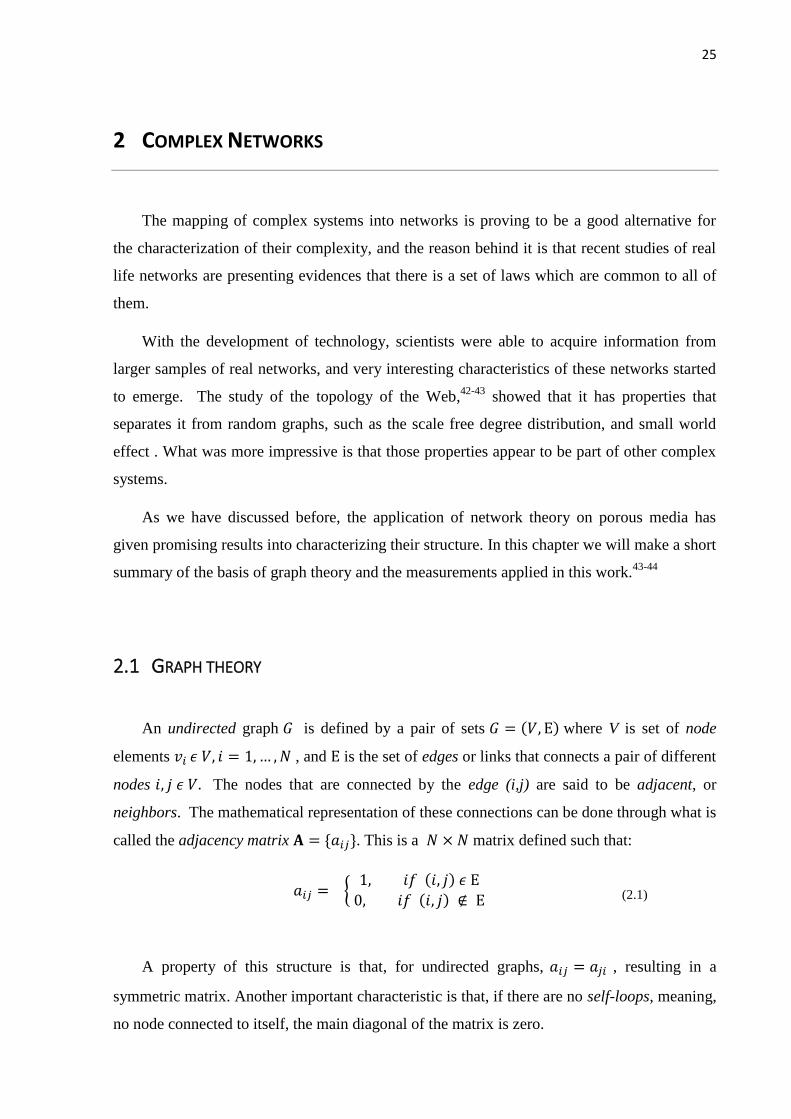
2.1 GRAPH THEORY
An undirected graph 𝐺 is defined by a pair of sets 𝐺 = (𝑉, Ε) where V is set of node
elements 𝑣𝑖 𝜖 𝑉, 𝑖 = 1,… ,𝑁 , and Ε is the set of edges or links that connects a pair of different
nodes 𝑖, 𝑗 𝜖 𝑉. The nodes that are connected by the edge (i,j) are said to be adjacent, or
neighbors. The mathematical representation of these connections can be done through what is
called the adjacency matrix 𝐀 = {𝑎𝑖𝑗}. This is a 𝑁 × 𝑁 matrix defined such that:
𝑎𝑖𝑗 = { 1, 𝑖𝑓 (𝑖, 𝑗) 𝜖 Ε
0, 𝑖𝑓 (𝑖, 𝑗) ∉ Ε (2.1)
A property of this structure is that, for undirected graphs, 𝑎𝑖𝑗 = 𝑎𝑗𝑖 , resulting in a
symmetric matrix. Another important characteristic is that, if there are no self-loops, meaning,
no node connected to itself, the main diagonal of the matrix is zero.

26
Figure 1 - Example of EDT applied to a 2D slice of a Berea sandstone. (a) the binary original image (b) the
resulting EDT. The color scale represents the calculated distance of each pixel to the wall.
Source: By the author
Usually it is useful to assign to the edge a real value, called weight, that represents the
strength of the connection. This value is modelled according to the problem being tackled. For
instance, if the network represents the connection between computers composing the internet,
the edge’s weight can represent the bandwidth of data that can flow between computers. In
this case of weighted networks, the adjacency matrix is not binary, but instead the position
(i,j) represents the weight of the connection of nodes i and j.
Closely related to the adjacency matrix, we have the definition of the graph’s Laplacian.
The definition of the graph Laplacian matrix is given by the diffusion processes in networks.
If we have a substance on the nodes of the network, the node i with the amount Ψ𝑖, the rate at
which the substance Ψ𝑖 changes overtime, given it can move along the edges of the graph, is
described as:
𝑑ψ𝑖
𝑑𝑡= 𝐶 ∑𝑎𝑖𝑗(ψ𝑗 − ψ𝑖)
𝑗
(2.2)
where C is the diffusion constant. So, the equation (2.2) states that the substance will
move along the nodes which are connected, this information given by the adjacency matrix
elements. We can rewrite equation (2.2), splitting into two terms:
𝑑ψ𝑖
𝑑𝑡= 𝐶 ∑𝑎𝑖𝑗ψ𝑗 − 𝐶ψ𝑖 ∑𝑎𝑖𝑗
𝑗𝑗
(2.3)

27
We can make use of the notion of node degree, which is the number of connections the
node has. In an undirected graph, the node’s degree is simply defined as:
𝑘𝑖 = ∑𝑎𝑖𝑗
𝑗
(2.4)
Making use of the result in equation (2.4) on equation (2.3), we can write:
𝑑ψ𝑖
𝑑𝑡= 𝐶 ∑(𝑎𝑖𝑗 − 𝛿𝑖𝑗𝑘𝑖)ψ𝑗
𝑗
(2.5)
𝛿𝑖𝑗 is the Kronecker delta. We can easily see that equation (2.5) can be rewritten in
matrix form:
𝑑𝝍
𝑑𝑡= 𝐶(𝐀 − 𝐃)𝝍 (2.6)
where 𝝍 is the vector whose components are the quantities ψ𝑖 of each node i, A is the
adjacency matrix, and D is the diagonal of the nodes degree:
𝐷 = (𝑘1 0 …0 𝑘2 …⋮ ⋮ ⋱
) (2.7)
Combining the two matrices, we have a new matrix such as:
𝑳 = 𝑫 − 𝑨 (2.8)
And we see that equation (2.6) becomes:
𝑑𝝍
𝑑𝑡+ 𝐶𝑳𝝍 = 0, (2.9)

28
The new matrix L is called the graph’s Laplacian, since (2.9) is the same form as the
diffusion equation for a gas, except that the Laplacian operator ∇2 has been replaced by the
matrix L. Using the definition on equation (2.8), the elements of the matrix L are defined by:
𝐿𝑖.𝑗 = {
𝑘𝑖 , 𝑖𝑓 𝑖 = 𝑗,
−1 , 𝑖𝑓 𝑖 ≠ 𝑗 , (𝑖, 𝑗) ∈ 𝐸, 𝑎𝑛𝑑 𝑖 𝑐𝑜𝑛𝑛𝑒𝑐𝑡𝑒𝑑 𝑡𝑜 𝑗 0 , 𝑜𝑡ℎ𝑒𝑟𝑤𝑖𝑠𝑒,
(2.10)
The graph’s Laplacian is a symmetric real valued matrix. In the context of diffusion,
the spectrum decomposition of L can be used to solve equation (2.9). We can write de vector
𝚿 as a linear combination of the Laplacian eigenvectors 𝐯𝒊:
𝐋𝐯𝒊 = 𝜆𝑖𝐯𝒊, (2.11)
𝝍(𝑡) = ∑𝜙𝑖(𝑡)𝐯𝒊
𝑖
, (2.12)
with the coefficient for the ith
node 𝜙𝑖(𝑡) changing over time and 𝜆𝑖 the eigenvalue
corresponding to the 𝐯𝒊 eigenvector. Substituting into (2.9), we get:
∑(𝑑𝜙𝑖(𝑡)
𝑑𝑡+ 𝐶𝜆𝑖𝜙𝑖(𝑡))
𝑖
𝐯𝒊 = 0, (2.13)
from which we get:
𝑑𝜙𝑖(𝑡)
𝑑𝑡+ 𝐶𝜆𝑖𝜙𝑖(𝑡) = 0, (2.14)
and finally, we can get the variation over time of the coefficients for each node:
𝜙𝑖(𝑡) = 𝜙𝑖(0)𝑒−𝐶𝜆𝑖𝑡,
(2.15)

29
So, given the initial condition of the coefficients and knowing the spectrum of L, we
can solve for the state at any later time. The graph’s Laplacian gives insight on how the
topology of the graph influences in the dynamic of the system.
2.2 CENTRALITY MEASURES
The reach of the diffusion processes in the network will be correlated with the paths
between nodes. A path is defined as a sequence of nodes such that every pair of consective
nodes in that sequence is connected by an edge.
𝑝(𝑢𝑖) = {𝑢𝑖 , 𝑢𝑖+1, 𝑢𝑖+2, … , 𝑢𝑛}, (𝑖, 𝑖 + 1) ∈ 𝐸 (2.16)
Usually, two nodes will be connected by many paths. However, the number of
independent or disjoint paths between two nodes is considerably smaller. Two paths are said
to be independent if they connect the same two nodes but don’t share any edges. The number
of independent paths is a measure of how strongly connected the two nodes are. A highly
connected network is said to be robust, since it is necessary that many nodes or edges are
removed to disrupt the flow of information on this network.
This is easily visualized if we take the internet as an example of a robust network. If just
the connection (edge) to one computer (node) is removed, it is highly unlikely that the flow of
information will stop. However, this will depend on how important this node is. If the node
removed is a computer acting as an internet hub, this will affect the flow of information,
disconnecting other nodes. So, this computer will have a higher centrality on the network.
Moreover, two nodes may not become disconnected even if a large group of edges are
removed. An important measure of connectivity is the minimum cut set, or the minimum
number of edges that, if removed, will disconnect a pair of nodes. If each edge’s weight
represents the maximum flow capacity between this pair of nodes, the maximum flow between
this pair of nodes will be the sum of the weights of the edges of the minimum cut set between
this pair.
The maximum-flow: minimum cut correlation takes in consideration the constraints that
must be followed so the maximum flow can be calculated correctly. If we consider a flow
network G(s,t,c), such that two of its nodes are selected to be the source s and the sink t of
30
flow and each edge (u,v) has a capacity 𝑐(𝑢, 𝑣) > 0 associated to it, we would have the
following constraints:
(a) The flow along an edge cannot exceed its capacity: 𝑓(𝑢, 𝑣) < 𝑐(𝑢, 𝑣);
So, for each edge e there will a be residual capacity associated to it, given a flow f such
as 𝑟(𝑒) = 𝑐(𝑒) − 𝑓(𝑒) . This will originate a new network called the residual network
𝐺𝑟(𝑠, 𝑡, 𝑟(𝑒)) that models the amount of available capacity on the original network G.
(b) The net flow from u to v must be the opposite of the net flow from v to u: 𝑓(𝑢, 𝑣) =
−𝑓(𝑣, 𝑢);
(c) Flow conservation: the sum of incoming flow to a node must be equal to the amount
of flow going out:
∀ 𝑢 ∈ 𝐺, ∑ 𝑓(𝑢, 𝑣)𝑛𝑒𝑢≠𝑣 = 0 , 𝑛𝑒 = 𝑛𝑢𝑚𝑏𝑒𝑟 𝑜𝑓 𝑛𝑒𝑖𝑔ℎ𝑏𝑜𝑟𝑠 𝑜𝑓 𝑣.
(d) The total flow originated in s must be equal to the flow arriving in t.
The residual network 𝐺𝑟(𝑠, 𝑡, 𝑟(𝑒)) is the basis of the Edmonds-Karp algorithm that
finds the maximum flow. The idea of the algorithm is that, while there is a path on the
residual network, such as , 𝑡 ∈ 𝑝(𝑢𝑖)𝑎𝑛𝑑 𝑟(𝑢𝑖, 𝑢𝑖+1) > 0 , the maximum flow isn’t yet
reached. The paths 𝑝(𝑢𝑖) are called augmenting paths.
Applying Edmonds-Karp algorithm to pore-networks can provide the path of
maximum flow of that sample, given a source point and a sink. However, the question
remains of how we can measure the impact of each pore in the path chain. As it was stated
before, the impact of the removal of a hub in a computer network is much larger than
removing and ordinary computer. There are different ways we can score a node’s centrality on
a network, we will discuss in the next session the metrics chosen for this work.
2.2.1 Geodesic paths and the betweenness/closeness centrality
As it was discussed before, the concept of a path is the basis of the definition of distance
between two nodes. Considering an undirected unweighted graph, this distance is simply a
measure of the number of steps one needs to take after departing of the node u to reach node
v. In geographical networks, such as the pore-network, each node has a real position on
tridimensional space. So, instead of simply taking the number of steps between two nodes, we
can measure the real distance that a particle starting from u had to transverse to reach v.

31
However, as we have seen before, there can be many possible paths between nodes u and v.
The shortest path 𝑙𝑖𝑗 between all possible ones is called geodesic path between two nodes.
The typical diameter of a network is defined as the maximum length between all
possible geodesic paths:
𝑑 = max𝑖,𝑗 (𝑙𝑖,𝑗) (2.17)
Through the shortest paths, we can characterize the local influence of the nodes on the
information distribution through the network, namely the nodes’ centrality. One direct
measure of centrality is the node closeness centrality:
𝑔𝑖 =1
∑ 𝑙𝑖,𝑗𝑖≠𝑗 (2.18)
This measure gives larger centrality to nodes that have small shortest path distance to all
others.
Another very relevant measure is how often a node appears in the shortest paths
between other nodes. This measurement is given by the betweenness centrality:
𝑏𝑖 = ∑𝜎𝑘,𝑗(𝑖)
𝜎𝑘,𝑗𝑘≠𝑗≠𝑖
(2.19)
where 𝜎𝑘,𝑗 is the total number of shortest paths that starts from node k and ends in node
j and 𝜎𝑘,𝑗(𝑖) is the number of these shortest paths that go through node i. This measure is
called betweenness centrality because usually nodes with high b will be nodes that act as
bridges between groups of other nodes. Since information, in most cases, passes through
shortest paths, these nodes play an important role on information spread.
Even though the betweenness centrality and closeness centrality already provide
important information on the topology of the networks, we concentrated our efforts into two
more centrality measures. We will explain them further in the next sections.

32
2.2.2 Current flow betweenness centrality
The previous discussed methods of assessing centrality are limited, since they consider
only geodesic paths. This is problematic, since if a path if just slight longer than the geodesic
path it is disregarded and the number of shortest paths that is premediated by each node is not
taken into consideration at all. Another criticism is that information is not able to split
between paths. A solution to account for this information was the development of a centrality
based on current flow.
An electrical network is a graph with positive edge weights indicating either the
conductance or the resistance to the passage of current, note that the conductance and
resistance are related: 𝑐(𝑒) = 1𝑟(𝑒)⁄ for all 𝑒 𝜖 𝐸. Here, we consider a network of resistors,
in which the nodes are the junctions between the resistors.
The Kirchhoff’s law applied to this network, with 𝑉𝑖 the voltage at node i , measured
relative to a convenient reference potential,
∑𝑎𝑖𝑗
𝑉𝑗 − 𝑉𝑖
𝑟(𝑖, 𝑗)+ 𝑏(𝑣) = 0,
𝑗
(2.20)
The current 𝑏(𝑣) represents the external current flowing through node v, due to the
reference nodes s and t that being connected to an external voltage. The node v in which
𝑐 > 0 it is called a source, if 𝑏(𝑣) ≠ 0 it is called an outlet, and the node v in which 𝑏(𝑣) < 0
is called a sink. We will consider the case that a unit current enters the network at a single
source s and leaves it at a single sink t, i.e:
𝑏𝑠𝑡(𝑣) = {1, 𝑣 = 𝑠−1, 𝑣 = 𝑡
0, 𝑜𝑡ℎ𝑒𝑟𝑤𝑖𝑠𝑒 (2.21)
Here, the graph’s Laplacian again dictates the topology’s influence on the total current
flow. Rewriting equation (2.20) we get:
33
∑(𝛿𝑖,𝑗𝑘𝑖 − 𝑎𝑖𝑗)𝑉𝑗 = 𝑅𝑏(𝑣),
𝑗
(2.22)
Or in matrix form:
𝐋𝐕 = 𝒓𝐛 (2.23)
The centrality of each node by using this model of electrical network, needs to be
unique for each node. In other words, the currents that passes in each edge must be unique.
This only happens if we have absolute potentials, such as 𝑝(𝑖, 𝑗) = 𝑝(𝑗) − 𝑝(𝑖) for all node
pairs in G. However, one of the properties of the Laplacian is that at least one of its
eigenvalues is zero, making it a not inversible matrix. This implies that we can add any
multiple of the eigenvector (1,1,1..) to the solution and get another valid solution. In order to
obtain a restricted system, we fix one of the potentials on a selected node as zero (removing
the correspondent column and row from the Laplacian matrix).
Solving (2.23) for the current b of each node, we can define the current flow
betweenness centrality as the sum of the current passing in each edge connecting to its
neighbors. We know that the total throughput in a node i will be:
𝑇𝑖 =1
2(−|𝑏(𝑣)| + ∑|𝑏(𝑖, 𝑗)|
𝑗
) (2.24)
And, accordingly, the measure of centrality, averaged for all node pairs, will be:
𝐶𝐹𝑖 =1
(𝑛 − 1)(𝑛 − 2)∑ 𝑇𝑖
𝑠𝑡
𝑠,𝑡 𝜖 𝑉
(2.25)
2.2.3 Eigenvector centrality
The eigenvector centrality is a variation of the node centrality based on the node’s
degree. The node’s degree is an important measure of centrality since a well-connected node
will most probably belong to most paths of communication of the network. Moreover, when
34
we are analyzing pore networks, the measure of number of connections of a pore is correlated
to how permeable the medium is.
The downside of the degree’s centrality is that it doesn’t differentiate between neighbors.
The node’s centrality score is only based on the number of neighbors, but a more accurate
would be to award a node a centrality proportional to the sum of the centralities of its
neighbors, such as:
𝑥𝑖 = ∑𝑎𝑖𝑗𝑥𝑗 ,
𝑗
(2.26)
If we apply equation (2.26) iteratively throughout the network, assuming as an initial
condition that 𝑥𝑖 = 1 for all i, after n steps, the centralities of each node, in matrix form, are:
𝐱(𝑛) = 𝐀𝒏𝐱(0) (2.27)
Similarly, as done before, the vector 𝐱(0) can be rewritten as a linear combination of the
eigenvector of the adjacency matrix A, 𝐱(0) = ∑ 𝑐𝑖𝐯𝑖,𝑖 and knowing that 𝐀𝐯𝒊 = 𝜆𝑖𝐯𝒊,
𝐱(𝑛) = ∑𝑐𝑖𝜆𝑖𝑛𝐯𝒊
𝒊
(2.28)
There are multiple eigenvectors, in general, that can be applied to (2.28) to get the
centrality score for the node. However, the idea is to ensure that all indices 𝐯𝒊 be positive. As
the adjacency matrix for an undirected graph will always be a real positive square matrix, the
Perron-Frobenius theorem states that the matrix spectrum has a unique positive largest
eigenvalue that the correspondent eigenvector can be chosen to have strictly positive
components. Since 𝜆1 > 𝜆𝑖 , 𝑖 > 1 we get from (2.28):
𝐱(𝑛) = 𝜆1𝑛 ∑𝑐𝑖 (
𝜆𝑖
𝜆1)𝑛
𝐯𝒊
𝒊
(2.29)

35
As 𝑛 → ∞ , we get that the centrality 𝑥(𝑛) → 𝑐1𝜆1𝑛𝐯𝟏 , the limiting vector of the
centralities will be the vector corresponding to the largest eigenvalue of A.
A well-discussed problem of the eigenvector centrality is that it only works well if the
graph is strongly connected. If the nodes have few connections to other, it´s centrality will
rapidly become null in this measure. However, the case of real undirected networks usually,
the largest component is of size proportional to the networks’ size, with nodes well-
connected.
2.2.4 Other local measures
Two other important local measures applied in this work are the clustering score and
the local entropy. The clustering score, although it is a local measurement of a node, it
describes a global feature of the graph, measuring local group cohesiveness. The clustering
score of node i is defined by the ratio between the connectiveness of the nodes adjacent to i to
the total number nodes pairs:
𝑐𝑖 =𝑒𝑖
𝑘𝑖(𝑘𝑖 − 1)/2
(2.30)
where 𝑒𝑖 is the number of connection between nodes adjacent to i and 𝑘𝑖 is i degree,
given that 𝑘𝑖 > 1.
Since we are dealing with weighted graphs in this work, a relevant local measure of the
heterogeneity of the edges’ weights is the local entropy:
𝑓𝑖 = −1
ln (𝑘𝑖)∑
𝑤𝑖,𝑗
𝑠𝑖𝑗∈𝑉𝑖
𝑙𝑛 (𝑤𝑖,𝑗
𝑠𝑖) (2.31)
where Vi is the group of nodes adjacent to i, ki is the node’s degree, wi,j is the edge’s
weight between node i and j and si is the node’s total strength. The strength of a node is
defined as the sum of all edge’s weights connected to it. The local entropy will be 0 if the

36
node’s strength is concentrated in one edge and 1 for a homogeneous distribution between
edges.

37
3 SAMPLES AND METHODS
3.1 X-RAY COMPUTED µTOMOGRAPHY
The X-Ray computed micro-tomography has been used in the characterization of
porous materials since the evolution of the technology permitted the acquisition of
information of the pore space, that is, in the order of micrometers of resolution.45–48
The
process is based on the interaction of the X-Ray beams with the sample’s material. Depending
on the sample’s composition, the degree in which X-Ray beams will penetrate the material
will vary. This will be either by absorption of the photon, by photoelectric effect or by
Compton scattering.
The photoelectric effect is the transmission of energy from a high energetic photon to an
electron in the material, that absorbs this energy and disconnects from the atoms to which it
was bounded. The Compton effect is the interaction of the X-Ray photon to a weakly bounded
electron that changes the original wavelength of light due to loss of energy from the photon
because of the interaction. The variation of the intensity of the x-ray beam due to these
phenomena are described by the Lambert-Beer equation49
:
𝐼 = 𝐼0𝑒−∫𝜇(𝑠)𝑑𝑠
(3.1)
where 𝐼0 is the incident beam, and 𝜇(𝑠) describes the attenuation due to the interaction with
the material along the beam path. The exponential decay correlation with the attenuation
variation is easily understood if we think of the following experiment: let N be the number of
monochromatic (same energy) photons that are able to cross a homogeneous plate with width
∆𝑥. If ∆𝑁 is the number of photons that aren’t able to cross by either effect described before,
the rate of energy loss, due to interaction with the plate will respect the equation:
∆𝑁
𝑁= −𝜇Δ𝑥 (3.2)

38
Equation (3.2) basically tells us that the rate of energy loss will be proportional to the
material length Δ𝑥 and the attenuation constant µ. This case µ is constant because we
considered a homogeneous plate.
Now, if we consider that the width of the plate is infinitesimal, equation (3.2) becomes:
𝑑𝑁
𝑁= −𝜇d𝑥 (3.3)
Considering that we have an intensity I0 correspondent to the number N=N0 of incident
photons incident, we can integrate equation (3.3) which leads to:
ln(𝐼) − ln(𝐼0) = −𝜇x
𝐼 = 𝐼0𝑒−𝜇𝑥
(3.4)
If the material is not homogeneous, the attenuation constant will vary along the sample.
In this case, equation (3.4) becomes (3.1). This difference in attenuation according to the
material type is what allows the identification of different regions on the sample. The
attenuation of the beam will be correlated with the density of the material.
Figure 2 - Schematic of a X-ray tomography. The sample is placed between the X-ray source and the detector
(usually an CCD screen). The beam passes through the sample and the attenuated X-Ray is captured
by the screen. This information is stored and the sample is rotated, so the information can be captured
in all directions.
Source: By the author

39
Usually, the experimental apparatus for lab-based microtomography equipment follows
the schematic of Figure 2. The sample is placed between the X-ray source and the detector
(CCD screen). The generated X-ray beam is in conical form, making geometrical
magnification possible by changing the relative position between the sample and the source,
the limitation being the focal point size and the detector resolution.
The sample is rotated so there can be enough projections to capture the information
from the whole volume. Each projection is stored, and then a reconstruction algorithm uses
this information to create a set of image slices, each slice representing a region (tomo) of the
sample’s volume.
Figure 3 - Example of the output of an image slice after the reconstruction stage. The lighter regions are the
highly attenuated due to the material density. The dark regions are the low density regions, in this
case air inside the pore space.
Source: By the author
The final output after the reconstruction procedure are images such as on the example
shown on Figure 3. This is an image slice of an Indiana limestone rock sample that was
acquired at voxel resolution of 35µm. The grayscale coloring represents the density of
different materials of the sample. The higher the density, lighter will be the color assigned to
the voxel. The bright spots on the image are regions with high density materials. The grains

40
that are represented by voxels in various intensity of grey and the porous region are
represented by the darker regions, the least dense regions of the sample.
After the images are acquired, before the identification of the pore space and image
segmentation, the images undergo a pre-processing filtering stage to remove high frequency
noise that can be residual from the image acquisition procedure. Even though the
reconstruction procedure already provides a smoothing and artifact removal process, there can
be still residual noise in the final images.
In this work, the pre-processing step and the segmentation of the pore space was applied
with the commercial software PERGEOS-FEI (PerGeos) 50
(Figure 4).
Figure 4 - Usage example of the commercial software PERGEOS. Application of Non-Local Means Filter to
eliminate high frequency noise.
Source: Adapted from PErGEOS 50
There are several possible image-processing noise removal filters, such as median and
gaussian filters. The advantage of these filters is that they are fast to apply and the noise
removal is efficient for most cases. However, the application of these filters results in a
completed smoothed image.

41
Since we are mainly interested in the pore region and its morphology, in this work we
applied a Non-Local Means filter. This filtering process has the advantage of removing the
high frequency noise without losing information of the object’s borders. By border we mean
any region with steep transition between two grayscale values. This way we can remove the
noise and preserve as much as possible the morphology of the pore space.
Filtering is an important step because of the segmentation step. Using the same
commercial software, we manually set a threshold value in which any voxel with intensity
under the set value, will be assigned to pore space. This is the binarization step, in which we
transform the grayscale image into binary information where 0 is the grain region, and 1 is the
pore space. If the filtering step is skipped, the binarization step will be prone to errors because
neighboring voxels might have very different intensity values due to high frequency noise.
The filtering step smooths the images so continuous regions will have voxels will similar
grayscale intensities.
3.2 SIMULATIONS ON THE VOLUMETRIC DATA
After the volumetric data is segmented, this information can be used to simulate fluid
flow and current flow inside the pore space in order to estimate petrophysical characteristics
of the samples. In this work, we use the simulations in the volumetric data to observe the
correlation of the topological and morphological features of the networks with the
petrophysics measurements of the samples.
Two simulations were used: the absolute permeability simulation and the formation
factor simulation. All simulations were run on the commercial software PerGeos.
3.2.1 Absolute Permeability
The absolute permeability is a measure of the ability of a porous material to transmit a
single-phase fluid. The relationship between the absolute permeability and the flow rate is
given by Darcy’s law51
:
42
𝑄 = −𝜅
𝜇
∆𝑃
𝐿𝑆 (3.5)
where Q is the flow rate, κ is the absolute permeability constant, µ is the fluid’s
viscosity, ∆𝑃 is the pressure difference applied, L is the sample’s length and S the sample’s
cross section in which the fluid goes through. The pressure difference is an approximation for
the actual pressure field that is applied to the sample. The permeability is described as tensor,
but for the global petrophysical characterization of a porous sample, it can be estimated as a
constant, given a direction in which the pressure difference is applied to the sample.
The simulation takes as input parameters the fluid viscosity µ, the pressure
difference ∆𝑃 (or the input/output pressure and the fluid flow rate) and the direction x,y,z the
pressure/flow is applied. For the purposes of this work, the default values were used for all
experiments: µ=0.01, input pressure 𝑃𝑖𝑛 = 1,3𝑥105𝑃𝑎, output pressure 𝑃𝑜𝑢𝑡 = 1𝑥105𝑃𝑎.
The simulation then solves the stokes equations for the missing parameter:
∇.⃗⃗⃗ �⃗� = 0
𝜇∇2�⃗� − ∇⃗⃗ 𝑃 = 𝟎
(3.6)
where �⃗� is the fluid velocity field. These equations take into consideration that the fluid is
incompressible, Newtonian and that the flow is in a steady state and it is laminar. The dynamics is
simulated through a finite volume model until a convergence criterion is reached.
Figure 5 - Permeability simulation experiment. The grey regions represent the solid phase of the sample. One
voxel wide surface is added to each side of the sample on the direction of the applied pressure so the
sample isolated. The flux is set in a way that the region near the entry face and outlet face is
homogeneous in terms of pressure and fluid velocity.
Source: By the author

43
3.2.2 Formation factor
There are many different measurements that are routinely done in the petroleum
industry to estimate the quantity/type of hydrocarbonate fluids and the production of a
reservoir. 52
Amongst these is the measurement of permeability of the rock, that was discussed
before, and the electrical resistivity log, which is used to calculate the porosity and the
saturation of the reservoir rock. The laboratory characterization of the electrical resistivity is
usually done by the measurement of the bulk resistivity of a rock core saturated with brine
solution. The formation factor of the sample is defined as:
𝐹 =𝑅0
𝑅𝑙 (3.7)
where 𝑅0 is the bulk measurement of resistivity and 𝑅𝑙 is the known liquid resistivity.
There are many physical properties that will be correlated to the resistivity
measurements, such as the conductance of the solid surface and the fluid characteristics that
permeates the porous space. However, there is also a dependence on the rock’s lithology such
as the porosity. This dependence was first defined by Archie, 194253
:
𝐹 = 𝐶𝜙−𝑚 (3.8)
where 𝜙 is the porosity of the sample and m is called the cementation factor.
Equation (3.8) is often referred to as Achie’s Law. The determination of the cementation
factor has been theme of discussion in the scientific community52,54–58
. It depends on the
rock’s lithology (sandstones will have different cementation factors than bioclastic
carbonates, for instance). Also, more recent studies agree that the C factor on (3.8) is
correlated with the sample’s tortuosity 56,59–62
:
𝐹 = 𝜏𝛼𝜙−𝑚 (3.9)
44
where τ is the tortuosity, F is the formation factor and ϕ is the porosity of the sample.
The factor α may change according to the rock’s heterogeneity. 54,63
However, the definition of tortuosity is also an open question. Usually, there are four
possible definitions of tortuosity that depends on the application 59-60,62
: geometric, electrical,
hydraulic and diffusive.
Geometric tortuosity is usually defined as the ratio of the mean length of all flow paths
through the medium and the straight-line length across the medium:
𝜏𝑔 =⟨𝐿𝑓𝑙𝑜𝑤⟩
𝐿𝑙𝑖𝑛𝑒
(3.10)
This definition does not take into account that the particles may follow preferential
paths of flow, given the different cross-section diameters of the paths. To account for that, the
hydraulic tortuosity was defined. The hydraulic tortuosity is given by the ratio of a flux-
weighted average path length ⟨𝐿ℎ⟩ = 𝑁𝐿ℎ to the straight-line length, where N is the number
of streamlines going through that path:
𝜏ℎ =⟨𝐿ℎ⟩
𝐿𝑙𝑖𝑛𝑒
(3.11)
Closely related to the hydraulic tortuosity, we have the electrical tortuosity:
𝜏𝑒 =⟨𝐿𝑒⟩
𝐿𝑙𝑖𝑛𝑒
(3.12)
where ⟨𝐿𝑒⟩ is the average electrical flux path length. The tortuosity correlated to the
previous discussed formation factor would be the electrical tortuosity. The electrical tortuosity
and hydraulic tortuosity are usually larger than the geometric tortuosity. The reason is that the
conductance of the paths will take an important role in their determination. So, even if a path
is longer than another in geometrical terms but its conductance is higher than the rest, the
tendency is that the flow will choose to pass through it.
45
The diffusive tortuosity is usually defined as the ratio of the diffusing species in free fluid
df to the restricted diffusion on the tortuous paths inside the porous medium dp:
𝜏𝑑 =𝑑𝑓
𝑑𝑝
(3.13)
The restrictive diffusion coefficient can be determined by NMR relaxometry 64
.
In this work, we focused on the electrical tortuosity, so we could correlate to the
formation factor simulations. The simulation is done by applying a constant electric potential
difference on two opposing faces of the sample. The other faces are considered closed by an
electric insulator. So, the simulation solves for the current flux:
𝑗𝑡𝑜𝑡
𝑆= 𝜎
𝑉𝑖𝑛 − 𝑉𝑜𝑢𝑡
𝐿
(3.14)
where jtot is the current flux going into the sample, S is the sample’s cross section area,
σ is the electrical conductivity of the material, Vin is the input imposed electrical potential,
and Vout the output electrical potential. Two border conditions are imposed: that the sample is
homogenous (σ doesn’t vary in space) and the sample is completely saturated.
To find the conductivity of the saturating fluid, Ohm’s law is applied:
𝑗𝑡𝑜𝑡 = ∫ −𝜎𝑠𝑜𝑙𝑢𝑡𝑖𝑜𝑛∇⃗⃗
𝑆
𝑣 𝑑𝑆 (3.15)
Where v is the electric potential.

46
3.3 SAMPLES
3.3.1 Rock samples
We applied the extraction method to samples with very different lithology with two
objectives in mind. The primary objective was to validate the developed software of network
extraction. Secondly, by choosing samples with very different petrophysical characteristics,
we wanted to evaluate the correlation of the networks structural and functional properties to
the measured petrophysical characteristics of the samples.
The porous media used in this part of the work were composed by two rock samples: a
sandstone (Berea) and a carbonate sample (Estaillades). Another porous sample used was an
artificially constructed porous medium composed by the packing of glass spheres. This was a
sample prepared for the study of molecular diffusion through NMR measurements and
simulations, work done by our colleague PhD candidate Everton Lucas de Oliveira, and was
also used in this work. The diameter variation of the glass spheres used was 150µm to 300µm.
The Berea sandstone is well established in literature as having a homogenous structure,
and is often used as a reference material 65,66
. It is a sedimentary rock whose grains are
predominantly sand-sized and composed of quartz held together by silica.
The Estaillades limestone, (Estaillades, France), in the other hand, has a more complex
porous matrix. It is a bioclastic limestone, meaning that its structure is formed from fossil
fragments or other organisms as well. It is composed of more than 99% calcite 67–69
The µCT images of the Berea sample and the sphere packing sample were obtained by
our group, with voxel resolution of 3.3 µm and volume dimensions of 505x362x532 for the
Berea sample, and 504x504x750 for the sphere packing sample, with voxel resolution of 3.0
µm. The Estaillades sample was downloaded from the Digital Rock Portal. 70
The sample also
has voxel resolution of 3.3 µm and its volume dimensions are 650x650x650.

47
3.3.2 Acidification samples - wormholes
The productivity of a reservoir is of major importance in the oil industry. There are
various factors which can lower a reservoir’s productivity. The rock formation with low
porosity region, due to lamination on its formation, might induce low permeability in the
direction of the fluid extraction and even the drilling itself may cause damages to the reservoir
that reduces its productivity.
One of the stimulation procedures that is often applied to carbonate reservoirs is the acid
treatment, because of the high reaction of the acid to the carbonate formations. It consists of a
reactive fluid flow that is injected to the inner rock of the reservoir. This procedure creates a
conductive preferential path, known as wormhole, that optimizes the extraction of the
hydrocarbon fluids. 71
However, determining the efficiency of the technique is a difficult task. There is the
question of the optimum pathway formation for maximum fluid extraction, with minimum use
of acid. For this determination, there are many variables involved: the total volume of acid
used, the original petrophysical characteristics of the rock and the injection rate. All these will
influence on the formation of the wormhole pathway's morphology. Therefore, the
characterization of the wormhole’s topology is of vital importance to assess the efficiency of
the method
All the acidification samples were acquired through a joint project with
Petrobras/Cenpes. The acidification and imaging was done by the Cenpes team. The samples
are composed by 5 Indiana Limestones rock plugs (E2, E4, E5, E8, E9) (region of Indiana,
US). Each sample is cylindrical, with 3.8 cm of diameter and 7cm in length. All samples were
treated with HCl, with injection rate 10cc/min. The µCT images were acquired at 40µm
resolution (with some variations), so the wormholes could be visualized.

49
4 METHOD DEVELOPED
Even though the volume extracted from the µCT images can be directly used in fluid
flow simulations, there are advantages on the simplification of the volumetric data by
describing it as a network. One is simply the amount of computer resources needed to
simulate directly into the total captured volume of the pore space. The complex system of the
porous structure for a small sample of millimetric size can be composed of millions of voxels
or even larger.
Moreover, the simplification of the volume into a network opens the possibility of
capturing information of the morphological and topological features of the porous structure. If
we can simplify the complex porous space problem into basic elements and the interaction
between these elements, we could find common features between porous samples. This can
help us understand the process that lead to their shape and formation and how their structure
influences on the dynamics of the permeating fluid.
When we are dealing with flow in porous media, two main features are of interest: pore
sizes, which are the regions that the fluid is stored and the connection between pores, which
limits the extraction of the fluid inside the rock. These two characteristics differ from the
sample’s morphology (size and shape of the pores) and the samples topology (position of the
pores and how they are connected).
This is the main motivation for our study of the different algorithms of network
extraction and the development of a new method. In general, the algorithms either focus on
the total topology of the sample through medial axis methods, or focuses only on the
separation of pores and throats, oversimplifying the samples’ topology.
To reduce the information loss, we have proposed a new way of viewing the
interconnection of pores. We use the well stablished maximum spheres algorithm to divide
the pore space into sphere cells. This allows a simplification of the pore space with minimum
original data loss. The sphere cells are connected as a graph, leading to a complex network of
regions. The final algorithm doesn’t ignore that knowing the position of the regions
considered as pores, and their morphology is an important information. We see as well, the
importance of knowing the regions of constriction, which can limit the extraction of fluid

50
from the pores. So, a pore-throat separation method is also proposed, which aims to be
applicable to any porous medium. Here, we will first discuss the main methods used for pore-
network extraction from µCT data: medial axis, watershed algorithm and the maximum
spheres algorithm. Then the proposed method will be presented.
This chapter is organized as follows: First the pre-processing steps required for the
network extraction are presented, then the different approaches for pore space separation will
be presented and finally the proposed alterations to the Max Ball algorithm will be discussed
and the final algorithm of the developed software is shown.
4.1 PRE-PROCESSING
The data from the µCT scanners is usually stored as a set of 2D images. To use this
information to extract the morphological characteristics of the porous matrix, is necessary first
to reconstruct these images into volumetric data. There are several software that perform this
task, such as ImageJ, which is a open source software, free to download.
Each volumetric point is called voxel ( 𝑣𝑖 = 𝑣(𝑥𝑖 , 𝑦𝑖, 𝑧𝑖) ), where 𝑥, 𝑦, 𝑧 𝜖 𝐍𝟑 are
coordinates on the tridimensional space. The voxel is the equivalent to the pixel, in volumetric
objects. It will represent the intensity on each point of the space.
When we are dealing with porous media, each voxel will either represent void space or a
specific kind material. Since we are interested on the void portion, we segment the
volumetric data into void voxels 𝑣𝑣𝑜𝑖𝑑 and material representative voxels 𝑣𝑚𝑎𝑡𝑒𝑟𝑖𝑎𝑙 . Void
voxels are defined as follows:
𝑣𝑣𝑜𝑖𝑑𝑖 = 𝑣𝑖 ∈ 𝑁| 𝑣𝑖(𝑥, 𝑦, 𝑧) < 𝑡, 𝑖 = 0,1,2, …𝑁
𝑁 = 𝑡𝑜𝑡𝑎𝑙 𝑛𝑢𝑚𝑏𝑒𝑟 𝑜𝑓 𝑣𝑜𝑥𝑒𝑙𝑠 (4.1)
Where t is a threshold parameter, a greyscale level set by the user that sets all the voxels
under a defined limited of brightness into pore space. There are several proposed methods to
choose this threshold value.

51
Now the volumetric data is segmented into voxels that belong to the pore space and to the
sample material. This is the input data for all digital rock experiments, so minimum loss of the
original data on the segmentation procedure described above is paramount. As we discussed
before, usually this is achieved by using minimum loss filters on the original µCT images
before the segmentation procedure, such as Non-Local Means.
4.2 DEFINITION OF PORES AND THROATS
After the pore space is defined by the volume segmentation described before, the space
can be further simplified by capturing the two main entities that will be the descriptors of the
fluid flow: pores and throats.
The identification and separation of pores and throats in the final volume is a difficult
problem, but before discussing the different approaches for the pore-network extraction, we
need first a definition of what will be considered a pore and a throat in the volumetric pore
space. The most accepted definition of a pore is a wide region of the pore space that is limited
by narrowing regions, namely throats. So, the pores’ total volume is representative of the bulk
volume of the permeating fluid and the throat radii are representative of the capillary
pressures.
A more precise description of this definition has been done by M. J. Blunt, 2017 51
,
through a mathematical model that defines the position of a pore’s center.
Figure 6 - Pore space, pore and throat definitions. (a) The porous space is defined as the empty space in
the matrix, the grains compose the solid space and surface. (b) Example of discretization of
the pore space, and definition of the pore center (red) and throats (green dashed lines) through
the distance transform on the pixels.
Source: By the author

52
The pore space, as shown on a 2D representation on Figure 6 (a), is a continuum space
with complex morphology. The pore center is represented by the red pixel on Figure 6 (b) and
the throats are the dashed green lines. To find the position of the pore’s center, we apply to
the image an operator called distance transform. The distance transform assigns to each object
pixel the distance between its position and the nearest border pixel, such as:
𝐷𝑇(𝑣𝑣𝑜𝑖𝑑𝑖 ) = min
0<𝑘<𝑁𝑏𝑜𝑟𝑑𝑒𝑟(‖𝑣𝑣𝑜𝑖𝑑
𝑖 − 𝑣𝑏𝑜𝑟𝑑𝑒𝑟𝑘 ‖)
(4.2)
If we considered the pore space as a continuum, the local maxima, minima, or saddle
point of the continuous distance transform would be the points (x,y) in which the gradient of
the transform is zero, such as:
𝛁𝑑(𝑥, 𝑦) = 𝐠 = 0 (4.3)
The local maxima will be defined amongst these extreme points as the positions (x,y) in
which the second derivative is negative. In more general terms, the local maxima would be
the positions in which the eigenvalues of the Hessian matrix are all negative:
H𝑖,𝑗 =𝜕𝑑(𝑥𝑖, 𝑥𝑗)
𝜕𝑥𝑖𝜕𝑥𝑗
H𝑖,𝑗𝑒𝑗 = 𝜆𝑒𝑗
(4.4)
The position of the local maxima can be considered the pore centers, in other words, the
regions where the bulk fluid will be concentrated.
The definition of the throat’s centers, on the other hand, can be a more difficult task. M.
J. Blunt, 2017 51
, imagines a streamline starting from pore i and ending on pore j in which the
direction of this line is always parallel to the gradient field g. The throat would be the surface
perpendicular to the regions of saddle point that belongs to this streamline.
Even though these definitions are straightforward for a continuous medium, the
application to digital rock samples encounters several difficulties. The local maxima in a

53
discreet region may not be well defined (two or more neighboring voxels can have similar
distance to the walls). There is also the question of recovering the pore’s morphology (the
shape and geometry), which holds important information of the sample’s formation.
Moreover, for sheet like pores, the local maxima won´t be representative of the real cross
section of the pore space (Figure 7).
Figure 7 - Representation of “sheet-like” pore. The local maxima will be the distance represented by the
circle’s radius. This simple representation won’t be able to capture the real cross section of
the pore space which can lead to errouneous interpretation of the data.
Source: By the author
The task of capturing the correct shape of the pores and throats, as well as the complete
topology of the sample has been tackled by three main approaches: volumetric medial axis,
distance transform combined to watershed methods and finally the maximum spheres
algorithm. These three approaches usually are interconnected and each has its limitations
which we will discuss here briefly.
The medial axis approach tries to reduce the volume of pores into a topological
equivalent of interconnected lines. This is done by the morphological operation of Erosion on
the tridimensional pore space.72-73
Erosion, as the name states, is an operator that erodes away
the boundaries of the regions considered as objects in a volume.
Let A be a binary matrix representing an image in which the object of interest (the pore
space) is represented by voxels set as one and the solid matrix represented by voxels set as
zero. In this case, the object of interest is the pore space. The erosion takes two pieces of
information as input: the binary matrix A and a structuring element B. This structuring
element is also a binary matrix that defines the neighboring region of the voxel a in the border
of A that should be eroded. If X is the subset of coordinates of the object voxel positions on A,
the mathematical definition of erosion would be:

54
𝐴 ⊝ 𝐵 = {𝑥 ∈ 𝑋|𝐵𝑥 ⊆ 𝐴} (4.5)
Where Bx defines the translation of B to the center point in x. Basically, the erosion
operation on A defines the removal of pixels that are in the border of the object, limited by the
structuring element B. The medial axis is acquired by the repeated erosion, done pixel by
pixel, in the object, until the current pixel has at least two neighboring background pixels.
Figure 8 - Example of the process of repeated Erosion on a 2D image. Pixels that are on the border of the object
are chosen for removal. This is done interactively until only one pixel is left.
Source: By the author
After the procedure is done, the result is called the morphological skeleton of the image.
This process is interesting because it preservers the original topology of the pore, capturing
the tortuosity of the space. However, the definition of pores can be ambiguous. The frequently
used method to define pores on the skeleton are the regions where the skeleton branches into
two or more pathways. The problem with this approach is that these regions of branching
aren’t necessarily regions of larger volume. In fact, the branching regions could be more
representative of throats than pores.
This ambiguity on the pore definition can be visualized on Figure 9. The shape of the
border of the region creates subdivision of the skeleton into multiple branches. Even though
there are many proposed methods to remedy the over branching of the medial axis with good
results on porous media, 25,74–77
there is still the problem of losing the information on the
pore’s original shape. Usually the recovering of the pore’s shape is done by applying the
watershed algorithm to the treated data of the skeleton.
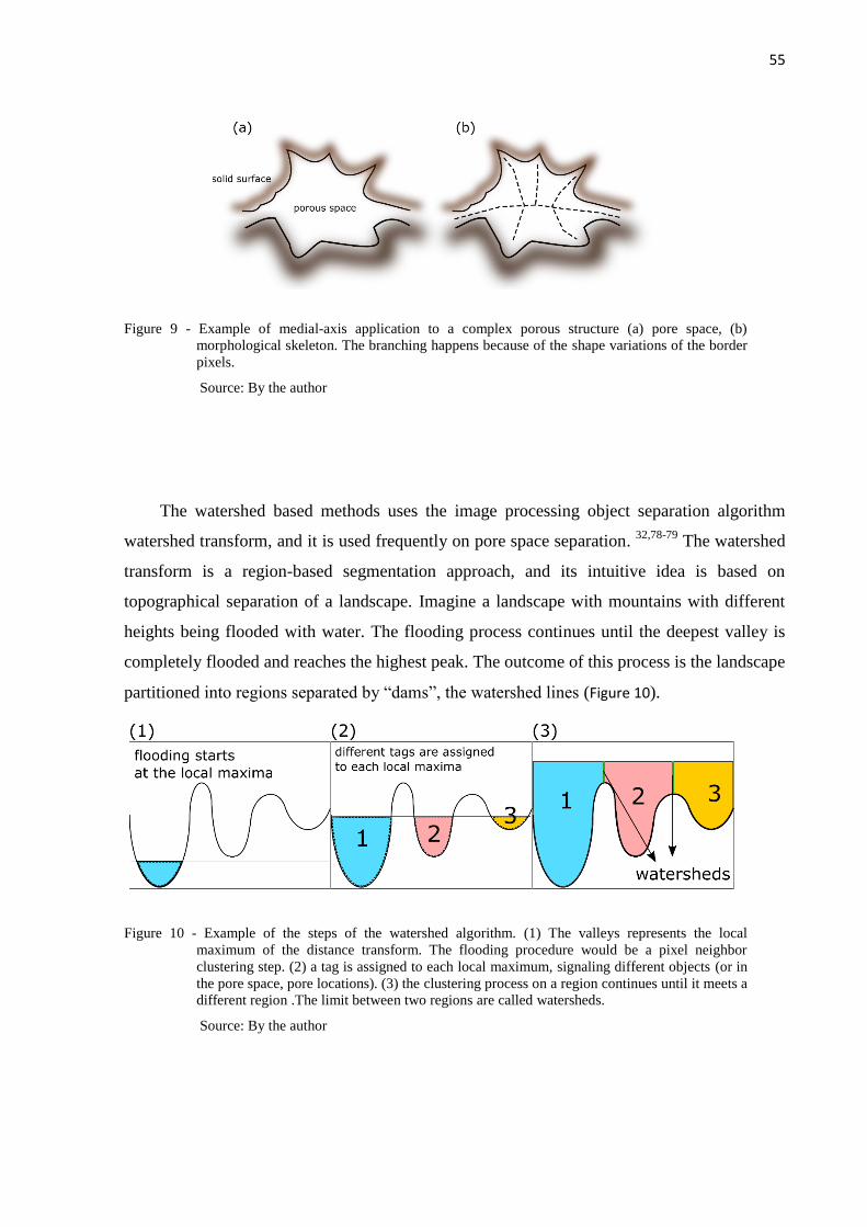
55
Figure 9 - Example of medial-axis application to a complex porous structure (a) pore space, (b)
morphological skeleton. The branching happens because of the shape variations of the border
pixels.
Source: By the author
The watershed based methods uses the image processing object separation algorithm
watershed transform, and it is used frequently on pore space separation. 32,78-79
The watershed
transform is a region-based segmentation approach, and its intuitive idea is based on
topographical separation of a landscape. Imagine a landscape with mountains with different
heights being flooded with water. The flooding process continues until the deepest valley is
completely flooded and reaches the highest peak. The outcome of this process is the landscape
partitioned into regions separated by “dams”, the watershed lines (Figure 10).
Figure 10 - Example of the steps of the watershed algorithm. (1) The valleys represents the local
maximum of the distance transform. The flooding procedure would be a pixel neighbor
clustering step. (2) a tag is assigned to each local maximum, signaling different objects (or in
the pore space, pore locations). (3) the clustering process on a region continues until it meets a
different region .The limit between two regions are called watersheds.
Source: By the author
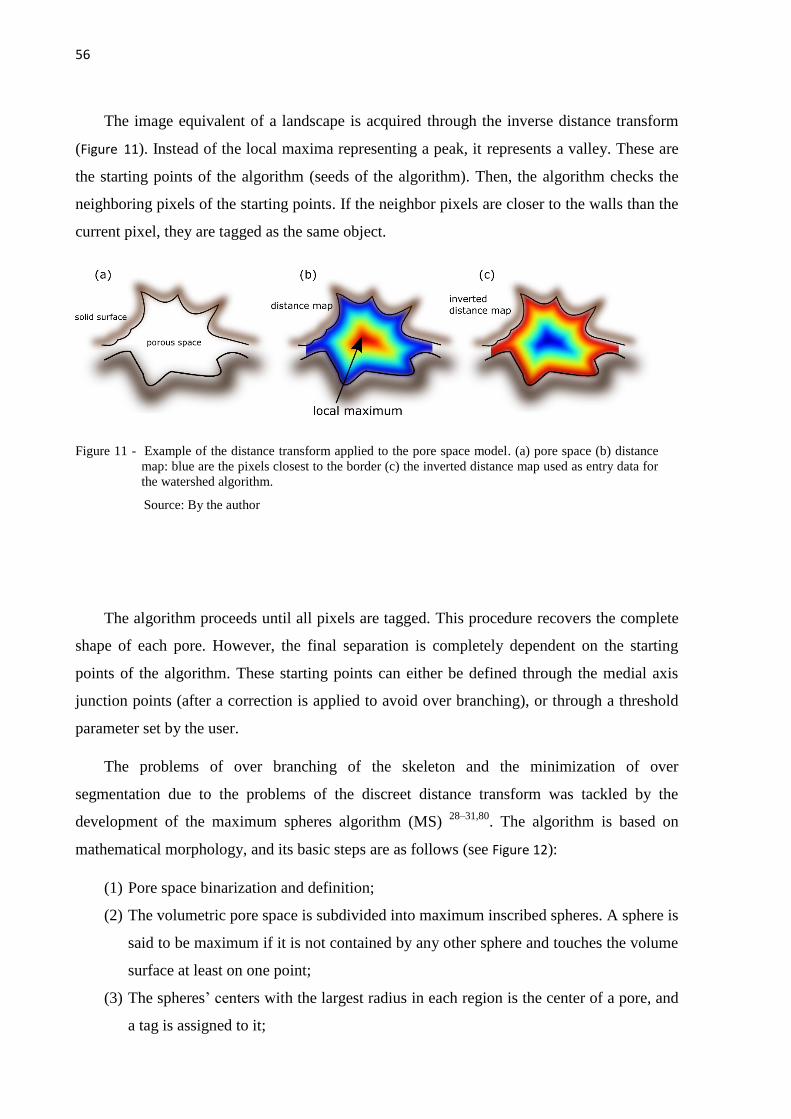
56
The image equivalent of a landscape is acquired through the inverse distance transform
(Figure 11). Instead of the local maxima representing a peak, it represents a valley. These are
the starting points of the algorithm (seeds of the algorithm). Then, the algorithm checks the
neighboring pixels of the starting points. If the neighbor pixels are closer to the walls than the
current pixel, they are tagged as the same object.
Figure 11 - Example of the distance transform applied to the pore space model. (a) pore space (b) distance
map: blue are the pixels closest to the border (c) the inverted distance map used as entry data for
the watershed algorithm.
Source: By the author
The algorithm proceeds until all pixels are tagged. This procedure recovers the complete
shape of each pore. However, the final separation is completely dependent on the starting
points of the algorithm. These starting points can either be defined through the medial axis
junction points (after a correction is applied to avoid over branching), or through a threshold
parameter set by the user.
The problems of over branching of the skeleton and the minimization of over
segmentation due to the problems of the discreet distance transform was tackled by the
development of the maximum spheres algorithm (MS) 28–31,80
. The algorithm is based on
mathematical morphology, and its basic steps are as follows (see Figure 12):
(1) Pore space binarization and definition;
(2) The volumetric pore space is subdivided into maximum inscribed spheres. A sphere is
said to be maximum if it is not contained by any other sphere and touches the volume
surface at least on one point;
(3) The spheres’ centers with the largest radius in each region is the center of a pore, and
a tag is assigned to it;

57
(4) Other spheres that touches a pore sphere, are assigned the same tag and are said to
belong to the same pore. This tag is passed through to neighboring spheres
interactively. This is similar to a breath-first search on a graph. Each sphere with
smaller radius that is connected (by touching another in some point) to another with
larger radius is given the same tag. This procedure is often compared to the pore’s
“family name” being passed through to the smaller spheres that compose its volume.
(5) If a sphere already tagged is found by a sphere with a different ‘family name’, this
sphere is tagged as a throat, or connection between pores.
Figure 12 - Maximum spheres (MS) algorithm for pore space separation. (1) pore space definition (2)
maximum spheres are localized (3) maximum spheres are tagged as different pores (4) smaller
spheres that are connected to a pore sphere is given the same tag and composes the pore’s
volume. Spheres that share two or more pore tags are defined as throats.
Source: By the author
This method is an elegant solution to the main problem with the previous approaches: the
over-segmentation of the pore space due to the shape of its borders. As we have shown
before, the direct application of the erosion procedure and watershed transform on the voxels
can lead to over-branching and to over-separation respectively. The MS algorithm gives an
intermediate step between processing the voxels directly and separating the pore space,
reducing problems with noise in the pore-grain interface.

58
Another important advantage of this process is that there is no loss on the pore’s
morphology. Since we can divide the pore-space into spheres as small as the image resolution,
with proper guidelines, the complete surface of the pore is recovered and assigned to each
individual pore. However, even though there is considerable reduction on errors due to the
pore’s surface shape, there can be still issues with over segmentation due to the definition of
the throat spheres. Since the only condition on a sphere being assigned as a throat is that it
will belong to two (or more) pore families, a small variation on the pore’s surface can lead to
a region being separated into two different ones. Usually this is corrected by setting a
threshold parameter, limiting the size of a sphere that can be considered as throat30
:
𝑟𝑡ℎ𝑟𝑜𝑎𝑡𝑗
𝑟𝑝𝑜𝑟𝑒𝑖
< 𝜆, 0 < 𝜆 < 1
(4.6)
Equation (4.6) states that the ratio between the radius 𝑟𝑡ℎ𝑟𝑜𝑎𝑡𝑗
of a throat sphere j to the
radius 𝑟𝑝𝑜𝑟𝑒𝑖 of all i pores it connects must be lower than a threshold value 𝜆. If it isn’t, the
smallest of the pore sphere’s is merged with the largest neighboring pore. This can be
problematic since different choices of 𝜆 between implementations of the algorithm can
provide different results on the pore-throat separation for the same sample, which in turn, can
lead to different interpretations of the pore structure.
We have summarized the three approaches positive outcomes and issues on Table 1.
Table 1 - Summary of the different pore space separation approaches.
Algorithm Positive outcomes Problems
Medial axis Topological description of the
medium.
Over-branching;
Loss of morphology (can be remedied by the
use of watershed);
Dependent on user tuned parameters
Watershed+distance
transform
Morphological description of
the pores.
Over-segmentation;
Loss of topology;
Dependent on user tuned parameters
Maximum Spheres Morphological description of
the pores;
Avoids over segmentations
Loss of topology;
Dependent on user tuned parameters
Source: By the author

59
Based on the positive outcomes of the MS algorithm, we propose studying the
morphology of our samples based on its concepts. The idea is to use the segmentation of the
pore space into spheres instead of working directly with the voxel data. In the next section of
this chapter the MS algorithm will be presented in more detail and the proposed method for
capturing both the pore-space morphology and topology through network analysis.
4.3 CONSTRUCTION OF THE REGIONS NETWORK
After the pre-processing, the volumetric data becomes binary information, so we can see
the pore space in a True/False perspective. Since our region of interest is the void space, we
set the final tridimensional matrix as:
𝑣𝑣𝑜𝑖𝑑𝑖 = 𝑣𝑖 ∈ 𝑁| 𝑣𝑖(𝑥, 𝑦, 𝑧) = 1
𝑣𝑚𝑎𝑡𝑒𝑟𝑖𝑎𝑙𝑖 = 𝑣𝑖 ∈ 𝑁| 𝑣𝑖(𝑥, 𝑦, 𝑧) = 0
(4.7)
The original MS algorithm does a search on each of the pore space voxels to find the
maximum inscribed sphere with each voxel as center. In the developed software, this step is
done by performing a Euclidean Distance Transform (EDT) on the volumetric data.
As we discussed before, DT is a known transform for binary image processing. It sets to
each pixel on the image, that is considered as an object of interest, the minimum distance of
that pixel to the object´s borders. The EDT uses the Euclidian distance for this calculation. So,
since we are interested on the 𝑣𝑣𝑜𝑖𝑑𝑖 (𝑥, 𝑦, 𝑧) voxels, EDT applied to this volumetric data will
measure the minimum distance of each 𝑣𝑣𝑜𝑖𝑑𝑖 to all 𝑣𝑏𝑜𝑟𝑑𝑒𝑟
𝑘 voxels. If we have 𝑁𝑏𝑜𝑟𝑑𝑒𝑟 border
voxels, EDT applied to 𝑣𝑣𝑜𝑖𝑑𝑖 will result as:
𝐸𝐷𝑇(𝑣𝑣𝑜𝑖𝑑𝑖 ) = min
0<𝑘<𝑁𝑏𝑜𝑟𝑑𝑒𝑟(‖𝑣𝑣𝑜𝑖𝑑
𝑖 − 𝑣𝑏𝑜𝑟𝑑𝑒𝑟𝑘 ‖)
‖𝑣𝑣𝑜𝑖𝑑𝑖 − 𝑣𝑏𝑜𝑟𝑑𝑒𝑟
𝑘 ‖ = √(𝑥𝑣𝑜𝑖𝑑𝑖 − 𝑥𝑏𝑜𝑟𝑑𝑒𝑟
𝑘 )2+ (𝑦𝑣𝑜𝑖𝑑
𝑖 − 𝑦𝑏𝑜𝑟𝑑𝑒𝑟𝑘 )
2+ (𝑧𝑣𝑜𝑖𝑑
𝑖 − 𝑧𝑏𝑜𝑟𝑑𝑒𝑟𝑘 )
2
(4.8)
An example of the application of the EDT on a binary 2D image is shown on Figure 13.
This the case of the EDT applied to a slice of a BEREA sandstone µCT image.
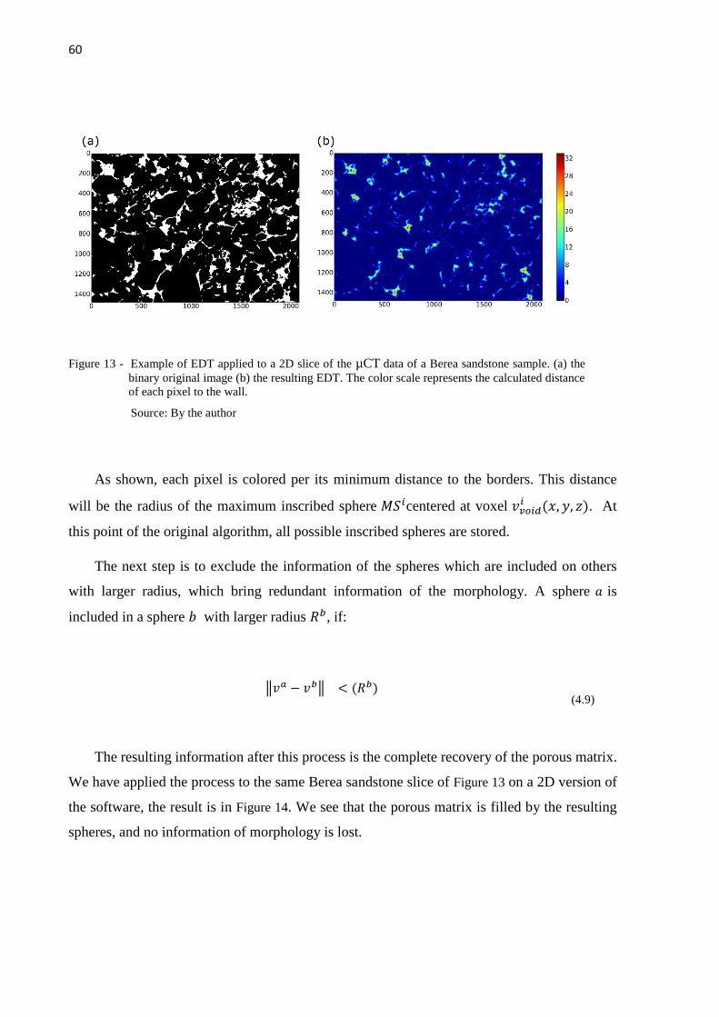
60
Figure 13 - Example of EDT applied to a 2D slice of the µCT data of a Berea sandstone sample. (a) the
binary original image (b) the resulting EDT. The color scale represents the calculated distance
of each pixel to the wall.
Source: By the author
As shown, each pixel is colored per its minimum distance to the borders. This distance
will be the radius of the maximum inscribed sphere 𝑀𝑆𝑖centered at voxel 𝑣𝑣𝑜𝑖𝑑𝑖 (𝑥, 𝑦, 𝑧). At
this point of the original algorithm, all possible inscribed spheres are stored.
The next step is to exclude the information of the spheres which are included on others
with larger radius, which bring redundant information of the morphology. A sphere 𝑎 is
included in a sphere 𝑏 with larger radius 𝑅𝑏, if:
‖𝑣𝑎 − 𝑣𝑏‖ < (𝑅𝑏) (4.9)
The resulting information after this process is the complete recovery of the porous matrix.
We have applied the process to the same Berea sandstone slice of Figure 13 on a 2D version of
the software, the result is in Figure 14. We see that the porous matrix is filled by the resulting
spheres, and no information of morphology is lost.

61
Figure 14 - Final network of spheres. (a) the original distance transform of the image. (b) the maximum spheres
found on the image.
Source: By the author
The final step of the original MS algorithm is the definition of pores and throats. This is
done by ordering the remaining spheres per their radius in descending order and checking the
connection between spheres. Even though the algorithm eliminates spheres which are
included in others with larger radius, it still allows spheres to touch under the limit imposed
by equation (4.9).
Figure 15 - The construction of the network of regions. Two separate networks are constructed: a network
composed of the complete set of spheres (middle image) and a second one composed only of the
medial axis spheres (right image).
Source: By the author
The developed software finds the spheres’ connections and builds a weighted network, in
which the node locations are the spheres’ centers and to each edge is assigned a maximum

62
flow capacity (Figure 15). For each sphere pair, we consider that the maximum possible flow
from sphere i to a neighboring sphere i+1 can be approximated by the area of the cross
section of the adjoining regions (Figure 16).
The capacity of each edge is defined as:
𝐶𝑎𝑝𝑎𝑐𝑖𝑡𝑦(𝑒𝑖,𝑖+1) = 𝜋𝑅𝑐𝑠2
(4.10)
with 𝑅𝑐𝑠 being given by:
𝑅𝑐𝑠 = (𝑅𝑖 − 𝑅𝑖+1
𝑑) (𝑑 − 𝑅𝑖+1) + 𝑅𝑖 (4.11)
where 𝑅𝑖 > 𝑅𝑖+1 are the spheres’ radius and d is the distance between the spheres’
centers.
The final network stores in each node the sphere’s center position, the original sphere’s
radius and the capacities assigned to each edge. This way, the original spheres can be
reconstructed and visualized.
Figure 16 - The model used for the capacity assigned to each edge of the graph. The edge’s capacity of node i to
i+1 will be the area of the full blue circle on the image, given by equation (4.10).
Source: By the author
After the complete regions network is constructed, a medial axis network can be
extracted using the topology of the complete network. This is done by applying the throat

63
concept in the original MS algorithm. When a throat sphere is found, this signals that a path
between two pores exists. To find the medial axis, we search for the shortest path between the
two pore nodes by defining the shortest path as the path that will offer the least resistance for
fluid flow. So, we set the weight of each edge as:
𝑤𝑒𝑖𝑔ℎ𝑡(𝑒𝑖,𝑖+1) =1
𝐶𝑎𝑝𝑎𝑐𝑖𝑡𝑦(𝑒𝑖,𝑖+1)=
1
𝜋𝑅𝑐𝑠2 (4.12)
Then, the shortest path is found through Dijkstra's algorithm81
that searches for the path
of minimum length based on the edges’ weight. An 2D example of both networks are shown
on Figure 17.
Figure 17 - Example of the two networks constructed on the 2D slice of the µCT data of a Berea sandstone
sample. On the left is the complete network, and on the right the medial axis network. The spheres of
the medial axis network are the spheres considered as pores in the algorithm, and the cylinder edges
are the path found between the pores.
Source: By the author
We see that by defining the shortest path as the path of least fluid flow resistance, the
path will be composed by the largest possible spheres. By setting a path connecting these
spheres’ centers, it will follow the medial axis of the object. This way, we recover the
sample’s topology without having to treat the problem of over-branching of the
skeletonization of the sample.

64
A comparison between applying directly the skeletonization procedure through erosion
and the network method is shown on Figure 18. We have enumerated 1-5 examples of over-
branching of the medium that is remedied by our method. We see that the spheres represent a
single pore as being a region of largest volume, as it was proposed before, and the edges
capture the tortuosity of the path between pores as it was expected.
However, one of the limitations of this simple method is pointed out by branching 6. If
multiple paths between two pores exists, only the least resistance path will be considered. To
get all possible paths, a “path removal” approach can be applied. If a path is found, it is
removed from the original network and the algorithm tries to find another path. This is costly
computationally. Another solution would be to enforce the throat node to be a part of the path.
The problem with this approach is that the throat node may not be representative of the medial
axis.
Figure 18 - Comparison of the network shortest path and the skeletonization procedure for finding the medial
axis. 1-5 are examples of the over-branching problem mentioned before of the erosion procedure
(grey lines). 6- limitation of finding one single pathway between pore nodes.
Source: By the author
Another clear advantage of using the network approach is demonstrated on Figure 19. (a)
showns our result by using the shortest path method. Both pore locations and path tortuosity
are captured. (b) showns a pore-throat network acquired by a commercial software. The edges
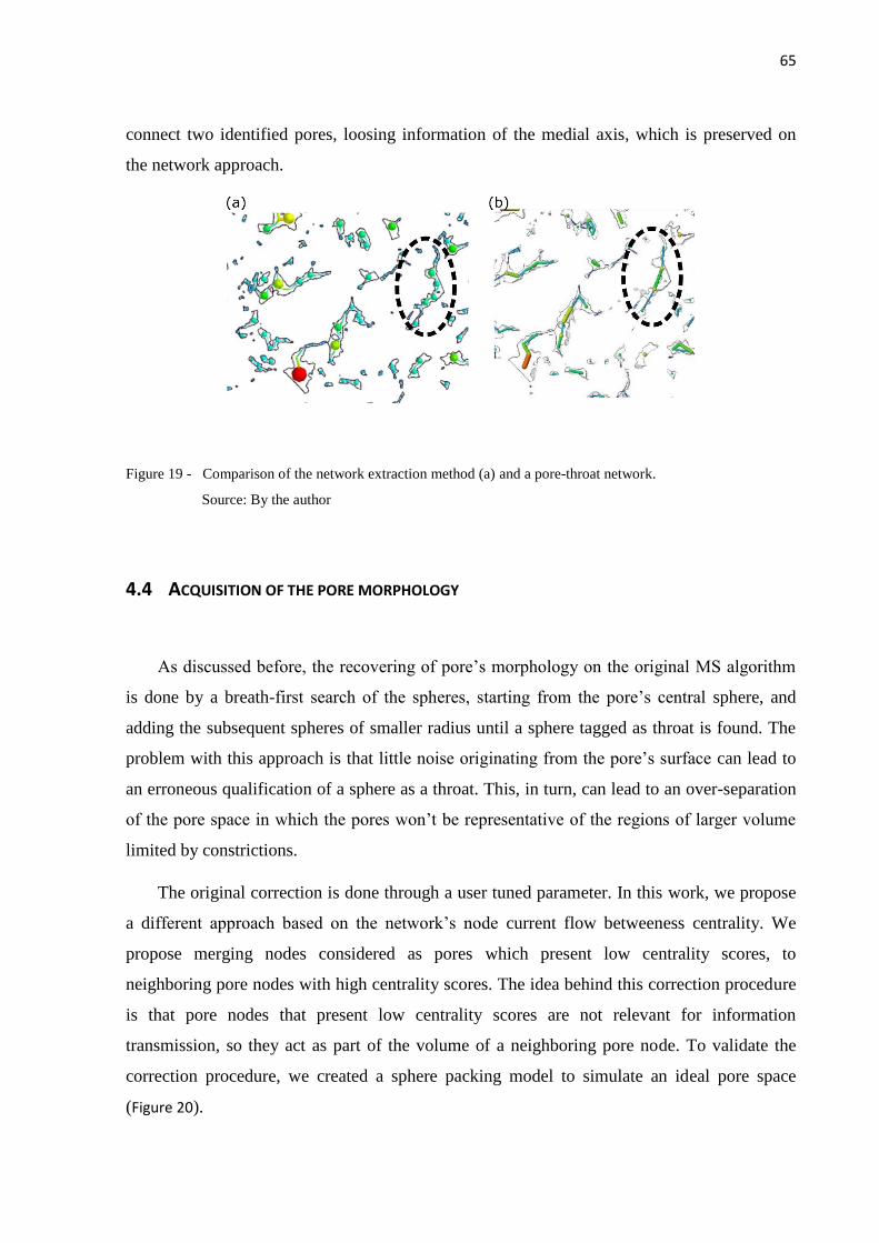
65
connect two identified pores, loosing information of the medial axis, which is preserved on
the network approach.
Figure 19 - Comparison of the network extraction method (a) and a pore-throat network.
Source: By the author
4.4 ACQUISITION OF THE PORE MORPHOLOGY
As discussed before, the recovering of pore’s morphology on the original MS algorithm
is done by a breath-first search of the spheres, starting from the pore’s central sphere, and
adding the subsequent spheres of smaller radius until a sphere tagged as throat is found. The
problem with this approach is that little noise originating from the pore’s surface can lead to
an erroneous qualification of a sphere as a throat. This, in turn, can lead to an over-separation
of the pore space in which the pores won’t be representative of the regions of larger volume
limited by constrictions.
The original correction is done through a user tuned parameter. In this work, we propose
a different approach based on the network’s node current flow betweeness centrality. We
propose merging nodes considered as pores which present low centrality scores, to
neighboring pore nodes with high centrality scores. The idea behind this correction procedure
is that pore nodes that present low centrality scores are not relevant for information
transmission, so they act as part of the volume of a neighboring pore node. To validate the
correction procedure, we created a sphere packing model to simulate an ideal pore space
(Figure 20).

66
Figure 20 - Simulated pore space considered for first pore morphology tests. The medium is an ideal sphere
packing of spheres of equal radius. To simulate a fully connected pore space the spheres are separated
by two voxels from each other. (a) sphere packing wih sphere radius of 30 voxels (b) cross section of
the packing. (c) pore space formed. (d) complete sphere’s network acquired from the space.
Source: By the author
The simulated pore space and the measured centralities based on current flow are shown
on Figure 21. The current flow centrality measure was chosen for its precision, compared to
other centralities measures, as we discussed in the previous chapter. Since the pore nodes are
highly connected, as it was expected, they presented higher centrality than the rest of the
nodes.
Figure 21 - Comparison of the centralities scores for each node type: pore nodes, throat nodes and other nodes in
the network. (a) a visualization of the complete network each node color represents its centrality
value. (b) normalized distributions of centralities of each node group (black other nodes, blue throat
nodes and red pore nodes)
Source: By the author
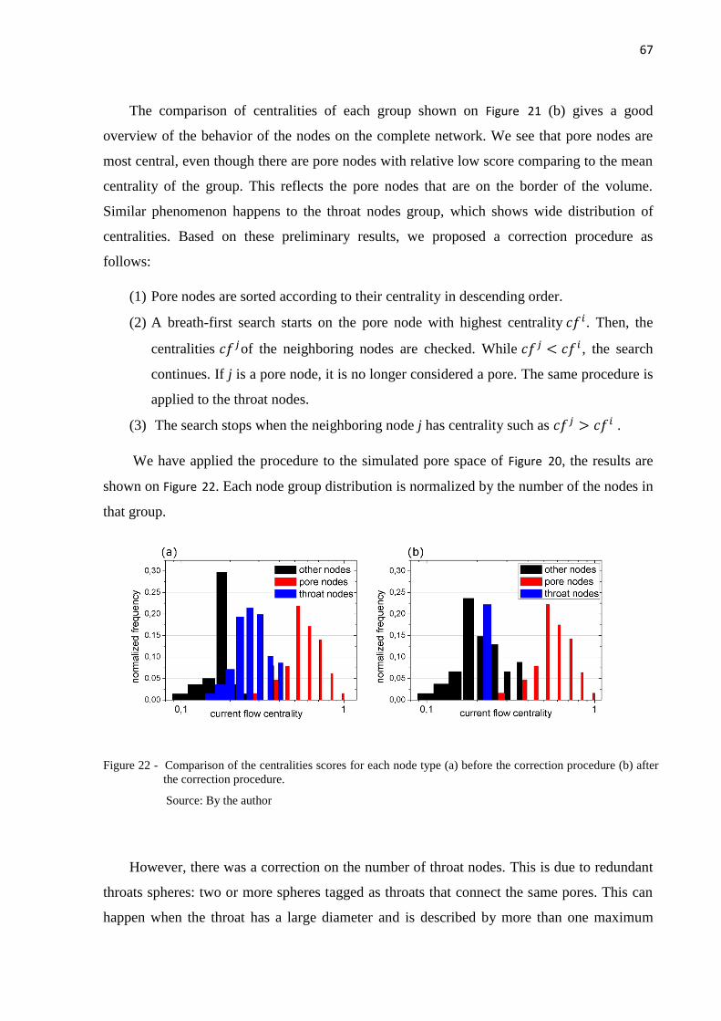
67
The comparison of centralities of each group shown on Figure 21 (b) gives a good
overview of the behavior of the nodes on the complete network. We see that pore nodes are
most central, even though there are pore nodes with relative low score comparing to the mean
centrality of the group. This reflects the pore nodes that are on the border of the volume.
Similar phenomenon happens to the throat nodes group, which shows wide distribution of
centralities. Based on these preliminary results, we proposed a correction procedure as
follows:
(1) Pore nodes are sorted according to their centrality in descending order.
(2) A breath-first search starts on the pore node with highest centrality 𝑐𝑓𝑖. Then, the
centralities 𝑐𝑓𝑗of the neighboring nodes are checked. While 𝑐𝑓𝑗 < 𝑐𝑓𝑖 , the search
continues. If j is a pore node, it is no longer considered a pore. The same procedure is
applied to the throat nodes.
(3) The search stops when the neighboring node j has centrality such as 𝑐𝑓𝑗 > 𝑐𝑓𝑖 .
We have applied the procedure to the simulated pore space of Figure 20, the results are
shown on Figure 22. Each node group distribution is normalized by the number of the nodes in
that group.
Figure 22 - Comparison of the centralities scores for each node type (a) before the correction procedure (b) after
the correction procedure.
Source: By the author
However, there was a correction on the number of throat nodes. This is due to redundant
throats spheres: two or more spheres tagged as throats that connect the same pores. This can
happen when the throat has a large diameter and is described by more than one maximum

68
sphere. The algorithm removes this redundant information by removing the throat spheres
with low centrality.
After the correction procedure is done, the pore’s morphology is recovered by a region-
growing technique starting on the remaining pore nodes. We use these as “seeds” for the
region growing algorithm. Each pore node adds to its body its neighbors interactively. The
procedure stops when no more spheres can be added, or a high centrality throat is found.
We have applied to the simple pore space of Figure 20. Since it is an ideal sphere packing
space, we can have an analytical solution for each pore’s volume.
Figure 23 - The expected equivalent volume V of the pores is the volume of the darker region of the figure.
Source: By the author
Since the grains are composed of spheres of same radius, the volume of the largest space
between the spheres will be the form based on Figure 23:
𝑉𝑝𝑜𝑟𝑒 = 𝑉𝑐𝑢𝑏𝑒 − 𝑉𝑠𝑝ℎ𝑒𝑟𝑒
(4.13)
If we consider a sphere of radius 𝑅𝑒𝑞, such as the sphere’s volume equals 𝑉𝑝𝑜𝑟𝑒, we have:
4
3𝜋𝑅𝑒𝑞
3 = (2𝑅)3 −4
3𝜋𝑅3
(4.14)
So,
𝑅𝑒𝑞 ≅ 0.96𝑅
(4.15)

69
This will be the expected equivalent radius of the pores. Using the case of Figure 20, in which the
sphere’s radius R=30 voxels, the expected equivalent radius of the separated pores will be 𝑅𝑒𝑞 ≅
28.8 𝑣𝑜𝑥𝑒𝑙𝑠 .
Figure 24 - Results for the sphere packing of Figure 20. (a) the pore space separation acquired through the
developed method. (b)The equivalent radius distribution of the pores.
Source: By the author
The results are presented on Figure 24. The image on (a) is a representation of the
separated pores, each pore is the cluster of spheres with the same random color. We see on (b)
that the distribution of pore radius is close to the expected value, with some variations due to
the discrete characteristic of the volume. These are mainly due to the volume’s borders. We
have applied the same method to other sphere packing examples of Figure 25, with expected
equivalent radius of 48 voxels (sphere radius of 50 voxels), 24 voxels sphere radius of 25
voxels) and a mixture of 9.6 and 24 voxels (sphere radius of 10 and 25 voxels respectively).

70
Figure 25 - Simulated ideal sphere packing examples. Left, spheres with R=50, middle R=25 and right a mixture
of small and large spheres: R=10 and R=25.
Source: By the author
We see that the expected pore sizes were recovered correctly from all examples we
applied the algorithm to. The mixture example was assembled such as we had 200 small
spheres and 20 larger spheres, which reflected on the number of smaller pores in comparison
to larger ones (see Figure 25 histograms). The radius variations due to the volume’s borders
are pointed as transition regions, same as the transition from the larger spheres to smaller
spheres in the mixture example. These preliminary results show the method can acquire the
pore’s morphology with good reliability.
Finally, after the correction procedure is done, a pore-throat network is constructed based
on the remaining pore’s center position. To better account for the samples morphology, we
use the medial axis network to find the tortuosity and mean diameter of the paths between
pores to set the capacity parameter of our final network such as:
𝑐𝑎𝑝𝑎𝑐𝑖𝑡𝑦(𝑒𝑖,𝑖+1) =⟨𝐴𝑡ℎ𝑟𝑜𝑎𝑡⟩
𝜏 (4.16)

71
Where ⟨𝐴𝑡ℎ𝑟𝑜𝑎𝑡⟩ is the average cross section area of the throat connecting pore’s i and
i+1 and 𝜏 is the tortuosity of the path. The idea is to account for the morphological variables
that will give the connection between the morphology of the medium and the observed
permeability and formation factor experiments. The final pore-throat network for the first
example is shown on Figure 26
Figure 26 - Pore-throat network extracted from the sphere packing example with R=25. Spheres represent the pore
locations, and the channels represent the throats. The throat’s diameter for all connections is 25
voxels.
Source: By the author


73
5 RESULTS
5.1 APPLICATION ON ROCK SAMPLES
The network extraction method was applied to the three-different porosity and origin
samples: Berea sandstone, Estaillades carbonate and the syntherized sphere packing ( Figure
27).
Figure 27 - Samples used for the pore network extraction method and analysis. (a)-(c) Reconstructed volume and
dimensions of the Berea Sandstone, Estaillades carbonate and syntherized sphere packing samples.
(e)-(f) visualization of the pore space for the Berea, Estaillades and sphere packing samples. All
images were obtained by the developed software, using python mayavi.mlab library.
Source: By the author
The volumetric images were first pre-processed and binarized (with the exception of the
Estaillades sample which was obtained already binarized.). Then, the data was input to the
developed software, and the space was subdivided into sphere’s cells. The output of the
software at this stage is the complete network of spheres cells and the medial axis network of
each sample.

74
Table 2 - Pore-space morphological data from the samples. Samples’ porosity , the pore space surface area S
and volume V, and the specific surface area SSA (surface area per solid volume).
𝝓 𝑺 𝑽 𝑺𝑺𝑨 Berea 0.18 72 mm
2 0.6 mm
3 25 mm
-1
Estaillades 0.13 83 mm2
1.3 mm3
10 mm-1
Spheres 0.35 79 mm2
2.3 mm3
18 mm-1
Source: By the author.
The process was partially parallelized by using the SCOOP parallel library for python
and run on a DELL PWS TOWER 7910. The computational time needed to get the complete
network of spheres and the medial axis network varied between 1h30m for the Berea sample
and 3h for the sphere packing sample. The porosity percentage of the samples escalates the
processing time, according to the resolution of the captured µCT. The complete network of
sphere’s cells of each sample is shown on Figure 28.
Figure 28 - Complete sphere cells networks for the three porous samples: Berea Sandstone, Estaillades carbonate
and the syntherized glass sphere packing. The results show that the division of the pore space into
sphere cells is coherent with the pore-space of each sample.
Source: By the author
The pore-space division into sphere cells eliminated a great portion of the required
information for the characterization of the pore-space, as we can see on Table 3. Since the
sphere cells are allowed to overlap, the distance between nodes are usually smaller than the
sphere’s radius, as we see on the graph of Figure 28. It is interesting to note that the mean
sphere-cell distance is small, 20µm, and it is independent on the sample. However, for the
larger pore-space volume samples Estaillades and Sphere packing, the distance between nodes
can get to 100 µm.

75
The radius of the sphere cells varies according to the sample’s pore-space volume, the
percentage of spheres obeying an exponential decay with the sphere’s radius. The sphere-
packing presented the cells with larger radius, characteristic of its formation, which relates to
larger pore sizes. The Estaillades carbonate presented larger cells than the Berea sample, even
though its total porosity is smaller, signaling that the pore size distribution may be more
correlated to the total pore-space volume than to the sample’s porosity.
Table 3 - Comparison between the total number of pore-space voxels and the total number of nodes of each
sample’s network.
voxels Nodes Berea 18.002.989 205.164
Estaillades 35.517.594 290.727
Spheres 67.785.996 533.766
Source: By the author.
Next, the medial axis network for each of the samples was evaluated, the results
presented on Figure 29. As we can see, the distance between sphere cells differ greatly from
the complete network. The reason for this is that intermediate cells between the medial axis
spheres were removed, leaving just the longest connection between the remaining sphere
cells. The range of the radius distributions of the cells remained the same, just varying in
proportion to the complete network. This means that the medial axis cross section variation is
within the entire range of the complete network sphere cell’s radius.
Figure 29 - Medial axis networks for the three porous samples: Berea Sandstone, Estaillades carbonate and the
syntherized glass sphere packing.
Source: By the author
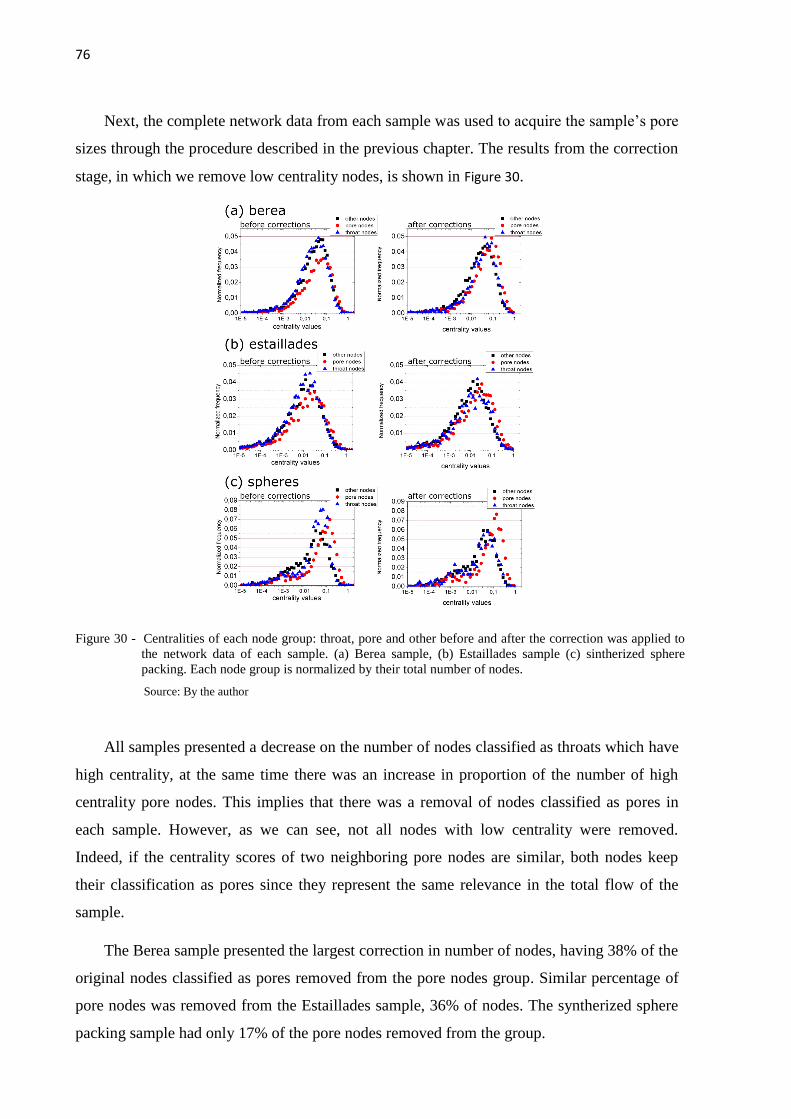
76
Next, the complete network data from each sample was used to acquire the sample’s pore
sizes through the procedure described in the previous chapter. The results from the correction
stage, in which we remove low centrality nodes, is shown in Figure 30.
Figure 30 - Centralities of each node group: throat, pore and other before and after the correction was applied to
the network data of each sample. (a) Berea sample, (b) Estaillades sample (c) sintherized sphere
packing. Each node group is normalized by their total number of nodes.
Source: By the author
All samples presented a decrease on the number of nodes classified as throats which have
high centrality, at the same time there was an increase in proportion of the number of high
centrality pore nodes. This implies that there was a removal of nodes classified as pores in
each sample. However, as we can see, not all nodes with low centrality were removed.
Indeed, if the centrality scores of two neighboring pore nodes are similar, both nodes keep
their classification as pores since they represent the same relevance in the total flow of the
sample.
The Berea sample presented the largest correction in number of nodes, having 38% of the
original nodes classified as pores removed from the pore nodes group. Similar percentage of
pore nodes was removed from the Estaillades sample, 36% of nodes. The syntherized sphere
packing sample had only 17% of the pore nodes removed from the group.
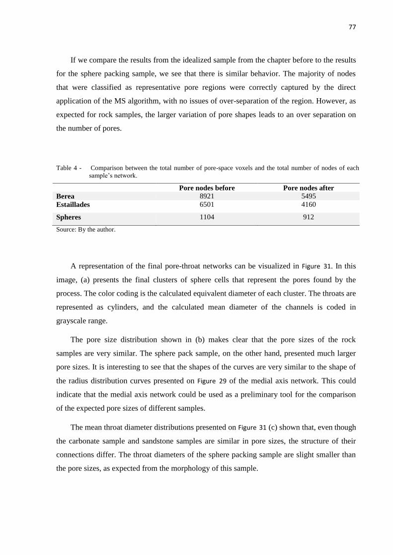
77
If we compare the results from the idealized sample from the chapter before to the results
for the sphere packing sample, we see that there is similar behavior. The majority of nodes
that were classified as representative pore regions were correctly captured by the direct
application of the MS algorithm, with no issues of over-separation of the region. However, as
expected for rock samples, the larger variation of pore shapes leads to an over separation on
the number of pores.
Table 4 - Comparison between the total number of pore-space voxels and the total number of nodes of each
sample’s network.
Pore nodes before Pore nodes after
Berea 8921 5495
Estaillades 6501 4160
Spheres 1104 912
Source: By the author.
A representation of the final pore-throat networks can be visualized in Figure 31. In this
image, (a) presents the final clusters of sphere cells that represent the pores found by the
process. The color coding is the calculated equivalent diameter of each cluster. The throats are
represented as cylinders, and the calculated mean diameter of the channels is coded in
grayscale range.
The pore size distribution shown in (b) makes clear that the pore sizes of the rock
samples are very similar. The sphere pack sample, on the other hand, presented much larger
pore sizes. It is interesting to see that the shapes of the curves are very similar to the shape of
the radius distribution curves presented on Figure 29 of the medial axis network. This could
indicate that the medial axis network could be used as a preliminary tool for the comparison
of the expected pore sizes of different samples.
The mean throat diameter distributions presented on Figure 31 (c) shown that, even though
the carbonate sample and sandstone samples are similar in pore sizes, the structure of their
connections differ. The throat diameters of the sphere packing sample are slight smaller than
the pore sizes, as expected from the morphology of this sample.
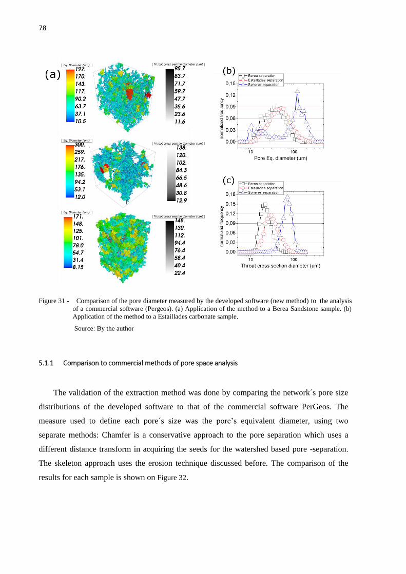
78
Figure 31 - Comparison of the pore diameter measured by the developed software (new method) to the analysis
of a commercial software (Pergeos). (a) Application of the method to a Berea Sandstone sample. (b)
Application of the method to a Estaillades carbonate sample.
Source: By the author
5.1.1 Comparison to commercial methods of pore space analysis
The validation of the extraction method was done by comparing the network´s pore size
distributions of the developed software to that of the commercial software PerGeos. The
measure used to define each pore´s size was the pore’s equivalent diameter, using two
separate methods: Chamfer is a conservative approach to the pore separation which uses a
different distance transform in acquiring the seeds for the watershed based pore -separation.
The skeleton approach uses the erosion technique discussed before. The comparison of the
results for each sample is shown on Figure 32.
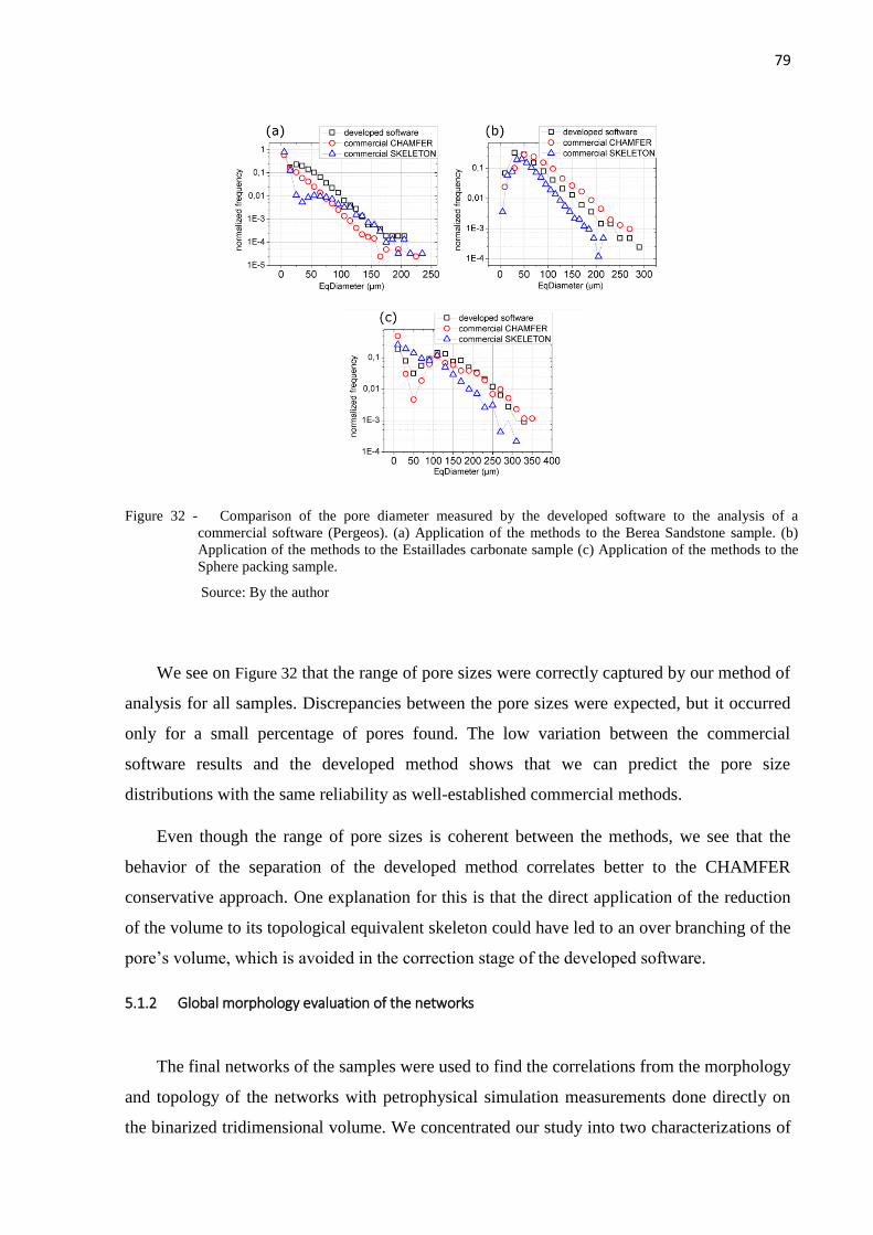
79
Figure 32 - Comparison of the pore diameter measured by the developed software to the analysis of a
commercial software (Pergeos). (a) Application of the methods to the Berea Sandstone sample. (b)
Application of the methods to the Estaillades carbonate sample (c) Application of the methods to the
Sphere packing sample.
Source: By the author
We see on Figure 32 that the range of pore sizes were correctly captured by our method of
analysis for all samples. Discrepancies between the pore sizes were expected, but it occurred
only for a small percentage of pores found. The low variation between the commercial
software results and the developed method shows that we can predict the pore size
distributions with the same reliability as well-established commercial methods.
Even though the range of pore sizes is coherent between the methods, we see that the
behavior of the separation of the developed method correlates better to the CHAMFER
conservative approach. One explanation for this is that the direct application of the reduction
of the volume to its topological equivalent skeleton could have led to an over branching of the
pore’s volume, which is avoided in the correction stage of the developed software.
5.1.2 Global morphology evaluation of the networks
The final networks of the samples were used to find the correlations from the morphology
and topology of the networks with petrophysical simulation measurements done directly on
the binarized tridimensional volume. We concentrated our study into two characterizations of
80
the samples: the resistivity formation factor, and the absolute permeability. The resistivity
Formation Factor was used to characterize the structural measurement of tortuosity through
the medial axis networks, to show an application of the medial axis network directly. We
measured both the geometrical tortuosity and we estimated the electrical tortuosity to see if
the formation factor results were correlated to the tortuosity found through the network
method.
The measurement of the absolute pore space permeability was used in the application of
the separated space. Instead of using the medial axis network, we tested the pore-throat
network in terms of the capacity for flux assigned to each throat. The topology of the final
networks was characterized in terms of connectivity and capacity of flux and these results
compared to the absolute permeability found for each sample.
First the structural analysis will be discussed and then the topological characteristics and
permeability of the samples will be presented.
5.1.3 Structural Analysis
To estimate the samples’ electrical tortuosity, we proposed the following method: pore
nodes presented in each opposing face of the samples were selected as starting and end points
of the possible paths that the flux could follow. To measure the tortuosity of these paths, we
used the definition of tortuosity:
𝜏 =𝐿𝑎(𝑟𝑒𝑎𝑙 𝑝𝑎𝑡ℎ)
𝐿𝑏 (𝑠𝑡𝑟𝑎𝑖𝑔ℎ𝑡 𝑙𝑖𝑛𝑒) (5.1)
The real path (La) was acquired through the application of Dijkstra's algorithm to the
weighted network, which finds the shortest paths between two nodes in a graph. The total
distance of the path is calculated by adding the distance between each node´s (sphere) center,
such as:
𝐿𝑎 = ∑ √(𝑥𝑖 − 𝑥𝑖+1)2 + (𝑦𝑖 − 𝑦𝑖+1)2 + (𝑧𝑖 − 𝑧𝑖+1)2
𝑁𝑎−1
𝑖
(5.2)
Where (𝑥𝑖 , 𝑦𝑖, 𝑧𝑖) is the center position of the ith node, in a path with Na nodes. The
distance Lb is simply the distance between the first and last nodes in the calculated path.
Channels with larger diameter will have higher capacity for flux, this is accounted for in the

81
capacity attribute of the edges of the medial axis networks. So, the closest path will be the
path with least resistance to fluid flow. This is very similar to the definition of the electrical
tortuosity discussed before.
To compare between methods, we also acquired the geometrical tortuosity, simply
defined by the shortest path between the start and ending points. The geometrical tortuosity
was measured on the network not weighted, so all edges were considered to have equal
weight. The distribution of paths’ tortuosity for the weighted network in comparison to the
unweighted is shown on Figure 33.
Figure 33 - Comparison between geometrical and eletrical tortuosity distributions acquired through network
walk. (a)-(c) show the geometrical tortuosity found for the Berea sample, Estaillades sample and
Sphere packing sample respectively. The graphs (d)-(f) show the tortuosity distribution of the paths
considering the diameter of the channels and the mean centrality of the nodes. (d) Berea sample, (e)
Estaillades sample and (f) sphere packing sample.
Source: By the author
The graphs on Figure 33 show that the geometrical tortuosity is always smaller than the
tortuosity found by measurement of paths of least resistance for flux. These results are in
accordance with the experimental results from literature that show that the geometrical
tortuosity tends to be smaller than the electrical tortuosity.

82
Table 5 - Mean path tortuosity results for each direction. Geo stands for the geometrical tortuosity, El. Stands
for the estimated electrical tortuosity.
Direction Berea Geo ⟨𝝉⟩ Berea El.
⟨𝝉⟩ Estaillades Geo
⟨𝝉⟩ Estaillades
El.⟨𝝉⟩ Spheres Geo
⟨𝝉⟩ Spheres El.
⟨𝝉⟩ X 2.3 2.9 2.3 2.8 1.4 1.6
Y 2.4 2.6 2.4 3.6 1.4 1.6
Z 2.0 2.4 2.0 3.2 1.5 1.5
Source: By the author.
Table 5 summarizes the mean tortuosity found for each direction. The mean values found
for the sphere packing and Berea samples of the geometrical tortuosity is very similar to the
mean value found for the estimated electrical tortuosity. This result indicates the homogeneity
of these samples. The carbonate sample, on the other hand, presented a large difference
between methods, the tortuosity of the paths for the estimated electrical tortuosity is much
wider than for the geometrical case. This is coherent with the expected heterogeneity of the
paths of a carbonate in comparison to a sandstone sample.
Figure 34 - Estimated electrical tortuosity distributions in comparison to the porosity profiles of each
sample.(a)-(c) electrical tortuosity distributions for Berea, Estaillades and sphere packing
respectively. The graphs (d)-(f) show the porosity profiles for the Berea, Estaillades and Sphere
packing volumes, respectively.
Source: By the author
The heterogeneity of the samples can also be observed on their porosity profiles (on
Figure 34 d, e and f). We see that the dispersion found for x direction on the tortuosity of the
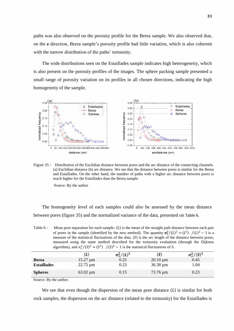
83
paths was also observed on the porosity profile for the Berea sample. We also observed that,
on the z direction, Berea sample’s porosity profile had little variation, which is also coherent
with the narrow distribution of the paths’ tortuosity.
The wide distributions seen on the Estaillades sample indicates high heterogeneity, which
is also present on the porosity profiles of the images. The sphere packing sample presented a
small range of porosity variation on its profiles in all chosen directions, indicating the high
homogeneity of the sample.
Figure 35 - Distribution of the Euclidian distance between pores and the arc distance of the connecting channels.
(a) Euclidian distance (b) arc distance. We see that the distance between pores is similar for the Berea
and Estaillades. On the other hand, the number of paths with a higher arc distance between pores is
much higher for the Estaillades than the Berea sample.
Source: By the author
The homogeneity level of each samples could also be assessed by the mean distance
between pores (figure 35) and the normalized variance of the data, presented on Table 6.
Table 6 - Mean pore separation for each sample: ⟨𝐿⟩ is the mean of the straight path distance between each pair
of pores in the sample (identified by the new method). The quantity 𝝈𝒍𝟐 ⟨𝐿⟩2 =⁄ ⟨𝐿2⟩ ⟨𝐿⟩2 − 1⁄ is a
measure of the statistical fluctuations of the data. ⟨𝑆⟩ is the arc length of the distance between pores,
measured using the same method described for the tortuosity evaluation (through the Dijkstra
algorithm), and 𝜎𝑠2 ⟨𝑆⟩2 =⁄ ⟨𝑆2⟩ ⟨𝑆⟩2 − 1⁄ is the statistical fluctuations of S.
⟨𝑳⟩ 𝝈𝑳𝟐 ⟨𝑳⟩𝟐⁄ ⟨𝑺⟩ 𝝈𝒔
𝟐 ⟨𝑺⟩𝟐⁄ Berea 15.27 µm 0.25 20.10 µm 0.45 Estaillades 22.75 µm 0.23 36.38 µm 1.04
Spheres 63.02 µm 0.15 73.76 µm 0.23
Source: By the author.
We see that even though the dispersion of the mean pore distance ⟨𝐿⟩ is similar for both
rock samples, the dispersion on the arc distance (related to the tortuosity) for the Estaillades is

84
twice the dispersion for the Berea data. So, even though the pores are distributed in similar
form in the pore space, the path between each pore is, on average, more tortuous on the
Estaillades sample. The opposite could be seen for the sphere packing sample. The dispersion
of both the arc lengths S and real distance L were small, which implies high homogeneity of
the sample.
Figure 36 - Behavior of the tortuosity distributions for each sample in each chosen direction.
Source: By the author
We see from Figure 36 that, in most cases, the path chosen most frequently was the same,
as we can see by the behavior of the distributions. The exceptions were the paths on the x
direction for the Berea sample and the path on the y direction on the Estaillades sample. We
can understand from these results that, in these cases, the probability that the flux will follow
either a tortuous path or a straight path is very similar. This is correlated to an intrinsic
heterogeneity of these samples on these directions.
Since the electrical tortuosity is correlated to the paths in which we have the largest
density of flux, we compared the tortuosity correlated with the highest frequency on the
graphs of Figure 36 to the results for resistive formation factor simulated on Pergeos (Table 7).

85
We see that the direction in which we had largest tortuosity correlates to the formation
factor result on that direction. The Estaillades sample y direction distribution didn’t have a
clear largest frequency, so both the tortuosity related to the largest peak (τ=3.0) and the mean
tortuosity (τ=3.6) is shown.
Table 7 - Tortuosity of paths found more frequently for each direction compared to the Formation Factor results.
Direction Berea
max(τ)
Berea
Formation
Factor
(Pergeos)
Estaillades
max(τ)
Estaillades
Formation
Factor
(Pergeos)
Spheres
max(τ)
Spheres
Formation
Factor
(Pergeos)
x 2.7 41 2.1 88 1.6 4.3
y 2.6 38 3.0-3.6 383 1.5 4.4
z 2.0 18 3.2 263 1.5 4.8
Source: By the author.
We applied the formula (3.9) to estimate the formation factor using the results of
tortuosity from Table 7. The parameter α=2 was used for the rock samples, and α=1 for the
sphere packing sample. For the Estaillades sample, we estimated the cementation factor
m=1.5, using the tortuosity results on the x direction as an adjustment. For the Berea sample
and sphere packing we let m=1.0.
Table 8 - Results for the calculated Formation Factor (NN) of the samples compared to the apparent Formation
Factor acquired with the software PerGeos.
Berea Estaillades Spheres
Direction F (NN) Apparent F
(Pergeos)
X 40,5 41
Y 37,5 38
Z 22 18
Direction F (NN) Apparent F
(Pergeos)
X 94 88
Y 192-276 383
Z 218 263
Direction F (NN) Apparent F
(Pergeos)
X 4.6 4.3
Y 4.3 4.4
Z 4.3 4.8
Source: By the author.
There is good agreement between the simulated formation factor and the estimated values
from the application of (3.9). The homogeneity of the sphere packing sample led to a linear
correlation of tortuosity and the formation factor, as we can see on Table 8 . The results for the
Berea sample were also very close to the expected formation factor value, showing that the
method of using the medial axis networks to estimate the sample’s tortuosity, not simply the
geometric tortuosity, but the electrical tortuosity, leads to coherent results.
The high levels of the apparent formation factor on the y and z directions provided by
for the Estaillades sample are not unusual for carbonate samples.51,63,82-83
This indicates high
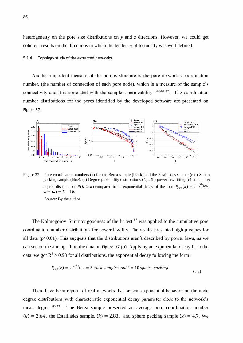
86
heterogeneity on the pore size distributions on y and z directions. However, we could get
coherent results on the directions in which the tendency of tortuosity was well defined.
5.1.4 Topology study of the extracted networks
Another important measure of the porous structure is the pore network’s coordination
number, (the number of connection of each pore node), which is a measure of the sample’s
connectivity and it is correlated with the sample’s permeability 1,61,84–86
. The coordination
number distributions for the pores identified by the developed software are presented on
Figure 37.
Figure 37 - Pore coordination numbers (k) for the Berea sample (black) and the Estaillades sample (red) Sphere
packing sample (blue). (a) Degree probability distributions (𝑘) , (b) power law fitting (c) cumulative
degree distributions 𝑃(𝐾 > 𝑘) compared to an exponential decay of the form 𝑃𝑒𝑥𝑝(𝑘) = 𝑒−(𝑘 ⟨𝑘⟩⁄ )
,
with ⟨𝑘⟩ = 5 − 10.
Source: By the author
The Kolmogorov–Smirnov goodness of the fit test 87
was applied to the cumulative pore
coordination number distributions for power law fits. The results presented high p values for
all data (p>0.01). This suggests that the distributions aren´t described by power laws, as we
can see on the attempt fit to the data on Figure 37 (b). Applying an exponential decay fit to the
data, we got R2 > 0.98 for all distributions, the exponential decay following the form:
𝑃𝑒𝑥𝑝(𝑘) = 𝑒−(𝑘 𝑡⁄ ), 𝑡 = 5 𝑟𝑜𝑐𝑘 𝑠𝑎𝑚𝑝𝑙𝑒𝑠 𝑎𝑛𝑑 𝑡 = 10 𝑠𝑝ℎ𝑒𝑟𝑒 𝑝𝑎𝑐𝑘𝑖𝑛𝑔 (5.3)
There have been reports of real networks that present exponential behavior on the node
degree distributions with characteristic exponential decay parameter close to the network’s
mean degree 88,89
. The Berea sample presented an average pore coordination number
⟨𝑘⟩ = 2.64 , the Estaillades sample, ⟨𝑘⟩ = 2.83, and sphere packing sample ⟨𝑘⟩ = 4.7. We

87
see that the exponential decay parameter is not close to the mean degree of the networks, but
it is correlated = 2 ∗ ⟨𝑘⟩ .
This shows that the mean degree alone may not give enough information on the
networks’ topology, since the variation of connectivity indicates that we find highly
connected nodes with relevant frequency. The exponential behavior instead of a power-law
heavy tail curve for the degree distribution might be associated to the pore distribution in in
the tridimensional space. This gives a low probability of long range connections.
The mean connectivity reported in the literature for Berea samples is ⟨𝑘⟩~3 and for
Estaillades samples ⟨𝑘⟩ ~ 2.8 51,80
One explanation for the lower values found in the extracted
networks are the pore nodes on the border of the volumes. These pores present k=1, leading to
an unrealistic low connectivity. After eliminating these pores from the distributions of the
rock samples, the average connectivity found was ⟨𝑘⟩ ~ 3.14 for the Berea sample and
⟨𝑘⟩ ~ 2.9 for the Estaillades sample, which is in agreement with values from the literature.
We compared the mean values of connectivity with the mean permeability found by
direct simulation on the pore space volume using the commercial software Pergeos. The
results are summarized on Table 9. We see that mean absolute permeability found in the
simulations is highest for the sphere packing, which presented the highest mean coordination
number as well. We had a slight difference in permeability between the carbonate and
sandstone samples, which agrees to the mean connectivity found in the proposed network
model.
Table 9 - Mean absolute permeability ⟨𝑝⟩ , simulated on the binary data using the commercial software
Pergeos, in comparison with the mean connectivity ⟨𝑘⟩ calculated in the network model.
Samples ⟨𝒑⟩ µ𝐦𝟐 ⟨𝒌⟩ Berea 2.14 3.14
Estaillades 1.69 2.9
Spheres 120.2 4.7
Source: By the author.
The absolute permeabilities of the samples were also compared to the flow capacity of
the pore-throat networks models. We choose to evaluate the absolute permeability on Z
direction, in which the distinction of the absolute values found on the simulations for each
sample were more evident. The total flow capacity of each sample was acquired by finding
the paths of maximum flow, setting a super source of flow connected to the pores nodes in the
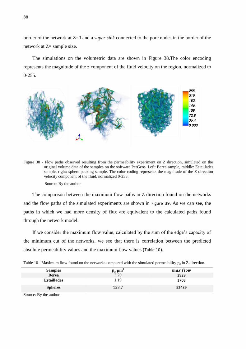
88
border of the network at Z=0 and a super sink connected to the pore nodes in the border of the
network at Z= sample size.
The simulations on the volumetric data are shown in Figure 38.The color encoding
represents the magnitude of the z component of the fluid velocity on the region, normalized to
0-255.
Figure 38 - Flow paths observed resulting from the permeability experiment on Z direction, simulated on the
original volume data of the samples on the software PerGeos. Left: Berea sample, middle: Estaillades
sample, right: sphere packing sample. The color coding represents the magnitude of the Z direction
velocity component of the fluid, normalized 0-255.
Source: By the author
The comparison between the maximum flow paths in Z direction found on the networks
and the flow paths of the simulated experiments are shown in Figure 39. As we can see, the
paths in which we had more density of flux are equivalent to the calculated paths found
through the network model.
If we consider the maximum flow value, calculated by the sum of the edge’s capacity of
the minimum cut of the networks, we see that there is correlation between the predicted
absolute permeability values and the maximum flow values (Table 10).
Table 10 - Maximum flow found on the networks compared with the simulated permeability 𝑝𝑧 in Z direction.
Samples 𝒑𝒛 µm2 𝒎𝒂𝒙 𝒇𝒍𝒐𝒘
Berea 3.20 2929 Estaillades 1.19 1708
Spheres 123.7 52489
Source: By the author.

89
This is good evidence that the network model is able to capture the morphology of the
channels without critical loss of information from the volume data.
Figure 39 - Flow paths from the simulated permeability experiment on the complete volume, and the network
maximum flow paths found for each sample. 1: the network color coded according the the edge’s
total flow capacity. 2- the network color coded according to the used capacity of each edge. 3:
simulated permeability experiment (PERGEOS). The spheres represent the inlet and outlet points
used for the max flow calculations on the networks. (a) Berea sample, (b) Estaillades sample and (c)
Sphere packing sample.
Source: By the author
We also see that the throats’ morphology changes significantly the topology of the
networks. We measured both the current flow centrality distributions and closeness centrality
distributions. The current flow betweenness centrality distributions remained with the same
shape if we considered the weighted networks or unweighted networks, with a slight increase
of the percentage of nodes with higher score (Figure 40).

90
Figure 40 - Comparison of the current flow betwenness centrality distributiona of the networks without
considering the edge weights (A) and considering the edge weights (B). We have a slight increase of
higher centrality nodes.
Source: By the author
However, the change in topology between the weighted and unweighted networks were
evident on the closeness centrality scores of the nodes. The results from Figure 41 show that, if
we consider the pore positioning on the network without taking into account the diameter and
tortuosity of the connecting channels, the mean distance between nodes increases, given by
the relative percentage of nodes that presented low closeness centrality.
This is especially true for the Estaillades sample. We see that the mean distance between
nodes decreases considerably when we take into account the morphology of the throat
channels. This could indicate that there can be pore nodes acting as bridges between two
different pore clusters.

91
Figure 41 - Comparison of the closeness centrality distribution of the networks without considering the edge
weights ( the distance between nodes is the number of steps in the network) and considering the edge
weights. We see that when we consider the edge weights, the number of nodes with high closeness
centrality tends to increase.
Source: By the author
Even though the results of the closeness centrality distributions could indicate high
heterogeneity on the mean node strength, the measurement of the local entropy shows that the
majority of nodes presented a homogeneous distribution on the distance and arc distances
between pores Figure 42 (c).
The networks also presented a non-trivial correlation between the number of connections
a node has and the mean strength of the nodes. The correlation of the node’s connectivity and
the mean distance between nodes and the total channel length s are shown in Figure 42 (b) and
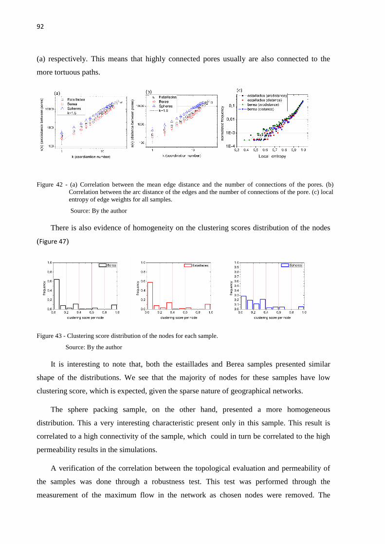
92
(a) respectively. This means that highly connected pores usually are also connected to the
more tortuous paths.
Figure 42 - (a) Correlation between the mean edge distance and the number of connections of the pores. (b)
Correlation between the arc distance of the edges and the number of connections of the pore. (c) local
entropy of edge weights for all samples.
Source: By the author
There is also evidence of homogeneity on the clustering scores distribution of the nodes
(Figure 47)
Figure 43 - Clustering score distribution of the nodes for each sample.
Source: By the author
It is interesting to note that, both the estaillades and Berea samples presented similar
shape of the distributions. We see that the majority of nodes for these samples have low
clustering score, which is expected, given the sparse nature of geographical networks.
The sphere packing sample, on the other hand, presented a more homogeneous
distribution. This a very interesting characteristic present only in this sample. This result is
correlated to a high connectivity of the sample, which could in turn be correlated to the high
permeability results in the simulations.
A verification of the correlation between the topological evaluation and permeability of
the samples was done through a robustness test. This test was performed through the
measurement of the maximum flow in the network as chosen nodes were removed. The

93
choice methods were: nodes with high closeness centrality scores, nodes with high current
flow betweenness centrality scores, largest pore nodes and finally through a targeted edge
removal, removing edges with high capacity.
Table 11 - Number of nodes removed to interrupt flow through closeness centrality targeted attack
sample % nodes removed Berea 0.02
Estaillades 0.09
Spheres 1.50
Source: By the author.
What we observed is that the closeness centrality of the nodes (Table 11) is that, indeed,
nodes with higher closeness centrality play a major part on the flow. The results from Table 11
show that very small percentage of node needed to be removed such that the flow was
interrupted.
A different result was observed when we targeted the edges with high capacity. As we
can see on Figure 44, the distribution of the edges capacity is very heterogeneous for the rock
cores.
Figure 44 - Edge capacity distribution of each sample. We see that for the estaillades and Berea samples, a
majority of nodes presented edges with low capacity. The Sphere packing sample presented, on the
other hand, a more homogeneous distribution.
Source: By the author
The homogeneity of the sphere packing sample is evident, on the other hand. However,
even if the edges capacity distribution is heterogeneous for the Berea sample, the directed
attack was not as efficient on interrupting flow as it was when choosing nodes with high
closeness centralities.
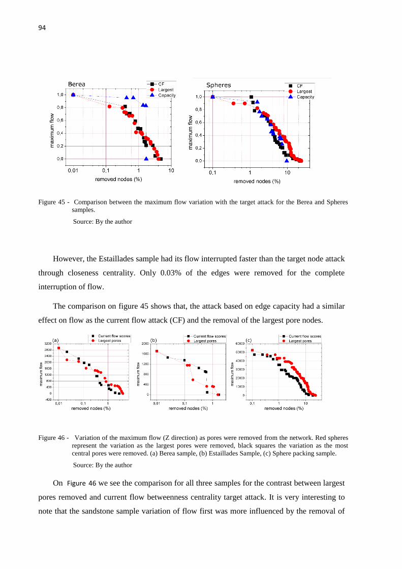
94
Figure 45 - Comparison between the maximum flow variation with the target attack for the Berea and Spheres
samples.
Source: By the author
However, the Estaillades sample had its flow interrupted faster than the target node attack
through closeness centrality. Only 0.03% of the edges were removed for the complete
interruption of flow.
The comparison on figure 45 shows that, the attack based on edge capacity had a similar
effect on flow as the current flow attack (CF) and the removal of the largest pore nodes.
Figure 46 - Variation of the maximum flow (Z direction) as pores were removed from the network. Red spheres
represent the variation as the largest pores were removed, black squares the variation as the most
central pores were removed. (a) Berea sample, (b) Estaillades Sample, (c) Sphere packing sample.
Source: By the author
On Figure 46 we see the comparison for all three samples for the contrast between largest
pores removed and current flow betweenness centrality target attack. It is very interesting to
note that the sandstone sample variation of flow first was more influenced by the removal of

95
the largest pores, and then by the highly connected pores. The Estaillades sample, in the other
hand, is more dependent on larger pores for the fluid flow, as we can see on Figure 46 (b).
The sphere packing sample showed that the high homogeneity on pore sizes makes the
network more dependent on the highly connected nodes. Even though the size of pores is
large, the centrality of the pores is more relevant for the connectivity of the sample.
5.2 APPLICATION ON ACIDIFICATION SAMPLES - WORMHOLES
On the acidification samples, the study aimed at the characterization of the final
morphology of the channels (wormholes) formed after the acidification process. The µCT
data from the samples contained the original pore space and the wormhole, so, to focus only
on the wormholes, first we processed the volume to find the largest connected region which
percolated in the direction of the acidification. The characteristics of the samples after this
process are on Table 12.
Table 12 - Characteristics of µCT data of the wormhole samples. Resolution, number of images slices, volume
of the selected wormhole, surface area of the selected wormhole and the porosity 𝝓 of the sample
considering only the wormhole.
Sample name
Resolution (µm)
N slices Sample Volume
(cm3)
Wormhole Volume (cm3)
Wormhole Surface
Area(cm2)
𝝓 (%)
E2 42.7 (775x775)x1500 85 1.8 5.8 2.1
E4 45.2 (775x775)x1500 85 1.3 6.7 1.5
E5 45.2 (775x775)x1500 85 2.3 17.7 2.7
E8 45.2 (775x775)x1500 85 1.3 3.5 1.5
E9 45.2 (775x775)x1500 85 3.1 22.6 3.6 Source: By the author.
The surface of the structures formed from the acidification procedure can be visualized
in Figure 47. As we can see from the data in Table 12, sample E9 presented the largest surface
area, follow by sample E5. These two samples differ greatly from the E2, E4 and E8 samples,
which presented more structured channels.
Table 13 - Porosity 𝝓 and absolute permeability of the samples previous to the acidification procedure
Sample name 𝝓 (%) Absolute permeability (mD)
E2 16.2 >40
E4 15.3 >40
E5 15.4 >40
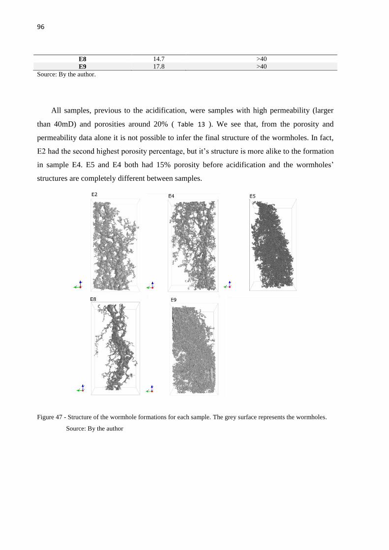
96
E8 14.7 >40
E9 17.8 >40
Source: By the author.
All samples, previous to the acidification, were samples with high permeability (larger
than 40mD) and porosities around 20% ( Table 13 ). We see that, from the porosity and
permeability data alone it is not possible to infer the final structure of the wormholes. In fact,
E2 had the second highest porosity percentage, but it’s structure is more alike to the formation
in sample E4. E5 and E4 both had 15% porosity before acidification and the wormholes’
structures are completely different between samples.
Figure 47 - Structure of the wormhole formations for each sample. The grey surface represents the wormholes.
Source: By the author
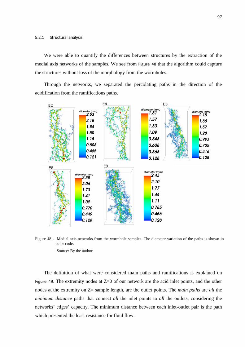
97
5.2.1 Structural analysis
We were able to quantify the differences between structures by the extraction of the
medial axis networks of the samples. We see from Figure 48 that the algorithm could capture
the structures without loss of the morphology from the wormholes.
Through the networks, we separated the percolating paths in the direction of the
acidification from the ramifications paths.
Figure 48 - Medial axis networks from the wormhole samples. The diameter variation of the paths is shown in
color code.
Source: By the author
The definition of what were considered main paths and ramifications is explained on
Figure 49. The extremity nodes at Z=0 of our network are the acid inlet points, and the other
nodes at the extremity on Z= sample length, are the outlet points. The main paths are all the
minimum distance paths that connect all the inlet points to all the outlets, considering the
networks’ edges’ capacity. The minimum distance between each inlet-outlet pair is the path
which presented the least resistance for fluid flow.
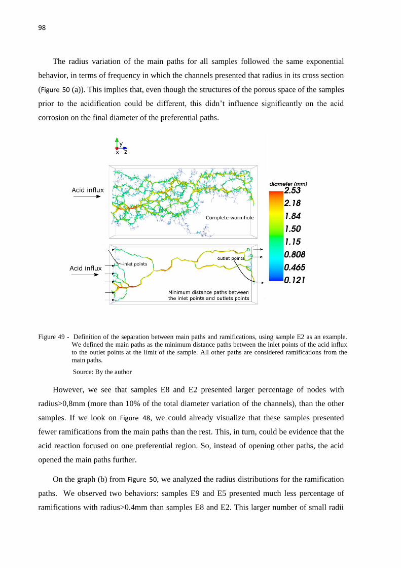
98
The radius variation of the main paths for all samples followed the same exponential
behavior, in terms of frequency in which the channels presented that radius in its cross section
(Figure 50 (a)). This implies that, even though the structures of the porous space of the samples
prior to the acidification could be different, this didn’t influence significantly on the acid
corrosion on the final diameter of the preferential paths.
Figure 49 - Definition of the separation between main paths and ramifications, using sample E2 as an example.
We defined the main paths as the minimum distance paths between the inlet points of the acid influx
to the outlet points at the limit of the sample. All other paths are considered ramifications from the
main paths.
Source: By the author
However, we see that samples E8 and E2 presented larger percentage of nodes with
radius>0,8mm (more than 10% of the total diameter variation of the channels), than the other
samples. If we look on Figure 48, we could already visualize that these samples presented
fewer ramifications from the main paths than the rest. This, in turn, could be evidence that the
acid reaction focused on one preferential region. So, instead of opening other paths, the acid
opened the main paths further.
On the graph (b) from Figure 50, we analyzed the radius distributions for the ramification
paths. We observed two behaviors: samples E9 and E5 presented much less percentage of
ramifications with radius>0.4mm than samples E8 and E2. This larger number of small radii
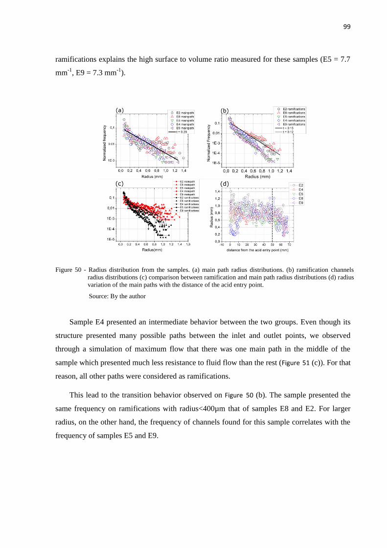
99
ramifications explains the high surface to volume ratio measured for these samples (E5 = 7.7
mm-1
, E9 = 7.3 mm-1
).
Figure 50 - Radius distribution from the samples. (a) main path radius distributions. (b) ramification channels
radius distributions (c) comparison between ramification and main path radius distributions (d) radius
variation of the main paths with the distance of the acid entry point.
Source: By the author
Sample E4 presented an intermediate behavior between the two groups. Even though its
structure presented many possible paths between the inlet and outlet points, we observed
through a simulation of maximum flow that there was one main path in the middle of the
sample which presented much less resistance to fluid flow than the rest (Figure 51 (c)). For that
reason, all other paths were considered as ramifications.
This lead to the transition behavior observed on Figure 50 (b). The sample presented the
same frequency on ramifications with radius<400µm that of samples E8 and E2. For larger
radius, on the other hand, the frequency of channels found for this sample correlates with the
frequency of samples E5 and E9.

100
Figure 51 - Definition of the separation between main paths and ramifications for the E4 sample. (a) complete
sample color coded according to the path’s diameter. (b) main paths selected from the sample, color
coded according to the path’s diameter. (c) maximum flow passage in each edge.
Source: By the author
We can see that, even though the main paths have a much larger diameter in comparison
to the ramifications, we still need many small diameter spheres to represent the paths
completely, as we see on Figure 50 (c): 90% of the spheres representing the main paths are in
the same range as the ramifications. We have two reasons for this: paths smaller in diameter
need a great number of maximum spheres to capture its structure than paths with larger
diameters. The second reason is that the extremities of the samples are composed mainly of
paths with small diameter, which are connected to the main paths.
The method also allowed the measurement of the variation of the diameter of the main
paths on the direction on the acid influx (Figure 50 (d)). Up until the 50mm limit, we have no
discernible correlation of the samples’ z direction length and the diameter of the paths. The
mean radius of the entire sample group measured in this case was 0.7 ± 0.3𝑚𝑚.
We observed that, after the 50mm limit, the main channels’ radii start to decrease. This
could indicate that there is a loss on the effectiveness of the chemical reaction at this point.
The electrical tortuosity of the main paths was also evaluated, with the same process as
we have applied to the rock samples. The inlet and outlet points were chosen on either
extremity on the Z axis of the samples, as it is shown on Figure 49. Then, the lengths of all the

101
possible paths of connection between the outlets and inlets were measured. This resulted on
the tortuosity distributions shown on Figure 52.
We see that most samples presented wide distribution of tortuosity of the paths. Samples
E4 and E9 presented the widest distributions, in which we have paths connecting inlets to the
outlets that are twice as long as the straight line connecting them. This is due to the number of
ramifications that appeared on the acidification process. Sample E5 and E2 presented a
tendency of most paths presenting the same tortuosity (30% of the paths), which means that a
particle will follow the same path 30 percent of the times, independent on the inlet-outlet pair
chosen.
Sample E8 was the only one that presented a small variation on the tortuosity measured.
This shows that the morphology of the wormhole followed basically one main channel, as we
could see already qualitatively by the visualization of the network extracted. This information
could implicate that the flow is entirely dependent on a single channel.
Figure 52 - Tortuosity distributions in the direction of the acidification for each sample.
Source: By the author

102
5.2.2 Morphology evaluation through random walk simulation
Through the tortuosity direct measure, we could assess the morphology of the main paths.
In order to verify the influence of the samples’ ramifications, we proposed a particle diffusion
experiment through random walk. The particles start at a randomly chosen node in the medial
axis network, then at each step the particle can move to a different node or remain on the
current node, with the probability:
𝑝𝑖,𝑗 =𝑐(𝑖, 𝑗)
𝑠(𝑘) (5.4)
Where c(i,j) is the edge’s capacity and s(k) is the total strength of the node. So, there is a
larger probability that a particle will move to nodes with larger diameter. Then, the particles
are allowed to diffuse in the network until one of two things happens: either the particle finds
an outlet node, meaning that the particle was allowed to leave the wormhole, or the simulation
reaches a time limit.
Figure 53 - Mean frequency that a site was visited in the simulations for each sample.
Source: By the author

103
The simulation was run for 10000 events for each sample, and the number of times a
node was visited and the number of different sites that were visited were measured.
The result for each simulation of the visited frequency of the nodes are shown in color
coding in Figure 55. We see that, for this model, there are region of the samples in which the
particles choose more frequently to pass through then others. This is expected since we gave
preference for regions with larger diameter in the simulations. What is interesting to note is
that there are some specific sites that seemed to act as bridges, being visited far more times
than others.
Figure 54 - Percentage of the total unique visited sites versus the simulation time for each sample. Here only the
results of the particles that reached the outlet points in shown.
Source: By the author
The coverage results for the samples shown on Figure 54 gives another view on the
tortuosity results from before. We see, as expected, that the high number of ramifications
present on samples E9 and E5 leads to a need for the particle to, in average, walk a larger
number of steps in order to reach the outlet points. However, we see that the number of
distinct sites visited is not as high as the other samples. So, even though the ramification paths
add a new level of complexity for these samples, the particles tend to follow common paths to
find the outlet points.
104
Table 14 - Compared results of the mean number of steps need to reach the outlet points and the number of
nodes in each network.
Sample name ⟨𝑵𝒔𝒕𝒆𝒑𝒔⟩ Nnodes ⟨𝑵𝒔𝒕𝒆𝒑𝒔⟩/𝑵𝒏𝒐𝒅𝒆𝒔 E2 30498 12420 2.4
E4 31063 10391 2.9
E5 81434 39759 2.0
E8 49924 4490 11.1
E9 98112 65017 1.5 Source: By the author.
Another important result from these simulations concerns sample E4. Sample E4
presented a wide distribution on the tortuosity of its main paths. However, the diffusion
simulations show that, even though the paths are tortuous, they act as shortcuts for the
particles to reach the outlet points. We see this from the results of Table 14. The mean number
of steps needed for a particle to walk from its starting point to the outlets is in average the
same of sample E2, which presented a lower mean tortuosity of the main paths.
This means that, even though the branching on the main paths might lead to wide
distributions on tortuosity, this branching can also be positive if we are interested in the
diffusion of a solute through the region, given that the diameter of the branching channel is
large.
The results from Table 14 for sample E8 also show that the number of steps needed for the
particles to reach the outlet points surpassed the number of nodes in the network. This is a
consequence of the model not being self-exclusive. Since the acidification on this sample
acted on one main channel, the particles didn’t have a preferential pathway to follow. So, the
probability of the particle moving inside the channel or staying put was very similar. We can
make the analogy that the particle acts as it is in free diffusion, instead of restricted by the
morphology of the sample.
5.2.3 Network robustness evaluation
To assess the dependence on the main paths and the dependence on certain regions of our
samples saw on the diffusion simulations, the robustness of the networks was evaluated
similarly as it was done for the rock samples. The variation of the maximum flow in the Z
direction was measured as the nodes of the networks were removed. The inlets and outlets
chosen as it was done in the main paths evaluations. The difference here is that there wasn´t a

105
separation on pore nodes and throats. The nodes to be removed were selected directly from
the medial axis network.
We measured the effectiveness of the centrality measures to find the major throughputs
nodes for fluid flow with the robustness test as well. We have applied the target attack using
page rank, betweenness centrality, current flow betweenness centrality and eigenvector
centrality. We had two interesting results with the current flow betweenness centrality
measures and the eigenvector centrality measures. We saw that the current flow betweenness
centrality was the most efficient centrality measure to find the critical nodes for the continuity
of the flow on the networks.
Figure 55 - Visualization of the current flow centrality scores for each sample.
Source: By the author
The current flow betweenness centrality scores can be visualized on Figure 52. We see
that the regions in which we had high centrality scores correspond to regions of bifurcation of
the paths. Figure 56 (a) shows the variation of the maximum flow measured with the removal
of nodes with high current flow scores. We see that the flow decays fast for all samples,
especially for the E2, E8 and E5. The least effective case was for the E4 sample, but even for

106
this sample, we needed under 1% of the nodes removed for the flow to stop completely.
Comparing to the random case, Figure 56 (c), in which the nodes were chosen randomly for
removal, there was a minimum of 2% of node removal for the maximum flow to fall to half
the initial value, and a minimum of 4% for the flow to stop completely. The random case was
run for 1000 of events.
Figure 56 -Variation of the maximum flow measured with the removal of nodes. (a) nodes were removed
according to the current flow centrality scores. (b) nodes were removed according with its
eigenvector centrality score. (c) nodes were removed randomly (d) comparison of the robustness test
for samples E5,E8 and E9 of the results by current flow scores (black) and eigenvector centrality
scores (red).
Source: By the author
The results of the attack using the eigenvector centrality scores are shown on Figure 56
(b). We see that, for some samples, more specifically E5, E8 and E9, the eigenvector
centrality score was a very efficient measure to find the critical regions for the fluid flow, on
the other hand, for the samples E4 and E2 that wasn’t the case. This points out to two
morphologies found: the wormholes that are dependent on one path for the flow to pass in the
Z direction and the ones that branched into many large diameter paths.
The dependence on one path seemed to be the case for the E8 sample, however E5 and
E9 also presented that behavior, even though we had a large variation of the paths tortuosity
for these samples. We see from Figure 56 (d) that still the current flow centrality scores were
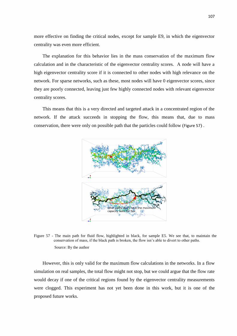
107
more effective on finding the critical nodes, except for sample E9, in which the eigenvector
centrality was even more efficient.
The explanation for this behavior lies in the mass conservation of the maximum flow
calculation and in the characteristic of the eigenvector centrality scores. A node will have a
high eigenvector centrality score if it is connected to other nodes with high relevance on the
network. For sparse networks, such as these, most nodes will have 0 eigenvector scores, since
they are poorly connected, leaving just few highly connected nodes with relevant eigenvector
centrality scores.
This means that this is a very directed and targeted attack in a concentrated region of the
network. If the attack succeeds in stopping the flow, this means that, due to mass
conservation, there were only on possible path that the particles could follow (Figure 57) .
Figure 57 - The main path for fluid flow, highlighted in black, for sample E5. We see that, to maintain the
conservation of mass, if the black path is broken, the flow isn’s able to divert to other paths.
Source: By the author
However, this is only valid for the maximum flow calculations in the networks. In a flow
simulation on real samples, the total flow might not stop, but we could argue that the flow rate
would decay if one of the critical regions found by the eigenvector centrality measurements
were clogged. This experiment has not yet been done in this work, but it is one of the
proposed future works.

109
6 CONCLUSIONS AND FUTURE WORK
We have proposed the use of network theory as a complementary tool to understand the
topology of porous materials. In our work, we developed a powerful method of network
extraction that could recover the morphological and topological features of our samples.
The medial axis networks proved to be efficient for the tortuosity measurement of the
samples. The modelling of the networks’ capacity was able to capture the paths with least
resistance for fluid flow, so the electrical tortuosity of the samples was recovered. This shows
that the topology of the final networks could describe correctly the features from the
volumetric data from the samples.
The test of the recovering of morphology of the samples was also successful. The pore
size distributions of the developed method corresponded to the pore size distribution captured
by commercial methods. However, the developed method has some advantages over the
commercial application:
(1) The pore space is divided according to the relevance of the pore centers inside the
complete network, this removes the necessity of adjustments made by the user of the
software;
(2) The regions identified as throats will always be regions with high connectivity in the
network, meaning that the throats will be the regions of preferential paths of fluid
flow.
The correspondence between the paths of flux observed in the direct simulations and the
paths found through maximum flow measurement in the networks showed that the final pore-
throat networks are also robust models for fluid flow, which, in turn, permitted that the
structure of the networks could be evaluated through network theory.
The evaluation through network theory showed that the pore-throat networks are not free-
scale, but follow an exponential decay on the connectivity of nodes. We were also able to
show that the closeness centrality distribution of the nodes provides important information on
the dynamics of fluid flow. Even though the local entropy of the nodes is low, meaning that
the variation between capacities of each throat connected to the pore is not very large, we still
find nodes with high closeness centrality on the sample with lowest absolute permeability

110
measured. This is an indication of the existence of nodes acting as bridges for the passage of
flux.
The nodes that were more important for flux was also determined through the robustness
test. Indeed, closeness centrality of a pore is correlated to the total flux of the sample. We
observed as well, that, for more homogeneous samples, there is little difference between
removing a pore with large volume from a more central one. However, for the heterogeneous
sample, removing a large pore is very crucial for fluid flow.
On the wormholes study, we could show that the method developed is an important
technique to evaluate the final structures after acidification. We could separate the influences
of the main channels of that of the ramifications. We were also able to show that, even though
the tortuosity of the sample is large, the ramification structure can play an important part on
the fluid extraction. Also, the robustness test was able to verify which sample channeling
structure could be more fragile to flaws.
We believe that this work is an important contribution to continue development of
methods and characterization of porous materials.
6.1 FUTURE WORK
For future work, we intend to use the development extraction method for the simulation
of dynamics of diffusion and NMR experiments inside the porous media.
We also intend to apply the method for more rock samples, carbonates and sandstones.
We see that complex network theory applied to porous medium is a powerful tool, so we
intend to apply for a large range of samples to make a statistical analysis of the porous space.
A first visualization of this application is shown on Figure 58, in which the sphere cell
network is used for the separation of the pore space into regions with long relaxation times
(larger radius) in contrast with regions with short relaxation times (smaller radius).
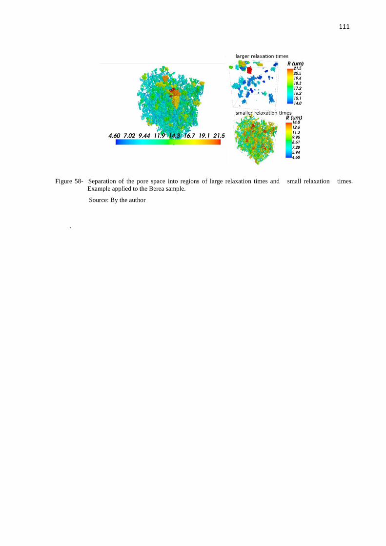
111
Figure 58- Separation of the pore space into regions of large relaxation times and small relaxation times.
Example applied to the Berea sample.
Source: By the author
.


113
REFERENCES
1 BERNABÉ, Y.; LI, M.; TANG, Y.-B.; EVANS, B. Pore space connectivity and the transport
properties of rocks. Oil & Gas Science and Technology – Revue d’IFP Energies nouvelles, v. 71, n. 4,
p. 50, 2016.
2 DEL COLLE, R.; FORTULAN, C. A.; FONTES, S. R. Manufacture and characterization of ultra
and microfiltration ceramic membranes by isostatic pressing. Ceramics International, v. 37, n. 4, p.
1161–1168, 2011.
3 CHAPPARD, C. et al. 3D characterization of pores in the cortical bone of human femur in the
elderly at different locations as determined by synchrotron micro-computed tomography images.
Osteoporosis International, v. 24, n. 3, p. 1023–1033, 2013.
4 PLECAS, I. B.; DIMOVIC, S. D. Mathematical modelling of transport phenomena in concrete
porous media. Materials Research Society Symposium Proceedings, v. 1193, p. 405–410, 2009.
5 FASHI, F. H. Review of solute transport modeling in soils and hydrodynamic dispersivity.
Conference: International Soil Science Congress 2015, v. 4, n. 3, p. 134–142, 2015.
6 VIEJO, I.; ESTEVES, L. P.; LASPALAS, M.; BIELSA, J. M. Numerical modelling of porous
cement-based materials by superabsorbent polymers. Cement and Concrete Research, v. 90, p. 184–
193, 2016.
7 SILVA, R. O. Utilização da RMN no estudo de rochas reservatório siliciclásticas. 2014. 207 p. Tese
(Doutorado em Ciências) - Instituto de Física de São Carlos, Universidade de São Paulo, São Carlos,
2014.
8 TSUCHIDA, J. E. et al. Characterization of fiber cement with inclusion of treated vegetable fibers
using NMR relaxometry. Brazilian Meeting on Magnetic Resonance, p. 140–141, 2012.
9 GIANNONI, R. A.; MONTRAZI, E. T.; CESAR, R.; BONAGAMBA, T. J. Application of nuclear
magnetic resonance in osteoporosis evaluation. Regional Congress of IRPA on security radiological
and nuclear security, v. 45, n. 2, p. 7, 2013.
10 MONTRAZI, E. T. Estudo de cerâmicas porosas de alumina através da medida de tempos de
relaxação via ressonância magnética nuclear. 2012. 164 p. Dissertação (Mestrado em Ciências) -
Instituto de Física de São Carlos, Universidade de São Paulo, São Carlos, 2012.
11 D’EURYDICE, M. N.; MONTRAZI, E. T.; FORTULAN, C. A.; BONAGAMBA, T. J. T 2-
Filtered T 2− T 2 Exchange NMR. Journal of Chemical Physics, v. 144, n. 20, p. 204201, 2016.
12 LUCAS-OLIVEIRA, É. Difusão de spins nucleares em meios porosos-uma abordagem
computacional da RMN. 2015. 141 p. Dissertação (Mestrado em Ciências) - Instituto de Física de São
Carlos, Universidade de São Paulo, São Carlos, 2015.
13 SAMEC, M. et al. Quantifying soil complexity using network models of soil porous structure.
Nonlinear Processes in Geophysics, v. 20, n. 1, p. 41–45, 2013.
14 VALENTINI, L.; PERUGINI, D.; POLI, G. The “small-world” topology of rock fracture networks.
Physica A: Statistical Mechanics and its Applications, v. 377, n. 1, p. 323–328, 2007.
15 BERKOWITZ, B. Characterizing flow and transport in fractured geological media: a review.
Advances in Water Resources, v. 25, n. 8–12, p. 861–884, 2002.
16 GHAFFARI, H. O.; SHARIFZADEH, M.; FALL, M. Analysis of aperture evolution in a rock joint
using a complex network approach. International Journal of Rock Mechanics and Mining Sciences, v.
47, n. 1, p. 17–29, 2010.

114
17 GHAFFARI, H. O.; SHARIFZADEH, M.; YOUNG, R. P. Complex aperture networks. Physica A:
statistical mechanics and its applications, v. 392, n. 4, p. 1028–1037, 2013.
18 SANDERSON, D. J.; NIXON, C. W. The use of topology in fracture network characterization.
Journal of Structural Geology, v. 72, n. 1, p. 55–66, 2015.
19 SANTIAGO, E.; VELASCO-HERNANDEZ, J. X.; ROMERO-SALCEDO, M. A descriptive study
of fracture networks in rocks using complex network metrics. Computers and Geosciences, v. 88, n. 1,
p. 97–114, 2016.
20 HORGAN, G.; MOLCHANOV, I.; SHCHERBAKOV, V.; ZUYEV, S. Approximate models for
bacteria leaching through porous media. Applied Mathematics and Computation, v. 188, n. 2, p. 1941–
1954, 2007.
21 BASSETT, D. S.; OWENS, E. T.; PORTER, M. A; MANNING, M. L.; DANIELS, K. E.
Extraction of force-chain network architecture in granular materials using community detection. Soft
Matter, v. 11, n. 14, p. 2731–44, 2015.
22 WALKER, D. M.; TORDESILLAS, A. Topological evolution in dense granular materials: A
complex networks perspective. International Journal of Solids and Structures, v. 47, n. 5, p. 624–639,
2010.
23 ALMHDIE, A.; ROZENBAUM, O.; LESPESSAILLES, E.; JENNANE, R. Image processing for
the non-destructive characterization of porous media. application to limestones and trabecular bones.
Mathematics and Computers in Simulation, v. 99, p. 82–94, 2014.
24 RICORDEAU, A.; MELLOULI, N. Exploring 3D-structure analysis tools for a simulated bone
remodelling process. Computer Methods in Biomechanics and Biomedical Engineering, v. 4, n. 1, p.
1–11, 2015.
25 JONES, A. C. et al. The correlation of pore morphology, interconnectivity and physical properties
of 3D ceramic scaffolds with bone ingrowth. Biomaterials, v. 30, n. 7, p. 1440–1451, 2009.
26 BALA, Y. et al. Pore network microarchitecture influences human cortical bone elasticity during
growth and aging. Journal of the Mechanical Behavior of Biomedical Materials, v. 63, n. 1, p. 164–
173, 2016.
27 VAN DER LINDEN, J. H.; NARSILIO, G. A.; TORDESILLAS, A. Machine learning framework
for analysis of transport through complex networks in porous, granular media: a focus on permeability.
Physical Review E, v. 94, n. 2, p. 1–16, 2016.
28 SILIN, D.; PATZEK, T. Pore space morphology analysis using maximal inscribed spheres. Physica
A: Statistical Mechanics and its Applications, v. 371, n. 2, p. 336–360, 2006.
29 BYHOLM, T.; TOIVAKKA, M.; WESTERHOLM, J. The application of morphological algorithms
on 3-dimensional porous structures for identifying pores and gathering statistical data. WSEAS
Transactions on Information Science and Applications, v. 3, n. 12, p. 2374–2380, 2006.
30 ARAND, F.; HESSER, J. Accurate and efficient maximal ball algorithm for pore network
extraction. Computers & Geosciences, v. 101, n. 1, p. 28–37, 2017.
31 AL-KHARUSI, A. S.; BLUNT, M. J. Network extraction from sandstone and carbonate pore space
images. Journal of Petroleum Science and Engineering, v. 56, n. 4, p. 219–231, 2007.
32 RABBANI, A.; JAMSHIDI, S.; SALEHI, S. An automated simple algorithm for realistic pore
network extraction from micro-tomography images. Journal of Petroleum Science and Engineering, v.
123, n. 1, p. 164–171, 2014.
33 AL-RAOUSH, R. I.; WILLSON, C. S. Extraction of physically realistic pore network properties
from three-dimensional synchrotron X-ray microtomography images of unconsolidated porous media
systems. Journal of Hydrology, v. 300, n. 1–4, p. 44–64, 2005.

115
34 XIONG, Q.; BAYCHEV, T. G.; JIVKOV, A. P. Review of pore network modelling of porous
media: Experimental characterisations, network constructions and applications to reactive transport.
Journal of Contaminant Hydrology, v. 192, p. 101–117, 2016.
35 AL-RAOUSH, R.; THOMPSON, K.; WILLSON, C. S. Comparison of network generation
techniques for unconsolidated porous media. Soil Science Society of America Journal, v. 67, n. 6, p.
1687, 2003.
36 BAKKE, S.; ØREN, P.-E.; A. 3-D pore-scale modelling of sandstones and flow simulations in the
pore networks. Society of Petroleum Engineers, v. 2, n. 1, p. 136--149, 1997.
37 BLUNT, M. J. et al. Pore-scale imaging and modelling. Advances in Water Resources, v. 51, p.
197–216, 2013.
38 SILIN, D. B.; JIN, G. D.; PATZEK, T. W. Robust determination of the pore-space morphology in
sedimentary rocks. Journal of Petroleum Geology, v. 56, n. 5, p. 69–70, 2004.
39 TALABI, O.; ALSAYARI, S.; IGLAUER, S.; J. BLUNT, M.; BLUNT, M. J. Pore-scale simulation
of NMR response. Journal of Petroleum Science and Engineering, v. 67, n. 3–4, p. 168–178, 2009.
40 KREBS, M. et al. The first visualization of acid treatments on carbonates with 3D nuclear magnetic
resonance imaging (NMRI). SPE Journal, v. 20, n. 4, p. 26–28, 2015.
41 MCDUFF, D.; JACKSON, S.; SHUCHART, C.; POSTL, D. Understanding wormholes in
carbonates. Journal of Petroleum Technology, v. 62, n. 10, p. 78–81, 2010.
42 BARABÁSI, A. L. The physics of the Web. Physics World, v. 14, n. 7, p. 33–38, 2001.
43 BARRAT, A.; BARTHÉLEMY, M.; VESPIGNANI, A. Dynamical processes on complex
networks. Cambridge: Cambridge University Press, 2008.
44 NEWMAN, M. Networks: An Introduction. New York: Oxford University Press, 2010.
45 TAINA, I. A; HECK, R. J.; ELLIOT, T. R. Application of X-ray computed tomography to soil
science: a literature review. Canadian Journal of Soil Science, v. 88, n. 1, p. 1–19, 2008.
46 LIU, J.; PEREIRA, G. G.; LIU, Q.; REGENAUER-LIEB, K. Computational challenges in the
analyses of petrophysics using microtomography and upscaling: a review. Computers and
Geosciences, v. 89, p. 107–117, 2016.
47 MEES, F.; SWENNEN, R.; VAN GEET, M.; JACOBS, P. Applications of X-ray computed
tomography in the geosciences. Geological Society, Special Publications, v. 215, n. 1, p. 1–6, 2003.
48 CNUDDE, V.; BOONE, M. N. High-resolution X-ray computed tomography in geosciences: a
review of the current technology and applications. Earth-Science Reviews, v. 123, p. 1–17, 2013.
49 COLGATE, S. A. Gamma-Ray Absorption Measurements. Physical Review B, v. 87, n. 4, p. 592–
601, 1952.
50 PERGEOS for digital rock and core analysis. Disponível em:
<https://www.fei.com/software/pergeos-for-oil-gas/>. Acesso em: 20 jan. 2017.
51 BLUNT, M. J. Multiphase flow in permeable media: a pore-scale perspective. Cambridge:
Cambridge University Press, 2016.
52 BERG, C. F.; HELD, R. Fundamental transport property relations in porous media incorporating
detailed pore structure description. Transport in Porous Media, v. 112, n. 2, p. 467–487, 2016.
53 ARCHIE, G. E. The electrical resistivity log as an aid in determining some reservoir
characteristics. Petroleum Technology, v. 4, n. 1, p. 54–62, 1942.

116
54 CINAR, Y. et al. Formation factor for heterogeneous carbonate rocks using multi-scale X-ray CT
images. SPE KUWAIT INTERNATIONAL PETROLEUM CONFERENCE AND EXHIBITION,
2012, Kuwait City. Proceedings… Kuwait City: Society of Petroleum Engineers, 2012.
55 TUMIDAJSKI, P. J. et al. A model for calculating the formation resistivity factor in low and
middle porosity sandstone formations considering the effect of pore geometry. Journal of Petroleum
Science and Engineering, v. 77, n. 2, p. 185–206, 2017.
56 SUMAN, R.; RUTH, D. Formation factor and tortuosity of homogeneous porous media. Transport
in Porous Media, v. 12, n. 2, p. 185–206, 1993.
57 TUMIDAJSKI, P. J.; SCHUMACHER, A. S.; PERRON, S.; GU, P.; BEAUDOIN, J. J. On the
relationship between porosity and electrical resistivity in cementitious systems. Cement and Concrete
Research, v. 26, n. 4, p. 539–544, 1996.
58 KATSUBE, T. J. Review of formation resistivity factor equations related to new pore-structure
concepts. Current Research, v. 7, p. 9, 2010.
59 BELTRÁN, A. et al. A new model for the computation of the formation factor of core rocks.
Journal of Structural Geology, v. 97, p. 189–198, 2017.
60 GARROUCH, A. A.; ALI, L.; QASEM, F. Using diffusion and electrical measurements to assess
tortuosity of porous media. Industrial & Engineering Chemistry Research, v. 40, n. 20, p. 4363–4369,
2001.
61 BERNABÉ, Y.; ZAMORA, M.; LI, M.; MAINEULT, A.; TANG, Y. B. Pore connectivity,
permeability, and electrical formation factor: a new model and comparison to experimental data.
Journal of Geophysical Research: Solid Earth, v. 116, n. 11, p. 1–15, 2011.
62 GHANBARIAN, B.; HUNT, A. G.; EWING, R. P.; SAHIMI, M. Tortuosity in porous Media. Soil
Science Society of America Journal, v. 77, n. 5, p. 1461–1477, 2013.
63 AZAR, J. H.; JAVAHERIAN, A.; PISHVAIE, M. R.; NABI-BIDHENDI, M. An approach to
defining tortuosity and cementation factor in carbonate reservoir rocks. Journal of Petroleum Science
and Engineering, v. 60, n. 2, p. 125–131, 2008.
64 KÄRGER, J.; VALIULLIN, R. Diffusion theory for transport in porous media. Encyclopedia of
Magnetic Resonance, v. 34, n. 7, p. 1685–1693, 1998.
65 CHURCHER, P. L. Rock properties of Berea sandstone, Baker dolomite, and Indiana limestone.
SPE International Symposium on Oilfield Chemistry, v. 21, n. 44, p. 431–466, 1991.
66 SHARQAWY, M. H. Construction of pore network models for Berea and Fontainebleau
sandstones using non-linear programing and optimization techniques. Advances in Water Resources, v.
98, p. 198–210, 2016.
67 GHARBI, O. et al. Carbon storage fundamentals - changes in pore structure and connectivity
induced by CO₂ injection in carbonates: a combined pore-scale approach. COP18-Collection, v. 2012,
COP18, EEPS21. doi: 10.5339/qfarf.2012.
68 OTT, H.; PENTLAND, C. H.; OEDAI, S. CO2-brine displacement in heterogeneous carbonates.
International Journal of Greenhouse Gas Control, v. 33, p. 135–144, 2015.
69 VIALLE, S. et al. Percolation of CO2-rich fluids in a limestone sample: Evolution of hydraulic,
electrical, chemical, and structural properties. Journal of Geophysical Research: solid earth, v. 119, n.
4, p. 2828–2847, 2014.
70 Digital rocks portal. Disponível em: <https://www.digitalrocksportal.org/projects/10/sample/7/>.
Acesso em: 20 jan. 2017.
71 KALFAYAN, L. Production enhancement with acid stimulation. PennWell, 2000.
117
72 BYHOLM, T.; ALAM, P.; WESTERHOLM, J.; TOIVAKKA, M. The use of morphological
algorithms and finite difference methods on 3-dimensional paper coating structures for identifying
pores , gathering statistical data and physical constants. 6th WSEAS International Conference on
Simulation, Modelling and Optimization, p. 264–270, 2006.
73 STOECKEL, D. et al. Morphological analysis of disordered macroporous-mesoporous solids based
on physical reconstruction by nanoscale tomography. Langmuir, v. 30, n. 30, p. 9022–9027, 2014.
74 MENDOZA, F. et al. Three-dimensional pore space quantification of apple tissue using X-ray
computed microtomography. Planta, v. 226, n. 3, p. 559–570, 2007.
75 HORMANN, K.; BARANAU, V.; HLUSHKOU, D.; HOLTZEL, A.; TALLAREK, U. Topological
analysis of non-granular{,} disordered porous media: determination of pore connectivity{,} pore
coordination{,} and geometric tortuosity in physically reconstructed silica monoliths. New J. Chem.,
2016.
76 YANG, F. et al. Extraction of pore-morphology and capillary pressure curves of porous media from
synchrotron-based tomography data. Scientific Reports, v. 5, n. April, p. 10635, 2015.
77 SHEPPARD, A. P.; SOK, R. M.; AVERDUNK, H. Improved pore network extraction methods.
International Symposium of the Society of Core Analysts, v. 2, n. 3, p. 1–11, 2005.
78 ROERDINK, J.; MEIJSTER, A. The watershed transform: definitions, algorithms and
parallelization strategies. Fundamenta Informaticae, v. 41, n. 1–2, p. 187–228, 2000.
79 VIDELA, A.; LIN, C.-L.; MILLER, J. D. Watershed functions applied to a 3D image segmentation
problem for the analysis of packed particle beds. Particle & Particle Systems Characterization, v. 23,
n. 3–4, p. 237–245, 2006.
80 DONG, H.; BLUNT, M. J. Pore-network extraction from micro-computerized-tomography images.
Physical Review E - Statistical, Nonlinear, and Soft Matter Physics, v. 80, n. 3, p. 1–11, 2009.
81 GOODRICH, M. T.; TAMASSIA, R.; GOLDWASSER, M. H. Data structures and algorithms in
python. Hoboken: John Wiley & Sons, 2013.
82 CLAUDINE, D. Combined use of x-ray CT scan and local resistivity measurements: a new
approach to fluid distribution description in cores. In: SPE ANNUAL TECHNICAL CONFERENCE
AND EXHIBITION, 2003, Denver. Proceedings… Denver: Society of Petroleum Engineers, 2003.
83 HAN, M. et al. The effect of the porous structure on resistivity index curves. an experimental and
numerical study. In: ANNUAL LOGGING SYMPOSIUM, 49., 2008, Austin. Proceedings… Austin:
Society of Petrophysicists and Well-Log Analysts, 2008.
84 MOSTAGHIMI, P.; LIU, M.; ARNS, C. H. Numerical simulation of reactive transport on micro-ct
images. Mathematical Geosciences, v. 48, n. 8, p. 963–983, 2016.
85 VASILYEV, L.; RAOOF, A.; NORDBOTTEN, J. M. Effect of mean network coordination number
on dispersivity characteristics. Transport in Porous Media, v. 95, n. 2, p. 447–463, 2012.
86 FAUZI, U. Influence of coordination number and percolation probability on rock permeability
estimation. Geophysical Research Letters, v. 29, n. 8, p. 8–11, 2002.
87 CLAUSET, A. et al. Power-Law Distributions in Empirical Data. SIAM Review, v. 51, n. 4, p. 661–
703, 2009.
88 DENG, W.; LI, W.; CAI, X.; WANG, Q. A. The exponential degree distribution in complex
networks: Non-equilibrium network theory, numerical simulation and empirical data. Physica A:
statistical mechanics and its applications, v. 390, n. 8, p. 1481–1485, 2011.
89 ALBERT, R.; BARABASI, A. L. Statistical mechanics of complex networks. Reviews of Modern
Physics, v. 74, n. 1, p. 47–97, 2002.