Topology and geometry optimization of elastic structures byexact deformation of simplicial mesh

Gregoire Allaire a,1, Charles Dapogny b,c , Pascal Frey c

aCentre de Mathematiques Appliquees (UMR 7641), Ecole Polytechnique 91128 Palaiseau, FrancebRenault DREAM-DELT’A Guyancourt, France

cUPMC Univ Paris 06, UMR 7598, Laboratoire J.-L. Lions, F-75005, Paris, France

Received *****; accepted after revision +++++

Presented by

Abstract

We propose a method for structural optimization that relies on two alternative descriptions of shapes : on the onehand, they are exactly meshed so that mechanical evaluations by finite elements are accurate ; on the other hand,we resort to a level-set characterization to describe their deformation along the shape gradient. The key ingredientis a meshing algorithm for building a mesh, suitable for numerical computations, out of a piecewise linear level-setfunction on an unstructured mesh. Therefore, our approach is at the same time a geometric optimization method(since shapes are exactly meshed) and a topology optimization method (since the topology of successive shapescan change thanks to the power of the level-set method). To cite this article: G. Allaire, C. Dapogny, P. Frey, C.R. Acad. Sci. Paris, Ser. I 340 (2005).

Resume

Optimisation topologique et geometrique de structures elastiques par deformation exacte de maillagesimplicial On presente dans cette note une methode d’optimisation structurale qui s’appuie sur deux manierescomplementaires de representer des formes : d’une part, elles sont maillees exactement afin que l’evaluation desperformances mecaniques par elements finis soit precise ; d’autre part, on utilise leur representation a l’aide d’unefonction de lignes de niveaux pour les deformer suivant le gradient de forme. L’ingredient crucial est un algorithmede remaillage qui permet de construire un maillage, de qualite appropriee pour les calculs numeriques, a partird’une fonction ligne de niveaux continue et affine par morceaux sur un maillage non structure. Par consequent,notre approche peut etre vue a la fois comme une methode d’optimisation geometrique (puisque les structuressont maillees exactement) et comme une methode d’optimisation topologique (puisque la topologie des formessuccessives peut changer grace a l’utilisation de l’algorithme des lignes de niveaux). Pour citer cet article : G.Allaire, C. Dapogny, P. Frey, C. R. Acad. Sci. Paris, Ser. I 340 (2005).

Email addresses: gregoire.allaire@polytechnique.fr (Gregoire Allaire), dapogny@ann.jussieu.fr (CharlesDapogny), frey@ann.jussieu.fr (Pascal Frey).

1 . G. A. is a member of the DEFI project at INRIA Saclay Ile-de-France and is partially supported by the Chair

Preprint submitted to the Academie des sciences 30 novembre 2011

Version francaise abregee

Classiquement, l’optimisation structurale repose sur la methode de Hadamard [1], [12], [17] qui prescritla deformation de la frontiere d’un domaine Ω (donnant lieu a une suite de formes Ωk) pour que celui-ciminimise une certaine fonction-objectif. D’un point de vue technique, ceci se traduit par la necessitede deformer le maillage de la forme courante (maillage qui permet d’effectuer des calculs par elementsfinis), ce qui s’avere tres difficile, voire impossible, notamment en trois dimensions. Pour remedier a cetinconvenient majeur, de recents developpements [2], [3], [19] ont conduit a regarder le probleme sous l’anglede la methode des lignes de niveaux de Osher et Sethian [13]. Le bord du domaine est represente commeligne de niveau 0 d’une fonction implicite definie sur un domaine de calcul fixe D (maille typiquementpar une grille cartesienne) dont l’evolution est regie par une equation de type Hamilton-Jacobi. Celanecessite de pouvoir donner un sens au probleme mecanique considere sur tout le domaine de calcul etpas seulement dans la forme Ωk, ce qui dans le contexte de l’elasticite se fait en considerant que le milieuexterieur D \ Ωk n’est pas vide mais occupe par un materiau “ersatz” tres mou.

Dans cette note, on propose une nouvelle approche au confluent de ces deux cadres de travail : d’unepart, comme dans l’approche classique, on continue a mailler exactement chaque forme Ωk a l’iteration kde l’algorithme d’optimisation ; d’autre part, l’evolution de la forme d’une iteration a l’autre est toujoursdecrite par la methode des lignes de niveaux, mais sur un maillage non structure (simplicial) du domaine decalcul D, que l’on s’autorise a modifier d’une iteration a l’autre. Puisque les maillages sont non structuresla methode des lignes de niveaux ne peut utiliser des schemas usuels de type difference finies : ici, onutilise une methode des caracteristiques [14], [18]. Il n’y a ensuite plus qu’a garder la partie interieure a laforme de ce maillage pour proceder a l’evaluation de sa performance mecanique par un calcul d’elementsfinis. Il est ainsi possible de decrire des changements importants (y compris des changements de topologie)de la forme alors que celle-ci reste maillee exactement a chaque etape. La methode est presentee ici surdes exemples en 2d (voir les figures 1 et 2), mais a l’avantage de ne pas presenter d’obstacle conceptuel aune extension en 3d, contrairement a beaucoup d’heuristiques quant a l’evolution du maillage.

1. Introduction

Since [2], [3] and [19], the level-set method of Osher and Sethian [13] has proved to be a very versatiletool in the context of structural optimization. Working on a fixed Cartesian grid of a large computationaldomain D ⊂ Rd, the authors used a consistant approximation of the mechanical problem at stake -namely the ersatz material approach - then applied classical shape sensitivity techniques (the so-calledHadamard method [1], [12], [17]) and described the evolution of the shape Ω ⊂ D by a Hamilton-Jacobiequation for the associated level-set function. In this note, we propose a new approach where the shapeΩ is exactly meshed and no ersatz material is necessary in the void region D \Ω. We still rely on a largercomputational domain D which is no longer meshed with a fixed Cartesian grid, but rather is endowedwith an unstructured mesh that is notably changed at each iteration of the optimization process (usinglocal mesh modification techniques [9]) so that the shape Ω is precisely captured, i.e. its boundary isa collection of internal edges (in 2d) or faces (in 3d) of the mesh. The level-set method is still a keyingredient for mesh deformation and, as such, allows for topology changes from one iteration to the next.However, we are inherently working on unstructured meshes, hence we cannot rely on finite differenceschemes and we rather use a method of characteristics [14], [18]. We emphasize that, even though all our

”Mathematical modelling and numerical simulation, F-EADS - Ecole Polytechnique - INRIA”.

2

numerical examples here are in the 2d setting, the whole method has been devised so that there is noadditional conceptual difficulty for the 3d case, especially as regards the strategy for mesh evolution.

2. Description of the problem and notations

As a model problem, we are interested in the optimization of a shape Ω, that is, a bounded domain ofRd, made of a linear isotropic material, with Hooke’s law A. Such a shape is clamped on a part ΓD of itsboundary ∂Ω, and submitted to surface loads g ∈ H2(Rd)d on the complementary part ΓN = ∂Ω \ ΓD

(with ΓD and ΓN being of positive (d − 1)-measure in ∂Ω). For the sake of simplicity, we neglect bodyforces and restrict ourselves to linearized elasticity. In this context, the displacement field u = uΩ of theshape is the unique solution in H1(Ω)d of the elasticity system −div(Ae(u)) = 0 in Ω,

u = 0 on ΓD, Ae(u) · n = g on ΓN ,(1)

where e(u) = 12 ((∇u)t +∇u) is the strain tensor and n is the outer unit normal to ∂Ω. We aim at finding

a shape Ω that minimizes a given objective function J(Ω) in a set Uad of admissible shapes which mayinvolve geometric constraints such as Ω ⊂ D and a fixed total volume V (Ω). In this note, we restrictourselves to the compliance (which is a global measure of the rigidity of the structure Ω) and the volumeconstraint is taken into account through a Lagrangian with a fixed positive Lagrange multiplier `, so thatthe optimization problem becomes

infΩ⊂D

(J(Ω) + ` V (Ω)

)with J(Ω) =

∫ΓN

g · uΩ ds. (2)

As explained in [3], there are no difficulties to extend our approach to more general objective functions,to additional constraints and to non-linear elasticity.

3. Two complementary ways for representing shapes

We alternatively represent a shape Ω ⊂ D as a mesh TΩ of the whole computational domain D in whichΩ is explicitly discretized (so that a mesh of Ω is included in TΩ as a submesh - see figure 2) and as alevel-set function ψΩ, defined on D (in numerical practice it is a P1-Lagrange finite element function onan unstructured mesh), enjoying the properties

Ω = x ∈ D \ ψΩ(x) < 0 ; ∂Ω = x ∈ D \ ψΩ(x) = 0 . (3)

Both representations are used at different steps of our method: thus, a crucial ingredient is an efficientalgorithm for passing from one characterization to the other.Generating a level-set function associated to a shape. Let Ω ⊂ D be a subdomain, explicitlydiscretized in the mesh T of D (even though the method straightforwardly extends to the case of anon-discretized interface). It is classical to generate a corresponding level-set function by computing thesigned distance function to Ω, at least near the interface ∂Ω [6]. To this end, we use a numerical schemefor unstructured (simplicial) meshes, based on some properties of the unique viscosity solution of thetime-dependent Eikonal equation, which is described in detail in a previous work [7] (see e.g. [15] for analternative).Meshing the negative subdomain of a level set function, ensuring conformity with the posi-tive subdomain. Given an initial triangular mesh T of D, the 0 level-set of a P1 finite element function

3

ψ is a piecewise affine curve (surface in 3d). To obtain a (new) mesh of the shape Ω, corresponding to ψthrough (3), we proceed in two (or three) steps :

(i) Each simplex K ∈ T , crossed by the 0 level-set of function ψ is cut in such a way that K ∩ ∂Ω

belongs to the resulting mesh T , which has to remain conformal. To this end, a pattern whichenumerates the various possible configurations is used [9]. Unfortunately, the intersections of ∂Ω

with the mesh T are not controlled and the obtained mesh T is bound to be of very poor qualityas far as finite element computations are concerned (ill-shaped elements, e.g. very flat or small, arelikely to appear).

(ii) A local mesh improvement is performed, so that a new improved quality mesh T ′ is created. Thisstep relies on local mesh modification operators (collapse of close points, points relocations,...)described in [9].

(iii) (Optional) The mesh T ′ is smoothed, especially near the boundary ∂Ω, with a mesh regularizationprocedure [9] to remove small angles or bumps on ∂Ω that could impair the accuracy of the finiteelement computations to come.

4. Shape and topological sensitivity analysis

Shape sensitivity analysis. This is the so-called Hadamard method [1], [12], [17] which has alreadybeen implemented in the context of level-set methods [2], [3]. Given a reference bounded domain Ω0, forθ ∈W 1,∞(Rd,Rd) small enough, (I+θ) is a Lipschitz diffeomorphism of Rd, with Lipschitz inverse and weconsider variations of the form Θad 3 θ 7→ (I + θ)Ω0 ∈ Rd, where Θad is a subset of W 1,∞(Rd,Rd) corre-sponding to admissible variations of the shape. An objective function J(Ω) is called shape-differentiable atΩ0 if the application θ 7→ J((I+θ)Ω0) is Frechet-differentiable at 0 and the associated Frechet differentialJ ′(Ω0)(θ) is the shape derivative of J at Ω0.

Let Ω ⊂ Rd be a smooth domain, it is well-known [3] that the compliance J(Ω) is shape-differentiableat Ω. Denoting by κ the mean curvature of ∂Ω, for any θ ∈ Θad, its shape derivative reads

J ′(Ω)(θ) =

∫ΓN

(2

(∂(g · uΩ)

∂n+ κg · uΩ

)−Ae(uΩ) : e(uΩ)

)θ · n ds+

∫ΓD

Ae(uΩ) : e(uΩ) θ · n ds. (4)

This yields a continuous velocity field θ (which is then to be numerically discretized in the finite elementsframework), equal to minus the scalar integrand multiplied by the normal n, a priori defined on theboundary ∂Ω, according to which this boundary has to be deformed so as to decrease the objectivefunction under consideration. Note that because this deformation is accounted for by level set methodsin our context, this velocity field has to be extended to the whole computational domain, following aregularization process described in [5], [11].Topological sensitivity analysis. The previous method produces a deformation of the boundary ∂Ωthat allows us to decrease the value of J(Ω), but forbids the creation of new holes in the domain: theresulting shape is thus strongly dependent on the initialization of the algorithm. As proposed in [4]it should be coupled with the so-called topological gradient [8], [10], [17] which is a mechanism thatevaluates the benefit of the formation of a small hole. This coupled strategy has the effect of making theoptimization process less dependent on the initialization (especially in 2d). Its implementation is similarto that in [4]: every 5 or 10 iterations of the optimization process, we compute the topological gradientand select the 2 or 3% most negative locations where we change the sign of the level-set function, thuscreating holes in the current shape. After discretizing on the mesh of D the resulting 0-level set of thismodified function, we start again the geometric optimization process.

4

5. Numerical algorithm

Starting from an initial shape Ω0 (e.g. the full computational domain D), we get a decreasing sequenceΩk of shapes with respect to function J by applying a shape-sensitivity analysis (section 4) on the actualdomain discretized under the form of a computational mesh, and evolve it with respect to the obtainedshape derivative resorting to a level-set description. From times to times (say, every ktop step), we performa topological sensitivity analysis instead of a shape sensitivity analysis so as to change the topology ofthe shape if need be. The proposed steepest-descent algorithm reads as follows (for clarity, we reportedonly the steps related to shape-sensitivity analysis, the other ones being easier) :

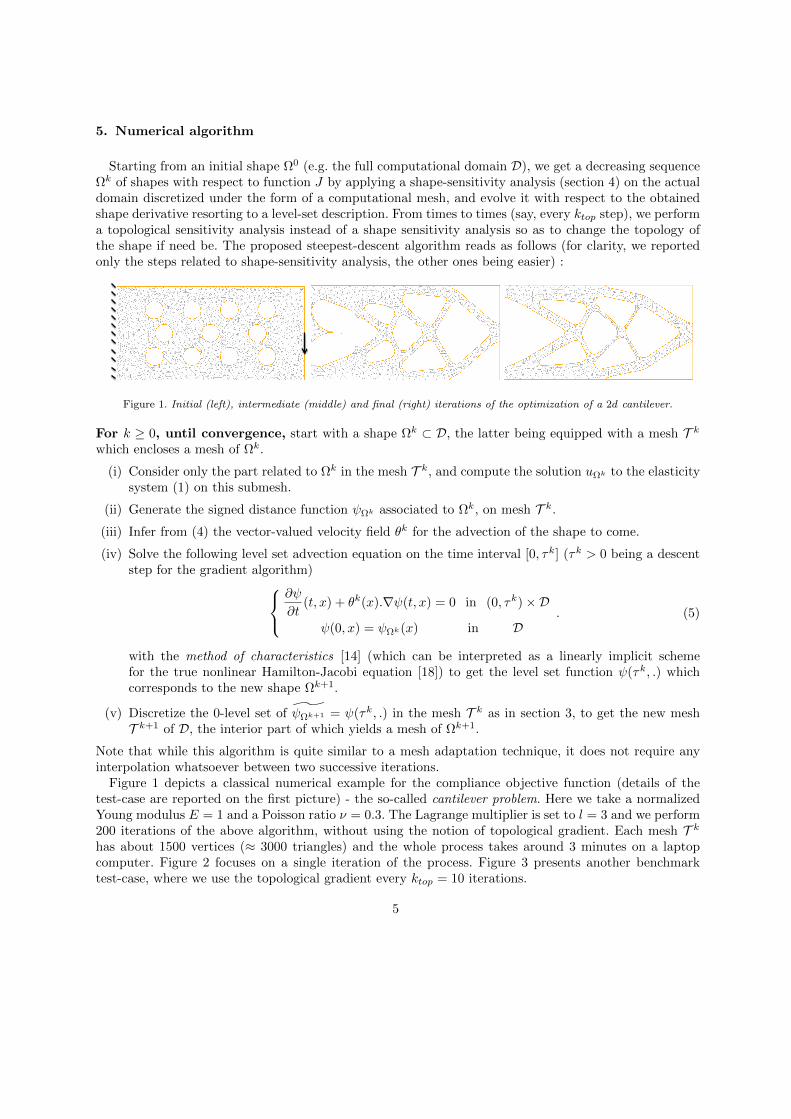
Figure 1. Initial (left), intermediate (middle) and final (right) iterations of the optimization of a 2d cantilever.

For k ≥ 0, until convergence, start with a shape Ωk ⊂ D, the latter being equipped with a mesh T k

which encloses a mesh of Ωk.

(i) Consider only the part related to Ωk in the mesh T k, and compute the solution uΩk to the elasticitysystem (1) on this submesh.

(ii) Generate the signed distance function ψΩk associated to Ωk, on mesh T k.

(iii) Infer from (4) the vector-valued velocity field θk for the advection of the shape to come.

(iv) Solve the following level set advection equation on the time interval [0, τk] (τk > 0 being a descentstep for the gradient algorithm)

∂ψ

∂t(t, x) + θk(x).∇ψ(t, x) = 0 in (0, τk)×D

ψ(0, x) = ψΩk(x) in D. (5)

with the method of characteristics [14] (which can be interpreted as a linearly implicit schemefor the true nonlinear Hamilton-Jacobi equation [18]) to get the level set function ψ(τk, .) whichcorresponds to the new shape Ωk+1.

(v) Discretize the 0-level set of ψΩk+1 = ψ(τk, .) in the mesh T k as in section 3, to get the new meshT k+1 of D, the interior part of which yields a mesh of Ωk+1.

Note that while this algorithm is quite similar to a mesh adaptation technique, it does not require anyinterpolation whatsoever between two successive iterations.

Figure 1 depicts a classical numerical example for the compliance objective function (details of thetest-case are reported on the first picture) - the so-called cantilever problem. Here we take a normalizedYoung modulus E = 1 and a Poisson ratio ν = 0.3. The Lagrange multiplier is set to l = 3 and we perform200 iterations of the above algorithm, without using the notion of topological gradient. Each mesh T k

has about 1500 vertices (≈ 3000 triangles) and the whole process takes around 3 minutes on a laptopcomputer. Figure 2 focuses on a single iteration of the process. Figure 3 presents another benchmarktest-case, where we use the topological gradient every ktop = 10 iterations.

5

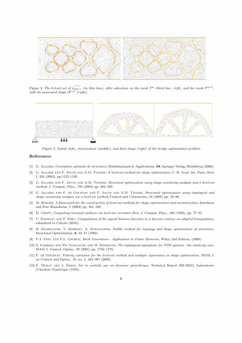
Figure 2. The 0-level set of ψΩk+1 (in thin line), after advection on the mesh T k (thick line ; left), and the mesh T k+1,

with its associated shape Ωk+1 (right).

Figure 3. Initial (left), intermediate (middle), and final shape (right) of the bridge optimization problem.

References

[1] G. Allaire, Conception optimale de structures, Mathematiques & Applications, 58, Springer Verlag, Heidelberg (2006).

[2] G. Allaire and F. Jouve and A.M. Toader, A level-set method for shape optimization, C. R. Acad. Sci. Paris, Serie

I, 334 (2002), pp.1125-1130.

[3] G. Allaire and F. Jouve and A.M. Toader, Structural optimization using shape sensitivity analysis and a level-setmethod, J. Comput. Phys., 194 (2004) pp. 363–393.

[4] G. Allaire and F. de Gournay and F. Jouve and A.M. Toader, Structural optimization using topological andshape sensitivity analysis via a level-set method, Control and Cybernetics, 34 (2005) pp. 59–80.

[5] M. Burger, A framework for the construction of level-set methods for shape optimization and reconstruction, Interfacesand Free Boundaries, 5 (2003) pp. 301–329.

[6] D. Chopp, Computing minimal surfaces via level-set curvature flow, J. Comput. Phys., 106 (1993), pp. 77–91.

[7] C. Dapogny and P. Frey, Computation of the signed distance function to a discrete contour on adapted triangulation,submitted to Calcolo (2010).

[8] H. Eschenauer, V. Kobelev, A. Schumacher, Bubble method for topology and shape optimization of structures,Structural Optimization, 8, 42–51 (1994).

[9] P.J. Frey and P.L. George, Mesh Generation : Application to Finite Elements, Wiley, 2nd Edition, (2008).

[10] S. Garreau and Ph. Guillaume and M. Masmoudi, The topological asymptotic for PDE systems : the elasticity case,

SIAM J. Control. Optim., 39 (2001) pp. 1756–1778.

[11] F. de Gournay, Velocity extension for the level-set method and multiple eigenvalues in shape optimization. SIAM J.

on Control and Optim., 45, no. 1, 343–367 (2006).

[12] F. Murat and J. Simon, Sur le controle par un domaine geometrique, Technical Report RR-76015, Laboratoired’Analyse Numerique (1976).

6

[13] S.J. Osher and J.A. Sethian, Fronts propagating with curvature-dependent speed : Algorithms based on Hamilton-

Jacobi formulations, J. Comput. Phys., 79 (1988), pp. 12–49.

[14] O. Pironneau, The finite element methods for fluids., Wiley (1989).

[15] R. Kimmel and J.A. Sethian, Computing Geodesic Paths on Manifolds, Proc. Nat. Acad. Sci. , 95 (1998), pp. 8431–

8435.

[16] J. Soko lowski, A. Zochowski, Topological derivatives of shape functionals for elasticity systems. Mech. StructuresMach., 29, no. 3, 331–349 (2001).

[17] J. Sokolowski and J.-P. Zolesio, Introduction to Shape Optimization : Shape Sensitivity Analysis, Springer Ser.

Comput. Math., vol. 10, Springer, Berlin (1992).

[18] J. Strain, Semi-Lagrangian Methods for Level Set Equations, J. Comput. Phys., 151 (1999) pp. 498–533.

[19] M.Y. Wang, X. Wang, D. Guo, A level set method for structural topology optimization, Comput. Methods Appl.

Mech. Engrg., 192, 227–246 (2003).

7