IEEE TRANSACTIONS ON CONTROL OF NETWORK SYSTEMS, VOL. 5, NO. 3, SEPTEMBER 2018 1075

Topology Design for Stochastically ForcedConsensus Networks

Sepideh Hassan-Moghaddam, Student Member, IEEE, and Mihailo R. Jovanovic , Senior Member, IEEE

Abstract—We study an optimal control problem aimed at addinga certain number of edges to an undirected network, with a knowngraph Laplacian, in order to optimally enhance closed-loop perfor-mance. The performance is quantified by the steady-state varianceamplification of the network with additive stochastic disturbances.To promote controller sparsity, we introduce �1 -regularization intothe optimal H2 formulation and cast the design problem as asemidefinite program. We derive a Lagrange dual, provide inter-pretation of dual variables, and exploit structure of the optimalityconditions for undirected networks to develop customized proxi-mal gradient and Newton algorithms that are well suited for largeproblems. We illustrate that our algorithms can solve the prob-lems with more than million edges in the controller graph in a fewminutes, on a PC. We also exploit structure of connected resistivenetworks to demonstrate how additional edges can be systemati-cally added in order to minimize the H2 norm of the closed-loopsystem.

Index Terms—Convex optimization, coordinate descent, ef-fective resistance, �1 -regularization, network coherence, proxi-mal gradient and Newton methods, semidefinite programming,sparsity-promoting control, stochastically forced networks.

I. INTRODUCTION

CONVENTIONAL optimal control of distributed systemsrelies on centralized implementation of control policies.

In large networks of dynamical systems, centralized informationprocessing imposes a heavy burden on individual nodes and isoften infeasible. This motivates the development of distributedcontrol strategies that require limited information exchange be-tween the nodes to reach consensus or guarantee synchroniza-tion. Over the last decade, a vast body of literature has dealtwith analysis, fundamental performance limitations, and designof distributed averaging protocols; e.g., see [1]–[8].

Optimal design of the edge weights for networks with pre-specified topology has received significant attention. In [2], thedesign of the fastest averaging protocol for undirected networkswas cast as a semidefinite program (SDP). Two customizedalgorithms, based on primal barrier interior-point (IP) and

Manuscript received October 17, 2016; revised January 27, 2017; acceptedFebruary 20, 2017. Date of publication February 24, 2017; date of current ver-sion September 17, 2018. This work was supported in part by the 3M GraduateFellowship, in part by the UMN Informatics Institute Transdisciplinary Fac-ulty Fellowship, and in part by the National Science Foundation under awardECCS-1407958. Recommended by Associate Editor S. Martinez

The authors are with the Ming Hsieh Department of Electrical Engineer-ing, University of Southern California, Los Angeles, CA 90089 USA (e-mail:,hassanmo@usc.edu; mihailo@usc.edu).

Digital Object Identifier 10.1109/TCNS.2017.2674962

subgradient methods, were developed and the advantages ofoptimal weight selection over commonly used heuristics weredemonstrated. Similar SDP characterization, for networks withstate-dependent graph Laplacians, was provided in [3]. The al-location of symmetric edge weights that minimize the mean-square deviation from average for networks with additivestochastic disturbances was solved in [4]. A related problem,aimed at minimizing the total effective resistance of resistivenetworks, was addressed in [6]. In [7], the edge Laplacian wasused to provide graph-theoretic characterization of the H2 andH∞ symmetric agreement protocols.

Network coherence quantifies the ability of distributed esti-mation and control strategies to guard against exogenous dis-turbances [5], [8]. The coherence is determined by the sumof reciprocals of the nonzero eigenvalues of the graph Lapla-cian and its scaling properties cannot be predicted by alge-braic connectivity of the network. In [8], performance limi-tations of spatially localized consensus protocols on regularlattices were examined. It was shown that the fundamentallimitations for large-scale networks are dictated by the net-work topology rather than by the optimal selection of the edgeweights. Moreover, epidemic spread in networks is strongly in-fluenced by their topology [9]–[11]. Thus, optimal topology de-sign represents an important challenge. It is precisely this prob-lem, for undirected consensus networks, that we address in thepaper.

More specifically, we study an optimal control problem aimedat achieving a desired tradeoff between the network perfor-mance and communication requirements in the distributed con-troller. Our goal is to add a certain number of edges to a givenundirected network in order to optimally enhance the closed-loop performance. One of our key contributions is the formu-lation of topology design as an optimal control problem thatadmits convex characterization and is amenable to the develop-ment of efficient optimization algorithms. In our formulation,the plant network can contain disconnected components andoptimal topology of the controller network is an integral partof the design. In general, this problem is NP-hard [12] and itamounts to an intractable combinatorial search. Several refer-ences have examined convex relaxations or greedy algorithmsto design topology that optimizes algebraic connectivity [13] ornetwork coherence [14]–[17].

We tap on recent developments regarding sparse representa-tions in conjunction with regularization penalties on the levelof communication in a distributed controller. This allows us to

2325-5870 © 2016 IEEE. Personal use is permitted, but republication/redistribution requires IEEE permission.See http://www.ieee.org/publications standards/publications/rights/index.html for more information.

1076 IEEE TRANSACTIONS ON CONTROL OF NETWORK SYSTEMS, VOL. 5, NO. 3, SEPTEMBER 2018

formulate convex optimization problems that exploit the under-lying structure and are amenable to the development of efficientoptimization algorithms. To avoid combinatorial complexity, weapproach optimal topology design using a sparsity-promotingoptimal control framework introduced in [18] and [19]. Per-formance is captured by the H2 norm of the closed-loop net-work and �1-regularization is introduced to promote controllersparsity. While this problem is in general nonconvex [19], forundirected networks we show that it admits a convex characteri-zation with a nondifferentiable objective function and a positivedefinite constraint. This problem can be transformed into anSDP and, for small size networks, the optimal solution can becomputed using standard IP method solvers, e.g., SeDuMi [20]and SDPT3 [21].

To enable design of large networks, we pay particularattention to the computational aspects of the edge-additionproblem. We derive a Lagrange dual of the optimal controlproblem, provide interpretation of dual variables, and developefficient proximal algorithms. Furthermore, building on prelim-inary work [22], we specialize our algorithms to the problem ofgrowing connected resistive networks described in [13] and [6].In this, the plant graph is connected and inequality constraintsamount to nonnegativity of controller edge weights. This al-lows us to simplify optimality conditions and further improvecomputational efficiency of our customized algorithms.

Proximal gradient algorithms [23] and their accelerated vari-ants [24] have recently found use in distributed optimization,statistics, machine learning, image and signal processing. Theycan be interpreted as generalization of standard gradient pro-jection to problems with nonsmooth and extended real-valueobjective functions. When the proximal operator is easy to eval-uate, these algorithms are simple yet extremely efficient.

For networks that can contain disconnected components andnonpositive edge weights, we show that the proximal gradi-ent algorithm iteratively updates the controller graph Laplacianvia convenient use of the soft-thresholding operator. This ex-tends the iterative shrinkage thresholding algorithm (ISTA) tooptimal topology design of undirected networks. In contrastto the �1-regularized least squares, however, the step-size hasto be selected to guarantee positivity of the second smallesteigenvalue of the closed-loop graph Laplacian. We combine theBarzilai–Borwein (BB) step-size initialization with backtrack-ing to achieve this goal and enhance the rate of convergence. Thebiggest computational challenge comes from evaluation of theobjective function and its gradient. We exploit problem struc-ture to speed up computations and save memory. Finally, for theproblem of growing connected resistive networks, the proximalalgorithm simplifies to gradient projection which additionallyimproves the efficiency.

We also develop a customized algorithm based on the prox-imal Newton method. In contrast to the proximal gradient, thismethod sequentially employs the second-order Taylor series ap-proximation of the smooth part of the objective function; e.g.,see [25]. We use cyclic coordinate descent over the set of activevariables to efficiently compute the Newton direction by con-secutive minimization with respect to individual coordinates.Similar approach has been recently utilized in a number of

applications, including sparse inverse covariance estimation ingraphical models [26].

Both of our customized proximal algorithms significantlyoutperform a primal-dual IP method developed in [22]. It isworth noting that the latter is significantly faster than the general-purpose solvers. While the customized IP algorithm of [22]with a simple diagonal preconditioner can solve the problemswith hundreds of thousands of edges in the controller graphin several hours, on a PC, the customized algorithms based onproximal gradient and Newton methods can solve the problemswith millions of edges in several minutes. Furthermore, theyare considerably faster than the greedy algorithm with efficientrank-one updates developed in [17].

Our presentation is organized as follows. In Section II, weformulate the problem of optimal topology design for undi-rected networks subject to additive stochastic disturbances. InSection III, we derive a Lagrange dual of the sparsity-promotingoptimal control problem, provide interpretation of dual vari-ables, and construct dual feasible variables from the primalones. In Section IV, we develop customized algorithms basedon the proximal gradient and Newton methods. In Section V, weachieve additional speedup by specializing our algorithms to theproblem of growing connected resistive networks. In Section VI,we use computational experiments to design optimal topologyof a controller graph for benchmark problems and demonstrateefficiency of our algorithms. In Section VII, we provide a briefoverview of the paper.

II. PROBLEM FORMULATION

We consider undirected consensus networks with n nodes

ψ = −Lp ψ + u + d (1)

where d and u are the exogenous disturbance and the controlinput, respectively, ψ is the state of the network, and Lp is asymmetric n× n matrix that represents graph Laplacian of theopen-loop system, i.e., plant. Such networks arise in applica-tions ranging from load balancing to power systems to opinionformation to control of multiagent systems. The goal is to im-prove performance of a consensus algorithm in the presenceof stochastic disturbances by adding a certain number of edges(from a given set of candidate edges). We formulate this problemas a feedback design problem with

u = −Lx ψ

where the symmetric feedback-gain matrix Lx is required tohave the Laplacian structure. This implies that each node in (1)forms control action using a weighted sum of the differencesbetween its own state and the states of other nodes and thatinformation is processed in a symmetric fashion. Since a nonzeroijth element of Lx corresponds to an edge between the nodesi and j, the communication structure in the controller graph isdetermined by the sparsity pattern of the matrix Lx .

Upon closing the loop, we obtain

ψ = − (Lp + Lx)ψ + d. (2a)

HASSAN-MOGHADDAM AND JOVANOVIC: TOPOLOGY DESIGN FOR STOCHASTICALLY FORCED CONSENSUS NETWORKS 1077

For a given Lp , our objective is to design the topology for Lxand the corresponding edge weights x in order to achieve thedesired tradeoff between controller sparsity and network perfor-mance. The performance is quantified by the steady-state vari-ance amplification of the stochastically forced network, fromthe white-in-time input d to the performance output ζ,

ζ :=[Q1/2

0

]ψ +

[0

R1/2

]u =

[Q1/2

−R1/2Lx

]ψ (2b)

which penalizes deviation from consensus and control effort.Here, Q = QT � 0 and R = RT � 0 are the state and controlweights in the standard quadratic performance index.

The interesting features of this problem come from structuralrestrictions on the Lalpacian matrices Lp and Lx . Both of themare symmetric and are restricted to having an eigenvalue at zerowith the corresponding eigenvector of all ones,

Lp 11 = 0, Lx 11 = 0. (3)

Since each node uses relative information exchange with itsneighbors to update its state, in the presence of white noise,the average mode ψ(t) := (1/n) 11T ψ(t) experiences a randomwalk and its variance increases linearly with time. To make theaverage mode unobservable from the performance output ζ, thematrix Q is also restricted to having an eigenvalue at zero as-sociated with the vector of all ones, Q 11 = 0. Furthermore, toguarantee observability of the remaining eigenvalues of Lp , weconsider state weights that are positive definite on the orthog-onal complement of the subspace spanned by the vector of allones,Q+ (1/n) 1111T � 0; e.g.,Q = I − (1/n) 1111T penalizesmean-square deviation from the network average.

In what follows, we express Lx as

Lx :=m∑l = 1

xl ξl ξTl = E diag (x)ET (4)

where E is the incidence matrix of the controller graph Lx ,m is the number of edges in Lx , and diag (x) is a diagonalmatrix containing the vector of the edge weights x ∈ Rm . Thematrix E is given and it determines the set of candidate edgesin controller network. This set can contain all possible edgesin the network or it can only include edges that are not in theplant network. Many other options are possible as long as theunion of the sets of edges in the plant and controller networksyields a connected graph. We note that the size of the set ofcandidate edges in controller network influences computationalcomplexity of our algorithms.

It is desired to select a subset of edges in order to balancethe closed-loop performance with the number of added edges.Vectors ξl ∈ Rn determine the columns of E and they signifythe connection with weight xl between nodes i and j: the ithand jth entries of ξl are 1 and −1 and all other entries are equalto 0. Thus, Lx given by (4) satisfies structural requirements onthe controller graph Laplacian in (3) by construction.

To achieve consensus in the absence of disturbances, theclosed-loop network has to be connected [1]. Equivalently, thesecond smallest eigenvalue of the closed-loop graph Laplacian,L := Lp + Lx , has to be positive, i.e., L has to be positive

definite on 11⊥. This amounts to positive definiteness of the“strengthened” graph Laplacian of the closed-loop network

G := Lp + Lx + (1/n) 1111T

= Gp + E diag (x)ET � 0 (5a)

where

Gp := Lp + (1/n) 1111T . (5b)

Structural restrictions (3) on the Laplacian matrices introducean additional constraint on the matrix G,

G 11 = 11. (5c)

A. Design of Optimal Sparse Topology

Let d be a white stochastic disturbance with zero-mean andunit variance,

E (d(t)) = 0, E(d(t1) dT (t2)

)= I δ(t1 − t2)

where E is the expectation operator. The square of the H2 normof the transfer function from d to ζ,

‖H‖22 = lim

t→∞E(ψT (t) (Q + Lx RLx)ψ(t)

)quantifies the steady-state variance amplification of closed-loopsystem (2). As noted earlier, the network average ψ(t) corre-sponds to the zero eigenvalue of the graph Laplacian and it isnot observable from the performance output ζ. Thus, the H2norm is equivalently given by

‖H‖22 = lim

t→∞E(ψT (t) (Q + Lx RLx) ψ(t)

)

= trace (P (Q + Lx RLx)) = 〈P,Q + Lx RLx〉where ψ(t) is the vector of deviations of the states of individualnodes from ψ(t),

ψ(t) := ψ(t) − 11 ψ(t) =(I − (1/n) 1111T

)ψ(t)

and P is the steady-state covariance matrix of ψ,

P := limt→∞E

(ψ(t) ψT (t)

).

The above measure of the amplification of stochastic distur-bances is determined by ‖H‖2

2 = (1/2)J(x), where

J(x) :=⟨(Gp + E diag (x)ET

)−1, Q+ Lx RLx

⟩. (6)

It can be shown that J can be expressed as

J(x) =⟨(Gp + E diag (x)ET

)−1, Qp

⟩+

diag(ET RE

)Tx − 〈R,Lp〉 − 1 (7)

with

Qp := Q + (1/n) 1111T + Lp RLp.

Note that the last two terms in (7) do not depend on the op-timization variable x and that the term Lp RLp in Qp has aninteresting interpretation: it determines a state-weight that guar-antees inverse optimality (in LQR sense) of u = −Lpψ for asystem with no coupling between the nodes, ψ = u+ d.

1078 IEEE TRANSACTIONS ON CONTROL OF NETWORK SYSTEMS, VOL. 5, NO. 3, SEPTEMBER 2018

We formulate the design of a controller graph that provides anoptimal tradeoff between theH2 performance of the closed-loopnetwork and the controller sparsity as

minimizex

J(x) + γ ‖x‖1

subject to Gp + E diag (x)ET � 0 (SP)

where J(x) and Gp are given by (7) and (5b), respectively. The�1 norm of x, ‖x‖1 :=

∑ml=1 |xl |, is introduced as a convex

proxy for promoting sparsity. In (SP), the vector of the edgeweights x ∈ Rm is the optimization variable; the problem dataare the positive regularization parameter γ, the state and con-trol weights Q and R, the plant graph Laplacian Lp , and theincidence matrix of the controller graph E.

The sparsity-promoting optimal control problem (SP) is aconstrained optimization problem with a convex nondifferen-tiable objective function [14] and a positive definite inequalityconstraint. This implies convexity of (SP). Positive definitenessof the strengthened graph Laplacian G guarantees stability ofthe closed-loop network (2a) on the subspace 11⊥, and therebyconsensus in the absence of disturbances [1].

The consensus can be achieved even if some edge weightsare negative [2], [4]. By expressing x as a difference betweentwo nonnegative vectors x+ and x−, (SP) can be written as

minimizex+ , x−

⟨(Gp + E diag (x+ − x−)ET

)−1, Qp

⟩+

(γ 11 + c)T x+ + (γ 11 − c)T x−

subject to Gp + E diag (x+ − x−)ET � 0

x+ ≥ 0, x− ≥ 0 (8)

where c := diag(ET RE

). By utilizing the Schur comple-

ment, (8) can be cast to an SDP, and solved via standard IPmethod algorithms for small size networks.

1) Reweighted �1 Norm: An alternative proxy for promotingsparsity is given by the weighted �1 norm [27], ‖w ◦ x‖1 :=∑m

l = 1 wl |xl |where ◦ denotes element-wise product. The vectorof nonnegative weights w ∈ Rm can be selected to providebetter approximation of nonconvex cardinality function thanthe �1 norm. An effective heuristic for weight selection is givenby the iterative reweighted algorithm [27], with wl inverselyproportional to the magnitude of xl in the previous iteration,

w+l = 1/(|xl | + ε). (9)

This puts larger emphasis on smaller optimization variables,where a small positive parameter ε ensures that w+

l is welldefined. If the weighted �1 norm is used in (SP), the vector ofall ones 11 should be replaced by the vector w in (8).

B. Structured Optimal Control Problem: Debiasing Step

After the structure of the controller graph Laplacian Lx hasbeen designed, we fix the structure of Lx and optimize thecorresponding edge weights. This “polishing” or “debiasing”step is used to improve the performance relative to the solutionof the regularized optimal control problem (SP); see [28,Sec. 6.3.2] for additional information. The structured optimal

control problem is obtained by eliminating the columns fromthe incidence matrix E that correspond to zero elements in thevector of the optimal edge weights x resulting from (SP). Thisyields a new incidence matrix E and leads to

minimizex

⟨(Gp + E diag (x) ET

)−1, Qp

⟩+

diag(ET R E

)Tx

subject to Gp + E diag (x) ET � 0.

Alternatively, this optimization problem is obtained by settingγ = 0 in (SP) and by replacing the incidence matrix E with E.The solution provides the optimal vector of the edge weights xfor the controller graph Laplacian with the desired structure.

C. Gradient and Hessian of J(x)

We next summarize the first- and second-order derivativesof the objective function J , given by (7), with respect to thevector of the edge weights x. The second-order Taylor seriesapproximation of J(x) around x ∈ Rm is given by

J(x+ x) ≈ J(x) + ∇J(x)T x +12xT ∇2J(x) x.

For related developments, we refer the reader to [6].Proposition 1: The gradient and the Hessian of J at x ∈ Rm

are determined by

∇J(x) = − diag(ET (Y (x) − R)E

)∇2J(x) = H1(x) ◦ H2(x)

where

Y (x) : =(Gp + EDx E

T)−1

Qp

(Gp + EDx E

T)−1

H1(x) : = ET Y (x)E

H2(x) : = ET(Gp + EDx E

T)−1

E

Dx : = diag (x) .

III. DUAL PROBLEM

Herein, we study the Lagrange dual of the sparsity-promotingoptimal control problem (8), provide interpretation of dual vari-ables, and construct dual feasible variables from primal feasi-ble variables. Since minimization of the Lagrangian associatedwith (8) does not lead to an explicit expression for the dualfunction, we introduce an auxiliary variable G and find thedual of

minimizeG, x±

⟨G−1 , Qp

⟩+ (γ 11 + c)T x+ + (γ 11 − c)T x−

subject to G − Gp − E diag (x+ − x−)ET = 0

G � 0, x+ ≥ 0, x− ≥ 0. (P)

In (P), G represents the “strengthened” graph Laplacian ofthe closed-loop network and the equality constraint comesfrom (5a). As we show next, the Lagrange dual of the primaloptimization problem (P) admits an explicit characterization.

HASSAN-MOGHADDAM AND JOVANOVIC: TOPOLOGY DESIGN FOR STOCHASTICALLY FORCED CONSENSUS NETWORKS 1079

Proposition 2: The Lagrange dual of the primal optimizationproblem (P) is given by

maximizeY

2 trace((Q1/2

p Y Q1/2p )1/2

)− 〈Y,Gp〉

subject to ‖diag(ET (Y − R)E

) ‖∞ ≤ γ

Y � 0, Y 11 = 11 (D)

where Y = Y T ∈ Rn×n is the dual variable associated with theequality constraint in (P). The duality gap is

η = yT+ x+ + yT− x− = 11T (y+ ◦ x+ + y− ◦ x−) (10)

where

y+ = γ 11 − diag(ET (Y −R)E

) ≥ 0 (11a)

y− = γ 11 + diag(ET (Y −R)E

) ≥ 0. (11b)

are the Lagrange multipliers associated with element-wiseinequality constraints in (P).

Proof: The Lagrangian of (P) is given by

L =⟨G−1 , Qp

⟩+ 〈Y,G〉 − 〈Y,Gp〉 +

(γ 11 − diag

(ET (Y −R)E

) − y+)Tx+ +

(γ 11 + diag

(ET (Y −R)E

) − y−)Tx−. (12)

Note that no Lagrange multiplier is assigned to the positivedefinite constraint on G in L. Instead, we determine conditionson Y and y± that guarantee G � 0.

Minimizing L with respect to G yields

G−1 Qp G−1 = Y (13a)

or, equivalently,

G = Q1/2p

(Q1/2p Y Q1/2

p

)−1/2Q1/2p . (13b)

Positive definiteness of G and Qp implies Y � 0. Further-more, since Qp11 = 11, from (5c) and (13a) we have

Y 11 = 11.

Similarly, minimization with respect to x+ and x− leads to (11a)and (11b). Thus, nonnegativity of y+ and y− amounts to

−γ 11 ≤ diag(ET (Y −R)E

) ≤ γ 11

or, equivalently,

‖diag(ET (Y −R)E

) ‖∞ ≤ γ.

Substitution of (13) and (11) into (12) eliminates y+ and y−from the dual problem. We can thus represent the dual function,infG, x± L(G, x±;Y, y±), as

2 trace((Q1/2

p Y Q1/2p )1/2

)− 〈Y,Gp〉

which allows us to bring the dual of (P) to (D). �Any dual feasible Y can be used to obtain a lower bound

on the optimal value of the primal problem (P). Furthermore,the difference between the objective functions of the primal(evaluated at the primal feasible (G, x±)) and dual (evaluatedat the dual feasible Y ) problems yields expression (10) for the

duality gap η, where y+ and y− are given by (11a) and (11b).The duality gap can be used to estimate distance to optimality.

Strong duality follows from Slater’s theorem [28], i.e., con-vexity of the primal problem (P) and strict feasibility of theconstraints in (P). This implies that at optimality, the dualitygap η for the primal problem (P) and the dual problem (D) iszero. Furthermore, if (G, x±) are optimal points of (P), thenY = (G)−1Qp (G)−1 is the optimal point of (D). Similarly,if Y is the optimal point of (D),

G = Q1/2p

(Q1/2p Y Q1/2

p

)−1/2Q1/2p

is the optimal point of (P). The optimal vector of the edgeweights x is determined by the nonzero off-diagonal elementsof the controller graph Laplacian, Lx = G −Gp .

A. Interpretation of Dual Variables

For electrical networks, the dual variables have appealinginterpretations. Let ι ∈ Rn be a random current injected intothe resistor network satisfying

11T ι = 0, E (ι) = 0, E(ιιT

)= Q + Lp RLp.

The vector of voltages ϑ ∈ Rm across the edges of the networkis then given by ϑ = ET G−1ι. Furthermore, since

E(ϑϑT

)= ET G−1 E

(ιιT

)G−1 E = ET Y E

the dual variableY is related to the covariance matrix of voltagesacross the edges. Moreover, (11) implies that y+ and y− quantifythe deviations between variances of edge voltages from theirrespective upper and lower bounds.

Remark 1: For a primal feasible x, Y resulting from (13a)with G given by (5a) may not be dual feasible. Let

Y := β Y +1 − β

n1111T (14a)

and let the control weight be R = r I with r > 0. If

β ≤ γ + 2 r‖diag (ET (Y − R)E) ‖∞ + 2 r

(14b)

then Y satisfies the inequality constraint in (D) and it is thusdual feasible.

IV. CUSTOMIZED ALGORITHMS

We next exploit the structure of the sparsity-promoting opti-mal control problem (SP) and develop customized algorithmsbased on the proximal gradient and Newton methods. The proxi-mal gradient algorithm is a first-order method that uses a simplequadratic approximation of J in (SP). This yields an explicitupdate of the vector of the edge weights via application of thesoft-thresholding operator. In the proximal Newton method asequential quadratic approximation of the smooth part of theobjective function in (SP) is used and the search direction isefficiently computed via cyclic coordinate descent over the setof active variables.

1080 IEEE TRANSACTIONS ON CONTROL OF NETWORK SYSTEMS, VOL. 5, NO. 3, SEPTEMBER 2018

A. Proximal Gradient Method

We next use the proximal gradient method to solve (SP).A simple quadratic approximation of J(x) around the currentiterate xk ,

J(x) ≈ J(xk ) + ∇J(xk )T (x − xk ) +1

2αk‖x − xk‖2

2

is substituted to (SP) to obtain

xk+1 = arg minx

g(x) +1

2αk‖x − (xk − αk∇J(xk ))‖2

2 .

Here, αk is the step-size and the update is determined by theproximal operator of the function αk g,

xk+1 = proxαk g(xk − αk∇J(xk )

).

In particular, for g(x) = γ ‖x‖1 , we have

xk+1 = Sγαk(xk − αk∇J(xk )

)where Sκ(y) = sign (y)max (|y| − κ, 0) is the soft-thresholding function.

The proximal gradient algorithm converges with rateO(1/k)if αk < 1/L, where L is the Lipschitz constant of ∇J [23],[24]. It can be shown that ∇J is Lipschitz continuous but, sinceit is challenging to explicitly determine L, we adjust αk viabacktracking. To provide a better estimate of L, we initializeαk using the Barzilai-Browein (BB) method which provides aneffective heuristic for approximating the Hessian of the functionJ via the scaled version of the identity [29], (1/αk )I . At thekth iteration, the initial BB step-size αk,0 ,

αk,0 :=‖xk − xk−1‖2

2

(xk−1 − xk )T (∇J(xk−1) − ∇J(xk ))(15)

is adjusted via backtracking until the inequality constraintin (SP) is satisfied and

J(xk+1) ≤ J(xk ) + ∇J(xk )T (xk+1 − xk )

+1

2αk‖xk+1 − xk‖2

2 .

Since J is continuously differentiable with Lipschitz continu-ous gradient, this inequality holds for any αk < 1/L and thealgorithm converges sublinearly [24]. This condition guaran-tees that objective function decreases at every iteration. Ournumerical experiments in Section VI suggest that BB step-sizeinitialization significantly enhances the rate of convergence.

Remark 2: The biggest computational challenge comes fromevaluation of the objective function and its gradient. Since theinverse of the strengthened graph Laplacian G has to be com-puted, with direct computations these evaluations take O(n3)and O(nm2) flops, respectively. However, by exploiting theproblem structure, ∇J can be computed more efficiently. Themain cost arises in the computation of diag (ET Y E). We in-stead compute it using sum (ET ◦ (Y E)) which takes O(n2m)operations. Here, sum (A) is a vector that contains summationof each row of the matrix A in its entries. For networks withm� n this leads to significant speed up. Moreover, in contrast

to direct computation, we do not need to store the m×m ma-trix ET Y E. Only formation of the columns is required, whichoffers memory saving.

B. Proximal Newton Method

In contrast to the proximal gradient algorithm, the proximalNewton method benefits from second-order Taylor series ex-pansion of the smooth part of the objective function in (SP).Herein, we employ cyclic coordinate descent over the set ofactive variables to efficiently compute the Newton direction.

By approximating the smooth part of the objective functionJ in (SP) with the second-order Taylor series expansion aroundthe current iterate x,

J(x+ x) ≈ J(x) + ∇J(x)T x +12xT ∇2J(x) x

the problem (SP) becomes

minimizex

∇J(x)T x +12xT ∇2J(x) x + γ ‖x + x‖1

subject to Gp + E diag (x + x)ET � 0. (16)

Let x denote the current iterate approximating the Newton di-rection. By perturbing x in the direction of the ith standard basisvector ei in Rm , the objective function in (16) becomes

∇J(x)T (x + δi ei) +12

(x+ δi ei)T ∇2J(x) (x + δi ei)

+ γ |xi + xi + δi |.Elimination of constant terms allows us to bring (16) into

minimizeδi

12 ai δ

2i + bi δi + γ |ci + δi | (17)

where the optimization variable is the scalar δi and (ai , bi , ci ,xi , xi) are the problem data with

ai := eTi ∇2J(x) ei

bi :=(∇2J(x) ei

)Tx + eTi ∇J(x)

ci := xi + xi .

The explicit solution to (17) is given by

δi = − ci + Sγ/ai (ci − bi/ai) .

After the Newton direction x has been computed, we deter-mine the step-size α via backtracking. This guarantees positivedefiniteness of the strengthened graph Laplacian and sufficientdecrease of the objective function. We use generalization ofArmijo rule [30] to find an appropriate step-size α such thatGp + E diag(x+ α x)ET is positive definite matrix and

J(x+ αx) + γ ‖x+ αx‖1 ≤ J(x) + γ ‖x‖1 +

ασ(∇J(x)T x + γ ‖x+ x‖1 − γ ‖x‖1

).

Remark 3: The parameter ai in (17) is determined by the ithdiagonal element of the Hessian ∇2J(x). On the other hand,the ith column of ∇2J(x) and the ith element of the gradientvector∇J(x) enter into the expression for bi . All of these can beobtained directly from ∇2J(x) and ∇J(x) and forming them

HASSAN-MOGHADDAM AND JOVANOVIC: TOPOLOGY DESIGN FOR STOCHASTICALLY FORCED CONSENSUS NETWORKS 1081

does not require any multiplication. Computation of a singlevector inner product between the ith column of the Hessianand x is required in bi , which typically takes O(m) operations.To avoid direct multiplication, in each iteration after findingδi , we update the vector ∇2J(x)T x using the correction termδi(ET Y Ei) ◦ ((G−1Ei)T E)T and take its ith element to formbi . Here, Ei is the ith column of the incidence matrix of thecontroller graph. This also avoids the need to store the Hessianof J , which is anm×mmatrix, thereby leading to a significantmemory saving.

Remark 4: Active set strategy is an effective means for de-termining the directions that do not need to be updated in thecoordinate descent algorithm. At each outer iteration, we clas-sify the variable as either active or inactive based on the valuesof xi and the ith component of the gradient vector ∇J(x). Forg(x) = γ ‖x‖1 , the ith search direction is inactive if

xi = 0 and | eTi ∇J(x) | < γ − ε

and it is active otherwise. Here, ε > 0 is a small number (e.g.,ε = 0.0001γ). The Newton direction is then obtained by solvingthe optimization problem over the set of active variables. Thissignificantly improves algorithmic efficiency for large values ofthe regularization parameter γ.

1) Convergence Analysis: In (SP), J(x) is smooth forGp +E diag(x)ET � 0 and the nonsmooth part is given by the �1norm of x. The objective function of the form J(x) + g(x)was studied in [26], where J is smooth over the positive definitecone and g is a separable nondifferentiable function. Superlinear(i.e., quadratic) convergence rate of the quadratic approximationmethod for (SP) is implied from [26, Th. 16].

2) Stopping Criteria: The norms of the primal and dualresiduals rp and r±d as well as the duality gap η are used asstopping criteria. In contrast to the stopping criteria available inthe literature, this choice enables fair comparison of the algo-rithms. We use (14) to construct a dual feasible Y and obtain y±from (11) and (10) to compute the duality gap η, and

rp(x, x±) := x − x+ + x−

r+d (x, y+) := γ 11 − diag

(ET (Y −R)E

)− y+

r−d (x, y−) := γ 11 + diag(ET (Y −R)E

)− y−.

to determine the primal and dual residuals.3) Comparison of Algorithms: Table I compares and con-

trasts features of our customized proximal algorithms and thealgorithm based on the primal-dual IP method developed in [22].

V. GROWING CONNECTED RESISTIVE NETWORKS

The problem of optimal topology design for stochasticallyforced networks has many interesting variations. An importantclass is given by resistive networks in which all edge weightsare nonnegative, x ≥ 0. Here, we study the problem of growingconnected resistive networks; e.g., see [13]. In this, the plantgraph is connected and there are no joint edges between theplant and the controller graphs. Our objective is to enhance theclosed-loop performance by adding a small number of edges.

As we show below, inequality constraints in this case amount tononnegativity of controller edge weights. This simplifies opti-mality conditions and enables further improvement of the com-putational efficiency of our customized algorithms.

The restriction on connected plant graphs implies positivedefiniteness of the strengthened graph Laplacian of the plant,Gp = Lp + (1/n) 1111T � 0. Thus, Gp + E diag (x)ET is al-ways positive definite for connected resistive networks and (SP)simplifies to

minimizex

f(x) + g(x) (18)

where

f(x) := J(x) + γ 11T x

and g(x) is the indicator function for the nonnegative orthant,

g(x) := I+(x) =

{0, x ≥ 0

+∞, otherwise.

As in Section III, in order to determine the Lagrange dualof the optimization problem (18), we introduce an additionaloptimization variable G and rewrite (18) as

minimizeG, x

⟨G−1 , Qp

⟩+ (γ 11 + diag

(ET RE

))T x

subject to G − Gp − E diag (x)ET = 0

x ≥ 0. (PI)

Proposition 3: The Lagrange dual of the primal optimizationproblem (P1) is given by

maximizeY

2 trace((Q1/2

p Y Q1/2p )1/2

)− 〈Y,Gp〉

subject to diag(ET (Y − R)E

) ≤ γ 11

Y � 0, Y 11 = 11 (D1)

where Y is the dual variable associated with the equality con-straint in (P1). The duality gap is

η = yT x = 11T (y ◦ x) (19)

where

y := γ 11 − diag(ET (Y −R)E

) ≥ 0 (20)

represents the dual variable associated with the nonnegativityconstraint on the vector of the edge weights x.

Remark 5: For connected resistive networks with the controlweight R = r I , Y given by (14a) is dual feasible if

β ≤ γ + 2 rmax (diag (ET (Y − R)E)) + 2 r

. (21)

A. Proximal Gradient Method

Using a simple quadratic approximation of the smooth partof the objective function f around the current iterate xk

f(x) ≈ f(xk ) + ∇f(xk )T (x − xk ) +1

2αk‖x − xk‖2

2

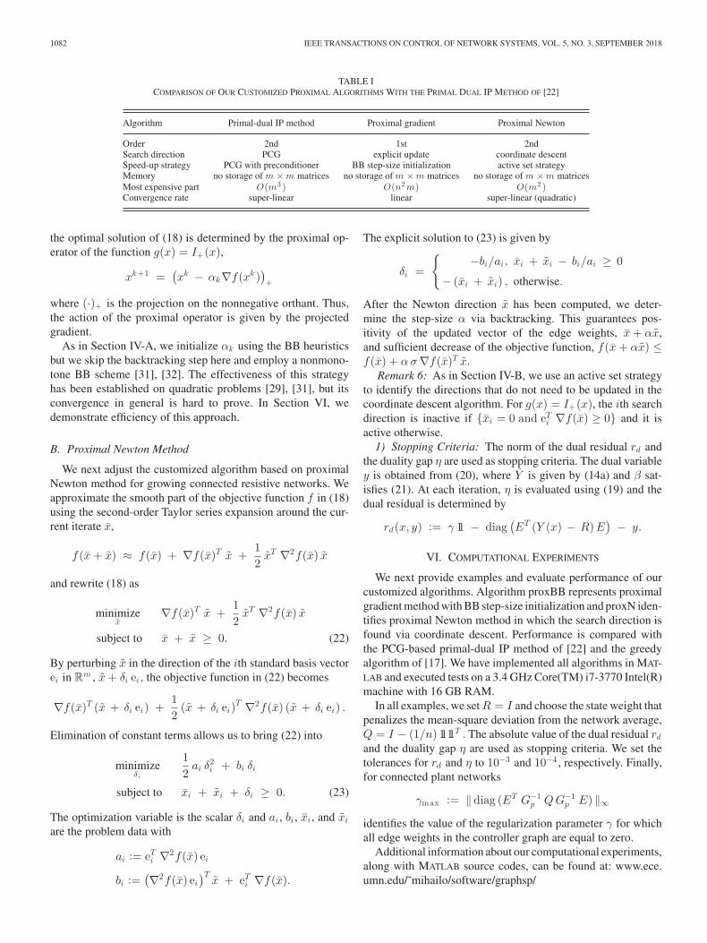
1082 IEEE TRANSACTIONS ON CONTROL OF NETWORK SYSTEMS, VOL. 5, NO. 3, SEPTEMBER 2018

TABLE ICOMPARISON OF OUR CUSTOMIZED PROXIMAL ALGORITHMS WITH THE PRIMAL DUAL IP METHOD OF [22]

Algorithm Primal-dual IP method Proximal gradient Proximal Newton

Order 2nd 1st 2ndSearch direction PCG explicit update coordinate descentSpeed-up strategy PCG with preconditioner BB step-size initialization active set strategyMemory no storage of m ×m matrices no storage of m ×m matrices no storage of m ×m matricesMost expensive part O(m3 ) O(n2m) O(m2 )Convergence rate super-linear linear super-linear (quadratic)

the optimal solution of (18) is determined by the proximal op-erator of the function g(x) = I+(x),

xk+1 =(xk − αk∇f(xk )

)+

where (·)+ is the projection on the nonnegative orthant. Thus,the action of the proximal operator is given by the projectedgradient.

As in Section IV-A, we initialize αk using the BB heuristicsbut we skip the backtracking step here and employ a nonmono-tone BB scheme [31], [32]. The effectiveness of this strategyhas been established on quadratic problems [29], [31], but itsconvergence in general is hard to prove. In Section VI, wedemonstrate efficiency of this approach.

B. Proximal Newton Method

We next adjust the customized algorithm based on proximalNewton method for growing connected resistive networks. Weapproximate the smooth part of the objective function f in (18)using the second-order Taylor series expansion around the cur-rent iterate x,

f(x+ x) ≈ f(x) + ∇f(x)T x +12xT ∇2f(x) x

and rewrite (18) as

minimizex

∇f(x)T x +12xT ∇2f(x) x

subject to x + x ≥ 0. (22)

By perturbing x in the direction of the ith standard basis vectorei in Rm , x+ δi ei , the objective function in (22) becomes

∇f(x)T (x + δi ei) +12

(x + δi ei)T ∇2f(x) (x + δi ei) .

Elimination of constant terms allows us to bring (22) into

minimizeδi

12ai δ

2i + bi δi

subject to xi + xi + δi ≥ 0. (23)

The optimization variable is the scalar δi and ai , bi , xi , and xiare the problem data with

ai := eTi ∇2f(x) ei

bi :=(∇2f(x) ei

)Tx + eTi ∇f(x).

The explicit solution to (23) is given by

δi =

{ −bi/ai, xi + xi − bi/ai ≥ 0

− (xi + xi) , otherwise.

After the Newton direction x has been computed, we deter-mine the step-size α via backtracking. This guarantees pos-itivity of the updated vector of the edge weights, x+ αx,and sufficient decrease of the objective function, f(x+ αx) ≤f(x) + ασ∇f(x)T x.

Remark 6: As in Section IV-B, we use an active set strategyto identify the directions that do not need to be updated in thecoordinate descent algorithm. For g(x) = I+(x), the ith searchdirection is inactive if {xi = 0 and eTi ∇f(x) ≥ 0} and it isactive otherwise.

1) Stopping Criteria: The norm of the dual residual rd andthe duality gap η are used as stopping criteria. The dual variabley is obtained from (20), where Y is given by (14a) and β sat-isfies (21). At each iteration, η is evaluated using (19) and thedual residual is determined by

rd(x, y) := γ 11 − diag(ET (Y (x) − R)E

) − y.

VI. COMPUTATIONAL EXPERIMENTS

We next provide examples and evaluate performance of ourcustomized algorithms. Algorithm proxBB represents proximalgradient method with BB step-size initialization and proxN iden-tifies proximal Newton method in which the search direction isfound via coordinate descent. Performance is compared withthe PCG-based primal-dual IP method of [22] and the greedyalgorithm of [17]. We have implemented all algorithms in MAT-LAB and executed tests on a 3.4 GHz Core(TM) i7-3770 Intel(R)machine with 16 GB RAM.

In all examples, we setR = I and choose the state weight thatpenalizes the mean-square deviation from the network average,Q = I − (1/n) 1111T . The absolute value of the dual residual rdand the duality gap η are used as stopping criteria. We set thetolerances for rd and η to 10−3 and 10−4 , respectively. Finally,for connected plant networks

γmax := ‖diag (ET G−1p QG−1

p E) ‖∞identifies the value of the regularization parameter γ for whichall edge weights in the controller graph are equal to zero.

Additional information about our computational experiments,along with MATLAB source codes, can be found at: www.ece.umn.edu/˜mihailo/software/graphsp/

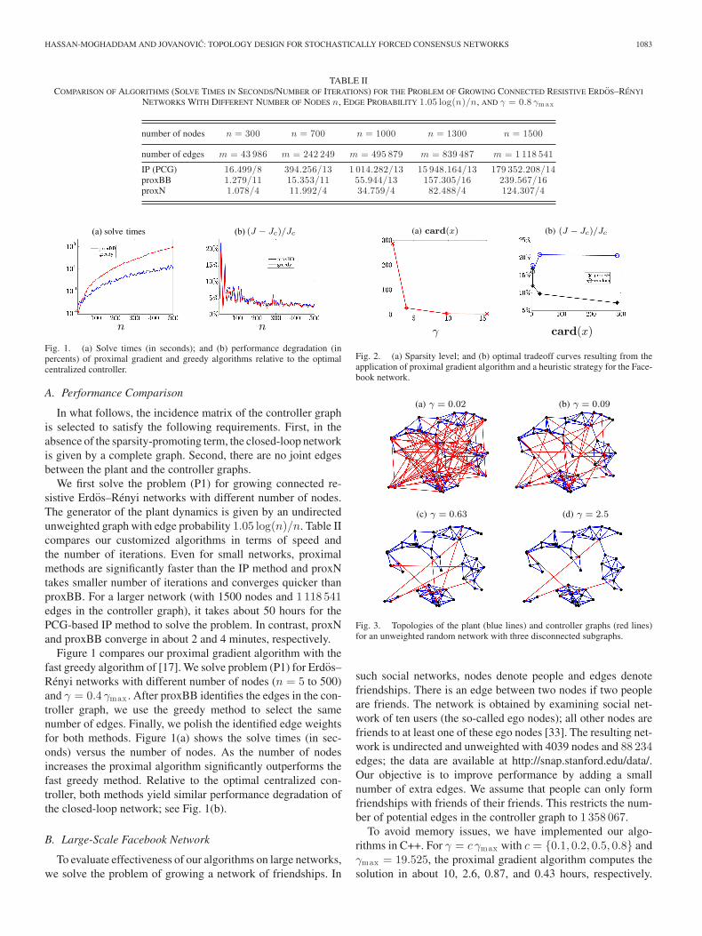
HASSAN-MOGHADDAM AND JOVANOVIC: TOPOLOGY DESIGN FOR STOCHASTICALLY FORCED CONSENSUS NETWORKS 1083

TABLE IICOMPARISON OF ALGORITHMS (SOLVE TIMES IN SECONDS/NUMBER OF ITERATIONS) FOR THE PROBLEM OF GROWING CONNECTED RESISTIVE ERDOS–RENYI

NETWORKS WITH DIFFERENT NUMBER OF NODES n, EDGE PROBABILITY 1.05 log(n)/n, AND γ = 0.8 γm ax

number of nodes n = 300 n = 700 n = 1000 n = 1300 n = 1500

number of edges m = 43 986 m = 242 249 m = 495 879 m = 839 487 m = 1 118 541

IP (PCG) 16.499/8 394.256/13 1 014.282/13 15 948.164/13 179 352.208/14proxBB 1.279/11 15.353/11 55.944/13 157.305/16 239.567/16proxN 1.078/4 11.992/4 34.759/4 82.488/4 124.307/4

Fig. 1. (a) Solve times (in seconds); and (b) performance degradation (inpercents) of proximal gradient and greedy algorithms relative to the optimalcentralized controller.

A. Performance Comparison

In what follows, the incidence matrix of the controller graphis selected to satisfy the following requirements. First, in theabsence of the sparsity-promoting term, the closed-loop networkis given by a complete graph. Second, there are no joint edgesbetween the plant and the controller graphs.

We first solve the problem (P1) for growing connected re-sistive Erdos–Renyi networks with different number of nodes.The generator of the plant dynamics is given by an undirectedunweighted graph with edge probability 1.05 log(n)/n. Table IIcompares our customized algorithms in terms of speed andthe number of iterations. Even for small networks, proximalmethods are significantly faster than the IP method and proxNtakes smaller number of iterations and converges quicker thanproxBB. For a larger network (with 1500 nodes and 1 118 541edges in the controller graph), it takes about 50 hours for thePCG-based IP method to solve the problem. In contrast, proxNand proxBB converge in about 2 and 4 minutes, respectively.

Figure 1 compares our proximal gradient algorithm with thefast greedy algorithm of [17]. We solve problem (P1) for Erdos–Renyi networks with different number of nodes (n = 5 to 500)and γ = 0.4 γmax . After proxBB identifies the edges in the con-troller graph, we use the greedy method to select the samenumber of edges. Finally, we polish the identified edge weightsfor both methods. Figure 1(a) shows the solve times (in sec-onds) versus the number of nodes. As the number of nodesincreases the proximal algorithm significantly outperforms thefast greedy method. Relative to the optimal centralized con-troller, both methods yield similar performance degradation ofthe closed-loop network; see Fig. 1(b).

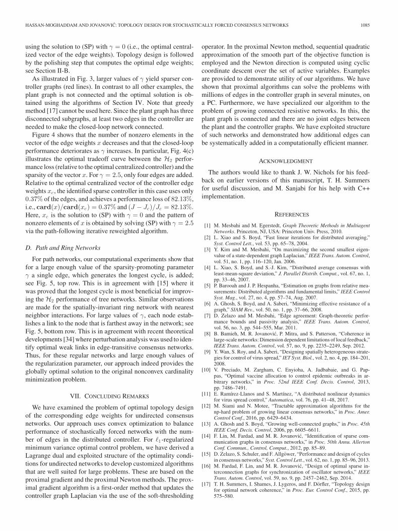
B. Large-Scale Facebook Network

To evaluate effectiveness of our algorithms on large networks,we solve the problem of growing a network of friendships. In

Fig. 2. (a) Sparsity level; and (b) optimal tradeoff curves resulting from theapplication of proximal gradient algorithm and a heuristic strategy for the Face-book network.

Fig. 3. Topologies of the plant (blue lines) and controller graphs (red lines)for an unweighted random network with three disconnected subgraphs.

such social networks, nodes denote people and edges denotefriendships. There is an edge between two nodes if two peopleare friends. The network is obtained by examining social net-work of ten users (the so-called ego nodes); all other nodes arefriends to at least one of these ego nodes [33]. The resulting net-work is undirected and unweighted with 4039 nodes and 88 234edges; the data are available at http://snap.stanford.edu/data/.Our objective is to improve performance by adding a smallnumber of extra edges. We assume that people can only formfriendships with friends of their friends. This restricts the num-ber of potential edges in the controller graph to 1 358 067.

To avoid memory issues, we have implemented our algo-rithms in C++. For γ = c γmax with c = {0.1, 0.2, 0.5, 0.8} andγmax = 19.525, the proximal gradient algorithm computes thesolution in about 10, 2.6, 0.87, and 0.43 hours, respectively.

1084 IEEE TRANSACTIONS ON CONTROL OF NETWORK SYSTEMS, VOL. 5, NO. 3, SEPTEMBER 2018

Fig. 4. (a) Sparsity level; (b) performance degradation; and (c) the optimal tradeoff curve between the performance degradation and the sparsity level of optimalsparse x compared to the optimal centralized vector of the edge weights xc . The results are obtained for unweighted random disconnected plant network withtopology shown in Fig. 3.

Fig. 5. Problems of growing unweighted path (top row) and ring (bottom row) networks. Blue lines identify edges in the plant graph, and red lines identify edgesin the controller graph.

After designing the topology of the controller graph, we opti-mize the resulting edge weights via polishing.

Figure 2(a) shows that the number of nonzero elements inthe vector x decreases as γ increases and Fig. 2(b) illustratesthat the H2 performance deteriorates as the number of nonzeroelements in x decreases. In particular, for γ = 0.8 γmax , theidentified sparse controller has only three nonzero elements (ituses only 0.0002% of the potential edges). Relative to the opti-mal centralized controller, this controller degrades performanceby 16.842%, (J − Jc)/Jc = 16.842%.

In all of our experiments, the added links with the largestedge weights connect either the ego nodes to each other or threenonego nodes to the ego nodes. Thus, our method recognizessignificance of the ego nodes and identifies nonego nodes thatplay an important role in improving performance.

We compare performance of the identified controller to aheuristic strategy that is described next. The controller graphcontains 16 potential edges between ego nodes. If the numberof edges identified by our method is smaller than 16, we ran-domly select the desired number of edges between ego nodes.Otherwise, we connect all ego nodes and select the remainingedges in the controller graph randomly. We then use polishingto find the optimal edge weights. The performance of resultingrandom controller graphs are averaged over ten trials and the

performance loss relative to the optimal centralized controlleris displayed in Fig. 2(b). We see that our algorithm alwaysperforms better than the heuristic strategy. On the other hand,the heuristic strategy outperforms the strategy that adds edgesrandomly (without paying attention to ego nodes). Unlike ourmethod, the heuristic strategy does not necessarily improve theperformance by increasing the number of added edges. In fact,the performance deteriorates as the number of edges in the con-troller graph increases from 4 to 27; see Fig. 2(b).

C. Random Disconnected Network

The plant graph (blue lines) in Fig. 3 contains 50 randomlydistributed nodes in a region of 10 × 10 units. Two nodes areneighbors if their Euclidean distance is not greater than 2 units.We examine the problem of adding edges to a plant graph whichis not connected and solve the sparsity-promoting optimal con-trol problem (SP) for controller graph with m = 1094 potentialedges. This is done for 200 logarithmically spaced values ofγ ∈ [10−3 , 2.5] using the path-following iterative reweightedalgorithm as a proxy for inducing sparsity [27]. As indicatedby (9), we set the weights to be inversely proportional to themagnitude of the solution x to (SP) at the previous value of γ.We choose ε = 10−3 in (9) and initialize weights for γ = 10−3

HASSAN-MOGHADDAM AND JOVANOVIC: TOPOLOGY DESIGN FOR STOCHASTICALLY FORCED CONSENSUS NETWORKS 1085

using the solution to (SP) with γ = 0 (i.e., the optimal central-ized vector of the edge weights). Topology design is followedby the polishing step that computes the optimal edge weights;see Section II-B.

As illustrated in Fig. 3, larger values of γ yield sparser con-troller graphs (red lines). In contrast to all other examples, theplant graph is not connected and the optimal solution is ob-tained using the algorithms of Section IV. Note that greedymethod [17] cannot be used here. Since the plant graph has threedisconnected subgraphs, at least two edges in the controller areneeded to make the closed-loop network connected.

Figure 4 shows that the number of nonzero elements in thevector of the edge weights x decreases and that the closed-loopperformance deteriorates as γ increases. In particular, Fig. 4(c)illustrates the optimal tradeoff curve between the H2 perfor-mance loss (relative to the optimal centralized controller) and thesparsity of the vector x. For γ = 2.5, only four edges are added.Relative to the optimal centralized vector of the controller edgeweights xc , the identified sparse controller in this case uses only0.37% of the edges, and achieves a performance loss of 82.13%,i.e., card(x)/card(xc) = 0.37% and (J − Jc)/Jc = 82.13%.Here, xc is the solution to (SP) with γ = 0 and the pattern ofnonzero elements of x is obtained by solving (SP) with γ = 2.5via the path-following iterative reweighted algorithm.

D. Path and Ring Networks

For path networks, our computational experiments show thatfor a large enough value of the sparsity-promoting parameterγ a single edge, which generates the longest cycle, is added;see Fig. 5, top row. This is in agreement with [15] where itwas proved that the longest cycle is most beneficial for improv-ing the H2 performance of tree networks. Similar observationsare made for the spatially-invariant ring network with nearestneighbor interactions. For large values of γ, each node estab-lishes a link to the node that is farthest away in the network; seeFig. 5, bottom row. This is in agreement with recent theoreticaldevelopments [34] where perturbation analysis was used to iden-tify optimal weak links in edge-transitive consensus networks.Thus, for these regular networks and large enough values ofthe regularization parameter, our approach indeed provides theglobally optimal solution to the original nonconvex cardinalityminimization problem.

VII. CONCLUDING REMARKS

We have examined the problem of optimal topology designof the corresponding edge weights for undirected consensusnetworks. Our approach uses convex optimization to balanceperformance of stochastically forced networks with the num-ber of edges in the distributed controller. For �1-regularizedminimum variance optimal control problem, we have derived aLagrange dual and exploited structure of the optimality condi-tions for undirected networks to develop customized algorithmsthat are well suited for large problems. These are based on theproximal gradient and the proximal Newton methods. The prox-imal gradient algorithm is a first-order method that updates thecontroller graph Laplacian via the use of the soft-thresholding

operator. In the proximal Newton method, sequential quadraticapproximation of the smooth part of the objective function isemployed and the Newton direction is computed using cycliccoordinate descent over the set of active variables. Examplesare provided to demonstrate utility of our algorithms. We haveshown that proximal algorithms can solve the problems withmillions of edges in the controller graph in several minutes, ona PC. Furthermore, we have specialized our algorithm to theproblem of growing connected resistive networks. In this, theplant graph is connected and there are no joint edges betweenthe plant and the controller graphs. We have exploited structureof such networks and demonstrated how additional edges canbe systematically added in a computationally efficient manner.

ACKNOWLEDGMENT

The authors would like to thank J. W. Nichols for his feed-back on earlier versions of this manuscript, T. H. Summersfor useful discussion, and M. Sanjabi for his help with C++implementation.

REFERENCES

[1] M. Mesbahi and M. Egerstedt, Graph Theoretic Methods in MultiagentNetworks. Princeton, NJ, USA: Princeton Univ. Press, 2010.

[2] L. Xiao and S. Boyd, “Fast linear iterations for distributed averaging,”Syst. Control Lett., vol. 53, pp. 65–78, 2004.

[3] Y. Kim and M. Mesbahi, “On maximizing the second smallest eigen-value of a state-dependent graph Laplacian,” IEEE Trans. Autom. Control,vol. 51, no. 1, pp. 116–120, Jan. 2006.

[4] L. Xiao, S. Boyd, and S.-J. Kim, “Distributed average consensus withleast-mean-square deviation,” J. Parallel Distrib. Comput., vol. 67, no. 1,pp. 33–46, 2007.

[5] P. Barooah and J. P. Hespanha, “Estimation on graphs from relative mea-surements: Distributed algorithms and fundamental limits,” IEEE ControlSyst. Mag., vol. 27, no. 4, pp. 57–74, Aug. 2007.

[6] A. Ghosh, S. Boyd, and A. Saberi, “Minimizing effective resistance of agraph,” SIAM Rev., vol. 50, no. 1, pp. 37–66, 2008.

[7] D. Zelazo and M. Mesbahi, “Edge agreement: Graph-theoretic perfor-mance bounds and passivity analysis,” IEEE Trans. Autom. Control,vol. 56, no. 3, pp. 544–555, Mar. 2011.

[8] B. Bamieh, M. R. Jovanovic, P. Mitra, and S. Patterson, “Coherence inlarge-scale networks: Dimension dependent limitations of local feedback,”IEEE Trans. Autom. Control, vol. 57, no. 9, pp. 2235–2249, Sep. 2012.

[9] Y. Wan, S. Roy, and A. Saberi, “Designing spatially heterogeneous strate-gies for control of virus spread,” IET Syst. Biol., vol. 2, no. 4, pp. 184–201,2008.

[10] V. Preciado, M. Zargham, C. Enyioha, A. Jadbabaie, and G. Pap-pas, “Optimal vaccine allocation to control epidemic outbreaks in ar-bitrary networks,” in Proc. 52nd IEEE Conf. Decis. Control, 2013,pp. 7486–7491.

[11] E. Ramırez-Llanos and S. Martınez, “A distributed nonlinear dynamicsfor virus spread control,” Automatica, vol. 76, pp. 41–48, 2017.

[12] M. Siami and N. Motee, “Tractable approximation algorithms for thenp-hard problem of growing linear consensus networks,” in Proc. Amer.Control Conf., 2016, pp. 6429–6434.

[13] A. Ghosh and S. Boyd, “Growing well-connected graphs,” in Proc. 45thIEEE Conf. Decis. Control, 2006, pp. 6605–6611.

[14] F. Lin, M. Fardad, and M. R. Jovanovic, “Identification of sparse com-munication graphs in consensus networks,” in Proc. 50th Annu. AllertonConf. Commun., Control, Comput., 2012, pp. 85–89.

[15] D. Zelazo, S. Schuler, and F. Allgower, “Performance and design of cyclesin consensus networks,” Syst. Control Lett., vol. 62, no. 1, pp. 85–96, 2013.

[16] M. Fardad, F. Lin, and M. R. Jovanovic, “Design of optimal sparse in-terconnection graphs for synchronization of oscillator networks,” IEEETrans. Autom. Control, vol. 59, no. 9, pp. 2457–2462, Sep. 2014.

[17] T. H. Summers, I. Shames, J. Lygeros, and F. Dorfler, “Topology designfor optimal network coherence,” in Proc. Eur. Control Conf., 2015, pp.575–580.

1086 IEEE TRANSACTIONS ON CONTROL OF NETWORK SYSTEMS, VOL. 5, NO. 3, SEPTEMBER 2018

[18] M. Fardad, F. Lin, and M. R. Jovanovic, “Sparsity-promoting optimalcontrol for a class of distributed systems,” in Proc. Amer. Control Conf.,2011, pp. 2050–2055.

[19] F. Lin, M. Fardad, and M. R. Jovanovic, “Design of optimal sparse feed-back gains via the alternating direction method of multipliers,” IEEETrans. Autom. Control, vol. 58, no. 9, pp. 2426–2431, Sep. 2013.

[20] J. F. Sturm, “Using SeDuMi 1.02, a MATLAB toolbox for optimiza-tion over symmetric cones,” Optim. Meth. Softw., vol. 11, no. 1–4,pp. 625–653, 1999.

[21] K.-C. Toh, M. J. Todd, and R. H. Tutuncu, “SDPT3 – A MATLAB softwarepackage for semidefinite programming, Version 1.3,” Optim. Meth. Softw.,vol. 11, no. 1–4, pp. 545–581, 1999.

[22] S. Hassan-Moghaddam and M. R. Jovanovic, “An interior point methodfor growing connected resistive networks,” in Proc. Amer. Control Conf.,Chicago, IL, USA, 2015, pp. 1223–1228.

[23] N. Parikh and S. Boyd, “Proximal algorithms,” Found. Trends Optim.,vol. 1, no. 3, pp. 123–231, 2013.

[24] A. Beck and M. Teboulle, “A fast iterative shrinkage-thresholding al-gorithm for linear inverse problems,” SIAM J. Imag. Sci., vol. 2, no. 1,pp. 183–202, 2009.

[25] J. D. Lee, Y. Sun, and M. A. Saunders, “Proximal Newton-type methodsfor minimizing composite functions,” SIAM J. Optim., vol. 24, no. 3,pp. 1420–1443, 2014.

[26] C.-J. Hsieh, M. A. Sustik, I. S. Dhillon, and P. Ravikumar, “QUIC:Quadratic approximation for sparse inverse covariance estimation,” J.Mach. Learn. Res., vol. 15, pp. 2911–2947, 2014.

[27] E. J. Candes, M. B. Wakin, and S. P. Boyd, “Enhancing spar-sity by reweighted �1 minimization,” J. Fourier Anal. Appl, vol. 14,pp. 877–905, 2008.

[28] S. Boyd and L. Vandenberghe, Convex Optimization. Cambridge, U.K.:Cambridge Univ. Press, 2004.

[29] J. Barzilai and J. M. Borwein, “Two-point step size gradient methods,”IMA J. Numer. Anal., vol. 8, no. 1, pp. 141–148, 1988.

[30] P. Tseng and S. Yun, “A coordinate gradient descent method for nonsmoothseparable minimization,” Math. Program., vol. 117, no. 1/2, pp. 387–423,2009.

[31] Y.-H. Dai and R. Fletcher, “Projected Barzilai-Borwein methods for large-scale box-constrained quadratic programming,” Numerische Math., vol.100, no. 1, pp. 21–47, 2005.

[32] S. J. Wright, R. D. Nowak, and M. A. T. Figueiredo, “Sparse reconstructionby separable approximation,” IEEE Trans. Signal Process., vol. 57, no. 7,pp. 2479–2493, Jul. 2009.

[33] J. J. McAuley and J. Leskovec, “Learning to discover social circles in egonetworks,” in Proc. Adv. Neural Inf. Process. Syst., 2012, pp. 539–547.

[34] M. Fardad, X. Zhang, F. Lin, and M. R. Jovanovic, “On the propertiesof optimal weak links in consensus networks,” in Proc. 53rd IEEE Conf.Decis. Control, 2014, pp. 2124–2129.

Sepideh Hassan-Moghaddam (S’13) received theB.Sc. degree in electrical engineering from SharifUniversity of Technology, Tehran, Iran, in 2013, andthe M.S. degree in electrical and computer engineer-ing from the University of Minnesota, Minneapolis,MN, USA, in 2016. She is currently working towardthe Ph.D. degree in the Ming Hsieh Department ofElectrical Engineering, University of Southern Cali-fornia, Los Angeles, CA, USA.

Her primary research interests include optimiza-tion, inference, and control of large-scale networks.

Mihailo R. Jovanovic (S’00–M’05–SM’13) re-ceived the Dipl. Ing. and M.S. degrees from the Uni-versity of Belgrade, Serbia, in 1995 and 1998, re-spectively, and the Ph.D. degree from the Universityof California (UC), Santa Barbara, in 2004. He is aProfessor in the Ming Hsieh Department of ElectricalEngineering and the Founding Director of the Centerfor Systems and Control at the University of South-ern California, Los Angeles, CA, USA. He was withthe faculty in the Department of Electrical and Com-puter Engineering at the University of Minnesota,

Minneapolis, MN, USA, from 2004 until 2017, and has held visiting positionswith Stanford University and the Institute for Mathematics and its Applications.He currently serves as the Chair of the APS External Affairs Committee, anAssociate Editor of the SIAM Journal on Control and Optimization, and hadserved as a Program Vice-Chair of the 55th IEEE Conference on Decision andControl and an Associate Editor of the IEEE Control Systems Society Confer-ence Editorial Board from 2006 until 2010. His research focuses on the designof controller architectures, dynamics and control of fluid flows, and fundamentalperformance limitations in the design of large dynamic networks.

Prof. Jovanovic received a CAREER Award from the National Science Foun-dation in 2007, the George S. Axelby Outstanding Paper Award from the IEEEControl Systems Society in 2013, and the Distinguished Alumni Award from theDepartment of Mechanical Engineering at UC Santa Barbara in 2014. Papersof his students were finalists for the Best Student Paper Award at the AmericanControl Conference in 2007 and 2014.