Topology of the Magnetic Domains of a Co/Pt Multilayer

Topology of the Magnetic Domains of a Co/Pt Multilayer

with 16Å Cobalt Layers

Matthew Healey

A capstone report submitted to the faculty of

Brigham Young University

In partial fulfillment of the requirements for the degree of

Bachelor of Science

Dr. Karine Chesnel, Advisor

Department of Physics and Astronomy

Brigham Young University

June 10, 2016

© 2016 Matthew Healey

All Rights Reserved

i

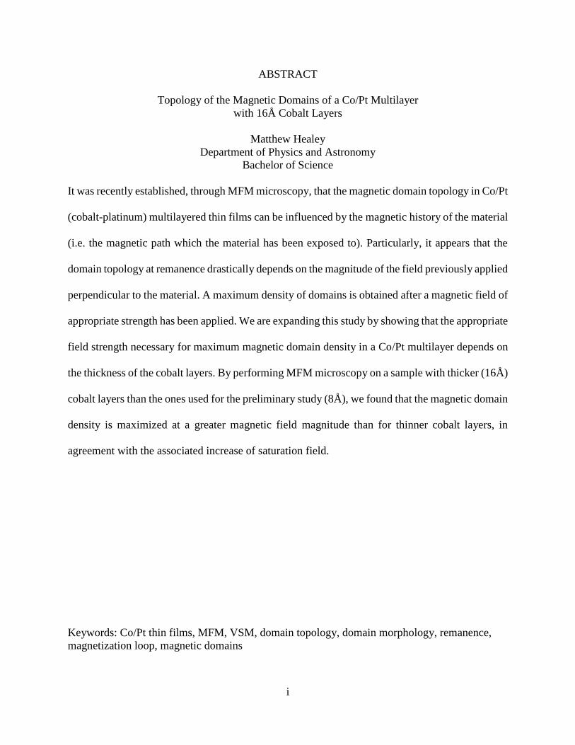
ABSTRACT

Topology of the Magnetic Domains of a Co/Pt Multilayer

with 16Å Cobalt Layers

Matthew Healey

Department of Physics and Astronomy

Bachelor of Science

It was recently established, through MFM microscopy, that the magnetic domain topology in Co/Pt

(cobalt-platinum) multilayered thin films can be influenced by the magnetic history of the material

(i.e. the magnetic path which the material has been exposed to). Particularly, it appears that the

domain topology at remanence drastically depends on the magnitude of the field previously applied

perpendicular to the material. A maximum density of domains is obtained after a magnetic field of

appropriate strength has been applied. We are expanding this study by showing that the appropriate

field strength necessary for maximum magnetic domain density in a Co/Pt multilayer depends on

the thickness of the cobalt layers. By performing MFM microscopy on a sample with thicker (16Å)

cobalt layers than the ones used for the preliminary study (8Å), we found that the magnetic domain

density is maximized at a greater magnetic field magnitude than for thinner cobalt layers, in

agreement with the associated increase of saturation field.

Keywords: Co/Pt thin films, MFM, VSM, domain topology, domain morphology, remanence,

magnetization loop, magnetic domains

ii

ACKNOWLEDGMENTS

I thank Dr. Karine Chesnel for her confidence, training, motivation, qualifications, and dedication

to helping me succeed. I thank Berg Dodson for collaborating with Dr. Chesnel in order to train

me quickly and efficiently; I also thank Berg for the work that he has done on other Co/Pt samples.

I thank Phillip Salter, who designed the software used for the analysis of the MFM images. I finally

express appreciation and thanks to my wife, without whom I wouldn’t have been able to complete

this project.

iii

Table of Contents

Abstract ............................................................................................................................................ i

Acknowledgments........................................................................................................................... ii

Table of Contents ........................................................................................................................... iii

Table of Figures ............................................................................................................................. iv

1. Introduction ..................................................................................................................................1

2. Methods........................................................................................................................................2

2.1 Overview ...............................................................................................................................2

2.2 VSM Technique ....................................................................................................................3

2.3 MFM Technique ...................................................................................................................7

2.4 Magnetic Image Analysis ...................................................................................................10

3. Results and Discussion ..............................................................................................................12

4. Conclusion .................................................................................................................................17

References ......................................................................................................................................19

iv

Table of Figures

Figure 1—PPMS and VSM Setup ...................................................................................................4

Figure 2—Magnetization Loops ......................................................................................................5

Figure 3— Magnetization Loops .....................................................................................................5



Figure 6—AFM Diagram ................................................................................................................8

Figure 7—10 × 10 μm2 AFM/MFM Image (Hm = 2.00 T) ..........................................................9

Figure 8—Black and White MFM Image ......................................................................................11

Figure 9—[Co(16Å)/Pt(7Å)]50 Remanent MFM Images (Hm from 9 T to 0.8 T) ........................13

Figure 10—[Co(16Å)/Pt(7Å)]50 Remanent MFM Images (Hm from 0.75 T to 0.3 T) .................14

Figure 11—[Co(16Å)/Pt(7Å)]50 Remanent MFM Images (Hm from 0.2 T to 0.1 T) ...................15

Figure 12—Magnetic Domain Density vs Hm ...............................................................................16

Figure 13—Magnetic Domain Density vs Hm (Hm from 4,500 Oe to 10,000 Oe) ......................16

1

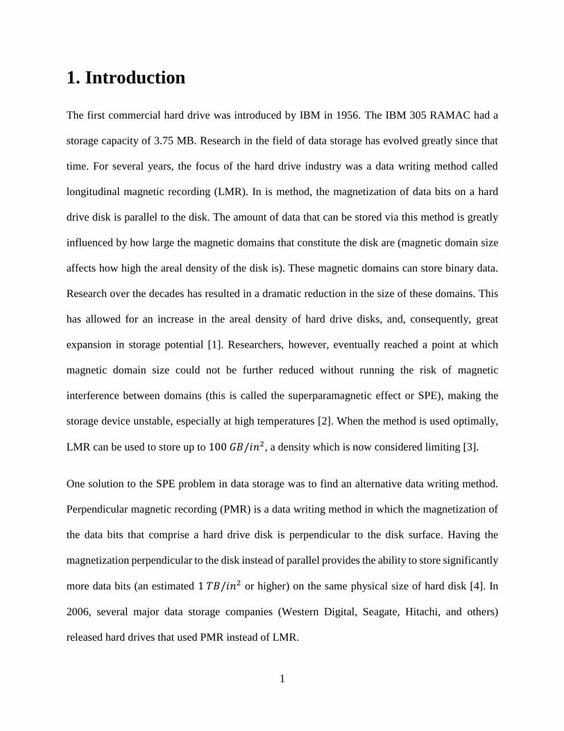
1. Introduction

The first commercial hard drive was introduced by IBM in 1956. The IBM 305 RAMAC had a

storage capacity of 3.75 MB. Research in the field of data storage has evolved greatly since that

time. For several years, the focus of the hard drive industry was a data writing method called

longitudinal magnetic recording (LMR). In is method, the magnetization of data bits on a hard

drive disk is parallel to the disk. The amount of data that can be stored via this method is greatly

influenced by how large the magnetic domains that constitute the disk are (magnetic domain size

affects how high the areal density of the disk is). These magnetic domains can store binary data.

Research over the decades has resulted in a dramatic reduction in the size of these domains. This

has allowed for an increase in the areal density of hard drive disks, and, consequently, great

expansion in storage potential [1]. Researchers, however, eventually reached a point at which

magnetic domain size could not be further reduced without running the risk of magnetic

interference between domains (this is called the superparamagnetic effect or SPE), making the

storage device unstable, especially at high temperatures [2]. When the method is used optimally,

LMR can be used to store up to 100 𝐺𝐵/𝑖𝑛2, a density which is now considered limiting [3].

One solution to the SPE problem in data storage was to find an alternative data writing method.

Perpendicular magnetic recording (PMR) is a data writing method in which the magnetization of

the data bits that comprise a hard drive disk is perpendicular to the disk surface. Having the

magnetization perpendicular to the disk instead of parallel provides the ability to store significantly

more data bits (an estimated 1 𝑇𝐵/𝑖𝑛2 or higher) on the same physical size of hard disk [4]. In

2006, several major data storage companies (Western Digital, Seagate, Hitachi, and others)

released hard drives that used PMR instead of LMR.

2

Research in materials that could further optimize the use of PMR in data storage has continued to

this day. Multi-layer Co/Pt thin films exhibit perpendicular magnetic anisotropy, and are a

promising material [5]. Perpendicular magnetic domains naturally form in this material, even in

the absence of a magnetic field. The morphology of these domains at remanence, however, appears

to depend on magnetic history. The morphology of these domains is of great interest in the data

storage industry, for they determine the density of data bytes that could be stored. A study of Co/Pt

thin films was undertaken by Dr. Karine Chesnel and some of her associates. Particularly, they

focused on [Co(8Å)/Pt(7Å)]50 (i.e. a Co/Pt multilayer thin film with 8 Å of cobalt layered on 7 Å

of platinum 50 times) [6]. They found that magnetic domain density can be influenced when the

material is previously magnetized to a critical level (somewhat before saturation). This

measurement was carried at remanence (residual magnetism after the external magnetic field is

brought back to zero). This report summarizes my efforts to contribute to the exploration of how

the morphology and density of these magnetic domains depends on magnetic history (in this case,

which fields have been applied before remanence) for a sample with thicker cobalt layers

([Co(16Å)/Pt(7Å)]50).

2. Methods

2.1 Overview

A series of magnetization loops were applied perpendicularly to the [Co(16Å)/Pt(7Å)]50 film using

vibrating sample magnetometer (VSM) technique. Our VSM is part of a Quantum Design physical

property measurement system (PPMS). After each magnetization loop was applied, a magnetic

image was taken of the sample at remanence via magnetic force microscopy (MFM). These images

provide information pertaining to the density and topology of the magnetic domains. A custom-

3

made program, called Magnetic Image Analyzer (MIA), enabled us to statistically analyze each of

the MFM images.

2.2 VSM Technique

The PPMS instrument uses a superconducting magnet to produce a magnetic field of desired

strength (up to 9 𝑇). The superconducting magnet functions as follows: first, a power supply injects

a current into the circuit; second, a persistent switch, which is a small portion of the

superconducting magnet wire, gets heated by a resistive wire, causing the magnet controller to

enter the superconducting circuit; third, a magnet controller drives the magnet to the current

required for a higher magnetic field. The persistent switch heater is then turned off, and the process

repeats itself until the desired magnetic field value is reached [7].

While a magnetization loop is being applied to a sample, the VSM enables us to track the magnetic

moment 𝑀 (see Figure 1). The VSM accesses the magnetic moment 𝑀 by exploiting the Faraday

effect, i.e. the fact that a changing magnetic flux will induce a voltage in a pickup coil:

𝑉𝑒𝑚𝑓 = −𝜕Φ

𝜕𝑡 ,

where 𝑉𝑒𝑚𝑓 is electromagnetic force and Φ is magnetic flux. As the name suggests, the vibrating

sample magnetometer causes a sample to oscillate vertically near a pickup coil; this sinusoidal

motion results in a changing magnetic flux and induced voltage. The voltage across the pickup

coil is easily measured, and the following formula can be used to determine the magnetic

moment of the sample:

𝑀 =𝑉𝑐𝑜𝑖𝑙

2𝜋𝑓𝐶𝐴𝑠𝑖𝑛(2𝜋𝑓𝑡) ,

4

where 𝑉𝑐𝑜𝑖𝑙 is voltage in the pickup coil, 𝑓 is the frequency of oscillation (40 𝐻𝑧), 𝐶 is a coupling

constant, 𝐴 is the amplitude of oscillation (1– 3 𝑚𝑚), and 𝑡 is time [8]. Ultimately, we measure

the magnetic moment 𝑀 as a function of various parameters such as time 𝑡, temperature 𝑇, and

magnetic field 𝐻. Our focus is primarily on magnetic moment as a function of magnetic field

𝑀(𝐻) throughout our magnetization loop measurements.

Figure 1—The PPMS and VSM setup. The VSM is located at position ❶; samples are mounted through the top of

the device and inserted inside the PPMS superconducting magnet, which is located at position ❷. The pickup coils

to perform VSM measurements are mounted before a sample is inserted. A CRYOMECH PT410 helium compressor

is located at ❸ to efficiently use the liquid helium needed for the superconducting components of the PPMS. A

reservoir of liquid helium is located at ❹.

❶

❷

❸

❹

5

Figure 2—Magnetic moment of [Co(16Å)/Pt(7Å)]50 as a function of magnetic field for the magnetization loops with

a magnitude of 9.00 T, 5.00 T, 2.00 T, 1.50 T, and 1.00 T.


a magnitude of 0.95 T, 0.90 T, 0.85 T, 0.80 T, and 0.75 T. The saturation field magnitude, 𝐻𝑠 = 0.85 𝑇, is apparent.

6





7

The [Co(16Å)/Pt(7Å)]50 sample was kept at room temperature while the magnetization loops were

applied to it during VSM measurements. My work focused on applying a series of magnetization

loops with decreasing magnitude (a descending series). The first magnetization loop in the

descending series had a magnetic field magnitude of 9.0 T (the sample was brought back down to

remanence at the end of each magnetization loop). The last magnetic field applied to the sample

had a magnitude of 0.1 T. Figures 2–5 show the magnetic moment of our sample as a function of

magnetic field for each of the twenty magnetization loops that were applied to our sample

throughout the course of the project.

2.3 MFM Technique

Magnetic force microscopy (MFM) is done simultaneously with atomic force microscopy (AFM).

AFM is a scanning microscope in which a small tip at the end of a cantilever is moved across the

surface of a sample, line by line, to generate an image of physical topography. This is possible

because of the Van-der-Waals forces between the tip and the surface of the sample. These forces

cause deflection in the cantilever attached to the tip. These deflections are measured by reflecting

a laser beam off of the cantilever onto a position sensitive photodiode (PSPD); physical topography

can be determined based on the readings of the PSPD (see Figure 6) [9]. We use tapping mode for

our imaging, so the tip vibrates at its resonant frequency (typically 80– 95 𝑘𝐻𝑧) while moving

across our samples line by line. Figure 7 (a) shows an example of an AFM image.

8

Figure 6—Basic diagram of how atomic force microscopy is performed. A laser beam is reflected off of the top of

the cantilever onto a PSPD. As the tip moves across the sample surface, the atomic force between the sample and the

tip cause the cantilever to deflect, which moves the laser to a different position on the PSPD. The PSPD readings are

used to map out the topography of the sample.

9

Figure 7—(a) A 10 × 10 𝜇𝑚2 AFM image of [Co(16Å)/Pt(7Å)]50. (b) A 10 × 10 𝜇𝑚2 MFM image of

[Co(16Å)/Pt(7Å)]50 taken at remanence after a magnetization loop with a magnitude of 2.0 T was applied (𝐻𝑚 =2.0 𝑇).

For MFM to be performed, the tip mounted on a cantilever must first be magnetized. After an

AFM line is recorded, the microscope head is lifted to a height, typically 40– 70 𝑛𝑚, above the

sample. Once lifted, the tip is moved across the sample again on the same line, retracing the

topography that was just measured via AFM. If the material being scanned exhibits perpendicular

magnetic stray fields, the tip will be deflected via magnetic interaction with the sample. This

deflection causes a phase difference between the path recorded during the AFM line and the path

recorded during the MFM line. This phase difference is recorded on the PSPD, which determines

whether the tip was attracted to the sample or repelled away from the sample for all points along

the line. This information yields an image of the magnetic domains present in the sample [10].

Figure 7 (b) displays an example of a MFM image. Magnetic domains, areas of the sample that

are magnetized in the same direction, are indicated on the MFM image by regions of the same

color (either yellow or brown): the brown signifies magnetization opposite the previously applied

10

field, while the yellow signifies magnetization aligned with the previously applied field. If the

sample were saturated, not at remanence, then no domains would remain, and a MFM image would

appear purely yellow.

A 10 × 10 𝜇𝑚2 MFM image was taken of our [Co(16Å)/Pt(7Å)]50 sample after each of the twenty

magnetization loops were applied. These images hold information pertaining to the morphology

and density of magnetic domains of our Co/Pt samples.

2.4 Magnetic Image Analysis

The MIA program allows us to determine the number of each type of magnetic domains that are

present in our MFM images (pointing out of or into the sample), and, thus, the density of magnetic

domains throughout our sample (for each of the magnetization loops applied). The program also

computes the size of each magnetic domain in our images, the average domain size throughout the

sample, and the net magnetization of our sample. Without such a program, quantitative analysis of

our MFM images would be nearly impossible. The MIA accomplishes all this through four simple

steps:

1. Binary rendering of the MFM image (see Figure 8)—while the program is running, the

user is prompted to enter a cutoff value between 0 and 250 (0 corresponds to all white and

250 corresponds to all black). All pixels in the image that have a value lower than the

cutoff entered by the user are converted into white pixels (up or +), while those with a

value higher than the one entered are converted into black pixels (down or −).

11

Figure 8—A portion of the MFM image displayed in Figure 7 that has been rendered black and white by the MIA

program. White represents upward pointing magnetic domains; black represents downward pointing magnetic

domains.

2. Listing the domains—the program scans the image from right to left and top to bottom,

counting the clusters of pixels that are surrounded by pixels of the opposite color. The

domains are listed along with their sizes (in pixels).

3. Counting the domains—from the list of domains and sizes, the program counts the total

number of domains pointing up and down (𝐷+ and 𝐷−, respectively), the total number of

up and down pixels (𝑁+ and 𝑁−, respectively), and the average domain area (𝑆+ and 𝑆−).

𝑆+ =𝑁+

𝐷+ and 𝑆− =

𝑁−

𝐷− .

4. Calculating net magnetization—based on the information found in step three, the program

determines a normalized net magnetization of the sample, 𝑀, through the following

equation:

𝑀 =𝑁+ − 𝑁−

𝑁+ + 𝑁− .

12

𝑀 is normalized such that −1 ≤ 𝑀 ≤ 1: 𝑀 = −1 when 𝑁+ = 0, and 𝑀 = 1 when 𝑁− = 0. The

user-input value described in step one is chosen such that the net magnetization calculated in step

four matches that of the sample after the applied magnetization loop as experimentally measured.

As can be seen in Figures 2–5, after each magnetization loop is applied, the net magnetic moment

of [Co(16Å)/Pt(7Å)]50 is slightly above zero once remanence is reached 𝑀 ≅ 0.

3. Results and Discussion

As indicated in Figure 3, the saturation field magnitude for [Co(16Å)/Pt(7Å)]50 is 𝐻𝑠 = 0.85 𝑇,

which is higher than that of [Co(8Å)/Pt(7Å)]50 (𝐻𝑠 = 0.60 𝑇) [6]. This leads us to anticipate that

the magnetic field magnitude, 𝐻∗, necessary to maximize the magnetic domain density of

[Co(16Å)/Pt(7Å)]50 is also greater than that of [Co(8Å)/Pt(7Å)]50 (𝐻∗ = 0.5 𝑇). MFM images

corresponding to each of the twenty applied magnetization loops applied to [Co(16Å)/Pt(7Å)]50

are displayed below in Figures 9–11 (note that 𝐻𝑚 is the magnitude of the field previously applied).

13

[Co(16Å)/Pt(7Å)]50 Remanent MFM Images

Figure 9—10 × 10 𝜇𝑚2 MFM images of [Co(16Å)/Pt(7Å)]50 taken at remanence for indicated 𝐻𝑚 from 9 𝑇–0.8 𝑇

14


Figure 10—10 × 10 𝜇𝑚2 MFM images of [Co(16Å)/Pt(7Å)]50 taken at remanence for indicated 𝐻𝑚 from 0.75 𝑇–

0.3 𝑇

15


Figure 11—10 × 10 𝜇𝑚2 MFM images of [Co(16Å)/Pt(7Å)]50 taken at remanence for indicated 𝐻𝑚 from 0.2 𝑇–

0.1 𝑇

In the first few MFM images, both the downward pointing and upward pointing magnetic domains

take on a maze-like structure (Figure 9, 𝐻𝑚 from 9 𝑇–0.9 𝑇). As the magnitude of the

magnetization loops applied becomes lower than the value necessary to saturate

[Co(16Å)/Pt(7Å)]50, the downward pointing domains (the dark domains) begin to shrink in length.

This occurs because, since the sample does not get fully saturated, the domains that oppose the

direction of the applied magnetic field do not entirely collapse once the magnetic field reaches its

highest value 𝐻𝑚; their presence prevents the magnetic domains that form while the magnetic field

approaches remanence from becoming long and maze-like [6]. The result is a greater density of

smaller magnetic domains for several magnetization loops (Figure 9 and Figure 10, 𝐻𝑚

from 0.85 𝑇–0.65 𝑇). As the magnitude of 𝐻𝑚 decreases further below that point, the density of

downward-pointing magnetic domains decreases, and the dark domains extend in length and return

to a maze-like structure (Figures 9–11, 𝐻𝑚 from 0.6 𝑇–0.1 𝑇).

Although difficult to detect with the naked eye on the MFM image, the density of downward

pointing magnetic domains in [Co(16Å)/Pt(7Å)]50 clearly reaches a peak at an optimizing field

magnitude in the descending series of magnetization loops. Figure 12 and Figure 13 show plots of

16

the number of both types of magnetic domains as a function of the maximum magnetic field 𝐻𝑚

of the previously applied magnetization loop.

Figure 12—Plot of the number of upward and downward pointing magnetic domains per 100 𝜇𝑚2 as a function of

the magnitude of the previously applied magnetization loop (𝐻𝑚).

Figure 13—Zoom of Figure 12, displaying the 4,500–10,000 𝑂𝑒 region.

As was the case for [Co(8Å)/Pt(7Å)]50, the magnetic domain density of [Co(16Å)/Pt(7Å)]50 can

be optimized by adjusting the previously applied magnetic field. The magnetic domain density of

17

[Co(16Å)/Pt(7Å)]50 was maximized to above 550 domains/100 𝜇𝑚2, nearly five times the initial

domain density, after a magnetization loop with a magnitude of 𝐻𝑚 = 𝐻∗ = 7,500 𝑂𝑒 was applied

to the sample (for [Co(8Å)/Pt(7Å)]50, it was maximized at 𝐻∗ = 5,000 𝑂𝑒). For both

[Co(8Å)/Pt(7Å)]50 and [Co(8Å)/Pt(7Å)]50, 𝐻∗ is somewhat lower than the respective saturation

field 𝐻𝑠 (𝐻∗ < 𝐻𝑠. The maximum density of downward pointing magnetic domains that were

found in [Co(16Å)/Pt(7Å)]50 was ~565 per 100 𝜇𝑚2 (compared with ~600 per 100 𝜇𝑚2 for

[Co(8Å)/Pt(7Å)]50) [6].

4. Conclusion

Remanent magnetic domain density for [Co(16Å)/Pt(7Å)]50 is maximized at a field magnitude of

𝐻∗ = 7,500 𝑂𝑒. This field strength is greater than that of [Co(8Å)/Pt(7Å)]50 in agreement with the

increase in saturation field 𝐻𝑠. We thus conclude that the magnitude of the magnetization loop that

is needed to maximize magnetic domain density in a Co/Pt multilayer sample seems to increase

with the thickness of the cobalt layers in the material. Research is currently underway with samples

that have 4 Å, 12 Å, 25 Å, 31 Å, 40 Å, and 60 Å thick cobalt layers. Once we determine at which

magnetic field magnitudes these samples exhibit a maximum density of magnetic domains, we

will be in a position to map out the relationship between the thickness of cobalt layers and the

magnetic field necessary to maximize the density of magnetic domains in Co/Pt multilayers.

The measured maximum density of downward pointing magnetic domains attained at the

optimizing magnetization loop for [Co(16Å)/Pt(7Å)]50 was approximately 565 per 100 𝜇𝑚2. This

number could possibly be further increased by using higher resolution around the peak for the 16Å

sample. In the future we will revisit [Co(16Å)/Pt(7Å)]50 and apply fields from 8,000 𝑂𝑒 to

7,000 𝑂𝑒 at intervals of 100 𝑂𝑒, analyzing the density of downward pointing magnetic domains.

18

This will help us determine whether cobalt layer thickness also correlates with the maximum

density of downward pointing magnetic domains in addition to peak location.

19

References

[1] Perpendicular magnetic recording (PMR). Lake Forest, CA: Western Digital

Technologies (2006).

[2] Kryder, M. H. Magnetic recording beyond the superparamagnetic limit. 2000 IEEE

International, 1, 575 (2000).

[3] Weller, D., & Doerner, M. F. Extremely high-density longitudinal magnetic recording

media. Annual Review of Materials Science, 30, 611 (2000).

doi:10.1146/annurev.matsci.30.1.611

[4] Khizroev, S. In Dmitri Litvinov, SpringerLink (Online service) and by Sakhrat Khizroev D.

L. (Eds.), Perpendicular magnetic recording Springer Netherlands, Dordrecht (2005).

[5] Hwang, P., Li, B., Yant, T., & Zhu, F. Perpendicular magnetic anisotropy of Co85Cr15/Pt

multilayers. Journal of University of Science and Technology Beijing, 11(4), 319-323 (2004).

[6] Westover, A., Chesnel, K., Hatch, K., Salter, P., & Hellwig, O. Enhancement of magnetic

domain topologies in Co/Pt thin film by fine tuning magnetic field path throughout hysteresis

loop. Journal of Magnetism and Magnetic Materials, 399, 164 (2016).

doi:10.1016/j.jmmm.2015.09.040

[7] Physical property measurement system hardware manual, 6th ed. (Quantum Design, San

Diego, CA) 45 (2008).

[8] Vibrating sample magnetometer (VSM) option User’s manual, 5th ed. (Quantum Design, San

Diego, CA) 18 (2011).

[9] Atomic force microscopy (AFM), In H. Yang (Eds.), (Nova Science Publishers, Inc.,

Hauppauge, NY) 57 (2014).

[10] Ferri, F. A., Pereira, M. A., & Marega Jr., E. Magnetic force microscopy: Basic principles

and applications. In V. Bellitto (Ed.), Atomic force microscopy - imaging, measuring and

manipulating surfaces at the atomic scale (Rijeka, Croatia: InTech) 39 (2012).

Documents

Topology of the Magnetic Domains of a Co/Pt Multilayer