TOPOLOGY OPTIMIZATION OF CONVECTIVE - Deep Blue

TOPOLOGY OPTIMIZATION OF CONVECTIVE COOLING

SYSTEM DESIGNS

by

Kyungjun Lee

A dissertation submitted in partial fulfillment

of the requirements for the degree of

Doctor of Philosophy

(Mechanical Engineering)

in The University of Michigan

2012

Doctoral Committee:

Professor Noboru Kikuchi, Chair

Professor Greg Hulbert

Professor Kenneth G. Powell

Research Scientist Zheng-Dong Ma

© Kyungjun Lee

2012

ii

DEDICATION

To my family

iii

ACKNOWLEDGEMENTS

I would like to express my appreciation to my advisor, Professor Noboru Kikuchi for

his gentle guidance, great inspiration and financial support during my doctoral studies at

the University of Michigan. I also would like to sincerely acknowledge the helpful

suggestions and criticisms made by my doctoral committee members, Professor Kenneth

G. Powell, Professor Gregory M. Hulbert, Professor Kazuhiro Saitou and Dr. Zheng-

Dong Ma. I would like to express my gratitude to Professor Yoon Young Kim and

Professor Seungjae Min, for their guidance and advice in my research.

I wish to express my special thanks to Dr. Jeong Hun Seo, Dr. Jaewook Lee and Dr.

Youngwon Hahn, who gave me a great help when studying the fundamental of topology

optimization theory, for their kindness and friendship. My special thanks are expressed to

Dr. Huerta Jill and Dr. Roann Altman for their tutoring me with writing in English.

Finally, I am grateful to my family and all my friends who physically and mentally

support me to get through difficult times. This work would not have been possible

without the support and encouragement of my parents, my sisters, and many others with

whom I shared memories during my studies in Ann Arbor.

iv

TABLE OF CONTENTS

DEDICATION .............................................................................................................. ii

ACKNOWLEDGEMENTS ........................................................................................ iii

LIST OF FIGURES ................................................................................................... vii

LIST OF TABLES ..................................................................................................... xii

ABSTRACT ............................................................................................................... xiii

CHAPTER

1. INTRODUCTION .................................................................................................... 1

1.1. Motivation and goal ............................................................................................. 1

1.2. Cooling system design optimization .................................................................... 4

1.3. Topology optimization of thermal-fluid cooling system ..................................... 8

1.4. Stabilized finite element method ....................................................................... 11

1.5. Outline of dissertation ........................................................................................ 13

2. THERMAL-FLUID ANALYSIS FOR TOPOLOGY OPTIMIZATION ......... 14

v

2.1. Introduction ........................................................................................................ 14

2.2. Governing equations for topology optimization ................................................ 15

2.3. Stabilized finite element method ....................................................................... 24

2.4. Newton-Raphson method ................................................................................... 31

2.5. Numerical issues ................................................................................................ 38

2.6. Summary ............................................................................................................ 53

3. TOPOLOGY OPTIMIZATION OF NAVIER-STOKES FLOW

PROBLEMS ............................................................................................................ 55

3.1. Introduction ........................................................................................................ 55

3.2. Sensitivities analysis for nonlinear problems .................................................... 56

3.3. Numerical issues ................................................................................................ 63

3.4. Design of Navier-Stokes flow systems .............................................................. 86

3.5. Summary ............................................................................................................ 95

4. TOPOLOGY OPTIMIZATION OF CONVECTIVE COOLING SYSTEMS . 97

4.1. Introduction ........................................................................................................ 97

4.2. Sensitivity analysis for multiphysics problems .................................................. 98

4.3. Numerical issues .............................................................................................. 105

4.4. Design of thermal-fluid cooling system ........................................................... 118

4.5. Summary .......................................................................................................... 128

5. CONCLUSION ..................................................................................................... 130

5.1. Concluding remarks ......................................................................................... 130

5.2. Future works .................................................................................................... 133

APPENDIX ............................................................................................................... 136

vi

BIBLIOGRAPHY .................................................................................................... 143

vii

LIST OF FIGURES

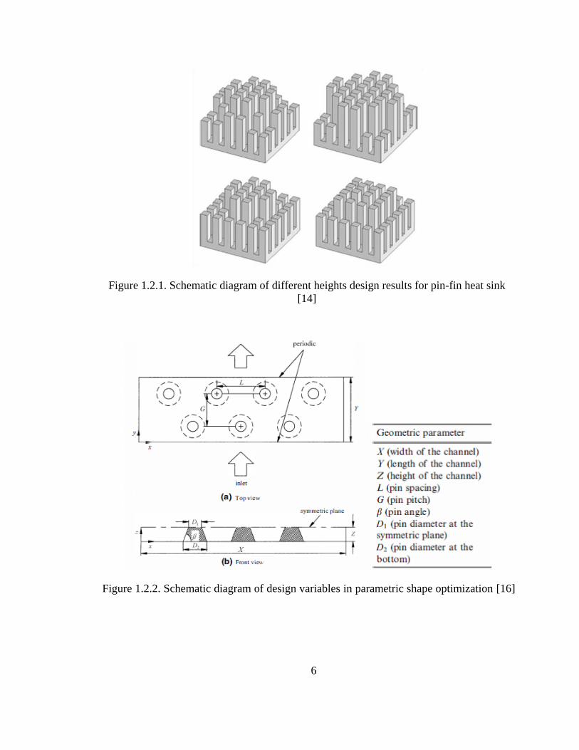
Figure 1.2.1. Schematic diagram of different heights design results for pin-fin heat sink

[14] ...................................................................................................................................... 6

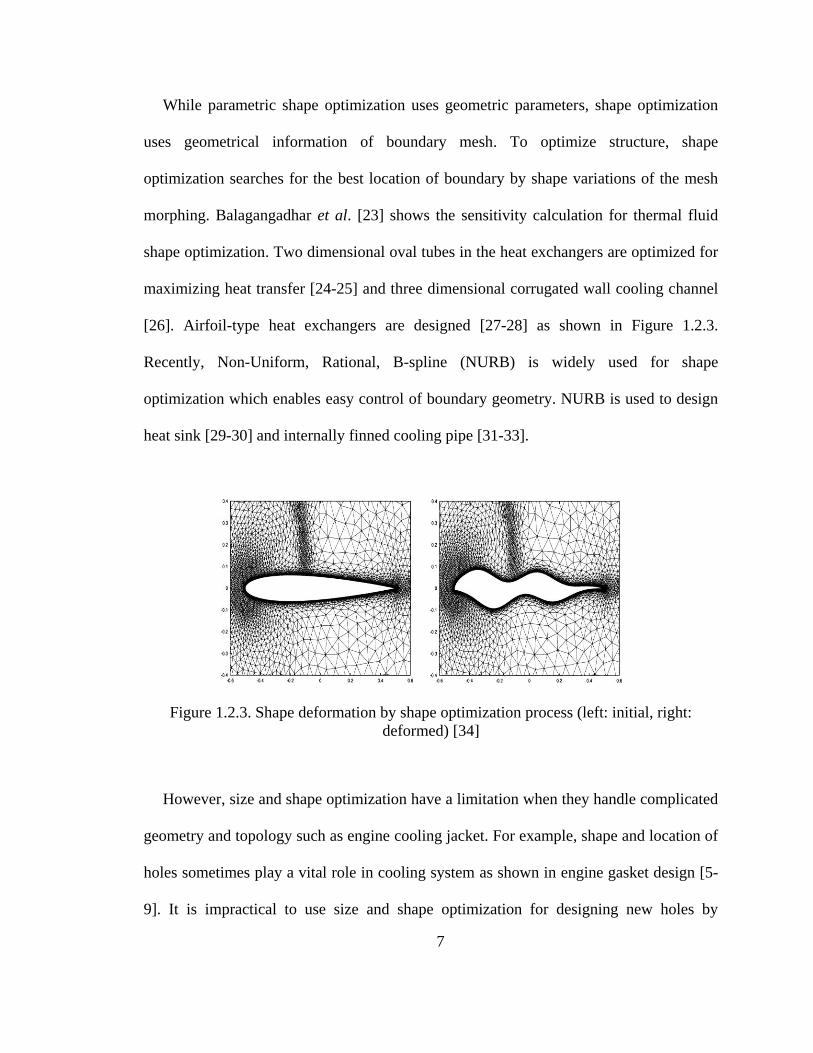
Figure 1.2.2. Schematic diagram of design variables in parametric shape optimization

[16] ...................................................................................................................................... 6

Figure 1.2.3. Shape deformation by shape optimization process (left: initial, right:

deformed) [34] .................................................................................................................... 7

Figure 2.2.1. Fluid-solid system in topology optimization for fluid systems ................... 16

Figure 2.2.2. Representation of the solid region as a porous medium [42] ...................... 16

Figure 2.4.1. Flow chart of the Reynolds-ramping initial guess ....................................... 33

Figure 2.4.2. 2D lid-driven cavity problems [P1] with no-slip boundary [P2] with solid

region and immersed boundary ......................................................................................... 36

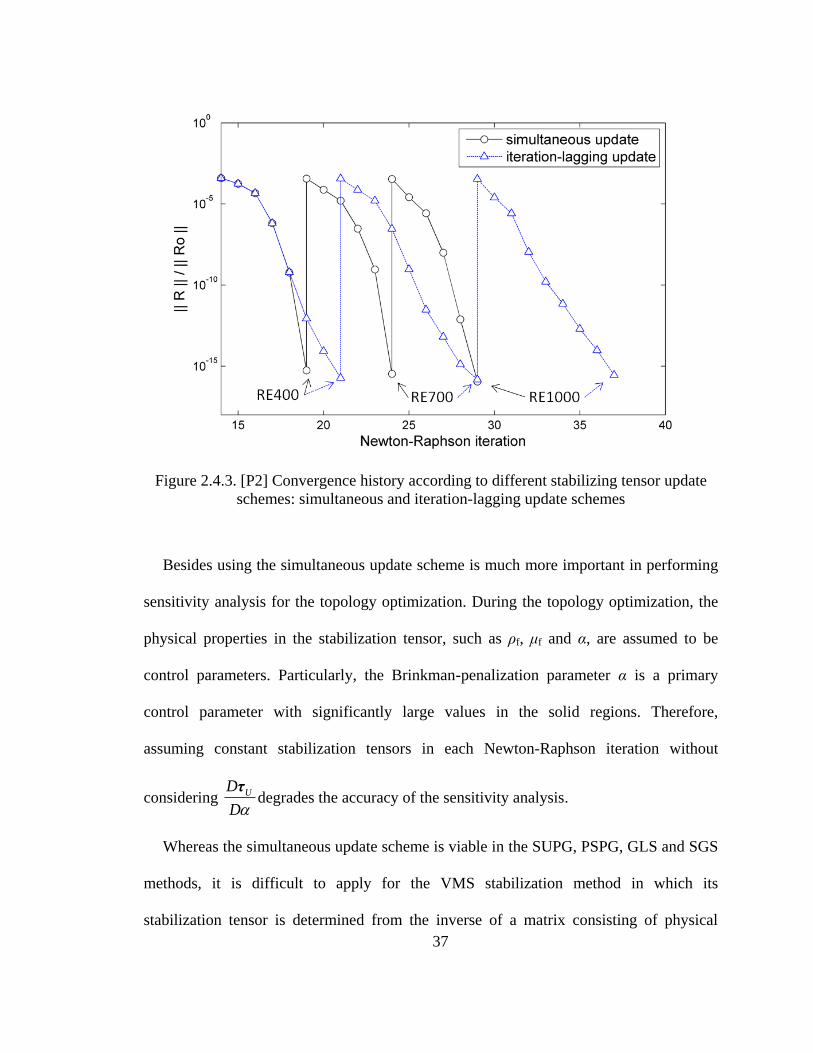
Figure 2.4.3. [P2] Convergence history according to different stabilizing tensor update

schemes: simultaneous and iteration-lagging update schemes ......................................... 37

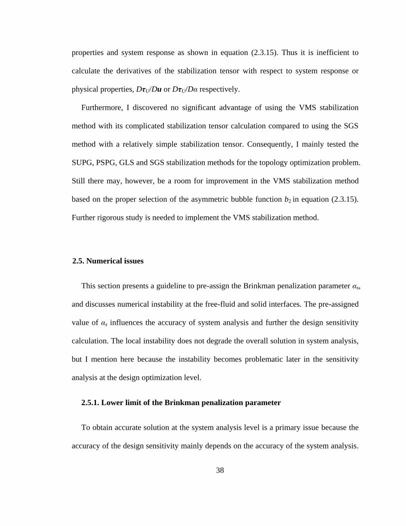
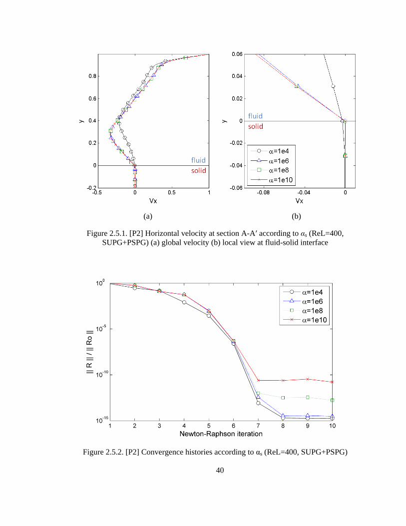
Figure 2.5.1. [P2] Horizontal velocity at section A-A′ according to αs (ReL=400,

SUPG+PSPG) (a) global velocity (b) local view at fluid-solid interface ......................... 40

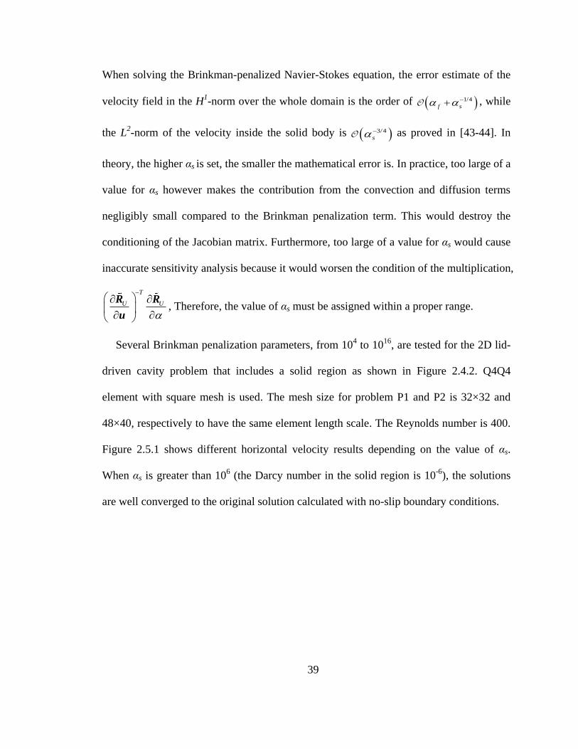
Figure 2.5.2. [P2] Convergence histories according to αs (ReL=400, SUPG+PSPG) ...... 40

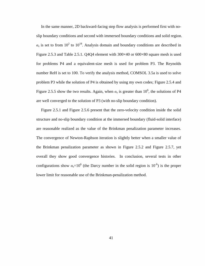
Figure 2.5.3. 2D backward-facing step flow [P3] with no-slip boundary conditions [P4]

with solid solid structure and immersed boundaries ......................................................... 42

Figure 2.5.4. [P4] Horizontal velocity results of P3 and P4 (αs=106) ............................... 43

Figure 2.5.5. [P4] Horizontal velocity at (a) x=2.5, (b) x=4.5 with various αs (ReL=100,

SUPG+PSPG) ................................................................................................................... 43

viii

Figure 2.5.6. [P4] Horizontal velocity oscillation various αs (ReL=100, SUPG+PSPG) (a)

global velocity (b) local view at fluid-solid interface ....................................................... 44

Figure 2.5.7. [P4] Convergence history according to different Brinkman penalization

parameters ......................................................................................................................... 44

Figure 2.5.8. [P5] 2D flow problem around oval obstacle (a) design domain and bcs (b)

analysis setup .................................................................................................................... 46

Figure 2.5.9. [P5] Horizontal velocity results (section A-A′) accoring to the value of

Brinkman penalization parameter (a) global velcoity (b) local velocity view .................. 47

Figure 2.5.10. [P5] Horizontal velocity results (section A-A′) accoring to different mesh

sizes (a) global velcoity (b) local velocity view ............................................................... 47

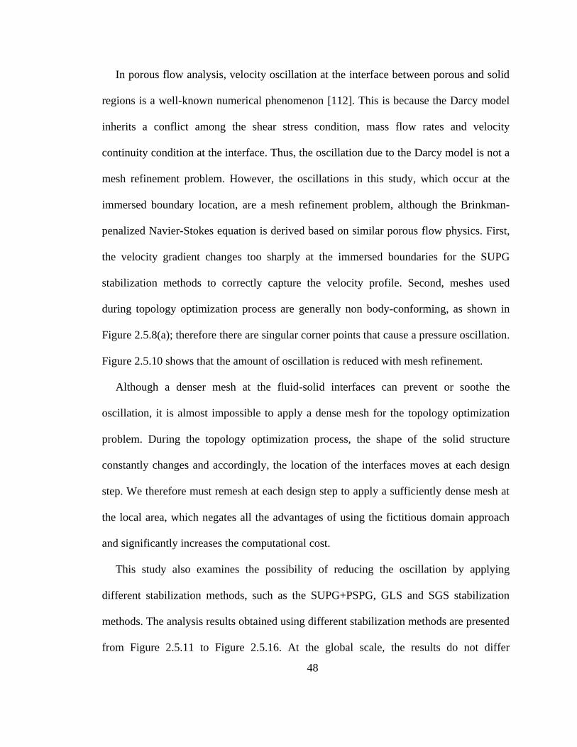
Figure 2.5.11. [P2] Horizontal velocity at section A-A′ with αs=104, ReL=400 using

different stabilization methods (a) global velocity (b) local view .................................... 50





Figure 2.5.14. [P2] Horizontal velocity at section A-A′ with αs=1010

, ReL=400 using


Figure 2.5.15. [P4] Horizontal velocity oscillation according to stabilization methods (a)

global velocity (b) local velocity view at fluid-solid interface ......................................... 52

Figure 2.5.16. [P5] Horizontal velocity results (section A-A′) accoring to different

stabilization methods (a) global velcoity (b) local velocity view ..................................... 52

Figure 3.3.1 [P6] 2D design example (a) design domain and boundary conditions (b)

analysis setup (c) optimization setup ................................................................................ 65

Figure 3.3.2 [P6] Design sensitivity result: (a) finite difference sensitivity (b) adjoint

sensitivity .......................................................................................................................... 66

Figure 3.3.3 [P6] Design process, ReH=0.001 (a) initial design (b) 5st step (c) 10

th step (d)

50th

step ............................................................................................................................. 68

Figure 3.3.4 [P6] Optimization result, ReH=0.001 ........................................................... 68

Figure 3.3.5 [P6] Convergence history, ReH=0.001 ........................................................ 69

Figure 3.3.6 [P6] Design convergence history, ReH=0.001 ............................................. 69

ix

Figure 3.3.7 [P6] Design process, ReH=100 (a) initial design (b) 1st step (c) 10

th step (d)

18th

step (e) 19th

step (f) 20th

step (g) 25th

step (h) 30th

step ............................................. 71

Figure 3.3.8 [P6] Convergence histories, ReH=100 ......................................................... 72

Figure 3.3.9 [P6] Design convergence history, ReH=100 ................................................ 72

Figure 3.3.10 [P6] Design sensitivity results at 18th

step, ReH=100 (a) adjoint sensitivity

(b) finite difference sensitivity .......................................................................................... 73

Figure 3.3.11 [P6] Local sensitivity result and design history, ReH=100 (a) 18th

design

(b) 18th

sensitivity (c) 19th

design ..................................................................................... 74

Figure 3.3.12 [P6] Local design and pressure oscillations, ReH=100 (a) 18th

design (b)

pressure oscillation at section A-A′ (c) back pressure gradients at section B-B′ .............. 75

Figure 3.3.13 Sensitivity oscillations at (a) section A-A′ (b) section B-B′ (c) section C-C′

........................................................................................................................................... 76

Figure 3.3.14 Design history with the densitivy filter (a) 20th

step (b) 43rd

step (c) 44th

step (d) 45th

step ............................................................................................................... 80

Figure 3.3.15 Design history with the sensitivity filter (a) 19th

step (b) 20th

step (c) 21st

step (d) 22nd

step ............................................................................................................... 80

Figure 3.3.16 [P6] Design convergence histories with filters, ReH=100 (a) the density

filter, (b) the sensitivity filter ............................................................................................ 81

Figure 3.3.17 Objective convergence histories according to filtering schemes ............... 82

Figure 3.3.18 [P6] Design history without move-limit, ReH=100 (a) initial design (b) 1st

step (c) 2nd

step (d) 149th

step ........................................................................................... 84

Figure 3.3.19 [P6] Design history with 5% move-limit, ReH=100 (a) initial design (b)

1st step (c) 2

nd step (d) 31

st step ......................................................................................... 84

Figure 3.3.20 [P6] Objective convergence histories according to move-limit, ReH=100 85

Figure 3.3.21 [P6] Design convergence history with 5% move limit, ReH=100 ............. 85



Figure 3.4.2 [P7] Design results minimizing kinetic energy dissipation with GLS

stabilization method a) ReH=10 b) ReH=100 c) ReH=1000 ............................................ 88

x

Figure 3.4.3 [P7] Design results minimizing kinetic energy dissipation at ReH=1000 with

a) GLS stabilization method b) SUPG+PSPG stabilization method c) SGS stabilization

method............................................................................................................................... 89

Figure 3.4.4 [P7] Design result and velotiy profiles at ReH=1000 (a) design result (b)

global velocity at section A-A' (c) local velocity view ..................................................... 91



Figure 3.4.6 [P8] Optimization results: (a) design result, (b) stream line graph .............. 94

Figure 3.4.7 [P8] Convergence histories ........................................................................... 94

Figure 4.3.1. [P9] 2D cooling channel design (a) design domain and boundary conditions

(b) analysis setup (c) optimization setup ........................................................................ 106

Figure 4.3.2. [P9] Design result of 2D cooling channel problems (a) design domain (b)

cooling channel design, ReH=10 (c) streamline graph, ReH=10 (d) cooling channel

design, ReH=100 (e) streamline graph, ReH=100 .......................................................... 109

Figure 4.3.3. [P9] Design and temperature results of 2D cooling channel problems at

Reh=100 (a) design domain (b) design result (c) correct temperature profile (d) calculated

temperature profile with solid-penetrating flow motion ................................................. 110

Figure 4.3.4. [P9] Case 1: design and temperature results (a) design (b) temperature ... 112

Figure 4.3.5. [P9] Case 2: design and temperature results (a) design (b) correct

temperature (c) calculated temperature profile with solid-penetrating flow motion ...... 112

Figure 4.3.6. [P10] Modified design domain of P9 and the design result (a) modified

design domain (b) design result and streamline graph at ReH=10 (c) design result and

streamline graph at ReH=100 ......................................................................................... 114

Figure 4.3.7. [P11] Modified analysis domain of P9 with bypass line ........................... 115

Figure 4.3.8. [P9] Design result and pressure profile of the 2D cooling channel problem

......................................................................................................................................... 116

Figure 4.3.9. [P9] Design result of 2D cooling channel problems with new multi-

objective function, Reh=100 (a) design result (b) temperature profile ........................... 117

Figure 4.3.10. [P9] Pressure drop results according to the objective function ............... 117

Figure 4.4.1. [P9] 2D design result with antifreeze (50%) flow (a) design domain (b)

ReH=10, Pr=7.2 (c) ReH=100, Pr=7.2 (d) ReH=1000, Pr=7.2 ...................................... 121

xi

Figure 4.4.2. [P9] 2D design result with air flow (a) design domain (b) ReH=10, Pr=0.72

(c) ReH=100, Pr=0.72 (d) ReH=1000, Pr=0.72 .............................................................. 122

Figure 4.4.3. [P12] 3D cooling channel design (a) design domain and boundary

conditions (b) analysis setup (c) optimization setup ....................................................... 124

Figure 4.4.4. [P12] 2D design result with air flow (a) design domain (b) ReH=10,

Pr=0.72 (c) ReH=100, Pr=0.72 (d) ReH=1000, Pr=0.72 ............................................. 126


Pr=0.72 (c) ReH=100, Pr=0.72 (d) ReH=1000, Pr=0.72 ............................................. 127

Figure 5.2.1. Crack growth in the engine head [8] ......................................................... 134

xii

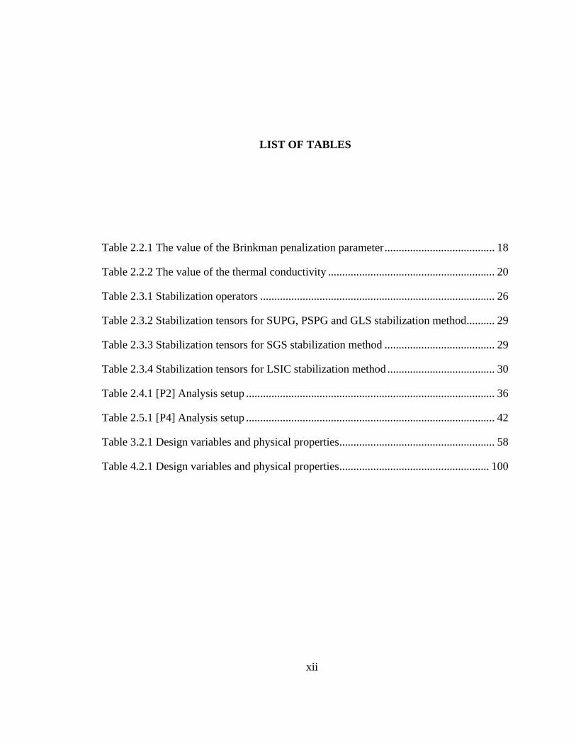
LIST OF TABLES

Table 2.2.1 The value of the Brinkman penalization parameter ....................................... 18

Table 2.2.2 The value of the thermal conductivity ........................................................... 20

Table 2.3.1 Stabilization operators ................................................................................... 26

Table 2.3.2 Stabilization tensors for SUPG, PSPG and GLS stabilization method.......... 29

Table 2.3.3 Stabilization tensors for SGS stabilization method ....................................... 29

Table 2.3.4 Stabilization tensors for LSIC stabilization method ...................................... 30

Table 2.4.1 [P2] Analysis setup ........................................................................................ 36

Table 2.5.1 [P4] Analysis setup ........................................................................................ 42

Table 3.2.1 Design variables and physical properties ....................................................... 58

Table 4.2.1 Design variables and physical properties ..................................................... 100

xiii

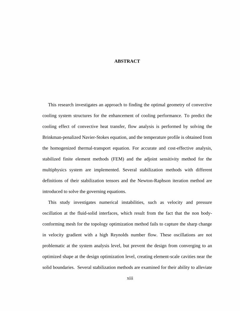
ABSTRACT

This research investigates an approach to finding the optimal geometry of convective

cooling system structures for the enhancement of cooling performance. To predict the

cooling effect of convective heat transfer, flow analysis is performed by solving the

Brinkman-penalized Navier-Stokes equation, and the temperature profile is obtained from

the homogenized thermal-transport equation. For accurate and cost-effective analysis,

stabilized finite element methods (FEM) and the adjoint sensitivity method for the

multiphysics system are implemented. Several stabilization methods with different

definitions of their stabilization tensors and the Newton-Raphson iteration method are

introduced to solve the governing equations.

This study investigates numerical instabilities, such as velocity and pressure

oscillation at the fluid-solid interfaces, which result from the fact that the non body-

conforming mesh for the topology optimization method fails to capture the sharp change

in velocity gradient with a high Reynolds number flow. These oscillations are not

problematic at the system analysis level, but prevent the design from converging to an

optimized shape at the design optimization level, creating element-scale cavities near the

solid boundaries. Several stabilization methods are examined for their ability to alleviate

xiv

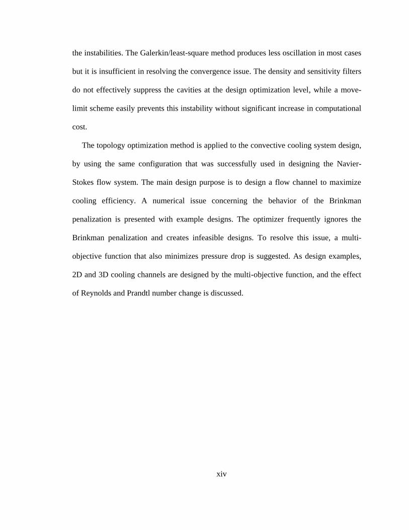
the instabilities. The Galerkin/least-square method produces less oscillation in most cases

but it is insufficient in resolving the convergence issue. The density and sensitivity filters

do not effectively suppress the cavities at the design optimization level, while a move-

limit scheme easily prevents this instability without significant increase in computational

cost.

The topology optimization method is applied to the convective cooling system design,

by using the same configuration that was successfully used in designing the Navier-

Stokes flow system. The main design purpose is to design a flow channel to maximize

cooling efficiency. A numerical issue concerning the behavior of the Brinkman

penalization is presented with example designs. The optimizer frequently ignores the

Brinkman penalization and creates infeasible designs. To resolve this issue, a multi-

objective function that also minimizes pressure drop is suggested. As design examples,

2D and 3D cooling channels are designed by the multi-objective function, and the effect

of Reynolds and Prandtl number change is discussed.

1

CHAPTER 1

1. INTRODUCTION

1.1. Motivation and goal

Design of an improved cooing system has become a more critical task for developing

new products. In the automotive industry, next-generation engines, motors, generators

and converters are designed more compactly for reducing mass, minimizing required

space, reducing frictional loss and increasing fuel efficiency. Electric circuits also

become denser and faster and multiprocessor computer system chips are clustered in

closer proximity. This compactness makes power density of equipment higher and causes

thermal load to constantly increase. As a consequence, the ability to efficiently remove

heat from an increasingly restricted space is currently a very critical issue. The need to

develop optimization methodologies in order to design efficient cooling systems is

drawing the attention of a large number of industrial and university researchers.

Sizing, shape and topology optimization methods have great potential to advance

cooling structure design. The rapid growth of computational power and CAE software

makes it possible to model complex geometries and accurately take into account physical

2

processes and material behavior with reasonable computational efforts. Still, the

developing procedure of cooling structure depends on the traditional trial-and-error

method, which is very time consuming and requires enormous experimental data.

Moreover, the trial and error method may become problematic because the outcome

depends mainly on the expertise of the designer, and there is no guarantee of design

improvement during the design process. Hence, there is a need to develop automated and

computerized design optimization approaches, such as sizing, shape and topology

optimization, which automatically determine a design change and furthermore guarantee

the improvement of the structure design. These automated optimization processes speed

up the design process and reduce development cost.

In this work, design optimization of convective cooling systems is carried out using

the topology optimization approach. Of the automated optimization methods, topology

optimization was most recently introduced by Bensøe and Kikuchi [1], and it has been

successfully applied to structural design optimization problems. The main advantages of

topology optimization are first, that it allows change of the structural topology during the

optimization process and, second, that the final design barely depends on the initial

design. Since the structural topology determines the configuration of cooling channels,

the choice of appropriate structural topology is usually the most decisive factor

influencing the efficiency of a new design. However, by using the size and shape

optimization methods, it is challenging to change the roughly guessed structural topology

in the conceptual stage of the optimization process. Therefore, the topology optimization

method is a very valuable tool, particularly in the beginning stages, in that it can optimize

the structural topology.

3

This new optimization approach has been applied to various physics problems such as

electromagnetics, heat conduction, and fluidics. Yet, the topology optimization approach

for heat convection problems is still in the initial stage, and has not been well established.

Previous topology optimization problems for heat transfer problems focused mainly on

heat conduction, although the heat convection coefficient ‘h’ is sometimes applied. In this

study, fluid analysis is also carried out for topology optimization to produce better

optimization results focusing on the behavior of coolant flow. For this purpose, this study

first extends the study of topology optimization in two steps. First, it applies the topology

optimization method of linear Stokes flow systems for designing nonlinear Navier-Stokes

flow systems. Then, it combines the results with previous topology optimization studies

of heat transfer problems.

Since topology optimization generally requires high computational cost, it is essential

to establish a cost-effective procedure for system analysis and design optimization. This

study presents the adjoint sensitivity method for nonlinear, weakly-coupled multiphysics

systems and introduces stabilized finite element methods to reduce the computational

cost without serious loss of accuracy. The stabilization method is also essential to

simulate convective-dominant problems such as high Reynolds flow problems. Finally,

this dissertation discusses numerical issues that arise when the previous topology

optimization approach is applied to nonlinear and multiphysics systems.

In the introduction, the literature on cooling system design is summarized. In addition,

the literature on the topology optimization and stabilized finite element methods are

described. Then, the outline of this dissertation is presented.

4

1.2. Cooling system design optimization

Cooling system design is an important element in many industrial applications, such

as cooling flows in combustion engines, electric motors and battery packs. In automotive

industries, battery thermal management is critical in achieving performance and in

extending the life of batteries in electric and hybrid vehicles under real driving conditions

[2]. Many studies have sought to develop accurate finite element models to predict the

temperature distribution in battery cells and to improve thermal performance [3-4]. In any

engine part, the cooling system must remove enough heat to allow proper engine function

and evenly distribute the heat, primarily throughout the water jacket. Improper design of

the cooling flow path can result in significant overheating of engine parts, which limits

performance and durability, and causes structural damage. On the other hand, an

optimized engine cooling system leads to improved durability and lower fuel

consumption [5]. For this reason, optimization methodologies for better engine coolant

flow [6-7] and engine gasket hole designs [5, 8-9] have been developed.

Also, the growth in power electronics technologies has produced smaller devices with

increased levels of current and voltage. As the power density of these devices becomes

greater, thermal loss is increased, which leads to an increase in component failure and a

decrease in reliability. Therefore, designers attempt to improve thermal management

through innovation of cooling system design. First, thermal analysis was performed,

providing guidelines for designing cooling channels and heat sinks for motors and

converters [10-11]. Khorunzhii et al. [12] investigated the micro cooling design of a pin-

fin heat converter for a power semiconductor.

5

Then, the above-mentioned optimization processes are all performed by manually and

intuitively modifying design parameters. However, this process does not guarantee design

improvement during the design process. To achieve design automation, many algorithms

for numerical optimization technologies have been proposed such as size optimization,

parametric shape optimization, shape optimization and topology optimization. The main

advantage of these methods is that a design change will be determined automatically and

the improvement of the structure is mathematically guaranteed.

For example, size optimization processes were used for pin-fin heat sink designs [13-

15] to determine the best uniform fin heights, non-uniform fin heights and non-uniform

fin gaps respectively. Figure 1.2.1 shows the optimized results of heat sink design using

size optimization. Also, a parametric shape optimization technique was used to design a

better cooling system. Lee et al. [16] selected geometric parameters to define overall

design structure such as channel width, length, height, pin pitch and angles (see Figure

1.2.2) and found the best values for these parameters. Similarly, this technique is used in

designing heat sink shape [17-19] and dimple shape in the cooling channel for laminar

flow and turbulent flow, in [20-21] respectively. Also, Kuhl et al. presented optimization

processes for designing cooling channels in the combustion chamber of a rocket engine

[22].

6

Figure 1.2.1. Schematic diagram of different heights design results for pin-fin heat sink

[14]

Figure 1.2.2. Schematic diagram of design variables in parametric shape optimization [16]

7

While parametric shape optimization uses geometric parameters, shape optimization

uses geometrical information of boundary mesh. To optimize structure, shape

optimization searches for the best location of boundary by shape variations of the mesh

morphing. Balagangadhar et al. [23] shows the sensitivity calculation for thermal fluid

shape optimization. Two dimensional oval tubes in the heat exchangers are optimized for

maximizing heat transfer [24-25] and three dimensional corrugated wall cooling channel

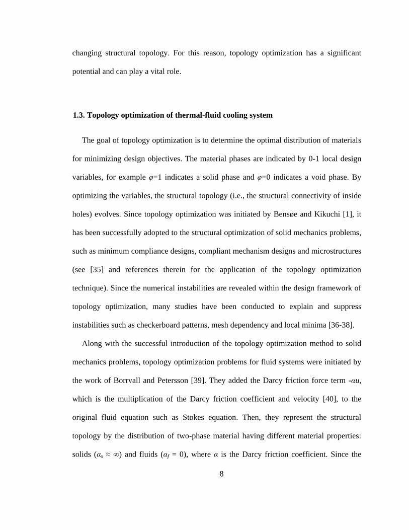
[26]. Airfoil-type heat exchangers are designed [27-28] as shown in Figure 1.2.3.

Recently, Non-Uniform, Rational, B-spline (NURB) is widely used for shape

optimization which enables easy control of boundary geometry. NURB is used to design

heat sink [29-30] and internally finned cooling pipe [31-33].

Figure 1.2.3. Shape deformation by shape optimization process (left: initial, right:

deformed) [34]

However, size and shape optimization have a limitation when they handle complicated

geometry and topology such as engine cooling jacket. For example, shape and location of

holes sometimes play a vital role in cooling system as shown in engine gasket design [5-

9]. It is impractical to use size and shape optimization for designing new holes by

8

changing structural topology. For this reason, topology optimization has a significant

potential and can play a vital role.

1.3. Topology optimization of thermal-fluid cooling system

The goal of topology optimization is to determine the optimal distribution of materials

for minimizing design objectives. The material phases are indicated by 0-1 local design

variables, for example φ=1 indicates a solid phase and φ=0 indicates a void phase. By

optimizing the variables, the structural topology (i.e., the structural connectivity of inside

holes) evolves. Since topology optimization was initiated by Bensøe and Kikuchi [1], it

has been successfully adopted to the structural optimization of solid mechanics problems,

such as minimum compliance designs, compliant mechanism designs and microstructures

(see [35] and references therein for the application of the topology optimization

technique). Since the numerical instabilities are revealed within the design framework of

topology optimization, many studies have been conducted to explain and suppress

instabilities such as checkerboard patterns, mesh dependency and local minima [36-38].

Along with the successful introduction of the topology optimization method to solid

mechanics problems, topology optimization problems for fluid systems were initiated by

the work of Borrvall and Petersson [39]. They added the Darcy friction force term -αu,

which is the multiplication of the Darcy friction coefficient and velocity [40], to the

original fluid equation such as Stokes equation. Then, they represent the structural

topology by the distribution of two-phase material having different material properties:

solids (αs ≈ ∞) and fluids (αf = 0), where α is the Darcy friction coefficient. Since the

9

Darcy friction coefficient has infinite value in the solid region, the velocity in the solid

region converges to zero, satisfying no-slip boundary conditions. On the other hand, the

added Darcy friction term becomes zero in the fluid region Ωf, and the original fluid

equation is recovered. It should be noted that this analysis method is a fictitious domain

approach with Brinkman penalization based on porous media theory, and the

mathematical justification is achieved in [41-44]. To combine this analysis approach with

the conventional topology optimization technique, the Darcy friction coefficient (the

Brinkman penalization parameter) α is interpolated as a function of local design variables

φ. With this interpolation, φ=0 indicates a fluid region (i.e., α(0)=0) and φ=1 indicates a

solid region (i.e., α(1) ≈ ∞) so that the design problem become a typical 0-1 topology

optimization problem.

Following this idea, numerous studies have been performed. Wiker et al. added

effective viscosity variation as an additional property control of two-phase material [45-

46]. Gersborg-Hansen et al. suggested a topology optimization method for Navier-Stokes

flow [47], which is similar to the Borrvall and Petersson’s work [39]. Various example

problems followed such as Stokes flow [48], microfluidics [49-50], 3D Stokes flow [51],

mixing [52-53], reactor design [54] and fluid-structure interaction problem [55]. In

addition, Pingen et al. presented topology optimization for nano-fluid problem by using

Lattice Boltzmann equation [56-57] and Duan et al. demonstrated topology optimization

for Stokes’ flow and Navier-Stokes’ flow via variational level set method [58-60]. In

industrial applications, Daimler-Chrysler and Volkswagen engineers demonstrated the

possibility of topology optimization for air channel flow design [61-62].

10

Besides the successful utilization of topology optimization for fluid systems, heat

transfer problems have also been an issue of great concern as applications of the topology

optimization method. Topology optimization is first applied to pure heat conduction

problems [63-67]. In addition to heat conduction, heat convection physics is also taken

into consideration by employing convection the coefficient ‘h’ in [68-72]. In

conventional topology optimization methods, it is not easy to clearly define boundary

locations in the middle of the process, since they are blurry and constantly changing.

Therefore, previous research assumed that the heat convection coefficient was constant

without considering fluid motion, which varies significantly according to the geometry.

Subsequently, these approaches may be infeasible for designing cooling channels that

prevent re-circulation areas and hot spots.

To overcome this issue, Iga et al. [73] recently applied the design-dependent topology

optimization method developed by Chen and Kikuchi [74]. They approximated design

dependent heat convection coefficient by using the flow simulation of a simplified

periodic fin model. Yet, the possibility of practical implementation of their assumption is

an open question. Therefore, this study performs flow motion analysis without using such

simplified model so as to figure out accurate heat transfer condition at the fluid-solid

interfaces. Successful integration of CFD analysis into the topology optimization method

of heat transfer problems might be a good solution, which has significant potential for the

future design of complex cooling system.

11

1.4. Stabilized finite element method

Stabilized finite element methods are now commonly used in finite element

computation of flow problems due to the computational difficulties and shortcomings of

the Galerkin finite element method (GFEM) [75-76]. The main issue for the standard

GFEM is the occurrence of velocity wiggles in flow problems. This numerical instability

is a node-to-node oscillation, producing a large velocity gradient caused by the inability

of GFEM to capture the steep gradient. It results in an imbalance between the convective

and diffusive terms in the equation. Stabilized finite element methods bring numerical

stability to flow problems with high Reynolds numbers and coarse meshes, without

introducing excessive numerical dissipation. They also bring numerical stability to

incompressible flow computation when using equal-order interpolation functions for

velocity and pressure, which significantly reduce the computational cost.

Some of the earliest stabilized formulations are the streamline-upwind/Petrov–

Galerkin (SUPG) formulation [77-78] and the pressure-stabilizing/Petrov–Galerkin

(PSPG) formulation [79-80]. The SUPG method addresses the wiggle problem by

introducing the concept of adding diffusion along the streamlines. The PSPG method

allows us to use equal-order interpolation functions for velocity and pressure, without

considering the LBB stability condition. Another method for enhancing the stability of

the GFEM for incompressible flow is the Galerkin/Least-squares (GLS) approach, which

involves the addition of various least-squares terms to the original Galerkin variational

statement. Development and popularization of the GLS methods for flow problems [79,

81-84] follows as a generalization of SUPG and PSPG methods. The underlying

12

philosophy of the SUPG and GLS methods is to strengthen the classical variational

formulations so that the discrete approximations, which would otherwise be unstable,

become stable and convergent.

The sub-grid scale (SGS) stabilization method originated from the concept of

representing multiscale phenomenon, which delivers similar results to the SUPG and

GLS techniques unless the reaction term is dominant. Also, the variational multiscale

method (VMS) was introduced by Hughes [85], providing the necessary mathematical

framework for the SGS models. In this method, the different stabilization techniques

come together as special cases of the underlying sub-grid scale concept. It should be

noted that some of the stabilized methods discussed above were somewhat ad hoc in

nature [75-76]. However, the introduction and development of the VMS method has

remedied much of the confusion regarding stabilized procedures and provided much

needed explanation and consistency in implementation. Masud and co-workers developed

VMS formulations for the Darcy-Stokes flow equations [86-87], the advection–diffusion

equation [88], the convection-diffusion-reaction equations [89] and the incompressible

Navier–Stokes equations [90].

In these stabilization methods, an embedded stabilization tensor most commonly

known as τ plays an important role. The definitions of the stabilization tensors have been

extensively studied and developed for the SUPG, PSPG and GLS stabilization methods

[77, 84, 91-96] as well as for the SGS stabilization method [97-98]. The stabilization

tensors are expressed in terms of the ratios of the norms of the matrices or vectors, taking

into account local length scales, the advection field and the element Reynolds number.

13

1.5. Outline of dissertation

The remainder of this dissertation is organized as follows:

Chapter 2 presents an analysis method for topology optimization of thermal-fluid

systems. Numerical issues in system analysis are described. Chapter 3 presents the

topology optimization of Navier-Stokes flow systems and investigated numerical

instabilities of the topology optimization of these nonlinear systems. Chapter 4 presents

the topology optimization of thermal-fluid systems. After numerical issues concerning

these multiphysics problems are investigated, 2D and 3D convective cooling systems are

designed. Chapter 5 concludes the dissertation with remarks and future works.

Appendices include the detailed derivations of the multi-scale stabilization tensors.

14

CHAPTER 2

2. THERMAL-FLUID ANALYSIS FOR TOPOLOGY OPTIMIZATION

2.1. Introduction

This chapter presents an analysis method for topology optimization of thermal-fluid

systems. A fictitious domain approach [42-44, 99], with immersed boundaries and

Brinkman penalization, which is based on the porous fluid theory, has been mainly used

for the topology optimization of linear Stokes flow systems [45-46, 51, 100-102]. This

study extends the analysis approach to topology optimization of nonlinear Navier-Stokes

flow systems and further multiphysics thermal-fluid systems.

To establish a stable and cost-effective method, various stabilized finite element

methods, such as SUPG, PSPG, GLS, SGS and VMS, are tested and compared with

different stabilization tensors. The obtained solutions of the Brinkman-Penalized Navier-

Stokes equation, which is based on the fictitious domain approach [42-44, 99], are

confirmed whether or not the no-slip boundary condition at the immersed solid

boundaries and the zero-velocity condition in the solid regions are satisfied. Numerical

15

issues concerning the value of the Brinkman penalization parameter are studied, and

numerical instability at the immersed boundaries is investigated.

The outline of Chapter 2 is as follows: Section 2.2 introduces a system analysis

method for thermal-fluid systems; Brinkman-penalized Navier-Stokes equation and

homogenized thermal transport equation are explained. Section 2.3 presents different

stabilized finite element methods and stabilization tensors. Section 2.4 explains in detail

how to implement the Newton-Raphson methods. Section 2.5 discusses numerical issues

arise from the solutions of Brinkman-penalized Navier-Stokes equation. Section 2.6

summaries this section.

2.2. Governing equations for topology optimization

During the topology optimization process for convective cooling systems, design

domains consists of fluid, solid and porous regions, as shown in Figure 2.2.1. To simulate

fluid flows around porous and solid obstacles having complex geometries, various

immersed boundary methods can be used. The main advantage of using immersed

boundary methods is efficient implementation of fixed non-body conformal Cartesian

grids for representing complex stationary or moving solid boundaries. The shapes of solid

structures are continuously changed during the topology optimization process. Therefore,

it is more efficient to use the same fixed Cartesian grid than body-conformal grids that

usually needs to be re-generated at each optimization step.

16

Figure 2.2.1. Fluid-solid system in topology optimization for fluid systems

Figure 2.2.2. Representation of the solid region as a porous medium [42]

17

2.2.1. Brinkman-penalized Navier-Stokes equation

Among immersed boundary methods, the Brinkman penalization method [42-44, 99],

which is proposed for solving incompressible viscous flow by penalizing the momentum

equation, is widely used for the topology optimization of Stokes flow systems. The main

idea of this method is to model solid obstacles as porous media with porosity near unity,

but permeability approaching zero as shown in Figure 2.2.2.

A steady-state incompressible fluid is governed by the Navier-Stokes equation with

the Boussinesq approximation as:

2

f f p v v v = f (2.2.1)

0v = . (2.2.2)

Here, ρf is fluid density, μf fluid dynamic viscosity, v fluid velocity, p pressure and f is

body force. I assume incompressible flow, and gravitational acceleration and buoyancy

force are not taken into consideration from a practical standpoint.

Then, the effect of the no-slip boundary condition is implemented by adding the

Brinkman penalization term αv, which is physically interpreted as the Darcy-friction

force, to the Navier-Stokes equation as

2

f f p v v v v = f (2.2.3)

18

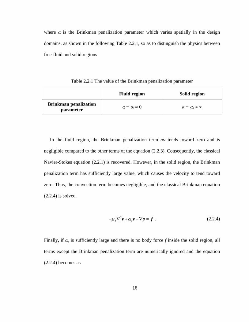
where α is the Brinkman penalization parameter which varies spatially in the design

domains, as shown in the following Table 2.2.1, so as to distinguish the physics between

free-fluid and solid regions.

Table 2.2.1 The value of the Brinkman penalization parameter

Fluid region Solid region

Brinkman penalization

parameter α = αf ≈ 0 α = αs ≈ ∞

In the fluid region, the Brinkman penalization term αv tends toward zero and is

negligible compared to the other terms of the equation (2.2.3). Consequently, the classical

Navier-Stokes equation (2.2.1) is recovered. However, in the solid region, the Brinkman

penalization term has sufficiently large value, which causes the velocity to tend toward

zero. Thus, the convection term becomes negligible, and the classical Brinkman equation

(2.2.4) is solved.

2

f s p v v = f . (2.2.4)

Finally, if αs is sufficiently large and there is no body force f inside the solid region, all

terms except the Brinkman penalization term are numerically ignored and the equation

(2.2.4) becomes as

19

0s v = , (2.2.5)

which forces the velocity to converge to zero.

Since the velocity converges to zero in the solid region, the no-slip boundary condition

at the solid surface is automatically satisfied, and there is no need to explicitly specify the

fluid-solid interface condition. Likewise, the fluid velocity inside solid structures

converges to zero, thus physically correct flow motions near solid obstacles are obtained.

Mathematical justification of this method, based on the L2-penalized equation, is derived

in [43-44].

I set the value of αf to zero without any numerical difficulties, but the value of penalty

parameter αs should be carefully assigned. The error estimate of the velocity field in the

H1-norm over the whole domain is the order of 1/4

f s O , whereas the L2-norm of

the velocity error inside the solid body is 3/4

sO . In theory, the higher αs is set, the

smaller the mathematical error is. However, in practice, using too large αs decreases both

the convergence speed and accuracy of Newton-Raphson iteration method when solving

the nonlinear equation. Thus, the value of penalty parameter αs should be carefully pre-

assigned to reduce both theoretical errors and numerical errors, which will be presented

in section 2.5.1.

2.2.2. Homogenized thermal transport equation

The traditional thermal transport equation is expressed as

20

0f pC T k T v . (2.2.6)

where T is temperature, Cp constant-pressure specific heat and k is thermal conductivity.

The viscous dissipation term is ignored compared to other terms from a practical

standpoint [103-105]. In this work, the thermal conductivity varies in the two different

regions as shown in Table 2.2.2.

Table 2.2.2 The value of the thermal conductivity


Thermal conductivity k = kf k = ks

In the solid region, the fluid velocity v becomes zero due to the Brinkman

penalization, so that the thermal transport equation (2.2.6) becomes a pure conduction

equation without the leftmost convective term as

0sk T . (2.2.7)

In the fluid region, the energy equation (2.2.6) maintains the original form with the

thermal conductivity of fluid as

0f p fC T k T v (2.2.8)

21

These governing equations, for fluid physics (2.2.3) and heat transfer physics (2.2.6),

are weakly coupled only through fluid velocity because all material properties are

assumed to be independent from temperature and buoyancy force is ignored from a

practical standpoint. Therefore, the momentum equation (2.2.3) and the incompressibility

constraint (2.2.2) can first be solved together without considering temperature profile.

Then the temperature profile is obtained by solving the energy equation (2.2.6). This two-

step analysis strategy after decoupling temperature significantly decreases computational

cost.

2.2.3. Slightly compressible fluid condition

Instead of the incompressible constraint (2.2.2), Anton Evgrafov suggested solving a

slightly compressible fluid model so as to deal with impenetrable inner walls that may

appear in the flow domain and to obtain a closed design-to-flow mapping [106]. This

slightly compressible condition is implemented with a penalization in the continuity

equation as

1

p

v = . (2.2.9)

where λ is a penalty parameter, which ensures the continuity equation when it has a

sufficiently large value. In theory, this is a mathematically good approach. However, in

22

practice, there exist numerical difficulties in applying this slightly compressible condition

for the topology optimization of Navier-Stokes flow systems.

First of all, too large of a value for λ decreases the effect of the Brinkman penalization

inside solid regions preventing the velocity inside solid regions from converging to zero,

whereas too small of a value for λ produces an inaccurate solution in the fluid analysis.

By implementing the equation (2.2.9), the momentum equation including the Brinkman

penalization term will become as

f f v v ε v v v = f (2.2.10)

where T

ε v = v + v . Since this momentum equation has two penalization terms

v and S v inside the solid region, the two values of λ and αs should be

carefully selected in order to make both penalizations function properly. For example, if

the two values are very similar to each other, the momentum equation in the solid region

will become as

0S v v = . (2.2.11)

This equation does not guarantee the zero velocity condition in the solid region. To

satisfy both the slightly compressible and zero-velocity conditions, the value of αs should

be significantly larger than the value of λ to achieve both penalizations because the

Brinkman penalization (v = 0) automatically satisfies the incompressible constraint.

23

Computational experience indicates that, although these values are dependent on

problems, the value of αs should be greater than 106×λ in some Navier-Stokes flow

problems. Then, according to [75, 107-108], values of λ between 107 and 10

9 are

adequate in most practical situations with double precision 64-bit words, which means αs

should be greater than 1013

. This too large value is hardly appropriate. It impairs both the

convergence speed and accuracy of the Newton-Raphson iteration.

Instead of solving equation (2.2.10), another modified penalty formulation can be

obtained by applying the assumption of a slightly compressible barotropic fluid. The

modified penalty formulation is expressed as an iterative algorithm as follows:

1

11 1

n

T nn

A Q Fu

Q I pp. (2.2.12)

Here, Au is the summation of viscous, convective and Brinkman penalization terms, F

the body force, and Qp and QTu are the pressure gradient and divergence of the velocity

field, respectively. Then, the second set of equations takes the form

1 1n n T n p p Q u . (2.2.13)

This modified formulation is equivalent to the introduction of a false transient in the

steady-state calculation. Furthermore, it allows to use smaller penalty parameters, while

satisfying the incompressibility constraint practically to the round-off error limit [107].

Therefore, using this modified penalty formulation with small λ might resolve the

24

numerical issues concerning too large of a value for αs. However, this research focus on a

nonlinear system, so adding this iterative algorithm to the Newton-Raphson iteration will

significantly increase the computational cost. In conclusion, more studies are needed to

properly applying both the slightly compressible condition and the Brinkman penalization

to highly nonlinear Navier-Stokes flow analyses, and this research therefore limits itself

to incompressible fluids.

2.3. Stabilized finite element method

Stabilized finite element methods are used to solve the weakly coupled governing

equations (2.2.3) and (2.2.6). Stabilized finite element methods are now commonly used

in finite element analysis of flow-concerned problems. They bring numerical stability to

high Reynolds number flow problems without creating excessive numerical dissipation.

They also bring numerical stability to incompressible flow computations when using

equal-order interpolation functions for velocity and pressure [75-76, 80, 109]. The equal-

order linear interpolation significantly reduces computational cost, thus it is very practical

for the topology optimization that generally requires high computational power.

Moreover, the equal-order linear interpolation leads to the convenient implementation of

the analysis, and accordingly makes it simple to derive the design sensitivity.

The nonlinear Brinkman-penalized Navier-Stokes equation and the homogenized

thermal transport equation can be assumed as a convection-diffusion-reaction equation

with or without a zero reaction term. Therefore, we can define the two governing

equations as

25

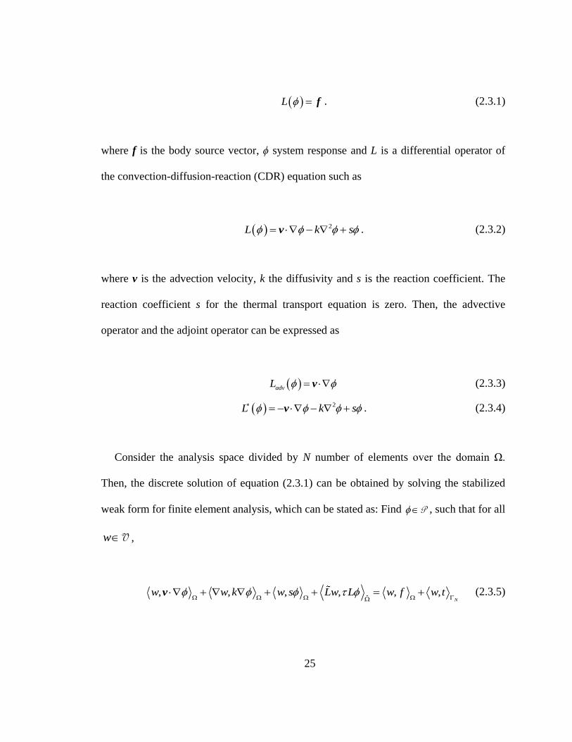
L f . (2.3.1)

where f is the body source vector, ϕ system response and L is a differential operator of

the convection-diffusion-reaction (CDR) equation such as

2L k s v . (2.3.2)

where v is the advection velocity, k the diffusivity and s is the reaction coefficient. The

reaction coefficient s for the thermal transport equation is zero. Then, the advective

operator and the adjoint operator can be expressed as

advL v (2.3.3)

2L k s v . (2.3.4)

Consider the analysis space divided by N number of elements over the domain Ω.

Then, the discrete solution of equation (2.3.1) can be obtained by solving the stabilized

weak form for finite element analysis, which can be stated as: Find P , such that for all

wV ,

, , , , , ,N

w w k w s Lw L w f w t

v (2.3.5)

26

where , d

is the inner product in L2, w an weighting function, L a

stabilization operator applied to the variation in the stabilization term, Ω the spatial

analysis domain, ГN the Neumann boundaries of the domain and is the sum of

element interiors, i.e., 1

N e

i . V and P are the standard variational functional

spaces. For the detailed procedure, the reader is referred to [89].

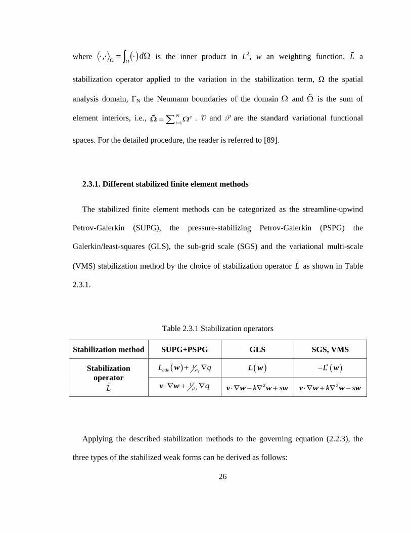
2.3.1. Different stabilized finite element methods

The stabilized finite element methods can be categorized as the streamline-upwind

Petrov-Galerkin (SUPG), the pressure-stabilizing Petrov-Galerkin (PSPG) the

Galerkin/least-squares (GLS), the sub-grid scale (SGS) and the variational multi-scale

(VMS) stabilization method by the choice of stabilization operator L as shown in Table

2.3.1.

Table 2.3.1 Stabilization operators

Stabilization method SUPG+PSPG GLS SGS, VMS

Stabilization

operator

L

1fadvL q w L w

L w

1f

q v w 2k s v w w w 2k s v w w w

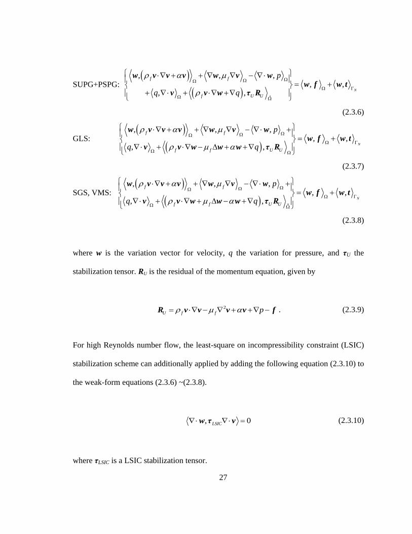
Applying the described stabilization methods to the governing equation (2.2.3), the

three types of the stabilized weak forms can be derived as follows:

27

SUPG+PSPG:

, , ,, ,

, ,N

f f

f U U

p

q q

w v v v w v ww f w t

v v w τ R

(2.3.6)

GLS:

, , ,, ,

, ,N

f f

f f U U

p

q q


v v w w w τ R

(2.3.7)

SGS, VMS:

, , ,, ,

, ,N

f f

f f U U

p

q q


v v w w w τ R

(2.3.8)

where w is the variation vector for velocity, q the variation for pressure, and τU the

stabilization tensor. RU is the residual of the momentum equation, given by

2

U f f p R v v v v f . (2.3.9)

For high Reynolds number flow, the least-square on incompressibility constraint (LSIC)

stabilization scheme can additionally applied by adding the following equation (2.3.10) to

the weak-form equations (2.3.6) ~(2.3.8).

, 0LSIC w τ v (2.3.10)

where τLSIC is a LSIC stabilization tensor.

28

Likewise, by applying the stabilization methods to the thermal transport equation

(2.2.6), the stabilized weak form becomes as follows:

SUPG: , , , ,N

f p f p T Tw C T w k T C T w

v v τ R t

(2.3.11)

GLS: , , , ,N

f p f p T Tw C T w k T C T k T w

v v τ R t

(2.3.12)

SGS, VMS: , , , ,N

f p f p T Tw C T w k T C T k T w

v v τ R t

(2.3.13)

where w is the variation for temperature, and τT is the stabilization tensor RT is the

residual of the energy equation, given by

T f pC T k T R v . (2.3.14)

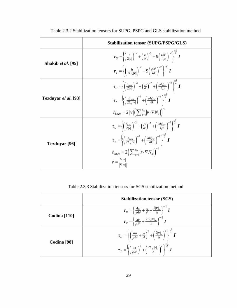
2.3.2. Stabilization tensors

Each stabilization method has a stabilization tensor, such as τU, τLSIC and τT. Several

schemes to determine the stabilization tensors are tested. For SUPG, PSPG and GLS

stabilization methods, the stabilization tensors as suggested in [93, 95-96] are used as

shown in Table 2.3.2. Here, I is an identity matrix, h the length of the finite element and

Na is the shape function associated with node number a. For SGS and LSIC stabilization

methods, the schemes shown in Table 2.3.3 and Table 2.3.4 are used to calculate their

stabilization tensor, respectively.

29

Table 2.3.2 Stabilization tensors for SUPG, PSPG and GLS stabilization method

Stabilization tensor (SUPG/PSPG/GLS)

Shakib et al. [95]

2

2

22 2

2 2

12

12

2 4

2 4

9

9p

U

T

hh

hhC k

v

v

τ I

τ I

Tezduyar el al. [93]

2

2

22 2

2 2

1

1

12

12

2 4

2 4

2

UGN UGN

UGN UGN

p

en

U

T

n

UGN aa

h h

h h

C k

h N

v

v

τ I

τ I

v v

Tezduyar [96]

2

2

22 2

2 2

1

1

12

12

2 4

2 4

2

RGN RGN

RGN RGN

p

en

U

T

n

RGN aa

h h

h h

C k

h N

v

v

v

v

τ I

τ I

r

r

Table 2.3.3 Stabilization tensors for SGS stabilization method

Stabilization tensor (SGS)

Codina [110]

2

2

124

124 p

U

T

hh

Ckhh

v

v

τ I

τ I

Codina [98]

2

2

22

22

12

12

24

24 p

U

T

hh

Ckhh

v

v

τ I

τ I

30

Table 2.3.4 Stabilization tensors for LSIC stabilization method

Stabilization tensor

Tezduyar el al. [93]

1

1

2

2

2

Re

Re / 3 Re 3

1 Re 3

en

LSIC

n

UGN aa

UGN

UGN UGN

UGN

UGN

UGN

h

h

z

h N

z

v

v

v v

Tezduyar [96]

2

2

22 2

1

1

12

2 4

(1,1)

2 ,

RGN RGN

en

LSIC U

U

n

RGN aa

h h

h N

v

v

v

τ v

τ I

r r

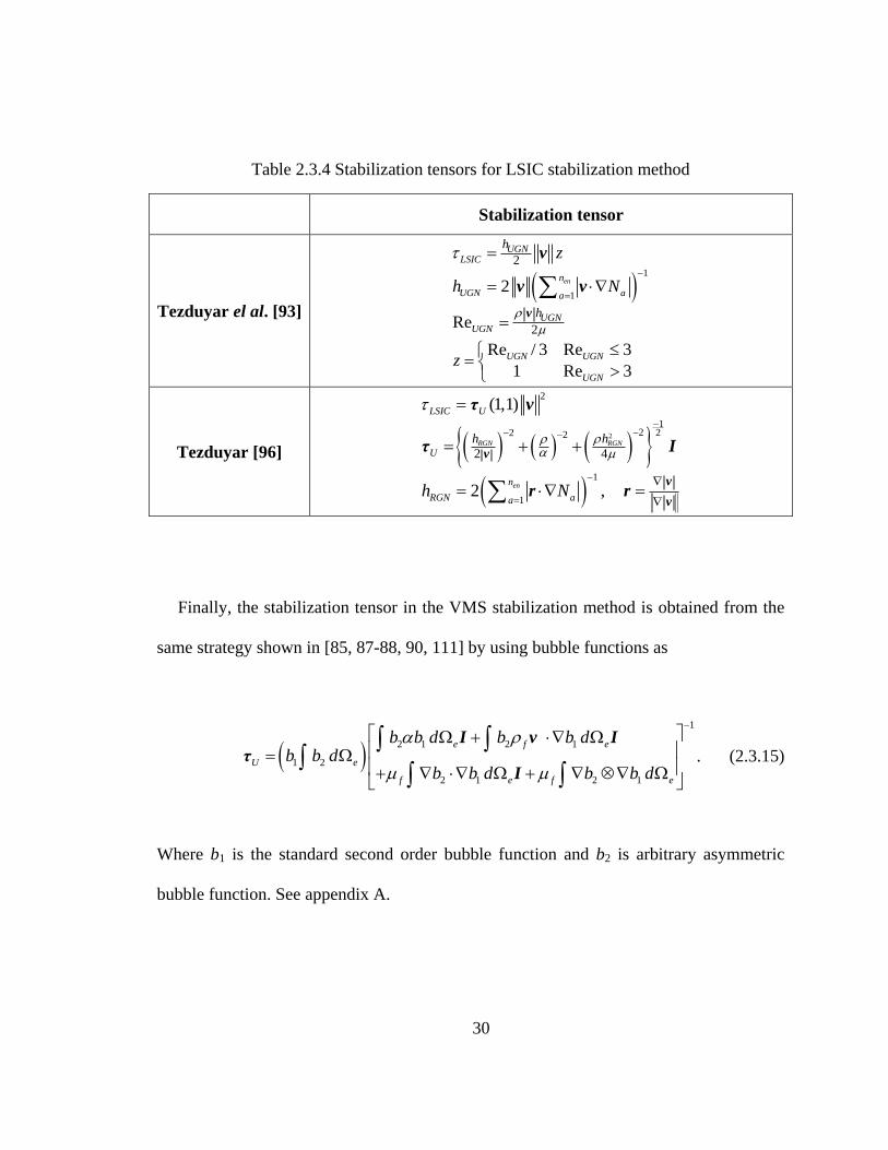
Finally, the stabilization tensor in the VMS stabilization method is obtained from the

same strategy shown in [85, 87-88, 90, 111] by using bubble functions as

1

2 1 2 1

1 2

2 1 2 1

e f e

U e

f e f e

b b d b b db b d

b b d b b d

I v Iτ

I. (2.3.15)

Where b1 is the standard second order bubble function and b2 is arbitrary asymmetric

bubble function. See appendix A.

31

2.4. Newton-Raphson method

This section shows in detail how to solve the Brinkman-penalized Navier-Stokes

equation (2.2.3) using the Newton-Raphson method. This fluid equation is a steady-state

nonlinear equation and may be expressed in the residual form as

,U U R τ u u 0 . (2.3.16)

where UR is the residual or momentum equation including the stabilization terms

,Lw L

, and u is the system response including velocity vector v and pressure p.

Equation (2.3.16) is solved iteratively by the Newton-Raphson iteration method. If the

current iterate uI is not a solution, i.e. if I I,U U R τ u u 0 , then the next iterate u

I+1 is

computed by equating the first-order Taylor series expansion of UR about u

I to zero, i.e.

I+1 I+1 I+1 I+1

I I

, ,

,

U U U U

UU U

D

D

R τ u u R τ u u u u

RR τ u u u 0

u

(2.3.17)

where UD DR u is the tangent operator and δu is the incremental response which is

determined from the following equation

I I,UU U

D

D

Ru R τ u u

u. (2.3.18)

32

Upon evaluation of the incremental response δu, the next iterate uI+1

is updated form the

sum

I 1 I u u u . (2.3.19)

The process of evaluating the residual UR and updating the response u continues until the

solution converges.

2.4.1. Reynolds-ramping initial guess for Newton-Raphson method

Selecting appropriate initial value u0 is very critical for using Newton-Raphson

iterative method because this method may fail to converge if the initial value is too far

from the true solution. Particularly, the solvability is very sensitive to the initial value

when the governing equation is highly nonlinear. During the topology optimization

progress, the complex structures make the Brinkman-penalized Navier-Stokes equation

significantly nonlinear even if the Reynolds number is not high. Therefore, we need a

very robust scheme to set up proper initial values to obtain the true solution without

failure. In fluid dynamics problems, the nonlinear terms are approximately proportional

to the Reynolds number; therefore, one can select appropriate initial value by iteratively

solving less nonlinear problem as shown in Figure 2.4.1.

33

Figure 2.4.1. Flow chart of the Reynolds-ramping initial guess

34

1) Start fluid analysis for a low Reynolds number with arbitrary initial values

2) Get a converged solution for the Reynolds number.

3) If the solution does not converge, try to solve a lower Reynolds number flow.

4) If the solution converges, use that solution as the initial values for a bigger

Reynolds number flow

Repeat 2), 3) and 4) until the full Reynolds number is reached.

2.4.2. Stabilization tensor update scheme

Two options can be considered regarding the update of the stabilization tensors during

the Newton-Raphson iteration. First, the values of the stabilization tensors are not fixed

and their variations are taken into account in calculating the Jacobian matrix in each

Newton-Raphson iteration. With this scheme, the implicit derivative DτU/Du must be

calculated as shown in equation (2.3.20).

Iat =

U U U U

U

D D

D D

u u

R R τ R

u τ u u (2.3.20)

This process is referred to as “simultaneous update scheme”. Second, the value of the

stabilization tensor is fixed based on the previous Newton-Raphson iteration result uI

without taking its variation into account when calculating the Jacobian matrix. Then, the

Jacobian matrix is determined as:

35

Iat =

U UD

D

u u

R R

u u. (2.3.21)

This is referred to as “iteration-lagging update scheme”.

Of the two update schemes, the former simultaneous update scheme is strongly

recommended for the topology optimization. Analytically calculating the variation of the

stabilization tensor is complex and requires more computational cost in each Newton-

Raphson iteration. However, the Jacobian matrix UD

D

R

u becomes more accurate with the

term U U

U

D

D

R τ

τ uand, as a result, the first scheme requires fewer Newton-Raphson

iterations than the second scheme.

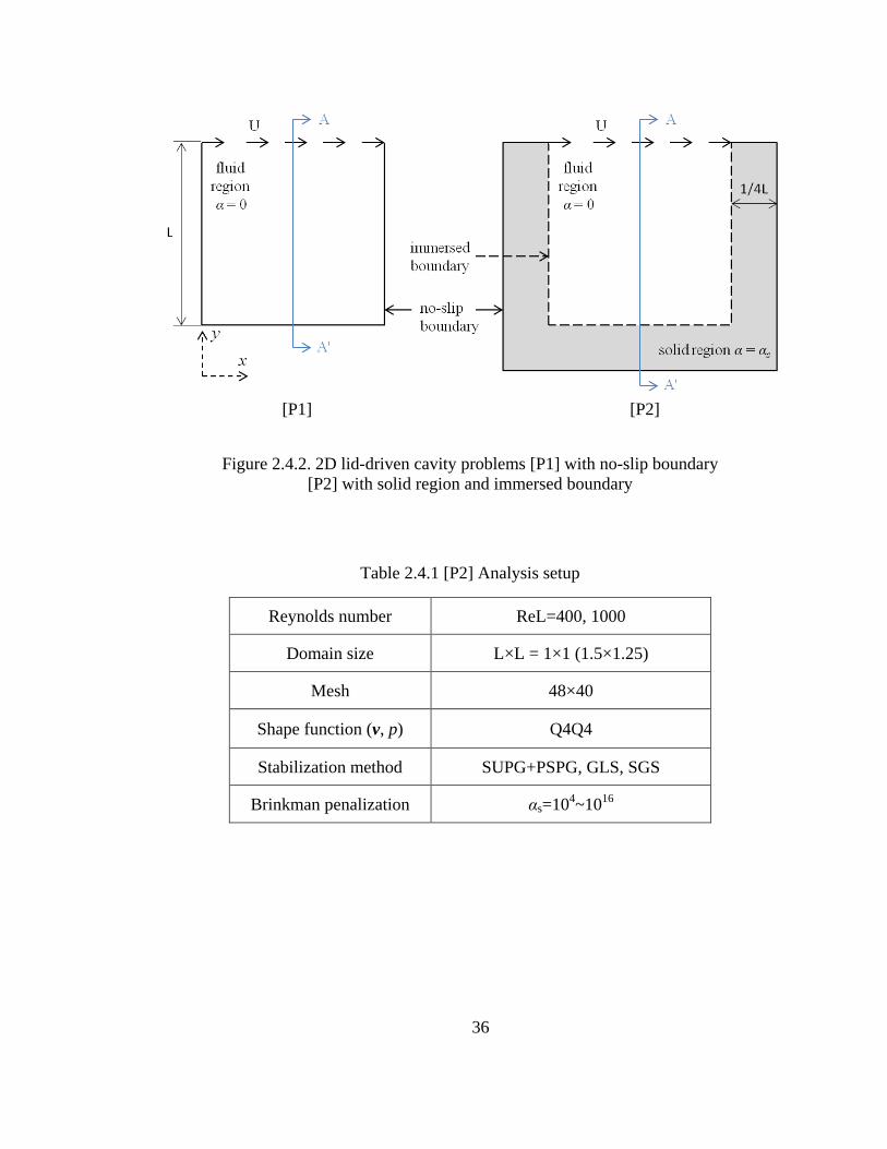
To verify the analysis method described in this chapter, an example problem P2 is

examined. As shown in Figure 2.4.2 and Table 2.4.1, immersed boundaries and a solid

region are implemented instead of the no-slip boundary condition. The Reynolds number

is 1000 and αs is set to 108. (Darcy number in the solid region is 10

-8.) The Reynolds-

ramping initial guess scheme is used to properly set the initial guess and get the true

solution. Flow analyses for ReL=10, 100, 400 and 700 flows sequentially precede before

the flow analysis at ReL=1000. Figure 2.4.3 shows the convergence history during the

last three analyses for ReL=400, 700 and 1000 flow. There is no noticeable difference

during the analyses for ReL=1 and 100 flow. In this case, the simultaneous update

scheme is 28% faster than the iteration-lagging update scheme.

36

[P1] [P2]

Figure 2.4.2. 2D lid-driven cavity problems [P1] with no-slip boundary

[P2] with solid region and immersed boundary

Table 2.4.1 [P2] Analysis setup

Reynolds number ReL=400, 1000

Domain size L×L = 1×1 (1.5×1.25)

Mesh 48×40

Shape function (v, p) Q4Q4

Stabilization method SUPG+PSPG, GLS, SGS

Brinkman penalization αs=104~10

16

37

Figure 2.4.3. [P2] Convergence history according to different stabilizing tensor update

schemes: simultaneous and iteration-lagging update schemes

Besides using the simultaneous update scheme is much more important in performing

sensitivity analysis for the topology optimization. During the topology optimization, the

physical properties in the stabilization tensor, such as ρf, μf and α, are assumed to be

control parameters. Particularly, the Brinkman-penalization parameter α is a primary

control parameter with significantly large values in the solid regions. Therefore,

assuming constant stabilization tensors in each Newton-Raphson iteration without

considering UD

D

τdegrades the accuracy of the sensitivity analysis.

Whereas the simultaneous update scheme is viable in the SUPG, PSPG, GLS and SGS

methods, it is difficult to apply for the VMS stabilization method in which its

stabilization tensor is determined from the inverse of a matrix consisting of physical

38

properties and system response as shown in equation (2.3.15). Thus it is inefficient to

calculate the derivatives of the stabilization tensor with respect to system response or

physical properties, DτU/Du or DτU/Dα respectively.

Furthermore, I discovered no significant advantage of using the VMS stabilization

method with its complicated stabilization tensor calculation compared to using the SGS

method with a relatively simple stabilization tensor. Consequently, I mainly tested the

SUPG, PSPG, GLS and SGS stabilization methods for the topology optimization problem.

Still there may, however, be a room for improvement in the VMS stabilization method

based on the proper selection of the asymmetric bubble function b2 in equation (2.3.15).

Further rigorous study is needed to implement the VMS stabilization method.

2.5. Numerical issues

This section presents a guideline to pre-assign the Brinkman penalization parameter αs,

and discusses numerical instability at the free-fluid and solid interfaces. The pre-assigned

value of αs influences the accuracy of system analysis and further the design sensitivity

calculation. The local instability does not degrade the overall solution in system analysis,

but I mention here because the instability becomes problematic later in the sensitivity

analysis at the design optimization level.

2.5.1. Lower limit of the Brinkman penalization parameter

To obtain accurate solution at the system analysis level is a primary issue because the

accuracy of the design sensitivity mainly depends on the accuracy of the system analysis.

39

When solving the Brinkman-penalized Navier-Stokes equation, the error estimate of the

velocity field in the H1-norm over the whole domain is the order of 1/4

f s O , while

the L2-norm of the velocity inside the solid body is 3/4

sO as proved in [43-44]. In

theory, the higher αs is set, the smaller the mathematical error is. In practice, too large of a

value for αs however makes the contribution from the convection and diffusion terms

negligibly small compared to the Brinkman penalization term. This would destroy the

conditioning of the Jacobian matrix. Furthermore, too large of a value for αs would cause

inaccurate sensitivity analysis because it would worsen the condition of the multiplication,

T

U U

R R

u, Therefore, the value of αs must be assigned within a proper range.

Several Brinkman penalization parameters, from 104 to 10

16, are tested for the 2D lid-

driven cavity problem that includes a solid region as shown in Figure 2.4.2. Q4Q4

element with square mesh is used. The mesh size for problem P1 and P2 is 32×32 and

48×40, respectively to have the same element length scale. The Reynolds number is 400.

Figure 2.5.1 shows different horizontal velocity results depending on the value of αs.

When αs is greater than 106 (the Darcy number in the solid region is 10

-6), the solutions

are well converged to the original solution calculated with no-slip boundary conditions.

40

(a) (b)

Figure 2.5.1. [P2] Horizontal velocity at section A-A′ according to αs (ReL=400,

SUPG+PSPG) (a) global velocity (b) local view at fluid-solid interface

Figure 2.5.2. [P2] Convergence histories according to αs (ReL=400, SUPG+PSPG)

41

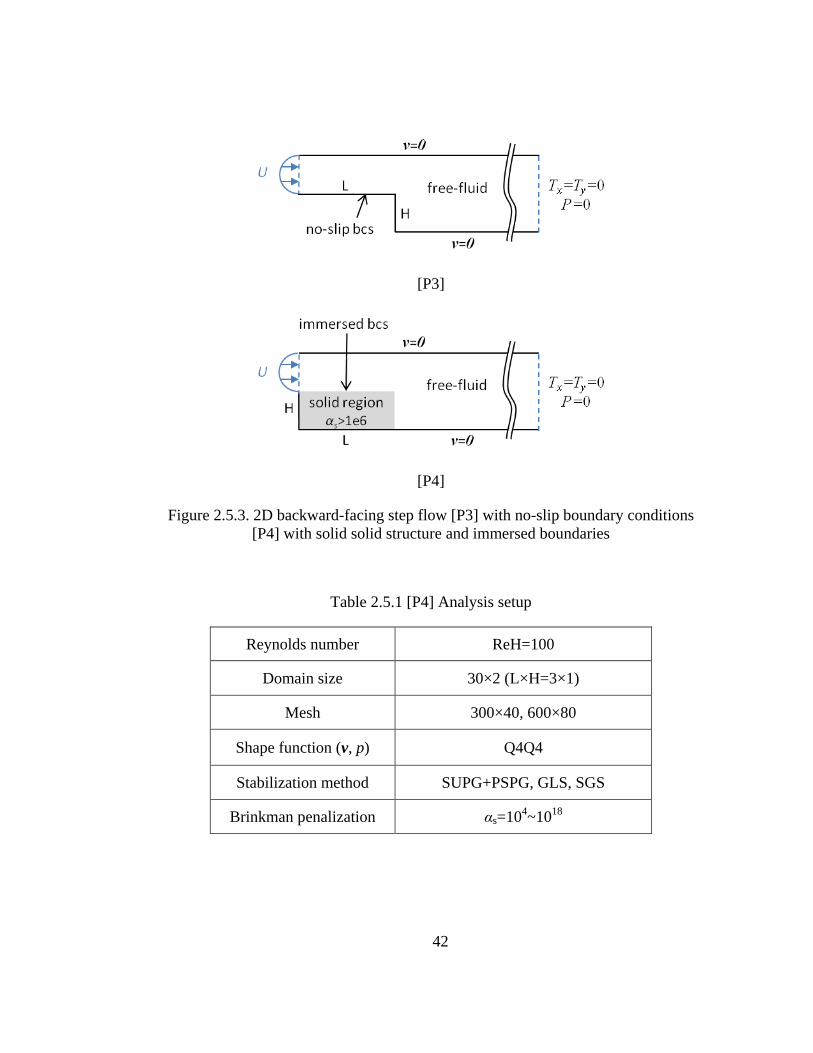
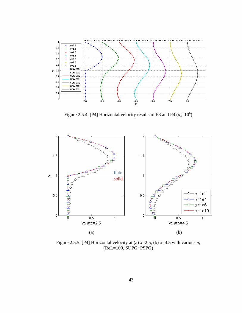
In the same manner, 2D backward-facing step flow analysis is performed first with no-

slip boundary conditions and second with immersed boundary conditions and solid region.

αs is set to from 102 to 10

18. Analysis domain and boundary conditions are described in

Figure 2.5.3 and Table 2.5.1. Q4Q4 element with 300×40 or 600×80 square mesh is used

for problems P4 and a equivalent-size mesh is used for problem P3. The Reynolds

number ReH is set to 100. To verify the analysis method, COMSOL 3.5a is used to solve

problem P3 while the solution of P4 is obtained by using my own codes; Figure 2.5.4 and

Figure 2.5.5 show the two results. Again, when αs is greater than 106, the solutions of P4

are well converged to the solution of P3 (with no-slip boundary condition).

Figure 2.5.1 and Figure 2.5.6 present that the zero-velocity condition inside the solid

structure and no-slip boundary condition at the immersed boundary (fluid-solid interface)

are reasonable realized as the value of the Brinkman penalization parameter increases.

The convergence of Newton-Raphson iteration is slightly better when a smaller value of

the Brinkman penalization parameter as shown in Figure 2.5.2 and Figure 2.5.7, yet

overall they show good convergence histories. In conclusion, several tests in other

configurations show αs=106 (the Darcy number in the solid region is 10

-6) is the proper

lower limit for reasonable use of the Brinkman-penalization method.

42

[P3]

[P4]

Figure 2.5.3. 2D backward-facing step flow [P3] with no-slip boundary conditions

[P4] with solid solid structure and immersed boundaries

Table 2.5.1 [P4] Analysis setup

Reynolds number ReH=100

Domain size 30×2 (L×H=3×1)

Mesh 300×40, 600×80




18

43

Figure 2.5.4. [P4] Horizontal velocity results of P3 and P4 (αs=106)

(a) (b)

Figure 2.5.5. [P4] Horizontal velocity at (a) x=2.5, (b) x=4.5 with various αs

(ReL=100, SUPG+PSPG)

44

(a) (b)

Figure 2.5.6. [P4] Horizontal velocity oscillation various αs (ReL=100, SUPG+PSPG)

(a) global velocity (b) local view at fluid-solid interface

Figure 2.5.7. [P4] Convergence history according to different Brinkman penalization

parameters

45

2.5.2. Numerical issues at fluid-solid interfaces (immersed boundaries)

Although the overall velocity profiles are consistent with the solutions obtained by

using the traditional no-slip boundary conditions, there sometimes exist disturbances,

such as oscillation and over-diffusion, at the immersed boundary. For example, if the

velocity profile shown in Figure 2.5.6(a) is examined again after magnifying it near the

immersed boundaries (solid-fluid interfaces), element-scale oscillations of velocity or

pressure are observed, as shown in Figure 2.5.6(b). Figure 2.5.8 describes another

example problem which shows the velocity oscillation at the immersed boundaries. A

solid obstacle lies in the middle of the analysis domain, and uniform flow motion is

applied to inlet and free-stream boundary conditions. The velocity solution obtained by

using the Brinkman penalization method is presented in Figure 2.5.9. Consistent with the

previous result of P2 and P4, the velocity profile shows good convergence when αs is

greater than 106, but the velocity oscillation at the fluid-solid interface is again discovered.

46

(a)

Reynolds number ReL=100

Domain size 3×1

Mesh 300×100, 600×200




16

(b)

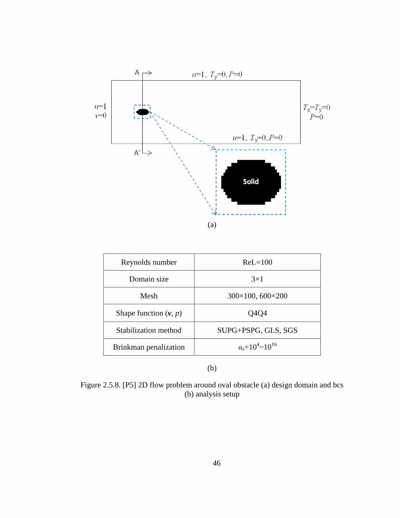
Figure 2.5.8. [P5] 2D flow problem around oval obstacle (a) design domain and bcs

(b) analysis setup

47

(a) (b)

Figure 2.5.9. [P5] Horizontal velocity results (section A-A′) accoring to the value of

Brinkman penalization parameter (a) global velcoity (b) local velocity view

(a) (b)

Figure 2.5.10. [P5] Horizontal velocity results (section A-A′) accoring to different mesh

sizes (a) global velcoity (b) local velocity view

48

In porous flow analysis, velocity oscillation at the interface between porous and solid

regions is a well-known numerical phenomenon [112]. This is because the Darcy model

inherits a conflict among the shear stress condition, mass flow rates and velocity

continuity condition at the interface. Thus, the oscillation due to the Darcy model is not a

mesh refinement problem. However, the oscillations in this study, which occur at the

immersed boundary location, are a mesh refinement problem, although the Brinkman-

penalized Navier-Stokes equation is derived based on similar porous flow physics. First,

the velocity gradient changes too sharply at the immersed boundaries for the SUPG

stabilization methods to correctly capture the velocity profile. Second, meshes used

during topology optimization process are generally non body-conforming, as shown in

Figure 2.5.8(a); therefore there are singular corner points that cause a pressure oscillation.

Figure 2.5.10 shows that the amount of oscillation is reduced with mesh refinement.

Although a denser mesh at the fluid-solid interfaces can prevent or soothe the

oscillation, it is almost impossible to apply a dense mesh for the topology optimization

problem. During the topology optimization process, the shape of the solid structure

constantly changes and accordingly, the location of the interfaces moves at each design

step. We therefore must remesh at each design step to apply a sufficiently dense mesh at

the local area, which negates all the advantages of using the fictitious domain approach

and significantly increases the computational cost.

This study also examines the possibility of reducing the oscillation by applying

different stabilization methods, such as the SUPG+PSPG, GLS and SGS stabilization

methods. The analysis results obtained using different stabilization methods are presented

from Figure 2.5.11 to Figure 2.5.16. At the global scale, the results do not differ

49

significantly from those obtained using the SUPG+PSPG, GLS and SGS stabilization

methods. However, the magnified local velocity view at the solid-fluid interfaces reveals

differences between the three solutions.

The GLS stabilization method generally results in the smaller oscillation than the

SUPG+PSPG stabilization method, regardless of the value of the Brinkman penalization

parameter α. This result seems to be contrary to the theory because the GLS stabilization

magnifies the oscillation produced by the SUPG method when the 1D convection-

diffusion-reaction (CDR) example is solved [75]. This is probably because there are two

main differences between the CDR example and these problems P2, P4 and P5. First, the

high reaction is not constantly positive in the direction of flow stream. Second, not only

the high reaction term but also corner singularities result in the oscillation. The SGS

stabilization method produces slightly over-diffused solutions preventing oscillated

solutions in case P2. However, this cannot be generalized since, in other cases, the SGS

produces more severe oscillations than the SUPG+PSPG stabilization method. For

example, the velocity profile obtained by using the SGS stabilization method shows the

worst oscillation at the immersed boundaries in cases P4 and P5.

The difference in solutions obtained by different stabilization tensors is not significant

although the Newton-Raphson convergence ratios are slightly inconsistent. Also, the

effect of the LSIC stabilization method is negligible because the Reynolds number tested

is not sufficiently high. Also, it should be mentioned that the magnitude of oscillation

depends on the value of the Brinkman penalization parameter. As αs increases, the

obtained solutions first show over-diffusion, then large oscillation and finally small

oscillation.

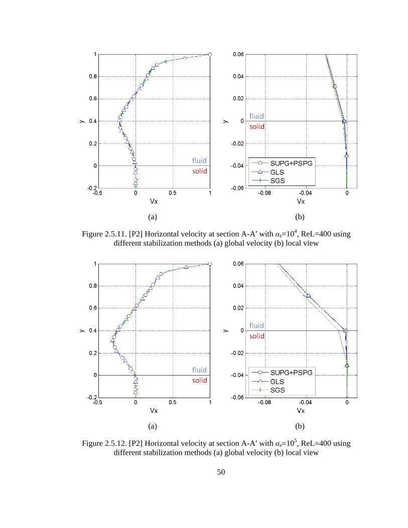
50

(a) (b)


different stabilization methods (a) global velocity (b) local view

(a) (b)



51

(a) (b)



(a) (b)

Figure 2.5.14. [P2] Horizontal velocity at section A-A′ with αs=1010

, ReL=400 using


52

(a) (b)

Figure 2.5.15. [P4] Horizontal velocity oscillation according to stabilization methods (a)

global velocity (b) local velocity view at fluid-solid interface

(a) (b)

Figure 2.5.16. [P5] Horizontal velocity results (section A-A′) accoring to different

stabilization methods (a) global velcoity (b) local velocity view

53

Various analyses with different configurations indicate that the GLS stabilization

method generally produces the best solution with the weakest oscillation. More

mathematically rigorous study of how each stabilization method effects on the oscillation

phenomenon is needed. Also, too small of a value for the Brinkman penalization

parameter not only prevents a converged solution, but also increases the magnitude of

oscillation. Mathematical verification of the relations is left for further research.

Finally, it should be noted that this local instability might later spoil the optimization

solution. This instability does not degrade the overall solution at the level of system

analysis. Brinkman penalization is mathematically justified from the viewpoint of system

analysis [43-44]. The relation between the local oscillation and other numerical

instabilities observed during the optimization process will be discussed in detail in

section 3.3.3.

2.6. Summary

In this chapter, I revisited a fictitious design approach to analyze the physics in fluid

and solid regions together with one equation by explaining the concept of the Brinkman-

penalized Navier-Stokes equation and the homogenized thermal transport equation.

SUPG, PSPG, GLS, VMS and LSIC stabilization methods and various schemes to

calculate their stabilization tensors were briefly introduced and tested. The Newton-

Raphson method for solving the nonlinear equation was described in detail. Reynolds-

Ramping initial guess strategy and a simultaneous stabilization tensor update scheme

54

were presented, which are essential in obtaining robust and fast solutions for highly

nonlinear topology optimization problems.

With example problems, a guideline to set a proper lower bound of the Brinkman

penalization parameter was presented. When the Brinkman penalization parameter is

greater than 106 (Da=10

-6), the zero-velocity condition in the solid regions and the no-slip

boundary condition at solid boundaries are generally satisfied. Velocity and pressure

oscillations at the fluid-solid interfaces were presented and investigated.

These numerical instabilities are a mesh-refinement problem unlike the oscillation

occurring in porous flow analysis. This oscillation becomes stronger as the Reynolds

number increases and a coarser mesh is used. Also, the magnitude of oscillation depends

on the value of the Brinkman penalization parameter increases. As αs increases, the

obtained solutions show over-diffusion, large oscillation and small oscillation,

sequentially.

Although the solutions obtained from different stabilization methods are overall very

similar to each other, discrepancies are found near fluid-solid interfaces. The

SUPG+PSPG and GLS stabilization methods produce the velocity and pressure

oscillation, while the SGS stabilization method produces the strongest oscillation or an

over-diffused solution. No notable difference is found due to the change of a stabilization

tensor.

55

CHAPTER 3

3. TOPOLOGY OPTIMIZATION OF NAVIER-STOKES FLOW PROBLEMS

3.1. Introduction

This chapter investigates the topology optimization method of Navier-Stokes flow

systems, extending previous studies concerning Stokes flow systems [45-46, 51, 100-

102]. Topology optimization method involves a great number of discrete design variables;

therefore a very efficient algorithm should be implemented to solve topology

optimization problems. In order to use gradient-based optimization methods which are

typically efficient in problems with many design variables, the discrete design variables

are relaxed by using continuous interpolation functions [1, 113]. Then the derivatives of

an objective function with respect to the design variables are calculated. The adjoint

sensitivity method for a steady state nonlinear system [114] is applied to calculate the

derivatives.

Numerical issues, such as element-scale cavities and boundary oscillation

phenomenon, which deteriorate the convergence property, are presented and investigated.

These numerical issues have not appeared or been discussed in previous topology

56

optimization studies of Stokes flow systems or low-Reynolds number flow systems [45-

46, 51, 100-102]. Filtering methods [115-117], different stabilized finite element methods

and a move-limit scheme are suggested and examined to overcome the numerical issues.

Unlike the well-known checkerboard pattern in topology optimization [1, 113], filtering

methods such as the density filter and the sensitivity filter do not completely suppress the

cavities and boundary oscillations. Instead, these numerical instabilities are successfully

circumvented with the easy implementation of a move-limit scheme. Finally, 2D and 3D

design problems are presented and physically interpreted. The objective function is the

minimization of kinetic energy dissipation or drag minimization.

The outline of Chapter 3 is as follows. Section 3.2 presents the sensitivity analysis

with RAMP interpolation function and the adjoint sensitivity method. Section 3.3

investigates numerical instabilities and suggests how to resolve them. After presenting

several 2D and 3D design problems in section 3.4, summaries and observations are given

in section 3.5.

3.2. Sensitivities analysis for nonlinear problems

Topology optimization determines optimized distribution of two-phase material, such

as solid and void (free-fluid), in a design domain. The material phase is determined by

local material properties, which are controlled by a local design variable φ(r) which is

zero in free-fluid regions and unity in the solid regions. For example, if a local design

variable is unity (φ=1), the local element or the local point r is in the solid region Ωs

having solid material properties. On the contrary, if a local design variable is zero (φ=0),

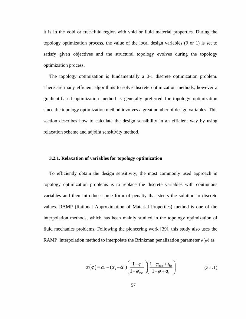
57

it is in the void or free-fluid region with void or fluid material properties. During the

topology optimization process, the value of the local design variables (0 or 1) is set to

satisfy given objectives and the structural topology evolves during the topology

optimization process.

The topology optimization is fundamentally a 0-1 discrete optimization problem.

There are many efficient algorithms to solve discrete optimization methods; however a

gradient-based optimization method is generally preferred for topology optimization

since the topology optimization method involves a great number of design variables. This

section describes how to calculate the design sensibility in an efficient way by using

relaxation scheme and adjoint sensitivity method.

3.2.1. Relaxation of variables for topology optimization

To efficiently obtain the design sensitivity, the most commonly used approach in

topology optimization problems is to replace the discrete variables with continuous

variables and then introduce some form of penalty that steers the solution to discrete

values. RAMP (Rational Approximation of Material Properties) method is one of the

interpolation methods, which has been mainly studied in the topology optimization of

fluid mechanics problems. Following the pioneering work [39], this study also uses the

RAMP interpolation method to interpolate the Brinkman penalization parameter α(φ) as

min αs s f

min α

11( )

1 1

q

q

(3.1.1)

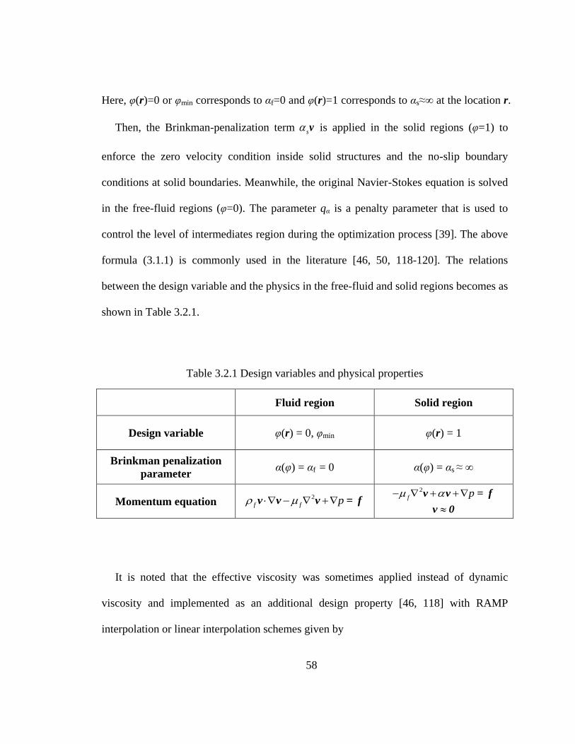
58

Here, φ(r)=0 or φmin corresponds to αf=0 and φ(r)=1 corresponds to αs≈∞ at the location r.

Then, the Brinkman-penalization term s v is applied

in the solid regions (φ=1) to

enforce the zero velocity condition inside solid structures and the no-slip boundary

conditions at solid boundaries. Meanwhile, the original Navier-Stokes equation is solved

in the free-fluid regions (φ=0). The parameter qα is a penalty parameter that is used to

control the level of intermediates region during the optimization process [39]. The above

formula (3.1.1) is commonly used in the literature [46, 50, 118-120]. The relations

between the design variable and the physics in the free-fluid and solid regions becomes as

shown in Table 3.2.1.

Table 3.2.1 Design variables and physical properties


Design variable φ(r) = 0, φmin φ(r) = 1


parameter α(φ) = αf = 0 α(φ) = αs ≈ ∞

Momentum equation 2

f f p v v v = f 2

f p

v v = f

v 0

It is noted that the effective viscosity was sometimes applied instead of dynamic

viscosity and implemented as an additional design property [46, 118] with RAMP

interpolation or linear interpolation schemes given by

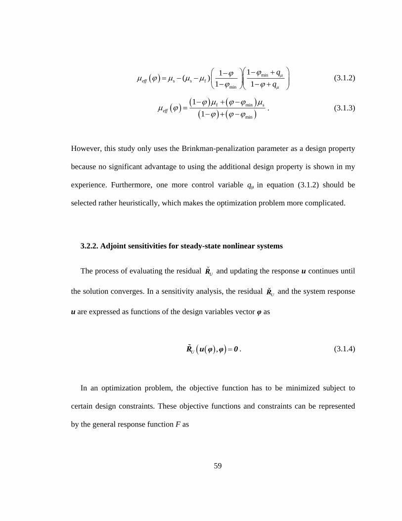
59

min

s s f

min

11( )

1 1eff

q

q

(3.1.2)

f min s

min

1

1eff

. (3.1.3)

However, this study only uses the Brinkman-penalization parameter as a design property

because no significant advantage to using the additional design property is shown in my

experience. Furthermore, one more control variable qμ in equation (3.1.2) should be

selected rather heuristically, which makes the optimization problem more complicated.

3.2.2. Adjoint sensitivities for steady-state nonlinear systems

The process of evaluating the residual UR and updating the response u continues until

the solution converges. In a sensitivity analysis, the residual UR and the system response

u are expressed as functions of the design variables vector φ as

,U R u φ φ 0 . (3.1.4)

In an optimization problem, the objective function has to be minimized subject to

certain design constraints. These objective functions and constraints can be represented

by the general response function F as

60

,F Gφ u φ φ (3.1.5)

Notice that the dependence of the response function F on the design vector φ is rewritten

using the function G so as to isolate its implicit dependence on φ through u(φ) from the

explicit dependence on φ.

Gradient-based optimization schemes require the derivatives of the response functions

with respect to the design variable, which can be computed from (3.1.5) as

i i i

DF G D G

D D

u

u. (3.1.6)

In the above equation, the derivatives ∂G/∂u and ∂G/∂φi are explicit quantities, whereas

the derivative Du/Dφi is an implicit quantity because the system response is implicitly

defined through equation (3.1.4).

In the direct differentiation approach, the implicit derivative Du/Dφi is evaluated and

then the sensitivities are obtained from equation (3.1.6). This is accomplished by

differentiating equation (3.1.4) with respect to the individual design parameters φi, which,

after some rearranging, yields

U U

i i

D

D

R Ru

u. (3.1.7)

The above equation forms a pseudo-problem for the evaluation of the response

sensitivity Du/Dφi resulting from the pseudo-load U iD D R , Note here that the

61

operator in the pseudo-problem is identical to the tangent operator in the Newton-

Raphson analysis of the primal problem (2.3.18). In a finite element analysis, this

reappearance of the tangent operator allows the decomposed tangent stiffness matrix

resulting from the iterative solution of u to be used to solve equation (3.1.7) efficiently

for the implicit response sensitivity Du/Dφi. Hence, the evaluation of the derivative

Du/Dφi requires only the formation of the pseudo-load vector U i R .

Adjoint sensitivities are obtained via the Lagrange multiplier method, where the

implicit response sensitivity Du/Dφi is eliminated from equation (3.1.6). Equations

(3.1.4) and (3.1.5) are combined to define the augmented functional

ˆ , ,U UF G φ u φ φ λ φ R u φ φ (3.1.8)

where λU(φ) is the Lagrange multiplier and u is a solution to equation(3.1.9). Note here

that F F since U R 0 from equation (3.1.4). Differentiation of the above with respect

to the individual design parameters φi yields

ˆ

U U UU

i i i i i i

DDF G D G D

D D D D

λ R Ru uR λ

u u (3.1.10)

Here, I note again that î iDF D DF D since again

U R 0 .

To isolate the implicit response sensitivities, I separate equation (3.1.10) into two

terms

62

ˆ ˆˆ

E I

i i i

DF DFDF

D D D (3.1.11)

where Ê iDF D and ˆ

I iDF D are the explicit and implicit terms, respectively, defined

as

ˆ

UEU

i i i

DF G

D

Rλ (3.1.12)

ˆ

T

UIU

i i

DF D G

D D

Ruλ

u u (3.1.13)

The implicit part Î iDF D is eliminated from the sensitivity expression by defining

the Lagrange multiplier λU, so that equation (3.1.13) equals zero. Once this λU is

determined, the unknown derivative Du/Dφi is eliminated from the sensitivity expression

and the sensitivities are evaluated from the remaining explicit quantity (i.e.

equation(3.1.12)). Annihilation of the implicit term in equation (3.1.13) yields the

following adjoint problem for the adjoint response Lagrange multiplier λU.

T

UU

G

Rλ

u u (3.1.14)

where ∂G/∂u is deemed the adjoint load. Once the adjoint response λU is evaluated, the

sensitivity expression reduces to

63

ˆ

UU

i i i

DF G

D

Rλ . (3.1.15)

Here, I note that the operator that appears in the adjoint problem is the transpose of the

Newton-Raphson tangent operator used to obtain δu.

The adjoint method requires the solution of one adjoint problem for each response

function F, whereby the sensitivity is computed from equation (3.1.15). Therefore, it is

very efficient when the number of response functions is small compared with the number

of design parameters. If this ratio is reversed, the direct differentiation is generally

preferred [114].


This section presents a topology optimization example problem of Navier-Stokes flow

systems and discusses numerical instabilities in the optimization process which are not

presented in previous studies of topology optimization for Stokes flow systems [45-46,

51, 100-102]. To clarify the cause of these instabilities, adjoint sensitivities are first

compared to finite difference sensitivities, and then the effect of numerical issues in the

system analysis, which is discussed in section 2.5.2, is confirmed. To circumvent these

numerical instabilities, filtering methods, such as the density filter and the sensitivity

filter [35, 115-117], are evaluated and a move-limit approach is suggested.

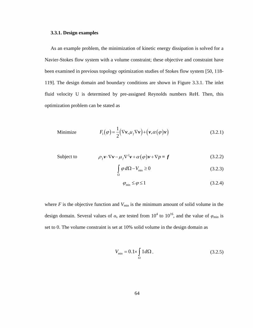
64

3.3.1. Design examples

As an example problem, the minimization of kinetic energy dissipation is solved for a

Navier-Stokes flow system with a volume constraint; these objective and constraint have

been examined in previous topology optimization studies of Stokes flow system [50, 118-

119]. The design domain and boundary conditions are shown in Figure 3.3.1. The inlet

fluid velocity U is determined by pre-assigned Reynolds numbers ReH. Then, this

optimization problem can be stated as

Minimize 1

1, ,

2fF v v v v (3.2.1)

Subject to 2

f f p v v v v = f (3.2.2)

min 0d V

(3.2.3)

min 1 (3.2.4)

where F is the objective function and Vmin is the minimum amount of solid volume in the

design domain. Several values of αs are tested from 104 to 10

16, and the value of φmin is

set to 0. The volume constraint is set at 10% solid volume in the design domain as

min 0.1 1V d

. (3.2.5)

65

(a)

Reynolds number ReH = 0.001, 10, 100, 1000

Domain size L×H = 1.5×1

Mesh 240×160, 480×320

Shape function (v, p, T) Q4Q4

Stabilization method GLS

Brinkman penalization αs = 104-10

16

(b)

Optimizer SLP, MMA

Shape function ( φ ) Q4, U1

Interpolation function RAMP

Filtering method density filter, sensitivity filter

(c)

Figure 3.3.1 [P6] 2D design example (a) design domain and boundary conditions

(b) analysis setup (c) optimization setup

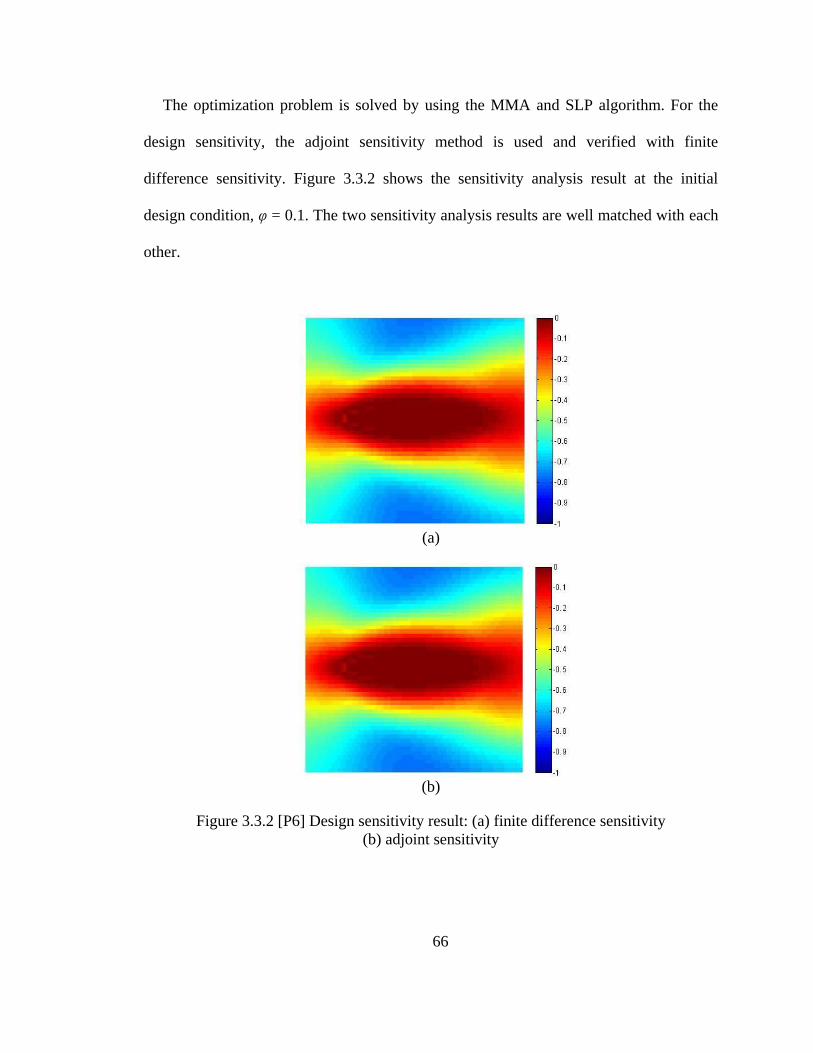
66

The optimization problem is solved by using the MMA and SLP algorithm. For the

design sensitivity, the adjoint sensitivity method is used and verified with finite

difference sensitivity. Figure 3.3.2 shows the sensitivity analysis result at the initial

design condition, φ = 0.1. The two sensitivity analysis results are well matched with each

other.

(a)

(b)

Figure 3.3.2 [P6] Design sensitivity result: (a) finite difference sensitivity

(b) adjoint sensitivity

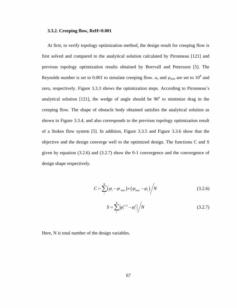
67

3.3.2. Creeping flow, ReH=0.001

At first, to verify topology optimization method, the design result for creeping flow is

first solved and compared to the analytical solution calculated by Pironneau [121] and

previous topology optimization results obtained by Borrvall and Petersson [5]. The

Reynolds number is set to 0.001 to simulate creeping flow. αs and φmin are set to 108 and

zero, respectively. Figure 3.3.3 shows the optimization steps. According to Pironneau’s

analytical solution [121], the wedge of angle should be 90o to minimize drag in the

creeping flow. The shape of obstacle body obtained satisfies the analytical solution as

shown in Figure 3.3.4, and also corresponds to the previous topology optimization result

of a Stokes flow system [5]. In addition, Figure 3.3.5 and Figure 3.3.6 show that the

objective and the design converge well to the optimized design. The functions C and S

given by equation (3.2.6) and (3.2.7) show the 0-1 convergence and the convergence of

design shape respectively.

min max

N

i i

i

C N (3.2.6)

1

NI I

i i

i

S N (3.2.7)

Here, N is total number of the design variables.

68

(a) (c)

(b) (d)

Figure 3.3.3 [P6] Design process, ReH=0.001 (a) initial design (b) 5st step (c) 10

th step

(d) 50th

step

Figure 3.3.4 [P6] Optimization result, ReH=0.001

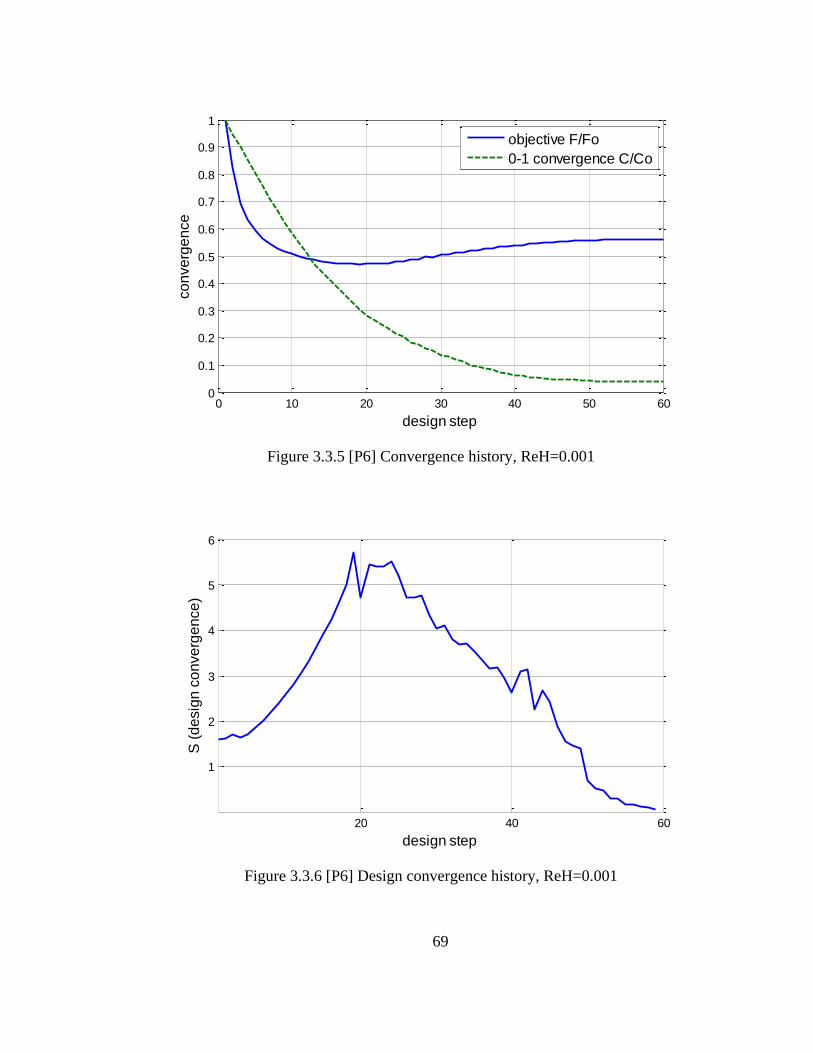
69

Figure 3.3.5 [P6] Convergence history, ReH=0.001

Figure 3.3.6 [P6] Design convergence history, ReH=0.001

0 10 20 30 40 50 600

0.1

0.2

0.3

0.4

0.5

0.6

0.7

0.8

0.9

1

design step

co

nve

rge

nce

objective F/Fo

0-1 convergence C/Co

20 40 60

1

2

3

4

5

6

design step

S (

de

sig

n c

on

ve

rge

nce

)

70

3.3.3. Fluctuation at the boundaries

Now the same optimization problem shown in section 3.3.1 is tested with a higher

Reynolds number. ReH is set to 100 with the same volume constraint 0.1. αs and φmin are

again set to 106 and zero, respectively. Either MMA or SLP algorithm is used as an

optimizer. Figure 3.3.7 shows the design history. At the initial stage, the design

converges very well as shown in Figure 3.3.7(a)-(d) before solid elements and void (free-

fluid) elements are first adjacent. From this point, the design starts fluctuating at the

solid-fluid interfaces and generates element-scale cavities as shown in Figure 3.3.7(e)-(h).

As a result, the design no longer converges as shown in Figure 3.3.8 and Figure 3.3.9. It

is noted that this numerical instability typically occurs when a large penalization term is

used or when a high Reynolds number flow is solved.

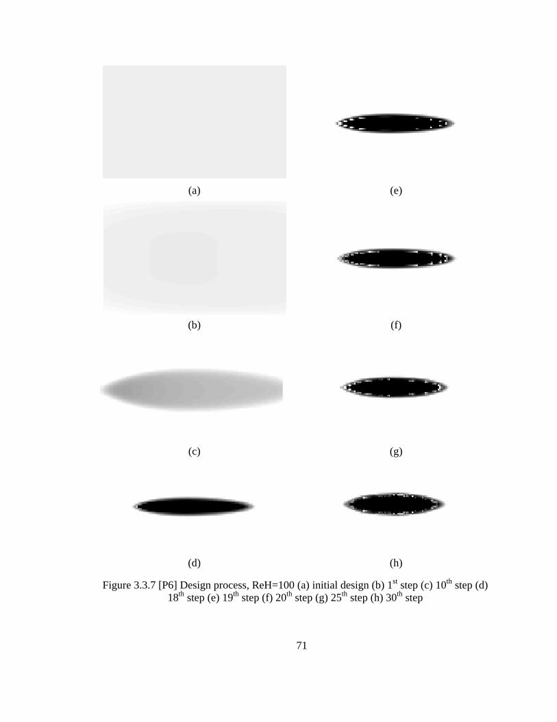
71

(a) (e)

(b) (f)

(c) (g)

(d) (h)

Figure 3.3.7 [P6] Design process, ReH=100 (a) initial design (b) 1st step (c) 10

th step (d)

18th

step (e) 19th

step (f) 20th

step (g) 25th

step (h) 30th

step

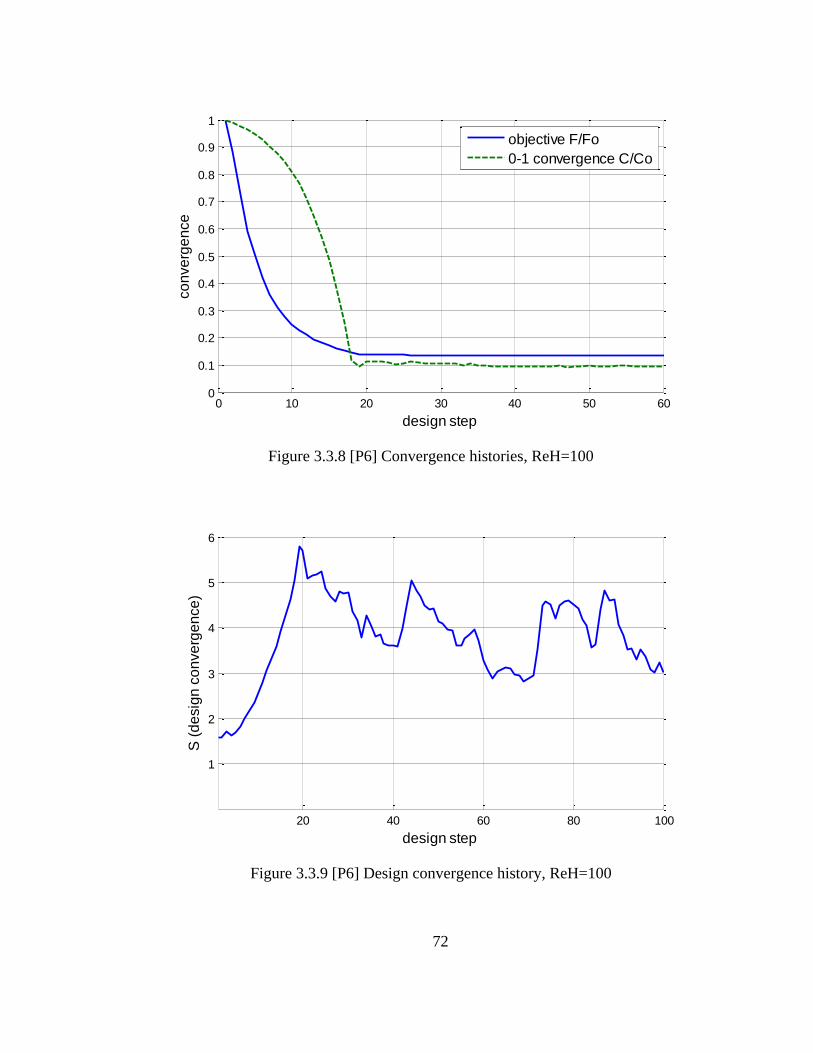
72

Figure 3.3.8 [P6] Convergence histories, ReH=100

Figure 3.3.9 [P6] Design convergence history, ReH=100

0 10 20 30 40 50 600

0.1

0.2

0.3

0.4

0.5

0.6

0.7

0.8

0.9

1

design step

co

nve

rge

nce

objective F/Fo


20 40 60 80 100

1

2

3

4

5

6

design step

S (

de

sig

n c

on

ve

rge

nce

)

73

Generally speaking, there are three possible problems that cause this numerical issue

preventing design convergence: (1) errors in the sensitivity analysis, (2) errors in the

optimizer and (3) errors in the system analysis. To clarify the reason for these boundary

oscillations and cavities, the adjoint sensitivity values at the optimization step when

design oscillation arises, and where cavities first appear, are first compared with the finite

difference sensitivity values in order to verify the adjoint sensitivity calculation. Figure

3.3.10 shows that the two sensitivity results correspond to each other, which

demonstrates that there is no error in the sensitivity analysis.

(a)

(b)

Figure 3.3.10 [P6] Design sensitivity results at 18th

step, ReH=100 (a) adjoint sensitivity

(b) finite difference sensitivity

-2000

-1500

-1000

-500

0

-2000

-1500

-1000

-500

0

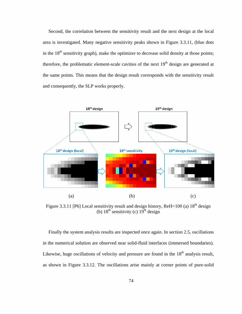
74

Second, the correlation between the sensitivity result and the next design at the local

area is investigated. Many negative sensitivity peaks shown in Figure 3.3.11, (blue dots

in the 18th

sensitivity graph), make the optimizer to decrease solid density at those points;

therefore, the problematic element-scale cavities of the next 19th

design are generated at

the same points. This means that the design result corresponds with the sensitivity result

and consequently, the SLP works properly.

(a) (b) (c)

Figure 3.3.11 [P6] Local sensitivity result and design history, ReH=100 (a) 18th

design

(b) 18th

sensitivity (c) 19th

design

Finally the system analysis results are inspected once again. In section 2.5, oscillations

in the numerical solution are observed near solid-fluid interfaces (immersed boundaries).

Likewise, huge oscillations of velocity and pressure are found in the 18th

analysis result,

as shown in Figure 3.3.12. The oscillations arise mainly at corner points of pure-solid

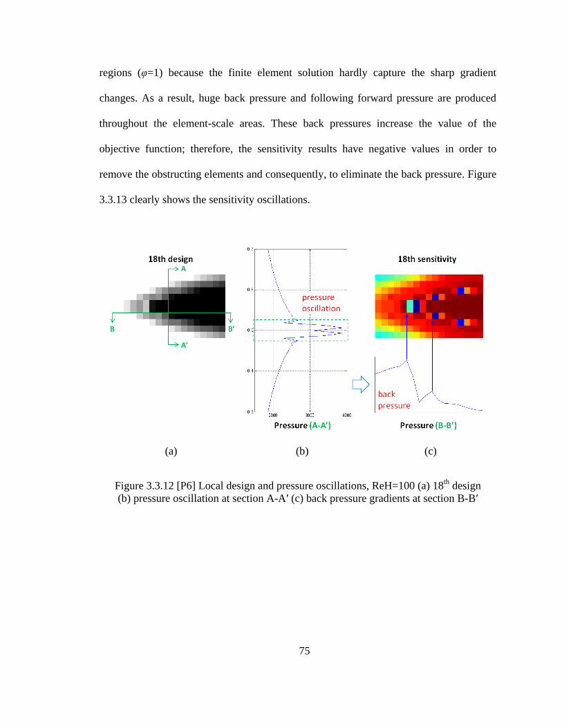
75

regions (φ=1) because the finite element solution hardly capture the sharp gradient

changes. As a result, huge back pressure and following forward pressure are produced

throughout the element-scale areas. These back pressures increase the value of the

objective function; therefore, the sensitivity results have negative values in order to

remove the obstructing elements and consequently, to eliminate the back pressure. Figure

3.3.13 clearly shows the sensitivity oscillations.

(a) (b) (c)

Figure 3.3.12 [P6] Local design and pressure oscillations, ReH=100 (a) 18th

design

(b) pressure oscillation at section A-A′ (c) back pressure gradients at section B-B′

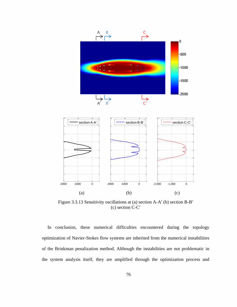
76

(a) (b) (c)

Figure 3.3.13 Sensitivity oscillations at (a) section A-A′ (b) section B-B′

(c) section C-C′

In conclusion, these numerical difficulties encountered during the topology

optimization of Navier-Stokes flow systems are inherited from the numerical instabilities

of the Brinkman penalization method. Although the instabilities are not problematic in

the system analysis itself, they are amplified through the optimization process and

-2000 -1000 0

-2000 -1000 0

-2,000 -1,000 0

section A-A' section B-B' section C-C'

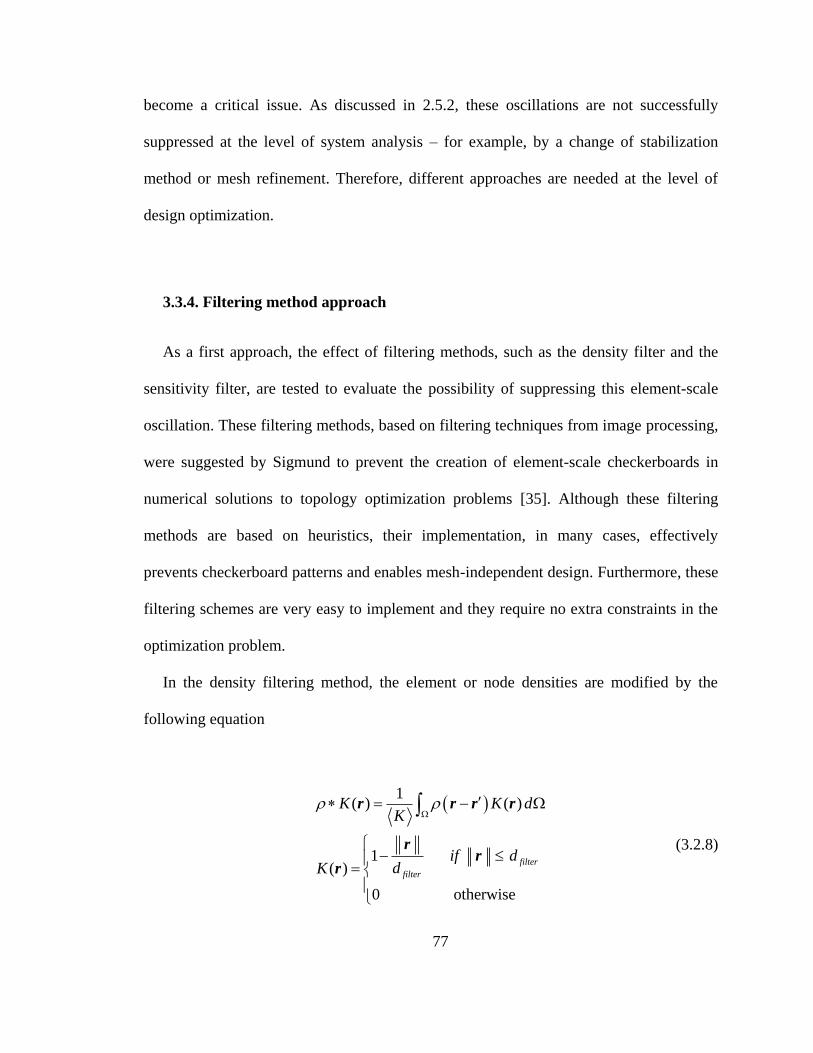
77

become a critical issue. As discussed in 2.5.2, these oscillations are not successfully

suppressed at the level of system analysis – for example, by a change of stabilization

method or mesh refinement. Therefore, different approaches are needed at the level of

design optimization.

3.3.4. Filtering method approach

As a first approach, the effect of filtering methods, such as the density filter and the

sensitivity filter, are tested to evaluate the possibility of suppressing this element-scale

oscillation. These filtering methods, based on filtering techniques from image processing,

were suggested by Sigmund to prevent the creation of element-scale checkerboards in

numerical solutions to topology optimization problems [35]. Although these filtering

methods are based on heuristics, their implementation, in many cases, effectively

prevents checkerboard patterns and enables mesh-independent design. Furthermore, these

filtering schemes are very easy to implement and they require no extra constraints in the

optimization problem.

In the density filtering method, the element or node densities are modified by the

following equation

1

( ) ( )

1( )

0 otherwise

filter

filter

K K dK

if ddK

r r r r

rr

r

(3.2.8)

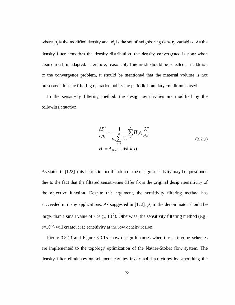
78

where e is the modified density and eN is the set of neighboring density variables. As the

density filter smoothes the density distribution, the density convergence is poor when

coarse mesh is adapted. Therefore, reasonably fine mesh should be selected. In addition

to the convergence problem, it should be mentioned that the material volume is not

preserved after the filtering operation unless the periodic boundary condition is used.

In the sensitivity filtering method, the design sensitivities are modified by the

following equation

*

1

1

1

dist( , )

N

i iNik i

k i

i

i filter

F FH

H

H d k i

(3.2.9)

As stated in [122], this heuristic modification of the design sensitivity may be questioned

due to the fact that the filtered sensitivities differ from the original design sensitivity of

the objective function. Despite this argument, the sensitivity filtering method has

succeeded in many applications. As suggested in [122], e in the denominator should be

larger than a small value of ε (e.g., 10-3

). Otherwise, the sensitivity filtering method (e.g.,

ε=10-6

) will create large sensitivity at the low density region.

Figure 3.3.14 and Figure 3.3.15 show design histories when these filtering schemes

are implemented to the topology optimization of the Navier-Stokes flow system. The

density filter eliminates one-element cavities inside solid structures by smoothing the

79

values of sharp 0-1 interfaces and, as the result, the element-scale oscillations are

suppressed as expected. However, this method does not completely resolve the overall

convergence issue because larger-scale oscillations, although they are blurry, still occur

during the optimization process disturbing convergence, as shown in Figure 3.3.14.

Sensitivity filter does not prevent the element-scale oscillation; rather it aggravates the

convergence problems, as shown in Figure 3.3.15. Figure 3.3.16 and Figure 3.3.17 show

the design results are not converged.

Despite their successful performance in preventing the checkerboard issue, these

filtering methods are not successful in preventing the boundary oscillation. This is mainly

because there are two significant differences between the typical checkerboard patterns

and the boundary oscillations. First, in the checkerboard patterns, the locations of void

and solid elements do not move at the final stage of convergence whereas the locations of

void elements (cavities in the solid structures) constantly move at each design step.

Second, due to the large value of the penalization parameter, the gradient of sensitivity

oscillation is generally much larger than the sensitivity gradients in checkerboard patterns.

Therefore, it is more difficult to smooth out sensitivity peaks by using the same

sensitivity filter method. In conclusion, the filtering methods are inappropriate to prevent

this numerical issue although they assure mesh-independent design solutions.

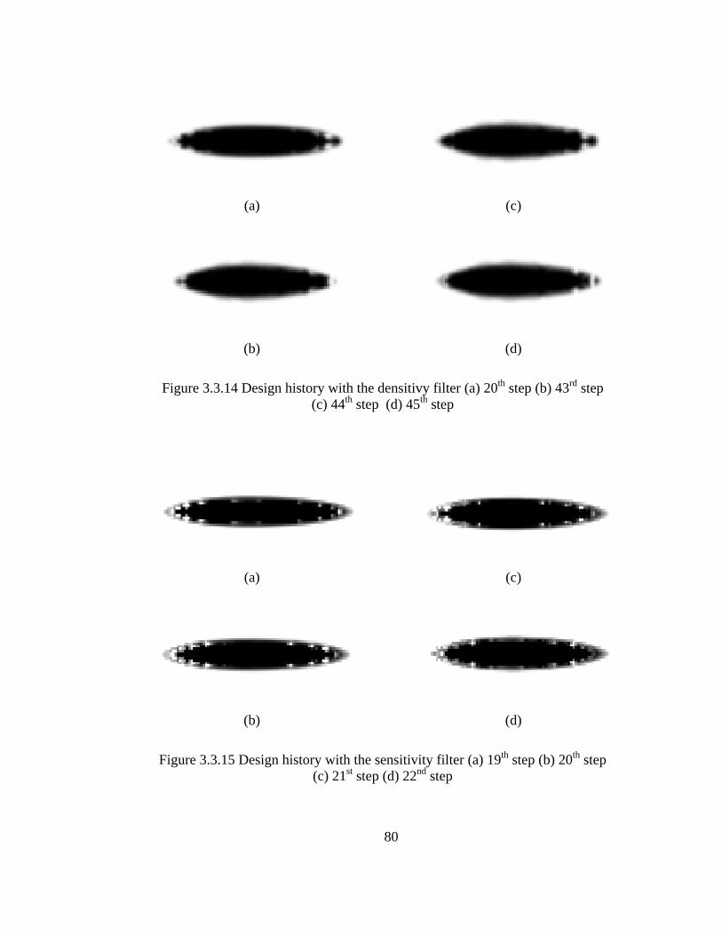
80

(a) (c)

(b) (d)

Figure 3.3.14 Design history with the densitivy filter (a) 20th

step (b) 43rd

step

(c) 44th

step (d) 45th

step

(a) (c)

(b) (d)

Figure 3.3.15 Design history with the sensitivity filter (a) 19th

step (b) 20th

step

(c) 21st step (d) 22

nd step

81

(a)

(b)

Figure 3.3.16 [P6] Design convergence histories with filters, ReH=100 (a) the density

filter, (b) the sensitivity filter

20 40 60 80 100

1

2

3

4

5

6

design step

S (

de

sig

n c

on

ve

rge

nce

)

no filter

density filter

20 40 60 80 100

1

2

3

4

5

6

design step

S (

de

sig

n c

on

ve

rge

nce

)

no filter

sensitivity filter

82

Figure 3.3.17 Objective convergence histories according to filtering schemes

3.3.5. Move-limit approach

My second approach to solve the numerical issues is to test the effect of move-limit on

the boundary oscillations. Based on the fact that the void cavities near the solid-fluid

interfaces are constantly appearing and disappearing at different locations, I set a

maximum move-limit to the design variables to prevent such sudden changes. For the

SLP optimizer, this move-limit is easily implemented with basic constraints. For the

MMA optimizer, the move-limit can be implemented by a filter given by equation (3.2.10)

83

1

min

1 1

1

max , if

min , 1 if

otherwise

i i i

i i i i

i

c c

c c

(3.2.10)

Figure 3.3.18 and Figure 3.3.19 show the design history without or with the move-

limit constraint, respectively. A 5% move-limit is applied in the previous problem. The

element-scale void-holes and resulting boundary oscillation is successfully suppressed

with the move-limit and consequently, the design converges well although the objective

does not change much, as shown in Figure 3.3.20 and Figure 3.3.21. Also, it should be

mentioned that this move-limit scheme does not significantly decelerate the speed of the

entire topology optimization of Navier-Stokes flow systems despite the need for more

design steps. When solving the nonlinear Navier-Stokes equation for the J+1th

design, the

analysis result for the previous Jth

design is generally used for the values of the initial

guess. The more the two Jth

and J+1th

designs resemble each other, the easier it is to find a

new solution. As a smaller move-limit is applied, the Jth

design and J+1th

design become

more similar, and the number of required inner loop iterations for solving the nonlinear

equation is reduced. Thus, although more outer loop design steps are needed, the fewer

inner loop iterations needed for solving the nonlinear problem compensates for the time

loss associated with the greater number of outer loop design step.

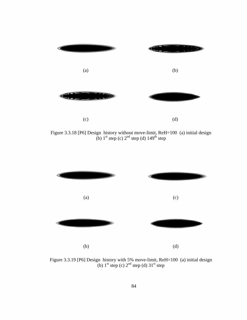
84

(a) (b)

(c) (d)

Figure 3.3.18 [P6] Design history without move-limit, ReH=100 (a) initial design

(b) 1st step (c) 2

nd step (d) 149

th step

(a) (c)

(b) (d)

Figure 3.3.19 [P6] Design history with 5% move-limit, ReH=100 (a) initial design

(b) 1st step (c) 2

nd step (d) 31

st step

18th (volume: 0.93248)

50 100 150 200

20

40

60

80

100

120

1400

0.2

0.4

0.6

0.8

1

18th Sensitivity

50 100 150 200

20

40

60

80

100

120

140

0

0.1

0.2

0.3

0.4

19th (volume: 0.93247)

50 100 150 200

20

40

60

80

100

120

1400

0.2

0.4

0.6

0.8

1

19th Sensitivity

50 100 150 200

20

40

60

80

100

120

140 -0.2

-0.1

0

0.1

0.2

0.3

0.4

20th (volume: 0.93243)

50 100 150 200

20

40

60

80

100

120

1400

0.2

0.4

0.6

0.8

1

20th Sensitivity

50 100 150 200

20

40

60

80

100

120

140-0.4

-0.2

0

0.2

0.4

167th (volume: 0.93294)

50100150200

20

40

60

80

100

120

140

167th Sensitivity

50100150200

20

40

60

80

100

120

140

0

0.2

0.4

0.6

0.8

1

-0.08

-0.06

-0.04

-0.02

0

0.02

0.04

18th (volume: 0.93248)

50 100 150 200

20

40

60

80

100

120

1400

0.2

0.4

0.6

0.8

1

18th Sensitivity

50 100 150 200

20

40

60

80

100

120

140

0

0.1

0.2

0.3

0.4

19th (volume: 0.933)

50 100 150 200

20

40

60

80

100

120

1400

0.2

0.4

0.6

0.8

1

19th Sensitivity

50 100 150 200

20

40

60

80

100

120

140

0

0.1

0.2

0.3

0.4


50 100 150 200

20

40

60

80

100

120

1400

0.2

0.4

0.6

0.8

1

20th Sensitivity

50 100 150 200

20

40

60

80

100

120

140 -0.1

0

0.1

0.2

0.3

0.4


50100150200

20

40

60

80

100

120

1400

0.2

0.4

0.6

0.8

1

49th Sensitivity

50100150200

20

40

60

80

100

120

140

-0.2

0

0.2

0.4

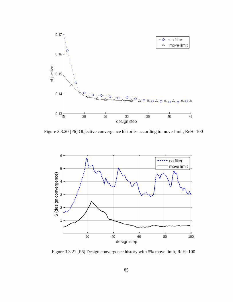
85

Figure 3.3.20 [P6] Objective convergence histories according to move-limit, ReH=100

Figure 3.3.21 [P6] Design convergence history with 5% move limit, ReH=100

20 40 60 80 100

1

2

3

4

5

6

design step

S (

de

sig

n c

on

ve

rge

nce

)

no filter

move limit

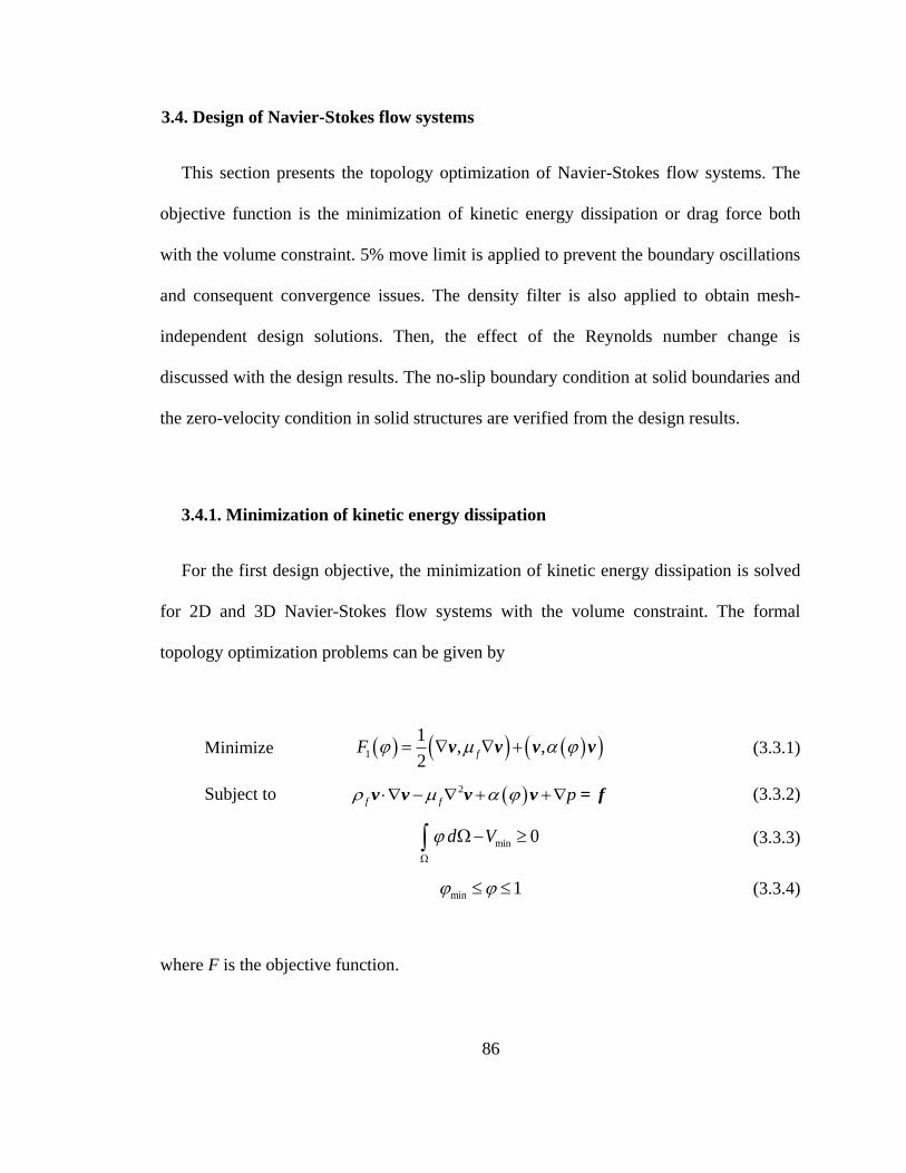
86

3.4. Design of Navier-Stokes flow systems

This section presents the topology optimization of Navier-Stokes flow systems. The

objective function is the minimization of kinetic energy dissipation or drag force both

with the volume constraint. 5% move limit is applied to prevent the boundary oscillations

and consequent convergence issues. The density filter is also applied to obtain mesh-

independent design solutions. Then, the effect of the Reynolds number change is

discussed with the design results. The no-slip boundary condition at solid boundaries and

the zero-velocity condition in solid structures are verified from the design results.

3.4.1. Minimization of kinetic energy dissipation

For the first design objective, the minimization of kinetic energy dissipation is solved

for 2D and 3D Navier-Stokes flow systems with the volume constraint. The formal

topology optimization problems can be given by

Minimize 1

1, ,

2fF v v v v (3.3.1)

Subject to 2

f f p v v v v = f (3.3.2)

min 0d V

(3.3.3)

min 1 (3.3.4)

where F is the objective function.

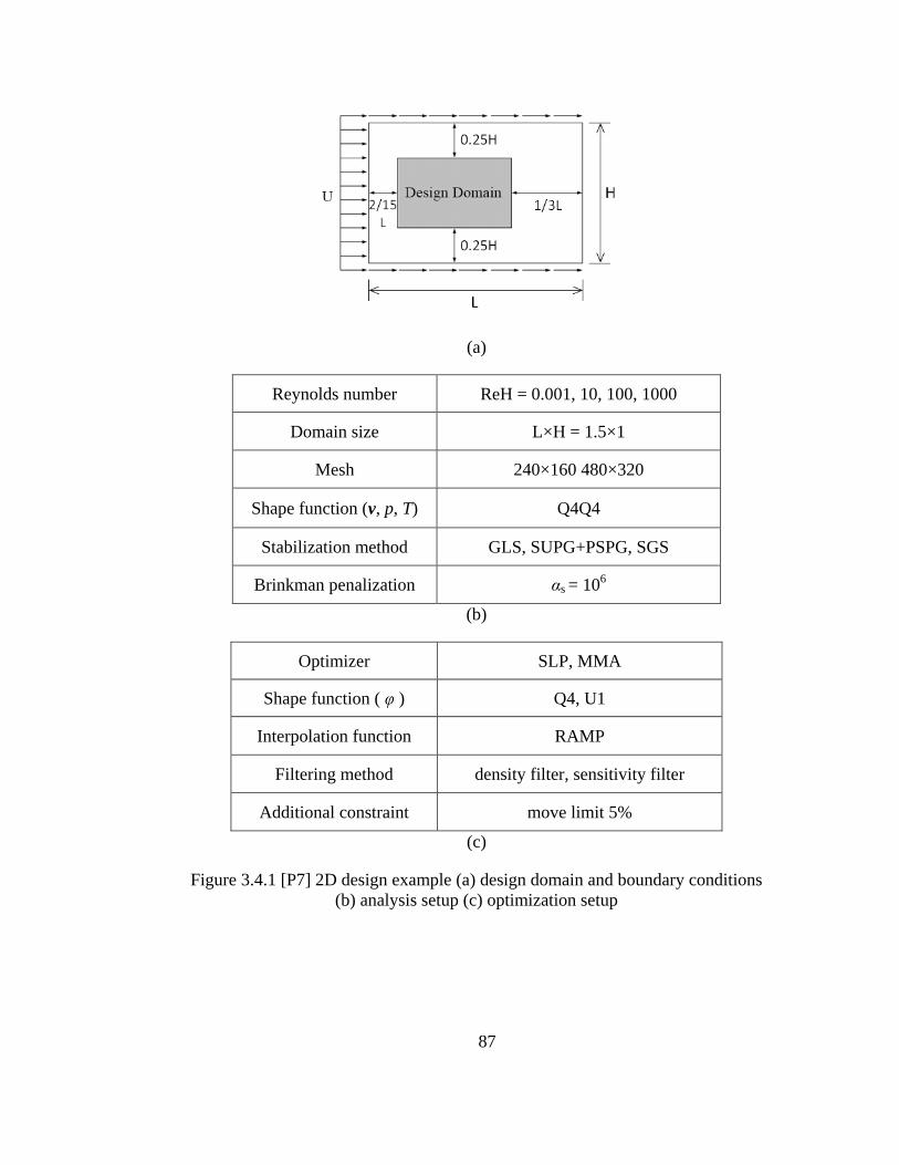
87

(a)

Reynolds number ReH = 0.001, 10, 100, 1000

Domain size L×H = 1.5×1

Mesh 240×160 480×320

Shape function (v, p, T) Q4Q4

Stabilization method GLS, SUPG+PSPG, SGS

Brinkman penalization αs = 106

(b)

Optimizer SLP, MMA



Filtering method density filter, sensitivity filter

Additional constraint move limit 5%

(c)



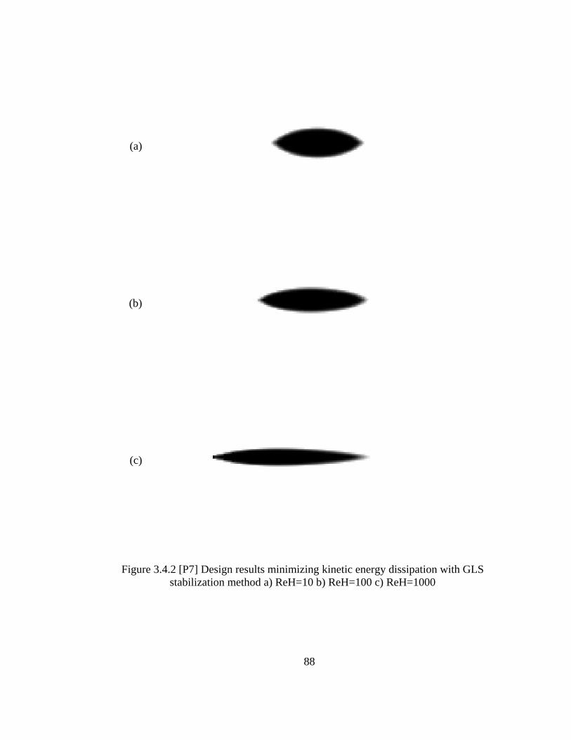
88

(a)

(b)

(c)

Figure 3.4.2 [P7] Design results minimizing kinetic energy dissipation with GLS

stabilization method a) ReH=10 b) ReH=100 c) ReH=1000

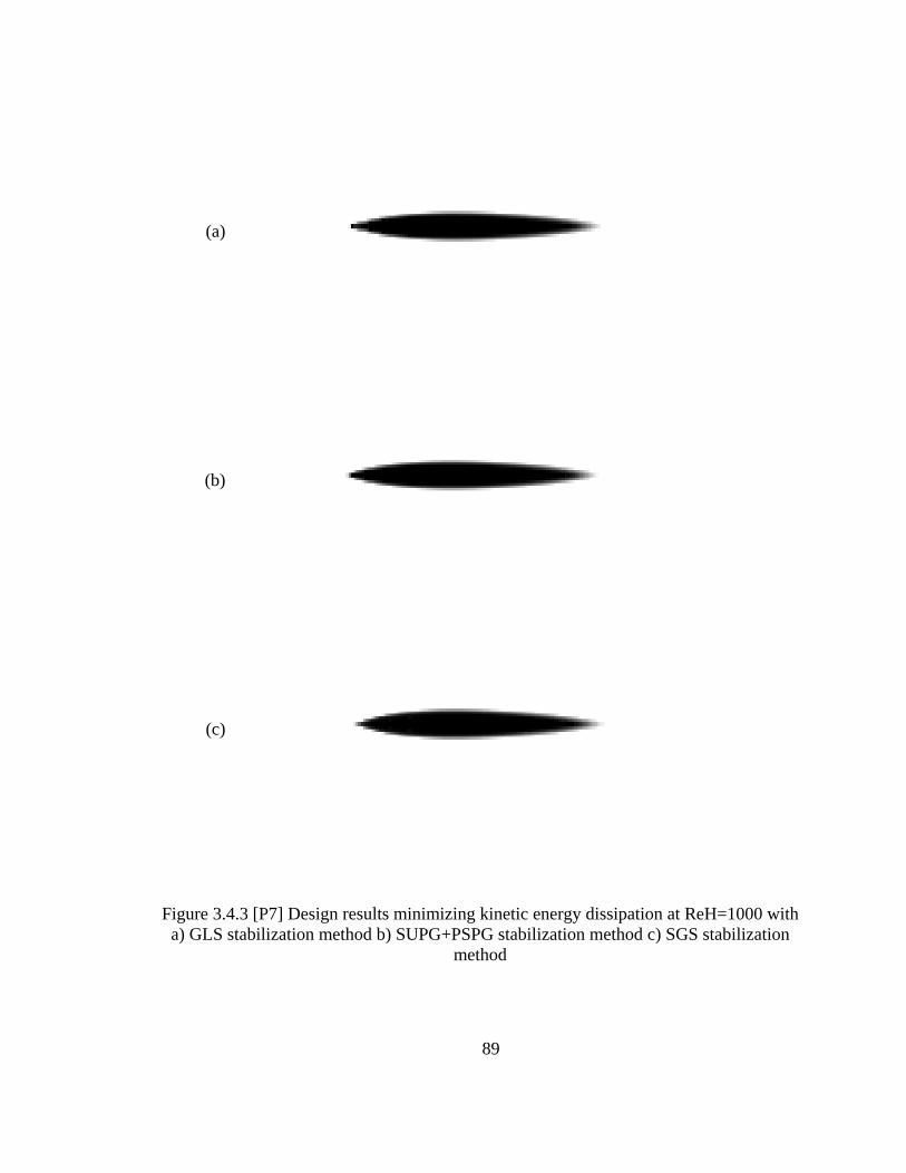
89

(a)

(b)

(c)

Figure 3.4.3 [P7] Design results minimizing kinetic energy dissipation at ReH=1000 with

a) GLS stabilization method b) SUPG+PSPG stabilization method c) SGS stabilization

method

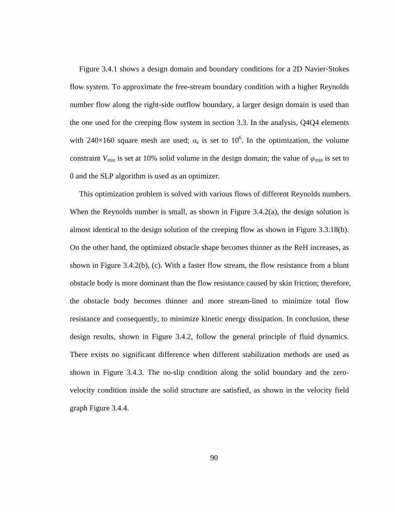
90

Figure 3.4.1 shows a design domain and boundary conditions for a 2D Navier-Stokes

flow system. To approximate the free-stream boundary condition with a higher Reynolds

number flow along the right-side outflow boundary, a larger design domain is used than

the one used for the creeping flow system in section 3.3. In the analysis, Q4Q4 elements

with 240×160 square mesh are used; αs is set to 106. In the optimization, the volume

constraint Vmin is set at 10% solid volume in the design domain; the value of φmin is set to

0 and the SLP algorithm is used as an optimizer.

This optimization problem is solved with various flows of different Reynolds numbers.

When the Reynolds number is small, as shown in Figure 3.4.2(a), the design solution is

almost identical to the design solution of the creeping flow as shown in Figure 3.3.18(b).

On the other hand, the optimized obstacle shape becomes thinner as the ReH increases, as

shown in Figure 3.4.2(b), (c). With a faster flow stream, the flow resistance from a blunt

obstacle body is more dominant than the flow resistance caused by skin friction; therefore,

the obstacle body becomes thinner and more stream-lined to minimize total flow

resistance and consequently, to minimize kinetic energy dissipation. In conclusion, these

design results, shown in Figure 3.4.2, follow the general principle of fluid dynamics.

There exists no significant difference when different stabilization methods are used as

shown in Figure 3.4.3. The no-slip condition along the solid boundary and the zero-

velocity condition inside the solid structure are satisfied, as shown in the velocity field

graph Figure 3.4.4.

91

(a)

(b) (c)

Figure 3.4.4 [P7] Design result and velotiy profiles at ReH=1000 (a) design result

(b) global velocity at section A-A' (c) local velocity view

-0.5 0 0.5 1 1.50

0.1

0.2

0.3

0.4

0.5

0.6

0.7

0.8

0.9

1

Vx at x=0.6

y

-4 -2 0 2 4

x 10-3

0.46

0.48

0.5

0.52

0.54

Vx at x=0.6

y

92

Finally, a 3D flow channel is designed following Aage’s study [51]. The design

domain and boundary conditions are shown in Figure 3.4.5. The Reynolds number is 100.

In the analysis, H8H8 elements with 40×40×40 cubic mesh are used with the GLS

stabilization method. In the optimization, the volume constraint Vmin is set at 50% solid

volume in the design domain. Figure 3.4.6 shows that the topology optimization method

creates a clear flow path inside the design domain, connecting one inlet with two outlets.

Figure 3.4.7 presents the objective and constraint converges very well.

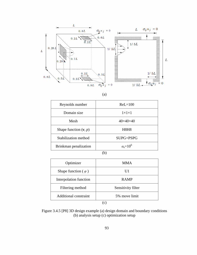
93

(a)

Reynolds number ReL=100

Domain size 1×1×1

Mesh 40×40×40

Shape function (v, p) H8H8

Stabilization method SUPG+PSPG

Brinkman penalization αs=106

(b)

Optimizer MMA

Shape function ( φ ) U1


Filtering method Sensitivity filter

Additional constraint 5% move limit

(c)



94

(a) (b)

Figure 3.4.6 [P8] Optimization results: (a) design result, (b) stream line graph

Figure 3.4.7 [P8] Convergence histories

0 5 10 15 20 25 30 35 400

0.1

0.2

0.3

0.4

0.5

0.6

0.7

0.8

0.9

1

design step

co

nve

rge

nce

objective F/Fo


95

3.5. Summary

In this chapter, the topology optimization of Navier-Stokes flow systems was

formulated. Relaxation schemes of discrete physical parameters such as the Brinkman

penalization parameter and the effective viscosity were revisited, and the adjoint

sensitivity method for a steady-state nonlinear system was described in detail. After

verifying the adjoint sensitivity method by comparing it with the finite difference

sensitivity, this topology optimization method was verified by comparing the results with

the previous topology optimization solutions of Stokes flow systems and the Pironneau’s

analytical solution [121].

I found numerical instabilities, such as element-scale cavities and boundary

oscillations, which prevent the design from converging. These numerical instabilities do

not result from an error in the sensitivity calculation or optimizer algorithms. Rather, they

are caused by the numerical instabilities at the system analysis level, which are discussed

in Section 2.5.2. Since the velocity and pressure oscillation becomes stronger as the

Reynolds number increases, these numerical instabilities at the optimization level become

more problematic with high Reynolds number flows.

Unlike the checkerboard problems of topology optimization, these numerical

instabilities, developed from element-scale cavities, are not successfully suppressed by

filtering schemes such as the density and sensitivity filter. This is mainly because the

locations of the cavities are not fixed through the design steps. The most effective and

easiest approach to prevent the instabilities is to apply a move limit. This constraint

96

successfully prevents the element-scale cavities and consequently suppresses boundary

oscillations without a significant increase in computational cost.

Finally, 2D and 3D flow channels were designed. The objective function was to

minimize kinetic power dissipation. The design solutions minimize skin friction with a

low Reynolds number flow while they minimize pressure drag, creating a thin

streamlined shape with a high Reynolds number flow.

97

CHAPTER 4

4. TOPOLOGY OPTIMIZATION OF CONVECTIVE COOLING SYSTEMS

4.1. Introduction

In accordance with the success of the topology optimization for Navier-Stokes flow

systems (chapter 3), the topology optimization method is also applied to convective heat

transfer problems in this chapter. For this multiphysics optimization, I analyze not only

heat transfers, but also flow motion without using the approximated side convection

coefficient ‘h.’ Therefore, this study extends previous topology optimization studies

considered single physics pure heat conduction problems [63-67] or quasi-multiphysics

heat transfer problems that use the side convection coefficient [68-70].

As explained in section 3.2, the discrete design variables are relaxed with continuous

interpolation functions, and then the adjoint sensitivities [114] are calculated. There are

two main differences between single physics fluid problems and these multiphysics

problems. First, an additional physical property is introduced to distinguish heat transfer

physics in free-fluid regions from those in solid regions. Second, the calculation of the

adjoint sensitivity for nonlinear multiphysics systems is much more complicated [114].

98

After presenting the procedure for calculating design sensitivity, additional numerical

instabilities, such as blocking wall designs resulting from unsuccessful Brinkman

penalization, are discovered and investigated. Several strategies are suggested for

preventing the blocking wall designs. Then, to validate the possibilities of the topology

optimization method in convective-cooling device designs, 2D and 3D design problems

with different Reynolds numbers and Prandtl numbers are presented and physically

interpreted.

The outline of this chapter is as follows. Section 4.2 presents the topology

optimization problems in convective heat transfer. Section 4.3 discusses numerical issues

and possible remedies. 2D and 3D design problems are presenting in section 4.4. Section

4.5 summarizes this chapter.

4.2. Sensitivity analysis for multiphysics problems

As indicated in section 3.2, the discrete design variables should be relaxed with

continuous interpolation functions, and the adjoint sensitivities should be calculated to

efficiently solve topology optimization problems. This section presents interpolation

functions used to relax the discrete design variables and explains how to calculate the

adjoint sensitivities for steady-state nonlinear multiphysics systems.

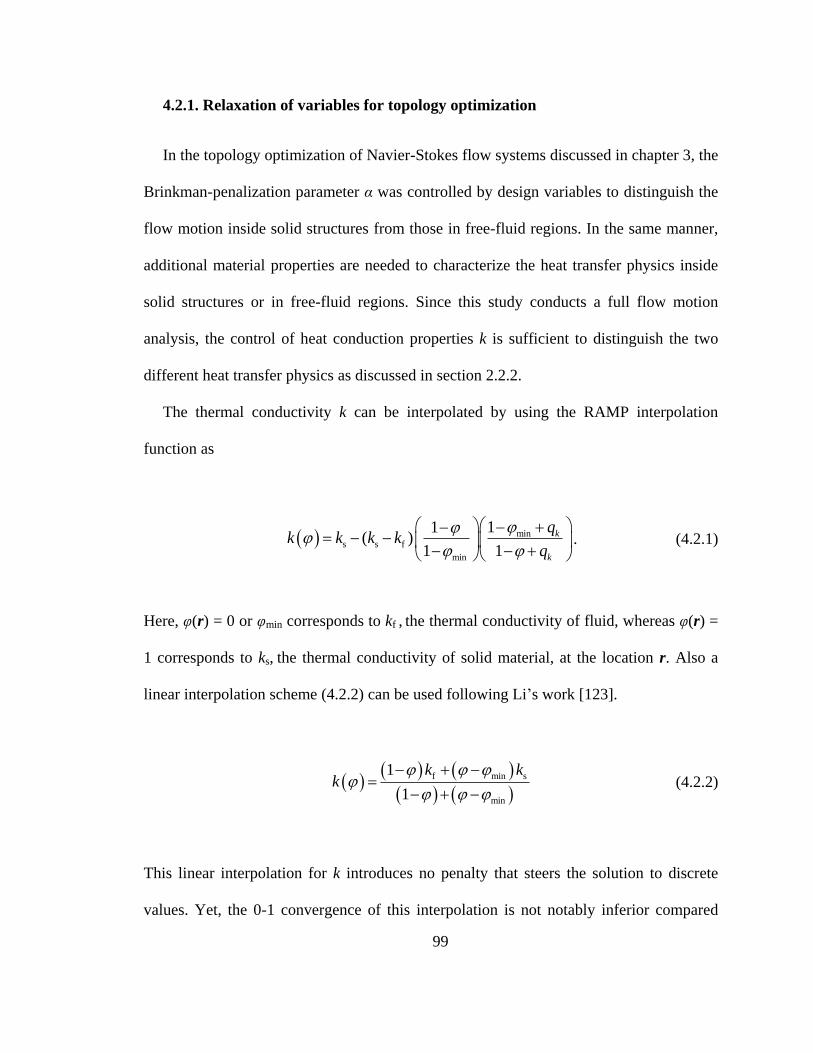
99

4.2.1. Relaxation of variables for topology optimization

In the topology optimization of Navier-Stokes flow systems discussed in chapter 3, the

Brinkman-penalization parameter α was controlled by design variables to distinguish the

flow motion inside solid structures from those in free-fluid regions. In the same manner,

additional material properties are needed to characterize the heat transfer physics inside

solid structures or in free-fluid regions. Since this study conducts a full flow motion

analysis, the control of heat conduction properties k is sufficient to distinguish the two

different heat transfer physics as discussed in section 2.2.2.

The thermal conductivity k can be interpolated by using the RAMP interpolation

function as

mins s f

min

11( )

1 1

k

k

qk k k k

q

. (4.2.1)

Here, φ(r) = 0 or φmin corresponds to kf , the thermal conductivity of fluid, whereas φ(r) =

1 corresponds to ks, the thermal conductivity of solid material, at the location r. Also a

linear interpolation scheme (4.2.2) can be used following Li’s work [123].

f min s

min

1

1

k kk

(4.2.2)

This linear interpolation for k introduces no penalty that steers the solution to discrete

values. Yet, the 0-1 convergence of this interpolation is not notably inferior compared

100

with that of RAMP interpolation probably because the RAMP interpolation for α already

has sufficient penalty effect. The relations between the design variable and the physics in

the free-fluid and solid regions becomes as shown in Table 4.2.1.

Table 4.2.1 Design variables and physical properties


Design variable φ(r) = 0, φmin φ(r) = 1


parameter α = αf ≈ 0 α = αs ≈ ∞

Heat conduction

coefficient k(φ) = kf k(φ) = ks

Momentum equation 2

f f p v v v = f 2

f p

v v = f

v 0

Energy equation 0f p fC T k T v

0sk T

Also, it should be noted that the RAMP interpolation scheme requires one more

heuristic control parameter qk, which makes it more difficult to control the already

complicated multiphysics optimization problem. Therefore, to simplify the optimization

problems, this study uses the same value for the control parameters qα and qk when

RAMP interpolation scheme is used to interpolate both the Brinkman penalization

parameter and the thermal conductivity.

101

4.2.2. Sensitivity analysis for multiphysics problems

Weakly coupled thermal-fluid equations (2.2.1) and (2.2.6) can be expressed in

residual form as

,U R u φ φ 0 (4.2.3)

, , ,T R T u φ u φ φ 0 . (4.2.4)

Here, UR and

TR is the residual form of the Brinkman-penalized Navier-Stokes equation

and homogenized heat transfer equation, respectively; both residual forms include the

stabilization terms. u is the fluid system response including velocity v and pressure p

while T is the heat transfer system response, temperature. Also cost functions and

constraints can be represented by the general response function F as

, , ,F Gφ T u φ u φ φ . (4.2.5)

Similarly to section 3.2.2, the dependence of the cost function F on the design vector φ

has been rewritten using the function G so as to isolate its implicit dependence on φ

through u(φ) and T(u, φ) from the explicit dependence on φ. Then the derivatives of the

response function with respect to the design variable becomes

i i i i

DF G D G D G

D D D

T u

T u (4.2.6)

102

The derivative DT/Dφi is an implicit quantity because the system response is implicitly

defined through equation (4.2.4).

T T T

i i i

D D

D D

R R RT u

T u. (4.2.7)

Then, by employing equation (3.1.7), DT/Dφi can be obtained as

1

U UT T T

i i i

D

D

R RR R RT

T u u. (4.2.8)

The direct differentiation sensitivities is calculated by

1

1 11

T T

i i i

U U UT T

i

DF G G

D

G G

R R

T T

R R RR R

T T u u u u

.

(4.2.9)

However, topology optimization problems generally have much more design variables φi

than response functions G, thus, this direct differentiation method is less efficient than the

adjoint sensitivity method as discussed in section 3.2.2.

To obtain adjoint sensitivity, an augmented functional is first defined as the

combination of equation (4.2.3), (4.2.4) and (4.2.5), given by

103

ˆ , , , ,

, , ,

U U

T T

F G

φ T u φ u φ φ λ φ R u φ φ

λ φ R T u φ u φ φ. (4.2.10)

Here, λU(φ) and λT(φ) are the Lagrange multipliers. Note that F F since UR and

TR are

zero vectors. Differentiation of the above with respect to the individual design parameters

φi yields

Û U

U

i i i i i i

T T TT

i i i

DF G G D G D D

D D D D

D D

D D

R Ru T uλ

u T u

R R Ru Tλ

u T.

(4.2.11)

To isolate the implicit response sensitivities, I separate equation (4.2.11) into three

terms

1 2

ˆ ˆˆÎ IE

i i i i

DF DFDFDF

D D D D (4.2.12)

where Ê iDF D is a explicit term and

1

Î iDF D and

2

Î iDF D are implicit terms,

respectively, defined as

ˆ

T TUE TU T

i i i i

DF G

D

R Rλ λ (4.2.13)

104

1

ˆ T T

I U TU T

i i

DF D G

D D

R Ruλ λ

u u u (4.2.14)

2

ˆ T

I TT

i i

DF D G

D D

RTλ

T T (4.2.15)

The implicit parts are eliminated from the sensitivity expression by defining the

Lagrange multipliers λU and λT so that equation (4.2.14) and equation (4.2.15) equal zero

as following

T

TT

G

Rλ

T T (4.2.16)

T T

U TU T

G

R Rλ λ

u u u.

(4.2.17)

Then, sensitivity expression reduces to the explicit terms of sensitivities as

ˆ

T TUE TU T

i i i i

DF G

D

R Rλ λ (4.2.18)

This adjoint sensitivities equation is basically the same as the direct differentiation

sensitivities equation (4.2.9). However, the number of response functional is generally

much small compared with the number of design parameters in topology optimization

problems. Therefore, it is more efficient to use the adjoint sensitivities than to use the

direct differentiation sensitivities [114].

105


This section presents a topology optimization example problem of thermal-fluid

systems and discusses numerical difficulties in the optimization process. Despite the

successful implementation of the topology optimization of Navier-Stokes flow systems,

the Brinkman-penalization does not work properly during the topology optimization of

multiphysics thermal-fluid systems, creating physically unacceptable design solutions.

This section discusses the reason for the numerical difficulties with numerical examples

and suggests possible solutions to circumvent the issues.

4.3.1. Unsuccessful Brinkman penalization and blocking wall designs

To clarify the numerical issue, this section considers an optimization problem of a 2D

cooling channel depicted in Figure 4.3.1. The design goal is set to minimize mean

temperature in the design domain. Parabolic flow profile with maximum flow velocity

Umax and uniform temperature T0 are given at the inlet boundary Γin. Zero pressure is

assumed at the outlet boundary Γout, without loss of generality. A uniform heat influx ‘h’

is applied at the heating boundary Γq. At the remaining wall boundary Γwall, no-slip

adiabatic boundary conditions are assumed. The material properties of antifreeze (50%)

and aluminum are used for the fluid material and the solid structure respectively. The

Reynolds number is first set to 10 and increased for later design, and the Prandtl number

of the fluid is 7.2.

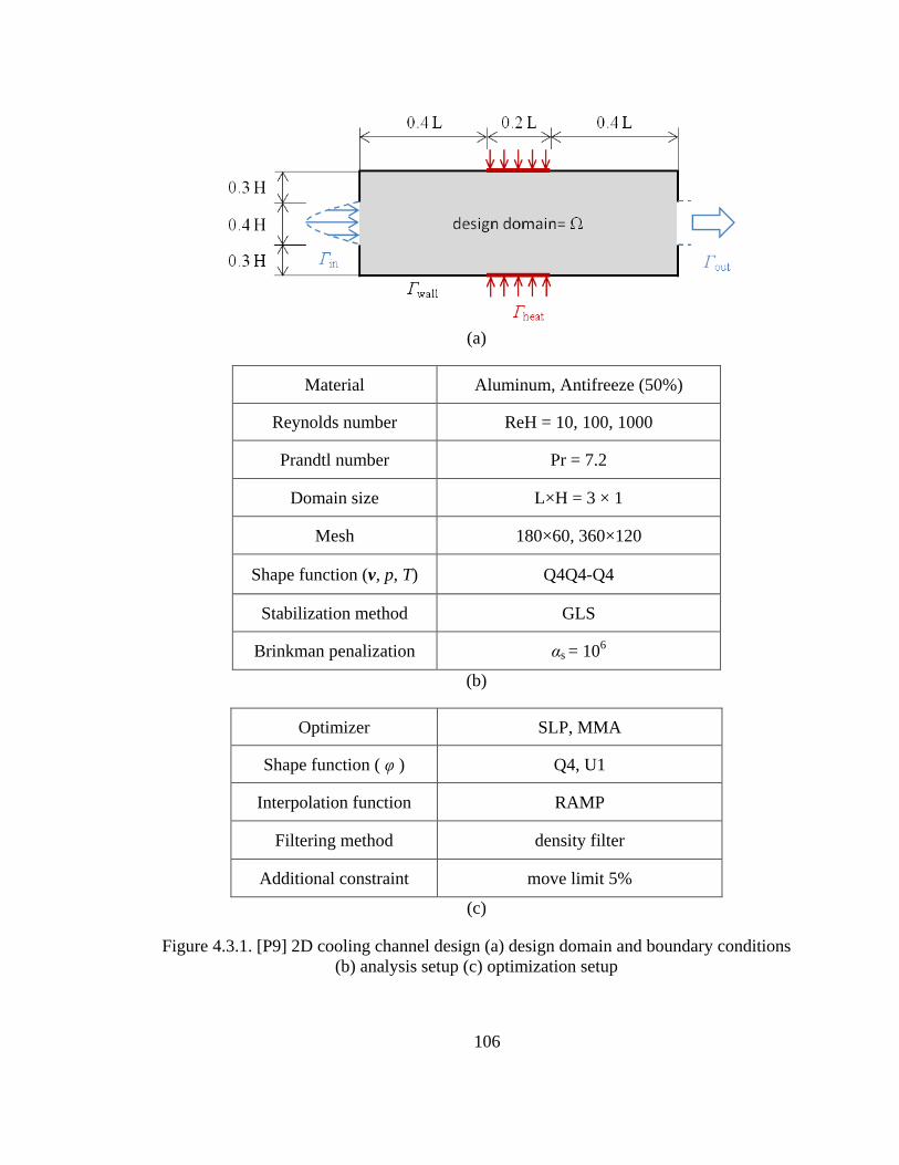
106

(a)

Material Aluminum, Antifreeze (50%)

Reynolds number ReH = 10, 100, 1000

Prandtl number Pr = 7.2

Domain size L×H = 3 × 1

Mesh 180×60, 360×120

Shape function (v, p, T) Q4Q4-Q4



(b)

Optimizer SLP, MMA



Filtering method density filter

Additional constraint move limit 5%

(c)

Figure 4.3.1. [P9] 2D cooling channel design (a) design domain and boundary conditions


107

The objective function and constraint function on the integral form are then defined

respectively as

Minimize 0

21

T T dF

d

(4.3.1)

Subject to 2

f f p v v v v = f (4.3.2)

0f pC T k T v (4.3.3)

*d V

(4.3.4)

0 1 (4.3.5)

The solid volume fraction V* is set to 0.2. The design variables are initially set to the

same value as the solid volume fraction V*.

Figure 4.3.2 shows the design result in case of Reh=10 and Reh=100, respectively.

With this design, the structure blocks flow path, and therefore no fluid can run through

the design domain in the real situation. However, this design results conflicts with the

continuity equation and the given boundary condition, and therefore the coolant

penetrates through the solid structures as shown in the streamline graph in Figure 4.3.2(c)

and Figure 4.3.2(e). Since the continuity equation and boundary conditions overrode

Brinkman penalization, the velocity was not penalized during FEM analysis and huge

computational error was observed. For example, when ReH = 100, the final objective

value Fo is only 13.3 according to the optimization result. However, if I cancel out the

impossible flow motion and consequent convective heat transfer inside the solid structure,

108

the correct mean temperature in the system becomes over 154. Figure 4.3.3 illustrates the

different temperature results. Since the Brinkman penalization did not enforce the zero

fluid velocity condition inside the solid structure, creating solid-penetrating coolant flow,

the temperature result, as shown Figure 4.3.3(d), becomes much better than the physically

correct temperature profile shown in Figure 4.3.3(c).

109

(a)

(b)

(c)

(d)

(e)

Figure 4.3.2. [P9] Design result of 2D cooling channel problems (a) design domain

(b) cooling channel design, ReH=10 (c) streamline graph, ReH=10

(d) cooling channel design, ReH=100 (e) streamline graph, ReH=100

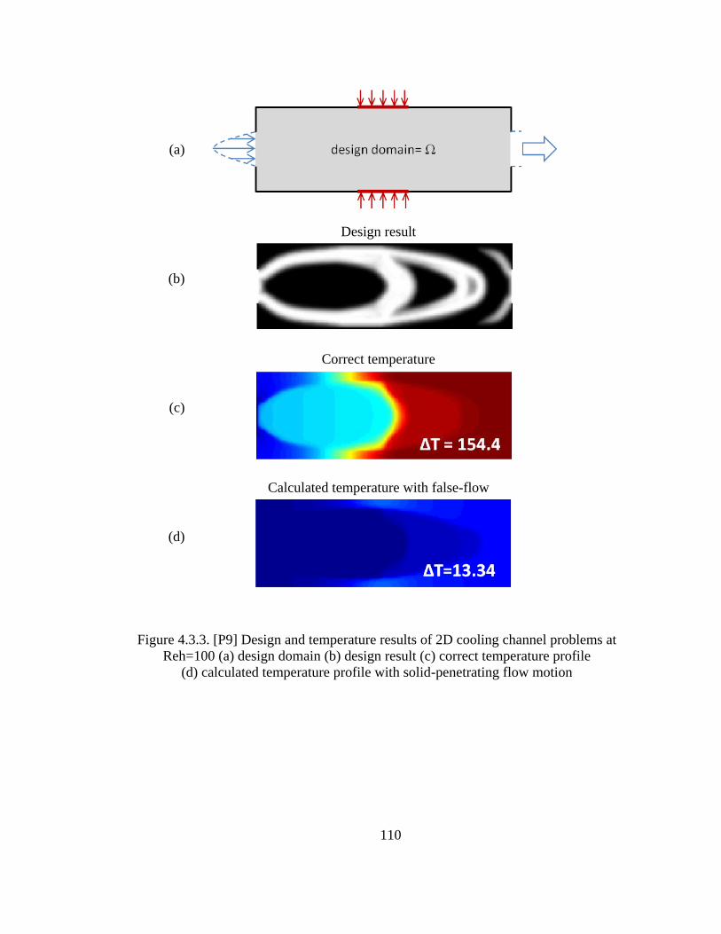
110

(a)

(b)

Design result

(c)

Correct temperature

(d)

Calculated temperature with false-flow

Figure 4.3.3. [P9] Design and temperature results of 2D cooling channel problems at

Reh=100 (a) design domain (b) design result (c) correct temperature profile

(d) calculated temperature profile with solid-penetrating flow motion

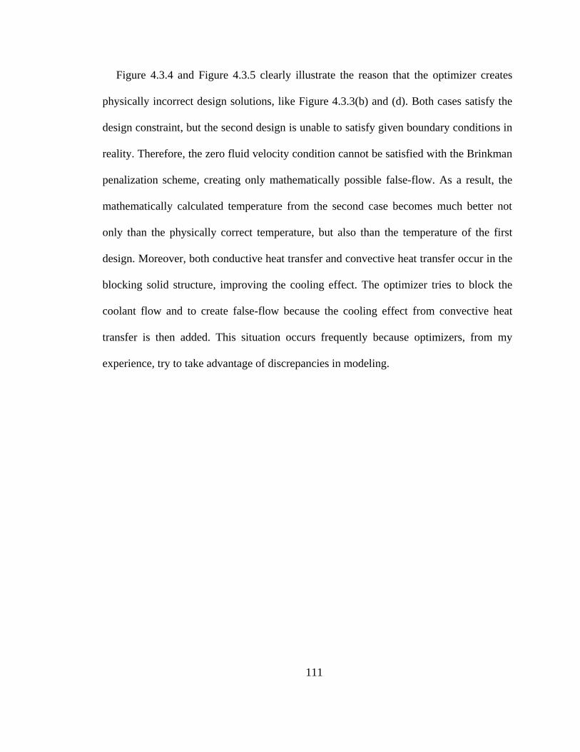
111

Figure 4.3.4 and Figure 4.3.5 clearly illustrate the reason that the optimizer creates

physically incorrect design solutions, like Figure 4.3.3(b) and (d). Both cases satisfy the

design constraint, but the second design is unable to satisfy given boundary conditions in

reality. Therefore, the zero fluid velocity condition cannot be satisfied with the Brinkman

penalization scheme, creating only mathematically possible false-flow. As a result, the

mathematically calculated temperature from the second case becomes much better not

only than the physically correct temperature, but also than the temperature of the first

design. Moreover, both conductive heat transfer and convective heat transfer occur in the

blocking solid structure, improving the cooling effect. The optimizer tries to block the

coolant flow and to create false-flow because the cooling effect from convective heat

transfer is then added. This situation occurs frequently because optimizers, from my

experience, try to take advantage of discrepancies in modeling.

112

(a)

Design example 1

(b)

Temperature profile T=30.9

Figure 4.3.4. [P9] Case 1: design and temperature results (a) design (b) temperature

(a)

Design example 2

(b)

Correct temperature profile T=2339

(c)

Calculated temperature with false-flow T=3.7

Figure 4.3.5. [P9] Case 2: design and temperature results (a) design (b) correct

temperature (c) calculated temperature profile with solid-penetrating flow motion

0

10

20

30

0

1000

2000

0

10

20

30

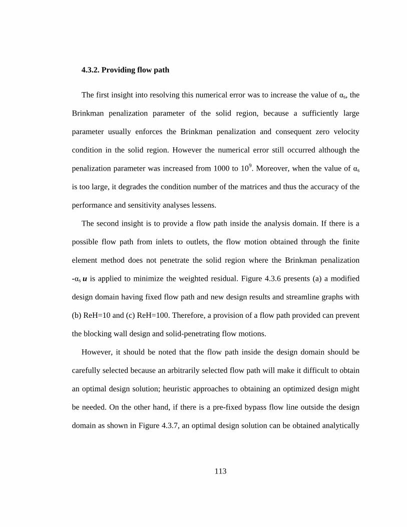
113

4.3.2. Providing flow path

The first insight into resolving this numerical error was to increase the value of αs, the

Brinkman penalization parameter of the solid region, because a sufficiently large

parameter usually enforces the Brinkman penalization and consequent zero velocity

condition in the solid region. However the numerical error still occurred although the

penalization parameter was increased from 1000 to 109. Moreover, when the value of αs

is too large, it degrades the condition number of the matrices and thus the accuracy of the

performance and sensitivity analyses lessens.

The second insight is to provide a flow path inside the analysis domain. If there is a

possible flow path from inlets to outlets, the flow motion obtained through the finite

element method does not penetrate the solid region where the Brinkman penalization

-αs u is applied to minimize the weighted residual. Figure 4.3.6 presents (a) a modified

design domain having fixed flow path and new design results and streamline graphs with

(b) ReH=10 and (c) ReH=100. Therefore, a provision of a flow path provided can prevent

the blocking wall design and solid-penetrating flow motions.

However, it should be noted that the flow path inside the design domain should be

carefully selected because an arbitrarily selected flow path will make it difficult to obtain

an optimal design solution; heuristic approaches to obtaining an optimized design might

be needed. On the other hand, if there is a pre-fixed bypass flow line outside the design

domain as shown in Figure 4.3.7, an optimal design solution can be obtained analytically

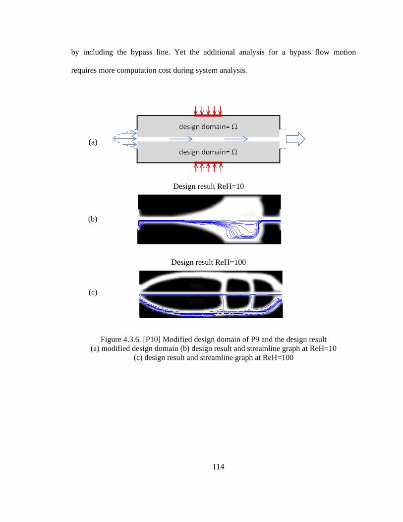
114

by including the bypass line. Yet the additional analysis for a bypass flow motion

requires more computation cost during system analysis.

(a)

(b)

Design result ReH=10

(c)

Design result ReH=100

Figure 4.3.6. [P10] Modified design domain of P9 and the design result

(a) modified design domain (b) design result and streamline graph at ReH=10

(c) design result and streamline graph at ReH=100

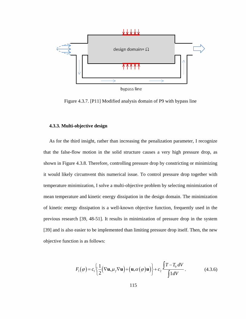
115

Figure 4.3.7. [P11] Modified analysis domain of P9 with bypass line

4.3.3. Multi-objective design

As for the third insight, rather than increasing the penalization parameter, I recognize

that the false-flow motion in the solid structure causes a very high pressure drop, as

shown in Figure 4.3.8. Therefore, controlling pressure drop by constricting or minimizing

it would likely circumvent this numerical issue. To control pressure drop together with

temperature minimization, I solve a multi-objective problem by selecting minimization of

mean temperature and kinetic energy dissipation in the design domain. The minimization

of kinetic energy dissipation is a well-known objective function, frequently used in the

previous research [39, 48-51]. It results in minimization of pressure drop in the system

[39] and is also easier to be implemented than limiting pressure drop itself. Then, the new

objective function is as follows:

0

1 1 2

1, ,

2 1f

T T dVF c c

dV

u u u u . (4.3.6)

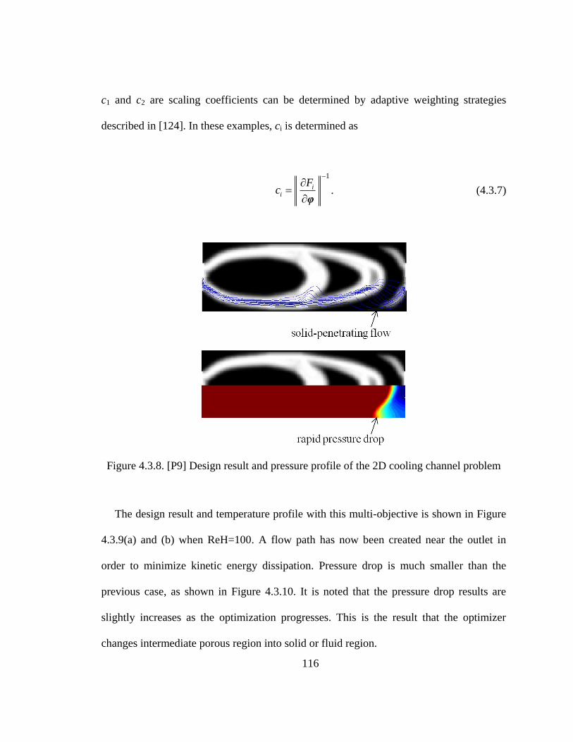
116

c1 and c2 are scaling coefficients can be determined by adaptive weighting strategies

described in [124]. In these examples, ci is determined as

1

ii

Fc

φ

. (4.3.7)

Figure 4.3.8. [P9] Design result and pressure profile of the 2D cooling channel problem

The design result and temperature profile with this multi-objective is shown in Figure

4.3.9(a) and (b) when ReH=100. A flow path has now been created near the outlet in

order to minimize kinetic energy dissipation. Pressure drop is much smaller than the

previous case, as shown in Figure 4.3.10. It is noted that the pressure drop results are

slightly increases as the optimization progresses. This is the result that the optimizer

changes intermediate porous region into solid or fluid region.

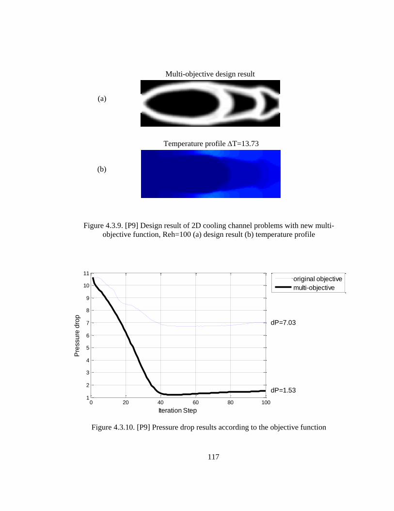
117

(a)

Multi-objective design result

(b)

Temperature profile T=13.73

Figure 4.3.9. [P9] Design result of 2D cooling channel problems with new multi-

objective function, Reh=100 (a) design result (b) temperature profile

Figure 4.3.10. [P9] Pressure drop results according to the objective function

0 20 40 60 80 1001

2

3

4

5

6

7

8

9

10

11

Pre

ssu

re d

rop

Iteration Step

original objective

multi-objective

dP=7.03

dP=1.53

118

The temperature profile of the new design is slightly worse than the previous design

result. However, if I compare it with the correct temperature result without false-flow

motion, the temperature profile of the new design is much better. Note that Figure 4.3.9(a)

shows two recirculation zones in the middle which should be avoided from a practical

standpoint. These recirculation zones occurred due to the volume constraint. If I increase

the solid volume in the design domain, the design results first fill out the recirculation

zone allowing the flow path to remain. It should be mentioned that this multi-objective

strategy should only be used for convection-dominated cases. For conduction-dominated

cases, their design results always try to create unnecessary flow paths, which lead to a

less effective cooling system structure.

4.4. Design of thermal-fluid cooling system

This section presents topology optimization problems of convective cooling systems.

The design goal is to minimize mean temperature in the design domain but, to prevent the

blocking wall design and solid-penetrating flow motion, multi-objective function

described in equation (4.3.6) is used. 5% move limit is applied to prevent the boundary

oscillations and consequent convergence issues. The density filter is also applied to

obtain mesh-independent design solution. Then, the effects of the Reynolds number and

Prandtl number change are discussed with design results.

119

4.4.1. 2D cooling channel designs

I designed 2D cooling channel previously depicted in Figure 4.3.1 by using the multi-

objective function, equation (4.3.6). The material properties of antifreeze and air, whose

Pr is 7.2 and 0.72 respectively, are used for the coolant with fixed inlet Reynolds

numbers from 10 to 1000. The material properties of aluminum are used for the solid

material. The solid volume fraction V* is set to 0.6 for all cases to observe the effect of

different Reh and Pr numbers. The design variables are initially set to the same value as

the solid volume fraction, V*. The mesh size is 360×120 and the degree of freedom is

approximately 1.75×105 in the fluid analysis. The number of design variables is 4.32×10

4.

When antifreeze (Pr=7.2) is used, it leads to the three different optimization results,

depending on the Reynolds number (Reh=10, 100, 1000) as presented in Figure 4.4.1. At

low speed flow, the solid region is attached to the two heating areas in the middle of the

top and bottom. However, as the Reynolds number is increased, the solid region is

detached from the heating areas and coolant flow directly impinges on the heat source.

With slower flow, the heat conduction effect becomes greater than the heat convection

effect, and therefore it is better to have solid structures functioning as cooling fins to

maximize the cooling effect by heat conduction. On the contrary, at higher Reynolds flow,

the cooling effect by heat convection becomes dominant and thus direct cooling is

preferable to attaching cooling fins to the heating area.

Figure 4.4.2 shows the optimization results when air is used for the coolant (Pr=0.72).

The cases of Reh=10, 100 and 1000 are tested in the same manner. Unlike the antifreeze

cases, the optimization results show similar structures in that aluminum is attached to

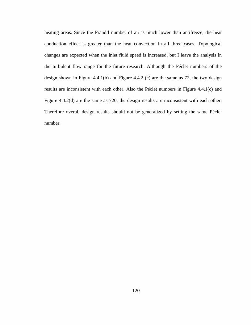
120

heating areas. Since the Prandtl number of air is much lower than antifreeze, the heat

conduction effect is greater than the heat convection in all three cases. Topological

changes are expected when the inlet fluid speed is increased, but I leave the analysis in

the turbulent flow range for the future research. Although the Péclet numbers of the

design shown in Figure 4.4.1(b) and Figure 4.4.2 (c) are the same as 72, the two design

results are inconsistent with each other. Also the Péclet numbers in Figure 4.4.1(c) and

Figure 4.4.2(d) are the same as 720, the design results are inconsistent with each other.

Therefore overall design results should not be generalized by setting the same Péclet

number.

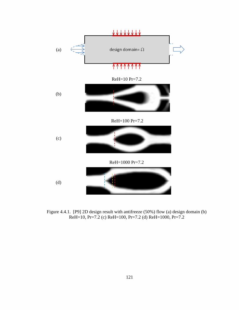
121

(a)

(b)

ReH=10 Pr=7.2

(c)

ReH=100 Pr=7.2

(d)

ReH=1000 Pr=7.2

Figure 4.4.1. [P9] 2D design result with antifreeze (50%) flow (a) design domain (b)

ReH=10, Pr=7.2 (c) ReH=100, Pr=7.2 (d) ReH=1000, Pr=7.2

122

(a)

(b)

ReH=10 Pr=0.72

(c)

ReH=100 Pr=0.72

(d)

ReH=1000 Pr=0.72

Figure 4.4.2. [P9] 2D design result with air flow (a) design domain (b) ReH=10, Pr=0.72

(c) ReH=100, Pr=0.72 (d) ReH=1000, Pr=0.72

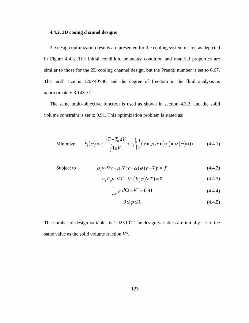
123

4.4.2. 3D cooing channel designs

3D design optimization results are presented for the cooling system design as depicted

in Figure 4.4.3. The initial condition, boundary condition and material properties are

similar to those for the 2D cooling channel design, but the Prandtl number is set to 6.67.

The mesh size is 120×40×40, and the degree of freedom in the fluid analysis is

approximately 8.14×105.

The same multi-objective function is used as shown in section 4.3.3, and the solid

volume constraint is set to 0.91. This optimization problem is stated as:

Minimize 0

1 1 2

1, ,

21f

T T dVF c c

dV

u u u u (4.4.1)

Subject to 2

f f p v v v v = f (4.4.2)

0f pC T k T v (4.4.3)

* 0.91d V

(4.4.4)

0 1 (4.4.5)

The number of design variables is 1.92×105. The design variables are initially set to the

same value as the solid volume fraction V*.

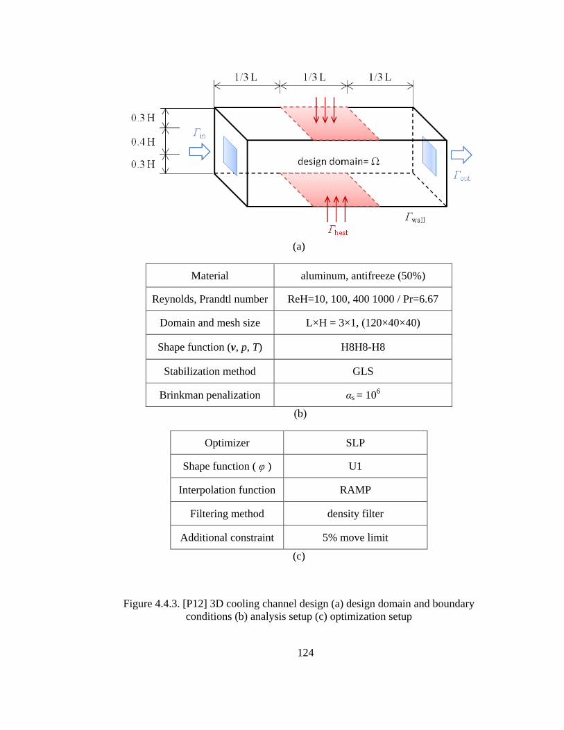
124

(a)

Material aluminum, antifreeze (50%)

Reynolds, Prandtl number ReH=10, 100, 400 1000 / Pr=6.67

Domain and mesh size L×H = 3×1, (120×40×40)

Shape function (v, p, T) H8H8-H8



(b)

Optimizer SLP

Shape function ( φ ) U1


Filtering method density filter

Additional constraint 5% move limit

(c)

Figure 4.4.3. [P12] 3D cooling channel design (a) design domain and boundary

conditions (b) analysis setup (c) optimization setup

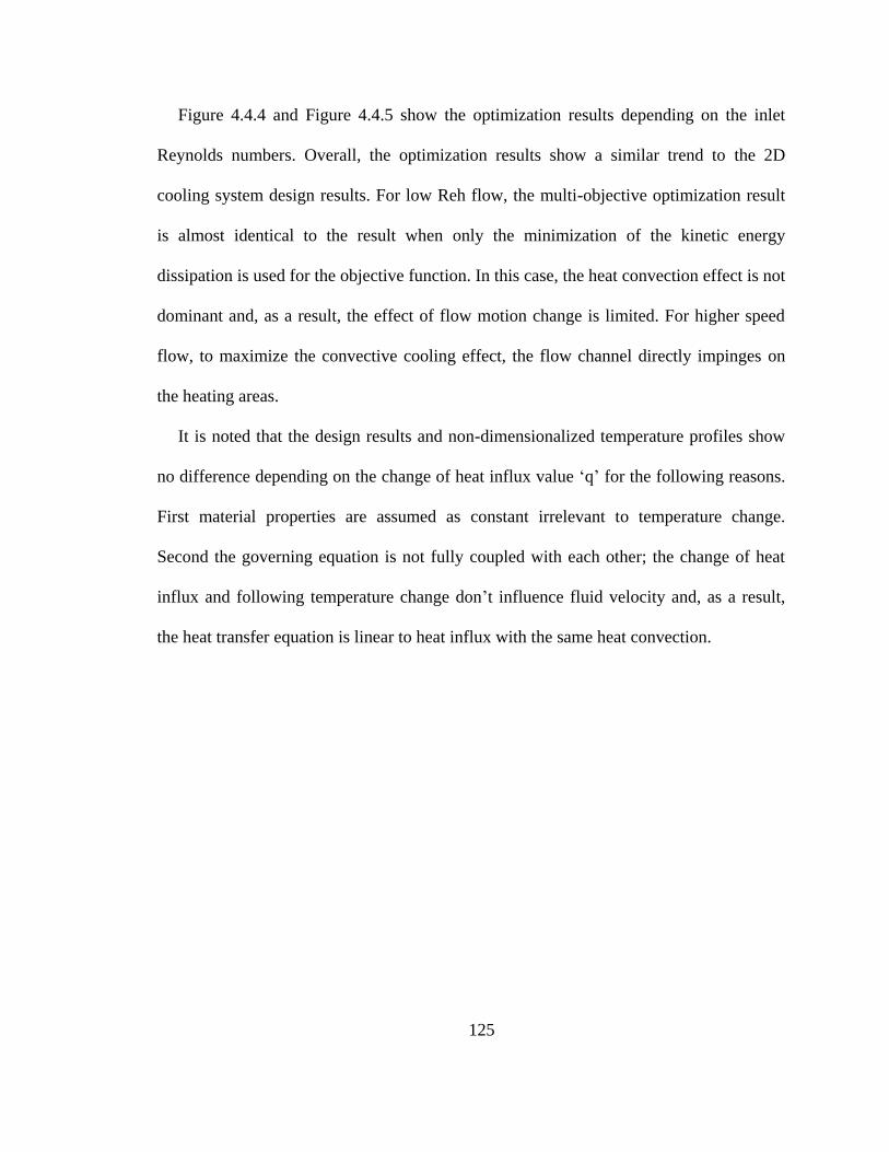
125

Figure 4.4.4 and Figure 4.4.5 show the optimization results depending on the inlet

Reynolds numbers. Overall, the optimization results show a similar trend to the 2D

cooling system design results. For low Reh flow, the multi-objective optimization result

is almost identical to the result when only the minimization of the kinetic energy

dissipation is used for the objective function. In this case, the heat convection effect is not

dominant and, as a result, the effect of flow motion change is limited. For higher speed

flow, to maximize the convective cooling effect, the flow channel directly impinges on

the heating areas.

It is noted that the design results and non-dimensionalized temperature profiles show

no difference depending on the change of heat influx value ‘q’ for the following reasons.

First material properties are assumed as constant irrelevant to temperature change.

Second the governing equation is not fully coupled with each other; the change of heat

influx and following temperature change don’t influence fluid velocity and, as a result,

the heat transfer equation is linear to heat influx with the same heat convection.

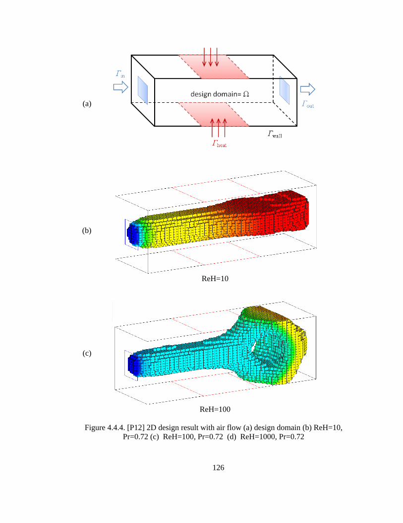
126

(a)

(b)

ReH=10

(c)

ReH=100


Pr=0.72 (c) ReH=100, Pr=0.72 (d) ReH=1000, Pr=0.72

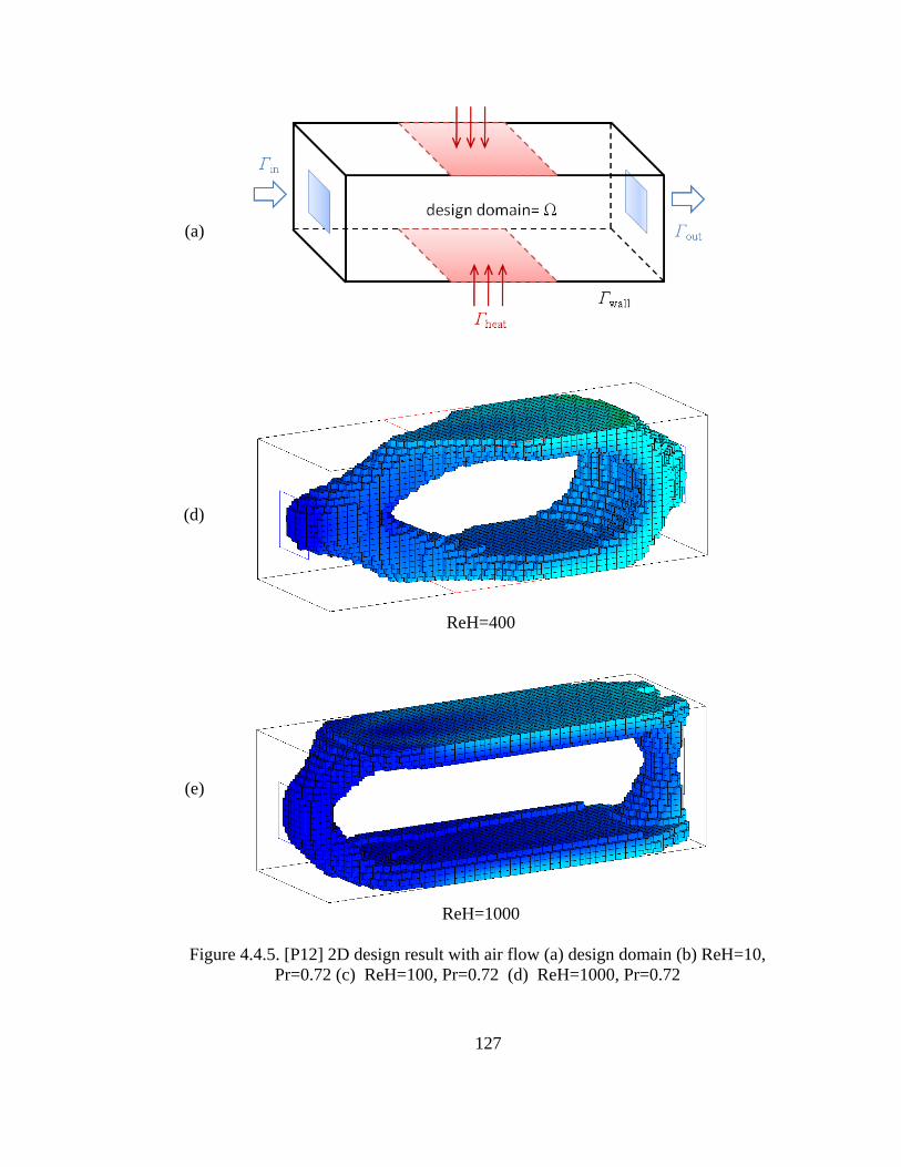
127

(a)

(d)

ReH=400

(e)

ReH=1000


Pr=0.72 (c) ReH=100, Pr=0.72 (d) ReH=1000, Pr=0.72

128

4.5. Summary

In this chapter, the topology optimization method of convective cooling systems was

presented. The main design purpose was to design a flow channel to minimize

temperature. After relaxation schemes of the thermal conductivity were revisited, the

adjoint sensitivity method for weakly coupled multiphysics systems was formulated,

extending the adjoint sensitivity formulation for steady-state nonlinear systems.

The Brinkman penalization, which is successfully applied to the topology optimization

of single physics Navier-Stokes flow systems as shown in chapter 3, fails to enforce the

zero-velocity condition inside solid structures and the no-slip boundary condition at solid

surfaces. This happens when the design results block all possible coolant flow paths.

Such designs conflict with the principle of mass conservation and given boundary

conditions. As a result, the mass conservation law and given boundary conditions

override the Brinkman penalization, creating solid-penetrating false flow. Since the

mathematically calculated cooling effect with the false flow is usually superior,

optimizers prefer to design the blocking walls ignoring the Brinkman penalization.

If a fixed flow path from inlets to outlets is given, there is no possible conflict between

the design and the physical laws. Thus, the topology optimization method produces

physically correct design results. Therefore, providing a fixed-flow path inside or outside

of the design domains resolves this numerical issue. However, the flow path inside the

design domain is heuristically given, and the flow path outside the design domain

increases computational cost.

129

Mathematically, the false flow generates a high pressure drop when it penetrates solid

structures. Therefore, a multi-objective function to minimize both the pressure drop and

temperature was implemented to circumvent the numerical issue and successfully

produces physically acceptable optimization results. Implementing the multi-objective

function enabled the solution of example problems of 2D and 3D convective cooling

systems, and the effect of Reynolds number and Prandtl number changes were explored.

130

CHAPTER 5

5. CONCLUSION

5.1. Concluding remarks

This dissertation investigates the topology optimization of convective cooling systems,

extending previous topology optimization research of Stokes flow systems and heat

conduction systems. The flow analysis results are used to solve the thermal transport

equation without using the heat convection coefficient. For accurate and cost-effective

analysis, the stabilized finite element methods and the adjoint sensitivity for weakly

coupled multiphysics systems are implemented. Numerical instabilities are presented and

discussed at the system analysis and design optimization levels. 2D and 3D flow channels

are designed as design examples to minimize the kinetic energy dissipation or to

minimize the temperature in the system.

Thermal-fluid analysis for topology optimization

This study introduces a fictitious domain approach, which uses an immersed

boundaries concept, Brinkman penalization and the homogenized property of thermal

131

conductivity. By implementing this analysis method, this study extends the region

topology optimization from linear Stokes flow and heat conduction systems to convective

cooling systems that are nonlinear coupled multiphysics systems. A guideline for setting

a proper lower bound of the Brinkman penalization parameter is presented. When the

Brinkman penalization parameter is greater than 106 (Da=10

-6), the zero-velocity

condition in solid regions and the no-slip boundary condition at solid boundaries are

satisfied. To establish a stable and cost-effective method, various stabilized finite element

methods are examined, and the Newton-Raphson method is used with a simultaneous

stabilization tensor update scheme and Reynolds-Ramping initial guess strategy.

Numerical issues such as velocity and pressure oscillations are presented.

These numerical instabilities occur because the velocity gradient changes too sharply

at the fluid-solid interfaces for the stabilized finite element solution to correctly capture

the velocity profile. The oscillation becomes severe when the Reynolds number increases.

Although mesh refinement can smooth this oscillation, it is not viable because it increases

the computation cost of the topology optimization. The GLS stabilization method

produces the weakest oscillation, but the difference in solutions produced by different

stabilization tensors is not significant.

Topology optimization of Navier-Stokes flow systems

The topology optimization of Navier-Stokes flow systems is investigated, extending

previous topology optimization researches of Stokes flow systems to nonlinear Navier-

Stokes flow system. The adjoint sensitivity method is implemented, and relaxation

schemes used in previous topology optimization of Stokes flow systems are revised.

132

Element-scale cavities and consequent boundary oscillation phenomenon, which prevent

design convergence, are presented and investigated. These numerical instabilities result

from the numerical issues in the system analysis such as pressure oscillation at the

immersed boundaries. A move-limit successfully suppresses the numerical instabilities

while the density filter, the sensitivity filter and higher interpolation functions for design

variables are not effective. Using this approach, I present 2D and 3D design problems and

interpret the physics in the design solutions. The objective function is the minimization of

kinetic energy dissipation or drag minimization. The design solutions minimize skin

friction with a low Reynolds number while minimizing pressure drag, creating a thin

streamlined shape with a high Reynolds number.

Topology optimization of convective cooling systems

The topology optimization of convective cooling systems is investigated, extending

and combining previous topology optimization research of Navier-Stokes flow systems

and heat conduction systems. The main design purpose is to design a flow channel to

maximize cooling efficiency. The adjoint sensitivity method is formulated for nonlinear

multiphysics problems, and relaxation schemes used in previous topology optimization

are revised. The optimizer frequently tries to produce physically impossible design results

that have a conflict between the Brinkman penalization from the mass conservation law

and given boundary conditions. This is because the mathematically calculated cooling

effect is superior given this conflict. However, in reality, no coolant flow can run through

the system designed, so the temperature is very high. This numerical issue can be

circumvented by providing a fixed-flow path or by solving a multi-objective function that

133

minimizes both temperature and pressure drop. Finally, by implementing the multi-

objective function, example problems of 2D and 3D convective cooling systems are

solved and the effect of Reynolds number and Prandtl number changes are discussed.

5.2. Future works

Following are some of the interesting directions to which this research can be

extended.

Implementing fully coupled physical properties

This dissertation reviewed the thermal-fluid analysis method, which includes the

Brinkman-penalized Navier-Stokes equation (2.2.3) and the homogenized thermal

transport equation (2.2.6). In the momentum equation, the material properties relating to

temperature are assumed as constants, so as to decouple temperature and enable cost

effective analysis. However, the material properties, such as fluid density and viscosity

should be assumed as functions of temperature instead of constants in order to obtain

accurate solutions when the temperature varies significantly. In such cases, the velocity,

pressure and temperature profiles should be calculated simultaneously, while this study

solves the momentum equation and the energy equation sequentially. An analysis of the

differences between the optimum shapes obtained under different conditions of the

physical properties would be a valuable contribution.

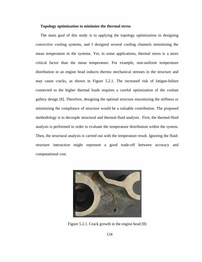
134

Topology optimization to minimize the thermal stress

The main goal of this study is to applying the topology optimization in designing

convective cooling systems, and I designed several cooling channels minimizing the

mean temperature in the systems. Yet, in some applications, thermal stress is a more

critical factor than the mean temperature. For example, non-uniform temperature

distribution in an engine head induces thermo mechanical stresses in the structure and

may cause cracks, as shown in Figure 5.2.1. The increased risk of fatigue-failure

connected to the higher thermal loads requires a careful optimization of the coolant

gallery design [8]. Therefore, designing the optimal structure maximizing the stiffness or

minimizing the compliance of structure would be a valuable contribution. The proposed

methodology is to decouple structural and thermal-fluid analysis. First, the thermal-fluid

analysis is performed in order to evaluate the temperature distribution within the system.

Then, the structural analysis is carried out with the temperature result. Ignoring the fluid-

structure interaction might represent a good trade-off between accuracy and

computational cost.

Figure 5.2.1. Crack growth in the engine head [8]

135

Adding the effect of the viscous dissipation

From practical standpoint, the present work neglects the effect of the viscous

dissipation term on heat transfer. Although this computational model is expected to be

reasonably accurate for most applications, this viscous dissipation term can be important

when the viscosity and velocity gradients are high. Furthermore, the multi-objective

function (4.4.1), used to resolve the blocking wall design, includes the kinetic dissipation

terms. Therefore, an investigation of the alterations induced by viscous dissipation in the

optimum channel shape would enhance our understanding.

136

APPENDIX

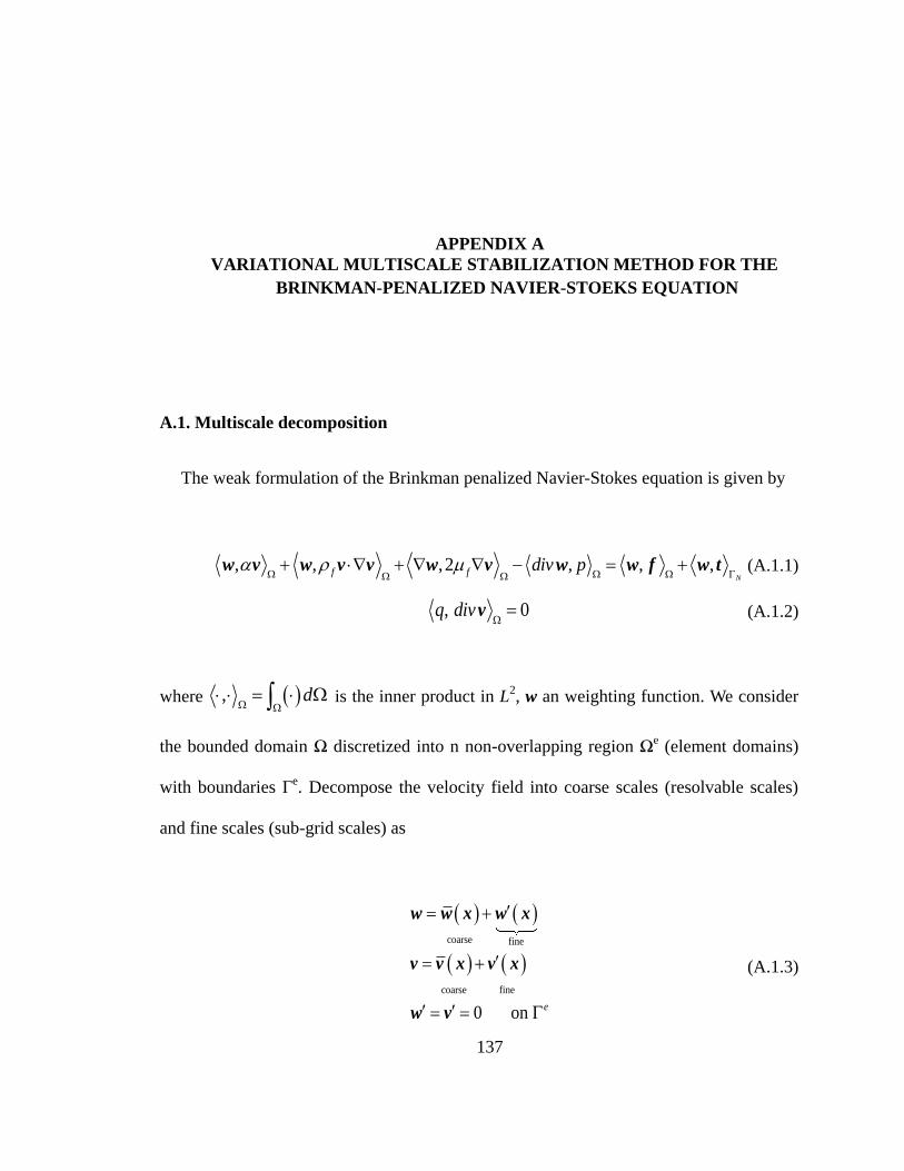
137

APPENDIX A

A.VARIATIONAL MULTISCALE STABILIZATION METHOD FOR THE

BRINKMAN-PENALIZED NAVIER-STOEKS EQUATION

A.1. Multiscale decomposition

The weak formulation of the Brinkman penalized Navier-Stokes equation is given by

, , ,2 , , ,N

f f div p w v w v v w v w w f w t (A.1.1)

, 0q divv (A.1.2)

where , d

is the inner product in L2, w an weighting function. We consider

the bounded domain Ω discretized into n non-overlapping region Ωe (element domains)

with boundaries Гe. Decompose the velocity field into coarse scales (resolvable scales)

and fine scales (sub-grid scales) as

coarse fine

coarse fine

0 on e

w w x w x

v v x v x

w v

(A.1.3)

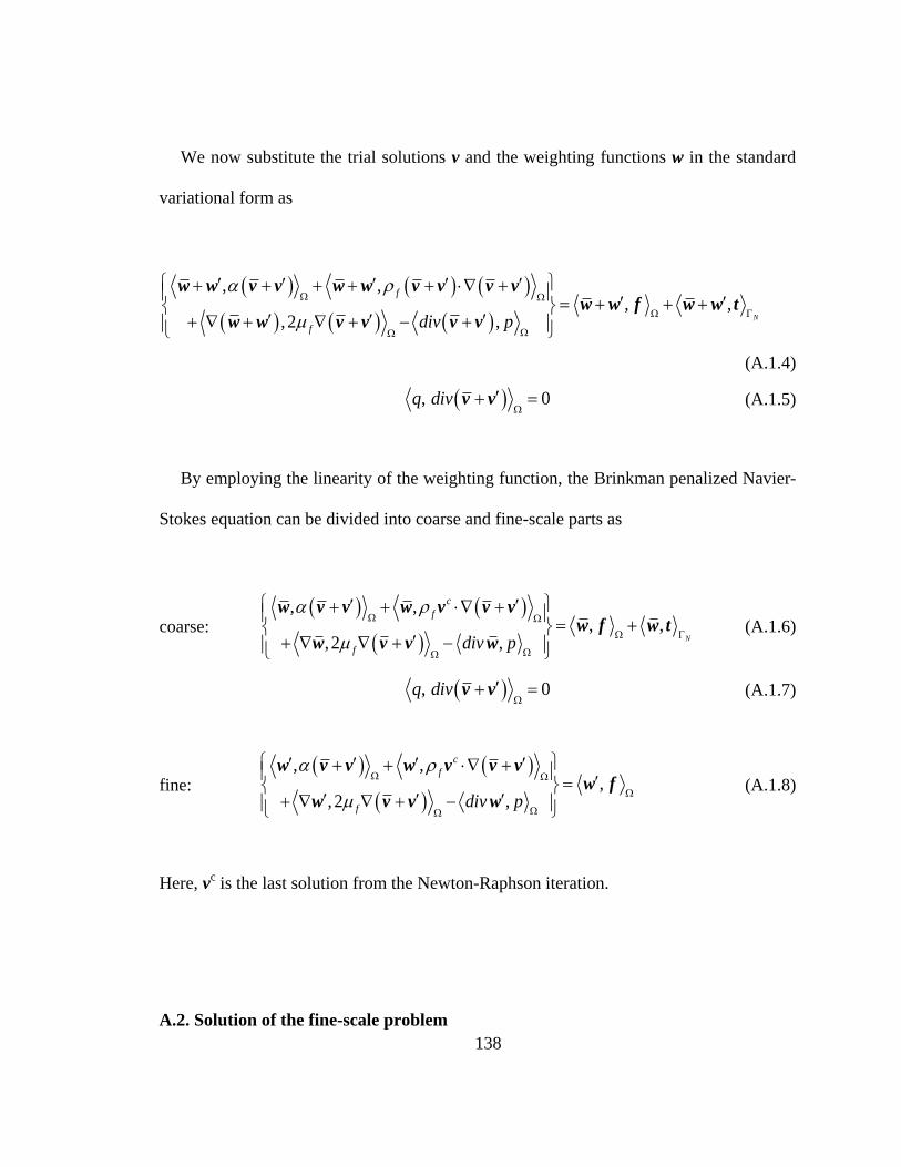
138

We now substitute the trial solutions v and the weighting functions w in the standard

variational form as

, ,, ,

, 2 , N

f

f div p

w w v v w w v v v vw w f w w t

w w v v v v

(A.1.4)

, 0q div

v v (A.1.5)

By employing the linearity of the weighting function, the Brinkman penalized Navier-

Stokes equation can be divided into coarse and fine-scale parts as

coarse:

, ,, ,

, 2 , N

c

f

f div p

w v v w v v vw f w t

w v v w (A.1.6)

, 0q div

v v (A.1.7)

fine:

, ,,

, 2 ,

c

f

f div p

w v v w v v vw f

w v v w (A.1.8)

Here, vc is the last solution from the Newton-Raphson iteration.

A.2. Solution of the fine-scale problem

139

Rearrange fine-scale equation as

, , , 2

, , , , , 2

c

f f

c

f fp

w v w v v w v

w f w w v w v v w v

, 2 ,c

f fp

w f v v v v w r (A.2.1)

where 2c

f fp r f v v v v . Assume the fine scale v′ and w′ are

represented via bubble functions as

1

2

| ,

|

e

e

e

i i

e

i i

b

b

v β

w γ (A.2.2)

Then, the equation becomes:

2 1 2 1

2

2 1 2 1

e e

e

e e

e e e e c e e

fT T e e

e e e e e e

f f

b b d b b db d

b b d b b d

I v Iγ β γ r

I (A.2.3)

Because β is arbitrary, we have

1β K R (A.2.4)

Here,

140

2 1 2 1

2 1 2 1

e e

e e

e e e e c e e

f

e e e e e e

f f

b b d b b d

b b d b b d

K I v I

I (A.2.5)

2e

e eb d

R r (A.2.6)

We now reconstruct the fine-scale filed over the element domain as

1

1 1

e eb b v β K R (A.2.7)

A.3. Solution of the coarse-scale problem with incompressible constraint

The coarse-scale problem (A.1.5) can be written as

, , 0q div q

v v. (A.3.1)

Substitute v′ from (A.2.7) to get

1

1, , 0eq div q b

v K R . (A.3.2)

Consider the second term on the left-hand side of (A.3.2)

141

1

1

1

1 2

, ,

,e

e

e e e

V

q q b

q b b dV

v K R

K r

,q

τr. (A.3.3)

Here,

1

2 1 2 1

1 2

2 1 2 1

e e

e

e e

e e e e c e e

fe e e V V

e e e e e eVf f

V V

b b dV b b dVb b dV

b b dV b b dV

I v Iτ

I . (A.3.4)

Consequently, the coarse-scale equation (A.3.1) becomes

, , 2 ,c

f fq div q p q v τ v v v v f τf

. (A.3.5)

Now, extract the fine-scale velocity field from coarse-scale equation (A.1.6) as

, , , 2 ,, ,

, , , 2 N

c

f f

c

f f

div p

w u w v v w v ww f w t

w v w v v w v.

(A.3.6)

Applying integration by pars as

, , ,c c c

f f

w v v w v n v v w v (A.3.7)

,2 ,2 ,2f f f

w v w v w v (A.3.8)

142

Then the equation becomes

, , , 2 ,, ,

, , , 2 N

c

f f

c

f

div p

w v w v v w v ww f w t

w v v w v w v

(A.3.9)

Substitute v’

, , , 2

2 ,

2 , 2

c

f

c

f

c c

f f f p

w v v w v w v

w v w w v

w v w w τ f u v v v

(A.3.10)

The weak form of the momentum equation finally becomes

, , , 2 ,

2 , 2

, , 2 ,N

c

f f

c c

f f f

c

f

div p

p

w u w v v w v w

w v w w τ v v v v

w f w t w v w w τf

(A.3.11)

Here, the stabilization tensor is given by (A.3.4).

143

BIBLIOGRAPHY

144

[1] M. P. Bendsøe and N. Kikuchi, "Generating Optimal Topologies in Structural

Design Using a Homogenization Method," Computer Methods in Applied

Mechanics and Engineering, vol. 71, pp. 197-224, 1988.

[2] G. H. Kim, et al., Battery thermal management system design modeling: National

Renewable Energy Laboratory, 2006.

[3] S. Al-Hallaj and J. Selman, "Thermal modeling of secondary lithium batteries for

electric vehicle/hybrid electric vehicle applications," Journal of power sources,

vol. 110, pp. 341-348, 2002.

[4] K. Shukuya, et al., "A New Battery System for the Estima Hybrid Minivan," 2002.

[5] M. G. Gavali, et al., "Optimization of Water Jacket Using CFD for Effective

Cooling of Water-Cooled Diesel Engines," presented at the Symposium on

International Automotive Technology, 2007.

[6] S. Shih, et al., "Engine knock toughness improvement through water jacket

optimization," presented at the Powertrain & Fluid Systems Conference &

Exhibition, 2003.

[7] J. Ye, et al., "Coolant Flow Optimization in a Racing Cylinder Block and Head

Using Cfd Analysis and Testing," in Motorsports Engineering Conference &

Exposition, 400 Commonwealth Dr , Warrendale, PA, 15096, USA, 2004.

[8] G. Cantore, et al., "Optimization of a cooling circuit in an internal combustion

engine for marine applications," presented at the Internation Conference on

Engines for Automobile, 2005.

[9] N. León, et al., "Automatic shape variations for optimization and innovation,

Shape Optimization of Cylinderhead Gasket using CFD," IFIP International

Federation for Information Processing, vol. 250, p. 179, 2007.

[10] F. Farina, et al., "Thermal design of integrated motor drives for traction

applications," in Power Electronics and Applications, 2005 European Conference

on, 2005, pp. 10 pp.-P.10.

145

[11] Z. Ping, et al., "Research on the Cooling System of a 4QT Prototype Machine

Used for HEV," Energy Conversion, IEEE Transactions on, vol. 23, pp. 61-67,

2008.

[12] I. Khorunzhii, et al., "Modelling of a pin-fin heat converter with fluid cooling for

power semiconductor modules," International Journal of Energy Research, vol.

27, pp. 1015-1026, 2003.

[13] K. Park, et al., "Numerical shape optimization for high performance of a heat sink

with pin-fins," Numerical Heat Transfer Part A: Applications, vol. 46, pp. 909-

927, 2004.

[14] Y.-T. Yang and H.-S. Peng, "Numerical study of pin-fin heat sink with un-

uniform fin height design," International Journal of Heat and Mass Transfer, vol.

51, pp. 4788-4796, 2008.

[15] Y.-T. Yang and H.-S. Peng, "Numerical study of the heat sink with un-uniform

fin width designs," International Journal of Heat and Mass Transfer, vol. 52, pp.

3473-3480, 2009.

[16] K.-S. Lee, et al., "Optimal shape and arrangement of staggered pins in the channel

of a plate heat exchanger," International Journal of Heat and Mass Transfer, vol.

44, pp. 3223-3231, 2001.

[17] K. Park and D.-H. Choi, "Shape Optimization of a plate-fin type heat sink with

triangular-shaped vortex generator," Journal of Mechanical Science and

Technology, vol. 18, pp. 1590-1603, 2004.

[18] K. Park, et al., "The application of the CFD and Kriging method to an

optimization of heat sink," International Journal of Heat and Mass Transfer, vol.

49, pp. 3439-3447, 2006.

[19] A. Husain and K. Kwang-Yong, "Shape Optimization of Micro-Channel Heat

Sink for Micro-Electronic Cooling," Components and Packaging Technologies,

IEEE Transactions on, vol. 31, pp. 322-330, 2008.

[20] C. Silva, et al., "Optimization of Fin Performance in a Laminar Channel Flow

Through Dimpled Surfaces," Journal of Heat Transfer, vol. 131, pp. 021702-9,

2009.

146

[21] A. Samad, et al., "Multi-objective optimization of a dimpled channel for heat

transfer augmentation," Heat and Mass Transfer, vol. 45, pp. 207-217, 2008.

[22] D. Kuhl, et al., "Structural optimization of rocket engine cooling channels,"

presented at the AIAA/ASME/SAE/ASEE Joint Propulsion Conference and

Exhibit, 34th, Cleveland, OH, 1988.

[23] D. Balagangadhar and S. Roy, "Design sensitivity analysis and optimization of

steady fluid-thermal systems," Computer Methods in Applied Mechanics and

Engineering, vol. 190, pp. 5465-5479, 2001.

[24] C.-H. Cheng and M.-H. Chang, "Shape design for a cylinder with uniform

temperature distribution on the outer surface by inverse heat transfer method,"

International Journal of Heat and Mass Transfer, vol. 46, pp. 101-111, 2003.

[25] S. Tiwari, et al., "Heat transfer enhancement in cross-flow heat exchangers using

oval tubes and multiple delta winglets," International Journal of Heat and Mass

Transfer, vol. 46, pp. 2841-2856, 2003.

[26] G. Fabbri, "Heat transfer optimization in corrugated wall channels," International

Journal of Heat and Mass Transfer, vol. 43, pp. 4299-4310, 2000.

[27] R. Hilbert, et al., "Multi-objective shape optimization of a heat exchanger using

parallel genetic algorithms," International Journal of Heat and Mass Transfer,

vol. 49, pp. 2567-2577, 2006.

[28] R. S. Matos, et al., "Optimally staggered finned circular and elliptic tubes in

forced convection," International Journal of Heat and Mass Transfer, vol. 47, pp.

1347-1359, 2004.

[29] E. Nobile, et al., "Geometric Parameterization and Multiobjective Shape

Optimization of Convective Periodic Channels," Numerical Heat Transfer Part B:

Fundamentals, vol. 50, pp. 425-453, 2006.

[30] M. Manzan, et al., "Multi-objective Optimization for Problems Involving

Convective Heat Transfer," in Optimization and Computational Fluid Dynamics,

ed, 2008, pp. 217-266.

147

[31] E. Duplain and B. R. Baliga, "Computational optimization of the thermal

performance of internally finned ducts," International Journal of Heat and Mass

Transfer, vol. 52, pp. 3929-3942, 2009.

[32] G. Fabbri, "Heat transfer optimization in internally finned tubes under laminar

flow conditions," International Journal of Heat and Mass Transfer, vol. 41, pp.

1243-1253, 1998.

[33] G. Fabbri, "Effect of viscous dissipation on the optimization of the heat transfer in

internally finned tubes," International Journal of Heat and Mass Transfer, vol. 47,

pp. 3003-3015, 2004.

[34] B. Mohammadi and O. Pironneau, Applied shape optimization for fluids: Oxford

University Press, USA, 2001.

[35] M. P. Bendsøe and O. Sigmund, Topology optimization: theory, method and

applications: Springer, 2003.

[36] O. Sigmund and J. Petersson, "Numerical instabilities in topology optimization: A

survey on procedures dealing with checkerboards, mesh-dependencies and local

minima," Structural and Multidisciplinary Optimization, vol. 16, pp. 68-75, 1998.

[37] C. S. Jog and R. B. Haber, "Stability of finite element models for distributed-

parameter optimization and topology design," Computer Methods in Applied


[38] G. W. Jang, et al., "Topology optimization using non-conforming finite elements:

three-dimensional case," International Journal for Numerical Methods in


[39] T. Borrvall and J. Petersson, "Topology optimization of fluids in Stokes flow,"

International Journal for Numerical Methods in Fluids, vol. 41, pp. 77-107, Jan

2003.

[40] A. Bejan and D. A. Nield, Convection in Porous Media. New York: Springer,

1999.

[41] I. Ramiere, et al., "Fictitious domain methods to solve convection-diffusion

problems with general boundary conditions," presented at the AIAA

Computational Fluid Dynamics Conference, Toronto, Ontario Canada, 2005.

148

[42] K. Khadra, et al., "Fictitious domain approach for numerical modelling of Navier-

Stokes equations," International Journal for Numerical Methods in Fluids, vol. 34,

pp. 651-684, Dec 30 2000.

[43] P. Angot, et al., "A penalization method to take into account obstacles in

incompressible viscous flows," Numerische Mathematik, vol. 81, pp. 497-520,

Feb 1999.

[44] P. Angot, "Analysis of singular perturbations on the brinkman problem for

fictitious domain models of viscous flows," Mathematical Methods in the Applied

Sciences, vol. 22, pp. 1395-1412, Nov 10 1999.

[45] N. Wiker, et al., "The Darcy-Stokes Topology Optimization Problem," in IUTAM

Symposium on Topological Design Optimization of Structures, Machines and

Materials, ed, 2006, pp. 551-558.

[46] N. Wiker, et al., "Topology optimization of regions of Darcy and Stokes flow,"

International Journal for Numerical Methods in Engineering, vol. 69, pp. 1374-

1404, Feb 12 2007.

[47] A. Gersborg-Hansen, et al., "Topology optimization of channel flow problems,"

Structural and Multidisciplinary Optimization, vol. 30, p. 181, 2005.

[48] A. Gersborg-Hansen, et al., Topology Optimization of Mass Distribution

Problems in Stokes Flow vol. 137: Springer Netherlands, 2006.

[49] L. H. Olesen, et al., "Topology optimization of Navier-Stokes flow in

microfluidics," in European Congress on Computational Methods in Applied

Sciences and Engineering, 2004, p. 224.

[50] L. H. Olesen, et al., "A high-level programming-language implementation of

topology optimization applied to steady-state Navier-Stokes flow," International

Journal for Numerical Methods in Engineering, vol. 65, pp. 975-1001, Feb 12

2006.

[51] N. Aage, et al., "Topology optimization of large scale stokes flow problems,"

Structural and Multidisciplinary Optimization, vol. 35, pp. 175-180, Feb 2008.

149

[52] T.-C. Liang, "Cutoffs in chaotic map mixing and topology optimization of

microfluidic channels," The department of Aeronautics and Astronautics,

Stanford University, 2008.

[53] C. S. Andreasen, et al., "Topology optimization of microfluidic mixers,"

International Journal for Numerical Methods in Fluids, 2008.

[54] F. Okkels and H. Bruus, "Scaling behavior of optimally structured catalytic

microfluidic reactors," Physical Review E, vol. 75, Jan 2007.

[55] G. H. Yoon, "Topology Optimization for Stationary Fluid-Structure Interaction

Problems Using a New Monolithic Formulation," presented at the 8th. World

Congress on Computational Mechanics (WCCM8), Lisbon, Portugal, 2009.

[56] G. Pingen, et al., "3 D Topology Optimization of Fluids by the Lattice Boltzmann

Method," 11 th AIAA/ISSMO Multidisciplinary Analysis and Optimization

Conference, 2006.

[57] G. Pingen, et al., "Topology optimization of flow domains using the lattice

Boltzmann method," Structural and Multidisciplinary Optimization, vol. 34, pp.

507-524, Dec 2007.

[58] X. B. Duan, et al., "Optimal shape control of fluid flow using variational level set

method," Physics Letters A, vol. 372, pp. 1374-1379, Feb 25 2008.

[59] X. B. Duan, et al., "Shape-topology optimization of stokes flow via variational

level set method," Applied Mathematics and Computation, vol. 202, pp. 200-209,

Aug 2008.

[60] X.-B. Duan, et al., "Shape-topology optimization for Navier-Stokes problem

using variational level set method," Journal of Computational and Applied

Mathematics, vol. 222, pp. 487-499, 2008.

[61] P. Häußler, et al., "Topology and Shape Optimization Methods for CFD

Problems," in 24th CADFEM Users’Meeting 2006, International Congress on

FEM Technology, 2006.

[62] C. Othmer, et al., "Computation of topological sensitivities in fluid dynamics:

cost function versatility," in European Conference on Computational Fluid

Dynamics, 2006.

150

[63] A. Donoso and O. Sigmund, "Topology optimization of multiple physics

problems modelled by Poisson's equation," Latin American Journal of Solids and

Structures vol. 1, pp. 169-189, 2004.

[64] T. Gao, et al., "Topology optimization of heat conduction problem involving

design-dependent effect," CJK-OSM 4: The Fourth China-Japan-Korea Joint

Symposium on Optimization of Structural and Mechanical Systems, pp. 291-296,

2006.

[65] T. Gao, et al., "Topology optimization of heat conduction problem involving

design-dependent heat load effect," Finite Elements in Analysis and Design, vol.

44, pp. 805-813, 2008.

[66] A. Gersborg-Hansen, et al., "Topology optimization of heat conduction problems

using the finite volume method," Structural and Multidisciplinary Optimization,

vol. 31, pp. 251-259, Apr 2006.

[67] S. H. Ha, et al., "Level set based topological shape optimization of nonlinear heat

conduction problem using explicit boundary," CJK-OSM 4: The Fourth China-

Japan-Korea Joint Symposium on Optimization of Structural and Mechanical

Systems, pp. 119-124, 2006.

[68] T. E. Bruns, "Topology optimization of convection-dominated, steady-state heat

transfer problems," International Journal of Heat and Mass Transfer, vol. 50, pp.

2859-2873, 2007.

[69] S. Heo, et al., "The robust design for micro electro-thermal actuators," Smart

Structures and Materials 2004: Smart Electronics, Mems, Biomems and

Nanotechnology, vol. 5389, pp. 241-247, 2004.

[70] G. H. Yoon and Y. Y. Kim, "The element connectivity parameterization

formulation for the topology design optimization of multiphysics systems,"

International Journal for Numerical Methods in Engineering, vol. 64, pp. 1649-

1677, 2005.

[71] H. Moon, et al., "Reliability-based topology optimization of thermal systems

considering convection heat transfer," in 10th AIAA/ISSMO Multidisciplinary

Analysis and Optimization Conference, Albany, New York, 2004.

151

[72] S. Y. Yoo and Y. Y. Kim, "The Topology Optimization of Three-dimensional

Cooling Fins by the Internal Element Connectivity Parameterization Method,"

2007.

[73] A. Iga, et al., "Topology optimization for thermal conductors considering design-

dependent effects, including heat conduction and convection," International

Journal of Heat and Mass Transfer, vol. 52, pp. 2721-2732, 2009.

[74] B.-C. Chen and N. Kikuchi, "Topology optimization with design-dependent

loads," Finite Elements in Analysis and Design, vol. 37, pp. 57-70, 2001.

[75] J. Donea and A. Huerta, Finite element methods for flow problems: John Wiley &

Sons Inc, 2003.

[76] J. N. Reddy and D. K. Gartling, The finite element method in heat transfer and

fluid dynamics: CRC, 2010.

[77] A. N. Brooks and T. J. R. Hughes, "Streamline upwind/Petrov-Galerkin

formulations for convection dominated flows with particular emphasis on the

incompressible Navier-Stokes equations," Computer Methods in Applied


[78] T. J. R. Hughes and A. Brooks, "A multidimensional upwind scheme with no

crosswind diffusion," Finite element methods for convection dominated flows, vol.

34, pp. 19-35, 1979.

[79] T. E. Tezduyar, "Stabilized Finite-Element Formulations for Incompressible-Flow

Computations," Advances in Applied Mechanics, Vol 28, vol. 28, pp. 1-44, 1992.

[80] T. E. Tezduyar, et al., "Incompressible-Flow Computations with Stabilized

Bilinear and Linear Equal-Order-Interpolation Velocity-Pressure Elements,"

Computer Methods in Applied Mechanics and Engineering, vol. 95, pp. 221-242,

Mar 1992.

[81] T. J. R. Hughes and L. P. Franca, "A new finite element formulation for

computational fluid dynamics: VII. The Stokes problem with various well-posed

boundary conditions: symmetric formulations that converge for all

velocity/pressure spaces," Computer Methods in Applied Mechanics and


152

[82] T. J. R. Hughes, et al., "A new finite element formulation for computational fluid

dynamics: V. Circumventing the Babuska-Brezzi condition: A stable Petrov-

Galerkin formulation of the Stokes problem accommodating equal-order

interpolations," Computer Methods in Applied Mechanics and Engineering, vol.

59, pp. 85-99, 1986.

[83] T. J. R. Hughes, et al., "A new finite element formulation for computational fluid

dynamics: VIII. The Galerkin/least-squares method for advective-diffusive

equations," Computer Methods in Applied Mechanics and Engineering, vol. 73,

pp. 173-189, 1989.

[84] T. J. Hughes and T. E. Tezduyar, "Finite element methods for first-order

hyperbolic systems with particular emphasis on the compressible Euler equations,

Comput," Methods Appl. Mech. and Engrg, vol. 45, p. 217?284, 1984.

[85] T. J. R. Hughes, "Multiscale Phenomena - Greens-Functions, the Dirichlet-to-

Neumann Formulation, Subgrid Scale Models, Bubbles and the Origins of

Stabilized Methods," Computer Methods in Applied Mechanics and Engineering,

vol. 127, pp. 387-401, Nov 1995.

[86] A. Masud and T. J. R. Hughes, "A stabilized mixed finite element method for

Darcy flow," Computer Methods in Applied Mechanics and Engineering, vol. 191,

pp. 4341-4370, 2002.

[87] A. Masud, "A stabilized mixed finite element method for Darcy-Stokes flow,"

International Journal for Numerical Methods in Fluids, vol. 54, pp. 665-681, Jun-

Jul 2007.

[88] A. Masud and R. A. Khurram, "A multiscale/stabilized finite element method for

the advection-diffusion equation," Computer Methods in Applied Mechanics and


[89] G. Hauke and A. Garcia-Olivares, "Variational subgrid scale formulations for the

advection-diffusion-reaction equation," Computer Methods in Applied Mechanics

and Engineering, vol. 190, pp. 6847-6865, 2001.

153

[90] A. Masud and R. Khurram, "A multiscale finite element method for the

incompressible Navier-Stokes equations," Computer Methods in Applied


[91] T. Tezduyar and Y. Park, "Discontinuity-capturing finite element formulations for

nonlinear convection-diffusion-reaction equations," Computer Methods in Applied


[92] G. Le Beau and T. Tezduyar, "Finite element computation of compressible flows

with the SUPG formulation," Advances in finite element analysis in fluid

dynamics, FED, vol. 123, pp. 21-27, 1991.

[93] T. E. Tezduyar and Y. Osawa, "Finite element stabilization parameters computed

from element matrices and vectors," Computer Methods in Applied Mechanics

and Engineering, vol. 190, pp. 411-430, 2000.

[94] T. Tezduyar and S. Sathe, "Stabilization parameters in SUPG and PSPG

formulations," Journal of computational and applied mechanics, vol. 4, pp. 71-88,

2003.

[95] F. Shakib, et al., "A New Finite-Element Formulation for Computational Fluid-

Dynamics .10. The Compressible Euler and Navier-Stokes Equations," Computer

Methods in Applied Mechanics and Engineering, vol. 89, pp. 141-219, Aug 1991.

[96] T. E. Tezduyar, "Finite elements in fluids: Stabilized formulations and moving

boundaries and interfaces," Computers & Fluids, vol. 36, pp. 191-206, Feb 2007.

[97] R. Codina, "On stabilized finite element methods for linear systems of

convection–diffusion-reaction equations," Computer Methods in Applied


[98] R. Codina, "A stabilized finite element method for generalized stationary

incompressible flows," Computer Methods in Applied Mechanics and


[99] Q. Liu and O. V. Vasilyev, "A Brinkman penalization method for compressible

flows in complex geometries," Journal of Computational Physics, vol. 227, pp.

946-966, 2007.

154

[100] A. Evgrafov, "The limits of porous materials in the topology optimization of

stokes flows," Applied Mathematics and Optimization, vol. 52, pp. 263-277, Nov-

Dec 2005.

[101] J. K. Guest and J. H. Prevost, "Topology optimization of creeping fluid flows

using a Darcy-Stokes finite element," International Journal for Numerical

Methods in Engineering, vol. 66, pp. 461-484, Apr 16 2006.

[102] J. K. Guest and J. H. Prevost, "Optimizing multifunctional materials: Design of

microstructures for maximized stiffness and fluid permeability," International

Journal of Solids and Structures, vol. 43, pp. 7028-7047, Nov 2006.

[103] M. Ismail, et al., "A CFD-based experimental analysis on the effect of free stream

cooling on the performance of micro processor heat sinks," International

Communications in Heat and Mass Transfer, vol. 35, pp. 771-778, 2008.

[104] X. Yu, et al., "Development of a plate-pin fin heat sink and its performance

comparisons with a plate fin heat sink," Applied thermal engineering, vol. 25, pp.

173-182, 2005.

[105] S. C. Lin and C. L. Huang, "An integrated experimental and numerical study of

forward-curved centrifugal fan," Experimental Thermal and Fluid Science, vol.

26, pp. 421-434, 2002.

[106] A. Evgrafov, "Topology optimization of slightly compressible fluids," Zamm-

Zeitschrift Fur Angewandte Mathematik Und Mechanik, vol. 86, pp. 46-62, Jan

2006.

[107] J. Heinrich and C. Vionnet, "The penalty method for the Navier-Stokes

equations," Archives of Computational Methods in Engineering, vol. 2, pp. 51-65,

1995.

[108] J. C. Heinrich and D. W. Pepper, Intermediate finite element method: fluid flow

and heat transfer applications vol. 1: Hemisphere Pub, 1999.

[109] T. E. Tezduyar, et al., "Stabilized formulations for incompressible flows with

thermal coupling," International Journal for Numerical Methods in Fluids, vol.

57, pp. 1189-1209, Jul 30 2008.

155

[110] C. Ramon, "On stabilized finite element methods for linear systems of

convection–diffusion-reaction equations," Computer Methods in Applied


[111] A. Masud and J. Kwack, "A stabilized mixed finite element method for the first-

order form of advection-diffusion equation," International Journal for Numerical

Methods in Fluids, vol. 57, pp. 1321-1348, Jul 30 2008.

[112] D. K. Gartling, et al., "Simulation of coupled viscous and porous flow problems,"

International Journal of Computational Fluid Dynamics, vol. 7, pp. 23-&, 1996.

[113] H. A. Eschenauer and N. Olhoff, "Topology optimization of continuum structures:

A review," Applied Mechanics Reviews, vol. 54, p. 331, 2001.

[114] P. Michaleris, et al., Tangent Operators and Design Sensitivity Formulations for

Transient Nonlinear Coupled Problems with Applications to Elasto-plasticity:

Theoretical and Applied Mechanics, University of Illinois at Urbana-Champaign,

1993.

[115] M. Bendsøe and O. Sigmund, Topology optimization: theory, methods, and

applications: Springer Verlag, 2003.

[116] T. Borrvall and J. Petersson, "Topology optimization using regularized

intermediate density control," Computer Methods in Applied Mechanics and


[117] B. Bourdin, "Filters in topology optimization," International Journal for

Numerical Methods in Engineering, vol. 50, pp. 2143-2158, Mar 30 2001.

[118] A. Gersborg-Hansen, "Topology optimization of flow problems," Ph.D. thesis,

Department of Mathmatics, Technical University of Denmark, 2007.

[119] A. Gersborg-Hansen, et al., "Topology optimization of channel flow problems,"

Structural and Multidisciplinary Optimization, vol. 30, pp. 181-192, Sep 2005.

[120] N. Wiker, et al., "The Darcy-Stokes topology optimization problem," IUTAM

Symposium on Topological Design Optimization of Structures, Machines and

Materials: Status and Perspectives, vol. 137, pp. 551-558, 2006.

[121] O. Pironneau, "On optimum design in fluid mechanics," Journal of Fluid

Mechanics Digital Archive, vol. 64, pp. 97-110, 1974.

156

[122] O. Sigmund, "Morphology-based black and white filters for topology

optimization," Structural and Multidisciplinary Optimization, vol. 33, pp. 401-

424, 2007.

[123] Q. Li, et al., "Evolutionary topology optimization for temperature reduction of

heat conducting fields," International Journal of Heat and Mass Transfer, vol. 47,

pp. 5071-5083, Nov 2004.

[124] J. Lee, et al., "Topology optimization of switched reluctance motors for the

desired torque profile," Structural and Multidisciplinary Optimization, pp. 1-14,

2010.

Documents

TOPOLOGY OPTIMIZATION OF CONVECTIVE - Deep Blue