Total, Asymmetric and Frequency Connectedness between Oil

157

Total, Asymmetric and Frequency Connectedness between Oil and Forex Markets

Jozef Baruník a and Evžen Kočendab

abstract

We analyze total, asymmetric and frequency connectedness between oil and forex markets using high-frequency, intra-day data over the period 2007–2017. By em-ploying variance decompositions and their spectral representation in combination with realized semivariances to account for asymmetric and frequency connected-ness, we obtain interesting results. We show that divergence in monetary policy regimes affects forex volatility spillovers but that adding oil to a forex portfolio decreases the total connectedness of the mixed portfolio. Asymmetries in con-nectedness are relatively small. While negative shocks dominate forex volatility connectedness, positive shocks prevail when oil and forex markets are assessed jointly. Frequency connectedness is largely driven by uncertainty shocks and to a lesser extent by liquidity shocks, which impact long-term connectedness the most and lead to its dramatic increase during periods of distress. Keywords: Crude oil, Forex market, Volatility, Connectedness, Spillovers, Semivariance, Asymmetric effects, Frequency connectedness

https://doi.org/10.5547/01956574.40.SI2.jbar

1. INTRODUCTION

Knowledge and quantification of the volatility connectedness, or volatility spillovers, be-tween oil and forex markets is important because most crude oil production and sales is quoted and invoiced in US dollars (Devereux et al., 2010), and oil prices in domestic currencies thus depend substantially on the dollar exchange rate.1 Payments for the oil sold on the market represent massive financial flows entering the forex market (Baker et al., 2018). In addition, large financial flows come from financial players with no interest in oil as a physical commodity, which contributed to the spectacular increase in the financialization of oil after 2004 and the subsequent reshaping of the oil market (Fattouh and Mahadeva, 2014).2 Empirical evidence also shows that oil prices possess pre-dictive power with respect to the exchange rates of the oil-exporting countries (Ferraro et al., 2015).

1. In general, volatility connectedness quantifies the dynamic and directional characterization of volatility spillovers among various assets or across markets (Diebold and Yilmaz, 2015). In the text, we use the terms connectedness and spill-overs interchangeably, as both have been used in the literature to describe the same phenomenon.

2. It has to be noted that Fattouh et al. (2013) find that the existing evidence is not supportive of an important role of speculation in driving the spot price of oil after 2003. Instead, there is strong evidence that the co-movement between spot and futures prices reflects common economic fundamentals rather than the financialization of oil futures markets.

a Corresponding author. Institute of Economic Studies, Charles University, Opletalova 26, 110 00, Prague, Czech Republic. Institute of Information Theory and Automation, The Czech Academy of Sciences, Pod Vodarenskou Vezi 4, 182 00, Prague, Czech Republic. E-mail: [email protected].

b Institute of Economic Studies, Charles University, Opletalova 26, 110 00, Prague, Czech Republic. The Energy Journal, Vol. 40, SI2. Copyright © 2019 by the IAEE. All rights reserved.

158 / The Energy Journal

All rights reserved. Copyright © 2019 by the IAEE.

In connection to the above phenomena, there is considerable potential for the uncertainty (i.e., volatility) in oil prices to transfer into the uncertainty of foreign currencies on the forex market and vice versa. As such, large volatility spillovers are likely to emerge between the two markets. The literature analyzing the nexus between oil and forex markets has investigated primarily co-move-ments between the two. However, to the best of our knowledge, volatility spillovers between the two markets have not been fully explored yet despite that they impact many areas of research and carry practical implications related to risk management (Kanas, 2001), portfolio allocation (Aboura and Chevallier, 2014), and business cycle analysis. Hence, our goal and contribution is a comprehensive analysis of the volatility connectedness between the oil and forex markets.

We analyze three types of connectedness, and each direction is supported by specific mo-tivation. First, total connectedness makes it possible to quantify the aggregate extent of volatility spillovers between the two markets. The oil market exhibits historically high volatility that also surpasses that of other energy commodities (Regnier, 2007). Oil price volatility is particularly im-portant because it represents risk to producers and industrial consumers in terms of production, in-ventories, and transportation, and it also affects the decisions of purely financial investors (Pindyck, 2004) and decisions on strategic investments (Henriques and Sadorsky, 2011). The sheer extent of transactions related to oil is likely to produce substantial volatility spillovers. However, their extent might change when combined with the relevant forex transactions. Hence, this part of our analysis enables us to assess how the aggregate level of connectedness between the two markets evolves. We also relate dynamics in the total connectedness to major economic conditions and events that affect both types of studied assets. We analyze the aggregate connectedness between the oil and forex markets with the volatility spillover index (the DY index) of Diebold and Yilmaz (2009) that was further improved in Diebold and Yilmaz (2012).

Second, we extend our analysis to account for potential asymmetries in connectedness. Narayan and Narayan (2007) show that negative and positive shocks produce asymmetric effects on oil price volatility. Further, Kilian (2009) shows that demand shocks related to the potential fu-ture shortfalls in oil supply affect oil prices more than actual physical supply shocks do. Since oil is an asset for which spillovers have historically played a prominent role (Haigh and Holt, 2002), the existence of asymmetries in oil price volatility might naturally lead to asymmetries in volatility spillovers. Subsequently, currencies on the forex market would be able to continuously absorb or transfer those asymmetries because of the 24-hour operation of the global forex market. Moreover, Baruník et al. (2017) show that currencies exhibit asymmetric connectedness. These asymmetries might be transferred via the US dollar or other key currencies, as the forex market exhibits a very high degree of integration, especially for the key currencies (Kitamura, 2010). We account for asym-metric sources of volatility by computing the DY index with the realized semivariances following Barndor-Nielsen et al. (2010). Baruník et al. (2016) combined the DY index with realized semivari-ances and produced a flexible measure allowing for dynamic quantification of asymmetric connect-edness. Third, we assess frequency connectedness to distinguish whether connectedness is formed at shorter or longer frequencies, i.e., shorter or longer investment horizons. Baruník and Křehlík (2018) argue that shocks to economic activity impact variables at various frequencies with various strengths, and to understand the sources of connectedness in an economic system, it is crucial to understand the frequency dynamics of connectedness. The key reason is that agents operate on dif-ferent investment horizons—these are associated with various types of investors, trading tools, and strategies that correspond to different trading frequencies (Gencay et al., 2010; Conlon et al., 2016). Shorter or longer frequencies are the result of the frequency-dependent formation of investors’ pref-erences, as shown in the modeling strategies of Bandi and Tamoni (2017); Cogley (2001); Ortu et

Total, Asymmetric and Frequency Connectedness between Oil and Forex Markets / 159

Copyright © 2019 by the IAEE. All rights reserved.

al. (2013). In our analysis, we consider the long-, medium-, and short-term frequency responses to shocks and analyze financial connectedness at a desired frequency band. We compute frequency connectedness based on the approach of Baruník and Křehlík (2018).

The remainder of the paper is organized as follows. In Section 2, we provide an overview of the literature related to volatility spillovers on the oil and forex markets. In Section 3, we for-mally introduce the methodological approach. The data are described in Section 4. In three separate subsections of Section 5, we present our results for total, asymmetric, and frequency connectedness. Conclusions are offered in Section 6. Finally, supplementary material to this paper (available at https://doi.org/10.5547/01956574.40.SI2.jbar) provides additional information that we will refer to as supplementary material in the rest of the text.

2. LITERATURE REVIEW

The growing oil market has become the world’s largest commodity market, and oil trading has been transformed from a primarily physical product activity into a sophisticated financial market (Manera, 2013). However, the research related to volatility spillovers among oil-based commodities is limited. Haigh and Holt (2002) analyze the effectiveness of crude oil, heating oil, and unleaded gasoline futures in reducing price volatility for an energy trader and show that uncertainty is re-duced significantly when volatility spillovers are considered in the hedging strategy. Hammoudeh et al. (2003) analyzed the volatility spillovers of the same three major oil commodities and showed the impact of different trading centers. Lin and Tamvakis (2001) found substantial spillover effects when the two major markets for crude oil (NYMEX and London’s International Petroleum Ex-change) are trading simultaneously. Chang et al. (2010) found volatility spillovers and asymmetric effects across four major oil markets: West Texas Intermediate (USA), Brent (North Sea), Dubai/Oman (Middle East), and Tapis (Asia-Pacific).

Restrepo et al. (2018) analyze the spillover effect of stock markets’ VIX on crude oil and document large similarities in the correlation dynamics between the crude oil and stock volatility series. Baruník et al. (2015) quantify volatility spillovers among crude oil, gasoline, and heating oil and show that asymmetries in overall volatility spillovers due to negative (price) returns materialize to a greater extent than those due to positive returns. Their occurrence also frequently indicates the extent of real or potential crude oil unavailability, which is in line with the arguments of Kilian (2009).

Analyses of forex volatility spillovers based on the DY index remain rare. (Diebold and Yilmaz, 2015, Chapter 6) analyze the exchange rates of nine major currencies with respect to the U.S. dollar from 1999 until mid-2013. They show that forex market connectedness increased only mildly after the 2007 financial crisis and that the euro/U.S. dollar exchange rate exhibits the highest volatility connectedness among all analyzed currencies. Greenwood-Nimmo et al. (2016) generalize the connectedness framework and analyze risk-return spillovers among the G10 currencies between 1999 and 2014. They find that spillover intensity is countercyclical and that volatility spillovers across currencies increase during crisis periods. Similarly, Bubák et al. (2011) document statisti-cally significant intra-regional volatility spillovers among the European emerging forex markets and show that volatility spillovers tend to increase in periods characterized by high market uncertainty. Further, McMillan and Speight (2010) and Antonakakis (2012) document the existence of volatility spillovers among the exchange rates of major currencies. Finally, Baruník et al. (2017) document sizable asymmetries in volatility spillovers among the most actively traded currencies.



The recent connection between the oil and forex markets was identified by Aloui et al. (2013), who analyze the dependence structure between crude-oil spot prices (WTI Cushing and Brent price indices) and nominal exchange rates of the U.S. dollar against five major currencies (euro, Canadian dollar, British pound, Swiss franc, and Japanese yen). Their results reveal the exis-tence of a dependence structure between the two markets over the 2000–2011 period along with a significant and symmetric dependence for almost all analyzed oil-exchange rate pairs. An increase in the price of oil is found to be associated with the depreciation of the dollar. The results resonate well with the earlier findings shown for the period before the global financial crisis (Akram, 2009; Narayan et al., 2008).

The first strand of the above studies, broadly speaking, assesses volatility spillovers sepa-rately on either the oil or forex market. The second strand analyzes co-movements between the oil and forex markets. However, we must stress that the reviewed studies do not assess the volatility connectedness (spillovers) between the two markets. In effect, and to the best of our knowledge, an analysis of the connectedness between oil and forex markets is missing in the literature.3 In our paper, we contribute to the literature by pursuing such an analysis.

3. MEASURING TOTAL, ASYMMETRIC, AND FREQUENCY SPILLOVERS

The spillovers measures introduced by Diebold and Yilmaz (2009) are based on variance decomposition from vector autoregressions (VARs) that traces how much of the future error variance of a variable j is due to innovations in another variable k. For N assets, we consider an N -dimen-sional vector of realized volatilities, 1= ( , , )′t NtRV RVtRV , to measure total volatility spillovers. In addition, to measure asymmetric volatility spillovers, we decompose daily volatility into negative (and positive) semivariances 1= ( , , )− − − ′

t NtRS RStRS and 1= ( , , )+ + + ′t NtRS RStRS that provide proxies

for downside and upside risk. Using semivariances allows us to measure the spillovers from bad and good volatility and test whether they are transmitted in the same magnitude (Baruník et al., 2016). Details on the computation of realized semivariances are described in the supplementary material.

Let us model the N-dimensional vector tRV by a weakly stationary VAR (p) as

=1= −Φ +∑

pt ttRV RV , where (0, )εΣt N is a vector of iid disturbances, and Φ

denotes p co-efficient matrices. For the invertible VAR process, the moving average representation has the fol-lowing form:

=0= .

∞

−Ψ∑

t tRV

(1)

The ×N N matrices holding coefficients Ψ

are obtained from the recursion =1

= −Ψ Φ Ψ∑

pj jj

, where 0 =Ψ NI and = 0Ψ

for < 0 . The moving average representation is convenient for describing the VAR system’s dynamics since it allows us to isolate the forecast errors further used for computa-tion of the connectedness of the system. Diebold and Yilmaz (2012) further use the generalized VAR of Koop et al. (1996) and Pesaran and Shin (1998) to obtain forecast error variance decompositions that are invariant to variable ordering in the VAR model, and it also explicitly accommodates the possibility of measuring directional volatility spillovers.4

3. We acknowledge that volatility spillovers between oil and stock prices were analyzed by Arouri et al. (2012) and An-tonakakis et al. (2018), including optimal portfolio allocation between oil and stocks (Antonakakis et al., 2019).

4. The generalized VAR allows for correlated shocks; hence, the shocks to each variable are not orthogonalized.



3.1 Total spillovers

In order to define the total spillovers index of Diebold and Yilmaz (2012), we consider the H-step-ahead generalized forecast error variance decomposition matrix having the following elements for = 1,2,H .

( )

( )

1 21

=01

=0

= , , = 1, , ,ε

ε

σθ

−−

−

′Ψ Σ

′ ′Ψ Σ Ψ

∑

∑

H

kk j h kH hjk H

j h h kh

j k Ne e

e e

(2)

where Ψh are moving average coefficients from the forecast at time t; εΣ denotes the variance matrix for the error vector, t ; σ kk is the k th diagonal element of εΣ ; and je and ke are the selection vectors, with one as the jth or kth element and zero otherwise. Normalizing elements by the row sum as

=1= /θ θ θ∑

H NH Hjk jk jkk

, Diebold and Yilmaz (2012) then define the total connectedness as the contribu-tion of connectedness from volatility shocks across variables in the system to the total forecast error variance:

, =1

1= 100 .θ≠

× ∑N HH

jkj kj k

N

(3)

Note that

=1= 1θ∑

HNjkk

and

, =1=θ∑

HNjkj k

N . Hence, the contributions of connectedness from volatility shocks are normalized by the total forecast error variance. To capture the spillover dynamics, we use a 200-day rolling window running from point 199−t to point t. Further, we set a forecast horizon

= 10H and a VAR lag length of 2 based on the AIC.5

3.2 Directional spillovers

The total connectedness indicates how shocks to volatility spill over throughout the sys-tem. However, it is also interesting to identify how individual elements of the system influence the overall system, as well as how the system influences the individual elements. Following Diebold and Yilmaz (2012), we measure the directional spillovers received by asset j from all other assets k

as

=1,1= 100 θ←•

≠× ∑

HNHjkkN j

j kN, i.e., we sum all numbers in rows j, except the terms on a diagonal that

correspond to the impact of asset j on itself. The N in the subscript denotes the use of an N-dimen-sional VAR. Conversely, the directional spillovers transmitted by asset j to all other assets k can be measured as the sum of the numbers in the column for the specific asset, again except the diagonal

term

=1,1= 100 .θ→•

≠× ∑

HNHkjkN j

j kN

3.3 Measuring asymmetric spillovers

Being able to account for spillovers from volatility due to negative returns ( − ) and posi-tive returns ( + ) using realized semivariances, as well as directional spillovers from volatility due to

5. In addition, we provide sensitivity analysis with different window lengths, horizons, and lags in the VAR system in the supplementary material.



negative returns ( −←• j , −

→• j ) and positive returns ( +←• j , +

→• j ) using realized semivariances, we are able to measure how information transmission mechanism is symmetric.6

If the contributions of −RS and +RS are equal, the spillovers are symmetric, and we expect the spillovers to be of the same magnitude as spillovers from RV . On the other hand, the differences in the realized semivariances result in asymmetric spillovers. Following Baruník et al. (2016), we use bootstrapping to test the null hypothesis 1

0 : =− + of a symmetric transmission mechanism.

3.3.1 Spillover asymmetry measure

In order to better quantify the extent of volatility spillovers, we introduce a spillover asym-metry measure of Baruník et al. (2016). If the negative and positive realized semivariances con-tribute to the total variation of returns in the same magnitude, the spillovers from volatility due to negative returns ( − ) and positive returns ( + ) will be equal to the spillovers from RV , and the null hypothesis 1

0 : =− + would not be rejected. This motivates a definition of the spillover asymme-try measure () simply as the difference between positive and negative spillovers:

= ,+ −− (4)

where + and − are volatility spillover indices due to positive and negative semivariances, +RS and −RS , respectively, with an H-step-ahead forecast at time t. defines and illustrates the extent of

asymmetry in spillovers due to −RS and +RS . When takes the value of zero, spillovers coming from −RS and +RS are equal. When is positive, spillovers coming from +RS are larger than those from −RS , and the opposite is true when is negative.

3.4 Frequency decompositions of spillover measures

A natural way to describe the frequency dynamics (whether long, medium, or short term) of connectedness is to consider the spectral representation of variance decompositions based on frequency responses to shocks instead of impulse responses to shocks. As a building block, Baruník and Křehlík (2018) considers a frequency response function, ( ) =ω ω− −∑Ψ Ψi i h

hhe e , which can be

obtained as a Fourier transform of the coefficients Ψh, with = 1−i . The spectral density of tRV at frequency ω can then be conveniently defined as a Fourier transform of the MA(∞) filtered series as

=( ) = ( ) = ( ) ( )ω ω ωω

∞− − +

−−∞

′ ′∑ Ψ ΣΨi h i it t h

hE e e eRVS RV RV

The power spectrum ( )ωRVS is a key quantity for understanding frequency dynamics, since it de-scribes how the variance of the tRV is distributed over the frequency components ω. Using the spec-tral representation for covariance, i.e., ( ) = ( )

π ω

πω ω− −

′ ∫ i ht t hE e dxRV RV S , Baruník and Křehlík (2018)

naturally define the frequency domain counterparts of variance decomposition.The spectral quantities are estimated using standard discrete Fourier transforms. The

cross-spectral density on the interval ( )= ( , ) : , , , <π π∈ −d a b a b a b is estimated as ( ) ( ),ω

ω ω′∑ Ψ ΣΨ

6. For a verbal interpretation of asymmetries, we adopt the terminology established in the literature (Patton and Shep-pard, 2015) that distinguishes asymmetries in spillovers originating due to qualitatively different uncertainty. Hence, we label spillovers as bad or good volatility spillovers (or negative or positive spillovers). Note that we drop the H index to ease the notational burden. Details on the computation of realized semivariances are described in supplementary material.



for ,...,2 2

ωπ π

∈

aH bH , where

1 2 /=0

( ) = ,πωω − −∑Ψ ΨH i H

hhe and = / ( )′ −Σ T z , where z is a correc-

tion for a loss of degrees of freedom, and it depends on the VAR specification.The decomposition of the impulse response function at the given frequency band can be

estimated as ( ) = ( )ω

ω∑Ψ Ψd . Finally, the generalized variance decompositions at a desired fre-quency band are estimated as

( )

21

,

( )( ) = ( ) ,

( ) ( )ω

σ ωω

ω ω

−′

Γ′′

∑Ψ Σ

Ψ ΣΨ

kk j kjj k

j j

de e

e eθ

where ( ) ( )

( ) = ,ω ω

ω′′

Γ′Ω

Ψ ΣΨj jj

j j

e ee e

is an estimate of the weighting function, where Ω =

( ) ( )ω

ω ω′∑ Ψ ΣΨ .Then, the connectedness measures at a given frequency band of interest can be readily

derived by substituting the , ( )j k dθ estimate into the traditional measures outlined above.7

4. DATA

In this paper, we compute volatility spillover measures on the futures contracts on (i) crude oil and (ii) foreign exchange (for six currencies) over the period from January 2, 2007 to December 31, 2017. We use 5-minute intraday prices of futures contracts that are automatically rolled over to provide continuous price records.8 The intra-day returns are computed from log-prices. The curren-cies are the Australian dollar (AUD), Canadian dollar (CAD), British pound (GBP), euro (EUR), Japanese yen (JPY), and Swiss franc (CHF). All these currency contracts are quoted against the U.S. dollar, i.e., one unit of a currency in terms of the U.S. dollar. This is a typical approach in the forex literature—any potential domestic (U.S.) shocks are integrated into all currency contracts. The currencies under investigation constitute a group of the globally most actively traded currencies and constitute two-thirds of the global forex turnover by currency pair (BIS, 2016; Antonakakis, 2012).

The crude oil futures contracts are traded on the New York Mercantile Exchange (NY-MEX), and transactions are recorded in Eastern Time (EST). The foreign exchange futures contracts are traded on the Chicago Mercantile Exchange (CME) on a nearly 24-hour basis, and transactions are recorded in Central time (CST). Trading activity begins at 5:00 pm CST and ends at 4:00 pm CST. Because of this one-hour gap in trading, we redefine the day in accordance with the electronic trading system. Furthermore, similar to Andersen et al. (2003), we eliminate transactions executed on U.S. federal holidays, December 24–26 and December 31–January 2, because of the low liquid-ity on these days, which could lead to estimation bias. The data are available from Tick Data, Inc.

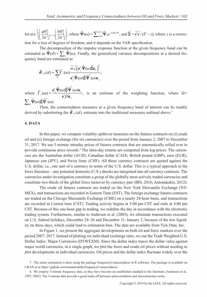
In Figure 1, we present the aggregate developments on both oil and forex markets over the period 2007–2017. Instead of plotting six individual exchange rates, we use the Trade Weighted U.S. Dollar Index: Major Currencies (DTWEXM). Since the dollar index traces the dollar value against major world currencies, in a single graph, we plot the forex and crude oil prices without needing to plot developments in individual currencies. Oil prices and the dollar index fluctuate widely over the

7. The entire estimation is done using the package frequencyConnectedness in R software. The package is available on CRAN or at https://github.com/tomaskrehlik/frequencyConnectedness.

8. We employ 5-minute frequency data, as they have become an established standard in the literature (Andersen et al., 1997, 2003). The 5-minute data provide a good trade-off between autocorrelation and microstructure noise.



period under investigation, which is in line with earlier assessments (Regnier, 2007; Baruník et al., 2015, 2017). The common pattern reveals that a rise (drop) in the oil price is associated with de-preciation (appreciation) of the U.S. dollar for most of the pictured period. This pattern is in accord with earlier findings for the pre-crisis period (Narayan et al., 2008; Akram, 2009). Further, Aloui et al. (2013) document that oil price increases are associated with dollar depreciation for most bilateral exchange rates, including the post-crisis period.

However, the above pattern does not hold universally. In 2010 and during late 2011–2014, rising oil prices correlate with appreciation of the dollar. Heterogeneity in the pattern might be grounded in the differences across countries with respect to oil dependence. Lizardo and Mollick (2010) show that rising oil prices lead to dollar depreciation with respect to currencies of countries that are net oil exporters (Canada, Mexico, and Russia) or countries that are neither net exporters nor significant importers of oil relative to their total trade (the U.K. and EU). On the other hand, an increase in oil prices leads to dollar appreciation with respect to the currencies of the net oil-im-porting countries such as Japan.9 Overall, Figure 1 provides persuasive evidence of strong linkages between the oil and forex markets.

5. RESULTS: TOTAL, ASYMMETRIC AND FREQUENCY CONNECTEDNESS

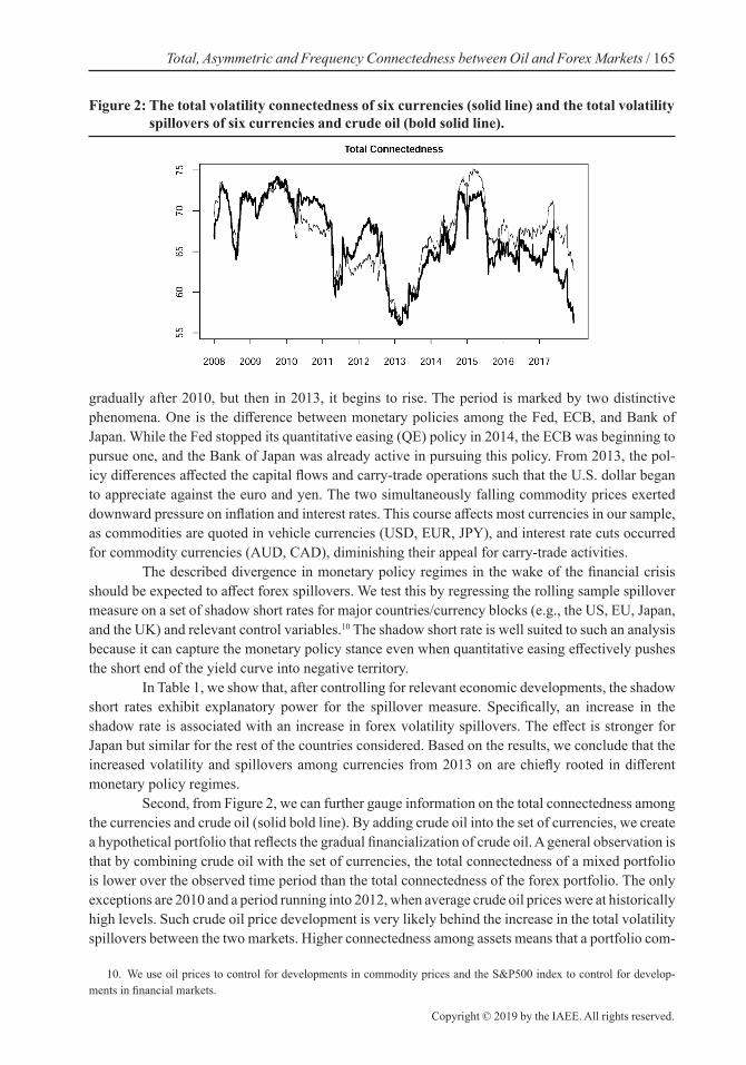
5.1 Total connectedness

In Figure 2, we present the total connectedness among the six currencies (solid line) along with the total connectedness among the currencies and oil (solid bold line). The total volatility spill-overs measure is calculated based on Diebold and Yilmaz (2012). First, we examine the connected-ness on the forex market (solid line): the connectedness is quite high during the GFC period until 2010 and then in 2012 and early 2014. The total connectedness values of 65% and above during the 2008–2010 period are comparable to those found in Diebold and Yilmaz (2015, Chapter 5). The plot exhibits a visible structural change in total connectedness among the six currencies under investigation: an initial high connectedness is interrupted by a short drop during 2009 and decreases

9. Heterogeneity in the pattern can also be associated with other factors, including US dependence on oil and net export position as well as the business cycle and source of a specific shock. These issues are beyond the scope of the paper and are left for further research.

Figure 1: Trade Weighted U.S. Dollar Index (solid line and left axis), crude oil (bold solid line and right axis



gradually after 2010, but then in 2013, it begins to rise. The period is marked by two distinctive phenomena. One is the difference between monetary policies among the Fed, ECB, and Bank of Japan. While the Fed stopped its quantitative easing (QE) policy in 2014, the ECB was beginning to pursue one, and the Bank of Japan was already active in pursuing this policy. From 2013, the pol-icy differences affected the capital flows and carry-trade operations such that the U.S. dollar began to appreciate against the euro and yen. The two simultaneously falling commodity prices exerted downward pressure on inflation and interest rates. This course affects most currencies in our sample, as commodities are quoted in vehicle currencies (USD, EUR, JPY), and interest rate cuts occurred for commodity currencies (AUD, CAD), diminishing their appeal for carry-trade activities.

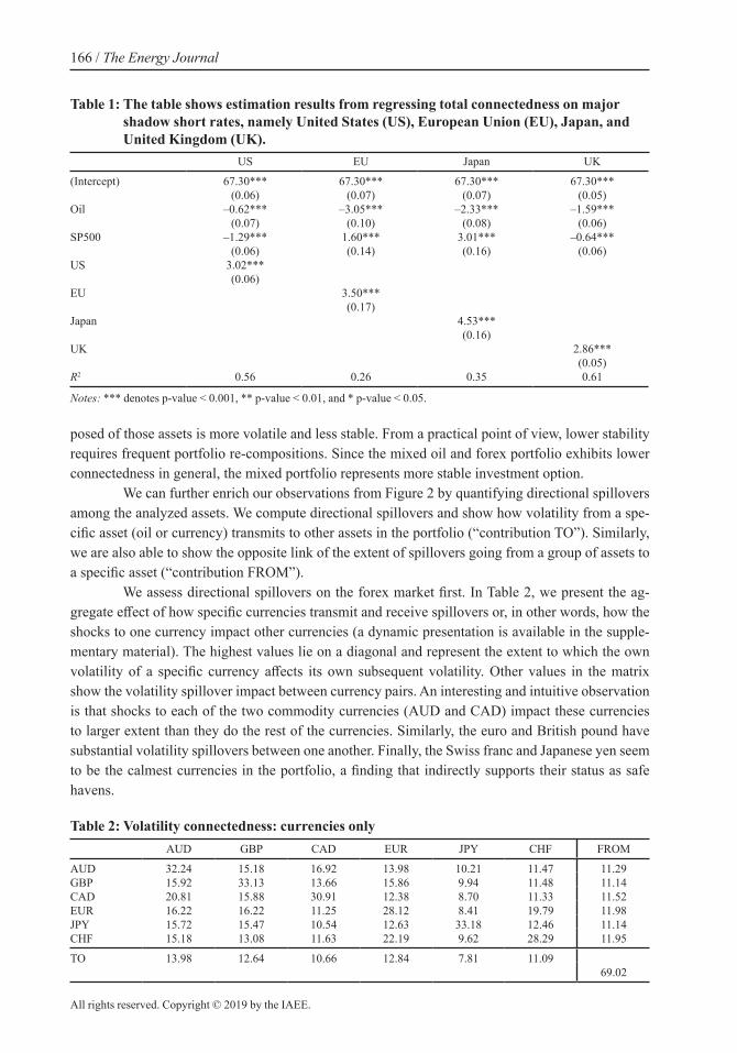
The described divergence in monetary policy regimes in the wake of the financial crisis should be expected to affect forex spillovers. We test this by regressing the rolling sample spillover measure on a set of shadow short rates for major countries/currency blocks (e.g., the US, EU, Japan, and the UK) and relevant control variables.10 The shadow short rate is well suited to such an analysis because it can capture the monetary policy stance even when quantitative easing effectively pushes the short end of the yield curve into negative territory.

In Table 1, we show that, after controlling for relevant economic developments, the shadow short rates exhibit explanatory power for the spillover measure. Specifically, an increase in the shadow rate is associated with an increase in forex volatility spillovers. The effect is stronger for Japan but similar for the rest of the countries considered. Based on the results, we conclude that the increased volatility and spillovers among currencies from 2013 on are chiefly rooted in different monetary policy regimes.

Second, from Figure 2, we can further gauge information on the total connectedness among the currencies and crude oil (solid bold line). By adding crude oil into the set of currencies, we create a hypothetical portfolio that reflects the gradual financialization of crude oil. A general observation is that by combining crude oil with the set of currencies, the total connectedness of a mixed portfolio is lower over the observed time period than the total connectedness of the forex portfolio. The only exceptions are 2010 and a period running into 2012, when average crude oil prices were at historically high levels. Such crude oil price development is very likely behind the increase in the total volatility spillovers between the two markets. Higher connectedness among assets means that a portfolio com-

10. We use oil prices to control for developments in commodity prices and the S&P500 index to control for develop-ments in financial markets.

Figure 2: The total volatility connectedness of six currencies (solid line) and the total volatility spillovers of six currencies and crude oil (bold solid line).



posed of those assets is more volatile and less stable. From a practical point of view, lower stability requires frequent portfolio re-compositions. Since the mixed oil and forex portfolio exhibits lower connectedness in general, the mixed portfolio represents more stable investment option.

We can further enrich our observations from Figure 2 by quantifying directional spillovers among the analyzed assets. We compute directional spillovers and show how volatility from a spe-cific asset (oil or currency) transmits to other assets in the portfolio (“contribution TO”). Similarly, we are also able to show the opposite link of the extent of spillovers going from a group of assets to a specific asset (“contribution FROM”).

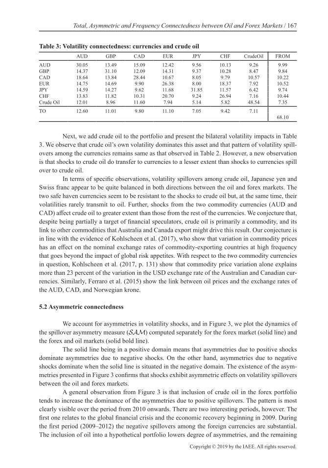
We assess directional spillovers on the forex market first. In Table 2, we present the ag-gregate effect of how specific currencies transmit and receive spillovers or, in other words, how the shocks to one currency impact other currencies (a dynamic presentation is available in the supple-mentary material). The highest values lie on a diagonal and represent the extent to which the own volatility of a specific currency affects its own subsequent volatility. Other values in the matrix show the volatility spillover impact between currency pairs. An interesting and intuitive observation is that shocks to each of the two commodity currencies (AUD and CAD) impact these currencies to larger extent than they do the rest of the currencies. Similarly, the euro and British pound have substantial volatility spillovers between one another. Finally, the Swiss franc and Japanese yen seem to be the calmest currencies in the portfolio, a finding that indirectly supports their status as safe havens.

Table 2: Volatility connectedness: currencies onlyAUD GBP CAD EUR JPY CHF FROM

AUD 32.24 15.18 16.92 13.98 10.21 11.47 11.29GBP 15.92 33.13 13.66 15.86 9.94 11.48 11.14CAD 20.81 15.88 30.91 12.38 8.70 11.33 11.52EUR 16.22 16.22 11.25 28.12 8.41 19.79 11.98JPY 15.72 15.47 10.54 12.63 33.18 12.46 11.14CHF 15.18 13.08 11.63 22.19 9.62 28.29 11.95

TO 13.98 12.64 10.66 12.84 7.81 11.0969.02

Table 1: The table shows estimation results from regressing total connectedness on major shadow short rates, namely United States (US), European Union (EU), Japan, and United Kingdom (UK).

US EU Japan UK

(Intercept) 67.30*** 67.30*** 67.30*** 67.30*** (0.06) (0.07) (0.07) (0.05)

Oil –0.62*** –3.05*** –2.33*** –1.59*** (0.07) (0.10) (0.08) (0.06)

SP500 –1.29*** 1.60*** 3.01*** –0.64*** (0.06) (0.14) (0.16) (0.06)

US 3.02*** (0.06)

EU 3.50*** (0.17)

Japan 4.53*** (0.16)

UK 2.86*** (0.05)

R2 0.56 0.26 0.35 0.61

Notes: *** denotes p-value < 0.001, ** p-value < 0.01, and * p-value < 0.05.



Table 3: Volatility connectedness: currencies and crude oilAUD GBP CAD EUR JPY CHF CrudeOil FROM

AUD 30.05 13.49 15.09 12.42 9.56 10.13 9.26 9.99GBP 14.37 31.10 12.09 14.31 9.37 10.28 8.47 9.84CAD 18.64 13.84 28.44 10.67 8.05 9.79 10.57 10.22EUR 14.75 14.69 9.90 26.38 8.00 18.37 7.92 10.52JPY 14.59 14.27 9.62 11.68 31.85 11.57 6.42 9.74CHF 13.83 11.82 10.31 20.70 9.24 26.94 7.16 10.44Crude Oil 12.01 8.96 11.60 7.94 5.14 5.82 48.54 7.35

TO 12.60 11.01 9.80 11.10 7.05 9.42 7.1168.10

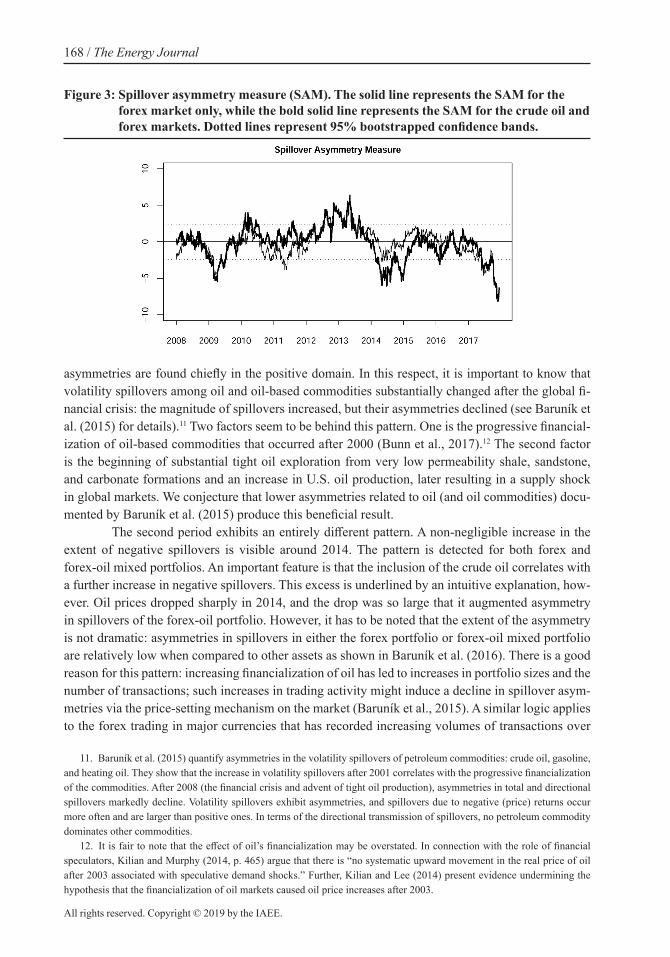
Next, we add crude oil to the portfolio and present the bilateral volatility impacts in Table 3. We observe that crude oil’s own volatility dominates this asset and that pattern of volatility spill-overs among the currencies remains same as that observed in Table 2. However, a new observation is that shocks to crude oil do transfer to currencies to a lesser extent than shocks to currencies spill over to crude oil.

In terms of specific observations, volatility spillovers among crude oil, Japanese yen and Swiss franc appear to be quite balanced in both directions between the oil and forex markets. The two safe haven currencies seem to be resistant to the shocks to crude oil but, at the same time, their volatilities rarely transmit to oil. Further, shocks from the two commodity currencies (AUD and CAD) affect crude oil to greater extent than those from the rest of the currencies. We conjecture that, despite being partially a target of financial speculators, crude oil is primarily a commodity, and its link to other commodities that Australia and Canada export might drive this result. Our conjecture is in line with the evidence of Kohlscheen et al. (2017), who show that variation in commodity prices has an effect on the nominal exchange rates of commodity-exporting countries at high frequency that goes beyond the impact of global risk appetites. With respect to the two commodity currencies in question, Kohlscheen et al. (2017, p. 131) show that commodity price variation alone explains more than 23 percent of the variation in the USD exchange rate of the Australian and Canadian cur-rencies. Similarly, Ferraro et al. (2015) show the link between oil prices and the exchange rates of the AUD, CAD, and Norwegian krone.

5.2 Asymmetric connectedness

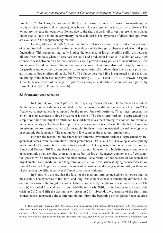
We account for asymmetries in volatility shocks, and in Figure 3, we plot the dynamics of the spillover asymmetry measure () computed separately for the forex market (solid line) and the forex and oil markets (solid bold line).

The solid line being in a positive domain means that asymmetries due to positive shocks dominate asymmetries due to negative shocks. On the other hand, asymmetries due to negative shocks dominate when the solid line is situated in the negative domain. The existence of the asym-metries presented in Figure 3 confirms that shocks exhibit asymmetric effects on volatility spillovers between the oil and forex markets.

A general observation from Figure 3 is that inclusion of crude oil in the forex portfolio tends to increase the dominance of the asymmetries due to positive spillovers. The pattern is most clearly visible over the period from 2010 onwards. There are two interesting periods, however. The first one relates to the global financial crisis and the economic recovery beginning in 2009. During the first period (2009–2012) the negative spillovers among the foreign currencies are substantial. The inclusion of oil into a hypothetical portfolio lowers degree of asymmetries, and the remaining



asymmetries are found chiefly in the positive domain. In this respect, it is important to know that volatility spillovers among oil and oil-based commodities substantially changed after the global fi-nancial crisis: the magnitude of spillovers increased, but their asymmetries declined (see Baruník et al. (2015) for details).11 Two factors seem to be behind this pattern. One is the progressive financial-ization of oil-based commodities that occurred after 2000 (Bunn et al., 2017).12 The second factor is the beginning of substantial tight oil exploration from very low permeability shale, sandstone, and carbonate formations and an increase in U.S. oil production, later resulting in a supply shock in global markets. We conjecture that lower asymmetries related to oil (and oil commodities) docu-mented by Baruník et al. (2015) produce this beneficial result.

The second period exhibits an entirely different pattern. A non-negligible increase in the extent of negative spillovers is visible around 2014. The pattern is detected for both forex and forex-oil mixed portfolios. An important feature is that the inclusion of the crude oil correlates with a further increase in negative spillovers. This excess is underlined by an intuitive explanation, how-ever. Oil prices dropped sharply in 2014, and the drop was so large that it augmented asymmetry in spillovers of the forex-oil portfolio. However, it has to be noted that the extent of the asymmetry is not dramatic: asymmetries in spillovers in either the forex portfolio or forex-oil mixed portfolio are relatively low when compared to other assets as shown in Baruník et al. (2016). There is a good reason for this pattern: increasing financialization of oil has led to increases in portfolio sizes and the number of transactions; such increases in trading activity might induce a decline in spillover asym-metries via the price-setting mechanism on the market (Baruník et al., 2015). A similar logic applies to the forex trading in major currencies that has recorded increasing volumes of transactions over

11. Baruník et al. (2015) quantify asymmetries in the volatility spillovers of petroleum commodities: crude oil, gasoline, and heating oil. They show that the increase in volatility spillovers after 2001 correlates with the progressive financialization of the commodities. After 2008 (the financial crisis and advent of tight oil production), asymmetries in total and directional spillovers markedly decline. Volatility spillovers exhibit asymmetries, and spillovers due to negative (price) returns occur more often and are larger than positive ones. In terms of the directional transmission of spillovers, no petroleum commodity dominates other commodities.

12. It is fair to note that the effect of oil’s financialization may be overstated. In connection with the role of financial speculators, Kilian and Murphy (2014, p. 465) argue that there is “no systematic upward movement in the real price of oil after 2003 associated with speculative demand shocks.” Further, Kilian and Lee (2014) present evidence undermining the hypothesis that the financialization of oil markets caused oil price increases after 2003.

Figure 3: Spillover asymmetry measure (SAM). The solid line represents the SAM for the forex market only, while the bold solid line represents the SAM for the crude oil and forex markets. Dotted lines represent 95% bootstrapped confidence bands.



time (BIS, 2016). Thus, the combined effect of the massive volume of transactions involving the two types of assets (oil and currencies) contributes to lower asymmetries in volatility spillovers. The temporary increase in negative spillovers due to the sharp drop in oil prices represents an isolated factor that is likely behind the asymmetry increase in 2014. The dynamics of directional spillovers are available in the supplementary material.

Finally, Aloui et al. (2013) argue that higher oil reserves and better production positions of a country help to reduce the extreme dependence of its foreign exchange market on oil price fluctuations. This statement indirectly implies the existence of lower volatility spillovers between oil and forex markets when oil reserves are solid and production is stable. In a similar way, high connectedness between oil and forex markets should prevail during periods of unavailability. Low inventories of crude oil force refineries to buy extra crude oil and may also lead to supply problems for gasoline and other petroleum products; low inventories of crude oil then likely cause price vol-atility and spillovers (Baruník et al., 2015). The above-described link is supported by the fact that the timing of the increased negative spillovers during 2010–2011 and 2013–2014 shown in Figure 3 match the occurrence of the negative spillovers among oil and oil-based commodities reported by Baruník et al. (2015, Figure 3, panel b).

5.3 Frequency connectedness

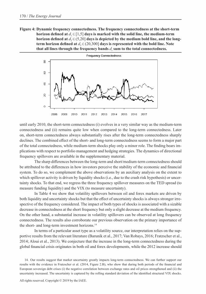
In Figure 4, we present plots of the frequency connectedness. The frequencies at which the frequency connectedness is computed can be understood as different investment horizons.13 The frequency connectedness is computed for the mixed forex-oil portfolio. Three lines represent the extent of connectedness at three investment horizons. The short-term horizon is represented by a simple solid line and might be attributed to short-term investment strategies adopted, for example, in technical analysis. The bold line represents the long-run connectedness. It reflects the long-term investment horizon associated with, for example, funds or investors oriented toward developments in economic fundamentals. The medium bold line captures the medium-term horizon.

Further, the reason that investors favor different investment horizons (represented by fre-quencies) comes from the formation of their preferences. Ortu et al. (2013) develop an asset pricing model in which consumption responds to shocks due to heterogeneous preference choices. Further, Bandi and Tamoni (2017) argue that investors may not focus on very high-frequency components of consumption representing short-term noise but on lower frequency components of consump-tion growth with heterogeneous periodicities instead. As a result, various sources of connectedness might create short-, medium-, and long-term systemic risk. Thus, when studying connectedness, we should focus on linkages with various degrees of persistence underlying systemic risk, as these are likely driving the differences over different investment horizons.

In Figure 4, we show that the level of the medium-term connectedness is lowest and the most stable. The dynamics of the short- and long-term connectedness is remarkably different. First, on three occasions, the long-term connectedness dramatically heightens. These increases correlate with (i) the global financial crisis from mid-2008 into early 2010, (ii) the European sovereign debt crisis in 2012, and (iii) the decline in oil prices in 2014. Second, the dynamics of the short-term connectedness represent quite a different picture. From the beginning of the global financial crisis

13. The short-term horizon of [1,5] days represents a business week, the medium-term horizon of (5,20] days represents a business month, and the long-term horizon of (20,300] days stands for a business year. These definitions represent differ-ent horizons from an investment perspective. Other horizons that represent reasonable alternative intervals deliver similar results. However, the plotted distinctions are less sharp than those provided by our choice of business week, month and year.



until early 2010, the short-term connectedness (i) evolves in a very similar way as the medium-term connectedness and (ii) remains quite low when compared to the long-term connectedness. Later on, short-term connectedness always substantially rises after the long-term connectedness sharply declines. The combined effect of the short- and long-term connectedness seems to form a major part of the total connectedness, while medium-term shocks play only a minor role. The finding bears im-plications with respect to portfolio management and hedging strategies. The dynamics of directional frequency spillovers are available in the supplementary material.

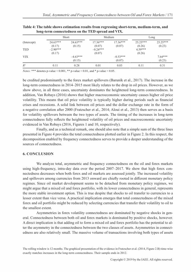
The sharp differences between the long-term and short/medium-term connectedness should be attributed to the differences in how investors perceive the stability of the economic and financial system. To do so, we complement the above observations by an auxiliary analysis on the extent to which spillover activity is driven by liquidity shocks (i.e., due to the crash risk hypothesis) or uncer-tainty shocks. To that end, we regress the three frequency spillover measures on the TED spread (to measure funding liquidity) and the VIX (to measure uncertainty).

In Table 4 we show that volatility spillovers between oil and forex markets are driven by both liquidity and uncertainty shocks but that the effect of uncertainty shocks is always stronger irre-spective of the frequency considered. The impact of both types of shocks is associated with a sizable decrease in connectedness at the short frequency but only a slight decrease at the medium frequency. On the other hand, a substantial increase in volatility spillovers can be observed at long frequency connectedness. The results also corroborate our previous observation on the primary importance of the short- and long-term investment horizons.14

In terms of a particular asset type as a volatility source, our interpretation relies on the sup-portive results from the relevant literature (Baruník et al., 2017; Van Robays, 2016; Fratzscher et al., 2014; Aloui et al., 2013). We conjecture that the increase in the long-term connectedness during the global financial crisis originates in both oil and forex developments, while the 2012 increase should

14. Our results suggest that market uncertainty greatly impacts long-term connectedness. We can further support our results with the evidence in Fratzscher et al. (2014, Figure 2.B), who show that during both periods of the financial and European sovereign debt crises (i) the negative correlation between exchange rates and oil prices strengthened and (ii) the uncertainty increased. The uncertainty is captured by the rolling standard deviation of the identified structural VIX shocks.

Figure 4: Dynamic frequency connectedness. The frequency connectedness at the short-term horizon defined at d1 [1,5] days is marked with the solid line, the medium-term horizon defined at d2 (5,20] days is depicted by the medium bold line, and the long-term horizon defined at d3 (20,300] days is represented with the bold line. Note that all lines through the frequency bands ds sum to the total connectedness.



be credited predominantly to the forex market spillovers (Baruník et al., 2017). The increase in the long-term connectedness in 2014–2015 most likely relates to the drop in oil prices. However, as we show above, in all three cases, uncertainty dominates the heightened long-term connectedness. In addition, Van Robays (2016) shows that higher macroeconomic uncertainty causes higher oil price volatility. This means that oil price volatility is typically higher during periods such as financial crises and recessions. A solid link between oil prices and the dollar exchange rate in the form of a negative correlation after 2000 (Fratzscher et al., 2014; Aloui et al., 2013) then serves as a basis for volatility spillovers between the two types of assets. The timing of the increases in long-term connectedness fully reflects the heightened volatility of oil prices and macroeconomic uncertainty evidenced in Van Robays (2016, Figures 1 and 10, respectively).

Finally, and as a technical remark, one should also note that a simple sum of the three lines presented in Figure 4 provides the total connectedness plotted earlier in Figure 2. In this respect, the decomposition enabled by frequency connectedness serves to provide a deeper understanding of the sources of connectedness.

6. CONCLUSION

We analyze total, asymmetric and frequency connectedness on the oil and forex markets using high-frequency, intra-day data over the period 2007–2017. We show that high forex con-nectedness decreases when both forex and oil markets are assessed jointly. The increased volatility and spillovers among currencies from 2013 onward are chiefly rooted in different monetary policy regimes. Since oil market development seems to be detached from monetary policy regimes, we might argue that a mixed oil and forex portfolio, with its lower connectedness in general, represents the more stable investment option. This is true despite that shocks to oil transfer to currencies to a lesser extent than vice versa. A practical implication emerges that total connectedness of the mixed forex and oil portfolio might be reduced by selecting currencies that transfer their volatility to oil to the smallest extent.

Asymmetries in forex volatility connectedness are dominated by negative shocks in gen-eral. Connectedness between both oil and forex markets is dominated by positive shocks, however. A direct implication is that adding oil to form a mixed oil and forex portfolio has the potential to al-ter the asymmetry in the connectedness between the two classes of assets. Asymmetries in connect-edness are also relatively small. The massive volume of transactions involving both types of assets

The rolling window is 12 months. The graphical presentation of the evidence in Fratzscher et al. (2014, Figure 2.B) time-wise exactly matches increases in the long-term connectedness. Their sample ends in 2012.

Table 4: The table shows estimation results from regressing short-term, medium-term, and long-term connectedness on the TED spread and VIX.

Short Medium Long

(Intercept) 24.63*** 24.63*** 17.36*** 17.36*** 25.25*** 25.25*** (0.17) (0.15) (0.07) (0.07) (0.26) (0.23)

TED –2.90*** –0.24*** 4.59*** (0.17) (0.07) (0.26)

VIX –4.63*** –0.53*** 7.64*** (0.15) (0.07) (0.23)

R2 0.11 0.28 0.01 0.03 0.11 0.31

Notes: *** denotes p-value < 0.001, ** p-value < 0.01, and * p-value < 0.05.



represents enormous information flows on both markets. We conjecture that ample information is likely behind the limited extent of asymmetries in volatility spillovers.

The dynamics of frequency connectedness differ dramatically across various investment horizons and should be credited to differences in investment preference formation. Frequency con-nectedness is to an extent driven by both liquidity and uncertainty shocks, and uncertainty shocks always exert a stronger impact irrespective of frequency. Both types of shocks suppress short-term connectedness but substantially raise long-term connectedness. This finding helps to explain fre-quency connectedness behavior, in that long-term connectedness reflects substantive features of economic development and investors’ concerns. Hence, frequency connectedness can also serve as a sensitive indicator of the horizon at which markets feel uncertainty the most.

ACKNOWLEDGMENTS

We are thankful for valuable comments we received from the editor Fredj Jawadi, Vá-clav Brož, Julien Chevallier, Lutz Kilian, four anonymous referees, and participants in the Fifth International Symposium in Computational Economics and Finance (ISCEF) in Paris, and other presentations. Part of the paper was written while Kočenda was a GEMCLINE visiting researcher at the Energy Center of the University of Auckland, whose hospitality is acknowledged. The usual disclaimer applies. Kočenda acknowledges support from the GAČR grant 19-15650S.

REFERENCES

Aboura, S. and J. Chevallier (2014). “Cross-market spillovers with ‘volatility surprise’.” Review of Financial Economics 23(4): 194–207. https://doi.org/10.1016/j.rfe.2014.08.002.

Akram, Q.F. (2009). “Commodity prices, interest rates and the dollar.” Energy economics 31(6): 838–851. https://doi.org/10.1016/j.eneco.2009.05.016.

Aloui, R., M. S. B. Assa, and D. K. Nguyen (2013). “Conditional dependence structure between oil prices and exchange rates: a copula-garch approach.” Journal of International Money and Finance 32: 719–738. https://doi.org/10.1016/j.ji-monfin.2012.06.006.

Andersen, T.G., T. Bollerslev, et al. (1997). “Intraday periodicity and volatility persistence in financial markets.” Journal of empirical finance 4(2–3): 115–158. https://doi.org/10.1016/S0927-5398(97)00004-2.

Andersen, T.G., T. Bollerslev, F.X. Diebold, and C. Vega (2003). “Micro effects of macro announcements: Real-time price discovery in foreign exchange.” American Economic Review 93(1): 38–62. https://doi.org/10.1257/000282803321455151.

Antonakakis, N. (2012). “Exchange return co-movements and volatility spillovers before and after the introduction of euro.” Journal of International Financial Markets, Institutions and Money 22(5): 1091–1109. https://doi.org/10.1016/j.int-fin.2012.05.009.

Antonakakis, N., J. Cunado, G. Filis, D. Gabauer, and F.P. De Gracia (2018). “Oil volatility, oil and gas firms and portfolio diversification.” Energy Economics 70: 499–515. https://doi.org/10.1016/j.eneco.2018.01.023.

Antonakakis, Nikolaos, J. Cunado, G. Filis, D. Gabauer, and F.P. De Gracia (2019). “Oil And Asset Classes Implied Vola-tilities: Dynamic Connectedness And Investment Strategies.” Available at SSRN: https://ssrn.com/abstract=3399996 or https://doi.org/10.2139/ssrn.3399996.

Arouri, M.E.H., J. Jouini, and D.K. Nguyen (2012). “On the impacts of oil price fluctuations on european equity mar-kets: Volatility spillover and hedging effectiveness.” Energy Economics 34(2): 611–617. https://doi.org/10.1016/j.eneco.2011.08.009.

Baker, H.K., G. Filbeck, and J.H. Harris (2018). Commodities: Markets, Performance, and Strategies. Oxford University Press. https://doi.org/10.1093/oso/9780190656010.003.0001.

Bandi, F.M., S. Chaudhuri, A.W. Lo, and A. Tamoni (2019). “Spectral Factor Models.” Johns Hopkins Carey Business School Research Paper No. 18-17. Available at SSRN: https://ssrn.com/abstract=3275567 or https://doi.org/10.2139/ssrn.3275567.

Barndorff-Nielsen, O., S. Kinnebrock, and N. Shephard (2010). Volatility and Time Series Econometrics: Essays in Honor of Robert F. Engle, Chapter Measuring Downside Risk-Realised Semivariance. Oxford University Press. https://doi.org/10.1093/acprof:oso/9780199549498.003.0007.



Baruník, J., E. Kočenda, and L. Vácha (2015). “Volatility spillovers across petroleum markets.” The Energy Journal 36(3): 309–329. https://doi.org/10.5547/01956574.36.3.jbar.

Baruník, J., E. Kočenda, and L. Vácha (2016). “Asymmetric connectedness on the US stock market: Bad and good volatility spillovers.” Journal of Financial Markets 27: 55–78. https://doi.org/10.1016/j.finmar.2015.09.003.

Baruník, J., E. Kočenda, and L. Vácha (2017). “Asymmetric volatility connectedness on the forex market.” Journal of Inter-national Money and Finance 77: 39–56. https://doi.org/10.1016/j.jimonfin.2017.06.003.

Baruník, J. and T. Křehlík (2018). “Measuring the frequency dynamics of financial connectedness and systemic risk.” Journal of Financial Econometrics 16(2): 271–296. https://doi.org/10.1093/jjfinec/nby001.

BIS (2016). Triennial central bank survey foreign exchange turnover in April 2016. available online (www.bis.org/publ/rpfx16.htm). Technical report, Bank for International Settlements (BIS).

Bubák, V., E. Kočenda, and F. Žikeš (2011). “Volatility transmission in emerging European foreign exchange markets.” Jour-nal of Banking & Finance 35(11): 2829–2841. https://doi.org/10.1016/j.jbankfin.2011.03.012.

Bunn, D.W., J. Chevallier, Y. Le Pen, and B. Sevi (2017). “Fundamental and financial influences on the co-movement of oil and gas prices.” The Energy Journal 38(2): 201–228. https://doi.org/10.5547/01956574.38.2.dbun.

Chang, C.-L., M. McAleer, and R. Tansuchat (2010). “Analyzing and forecasting volatility spillovers, asymmetries and hedg-ing in major oil markets.” Energy Economics 32(6): 1445–1455. https://doi.org/10.1016/j.eneco.2010.04.014.

Cogley, T. (2001). “A frequency decomposition of approximation errors in stochastic discount factor models.” International Economic Review 42(2): 473–503. https://doi.org/10.1111/1468-2354.00118.

Conlon, T., J. Cotter, and R. Gençay (2016). “Commodity futures hedging, risk aversion and the hedging horizon.” The Euro-pean Journal of Finance 22(15): 1534–1560. https://doi.org/10.1080/1351847X.2015.1031912.

Devereux, M.B., K. Shi, and J. Xu (2010). “Oil currency and the dollar standard: a simple analytical model of an international trade currency.” Journal of Money, Credit and Banking 42(4): 521–550. https://doi.org/10.1111/j.1538-4616.2010.00298.x.

Diebold, F. X. and K. Yilmaz (2009). Measuring financial asset return and volatility spillovers, with application to global equity markets. The Economic Journal 119(534): 158–171. https://doi.org/10.1111/j.1468-0297.2008.02208.x.

Diebold, F.X. and K. Yilmaz (2012). “Better to give than to receive: Predictive directional measurement of volatility spill-overs.” International Journal of Forecasting 28(1): 57–66. https://doi.org/10.1016/j.ijforecast.2011.02.006.

Diebold, F.X. and K. Yilmaz (2015). Financial and Macroeconomic Connectedness: A Network Approach to Measurement and Monitoring. Oxford University Press, USA. https://doi.org/10.1093/acprof:oso/9780199338290.001.0001.

Fattouh, B., L. Kilian, and L. Mahadeva (2013). “The role of speculation in oil markets: What have we learned so far?” The Energy Journal 34(3): 7–33. https://doi.org/10.5547/01956574.34.3.2.

Fattouh, B. and L. Mahadeva (2014). “Causes and implications of shifts in financial participation in commodity markets.” Journal of Futures Markets 34(8): 757–787. https://doi.org/10.1002/fut.21674.

Ferraro, D., K. Rogoff, and B. Rossi (2015). “Can oil prices forecast exchange rates? an empirical analysis of the relationship between commodity prices and exchange rates.” Journal of International Money and Finance 54: 116–141. https://doi.org/10.1016/j.jimonfin.2015.03.001.

Fratzscher, M., D. Schneider, and I. Van Robays (2014). Oil prices, exchange rates and asset prices. ECB Working Paper no. 1689. https://doi.org/10.2139/ssrn.2269027.

Gencay, R., N. Gradojevic, F. Selcuk, and B. Whitcher (2010). “Asymmetry of information flow between volatilities across time scales.” Quantitative Finance 10(8): 895–915. https://doi.org/10.1080/14697680903460143.

Greenwood-Nimmo, M., V.H. Nguyen, and B. Rafferty (2016). “Risk and return spillovers among the g10 currencies.” Jour-nal of Financial Markets 31: 43–62. https://doi.org/10.1016/j.finmar.2016.05.001.

Haigh, M.S. and M.T. Holt (2002). “Crack spread hedging: accounting for time-varying volatility spillovers in the energy futures markets.” Journal of Applied Econometrics 17(3): 269–289. https://doi.org/10.1002/jae.628.

Hammoudeh, S., H. Li, and B. Jeon (2003). “Causality and volatility spillovers among petroleum prices of WTI, gasoline and heating oil in different locations.” The North American Journal of Economics and Finance 14(1): 89–114. https://doi.org/10.1016/S1062-9408(02)00112-2.

Henriques, I. and P. Sadorsky (2011). “The effect of oil price volatility on strategic investment.” Energy Economics 33(1): 79–87. https://doi.org/10.1016/j.eneco.2010.09.001.

Kanas, A. (2001). “Volatility spillovers between stock returns and exchange rate changes: International evidence.” Journal of Business Finance & Accounting 27(3): 447–465. https://doi.org/10.1111/1468-5957.00320.

Kilian, L. (2009). “Not all oil price shocks are alike: Disentangling demand and supply shocks in the crude oil market.” Amer-ican Economic Review 99(3): 1053–69. https://doi.org/10.1257/aer.99.3.1053.

Kilian, L. and T.K. Lee (2014). “Quantifying the speculative component in the real price of oil: The role of global oil invento-ries.” Journal of International Money and Finance 42: 71–87. https://doi.org/10.1016/j.jimonfin.2013.08.005.



Kilian, L. and D.P. Murphy (2014). “The role of inventories and speculative trading in the global market for crude oil.” Jour-nal of Applied Econometrics 29(3): 454–478. https://doi.org/10.1002/jae.2322.

Kitamura, Y. (2010). “Testing for intraday interdependence and volatility spillover among the Euro, the pound and the Swiss franc markets.” Research in International Business and Finance 24(2): 158–171. https://doi.org/10.1016/j.ribaf.2009.11.002.

Kohlscheen, E., F. Avalos, and A. Schrimpf (2017). “When the walk is not random: Commodity prices and exchange rates.” International Journal of Central Banking 13(2): 121–158. https://doi.org/10.2139/ssrn.2740946.

Koop, G., M.H. Pesaran, and S.M. Potter (1996). “Impulse response analysis in nonlinear multivariate models.” Journal of Econometrics 74(1): 119–147. https://doi.org/10.1016/0304-4076(95)01753-4.

Lin, S.X. and M.N. Tamvakis (2001). “Spillover effects in energy futures markets.” Energy Economics 23(1): 43–56. https://doi.org/10.1016/S0140-9883(00)00051-7.

Lizardo, R.A. and A.V. Mollick (2010). “Oil price fluctuations and us dollar exchange rates.” Energy Economics 32(2): 399–408. https://doi.org/10.1016/j.eneco.2009.10.005.

Manera, M. (2013). “Introduction to a special issue on ‘financial speculation in the oil markets and the determinants of the price of oil’.” The Energy Journal 34(3): 1–5. https://doi.org/10.5547/01956574.34.3.1.

McMillan, D.G. and A.E. Speight (2010). “Return and volatility spillovers in three euro exchange rates.” Journal of Econom-ics and Business 62(2): 79–93. https://doi.org/10.1016/j.jeconbus.2009.08.003.

Narayan, P.K. and S. Narayan (2007). “Modelling oil price volatility.” Energy Policy 35(12): 6549–6553. https://doi.org/10.1016/j.enpol.2007.07.020.

Narayan, P.K., S. Narayan, and A. Prasad (2008). “Understanding the oil price-exchange rate nexus for the Fiji Islands.” En-ergy Economics 30(5): 2686–2696. https://doi.org/10.1016/j.eneco.2008.03.003.

Ortu, F., A. Tamoni, and C. Tebaldi (2013). “Long-run risk and the persistence of consumption shocks.” Review of Financial Studies 26(11): 2876–2915. https://doi.org/10.1093/rfs/hht038.

Patton, A.J. and K. Sheppard (2015). “Good volatility, bad volatility: Signed jumps and the persistence of volatility.” The Review of Economics and Statistics 97(3): 683–697. https://doi.org/10.1162/REST_a_00503.

Pesaran, H.H. and Y. Shin (1998). “Generalized impulse response analysis in linear multivariate models.” Economics letters 58(1): 17–29. https://doi.org/10.1016/S0165-1765(97)00214-0.

Pindyck, R.S. (2004). “Volatility in natural gas and oil markets.” The Journal of Energy and Development 30(1): 1–19.Regnier, E. (2007). “Oil and energy price volatility.” Energy Economics 29(3): 405–427. https://doi.org/10.1016/j.

eneco.2005.11.003.Restrepo, N., J. M. Uribe, and D. Manotas (2018). “Financial risk network architecture of energy firms.” Applied Energy 215:

630–642. https://doi.org/10.1016/j.apenergy.2018.02.060.Van Robays, I. (2016). “Macroeconomic uncertainty and oil price volatility.” Oxford Bulletin of Economics and Statistics

S(5): 671–693. https://doi.org/10.1111/obes.12124.

Documents

Total, Asymmetric and Frequency Connectedness between Oil