Embed Size (px)
Citation preview
Journal of Productivity Analysis, 14, 31–51 (2000)c© 2000 Kluwer Academic Publishers, Boston. Manufactured in The Netherlands.
Total Factor Productivity Growth and TechnicalChange in a Profit Function Framework
GIANNIS KARAGIANNISNational Agriculturan and Research Foundation, Department of Economics, University of Crete, Greece
GEORGE J. MERGOS [email protected] of Economics, University of Athens, Greece
Abstract
This paper develops a framework for measuring and decomposing TFP changes, withinthe parametric approach, by using directly the estimated parameters of a profit function.Two alternative relationships are derived for measuring and decomposing TFP changes viaa profit function based on two alternative definitions of the rate of technical change, i.e.,input- and output-based. Initially a long-run equilibrium framework is assumed and then theanalysis is extended to the case of temporary equilibrium. The latter framework is appliedto US agriculture by estimating a translog profit function and analyzing TFP changes duringthe period 1948–1994.
Keywords: TFP measurement and decomposition, profit function, technical change
1. Introduction
Accurate measures of Total Factor Productivity (TFP) and reliable decomposition of itssources can be obtained within the parametric approach only if the appropriate structural andbehavioral assumptions are correctly specified (Callan, 1991). Structural assumptions referto returns to scale, technical change, productive efficiency, and capacity utilization, whereasbehavioral assumptions refer to the objective function of the firm(s), market structure, andthe importance of various regulations. Most efforts to improve the theoretical frameworkof TFP measurement and attribution, using the parametric approach, have been based onduality and particularly, on cost function.1 Denny et al. (1981) considered the role oftechnical change and returns to scale in TFP changes for competitive, monopolistic andregulated firms. Morrison (1986), Berndt and Fuss (1986), and Nadiri and Prucha (1990)incorporated in addition the impact of capacity utilization in the case of competitive firms andMorrison (1992) extended it to monopolistic firms. Bauer (1990) considered the impactof productive efficiency on TFP changes for competitive and monopolistic firms, whileGranderson (1997) extended it to case of regulated firms.
Instead of a cost function, a profit function may also be used for parametrically measuringand decomposing TFP changes, on the basis of a different behavioral assumption. If firmsare profit maximizing, then it may be more appropriate to use the dual profit function rather
32 KARAGIANNIS AND MERGOS
than the cost function to represent the firm’s or industry’s production decisions (Ray andSegerson, 1991). This is more likely in the case of highly competitive industries, suchas services and small manufacturing, in which firms are price takers in input and outputmarkets and there are no production regulations.2 Use of the profit function allows bothoutput and input levels to be determined endogenously and to adjust accordingly to changesin prices and technology. This feature overcomes a serious limitation of the cost functionwhich assumes that output levels are not affected by factor price changes and thus, theindirect effect of these changes (via output levels) on factor demand is ignored (Lopez,1982).3 All the above are obtained at the cost of a stronger behavioral assumption, howeverprofit maximization always implies cost minimization while the opposite is not necessarilytrue.
There have been several previous attempts in developing a framework for measuringand decomposing TFP growth by using a profit function, but with limited success. Levy(1981), Ray and Segerson (1991) and Fox (1996) focused only on the measurement of therate of technical change via a profit function (i.e., the rate of profit augmentation). Otherstudies relied on information obtained from an estimated profit function but then used eitherindex numbers (i.e., Jayneet al., 1994; Coelli, 1996), or a primal approach (i.e., Luh andStefanou, 1991, 1993; Lynde and Richmond, 1993; Fousekis and Papakonstantinou, 1997)for measuring and decomposing TFP changes. Specifically, in their approach the estimatedprofit function is used only to compute shadow values of quasi-fixed inputs, which are thenutilized in Divisia index and in a production function based decomposition of TFP growth,respectively. Bernstein (1994) did the first attempt to develop a framework for measuringand decomposing TFP growth within a profit function using dual concepts, but presentedonly one side of the problem. In particular, he relied only on the input-based measure of therate of technical change, while as explained in the next section an output-based measure oftechnical change may also be defined within a profit function framework.
The main objective of this paper is to develop a framework for measuring and decompos-ing TFP changes, within the parametric approach, by using directly the estimated parametersof a profit function. Due to the endogeneity of both inputs and outputs in a profit functionframework, two measures of the rate of technical change (i.e., input- and output-based) canbe defined and consequently, two alternative relationships are developed for decomposingTFP changes. For the latter, we provide a slightly different, but easier to interpret, rela-tionship than that developed by Bernstein (1994). It is also shown that the two alternativedecomposition relationships provide similar information about the sources of TFP changes,but different quantitative results in the presence of non-constant returns to scale.
The rest of this paper proceeds as follows. Dual measures of the degree of returns toscale and of the rate of technical change within a profit function framework are developedin the next section. In the third section, we briefly examine (for purposes of completenessonly) the case of TFP decomposition within a long-run profit function framework and nextwe provide a rigorous treatment of the case of temporary equilibrium by using a restrictedprofit function, which is more relevant to empirical applications. An empirical applicationof this framework is presented in the fourth section by estimating a translog profit functionfor US agriculture using data of the period 1948–1994. Concluding remarks follow in thelast section.
PROFIT FUNCTION FRAMEWORK 33
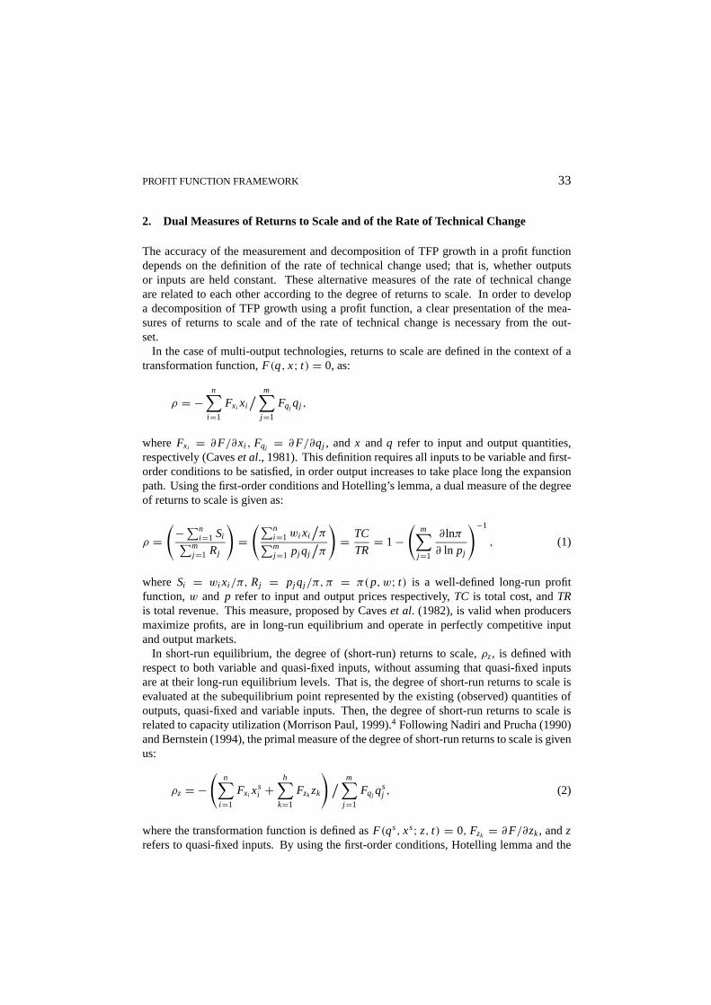
2. Dual Measures of Returns to Scale and of the Rate of Technical Change
The accuracy of the measurement and decomposition of TFP growth in a profit functiondepends on the definition of the rate of technical change used; that is, whether outputsor inputs are held constant. These alternative measures of the rate of technical changeare related to each other according to the degree of returns to scale. In order to developa decomposition of TFP growth using a profit function, a clear presentation of the mea-sures of returns to scale and of the rate of technical change is necessary from the out-set.
In the case of multi-output technologies, returns to scale are defined in the context of atransformation function,F(q, x; t) = 0, as:
ρ = −n∑
i=1
Fxi xi/ m∑
j=1
Fqj qj ,
whereFxi = ∂F/∂xi , Fqj = ∂F/∂qj , andx andq refer to input and output quantities,respectively (Caveset al., 1981). This definition requires all inputs to be variable and first-order conditions to be satisfied, in order output increases to take place long the expansionpath. Using the first-order conditions and Hotelling’s lemma, a dual measure of the degreeof returns to scale is given as:
ρ =(−∑n
i=1 Si∑mj=1 Rj
)=(∑n
i=1wi xi/π∑m
j=1 pj qj/π
)= TC
TR= 1−
(m∑
j=1
∂ lnπ
∂ ln pj
)−1
, (1)
where Si = wi xi /π, Rj = pj qj /π, π = π(p, w; t) is a well-defined long-run profitfunction,w and p refer to input and output prices respectively,TC is total cost, andTRis total revenue. This measure, proposed by Caveset al. (1982), is valid when producersmaximize profits, are in long-run equilibrium and operate in perfectly competitive inputand output markets.
In short-run equilibrium, the degree of (short-run) returns to scale,ρz, is defined withrespect to both variable and quasi-fixed inputs, without assuming that quasi-fixed inputsare at their long-run equilibrium levels. That is, the degree of short-run returns to scale isevaluated at the subequilibrium point represented by the existing (observed) quantities ofoutputs, quasi-fixed and variable inputs. Then, the degree of short-run returns to scale isrelated to capacity utilization (Morrison Paul, 1999).4 Following Nadiri and Prucha (1990)and Bernstein (1994), the primal measure of the degree of short-run returns to scale is givenus:
ρz = −(
n∑i=1
Fxi xsi +
h∑k=1
Fzk zk
)/ m∑j=1
Fqj qsj , (2)
where the transformation function is defined asF(qs, xs; z, t) = 0, Fzk = ∂F/∂zk, andzrefers to quasi-fixed inputs. By using the first-order conditions, Hotelling lemma and the
34 KARAGIANNIS AND MERGOS
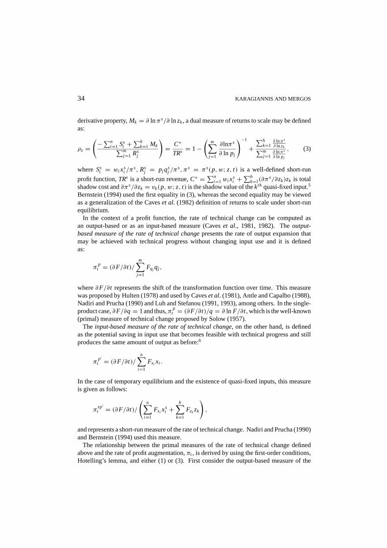
derivative property,Mk = ∂ lnπs/∂ ln zk, a dual measure of returns to scale may be definedas:
ρz =(−∑n
i=1 Ssi +
∑hk=1 Mk∑m
j=1 Rsj
)= C∗
TRs = 1−(
m∑j=1
∂ lnπs
∂ ln pj
)−1
+∑h
k=1∂ lnπs
∂ ln zk∑mj=1
∂ lnπs
∂ ln pj
, (3)
where Ssi = wi xs
i /πs, Rs
j = pj qsj /π
s, πs = πs(p, w; z, t) is a well-defined short-run
profit function,TRs is a short-run revenue,C∗ = ∑ni=1wi xs
i +∑h
k=1(∂πs/∂zk)zk is total
shadow cost and∂πs/∂zk = vk(p, w; z, t) is the shadow value of thekth quasi-fixed input.5
Bernstein (1994) used the first equality in (3), whereas the second equality may be viewedas a generalization of the Caveset al. (1982) definition of returns to scale under short-runequilibrium.
In the context of a profit function, the rate of technical change can be computed asan output-based or as an input-based measure (Caveset al., 1981, 1982). Theoutput-based measure of the rate of technical changepresents the rate of output expansion thatmay be achieved with technical progress without changing input use and it is definedas:
πpt = (∂F/∂t)/
m∑j=1
Fqj qj ,
where∂F/∂t represents the shift of the transformation function over time. This measurewas proposed by Hulten (1978) and used by Caveset al. (1981), Antle and Capalbo (1988),Nadiri and Prucha (1990) and Luh and Stefanou (1991, 1993), among others. In the single-product case,∂F/∂q = 1 and thus,π p
t = (∂F/∂t)/q = ∂ ln F/∂t , which is the well-known(primal) measure of technical change proposed by Solow (1957).
The input-based measure of the rate of technical change, on the other hand, is definedas the potential saving in input use that becomes feasible with technical progress and stillproduces the same amount of output as before:6
πp′t = (∂F/∂t)/
n∑i=1
Fxi xi .
In the case of temporary equilibrium and the existence of quasi-fixed inputs, this measureis given as follows:
πsp′t = (∂F/∂t)/
(n∑
i=1
Fxi xsi +
h∑k=1
Fzk zk
),
and represents a short-run measure of the rate of technical change. Nadiri and Prucha (1990)and Bernstein (1994) used this measure.
The relationship between the primal measures of the rate of technical change definedabove and the rate of profit augmentation,πt , is derived by using the first-order conditions,Hotelling’s lemma, and either (1) or (3). First consider the output-based measure of the
PROFIT FUNCTION FRAMEWORK 35
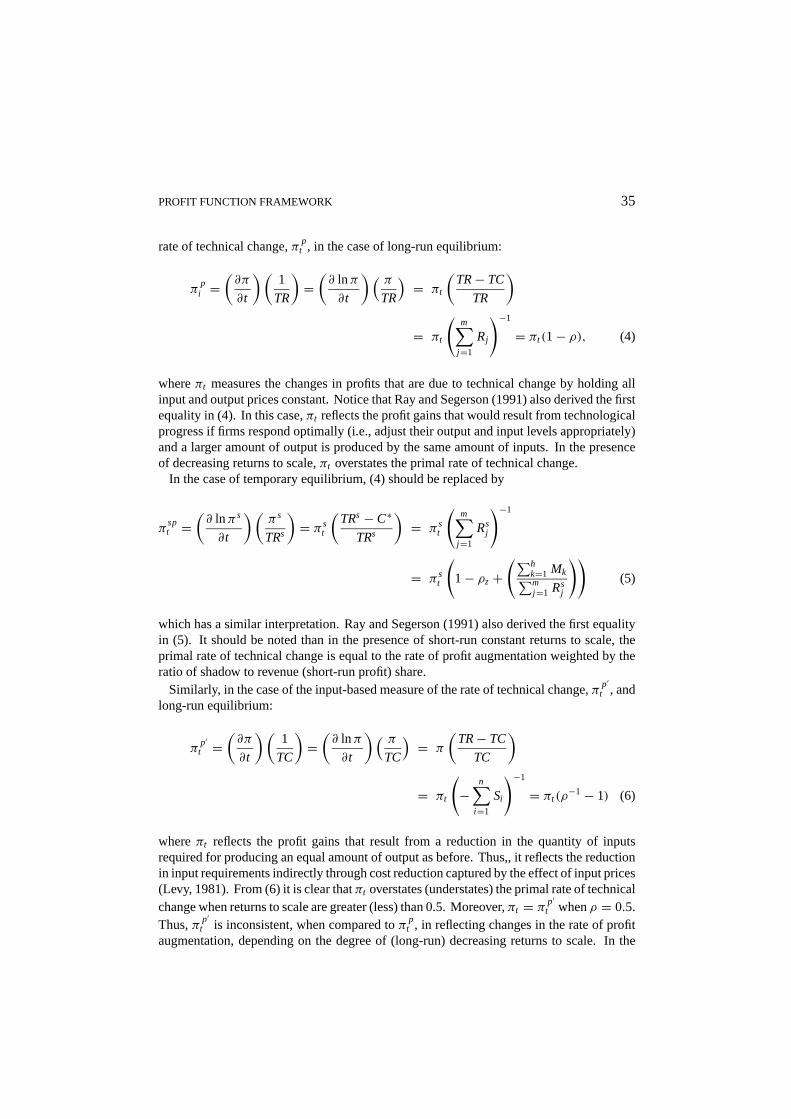
rate of technical change,π pt , in the case of long-run equilibrium:
πpi =
(∂π
∂t
)(1
TR
)=(∂ lnπ
∂t
)( πTR
)= πt
(TR− TC
TR
)
= πt
(m∑
j=1
Rj
)−1
= πt (1− ρ), (4)
whereπt measures the changes in profits that are due to technical change by holding allinput and output prices constant. Notice that Ray and Segerson (1991) also derived the firstequality in (4). In this case,πt reflects the profit gains that would result from technologicalprogress if firms respond optimally (i.e., adjust their output and input levels appropriately)and a larger amount of output is produced by the same amount of inputs. In the presenceof decreasing returns to scale,πt overstates the primal rate of technical change.
In the case of temporary equilibrium, (4) should be replaced by
πspt =
(∂ lnπs
∂t
)(πs
TRs
)= πs
t
(TRs − C∗
TRs
)= πs
t
(m∑
j=1
Rsj
)−1
= πst
(1− ρz+
(∑hk=1 Mk∑mj=1 Rs
j
))(5)
which has a similar interpretation. Ray and Segerson (1991) also derived the first equalityin (5). It should be noted than in the presence of short-run constant returns to scale, theprimal rate of technical change is equal to the rate of profit augmentation weighted by theratio of shadow to revenue (short-run profit) share.
Similarly, in the case of the input-based measure of the rate of technical change,πp′t , and
long-run equilibrium:
πp′t =
(∂π
∂t
)(1
TC
)=(∂ lnπ
∂t
)( πTC
)= π
(TR− TC
TC
)
= πt
(−
n∑i=1
Si
)−1
= πt (ρ−1− 1) (6)
whereπt reflects the profit gains that result from a reduction in the quantity of inputsrequired for producing an equal amount of output as before. Thus,, it reflects the reductionin input requirements indirectly through cost reduction captured by the effect of input prices(Levy, 1981). From (6) it is clear thatπt overstates (understates) the primal rate of technicalchange when returns to scale are greater (less) than 0.5. Moreover,πt = π p′
t whenρ = 0.5.Thus,π p′
t is inconsistent, when compared toπ pt , in reflecting changes in the rate of profit
augmentation, depending on the degree of (long-run) decreasing returns to scale. In the
36 KARAGIANNIS AND MERGOS
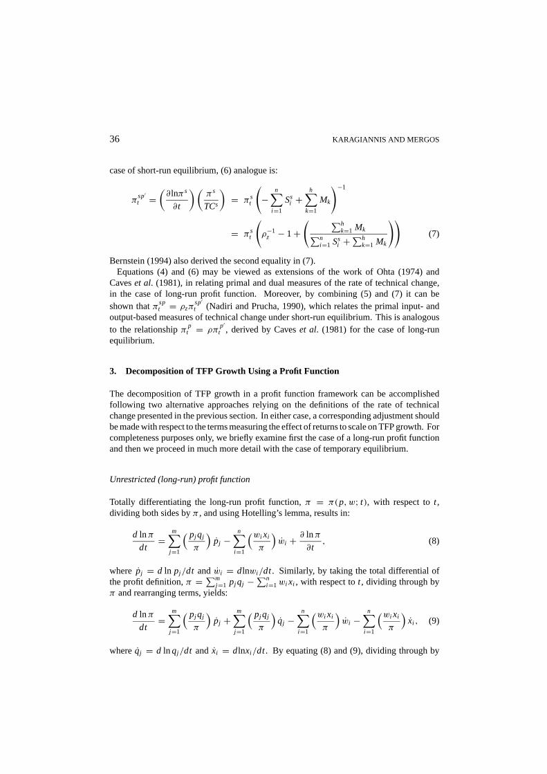
case of short-run equilibrium, (6) analogue is:
πsp′t =
(∂ lnπs
∂t
)(πs
TCs
)= πs
t
(−
n∑i=1
Ssi +
h∑k=1
Mk
)−1
= πst
(ρ−1
z − 1+( ∑h
k=1 Mk∑ni=1 Ss
i +∑h
k=1 Mk
))(7)
Bernstein (1994) also derived the second equality in (7).Equations (4) and (6) may be viewed as extensions of the work of Ohta (1974) and
Caveset al. (1981), in relating primal and dual measures of the rate of technical change,in the case of long-run profit function. Moreover, by combining (5) and (7) it can beshown thatπsp
t = ρzπsp′t (Nadiri and Prucha, 1990), which relates the primal input- and
output-based measures of technical change under short-run equilibrium. This is analogousto the relationshipπ p
t = ρπp′t , derived by Caveset al. (1981) for the case of long-run
equilibrium.
3. Decomposition of TFP Growth Using a Profit Function
The decomposition of TFP growth in a profit function framework can be accomplishedfollowing two alternative approaches relying on the definitions of the rate of technicalchange presented in the previous section. In either case, a corresponding adjustment shouldbe made with respect to the terms measuring the effect of returns to scale on TFP growth. Forcompleteness purposes only, we briefly examine first the case of a long-run profit functionand then we proceed in much more detail with the case of temporary equilibrium.
Unrestricted (long-run) profit function
Totally differentiating the long-run profit function,π = π(p, w; t), with respect tot ,dividing both sides byπ , and using Hotelling’s lemma, results in:
d lnπ
dt=
m∑j=1
( pj qj
π
)pj −
n∑i=1
(wi xi
π
)wi + ∂ lnπ
∂t, (8)
where pj = d ln pj /dt andwi = dlnwi /dt. Similarly, by taking the total differential ofthe profit definition,π = ∑m
j=1 pj qj −∑n
i=1wi xi , with respect tot , dividing through byπ and rearranging terms, yields:
d lnπ
dt=
m∑j=1
( pj qj
π
)pj +
m∑j=1
( pj qj
π
)qj −
n∑i=1
(wi xi
π
)wi −
n∑i=1
(wi xi
π
)xi , (9)
whereqj = d ln qj /dt and xi = dlnxi /dt. By equating (8) and (9), dividing through by
PROFIT FUNCTION FRAMEWORK 37
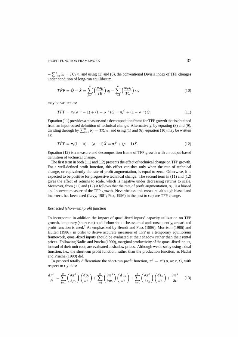
−∑ni=1 Si = TC/π , and using (1) and (6), the conventional Divisia index of TFP changes
under condition of long-run equilibrium,
TFP= Q− X =m∑
j=1
( pj qj
TR
)qj −
n∑i=1
(wi xi
TC
)xi , (10)
may be written as:
TFP= πt (ρ−1− 1)+ (1− ρ−1)Q = π p′
t + (1− ρ−1)Q. (11)
Equation (11) provides a measure and a decomposition frame for TFP growth that is obtainedfrom an input-based definition of technical change. Alternatively, by equating (8) and (9),dividing through by
∑mj=1 Rj = TR/π , and using (1) and (6), equation (10) may be written
as:
TFP= πt (1− ρ)+ (ρ − 1)X = π pt + (ρ − 1)X. (12)
Equation (12) is a measure and decomposition frame of TFP growth with an output-baseddefinition of technical change.
The first term in both (11) and (12) presents the effect of technical change on TFP growth.For a well-defined profit function, this effect vanishes only when the rate of technicalchange, or equivalently the rate of profit augmentation, is equal to zero. Otherwise, it isexpected to be positive for progressive technical change. The second term in (11) and (12)gives the effect of returns to scale, which is negative under decreasing returns to scale.Moreover, from (11) and (12) it follows that the rate of profit augmentation,πt , is a biasedand incorrect measure of the TFP growth. Nevertheless, this measure, although biased andincorrect, has been used (Levy, 1981; Fox, 1996) in the past to capture TFP change.
Restricted (short-run) profit function
To incorporate in addition the impact of quasi-fixed inputs’ capacity utilization on TFPgrowth, temporary (short-run) equilibrium should be assumed and consequently, a restrictedprofit function is used.7 As emphasized by Berndt and Fuss (1986), Morrison (1986) andHulten (1986), in order to derive accurate measures of TFP in a temporary equilibriumframework, quasi-fixed inputs should be evaluated at their shadow rather than their rentalprices. Following Nadiri and Prucha (1990), marginal productivity of the quasi-fixed inputs,instead of their unit cost, are evaluated at shadow prices. Although we do so by using a dualfunction, i.e., the short-run profit function, rather than the production function, as Nadiriand Prucha (1990) did.
To proceed totally differentiate the short-run profit function,πs = πs(p, w; z, t), withrespect tot yields:
dπs
dt=
m∑j=1
(∂πs
∂pj
)(dpj
dt
)+
n∑i=1
(∂πs
∂wi
)(dwi
dt
)+
h∑k=1
(∂πs
∂zk
)(dzk
dt
)+ ∂π
s
∂t. (13)
38 KARAGIANNIS AND MERGOS
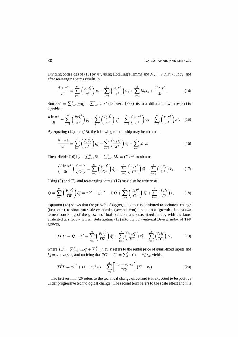
Dividing both sides of (13) byπs, using Hotelling’s lemma andMk = ∂ lnπs/∂ ln zk, andafter rearranging terms results in:
d lnπs
dt=
m∑j=1
(pj qs
j
πs
)pj −
n∑i=1
(wi xs
i
πs
)wi +
h∑k=1
Mkzk + ∂ lnπs
∂t. (14)
Sinceπs =∑mj=1 pj qs
j −∑n
i=1wi xsi (Diewert, 1973), its total differential with respect to
t yields:
d lnπs
dt=
m∑j=1
(pj qs
j
πs
)pj +
m∑j=1
(pj qs
j
πs
)qs
j −n∑
i=1
(wi xs
i
πs
)wi −
n∑i=1
(wi xs
i
πs
)xs
i . (15)
By equating (14) and (15), the following relationship may be obtained:
∂ lnπs
∂t=
m∑j=1
(pj qs
j
πs
)qs
j −n∑
i=1
(wi xs
i
πs
)xs
i −h∑
k=1
Mkzk. (16)
Then, divide (16) by−∑ni=1 Ss
i +∑h
k=1 Mk = C∗/πs to obtain:(∂ lnπs
∂t
)(πs
C∗
)=
m∑j=1
(pj qs
j
C∗
)qs
j −n∑
i=1
(wi xs
i
C∗
)xs
i −h∑
k=1
(vkzk
C∗)
zk. (17)
Using (3) and (7), and rearranging terms, (17) may also be written as:
Q =m∑
j=1
(pj qs
j
TRs
)qs
j = πsp′t + (ρ−1
z − 1)Q+n∑
i=1
(wi xs
i
C∗
)xs
i +h∑
k=1
(vkzk
C∗)
zk (18)
Equation (18) shows that the growth of aggregate output is attributed to technical change(first term), to short-run scale economies (second term), and to input growth (the last twoterms) consisting of the growth of both variable and quasi-fixed inputs, with the latterevaluated at shadow prices. Substituting (18) into the conventional Divisia index of TFPgrowth,
TFP′ = Q− X′ =m∑
j=1
(pj qs
j
TRs
)qs
j −n∑
i=1
(wi xs
i
TC′
)xs
i −h∑
k=1
(rkzk
TC′)
zk, (19)
whereTC′ =∑ni=1wi xs
i +∑h
k−1 rkzk, r refers to the rental price of quasi-fixed inputs andzk = d ln zk/dt, and noticing thatTC′ − C∗ =∑h
k=1(rk − vk)zk, yields:
TFP= πsp′t + (1− ρ−1
z )Q+h∑
i=1
[(rk − vk)zk
TCs
] (X′ − zk
)(20)
The first term in (20 refers to the technical change effect and it is expected to be positiveunder progressive technological change. The second term refers to the scale effect and it is
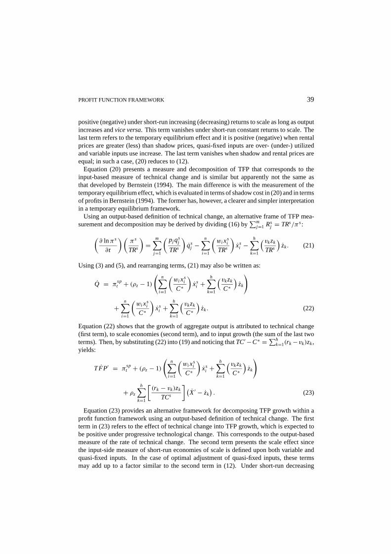
PROFIT FUNCTION FRAMEWORK 39
positive (negative) under short-run increasing (decreasing) returns to scale as long as outputincreases andvice versa. This term vanishes under short-run constant returns to scale. Thelast term refers to the temporary equilibrium effect and it is positive (negative) when rentalprices are greater (less) than shadow prices, quasi-fixed inputs are over- (under-) utilizedand variable inputs use increase. The last term vanishes when shadow and rental prices areequal; in such a case, (20) reduces to (12).
Equation (20) presents a measure and decomposition of TFP that corresponds to theinput-based measure of technical change and is similar but apparently not the same asthat developed by Bernstein (1994). The main difference is with the measurement of thetemporary equilibrium effect, which is evaluated in terms of shadow cost in (20) and in termsof profits in Bernstein (1994). The former has, however, a clearer and simpler interpretationin a temporary equilibrium framework.
Using an output-based definition of technical change, an alternative frame of TFP mea-surement and decomposition may be derived by dividing (16) by
∑mj=1 Rs
j = TRs/πs:(∂ lnπs
∂t
)(πs
TRs
)=
m∑j=1
(pj qs
j
TRs
)qs
j −n∑
i=1
(wi xs
i
TRs
)xs
i −h∑
k=1
(vkzk
TRs
)zk. (21)
Using (3) and (5), and rearranging terms, (21) may also be written as:
Q = πspt + (ρz− 1)
(n∑
i=1
(wi xs
i
C∗
)xs
i +h∑
k=1
(vkzk
C∗)
zk
)
+n∑
i=1
(wi xs
i
C∗
)xs
i +h∑
k=1
(vkzk
C∗)
zk. (22)
Equation (22) shows that the growth of aggregate output is attributed to technical change(first term), to scale economies (second term), and to input growth (the sum of the last twoterms). Then, by substituting (22) into (19) and noticing thatTC′ −C∗ =∑h
k=1(rk−vk)zk,yields:
TFP′ = πspt + (ρz− 1)
(n∑
i=1
(wi xs
i
C∗
)xs
i +h∑
k=1
(vkzk
C∗)
zk
)
+ ρz
h∑k=1
[(rk − vk)zk
TCs
] (X′ − zk
). (23)
Equation (23) provides an alternative framework for decomposing TFP growth within aprofit function framework using an output-based definition of technical change. The firstterm in (23) refers to the effect of technical change into TFP growth, which is expected tobe positive under progressive technological change. This corresponds to the output-basedmeasure of the rate of technical change. The second term presents the scale effect sincethe input-side measure of short-run economies of scale is defined upon both variable andquasi-fixed inputs. In the case of optimal adjustment of quasi-fixed inputs, these termsmay add up to a factor similar to the second term in (12). Under short-run decreasing
40 KARAGIANNIS AND MERGOS
(increasing) returns to scale, the second term is negative (positive) as long as input useincreases, andvice versa. This term vanishes under short-run constant returns to scale.The third term refers to the temporary equilibrium effect associated with the variable andquasi-fixed inputs, respectively. It is positive (negative) when rental prices are greater (less)than shadow prices, quasi-fixed inputs are over- (under-) utilized and variable inputs useincrease. The last term vanishes when shadow and rental prices are equal; in this case, (23)reduces to (12).
Equation (23) provides similar qualitative information with (20), as TFP growth is at-tributed to technical change, short-run returns to scale, and adjustment of quasi-fixed inputsto long-run equilibrium levels. Nevertheless, quantitative measures of TFP change andcomposition obtained through (20) and (23) will in general be different. It can be shownhowever that the two alternative forms of TFP decomposition, as derived from (20) and(23), coincide when the technology exhibits short-run constant returns to scale. Givenπ
spt = ρzπ
sp′t it is clear that under short-run constant returns to scale the input- and the
output-based measures of the rate of technical change are equal to each other. The scaleeffect vanishes both (31) and (35) whenρz = 1. Finally,ρz = 1 implies that the third termin (20) and (23) are equal to each other.
Under short-run non-constant returns to scale, (20) and (23) will provide different re-sults of TFP measurement and decomposition. Givenπ
spt = ρzπ
sp′t it is clear that the
first term in (20) is less (greater) than the corresponding terms in (23) under short-rundecreasing (increasing) returns to scale. The same is essentially true by comparing thethird term in (20) and (23). Moreover, the second term in (20) is less (greater) than the
second term in (23) asρz < (>)1 andQ − ρz
(∑ni=1
(wi xs
iC∗
)xs
i +∑h
k=1
(vkzkc∗)
zk
)< 0.
However, the opposite is true if output growth is faster than the weighted growth of vari-able and quasi-fixed inputs, with the degree of short-run returns to scale used as a weight.In the former case, TFP growth measured through (20) is less (greater) than that mea-sured through (23) when short-run returns to scale are decreasing (increasing). In thelatter case, however, an unambiguous comparison for TFP growth cannota priori be ob-tained.
Even though both alternatives provide accurate and theoretically consistent measures ofTFP changes within a profit function framework, they may result in quite different policyimplications regarding the sources of productivity growth.8 In the absence of short-runconstant returns to scale, it is clear from (20) and (23) that the relative magnitude ofthe factors explaining TFP would be different. These deviations tend to increase as wemove further away from short-run constant returns to scale. Hence, under certain cir-cumstances, it is possible that the two alternative measures may assign different relativeimportance to factors such as technical progress, scale economies and capacity utiliza-tion for enhancing TFP. However, as Chavas and Cox (1994, p. 371) have already notedthe choice between input- and output-based productivity indices remains an unresolvedissue.
Nevertheless, there is a direct correspondence between (23) and the decomposition de-veloped in previous studies (e.g., Luh and Stefanou, 1991, 1993; Lynde and Richmond,1993; Fousekis and Papakonstantinou, 1997) using a primal approach and assuming profitmaximization. In both cases, the effects of technical change, scale economies, and tem-
PROFIT FUNCTION FRAMEWORK 41
porary equilibrium are measured in a conceptually analogous way; i.e., are output-basedoriented measures. This can be seen from (5) for the effect of technical change and from (2)and (3) for the effect of scale economies. These relationships establish the aforementionedprimal-dual correspondence. In contrast, there is no such correspondence between (20)and the primal formulation of TFP decomposition as the effects of technical change, scaleeconomies and temporary equilibrium are measured in an input-contracting rather than anoutput-expanding manner.
4. Empirical Model and Results
The empirical implementation of this theoretical framework for the measurement and de-composition of TFP growth within a profit function is provided for US agriculture duringthe period 1948–1994. The empirical model is based on a translog restricted profit function,with two outputs (crops and livestock), two variable inputs (total labor and intermediateinputs), and a quasi-fixed input (an aggregate of land, structures, durable equipment, andanimal capital). Data and a detailed description of variables used are given in Ballet al.(1997).
Empirical model
It is assumed that the production technology of US agriculture can be represented by atranslog restricted profit function, which consists a second-order Taylor series approxima-tion of the true underlying technology around a point coinciding with the base year (i.e.,1987) of the sample. The translog restricted profit function is given as:
lnπs = α0+n∑
i=1
αi lnwi + 1
2
n∑i=1
l∑f=1
αi f lnwi lnw f +m∑
j=1
βj ln pj
+ 1
2
m∑j=1
s∑g=1
βjg ln pj ln pg +n∑
i=1
m∑j=1
γi j lnwi ln pj + β3 ln z+ 1
2β4(ln z)2
+n∑
i=1
γi lnwi ln z+m∑
j=1
δj lnpj ln z+ β5t + 1
2β6t2+
n∑i=1
εi lnwi t
+m∑
j=1
ϑj ln pj t + β7 ln zt (24)
It is well known that translog is a flexible functional form which does not impose anyapriori restrictions on the structure of production. Using Hotelling’s lemma, the followingrelationships for output, input and shadow profit shares may be obtained:
Rsj = βj +
s∑g=1
βjg ln pg +n∑
i=1
γi j lnwi + δj ln z+ ϑj t (25)
42 KARAGIANNIS AND MERGOS
Ssi = αi +
l∑f=1
αi f lnw f +m∑
j=1
γi j ln pj + γi ln z+ εi t (26)
Mk = β5+ β6 ln z+n∑
i=1
γi lnwi +m∑
j=1
δj ln pj + β7t (27)
The monotonicity condition on the profit function requires that it is non-decreasing (non-increasing) in prices for all outputs (inputs) and non-decreasing in the stock of the quasi-fixedinput. At the point of approximation, these imply that the output and shadow (input) profitshares are positive (negative). A sufficient conditions for this is thatβj ≥ 0 for all j ,β5 ≥ 0, andαi ≤ 0 for all i , respectively. Symmetry with respect to output and input pricesimplies thatβjg = βg j , αi f = α f i andγi j = γj i . In addition, linear homogeneity of (24)with respect to output and input prices requires that
∑ni=1 αi +
∑mj=1 βj = 1,
∑ni=1 γi +∑m
j=1 δj = 0,∑n
i=1 εi +∑m
j=1 ϑj = 0, and∑m
j=1 βjg+∑m
j=1 γi j =∑n
i=1 αi f +∑n
i=1 γi j =0. Similar to symmetry and linear homogeneity parameter restrictions are obtained throughthe adding-up property of (25) and (26). Finally, for convexity of (24) with respect toprices, the Hessian matrix of second order derivatives needs to be positive semi-definite.That is, all principal minors have non-negative determinants. On the other hand, concavitywith respect to the quasi-fixed input requires the associated Hessian to be negative semi-definite.
The system of (24), (25) and (26) is estimated with iterative SUR to account for contempo-raneous correlation of error terms, with the exclusion of the intermediate inputs’ profit shareequation to avoid singularity of the estimated variance-covariance matrix, due to adding-upproperty. Moreover, to ensure the underlying optimization process (i.e., profit maximiza-tion), across equation restrictions are imposed in the parameters appearing in more than oneof the estimated equations. Due to the presence of autocorrelation, the procedure describedin Judgeet al. (1981) is used to correct for autocorrelation in each equation separately.9
Then, the transformed system is estimated using iterative SUR.
Empirical results
The estimated parameters of the translog restricted profit function for US agriculture arepresented in Table 1. The restrictions for linear homogeneity and symmetry of profitfunction in prices (at given fixed factor levels) were imposeda priori. The fitted restrictedprofit function satisfied all theoretical properties. It satisfied the monotonicity property atall data points as the fitted output profit shares are found to be positive and the variableinput profit shares negative, while the shadow profit share of capital is found to be positive.Moreover, at the point of approximation, the estimated translog profit function is foundto be convex function of prices as the diagonal elements of the corresponding Hessianmatrix are of the correct sign and all determinants of its principal minors are positive.10
Finally, the estimated profit function is found to be concave with respect to the quasi-fixedfactor.11
Measures of the rate of profit augmentation, short-run returns to scale, and capacity utiliza-tion are reported in Table 2. For the translog profit function, the rate of profit augmentation
PROFIT FUNCTION FRAMEWORK 43
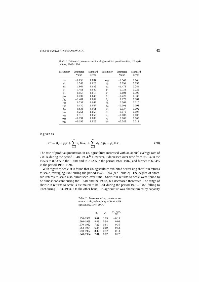
Table 1.Estimated parameters of translog restricted profit function, US agri-culture, 1948–1994.
Parameter Estimated Standard Parameter Estimated StandardValue Error Value Error
α0 −0.050 0.004 α22 −0.547 0.046β1 1.343 0.026 β3 0.094 0.058β2 1.664 0.032 β4 −1.479 0.284α1 −1.451 0.040 γ1 −0.738 0.222α2 −0.557 0.017 γ2 −0.104 0.305β11 0.732 0.045 δ1 −0.428 0.333β12 −1.401 0.064 δ2 1.270 0.184γ11 0.239 0.063 β5 0.062 0.010γ12 0.430 0.047 β6 −0.001 0.001β22 0.833 0.061 ϑ1 −0.037 0.002γ21 0.251 0.050 ϑ2 −0.019 0.003γ22 0.316 0.052 ε1 −0.008 0.005α11 −0.291 0.088 ε2 0.065 0.005α12 −0.199 0.026 β7 −0.048 0.011
is given as
πst = β5+ β6t +
n∑i=1
εi lnwi +m∑
j=1
ϑj ln pj + β7 ln z. (28)
The rate of profit augmentation in US agriculture increased with an annual average rate of7.81% during the period 1948–1994.12 However, it decreased over time from 9.01% in the1950s to 8.83% in the 1960s and to 7.22% in the period 1970–1982, and further to 6.34%in the period 1983–1994.
With regard to scale, it is found that US agriculture exhibited decreasing short-run returnsto scale, averaging 0.87 during the period 1948–1994 (see Table 2). The degree of short-run returns to scale also diminished over time. Short-run returns to scale were found tobe almost constant during the 1950s and the 1960s, but decreased thereafter. The range ofshort-run returns to scale is estimated to be 0.81 during the period 1970–1982, falling to0.69 during 1983–1994. On the other hand, US agriculture was characterized by capacity
Table 2. Measures ofπt , short-run re-turns to scale, and capacity utilization USagriculture, 1948–1994.
πt ρz(rk−vk)zk
TCs
1950–1959 9.01 1.03 −0.131960–1969 8.83 0.98 0.081970–1982 7.22 0.81 0.351983–1994 6.34 0.69 0.531950–1982 8.32 0.92 0.131948–1994 7.81 0.87 0.22
44 KARAGIANNIS AND MERGOS
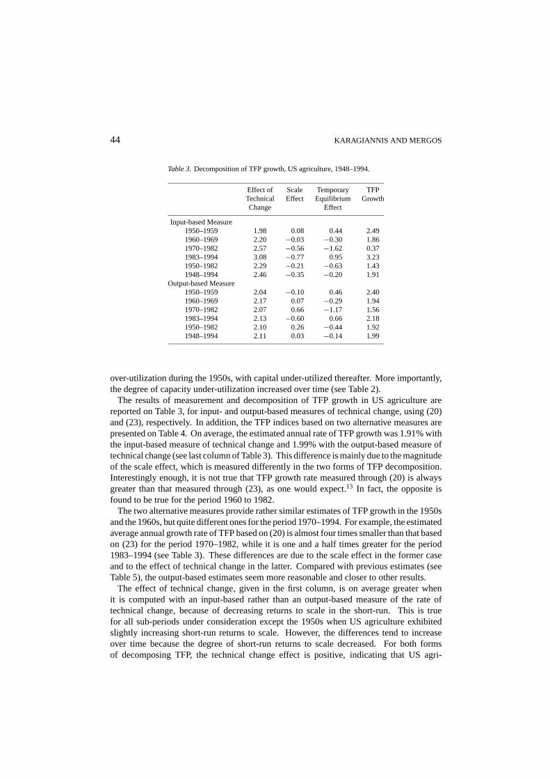
Table 3.Decomposition of TFP growth, US agriculture, 1948–1994.
Effect of Scale Temporary TFPTechnical Effect Equilibrium GrowthChange Effect
Input-based Measure1950–1959 1.98 0.08 0.44 2.491960–1969 2.20 −0.03 −0.30 1.861970–1982 2.57 −0.56 −1.62 0.371983–1994 3.08 −0.77 0.95 3.231950–1982 2.29 −0.21 −0.63 1.431948–1994 2.46 −0.35 −0.20 1.91
Output-based Measure1950–1959 2.04 −0.10 0.46 2.401960–1969 2.17 0.07 −0.29 1.941970–1982 2.07 0.66 −1.17 1.561983–1994 2.13 −0.60 0.66 2.181950–1982 2.10 0.26 −0.44 1.921948–1994 2.11 0.03 −0.14 1.99
over-utilization during the 1950s, with capital under-utilized thereafter. More importantly,the degree of capacity under-utilization increased over time (see Table 2).
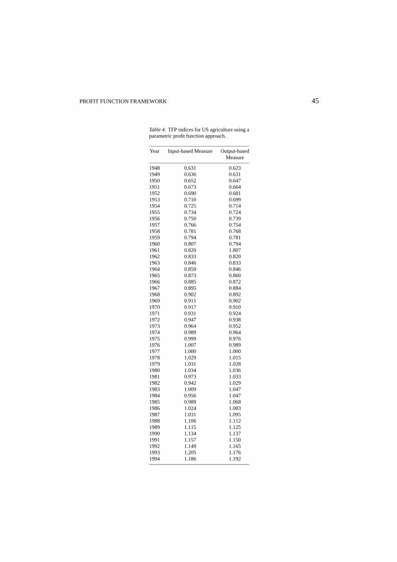
The results of measurement and decomposition of TFP growth in US agriculture arereported on Table 3, for input- and output-based measures of technical change, using (20)and (23), respectively. In addition, the TFP indices based on two alternative measures arepresented on Table 4. On average, the estimated annual rate of TFP growth was 1.91% withthe input-based measure of technical change and 1.99% with the output-based measure oftechnical change (see last column of Table 3). This difference is mainly due to the magnitudeof the scale effect, which is measured differently in the two forms of TFP decomposition.Interestingly enough, it is not true that TFP growth rate measured through (20) is alwaysgreater than that measured through (23), as one would expect.13 In fact, the opposite isfound to be true for the period 1960 to 1982.
The two alternative measures provide rather similar estimates of TFP growth in the 1950sand the 1960s, but quite different ones for the period 1970–1994. For example, the estimatedaverage annual growth rate of TFP based on (20) is almost four times smaller than that basedon (23) for the period 1970–1982, while it is one and a half times greater for the period1983–1994 (see Table 3). These differences are due to the scale effect in the former caseand to the effect of technical change in the latter. Compared with previous estimates (seeTable 5), the output-based estimates seem more reasonable and closer to other results.
The effect of technical change, given in the first column, is on average greater whenit is computed with an input-based rather than an output-based measure of the rate oftechnical change, because of decreasing returns to scale in the short-run. This is truefor all sub-periods under consideration except the 1950s when US agriculture exhibitedslightly increasing short-run returns to scale. However, the differences tend to increaseover time because the degree of short-run returns to scale decreased. For both formsof decomposing TFP, the technical change effect is positive, indicating that US agri-
PROFIT FUNCTION FRAMEWORK 45
Table 4.TFP indices for US agriculture using aparametric profit function approach.
Year Input-based Measure Output-basedMeasure
1948 0.631 0.6231949 0.636 0.6311950 0.652 0.6471951 0.673 0.6641952 0.690 0.6811953 0.710 0.6991954 0.725 0.7141955 0.734 0.7241956 0.750 0.7391957 0.766 0.7541958 0.781 0.7681959 0.794 0.7811960 0.807 0.7941961 0.820 1.8071962 0.833 0.8201963 0.846 0.8331964 0.859 0.8461965 0.873 0.8601966 0.885 0.8721967 0.895 0.8841968 0.902 0.8921969 0.911 0.9021970 0.917 0.9101971 0.931 0.9241972 0.947 0.9381973 0.964 0.9521974 0.989 0.9641975 0.999 0.9761976 1.007 0.9891977 1.000 1.0001978 1.029 1.0151979 1.031 1.0281980 1.034 1.0361981 0.973 1.0331982 0.942 1.0291983 1.009 1.0471984 0.956 1.0471985 0.989 1.0681986 1.024 1.0831987 1.031 1.0951988 1.106 1.1121989 1.115 1.1251990 1.134 1.1371991 1.157 1.1501992 1.149 1.1651993 1.205 1.1761994 1.186 1.192
46 KARAGIANNIS AND MERGOS
Table 5.Comparison of TFP growth rate (%) measures for US agriculture, (average annual).
Study 1950–59 1960–69 1970–82 1983–94 1950–82 1948–94
Accounting Approach
Theil-Tornqvist IndexUSDA (I)1 2.02 1.42
(II)2 1.47Ball (1985) 2.59 1.65Capalbo (1988a) 1.37 1.16 2.26 1.56Jorgenson & Gollop (1992) 1.583
Lambert (1998) 1.12
Fisher IndexBall et al (1997) 1.87 2.22 1.97 2.57 2.02 1.94Lambert (1998) 1.17
Non-parametric Approach4
Cox & Chavas (1990) 2.48 1.84 2.49 1.795
Chavas & Cox (1992) (I)6 2.71 1.55 2.82 2.39(II)7 1.86 1.79 2.38 2.05
Chavas & Cox (1994) (I)8 1.82 1.47 1.74 1.69(II)9 2.13 1.69 1.96 1.94
Lambert (1998) (I)8 1.2210
(II)9 1.6710
Parametric Approach
Production FunctionCapalbo (1988b) 1.5011
Luh & Stefanou (1991) 1.26 1.22 1.90 1.50Luh & Stefanou (1993) 1.18 0.93 1.71 1.31
Cost FunctionCapalbo (1988a) 1.27
Profit FunctionPresent Study (I)8 2.49 1.86 0.37 3.23 1.43 1.91
(II)9 2.40 1.94 1.56 2.18 1.92 1.99
Notes:1 Reported in Ball (1985)2 Reported in Trueblood and Ruttan (1995)3 Refers to the period 1948–1985 and it is reported in Trueblood and Ruttan (1995)4 Calculated by the authors from published TFP indices in Cox and Chavas (1990) and
Chavas and Cox (1992, 1994)5 Refers to the period 1950–19836 Based on 30-year lag specification of R&D7 Based on 15-year lag specification of R&D8 Input-based measure9 Output-based measure
10 These are the outer bound estimates11 Refers to the period 1948–1982
PROFIT FUNCTION FRAMEWORK 47
culture exhibited progressive technical change. Also, in both cases, the largest portionof TFP growth is attributed to technical change. Nevertheless, the input-based mea-sure indicates a continuous increase in the rate of technical change, while the output-based measure shows a slowdown in the rate of technical change during the period 1970–1982.
Significant differences arise with respect to the scale effect, which is given in the secondcolumn of Table 3. Using the input-based measure of the rate of technical change, basedon (20), the scale effect is, on average, negative while with the output-based measure ofthe rate of technical change, using (23), it is on average positive, albeit very small. Thesedifferences are due to different definitions of the scale effect in the two forms of decompo-sition. Nevertheless, in both (20) and (23), the magnitude of the scale effect is smaller andrelatively less significant compared to the technical change effect.
The magnitude and the sign of the temporary equilibrium effect is rather similar in thetwo measures (see Table 3). The capacity utilization of the quasi-fixed input (capital)had a generally negative contribution to TFP growth in US agriculture. Given that theweighted sum of variable and quasi-fixed inputs decreased over time, the sign of the tem-porary equilibrium effect indicates that, on average, the rental price of capital was greaterthan its shadow price, implying that capital was under-utilized during the period 1948–1994.
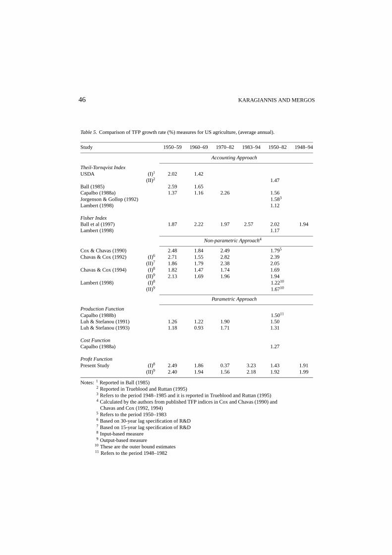
A comparison of the results reported in Table 3 with those of previous studies concerningmeasurement of TFP growth in US agriculture is given in Table 5.14 The results of thepresent study show interesting differences from he results of earlier studies using othermeasurement and decomposition methods. The result of the present study conform broadlywith those of Ballet al. (1997), who used a Fisher TFP index and found strong TFP growthrates in the 1950s and 1960s and a decline in TFP growth in the 1970s. Our results,however, are sharply different than those of Capalbo (1988), who utilized a Theil-TornqvistTFP index, and Luh and Stefanou (1991, 1993), who used a primal approach. Luh andStefanou (1991, 1993) found much lower TFP growth rates in the 1950s and 1960s and anacceleration of TFP growth in the 1970s.
A more direct comparison can be carried with Chavas and Cox (1994), who reportedprimal input- and output-based measures of TFP growth in US agriculture during the period1950–1982, using non-parametric techniques and assuming long-run equilibrium. Ourestimate of the average annual TFP during the same period is slightly lower (see Table 5).This is explained by the fact that the contribution of the temporary equilibrium effect isnegative. In both cases, however, the output-based measure is greater than the input-basedmeasure, indicating decreasing returns to scale.
5. Concluding Remarks
This paper develops a theoretical framework for measurement and decomposition of TFPgrowth using a profit function framework. Within the proposed framework, estimates ofTFP growth and identification of its sources are obtained by using directly the estimatedparameters of a profit function. The proposed framework offers two alternative estimates
48 KARAGIANNIS AND MERGOS
of TFP growth based on the output- and the input-based measures of the rate of technicalchange. It encompasses previous developments proposed by Bernstein (1994), who used ameasure of TFP growth that is similar, but apparently not the same, with the one developedin the presence of the input-based measure of the rate of technical change. The paperalso shows clearly the relation of the two alternative measures of the rate of technicalchange and makes them directly comparable, deriving both forms of TFP measurement anddecomposition using he same methodology.
A quantitative illustration of the results is presented by estimating a translog restrictedprofit function for US agriculture using published data for the period 1948–1994. Theresults of TFP measurement and decomposition based on two alternative measures of therate of technical change are very interesting. Although the average TFP growth rates for theentire period are very similar (1.91% and 1.99% in the cases of the input- and the output-based measures of the rate of technical changes), the rates for various sub-periods are quitedifferent. For example, for the period 1970–1982 not only is the average TFP growth ratedifferent (0.37% and 1.56% in the cases of the input- and the output-based measures ofthe rate of technical changes), but there are also other differences, such as in the sign ofthe scale effect. It seems that the difference is mainly due to the scale effect, while theeffect of technical change differs less and the temporary equilibrium effect is similar inboth cases.
Acknowledgments
Earlier versions of this paper has greatly benefited from the comments of C. J. MorrisonPaul, two anonymous reviewers and the participants of the 5th European Workshop onProductivity and Efficiency.
Notes
1. However, there have been some studies following a primal approach for decomposing TFP changes, such asBerndt and Fuss (1986), Bauer (1990), and Lovell (1996).
2. Agriculture is also a highly competitive industry and farmers’ objective is best described by profit maximizationas long as there are no production quotas. For the U.S. agriculture in particular, profit maximization is acommonly employed behavioral assumption; see Weaver (1983), Shumway (1983), Antle (1984), Ball (1988),Huffman and Evenson (1989), Luh and Stefanou (1991, 1993), among others.
3. There are advantages of using a profit function in estimating multiproduct technologies for price-taking firmsbecause inconsistencies in the econometric estimation due to simultaneous equation problems are avoided, asno endogenous variables (output or input levels) are used as explanatory variables (Lopez, 1982).
4. In particular, if observed output falls to the left of the minimum point of the long-run average cost curve,increasing short-run returns to scale may be associated with either under- or over-utilization, while decreasingshort-run returns to scale imply over-utilization. In contrast, if observed output falls to the right of the minimumpoint of the long-run average cost curve, increasing short-run returns to scale imply under-utilization, whiledecreasing short-run returns to scale may be associated with either under- or over-utilization.
PROFIT FUNCTION FRAMEWORK 49
5. In the case of profit function, it is not as straightforward as in the case of cost function (see Morrison,1986) to derive a relationship between short- and long-run returns to scale. The long-run profit maximiza-tion problem with all inputs variable need not result in the same optimal output bundle as the one derivedfrom the short-run problem, where some of the inputs are restricted to be quasi-fixed. Nevertheless, one canfind the optimal long-run stock of quasi-fixed inputs through the derivative propertyMk = ∂ lnπs/∂ ln zk
and then substitute it into short-run output supply and factor demand functions to derive their long-runcounterparts. Sometimes this becomes quite complicated as for example in the case of translog profitfunction, where a numerical solution is required to derive the optimal (long-run) level of quasi-fixed in-puts. By using (1) and (3),ρ = ρz + (
∑∂ lnπ/∂ ln pj )
−1 − (∑
∂ lnπs(p, w, z(p, w))/∂ ln pj )−1 +∑
Mk(p, w, z(p, w))/∑
Rj (p, w, z(p, w)) = ρz +∑
Mk(p, w, z(p, w))/∑
Rj (p, w, z(p, w)). Wewould like to thank C. Morrison and one reviewer for raising this point.
6. Graphically and in terms of a production function, the output-based measure of the rate of technical change ismeasured vertically. Thus, it shows the rate of output increase, due to a shift in production surface, by usingthe same amount of inputs as before. In contrast, the input-based measure of the rate of technical change ismeasured horizontally and indicates the amount of potential input saving for producing the same amount ofoutput as before, but operating at the new production function.
7. The following analysis is developed in the absence of adjustment cost, but it can be extended into a fullydynamic framework.
8. The distinction between input- and output-based decomposition of TFP growth in a profit framework is alsoimportant in the presence of productive inefficiency. For a theoretically consistent decomposition of TFPchange in such a case, the former should be associated with an input-based measure of technical inefficiencyand the latter with an output-based measure. For a derivation of input- and output-based measure of productive(technical and allocative) inefficiency within a primal and a profit function see Kumbhakar (1996).
9. The profit function (36) and the profit share equation of livestock were corrected for third-order autocorrelationby using a Cochrani-Orcutt procedure, while the profit share equation of labor was corrected for first-orderautocorrelation.
10. This is equivalent to positive semi-definiteness of the modified Hessian (Antle and Capalbo, 1988). Thedeterminants of the principal minors of the modified Hessian areH1 = 1.193, H2 = 1.617, H3 = 1.237 andH4 = 0.332 and its eigenvalues 0.0005, 0.1918, 0.7222, and 5.8014.
11. At the point of approximation, the determinants of the principal minors of the Hessian matrix correspondingto quasi-fixed factor are found to be 0.094 and−1.479.
12. Diewert’s (1976) quadratic approximation lemma is used to convert the continuous time model developed inthe second and third section to discrete variables calculations used in the fourth section.
13. In absolute terms however the input-based TFP index is greater than the output-based index during the period1948–1980, while the opposite is true for the rest of the period under consideration (see Table 4).
14. A comparison of the explanatory power of different approaches used to measure TFP in US agriculture is notalways possible because in the studies using the primal approach to decompose the growth in TFP (e.g., Luhand Stefanou, 1991, 1993) the rate of technical change is calculated as a residual. A comparison may howeverbe possible with Capalbo (1988a) parametric cost function approach regarding the period 1950–1982. In thecase of cost function, the unexplained residual is 18.6%, while in the case of profit function is 8.3% and 23.1%for the output- and the input-based measures of TFP growth, during the same period.
References
Antle, J. M. (1984). “The Structure of U.S. Agricultural Technology, 1910–1978.”American Journal of Agricul-tural Economics66, 414–21.
Antle, J. M. and S. M. Capalbo. (1988). “An Introduction to Recent Developments in Production Theory andProductivity Measurement.” In S. M. Capalbo and J. M. Antle (eds.),Agricultural Productivity: Measurementand Explanation. Washington D.C.: Resource for the Future.
Ball, V. E. (1985). “Output, Input and Productivity Measurement in U.S. Agriculture.”American Journal ofAgricultural Economics67, 475–86.
Ball, V. E. (1988). “Modeling Supply Response in a Multiproduct Framework.”American Journal of AgriculturalEconomics70, 813–25.
50 KARAGIANNIS AND MERGOS
Ball, V. E., J. C. Bureau, R. Nehring, and A. Somwaru. (1997). “Agricultural Productivity Revisited.”AmericanJournal of Agricultural Economics79, 1045–63.
Bauer, P. W. (1990). “Decomposing TFP Growth in the Presence of Cost Inefficiency, Nonconstant Returns toScale, and Technological Progress.”Journal of Productivity Analysis1, 287–299.
Berndt, E. R. and M. A. Fuss. (1986). “Productivity Measurement with Adjustments for Variation in CapacityUtilization and Other Forms of Temporary Equilibrium.”Journal of Econometrics33, 7–29.
Bernstein, J. I. (1994). “Exports, Margins and Productivity Growth: With an Application to the Canadian SoftwoodLumber Industry.”Review of Economics and Statistics76, 291–301.
Callan, S. J. (1991). “The Sensitivity of Productivity Growth Measures to Alternative Structural and BehavioralAssumptions: An Application to Electric Utilities, 1981–1984.”Journal of Business and Economic Statistics9, 207–13.
Capalbo, S. M. (1988a). “Measuring the Components of Aggregate Productivity Growth in U.S. Agriculture.”Western Journal of Agricultural Economics13, 53–62.
Capalbo, S. M. (1988b). “A Comparison of Econometric Models of U.S. Agricultural Productivity and AggregateTechnology.” In S. M. Capalbo and J. M. Antle (eds.),Agricultural Productivity: Measurement and Explanation.Washington D.C.: Resource for the Future.
Caves, D. W., L. R. Christensen, and J. A. Swanson. (1981). “Productivity Growth, Scale Economies, andCapacity Utilization in U.S. Railroads, 1955–74.”American Economic Review71, 994–1002.
Caves, D. W., L. R. Christensen, and W. E. Diewert. (1982). “The Economic Theory of Index Numbers and theMeasurement of Input, Output and Productivity.”Econometrica50, 1393–1414.
Chavas, J. P. and T. L. Cox. (1992). “A Nonparametric Analysis of the Influence of Research on AgriculturalProductivity.” American Journal of Agricultural Economics74, 583–91.
Chavas, J. P. and T. L. Cox. (1994) “A Primal-Dual Approach to Nonparametric Productivity Analysis: The Caseof U.S. Agriculture.”Journal of Productivity Analysis5, 359–73.
Coelli, T. J. (1996). “Measurement of Total Factor Productivity Growth and Biases in Technological Change inWestern Australian Agriculture.”Journal of Applied Econometrics11, 77–91.
Cox, T. L. and J. P. Chavas. (1990). “A Nonparametric Analysis of Productivity: The Case of U.S. Agriculture.”European Review of Agricultural Economics17, 449–64.
Denny, M., M. Fuss, and L. Waverman. (1981). “The Measurement and Interpretation of Total Factor Productivityin Regulated Industries: An Application to Canadian Telecommunications.” In T. Cowing and R. Stevenson(eds.),Productivity Measurement in Regulated Industries. N.Y.: Academic Press.
Diewert, W. E. (1973). “Functional Forms for Profit and Transformation Functions.”Journal of Economic Theory6, 284–316.
Diewert, W. E. (1976). “Exact and Superlative Index Numbers.”Journal of Econometrics4, 115–45.Fousekis, P. and A. Papakonstantinou. (1997). “Economic Capacity Utilization and Productivity Growth in Greek
Agriculture.” Journal of Agricultural Economics48, 38–51.Fox, K. J. (1996). “Specification of Functional Form and the Estimation of Technical Progress.”Applied Economics
28, 947–56.Granderson, G. (1997). “Parametric Analysis of Cost Inefficiency and the Decomposition of Productivity Growth
for Regulated Firms.”Applied Economics29, 339–48.Huffman, W. E. and R. E. Evenson. (1989). “Supply and Demand Functions for Multiproduct U.S. Cash Grain
Farms: Biases Caused by Research and Other Policies.”American Journal of Agricultural Economics71,761–73.
Hulten, C. R. (1978). “Growth Accounting with Intermediate Inputs.”Review of Economic Studies45, 511–18.Hulten, C. R. (1986). “Productivity Change, Capacity Utilization and the Sources of Efficiency Growth.”Journal
of Econometrics33, 31–50.Jayne, T. S., Y. Khatri, C. Thirtle, and T. Reardon. (1994). “Determinants of Productivity Change using a Profit
Function: Smallholder Agriculture in Zimbabwe.”American Journal of Agricultural Economics76, 613–18.Jorgenson, D. W. and F. M. Gollop. (1992). “Productivity Growth in U.S. Agriculture: A Postwar Perspective.”
American Journal of Agricultural Economics75, 745–50.Judge, G. G., W. E. Griffiths, R. Carter Hill, and T. S. Lee. (1980).The Theory and Practice of Econometrics.
N.Y.: Wiley & sons.Kumbhakar, S. C. (1996). “Efficiency Measurement with Multiple Outputs and Multiple Inputs.”Journal of
Productivity Analysis7, 225–55.Lambert, D. K. (1998). “Productivity Measurement from a Reference Technology: A Distance Function Ap-
proach.”Journal of Productivity Analysis10, 289–304.
PROFIT FUNCTION FRAMEWORK 51
Levy, V. (1981). “Total Factor Productivity, Non-neutral Technical Change and Economic Growth.”Journal ofDevelopment Economics8, 93–109.
Lopez, R. E. (1982). “Applications of Duality Theory to Agriculture.”Western Journal of Agricultural Economics7, 353–65.
Lovell, C. A. K. (1996). “Applying Efficiency Measurement Techniques to the Measurement of ProductivityChange.”Journal of Productivity Analysis7, 329–40.
Luh, Y. H. and S. E. Stefanou. (1991). “Productivity Growth in US Agriculture under Dynamic Adjustment.”American Journal of Agricultural Economics73, 1116–125.
Luh, Y. H. and S. E. Stefanou. (1993). “Learning-By-Doing and the Sources of Productivity Growth: A DynamicModel with Application to US Agriculture.”Journal of Productivity Analysis4, 353–70.
Lynde, C. and J. Richmond. (1993). “Public Capital and Total Factor Productivity.”International EconomicReview34, 401–14.
Morrison, C. J. (1986). “Productivity Measurement with Non-static Expectations and Varying Capacity Utilization:An Integrated Approach.”Journal of Econometrics33, 51–74.
Morrison, C. J. (1992). “Unraveling the Productivity Growth Slowdown in the United States, Canada and Japan:The Effects of Subequilibrium, Scale Economies and Markups.”Review of Economics and Statistics74, 381–93.
Morrison Paul, C. J. (1999). “Scale Economy Measures and Subequilibrium Impacts.”Journal of ProductivityAnalysis11, 55–66.
Nadiri, M. I. and I. R. Prucha. (1990). “Dynamic Factor Demand Models, Productivity Measurement, and Rates ofReturn: Theory and an Empirical Application to US Bell System.”Structural Change and Economic Dynamics1, 263–89.
Ohta, M. (1974). “A Note on the Duality between Production and Cost Functions: Rate of Returns to Scale andRate of Technical Change.”Economic Studies Quarterly25, 63–65.
Ray, S. C. and K. Segerson. (1991). “A Profit Function Approach to Measuring Productivity Growth: The Caseof US Manufacturing.”Journal of Productivity Analysis2, 39–52.
Shumway, R. C. (1983). “Supply, Demand, and Technology in a Multiproduct Industry: Texas Field Crops.”American Journal of Agricultural Economics65, 45–56.
Solow, R. (1957). “Technical Change and the Aggregate Production Function.”Review of Economics and Statistics39, 312–20.
Trueblood, M. A. and V. W. Ruttan. (1995). “A Comparison of Multifactor Productivity Calculations of the U.S.Agricultural Sector.”Journal of Productivity Analysis6, 321–31.
Weaver, R. (1983). “Multi-input, Multi-output Production Choices and Technology in the U.S. Wheat Region.”American Journal of Agricultural Economics65, 45–56.