Embed Size (px)
Citation preview

TOURISM AND THE CURRENT ACCOUNT POSITION IN KENYA
OMONDI EDGAR OWINO
X51/79380/2012
A RESEARCH PAPER SUBMITTED TO THE UNIVERSITY OF
NAIROBI, SCHOOL OF ECONOMICS, IN PARTIAL FULFILMENT
OF THE REQUREMENTS FOR THE AWARD OF MASTERS OF
ARTS DEGREE IN ECONOMIC POLICY MANAGEMENT
OCTOBER 2014

ii
DECLARATION
I hereby declare that this is my original work and that to the best of my knowledge has
never been presented for the award of any degree in any other university or institution.
CANDIDATE: EDGAR OMONDI OWINO
ADMISSION NUMBER: X51/79380/2012
SIGNATURE: ……………………………………….DATE:………………………
APPROVAL
This MA Thesis has been forwarded for examination with our approval as university
supervisors:
DR. OSORO KENNEDY
SIGNATURE: ……………………………………….DATE:………………………
PROF: MANDA KULUNDU
SIGNATURE: ……………………………………….DATE:………………………

iii
DEDICATION
I dedicate this work to my family for their firm support in encouraging and reminding me
of the value of time for period I was undertaking my studies. There positive advice and
commitment ensured my accomplishing of this work. They are much appreciated.

iv
ACKNOWLEDGEMENT
I take this opportunity to express my profound gratitude and deep regards to my
supervisors Dr. Osoro Kennedy and Prof. Kulundu Manda for their exemplary guidance,
monitoring and constant encouragement throughout the course of this research project.
The blessing, help and guidance given by them, time to time shall carry me a long way in
the journey of life on which I am about to embark.
I also take this opportunity to express a deep sense of gratitude to University of Nairobi
school of Economics for their cordial support, valuable information and guidance, which
helped me in completing this task through various stages.
I am obliged to my class mates, for the valuable information provided by them in their
respective fields. I am grateful for their cooperation during the period of my assignment.
Lastly, I thank almighty, my parents, brothers, sister and friends for their constant
encouragement without which this assignment would not be possible.
Thank you
v
LIST OF FIGURES
Figure 1: Trend of current account in Kenya ( Kshs Billion) (1980-2013) ...................4
Figure 2: Trend of tourism earnings in Kenya ( Kshs Billion) (1980-2013) ...................8

vi
LIST OF TABLES
Table 1: Summary of descriptive Statistics ......................................................................34
Table 2: Stationarity test at Level and first difference ......................................................35
Table 3: Unrestricted cointergrating rank Test (Trace Test)..............................................36
Table 4: Lag length Selection Criterion .............................................................................37
Table 5: Vector error correction model (VECM) ..............................................................38
Table 6: Granger causality .................................................................................................39
Table 7: Regression Analysis ............................................................................................40

vii
LIST OF APPENDICIES
Appendix 1 : Unit Root Test at Level ................................................................................49
Appendix 2 : Unit Root Test at First Difference ................................................................49
Appendix 3 : Cointergration test ........................................................................................50
Appendix 4 : Selection Order Criteria ...............................................................................50
Appendix 5 : Vector Error Correction Model ....................................................................51
Appendix 6 : Johansen Normalization Restriction ...........................................................52
Appendix 7 : Granger Causality Test ...............................................................................53
Appendix 8 : Regression Analysis .....................................................................................54
Appendix 9 : Serial Correlation Test .................................................................................54

viii
LIST OF ACRONYMS AND ABBREVIATIONS
ADF - Augmented Dickey –Fuller
BOM - Balance on Merchandise
BOT - Balance of Trade
CAD - Current Account Deficit
CT - Current Transfer
FEX - Foreign Exchange Rate
GDP -Gross Domestic Product
KNBS - Kenya National Bureau of Statistics
OLS -Ordinary Least Squares
TOURE - Tourism Earnings
UNWTO - United Nations World Tourism Organization
VAR - Vector Autoregressive Regression
VECM - Vector Error Correction Model
WTO -World Tourism Organization
Y - Income Per Capita
ix
TABLE OF CONTENTS
DECLARATION ............................................................................................................................. ii
DEDICATION ................................................................................................................................ iii
LIST OF FIGURES ......................................................................................................................... v
LIST OF TABLES .......................................................................................................................... vi
LIST OF APPENDICIES ............................................................................................................... vii
LIST OF ACRONYMS AND ABBREVIATIONS ....................................................................... viii
TABLE OF CONTENTS .................................................................................................................ix
ABSTRACT .................................................................................................................................... xii
CHAPTER ONE : INTRODUCTION ............................................................................................. 1
1.1 Background ......................................................................................................................... 1
1.1.1 Kenya Current Account Position ........................................................................................ 4
1.2.1 Tourism in Kenya .............................................................................................................. 7
1.2 Statement of the Problem .................................................................................................. 10
1.3 General Objective ............................................................................................................. 11
1.3.1 Specific Objective ............................................................................................................. 11
1.4 Research Questions ........................................................................................................... 11
1.5 Justification and Significance of the Study ....................................................................... 12
CHAPTER TWO : LITERATURE REVIEW ............................................................................... 13
2.0 Introduction ....................................................................................................................... 13
2.1 Theoretical Literature Review .......................................................................................... 13
2.2.1 Elasticity Approach to Current Account ........................................................................... 13
2.2.2 Marshall – Lerner Condition ............................................................................................. 14
2.2.4 Absorption Approach to Current Account ........................................................................ 15
2.2.5 Inter-Temporal Approach to Current Account.................................................................. 15

x
2.2.6 Monetary Approach to Current Account .......................................................................... 16
2.3 Empirical Literature Review ............................................................................................. 16
2.4 Overview of the Literature ................................................................................................ 21
CHAPTER THREE : METHODOLOGY ..................................................................................... 24
3.0 Introduction ....................................................................................................................... 24
3.2.1 Model Specification .......................................................................................................... 24
3.2.2 Theoretical Framework ..................................................................................................... 24
3.3 Definition, Measurement of Variables and Expected Results .......................................... 27
3.3.1 Current Account ................................................................................................................ 27
3.3.2 International Tourism Earnings (Balance on Service) ...................................................... 27
3.3.3 Balance on Merchandise Trade ......................................................................................... 28
3.3.4 Foreign Exchange Rate ..................................................................................................... 28
3.3.5 Current Transfers .............................................................................................................. 29
3.3.7 Income Per-Capita ............................................................................................................ 29
3.4 Data Type and Source ...................................................................................................... 30
3.5 Estimation Techniques ...................................................................................................... 30
3.6 Statistical Tests ................................................................................................................. 31
3.6.1 Unit Root and Stationarity Test ........................................................................................ 31
3.6.2 Cointergration Test ........................................................................................................... 31
3.6.3 Vector Error Correction Model ......................................................................................... 31
3.6.4 Granger Causality ............................................................................................................. 32
3.6.5 Diagnostics Tests For Normality And Serial Correlation ................................................. 32
CHAPTER FOUR : EMPIRICAL FINDINGS AND DISCUSSION ........................................... 34
4.1 Descriptive Statistics ......................................................................................................... 34
4.2 Unit root test and results ................................................................................................... 35
4.2 Cointergraton Test Results and Vector Error Correction Model ...................................... 36

xi
4.3 Granger Causality ............................................................................................................. 39
4.4 Regression Results ............................................................................................................ 40
4.5 Discussion of the Estimation Results ................................................................................ 41
CHAPTER FIVE : CONCLUSION AND POLICY OPTIONS .................................................... 43
5.1 Conclusion ........................................................................................................................ 43
5.2 Policy Options................................................................................................................... 44
5.3 Area for future research .................................................................................................... 45
6.0 REFERENCES ................................................................................................................. 46
APPENDICIES .............................................................................................................................. 49

xii
ABSTRACT
This study aimed at investigating the existence of a long run relationship between tourism
earnings and current account position by examining the effect of tourism earnings on
current account deficit in Kenya. The study further determined factors that affect current
account in Kenya. The study employed cointergration and vector error correction model
and regression analysis. The findings of the study revealed that tourism earnings had a
positive coefficient as predicted and was in conformity with previous related studies
conducted on relationship between tourism and current account balance. It was also
revealed that tourism earnings were not statistically significant to explain changes in the
current account even though it exhibited characteristics of a long run relationship with
current account deficit. The possible reason for tourism not being statistically significant
is due to the data used in the analysis. The study further established that balance on
merchandise was the major contributor to the persistent deficit and was statistically
significant to explain variation in the current account deficit in Kenya. The study
concluded that for Kenya government to control and reduce the persistent current account
deficit there is needed to apply fiscal policies and vision 2030 strategies and this was
driven by the fact that the imports in Kenya are higher than export creating the huge gap
which contribute to the deficit in balance on merchandise.

xiii

CHAPTER ONE
INTRODUCTION
1.1 Background
Trade between countries is an essential ingredient in the economic prosperity of any
country. With increasing globalization, countries become more and more intertwined in
their economic lives. This trade takes different forms but with the intended purpose of
allowing each trading nation the benefit of accessing goods and services from trading
partners. One of the products that are increasingly traded at the international market is
tourism. It has gained considerable importance in the global economy, both for developed
and developing countries like Kenya. From direct and indirect combined activities, the
travel and tourism sector accounted for a remarkable 4.8% of world export and 9.2% of
world’s investment UNWTO (2010).
All these economic activities traded among countries are recorded in an official account
known as balance of payment. Balance of payment is a statistical statement that
aggregates up all transactions that occur between residents and non-residents of a nation.
These transactions incorporates things such as stock of exports and imports, tourism
earnings, government securities and purchase of financial and real assets abroad, stock,
real estates and government bonds. These transactions are recorded within a specific
period of time. It is this transactions that offer ascent to sets of accounts that demonstrates
all the stream of worth between inhabitant of one nation and inhabitants of different
nations when they enter into financial transactions. The balance of payment comprise
three accounts, the current account which contains the visible and invisible transactions,

2
the capital account which outlines the purchasing and selling of assets among nations and
the financial account which records the foreign reserve of a nation. Balance of payment
thus is a bookkeeping framework that economist apply to break down the net impact of
exchanging values between nations. It is an account which is critical in showing the
strength of an economy and as a source of intelligence for foreign creditors on the credit
worthiness of a country.
Transactions recorded in the statement of account follow a systematic manner of double
entry rule, where it gives an overall net balance of zero since each transaction within the
system requires an offsetting of credit and debit entry. In other words the transactions of a
country signify if a country is a creditor or a debtor. Many developing countries including
Kenya have faced the challenges of being regarded as a debtor due to the impact of huge
and persistent current account deficit they are having. This has posed a threat to the
economic well-being of their nations.
The current account can be defined as the sum of trade balance , income balance and
transfer balance, when current account is divided by the gross domestic product of a
country and expressed in percentage is referred to as the current account as a percentage
of GDP. Over the last three decades developing countries have experienced current
account imbalances which have prompted economist and policy makers to center their
attention to the dynamics of current account balance. The current account can be further
measured as the difference between the value of exports of goods and services and the
total value of imports of goods and services. Current account imbalances can either be
two folds: surplus or deficit, A deficit means that the country is importing more goods

3
and services than it is exporting and vice versa for surplus. For a capital – poor
developing countries which is regarded as a market for more investment opportunities,
the current account can be termed as the difference between national savings and
investment where a deficit in this case reflects a low level of national savings relative to
investment or vice versa for surplus.
For Kenya as one of the developing nations has experienced a high export import gap due
to inelasticity of demand for its primary products from foreign markets, attraction to
foreign goods than locally produced and processed goods .This has aggravated the
pressure on the current account creating huge deficits.
One of the significant macroeconomic objectives of a nation is the attainment of the
external balance in an economy. This can be reflected by the current account position.
For a nation that experience current account deficit is an indication of poor performance
especially when it is in the form of large deficit (Fisher 1988). Kenya’s history of current
account deficit has shown persistent deficit hitting a record of 18.7% of GDP in 1998
and a decade high of 13.1% of GDP in 2012 (KNBS 2013). Attention has been focused
on current account since last surplus was recorded in 2003, because of the upward trend
in growth of the deficit which has continued unabated.
While current account deficit can be used as a barometer for measuring the underlying
investment finance gap that requires to be filled, it can paint a bad picture when it comes
to credit worthiness of a nation .This therefore necessitates an inquiry into the trend of
current account position in Kenya.

4
1.1.1 Kenya Current Account Position
Kenya’s current account has been in deficit for many years except in 1993, 1994 and
2003, for the period 1980-2012. The chart in figure 1 shows the trend of current account
deficit in Kenya over the period between 1980 and 2013.
Figure 1
Source: Kenya National Bureau of Statistics: Economic survey various
The first highest current account deficit occurred in 1980 of Kshs 6.66 Billion and was
caused by a severe drought combined with an oil shock which widened the Current
account deficit (KNBS 1981). In 1981-1985 the current account deficit improved from a
deficit of Kshs 5.06 Billion to Kshs 1.58 Billion which was attributed to the inflow of
capital from the rest of the world and to the invisible transaction improvement which
recorded a surplus of Kshs 5.52 Billion compared to Kshs 4.54 Billion in 1984
representing an increase of 22% (KNBS 1986). In the year 1986 there was a remarkable
improvement of Current account deficit due to large inflow of foreign exchange through

5
embassies, international bodies which led the external account to record a deficit of Kshs
0.62 Billion (KNBS 1987). The current account worsened to Kshs 8.13 Billion during
1987 and it was attributed to net earnings on services and the inflow of grants declining
(KNBS 1988). In the year 1988 there was improvement in the deficit which was brought
about by the invisible subsector where the earnings from tourism improved from a
surplus of Kshs 3.56 Billion to Kshs 5.86 Billion in 1988 and further boosted by inflow
of grants which doubled during the period (KNBS 1989). In 1989 current account deficit
worsened to Kshs 12.08 Billion compared to 1988 and this was due to deterioration in
adjusted merchandise transactions which came about due to the continued liberalization
of import licensing and weakening of Kenya shilling against the currencies of major
trading partners and export grew relatively slow (KNBS 1990). In the year 1990 to 1992
the current account realized an improvement which was attributed to good performance
by the transport and tourism sector of the economy and a remarkable increase in private
grants, where it moved from Kshs 10.88 Billion to Kshs 5.79 Billion in 1991 and further
improved due to the high earnings realized in the tourism sector (KNBS 1993).
The first surplus in current account was seen in 1993 where there was a record of Kshs
5.75 Billion. This surplus was due to good performance in the export and tourism sector,
improved inflow of short term capital and grants in addition to arrears on foreign debt
servicing (KNBS 1994). The surplus continued to be realized in the subsequent year
where there was a record of Kshs 5.82 Billion realized compared with what was realized
in 1993. There was a boost in surplus from the export of coffee, pyrethrum, horticultural
products and cement (KNBS 1995). While in 1995 to 1998 the deficit trend was back

6
again with a record of Kshs 20.61 Billion, Kshs 4.19 Billion, Kshs 22.15 Billion and
Kshs 24.50 Billion respectively in the years 1995, 1996, 1997 and 1998. This was
associated with widening trade deficit brought about by substantial increase in import
payment and a sluggish export performance (KNBS 1999).
Resumption of aid in the year 2000 improved the current account to a deficit of Kshs
15.18 Billion, which continued building up towards a surplus of Kshs 11.10 Billion in
2003 (KNBS 2004). After this surplus, the account continued to tumble to a point where
it hit 8% of the GDP in the subsequent years moving from a deficit of Kshs 10.85, Kshs
19.06, Kshs 36.80, Kshs 69.46 and Kshs 137.14 Billion in 2008. This was attributed to
the violence after the 2007 disputed elections which disrupted the production of food
crops. This was also followed by drought and world economic recession in 2008. As a
result the current account deficits increased, exchange rates depreciated and terms of
trade deteriorated. This affected the cost of production, and food imports thereby leading
to a drop in GDP (KNBS 2009). In 2009-2010 Kenya recorded a deficit of Kshs 124.44
Billion in the current account which was attributed to the effects of the world economic
slowdown and the depreciation of the shilling against the dollar.
On the other hand, the years 2011 was regarded as the most challenging in Kenya. The
country was faced with heavy expenditures in carrying out referendum, passing of the
new constitution and the implementation challenges, weather changes and the aftermath
of global economic recession of 2008. The current account faced therefore the challenges
of world economic slowdown, and Net official reserves declined due to growth in import
bill and there was unmatched growth in exports of goods and services. As a result Kenya

7
recorded a current account deficits of Kshs 359.67 Billion in 2012. A report by the Kenya
National Bureau of Statistics (KNBS 2014) showed the total current account deficit
worsened as a result of faster growth in the merchandise import bill to a deficit of Kshs
412.37 Billion in 2013 (KNBS 2014).
1.2.1 Tourism in Kenya
The tourism industry is one of the fastest developing sectors and adopted by many
developing countries as one of the most net worth source of economic prosperity.
Tourism earnings makes an important contribution to economies resulting to positive
effects such as job creation, additional income for private and public sector, foreign
currency receipt , higher investment and growth. (WTO 1994).
International tourism is treated to be a key source of export earnings where the consumer
moves instead of the product. Sinclair (2002) indicated in his study that tourism is a
complex product involving capital-intensive investments such as air transport,
infrastructure, accommodation, catering, entertainment and services such as curio shops
and currency exchange.
Powerful links exist between tourism and key economic sectors. It starts with Visitor
arrivals which has multiplier effects on the economy, in that it boosts economic activity
generated through the increase in visitor arrivals and expenditure. The immediate change
is seen in the increased revenues of firms involved in the tourism sector. It is this firms
who then purchase goods and services from other suppliers domestically and
internationally, thus causing an indirect effect. According to Sinclair, it is at the aggregate
level that the effect of visitor arrivals occurs on the current account. Revenue from

8
tourism on the other hand form a major item in the current account. Schubert and Brida
(2009) on the other hand linked tourism to current account through increase in arrival of
tourist. Their findings indicated a positive effect of visitor’s arrival on current account
deficit caused by increased foreign exchange reserves, increased exports and availability
of capital to imports.
Tourism over the last six decades has developed and diversified to becoming one of the
largest and fastest growing economic sector in the world. According to UNWTO tourism
barometer 2011, tourism arrival has grown tremendously by a growth rate of 5 percent
per annum, this consolidated trend has been seen in 2010, where the demand for
international tourism maintained a momentum. Arrivals grew from 943 million tourists in
2010 to 983 million tourist in 2011 and international receipt also increasing from 928
billion US dollars in 2010 to 1,030 billion US dollars in 2011 .Within Kenya, the success
of tourism was evident when the sector became the fastest growing and most important
sector of the Kenyan economy. The figure 2 shows the trend of international tourism
earnings over the period between 1980-2013.
Figure 2
Source World Tourism Organisation and UNWTO data (1980-2013)

9
From 1980 to 1988, international tourist arrivals in Kenya increased at an average of 10
% annually .Tourist arrivals expanded from 393,300 in 1980 to 781,600 in 1991. The
number of arrivals peaked in 1994, rose to 1,008,300 before declining to 973, 614 in
1995. Contrary to this downward trend, tourist arrivals world-wide totaled 561 million in
1995 reflecting a growth rate of 5.5% (WTO 1990). Tourism earnings increased more
than three times from Kshs 2.40 Billion in 1983 to Kshs 8.60 Billion in 1989, before
rising to Kshs 28.02 Billion Million in 1994. This was attributed to a number of factors
that included inflation and the fall in the value of Kenya shilling in relation to the US
dollar. From 1995 to 2000 tourism earnings dropped from Kshs 25.60 Billion to as low as
Kshs 17.50 Billion then regained to Kshs 21.60 Billion due to low tourist arrivals and
travel advisory. (KNBS 2001)
The tourism sector maintained an upward trend in 2001-2007, realizing a 13.6% growth
in 2007 in tourist arrivals compared with 8.2% in 2006. Earnings also maintained an
upward trend and increased by 28.9% in 2007 to record Kshs 65.40 Billion from Kshs
56.9 Billion the previous year (WTO 2008). In 2008-2010, net tourism earnings declined
and then shot up to a record of Kshs 73.70 Billion from Kshs 52.70 Billion in the year
2008. However, in 2008, the sector suffered a major blow as a result of the post-election
violence, increased oil prices and, the world economic crisis. (KNBS 2009). In 2009,
tourist arrivals declined by 33.9% and dollar earnings declined by 19.9% to record an
entry of Kshs 53.30 Billion. There was a big recovery in 2011, which suggested that the
tourism effect was owed to the post-election violence rather than the crisis where the
earning shot up to Kshs 97.90 Billion (WTO 2012).

10
During the year 2012 tourism earnings decreased from Kshs 97.90 Billion in 2011 to
Kshs 96.00 Billion in 2012. International visitors’ arrival decreased by 6.1 % from 1.8
million in 2011 to 1.70 million in 2012. This decline in performance was attributed by
slowdown in the global economy especially in the euro zone coupled with travel
advisories over securities concerns (WTO 2013). This dealt a major blow to tourism
sector and further deteriorated tourism earnings in 2013 to Kshs 94.00 Billion (KNBS
2014).
According to the World Bank (2012), Kenya’s current account deficit had hit a record of
13.7% of Gross Domestic Product (GDP), while its export import gap has widened to a
record of 20% of Import growth and 10% of export growth. The widening of this gap
brought about by import has been due to oil import which amounted to 27.6% of total
import bill in 2011, an increase by 2.7 from the previous year of 2010 which recorded
8.9% of GDP. Further the rise in world crude oil by 33%, increase in consumption
volume by 12% has further worsened the gap. That aside, the constant status of factors
such as Net factor income and Current transfer also have contributed to the worsening of
the current account deficit
1.2 Statement of the Problem
Tourism earnings play a significant role in enhancing current account position in the
balance of payment. It is a service that generates significant foreign exchange earnings
through tourism receipt from spending by tourists visiting the country. Kenya’s tourism
sector in general has recorded tremendous growth, where there has been an increase in
foreign exchange earnings from as low as Kshs 2.24 Billion in 1980s to as high as Kshs

11
94.00 Billion in 2013. Despite this undisputed growth of the sector, the current account
has persistently recorded huge deficits. Tourism being the second largest foreign
exchange earner after horticulture, then why is there a persistent current account deficit?
Understanding the link between tourism earnings and Current account deficit is therefore
critical in highlighting the direct effect of tourism earnings on Current account deficit and
in determining policy options that can improve outcomes relating to this linkage.
1.3 General Objective
The main objective of this research was to investigate the existence of a long run
relationship between tourism earnings and current account imbalances that have
occurred between 1980 and 2013 in Kenya using time series regression model.
1.3.1 Specific Objective
To determine the factors affecting Current account in Kenya.
To model the relationship between tourism earnings and Current account in
Kenya
To offer policy options based on research findings.
1.4 Research Questions
What are the factors affecting Current account in Kenya?
What is the relationship between tourism earnings and Current account in Kenya?
What is the policy option drawn from the study?

12
1.5 Justification and Significance of the Study
Studies on current account have to be undertaken since they assist in identification of key
components which affect the economy. However, most studies that have been undertaken
regarding current account have concentrated on key determinants in current account. This
has prompted this study in investigating the effect of tourism on current account, since
tourism is regarded as a factor that can trigger growth in the economy and has been
embraced by many developing countries.
However, very little has been done to establish the link between current account and
tourism given that this is a variable that contribute foreign exchange earnings in terms of
export of service
I believe this research can be helpful to the nation and development of the low income
countries such as Kenya which aims to be industrialized by the year 2030 through its blue
print Vision 2030 where tourism has been factored as a sector responsible for boosting
economic performance.

13
CHAPTER TWO
LITERATURE REVIEW
2.0 Introduction
The persistent current account deficit is a major challenge in developing nations that is
hindering economic improvement, and there exist no single solution that can solve the
problem of current account deficit. This has further been aggravated by the different and
unique structure that developing countries pursue and moreover the causes of the
persistent current account deficit. The first section of this chapter shows various theories
that have been developed on ways of correcting the current account deficit problem,
while the second section entails, studies that have been conducted by various authors on
current account and tourism, methods they have adopted and conclusion of their findings,
while the last section of the chapter looks at the overview of the entire chapter
2.1 Theoretical Literature Review
2.2.1 Elasticity Approach to Current Account
This is an approach proposed by (Metzler 1948). Elasticity Approach suggests that
current account deficit arise due to excess demand for foreign exchange. It is an approach
that assumes prices are flexible and that income is fixed. It explains Current account
deficit in terms of prices and that prices are responsible in creation of a trade balance.
The authors regard prices to be the exchange rate. According to this approach, where
there is excess demand, producers in the economy tend to increase prices to get rid of the
excess demand. So the approach defines current account deficit as a deficit which arise
due to excess demand of foreign currency. To correct this, the approach proposes that

14
devaluation needs to be carried out since it is responsible for causing demand for foreign
currency to reduce and supply to increase. So in case of a current account deficit brought
about by exchange rate dropping below the required rate, then devaluation can play a part
in reducing the deficit by turning it into a surplus.
2.2.2 Marshall – Lerner Condition
This is a condition that says a devaluation of countries currency will improve the current
account when the sum of export elasticity of demand and import elasticity of demand is
greater than one. For this condition to hold, the domestic and foreign prices should
remain constant so that real exchange rate is similar to nominal exchange rate, balance of
trade is only affected by change in demand and at the point of devaluation the balance of
trade should be equal to zero. According to Marshall – Lerner condition, there are two
effects which are likely to affect the current account, the price effect which contributes to
worsening the current account by imports prices increasing thus making them expensive
and volume effect which is brought about by export becoming cheaper from the foreign
residents perspective thus improving the current account. Devaluation leads to J. curve,
where the J. Curve effect is the pattern of the balance of trade following devaluation. It is
assumed that in the short run the Marshall – Lerner condition might not hold, since in the
short run exports and imports volumes do not change much, price effect brought about by
devaluation might worsens the current account, in that balance of trade continue to fall
for a certain period of time, before finally turning upwards. The initial fall is brought
about due to low elasticity’s where quantities do not respond to price changes in the short
run. But over the long run elasticity’s increase so that balance of trade improves. This is
what referred to a J. Curve shape.

15
2.2.4 Absorption Approach to Current Account
The absorption approach (Alexander 1952) focuses on the fact that current account
imbalances can be viewed as the difference between domestic output and domestic
spending (absorption). This is an advancement of the elasticity approach. Understanding
how devaluation affects both income and absorption is therefore central to the absorption
approach to the current account balance. Devaluation as a process under this situation is
assumed as an expenditure switching technique since it is not possible to attain Current
account deficit as well as price stability with the use of devaluation alone. According to
the approach, to correct the current account deficit the process of devaluation has to be
accompanied by either of the two adjustment policy that is income increase or domestic
spending decreasing policies. To absorption approach, it is crucial therefore for
absorption reduction to be undertaken on the domestic side through reduction of
expenditure made by the government in order to improve on current account deficit.
2.2.5 Inter-Temporal Approach to Current Account
This approach to Current account deficit is an advancement of absorption approach; it is
an approach that checks the Current account deficit from the savings – investment
perspective. It relies on the assumption about future expectation of various economic
agents’ optimization decision. It assumes that economic agent’s behavior is affected by
expected values of various macroeconomic factors regarding inter-temporal budget
constraint. In this approach, current account deficit is caused by low national income or
savings and high investment in the economy. To correct current account deficit the
approach suggest that savings and national income needs to be higher than investment.

16
2.2.6 Monetary Approach to Current Account
The monetary approach to the balance of payments (IMF 1977, Johnson 1972) is a theory
under a fixed exchange rate regime. The approach argues that a sufficient contraction of
the money stock will always restore the external balance by the central bank raising the
interest rate and the government reducing spending. In order to correct imbalances in
balance of payment brought about by current account deficit, a country may have to sell
foreign exchange and in return receive high powered money, thereby reducing the money
stock. On the other hand when it buys foreign exchange, expanding the money stock, a
surplus in the current account increases the outstanding stock of high powered money.
Therefore the first four approaches to Current account take different views to current
account improvement as compared to the last two namely inter-temporal and monetary
approaches. This study will be anchored on the first three approaches namely; elasticity,
Marshall – Lerner condition and absorption approach to Current account in its
explanation of the relationship between Current account and international tourism
earnings. The control variables will be balance of trade, exchange rate, current transfer
and Income per- capita.
2.3 Empirical Literature Review
Osoro (2013) investigated the long run determinants of balance of payment dynamics in
Kenya using cointergration, where the results obtained indicated that variables that
exhibited non stationarity were considered not significant in the determination of the
balance of payment in the long run. They identified in their study that balance of
payments fluctuations could be caused by the level of trade balance, exchange rate

17
movement and foreign direct investment inflow. Their study further revealed that foreign
direct investment and exchange rates are the main determinants of balance of payments
and that balance of payment is both a monetary and real phenomenon.
Ali Kemal Celik, et al. (2013) investigated the contribution of tourism to economic
performance through its effect on the balance of payment from the study conducted in
Turkey using regression model and time series analysis. It was established that tourism
plays a key role in reducing the current account deficit indicating that tourism revenue
generation has an inverse relationship with the current account deficit. The study was
conducted on a period of 1984-2012 data of tourism revenue and balance of payment.
Kumhof, et al. (2012) in their study of income inequality and current account imbalance
studied the empirical and theoretical link between increases in current account deficits.
From their study it was observed that by use of crossectional econometric evidence they
ascertained that higher top income shares and financial liberalization are associated with
substantially large external deficit. They developed a model that featured workers whose
income share declined at the expense of investors. Their findings suggested that loans to
workers from domestic and foreign investors supported aggregated demand and resulted
in current account deficit. They concluded that it is the financial liberalization that can
help workers smooth consumption, but they were quick to caution that this will happen at
the cost of higher household debt and larger current account deficits. It was also observed
in their study that in emerging markets workers cannot borrow from investors who

18
instead deploy their surplus funds abroad leading to current account surpluses instead of
deficit
Yol (2009) analyzed the long-run sustainability of current account deficits of three
African countries—Egypt, Morocco and Tunisia—using the bounds testing approach to
cointergration. He utilized a sample from 1972-2005 for each country and found
cointergrating relationships existing between exports and imports in all cases. The author
found that the cointergrating factors for Egypt and Morocco were statistically different
from one, while that of Tunisia was statistically equal to unity. Without reference to the
strong and weak conditions of sustainability, they concluded that in the long run, current
account deficits in Egypt and Morocco were unsustainable, but were sustainable in
Tunisia’s case.
Brida, et al, (2008) used cointergration and error correction model in investigation of
existence of long run relationship of current account in Mexican economy during 1980-
2007. Their study established that there is positive uni-directional causality from tourism
expenditure to real GDP.
Ogus and Sohrabji (2008) in their analysis of Intertemporal Solvency between actual and
optimal net external liabilities from 1992-2004, used time series stationarity test and
cointergration and based their study on Intertemporal approach. They found nonexistence
of long run association between actual and optimal net external liabilities. This was after
realizing that there were structural breaks in his data. The authors later changed their
conclusion and acknowledged an existence of a long run association.

19
Ongan (2008) investigated the contribution of tourism to the sustainability of current
account, he utilized the tourism led growth hypothesis approach and established that
despite tourism increasing influence to the external balance, persistent current account
deficit were still unsustainable in the long run.
Muwanga and Katamba (2005) conducted a study in Uganda over the period 1994-2004,
where they analyzed the trend of current account deficit; their findings indicated that
grants was the key variable that proved not to be consistent and large. To them current
account in Uganda will continue to be unsustainable in the long-term since the gap
between import and export was widening with time and this was responsible in causing
the persistent current account deficit .
Matsubayashi (2005) used time series analysis in reexamining if the current account
deficit of the United States was sustainable. This was a study that captured a few decades.
They incorporated various variables including macroeconomic, structural and financial
that makes up current account and used intertemporal approach. Their findings indicated
that a sustainable current account can be obtained if the ratio of private sector financing
to GDP is included in his model specification.
Baharumshah, et al. (2003) on the sustainability of current account imbalances for four
Asian Countries (Indonesia, Malaysia, Philippines and Thailand) over the 1961-1999
periods, using intertemporal approach in modeling the current account of these countries,
time series analysis of stationarity, cointergration in the analysis and estimation and

20
structural breaks to deal with error and shortcomings. Their findings suggested that all the
countries except Malaysia did not have a long run characteristic. They concluded that
current account in these three countries was not sustainable. They further stated that most
of these countries were affected by macroeconomic performance since the onset of the
Asian Crisis in Mid-1997.
Sinclair and Stabler (2002) found that tourism plays a big role in economic growth and
development in that it creates employment opportunities and income generation through
foreign exchange earnings. This was later referred to as the tourism led growth
hypothesis. To them tourism led growth hypothesis states that international tourism is a
panacea to economic growth in that its expenditure leads to foreign exchange earnings
which further leads to the importation of capital goods thus production of goods and
services.
Greenidge et al. (2011) used different approaches in explaining the current account
deficit sustainability in Barbados, coppin et al, used signal approach in estimation of
current account crises for 24 months in advance, while Greenidge used intertemporal
budget constraints approach by Hakkio and Rush (1991) and Husted (1992). Both of the
studies found that Barbados current account deficit is sustainable. The study utilized
cointergration and concluded that their finding suggested a strong form of sustainability;
this was after both authors normalized the variable import which was cointergrating
vector rather than exports.

21
Bodman (1997) in their study of Australian Trade balance and current account used
cointergration and error correction techniques in establishing the dynamic relationship
between imports and exports in the long run. They concluded by suggesting that there
exist a long run equilibrium relationship between the two variables. It is from this
argument that he concluded by saying that Australian current account deficit is
sustainable.
2.4 Overview of the Literature
Most studies conducted on Current account deficit in relation to key variables that cause
imbalances in the current account have adopted cointergration and time series analysis.
Their findings have indicated that Tourism earnings have an effect on Current account
deficit in the long run. These studies have put forward policies implications geared on
boosting the tourism sector through development and marketing that will attract earnings
from tourism sector. It has also been established that out of the studies which have been
reviewed most have used inter –temporal approach to current account position. This is an
approach which rely on investment and savings to determine the current account deficit,
more over it is the reason why few studies have been conducted in Africa since Africa
is a continent characterized by low investment and low savings. Most developing
countries face the challenge of import export gap. This study tend to differ from other
studies in that it used a combination of absorption approach , elasticity approach and
Marshall Lerner condition to anchor the study and try to answer the research questions.
Moreover many case studies are specific to some countries and therefore they are not
immediately applicable to other countries. Additionally there are several possible
explanations for the difference existing in the level of tourism receipts and current

22
account deficit like investment opportunities, economic, difference in natural recourses,
tourism infrastructure, safety, security and socio cultural futures. In conclusion there are
few studies that linked Tourism earnings to current account balance in Kenya given that
tourism is one of the key sectors that generates revenue in Kenyan economy. The current
account deficit has continued to increase over a period of time, making it a significant
variable in economic decision making. Studies on current account and links to key
variables in the economy are significant for policy makers and economic agents. This
study was intended to add to existing literature and in filling the gap by exploring the
effect tourism earnings have on current account in Kenyan economy. This was the
contribution this study intends to give.

CHAPTER THREE
METHODOLOGY
3.0 Introduction
This chapter presents the theoretical framework which the econometric model will be
generated from, time series econometric model that the study intends to use in its analysis
(Johannes and Juselius cointergration, vector error correction model and multiple
regression analysis) and diagnostic tests to be conducted. It also defines the economic
variables that affect the current account (explanatory) versus the dependent variable the
current account.
3.2.1 Model Specification
3.2.2 Theoretical Framework
This study adopts a combination of elasticity, Marshall- Lerner condition and absorption
approach in modeling the behavior of current account. The elasticity approach and
Marshall-learner condition works in the form of price change in goods and services
imported and exported, while the absorption approach provides a more inclusive and
potentially less misleading framework in analyzing the current account dynamics.
According to Marshall-Lerner condition if the sum of elasticity’s of demand for exports
and import is greater than one, devaluation of local currency leads to a current account
improvement. Ahearn (2002) derived the Marshall – Lerner condition is as follows:
1

25
Where BOT = Trade balance, XV= Volume of Exports, PD= Price of Domestic Goods,
IV= Volume of Imports, PF= Price of Foreign goods and E= Exchange Rate. If the
assumptions of Marshall Lerner conditions are put into consideration, then assumption
one which states that domestic and foreign prices remain constant, such that there is no
difference between nominal and real exchange rate we get
2
Where X and M are nominal prices of exports and imports respectively.
Differentiating with respect to E, we get
3
Now if a devaluation in the local currency occurs e.g. like an increase in E, this should
lead to an increase in the balance of trade, therefore
4
That is the slope of the function is positive and BOT and E are positively related.
5
This implies
6
Then

26
7
The elasticity’s of export and import can be defined as:
8
Then substituting EX and Em into equation 7 implies:
9
By dividing by M gives:
10
If assumption three is then considered which states that at the time of devaluation the
trade balance should be equal to zero we have:
BOT= 0
Therefore 11
Therefore equation 10 becomes
12
It is from this argument that this study adopts the elasticity approach, Marshall Lerner
condition and absorption approach model to form a linear functional model.
The linear functional form is:
Where CAD= Current account deficit, TourE = Tourism Earnings, Bom = balance of
merchandise, Fex = Foreign Exchange rate, CT= current transfer, Y = Income per capita,

27
and µt is stochastic error term. The model uses natural logarithms in estimating the
contribution of tourism earnings to correction of current account deficit in percentage and
it also take care of large figures. The coefficient of tourism earnings in this model is
known as elasticity of tourism to current account balance.
3.3 Definition, Measurement of Variables and Expected Results
3.3.1 Current Account
This is the total sum of balance of trade, current transfers, and net factor income and
government services. It is the measure of how an economy is performing in the eye of the
foreigners. They are usually recorded in the balance of payment account. The major
components in this account are goods and services, income and current transfers. Data
representing current account is expressed as percentage of GDP of the country.
3.3.2 International Tourism Earnings (Balance on Service)
This is the earnings from international tourism and is expressed in the form of foreign
exchange earnings. They are recorded in the international service subsector; they are
regarded as intangible goods and in the invisible export part of the current account,
international tourism is the largest component in the invisible export part of the current
account. International tourism earnings are regarded as the receipts. Data on tourism
earnings are expressed in national currency in billions of Kenya shillings and are derived
by subtracting tourism gross revenue from tourism expenditure. The expected result is an
inverse relationship between tourism earnings and current account deficit with a positive
coefficient.

28
3.3.3 Balance on Merchandise Trade
This are the tangible goods which are otherwise referred to as tradable tangible goods in
export and imports, they are the one that contribute to merchandise tradable account, they
include trade in major components of the economy e.g. agricultural products, imports of
equipment, import of petroleum products, consumer goods and others. It is the difference
between payment received for export of goods to other nations and the payment for the
import of goods from other nations. Balance on merchandise trade is the largest
component of a country's balance of payments. It is sometimes referred to as the visible
part of the current account. The volume of import is regarded as the aggregate change in
quantities of imports of goods whose features are unchangeable. Here the merchandise
and their prices are regarded to be constant and thus changes are due to quantities only.
While volume of exports are referred to the aggregate change in quantities of exports of
goods whose features are unchangeable. The merchandise and their prices are regarded to
be constant and any change will be only on quantities. The unit of measurement is
percentage change. It is expected that balance of merchandise to be with a positive
coefficient indicating a direct relationship with current account deficit.
3.3.4 Foreign Exchange Rate
This is the price of a nation’s currency compared to another currency. An exchange rate
can be divided into two components, the domestic currency and foreign currency. When
foreign currency is expressed in the form of domestic currency, the exchange rate is
regarded as a direct quotation, while if domestic currency is expressed in terms of foreign
currency it is referred to as indirect. This is a variable which play a crucial role in the
determination of current account balance, it is responsible in the elasticity effect of

29
exports and imports. It is expected that foreign exchange rate to have a negative
coefficient indicating an increase in exchange rate would lead to more revenue inflow
thus export becoming more than import thus reducing current account deficit. Data
representing foreign exchange rate is expressed in percentage form.
3.3.5 Current Transfers
This is unilateral funds transfers that are non-refundable. The transfer in question here
can be regarded as donation aids grants pensions, foreign remittances in terms of salaries
and official assistance. Current transfers are regarded to occur when there is a bilateral of
multilateral agreement between countries and country is offered funds in form of
donations in exchange of nothing. The current transfers are considered as minor
component of current account balance. Data representing current account is expressed as
national currency in billions.
3.3.7 Income Per-Capita
Income Per-capita is often used as average income, a measure of the wealth of the
population of a nation, particularly in comparison to other nations. It is usually useful
statistic for comparison of wealth between sovereign territories. Income per capita is the
income expressed as a ratio of the population for a country. Income per-capita is usually
used to measure the living standard of the people of a country. It can be calculated for a
country by dividing the country's national income by its population. It is expected that
income per-capita to have a positive coefficient indicating that an increase in income
would lead to increase in import thus creating a gap between imports and export thus is

30
widening the current account deficit. Data representing income per capita is expressed as
percentage of GDP of the country.
3.4 Data Type and Source
This study was based on annual time series data of the economic variables: current
account deficit, tourism earnings, balance on merchandise, foreign exchange rate, current
transfer and income per-capita for the period 1980-2013 for Kenya. It should be noted
that data for current account deficit was converted to percentage of GDP, while balance
of merchandise was measured as the difference between exports and imports, foreign
exchange rate was measured as Kenya shillings verses US dollar. The data was chosen
from 1980s since it was the time when Kenya experienced acute followed by persistent
current account deficit. All data was gathered from various issues of World Bank online
data base and from relevant government and tourism related agencies.
3.5 Estimation Techniques
The study will use ordinary least square (OLS) method to estimate the link between
tourism earnings, balance of merchandise, foreign exchange rate, current transfer, income
per-capita and current account deficit. The study choose OLS since its estimators are
expressed solely in terms of the observable quantities or sample and once the OLS
estimates are obtained from the sample data, the sample regression line can be easily
obtained.

31
3.6 Statistical Tests
3.6.1 Unit Root and Stationarity Test
The variables involved in this study are regarded as macro-economic time series data
which contains unit root characteristics by existence of stochastic trends. Unit root test is
essential for the existence of stationarity of time series data that is used to avoid spurious
regression. This study will examine the stationarity of the data using Augmented Dickey
Fuller (ADF) Test. ADF test will be conducted by comparing the absolute value of the
test value versus the critical value.
3.6.2 Cointergration Test
Cointergration simply refers to long run association between economic variables that
have unit root. These are economic variables that drift together although individually they
exhibit non stationarity and are time invariant. If the economic variables in this study
have unit root, the study will proceed to test for cointergration test using the
cointergration test of Johansen (1988) and Johansen and Juselius (1990) Maximum
Likelihood estimator). This involved two tests to be conducted, (Trace statistic and
maximum Eigen value test) to determine the number of cointergrating vectors. The study
will then proceed to determine sufficient lag length required for the model estimation and
then determine the number of cointergration relations. After unit root (ADF) test, we
shall proceed therefore to run a cointergration test.
3.6.3 Vector Error Correction Model
The vector error correction model (VECM) is a model that checks if the error correction
term has a long run causality effect. It is a model that ensures the economic variables are

32
stationary when first differenced. For it to be developed the economic variables must
have cointergrating vectors. This study will check for presence of cointergrating vector
and develop vector error correction model. VECM is essential in checking whether an
individual lagged economic variable has any significant effect on the dependent variable.
We shall run this test to find out if there exist a long run causality effect between the
lagged variables of the economic variables and current account deficit. This shall be
guided by the sign of the coefficient of error correction term.
3.6.4 Granger Causality
The study will then test for existence of short run causality between the economic
variables using the granger causality test. This is a test which will check if one time series
could be used to predict another time series. That is whether the tourism earnings in the
study can be used to forecast current account deficit in Kenya in future. Here the test will
be conducted by checking if the lagged variables combined have significant influence on
the dependent variable and whether there is a causal relationship between current account
deficit and tourism either in a bi direction or unidirectional causality.
3.6.5 Diagnostics Tests For Normality And Serial Correlation
The Jarque-Bera test will be conducted to test normality of the error term. This is a test
that involves computing standard deviation, skewness, probability and kurtosis. This test
is important in helping with the identification of presence of outliers. In case there is
presence of outliers, additional variables can be added to act as control variables. To test
for the credibility of the estimated OLS parameters, the degree of multicollinearity will

33
be measured. Breush-Godfrey test will also be conducted to test for serial correlation and
heteroscedasticity.

34
CHAPTER FOUR
4.0 EMPIRICAL FINDINGS AND DISCUSSION
This chapter presents a summary of the results that have been obtained from empirical
econometric testing and analysis. The meanings of the results are also discussed based on
the figures obtained from the test that the data has been subjected to. This chapter begins
with the descriptive statistics, statistical test results and the regression results.
4.1 Descriptive Statistics
This study analyses the relationship of the following variables; current account deficit,
tourism earnings, balance on merchandise, foreign exchange rate, current transfer and
income per capita. These variables have been analyzed as per their mean, standard
deviation, minimum and maximum.
Table 1 Summary Statistics
Variable Obs
Mean
Std.Dev.
Min
Max
Current account deficit 34 -55.66265 108.2462 -412.37 11.1
Tourism Earnings 34 31.63824 29.52554 1.6 97.9
Balance on
Merchandise 34 -158.6517 245.3452 -882.17 -7.3
Foreign exchange Rate 34 50.76088 28.32332 7.42009 88.81
Current Transfer 34 64.22006 78.03017 0.74 275.49
Income per capita 34 29.95608 24.21991 4.39539 95.0173
Table 1, above shows current account ranging between a deficit of Kshs 412.37 billion
and a surplus of Kshs 11.1 billion as it maintains a mean deficit of Kshs 55.66265 billion.
While tourism earnings results indicated a minimum earnings of Kshs 1.60 billion and a
maximum earnings of Kshs 97.9 billion as it maintains a mean earnings of Kshs 31.63824

35
billion. This huge gap in the variables may be due to changing economic condition
between 1980 and 2013 such as insecurity in the country, post-election violence and
higher imports of consumer good. It was also noted that with the exception of current
account deficit and balance on merchandise, tourism earnings, foreign exchange rate,
current transfer and income per-capita had standard deviations clustering around their
respective mean values.
4.2 Unit root test and results
The unit root test is conducted to detect non stationarity in all the variables under the
study to avoid spurious estimates. The Augmented Dickey Fuller test was applied to test
whether the collected time series was stationary or non-stationary. The test was measured
by comparing the ADF test value and Mackinnon Critical value at 5 percent level. Table
2 shows the results of unit root test.
Table 2 Stationarity Test at Level and First Difference
LEVEL FIRST DIFFERENCE
Variable ADF test
statistics
ADF
critical
value
P
Value
ADF
test
statistic
s
ADF
critical
value
P
Value
Current account deficit 1.199 3.568 1.0000 5.260 3.572 0.0001
Tourism Earnings 1.114 3.568 0.9267 6.143 3.572 0.0000
Balance on Merchandise 1.529 3.568 1.0000 4.077 3.572 0.0068
Foreign exchange Rate 1.608 3.568 0.7895 5.298 3.572 0.0001
Current Transfer 2.173 3.568 0.5049 14.030 3.572 0.0000
Income per capita 5.630 3.568 0.0000
From table 2 above, the computed test statistics was at lag zero. The results of stationarity
test using ADF showed that current account deficit, tourism earnings, balance on

36
merchandise, foreign exchange rate and current transfer had an absolute value of ADF
test less than the critical value, which indicated presence of unit root and non stationarity
at 5 percent level. When the variables are first differenced they became stationary
meaning they are integrated at order one I(1). The results of stationarity test using ADF
also indicated that income per-capita was stationary at level I(0). The study then
proceeded to conduct cointergration test.
4.2 Cointergraton Test Results and Vector Error Correction Model
This involved establishment of long run relationship between variables that were
stationary at first difference. Having established that current account deficit, tourism
earnings, balance on merchandise, foreign exchange rate and current transfer had unit
root at level. The study proceeded to conduct cointergration test using Johansen and
Juselius cointergration test. This is a test which assisted to check presence of multiple
cointergrating relationship. The table below shows the results of cointergration test.
Table 3 Unrestricted Cointergrating Rank Test (Trace Test)
Johansen test for cointergration
Trend: constant Number of Obs = 32
Sample: 1982-2013 Lag = 2
Hypothesized Trace 0.05
Maximum rank parm Eigen Value Statistics Critical value
0 30
93.0266 68.52
1 39 0.80472 40.7602* 47.21
2 46 0.45429 21.3787 29.68
3 51 0.31796 9.1335 15.41
4 54 0.19911 2.0287 3.76
5 55 0.06143
Trace test indicates four cointergration at the 0.05 level
37
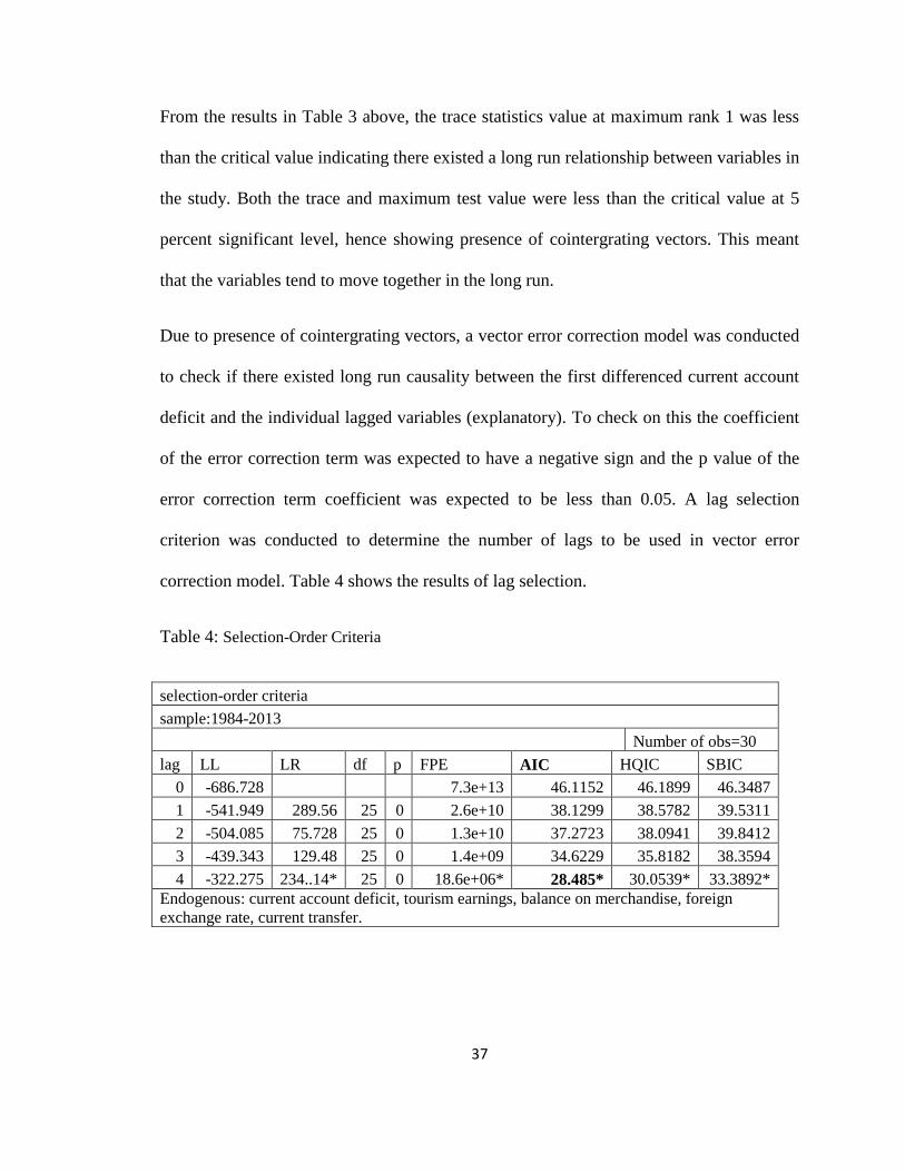
From the results in Table 3 above, the trace statistics value at maximum rank 1 was less
than the critical value indicating there existed a long run relationship between variables in
the study. Both the trace and maximum test value were less than the critical value at 5
percent significant level, hence showing presence of cointergrating vectors. This meant
that the variables tend to move together in the long run.
Due to presence of cointergrating vectors, a vector error correction model was conducted
to check if there existed long run causality between the first differenced current account
deficit and the individual lagged variables (explanatory). To check on this the coefficient
of the error correction term was expected to have a negative sign and the p value of the
error correction term coefficient was expected to be less than 0.05. A lag selection
criterion was conducted to determine the number of lags to be used in vector error
correction model. Table 4 shows the results of lag selection.
Table 4: Selection-Order Criteria
selection-order criteria
sample:1984-2013
Number of obs=30
lag LL LR df p FPE AIC HQIC SBIC
0 -686.728 7.3e+13 46.1152 46.1899 46.3487
1 -541.949 289.56 25 0 2.6e+10 38.1299 38.5782 39.5311
2 -504.085 75.728 25 0 1.3e+10 37.2723 38.0941 39.8412
3 -439.343 129.48 25 0 1.4e+09 34.6229 35.8182 38.3594
4 -322.275 234..14* 25 0 18.6e+06* 28.485* 30.0539* 33.3892*
Endogenous: current account deficit, tourism earnings, balance on merchandise, foreign
exchange rate, current transfer.

38
The study allowed for a maximum of up to four lags. The optimal number of lags for
each Vector error correction model was selected based on the lag selection criteria. The
study selected Akaike Information Criterion (AIC). From the table 4 the maximum lag
length selected for (AIC) was lag four. The study proceeded to conduct the vector error
correction model.
Table 5 Vector Error Correction Model (VECM)
Dependent Description Coef. Std.Err. Z p>[Z]
First differenced Current
account deficit _Cel L1 -0.2778 0.24093 -1.15 *0.049
First differenced Tourism earnings Lag one -4.44441 2.23918 -1.98 **0.047
Lag two 1.798818 2.943257 0.61 0.541
Lag three -6.14219 3.411888 -1.8 *0.072
First differenced Balance on merchandise
Lag one -0.23241 0.588722 -0.39 0.693
Lag two -1.24251 0.745562 -1.67 *0.096
Lag three 0.817996 0.743375 1.1 0.271
First differenced Foreign exchange rate
Lag one 0.637416 0.811811 0.79 0.432
Lag two 0.28549 0.861247 0.33 0.74
Lag three -0.46252 0.79394 -0.58 0.56
First differenced Current transfer Lag one -1.55756 1.137263 -1.37 0.171
Lag two -2.88497 1.420759 -2.03 *0.042
Lag three -1.21177 1.714851 0.71 0.48
Negative coefficient indicates presence of long run causality with prob < 0.05
** indicate significance at 0.05 and * indicates significance at 0.10
Table 5, shows that there is long run causality running from individual lagged variables
of tourism earnings, balance on merchandise, foreign exchange rate, current transfer to
current account deficit. This is because the coefficient of the error correction term is
negative (-0.277528) with a standard error of (0.2409286) and a z value of (-1.15). The

39
lagged variable indicated presence of short run causality. The study proceeded to conduct
granger causality test.
4.3 Granger Causality
This is a test conducted to check if one time series could be used to predict another time
series. Granger causality test can be used to forecast current account deficit in Kenya.
This can be done by checking presence of either bidirectional or unidirectional
relationships between the dependent variable and the independent variables. To check on
this, both t test and F test in lagged values were included. The results of granger test are
reported in Table 6.
Table 6 Granger Causality
Equation Excluded F df df_r Prob>F
Current account
Deficit
Tourism
Earnings 0.90997 4 9 0.0581
Tourism
Earnings
Current account
Deficit 5.8270 4 9 0.0135
Current account
Deficit
Balance on
merchandise 2.9488 4 9 0.0820
Balance on
merchandise
Current account
Deficit 0.93342 4 9 0.4866
Current account
Deficit
Foreign exchange
rate 0.95485 4 9 0.4765
Foreign exchange
rate
Current account
Deficit 0.6378 4 9 0.6486
Current account
Deficit
Current
Transfer 5.6368 4 9 0.0149
Current Transfer Current account
Deficit 2.9408 4 9 0.0825

40
The results from the analysis shows that after lagging the values four times, there was
statistical evidence of a unidirectional granger causality relationship running from
tourism earnings to current account deficit with a F test probability value of 0.0135 which
is below 5 percent significance level. While current transfer had a unidirectional granger
causality relationship running from current account deficit to current transfer with a F test
of 0.0149 which is below 5 percent significant level. After the granger causality test, the
study proceeded to run the regression line using the first differenced variables.
4.4 Regression Results
One of the key objective of the study was to determine the factor that affects the current
account in Kenya and establish the link between tourism earnings and current account
deficit in Kenya. Ordinary least square method was used to examine the linkage. The
estimation of the model is show in the table below.
Table 7 Regression Analyses
Variable Coef. Std.Err t P>[t]
Differenced Tourism earnings 0.33387 0.71428 0.47 0.644
Differenced balance on
Merchandise 0.557 0.05776 9.64 0.000
Differenced Foreign exchange rate -0.12619 0.39589 -0.32 0.752
Differenced Current transfer -0.33574 0.07443 -4.51 0.000
Constant -3.97427 2.6097 -1.52 0.139
Number of observations 33
Adjusted R-Squared 0.8775
Durbin Watson 2.05491

41
The results from the regression analysis indicated that adjusted R squared is 87.75
percent. This means that the explanatory variable explains approximately 88 percent of
the variation in current account deficit. It was also established that the value of Durbin
Watson at 2.054907 confirms that the coefficient are statistically different from zero. The
study also indicated that there was no serial correlation.
4.5 Discussion of the Estimation Results
The result obtained from the regression shows that the main independent variable
(tourism earnings) had a positive impact on current account deficit with a coefficient
0.333871. This coefficient was not statistically significant as revealed by its
corresponding standard error and p value of 0.644 which was above the significant value
of 0.05. This may partly be attributed to use of deflated data. While the positivity in the
coefficient of tourism earnings was in conformity to prior expected sign, it was also
observed that this contradicted findings from previous studies conducted by Ali Kemal
Celik, et al. (2013) ,Baharumshah, et al. (2003) and Greenidge, et al. (2011) who
established that tourism earnings has a significant relationship with current account
balance.
On the other hand, Balance on merchandise had a positive coefficient from the results of
the analysis. This was in conformity with the expected sign of positivity in relation to
current account deficit. Balance on merchandise was statistically significant to explain
variation in current account deficit with a probability value of less than 5 percent level. In
the results estimated, one percentage change in merchandise trade leads to approximately
0.5569 percent increase in current account deficit. This is to say that merchandise trade

42
balance has been the major cause of current account deficit. This results of balance on
merchandise was in conformity with Muwanga and Katamba (2005) who established in
their study that Uganda current account imbalances was due to high import export gap. It
must be noted that unlike tourism data, balance on merchandise statistics are properly
captured in Kenya, this could explain the robust regression outputs.
The results from the regression analysis also indicated that foreign exchange rate was in
conformity with the expected sign as its coefficient had a negative sign (-0.126). Foreign
exchange rate was not statistically significant to explain variation in the current account
deficit in Kenya since its probability value was above 5 percent significant level (0.752).
This contradicted previous studies conducted by other authors. According to Osoro
(2013) study of determinants of balance of payment, they established that real exchange
rate affects current account by causing a deficit when they decrease. They also found out
that real exchange rate had a significant relationship with current account balance in
Kenya though the impact was small.
The results from the analysis in the study showed that Current transfer had a negative
sign on its coefficient. Current transfer was also statistically significant to explain
variation in current account deficit in Kenya. This is in conformity with expectation, in
that one percent increase in current transfer will reduce current account deficit by 0.3357.
This is an indication that as more money come from net salary transfers and grants, then
current account moves from a deficit to a balance.

43
CHAPTER FIVE
5.0 CONCLUSION AND POLICY OPTIONS
This chapter presents the study conclusion and policy options. It also highlights the
limitation of the study and suggests areas for further research.
5.1 Conclusion
The aim of the study was to investigate the link between tourism earnings and current
account deficit and further determine factors that affect current account deficit in Kenya.
This was done by examining the behavior of each variable on current account deficit in
Kenya. From the findings it was established that the main independent variable (tourism
earnings) was not significant to explain variation in current account deficit. This was
expected since the study used proxy data.
Balance on merchandise and current transfer were found to be statistically significant to
explain variation in current account deficit and therefore the major contributor of the
current account deficit by the difference it creates in the account between exports and
imports of goods. The relationship it creates between current account deficits appeared to
be positive. This supports the ongoing trend on the persistent deficit which appear in the
current account in Kenya. Current transfer though statistically significant, is the smallest
component in current account explaining the change in current account imbalances.

44
5.2 Policy Options
The findings of this study indicates that balance on merchandise is the key factors that
affects current account in Kenya. This is the net balance between import of goods and
export of goods. Currently the balance on merchandise has been in a deficit and the
import export gap has expanded tremendously. This gap has been attributed to higher
consumption of imported goods and lower exports of raw agricultural products. To
improve on balance on merchandise, the government should control the amount of
imports that comes into the country through the use of expenditure switching policies.
This are policies which the government may use to switch consumers (local citizens)
away from imports and towards home produced goods. The government can do this by
using imports control such as tariffs and devaluating the exchange rate. The government
needs to offer more abroad than it has done so far by besides everything else, enhancing
the competiveness of her exports so as to augment her shares in the world market.
Policies ought to be prioritized on value addition activities in Kenya’s export sector since
this can improve the total volume of Kenyan export thus reduction of the gap between
imports and exports .
The governments ought to bear on empowering and creating the tourism industry. This
can be done by ensuring that there is proper infrastructure in place. Recent advances in
airline transportation can play a real part in breaking down transportation obstructions.
Kenya being an extensive nation ought to recognize the significance of tourism, and
raising the level of public awareness is likely to prompt further revenue generations in the
future. Kenya for the most part should focus on conference tourism as this is an area
which has not been exploited yet.

45
Enhancing vision 2030 strategies is key since tourism has been encompassed in the blue
print as one of the key pillar that can boost growth in the economy. Though the findings
suggest that tourism was not statistically significant to explain change in current account
deficit, tourism is important since it is the second largest contributor of foreign exchange
earnings and if properly marketed may boost economic growth in the economy. More
over focus need to be placed on the improvement of security within the country, and
development of infrastructure.
5.3 Area for future research
It was clear from the study conducted that data on tourism earnings was not properly
captured hence the use of proxy data. There is a need to research on a robust tourism data
capture mechanism that will reflect the true position of tourism earnings in Kenya. There
is also a need for proper research to be undertaken on the analysis of determinant of
tourism sector growth in Kenya.

46
6.0 REFERENCES
Alexander, S. S. (1952). Effects of a Devaluation on a Trade Balance. IMF Staff Papers,
2(2), 263-278.
Ahearn, J. (2002). Should South East Asia Devalue? Issues in political economy, 11.
Alemayehu, G., Ndung'u, N., & Zerfu, D. (2012). Applied time series econometrics.
Brida, J. G., Carrera, E. S., & Risso, W. A. (2008). Tourism’s impact on long-run
Mexican economic growth. Economics Bulletin, 3(21), 1-8.
Baharumshah, A. Z., Lau, E., & Fountas, S. (2003). On the sustainability of current
account deficits: evidence from four ASEAN countries. Journal of Asian Economics,
14(3), 465-487.
Bodman, P. M. (1997). The Australian trade balance and current account: a time series
perspective. International Economic Journal, 11(2), 39-57.
Çelik, A. K., Özcan, S., Topcuoğlu, A., & Yildirim, K. E. (2013). Effects of the tourism
industry on the balance of payments deficit. Anatolia, 24(1), 86-90.
Fisher, S. (1988) Real balance, the exchange Rate, and Indexation, Real Variable in
Disinflation. Quarterly Journal of economics, 103(1)
Greenidge, K., Holder, C., & Moore, A. (2011). Current account deficit sustainability: the
case of Barbados. Applied Economics, 43(8), 973-984.
International Monetary Fund (1977). The Monetary Approach to Balance of Payments.
Washington, DC, International Monetary Fund.
Johansen, S. (1988). Statistical analysis of cointegration vectors. Journal of economic
dynamics and control, 12(2), 231-254.
Johnson, H. G. (1972). The monetary approach to balance-of-payments theory. Journal of
financial and quantitative analysis, 7(02), 1555-1572.
Kenya National Bureau of Statistics, & Kenya. Central Bureau of Statistics. (Various).
Statistical abstract. Kenya National Bureau of Statistics.
Metzler, L. (1948). A Survey of Contemporary Economics, Vol. I, Richard D. Irwin.
INC, Homewood, IL.
Muwanga-Zake, E. S. K., & Katamba, M. P. (2005). Capital Flows and Current Account
Sustainability–Uganda’s Experience: 1994-2004’. In Workshop on “Capital flows and
current account sustainability in African economies”, organized by Economic and Social
Policy Division, United Nations Economic Commission for Africa (pp. 21-22).

47
Matsubayashi, Y. (2005). Are US current account deficits unsustainable?: Testing for the
private and government intertemporal budget constraints. Japan and the World Economy,
17(2), 223-237.
Ongan, S. (2008). The sustainability of current account deficits and tourism receipts in
Turkey. The International Trade Journal, 22(1), 39-62.
Osoro, K. (2013). Determinants of Balance Of Payments in Kenya. European Scientific
Journal, 9(16).
Outlook, A. E. (2012). Kenya 2012. African Economic Outlook 2012.
Ogus Binatli, A., & Sohrabji, N. (2008). Intertemporal solvency of Turkey’s current
account (No. 0805). Izmir University of Economics.
Ranciere, R., Throckmorton, N. A., Kumhof, M., Lebarz, C., & Richter, A. W. (2012).
Income Inequality and Current Account Imbalances (No. 12/8). International Monetary
Fund.
Schubert, S. F., & Brida, J. G. (2009). Macroeconomic effects of changes in tourism
demand: a simple dynamic model. Tourism Economics, 15(3), 591-613.
Sinclair, T. & Stabler, M. (2002). The Economics of The impact of tourism on economic
growth and Tourism. Routledge, London. Development in Africa. Middle Tennessee
State
World Bank (2012), Walking the Tightrope: Rebalancing Kenya Economy. Nairobi;
World Bank, June 2012
World Tourism Organization (WTO, 1990, Travel and tourism barometer). Madrid:
WTO
World Tourism Organization (WTO, 1994, Travel and tourism barometer). Madrid:
WTO
World Tourism Organization (UNWTO, 2000, Tourism Highlight Editions): WTO.
World Tourism Organization (UNWTO, 2005, Tourism Highlight Editions): WTO.
World Tourism Organization (UNWTO, 2007, Tourism Highlight Editions): WTO.
World Tourism Organization (UNWTO, 2008, Tourism Highlight Editions): WTO.
World Tourism Organization (UNWTO, 2010, Tourism Highlight Editions): WTO.
World Tourism Organization (UNWTO, 2013, Tourism Highlight Editions): WTO.

48
Yol, M. A. (2009). Testing the sustainability of current account deficits in developing
economies: Evidence from Egypt, Morocco, and Tunisia. The Journal of Developing
Areas, 43(1), 177-197.

49
APPENDICIES
APPENDIX 1 UNIT ROOT TEST AT LEVEL
LEVEL
Number of
Obs=33
Variable Test Statistics
1% Critical
Value
5% Critical
value
10% Critical
value P-Value
Current
account Deficit 1.199 -4.306 -3.568 -3.221 1.0000
Tourism
Earnings -1.114 -4.306 -3.568 -3.221 0.9267
Balance on
merchandise 1.529 -4.306 -3.568 -3.221 1.0000
Foreign
exchange rate -1.608 -4.306 -3.568 -3.221 0.7895
Current transfer -2.173 -4.306 -3.568 -3.221 0.5049
Income per-
capita -5.630 -4.306 -3.568 -3.221 0.0000
APPENDIX 2 UNIT ROOT TEST AT FIRST DIFFERENCE
FIRST DIFFERENCE
Number of
Obs=32
Variable Test Statistics
1% Critical
Value
5% Critical
value
10% Critical
value P-Value
Current
account Deficit -5.260 -4.316 -3.572 -3.223 0.0001
Tourism
Earnings -6.143 -4.316 -3.572 -3.223 0.0000
Balance on
merchandise -4.077 -4.316 -3.572 -3.223 0.0068
Foreign
exchange rate -5.298 -4.316 -3.572 -3.223 0.0001
Current transfer -14.03 -4.316 -3.572 -3.223 0.0000

50
APPENDIX 3 COINTERGRATION TEST
Current account Deficit, Tourism Earnings ,Balance on merchandise ,Foreign
exchange rate, Current transfer, trend(constant) max
Johansen tests for cointergration
Trend: constant Number of obs=32
sample:1982-2013 Lags=2
maximum rank parms LL eigenvalue trace statistics 5% critical
value
0 30 -580.21819 . 93.0266 68.52
1 39 -554.08503 0.80472 40.7602* 47.21
2 46 -544.39425 0.45429 21.3787 29.68
3 51 -538.27168 0.31796 9.1335 15.41
4 54 -534.71924 0.19911 2.0287 3.76
5 55 -533.70491 0.06143
maximum rank parms LL eigenvalue max statistics 5% critical
value
0 30 -580.21819 . 52.2663 33.46
1 39 -554.08503 0.80472 19.3816 27.07
2 46 -544.39425 0.45429 12.2451 20.97
3 51 -538.27168 0.31796 7.1049 14.07
4 54 -534.71924 0.19911 2.0287 3.76
5 55 -533.70491 0.06143
APPENDIX 4 SELECTION ORDER CRITERIA
Current account Deficit Tourism Earnings Balance on merchandise Foreign exchange rate Current transfer
selection-order criteria
sample:1984-2013
Number of obs=30
lag LL LR df p FPE AIC HQIC SBIC
0 -686.728 7.3e+13 46.1152 46.1899 46.3487
1 -541.949 289.56 25 0 2.6e+10 38.1299 38.5782 39.5311
2 -504.085 75.728 25 0 1.3e+10 37.2723 38.0941 39.8412
3 -439.343 129.48 25 0 1.4e+09 34.6229 35.8182 38.3594
4 -322.275 234..14* 25 0 18.6e+06* 28.485* 30.0539* 33.3892*
Endogenous: Current account Deficit Tourism Earnings Balance on merchandise Foreign exchange rate Current transfer
Exogenous: _cons

51
APPENDIX 5 VECTOR ERROR CORRECTION MODEL
Current account Deficit Tourism Earnings Balance on merchandise
Foreign exchange rate Current transfer , trend ( constant) lags (4)
vector error - correction model NO. of obs=30
sample:1984-2013 AIC=33.1885
log likelihood=-408.8275 HQIC=34.51833
Det(sigma_m1)= 472495.8 SBIC=37.34539
Equation parms RMSE R-sq chi2 p>chi2
First differenced Current account deficit 17 18.1643 0.9010 118.3714 0.0000
First differenced Tourism earnings 17 3.35691 0.8452 70.97676 0.0000
First differenced Balance on merchandise 17 31.2902 0.8866 101.6444 0.0000
First differenced Foreign exchange rate 17 6.95734 0.4678 11.42908 0.8334
First differenced Current transfer 17 12.2927 0.9465 203.1949 0.0000
coef std.Err. z p>z 95% conf . Interval
First differenced Current account deficit
Cointergrating
equation 1 -0.2777528 0.240986 -1.15 0.049 -.1944585 0.7499641
Current account deficit
Lag one -1.155947 0.796712 -1.45 0.147 -2.71747 0.405580
Lag two -0.117503 0.639299 -0.18 0.854 -1.370507 1.135501
Lag three 0.0088057 0.4953525 0.02 0.986 -.9620674 0.9796787
Tourism earnings
Lag one -4.444412 2.239218 -1.98 0.047 -8.833198 -.0556264
Lag two 1.798818 2.943257 0.61 0.541 -3.969861 7.567496
Lag three -6.142164 3.411888 -1.80 0.072 -12.82937 0.5449833
Balance on
Merchandise
Lag one -.2324139 .5887221 -.39 .0693 -1.386288 .9214603

52
Lag two -1.242505 0745562 -1.67 0.096 -2.70378 .2187697
Lag three .8179963 .743375 1.10 0.271 -.6389919 2.274984
Foreign exchange
rate
Lag one .6374164 .8118107 0.79 0.432 -.9537033 2.228536
Lag two .2854902 .8612466 0.33 0.740 -1.402522 1.973503
Lag three -.4625175 .7939401 -0.58 0.560 -2.018612 1.093576
Current Transfer
Lag one -1.55756 1.137263 -1.37 0.171 -3.786555 .6714356
Lag two -2.884971 1.420759 -2.03 0.042 -5.669607 -.1003349
Lag three 1.211769 1.714851 0.71 0.480 -2.149277 4.572816
Constant 5.428013 8.367028 0.65 0.517 -10.97106 21.82709
APPENDIX 6 JOHNSEN NORMALIZATION RESTRICTION IMPOSE
Equation parms chi2 p>chi2
Cointergrating
equation 4 689.8285 0.0000
identification: beta is exactly identified
Johnsen normalization restriction impose
beta coef. std.Err. z p>z 95% conf. Interval
Cointergrating
equation
Current
account deficit 1
Tourism
earnings 5.26521 .3914146 13.45 0.0000 4.498051 6.032368
Balance on
merchandise 1.885318 .3707915 5.08 0.0000 1.15858 2.612056
Foreign
exchange rate -1.305232 .2723488 -4.79 0.0000 -1.839026 -.7714384
Current
transfer 2.674492 .8710112 3.07 0.002 .9673415 4.381643
constant 27.7245

53
APPENDIX 7 GRANGER CAUSALITY TEST
Equation Excluded F df df_r Prob>F
Current
account
Deficit
Tourism
Earnings 0.90997 4 9 0.0581
Tourism
Earnings
Current
account
Deficit 5.6368 4 9 0.0149
Current
account
Deficit
Balance on
merchandise 2.9488 4 9 0.082
Balance on
merchandise
Current
account
Deficit
0.93342 4 9 0.4866
Current
account
Deficit
Foreign
exchange rate 0.95485 4 9 0.4765
Foreign
exchange rate
Current
account
Deficit
0.6378 4 9 0.6486
Current
account
Deficit
Current
Transfer 5.6368 4 9 0.0149
Current
Transfer
Current
account
Deficit
2.9408 4 9 0.0825

54
APPENDIX 8 REGRESSION ANALYSIS
Number of obs=33
regress current account deficit, tourism earnings, balance on
merchandise, foreign exchange rate and current transfer F(4, 28)= 58.30
source ss df ms prob>F=0.0000
Model 34252.18 4 8563.045 R-squared=0.8928
Residual 4112.883 28 146.8887 Adj R-
squared=0.8775
Total 38365.06 32 1198.908 Root MSE=12.12
First differenced Current account deficit
coef. std.Err. t p>t 95% conf. Interval
First differenced Tourism earnings
0.333871 0.714279 0.47 0.644 -1.12926 1.797005
First differenced Balance on merchandise
0.556998 0.057765 9.64 0.000 0.438672 0.675324
First differenced Foreign exchange rate
-0.12619 0.395889 -0.32 0.752 -0.68475 9371349
First differenced Current transfer
-0.33574 0.074431 -4.51 0.000 -0.4882 -0.18327
constant -3.97427 2.6097 -1.52 0.139 -9.32 1.371456
Durbin-Watson d-statistics (5, 33) = 2.054907
APPENDIX 9 SERIAL CORRELATION TEST
estat bdodfrey
Breusch-Godfrey LM test for auto correlation
lag(p) chi2 df prob>chi2
1 0.040 1 0.8421
H0: no serial correlation