Toward a more rigorous goodness-of-fit test for evaluating simultaneous

radio and γ-ray pulsar light curve fits

A.S. Seyffert, C. Venter, A.K. Harding

Introduction

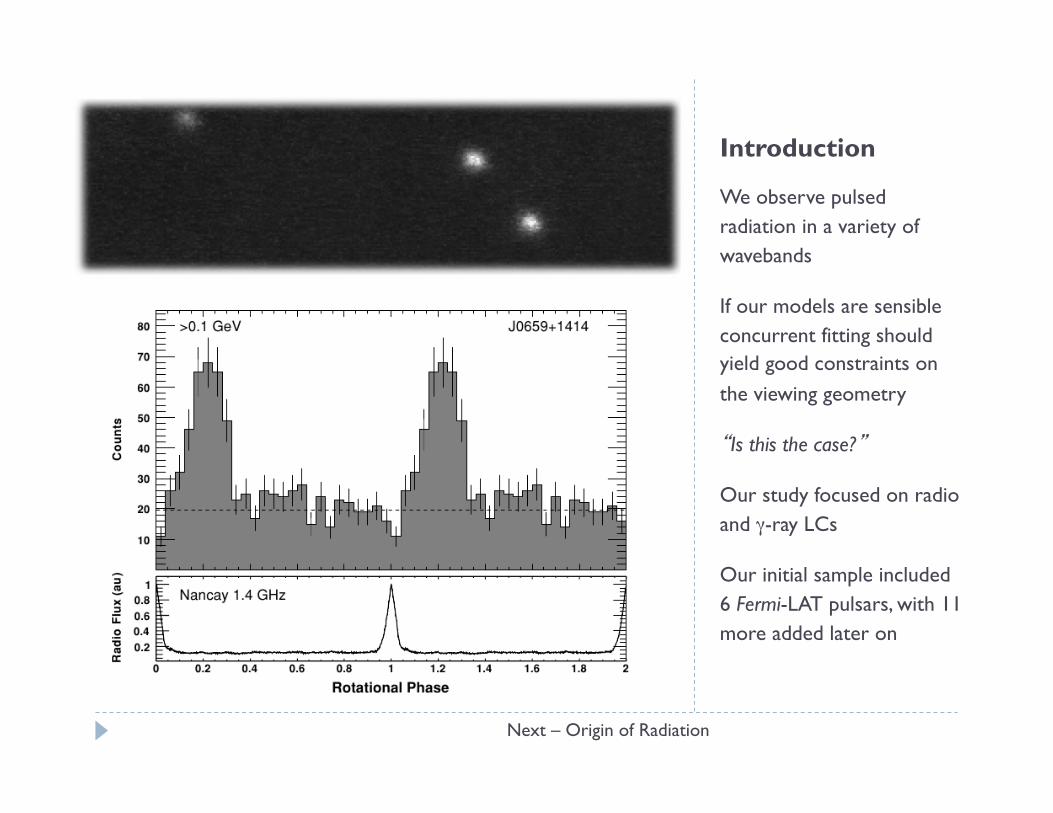
We observe pulsed radiation in a variety of wavebands

If our models are sensible concurrent fitting should yield good constraints on the viewing geometry

“Is this the case?”

Our study focused on radio and γ-ray LCs

Our initial sample included 6 Fermi-LAT pulsars, with 11 more added later on

Next – Origin of Radiation

Introduction

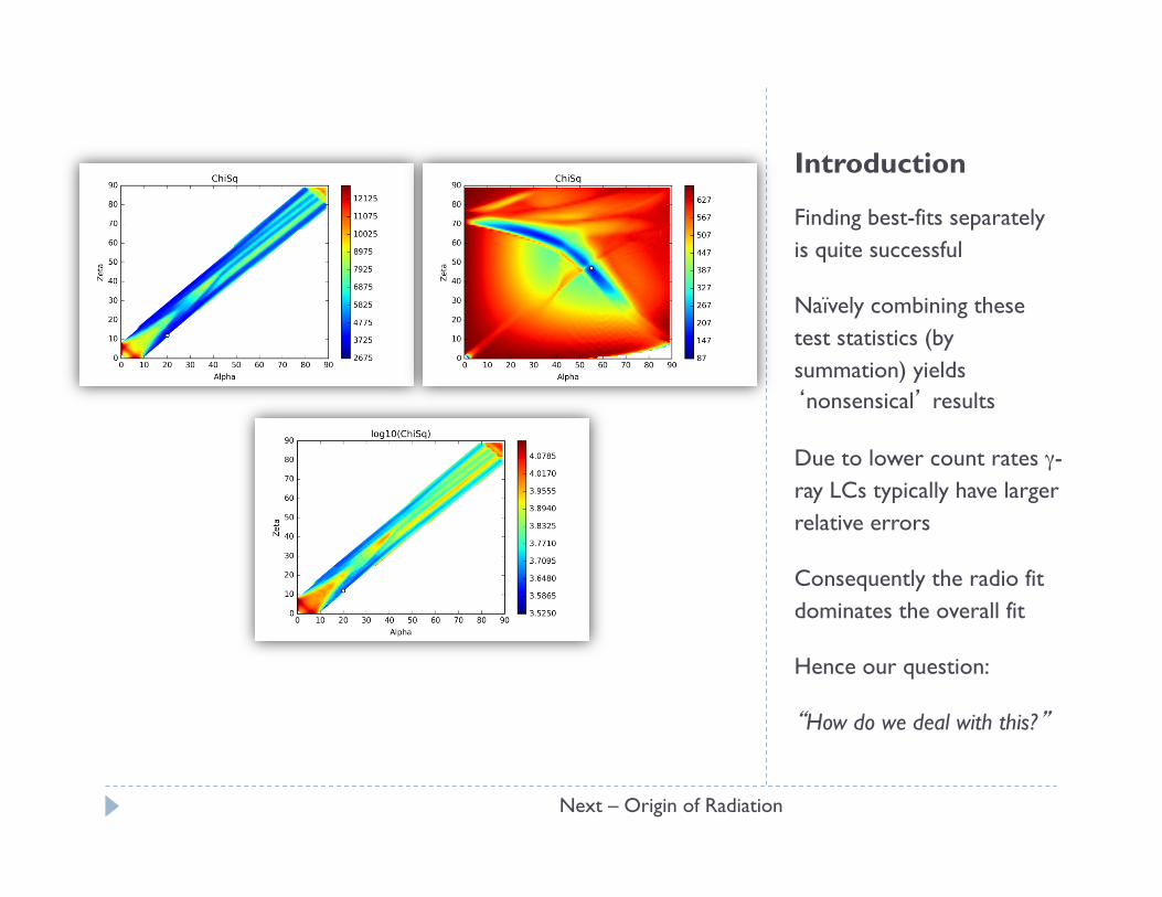
Finding best-fits separately is quite successful

Naïvely combining these test statistics (by summation) yields ‘nonsensical’ results

Due to lower count rates γ-ray LCs typically have larger relative errors

Consequently the radio fit dominates the overall fit

Hence our question:

“How do we deal with this?”

Next – Origin of Radiation

Background

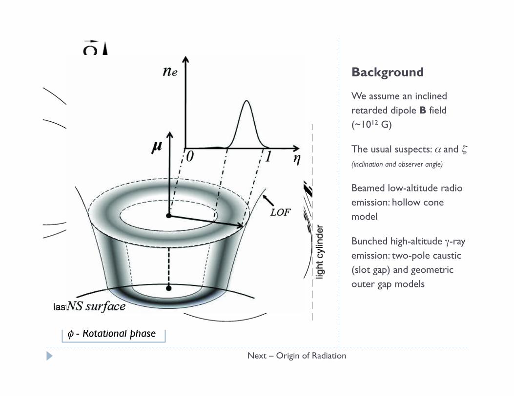
We assume an inclined retarded dipole B field (~1012 G)

The usual suspects: α and ζ (inclination and observer angle)

Beamed low-altitude radio emission: hollow cone model

Bunched high-altitude γ-ray emission: two-pole caustic (slot gap) and geometric outer gap models

Next – Origin of Radiation

α - Inclination angle ζ - Observer angle φ - Rotational phase

Extracting LCs

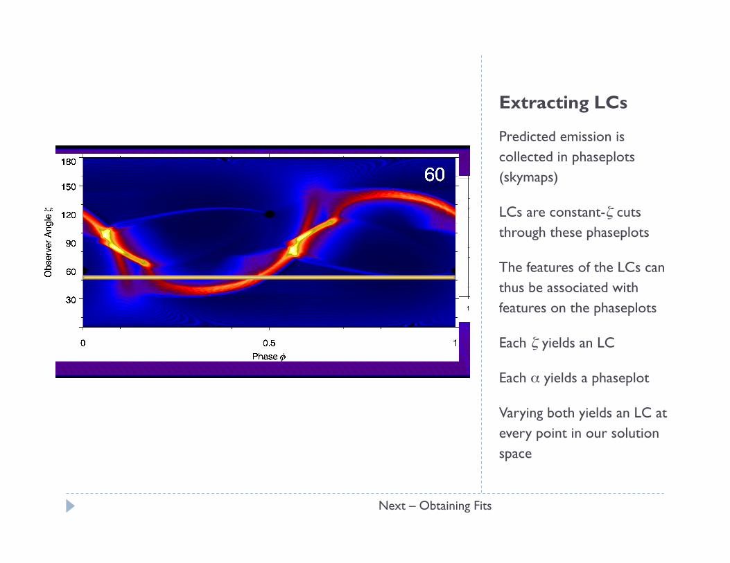
Predicted emission is collected in phaseplots (skymaps)

LCs are constant-ζ cuts through these phaseplots

The features of the LCs can thus be associated with features on the phaseplots

Each ζ yields an LC

Each α yields a phaseplot

Varying both yields an LC at every point in our solution space

Next – Obtaining Fits

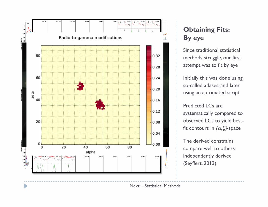
Obtaining Fits: By eye

Since traditional statistical methods struggle, our first attempt was to fit by eye

Initially this was done using so-called atlases, and later using an automated script

Predicted LCs are systematically compared to observed LCs to yield best-fit contours in (α,ζ)-space

The derived constrains compare well to others independently derived (Seyffert, 2013)

Next – Statistical Methods

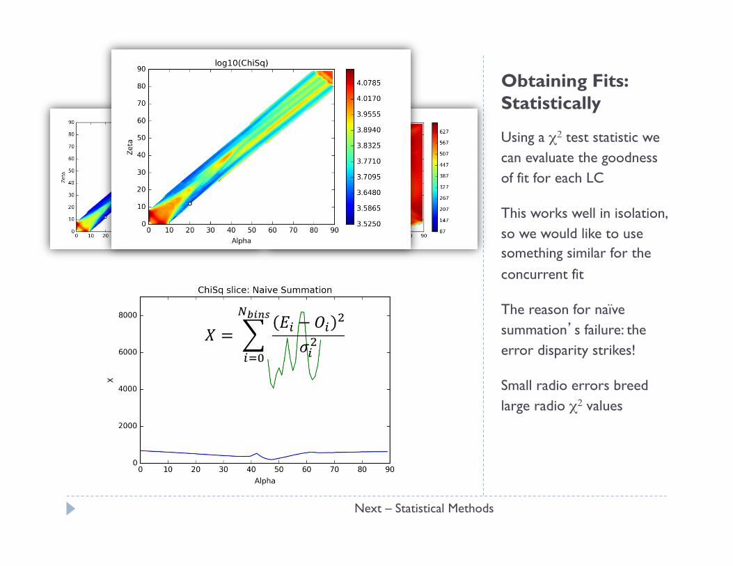
Obtaining Fits: Statistically

Using a χ2 test statistic we can evaluate the goodness of fit for each LC

This works well in isolation, so we would like to use something similar for the concurrent fit

The reason for naïve summation’s failure: the error disparity strikes!

Small radio errors breed large radio χ2 values

Next – Statistical Methods

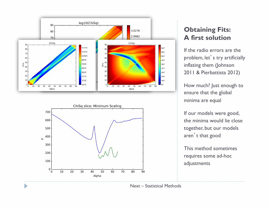
Obtaining Fits: A first solution

If the radio errors are the problem, let’s try artificially inflating them (Johnson 2011 & Pierbattista 2012)

How much? Just enough to ensure that the global minima are equal

If our models were good, the minima would lie close together, but our models aren’t that good

This method sometimes requires some ad-hoc adjustments

Next – Statistical Methods

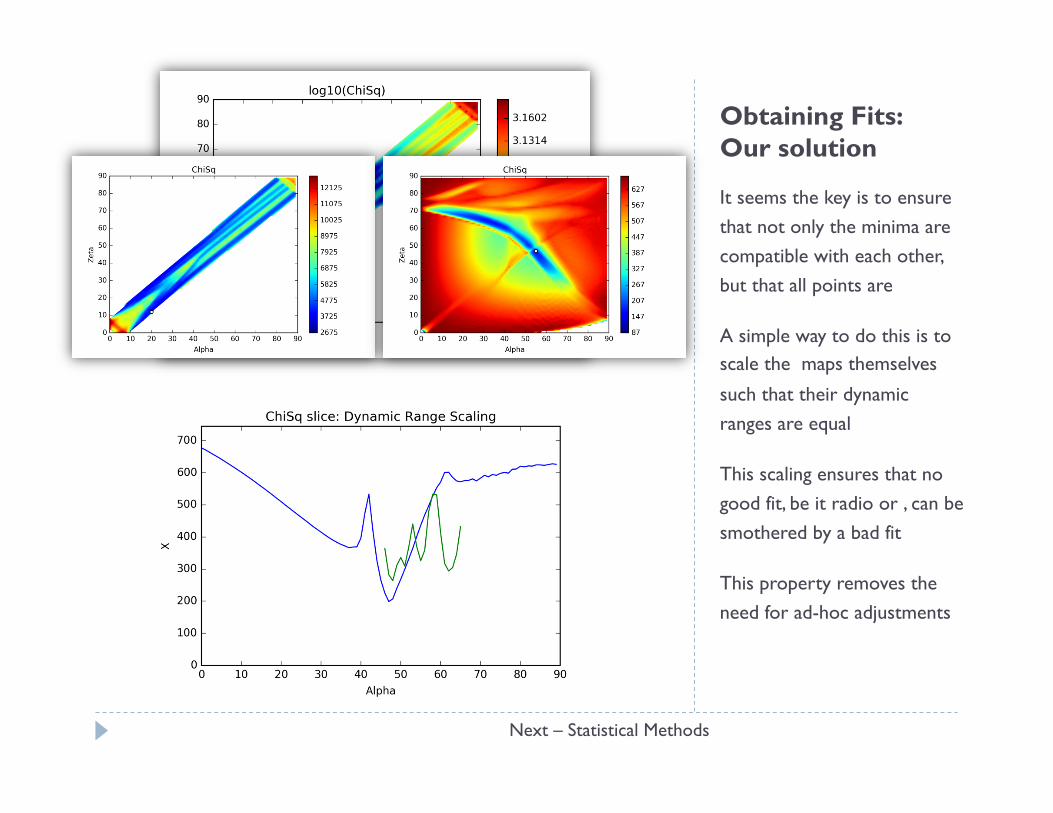
Obtaining Fits: Our solution

It seems the key is to ensure that not only the minima are compatible with each other, but that all points are

A simple way to do this is to scale the maps themselves

such that their dynamic ranges are equal

This scaling ensures that no good fit, be it radio or , can be smothered by a bad fit

This property removes the need for ad-hoc adjustments

Next – Statistical Methods

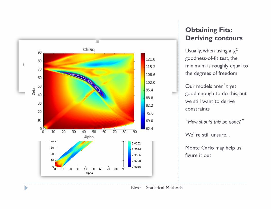
Obtaining Fits: Deriving contours

Usually, when using a χ2 goodness-of-fit test, the minimum is roughly equal to the degrees of freedom

Our models aren’t yet good enough to do this, but we still want to derive constraints

“How should this be done?”

We’re still unsure...

Monte Carlo may help us figure it out

Next – Statistical Methods

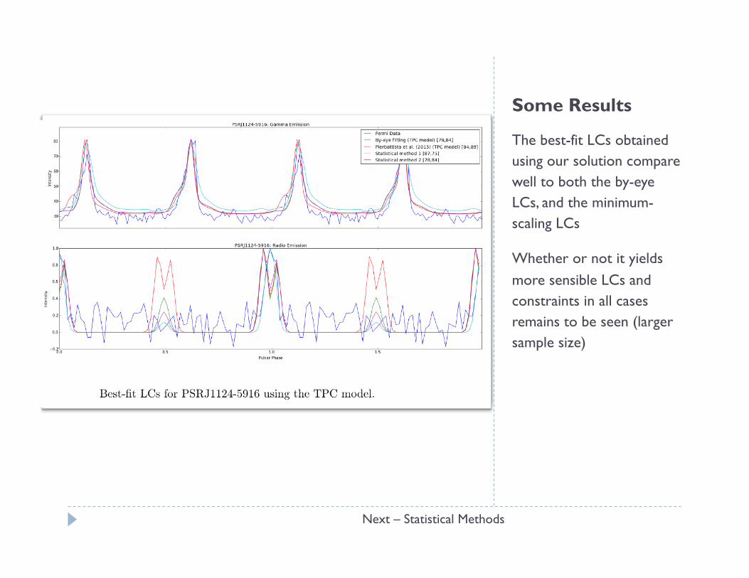
Some Results

The best-fit LCs obtained using our solution compare well to both the by-eye LCs, and the minimum-scaling LCs

Whether or not it yields more sensible LCs and constraints in all cases remains to be seen (larger sample size)

Next – Statistical Methods

Conclusion }  This new approach to determining the goodness-of-fit of

concurrent fits seems to achieve its goal without any subjective adjustments needed

}  It also promises to be extensible: X-ray LCs? }  The contours are still an unresolved issue }  There are also some assumptions involved that need to

be checked since any derived contours will be sensitive to these assumptions

Future Work }  Derive a sensible way to draw contours }  Apply this technique to a large number and large variety

of pulsars to check whether it really doesn’t need ad-hoc adjustments

}  Other test statistics? }  Other magnetic fields? }  Current sheet?? }  Incorporating the X-ray LCs and models in preparation

for NICER }  Use concurrent fitting results to refine the models used

Thank you…

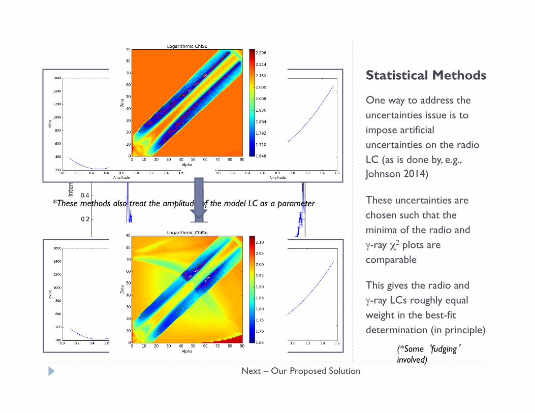
Statistical Methods

One way to address the uncertainties issue is to impose artificial uncertainties on the radio LC (as is done by, e.g., Johnson 2014)

These uncertainties are chosen such that the minima of the radio and γ-ray χ2 plots are comparable

This gives the radio and γ-ray LCs roughly equal weight in the best-fit determination (in principle)

γ radio

*These methods also treat the amplitude of the model LC as a parameter

(*Some ‘fudging’ involved)

Next – Our Proposed Solution

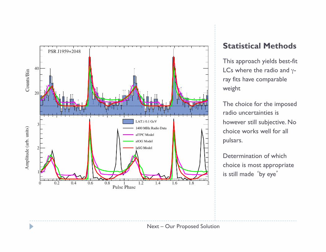
Statistical Methods

This approach yields best-fit LCs where the radio and γ-ray fits have comparable weight

The choice for the imposed radio uncertainties is however still subjective. No choice works well for all pulsars.

Determination of which choice is most appropriate is still made ‘by eye’

Next – Our Proposed Solution

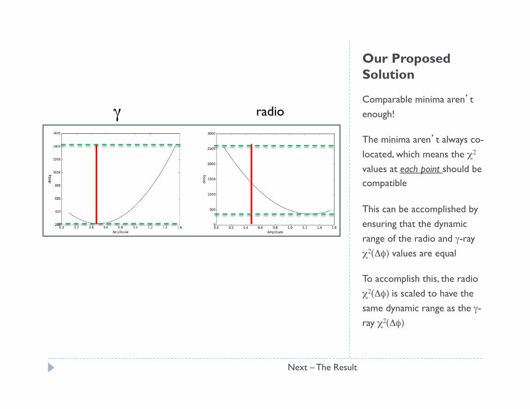
Our Proposed Solution

Comparable minima aren’t enough!

The minima aren’t always co-located, which means the χ2 values at each point should be compatible

This can be accomplished by ensuring that the dynamic range of the radio and γ-ray χ2(Δφ) values are equal

To accomplish this, the radio χ2(Δφ) is scaled to have the same dynamic range as the γ-ray χ2(Δφ)

γ radio

Next – The Result

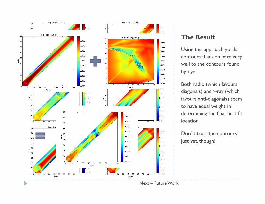
The Result

Using this approach yields contours that compare very well to the contours found by-eye

Both radio (which favours diagonals) and γ-ray (which favours anti-diagonals) seem to have equal weight in determining the final best-fit location

Don’t trust the contours just yet, though!

Next – Future Work

Future Work }  Sensible Errors?

}  The manipulation of the radio χ2 values means that usual confidence intervals don’t carry the same meaning after combination

}  Essentially the combined metric is Γ-distributed, making confidence determination more difficult

}  Applying this to actual pulsars }  The results of our previous study (Seyffert, 2013) will be re-

evaluated using this new approach. This will serve as a sort of cross-calibration

}  This approach will also be used to evaluate how well different magnetospheric models fare in reproducing the observed LCs