April 2015

NASA/TM–2015-218706

Toward a Nonlinear Acoustic Analogy: Turbulence as a Source of Sound and Nonlinear Propagation Steven A. E. Miller Langley Research Center, Hampton, Virginia

NASA STI Program . . . in Profile

Since its founding, NASA has been dedicated to the advancement of aeronautics and space science. The NASA scientific and technical information (STI) program plays a key part in helping NASA maintain this important role.

The NASA STI program operates under the auspices of the Agency Chief Information Officer. It collects, organizes, provides for archiving, and disseminates NASA’s STI. The NASA STI program provides access to the NTRS Registered and its public interface, the NASA Technical Reports Server, thus providing one of the largest collections of aeronautical and space science STI in the world. Results are published in both non-NASA channels and by NASA in the NASA STI Report Series, which includes the following report types:

• TECHNICAL PUBLICATION. Reports of

completed research or a major significant phase of research that present the results of NASA Programs and include extensive data or theoretical analysis. Includes compilations of significant scientific and technical data and information deemed to be of continuing reference value. NASA counter-part of peer-reviewed formal professional papers but has less stringent limitations on manuscript length and extent of graphic presentations.

• TECHNICAL MEMORANDUM. Scientific and technical findings that are preliminary or of specialized interest, e.g., quick release reports, working papers, and bibliographies that contain minimal annotation. Does not contain extensive analysis.

• CONTRACTOR REPORT. Scientific and technical findings by NASA-sponsored contractors and grantees.

• CONFERENCE PUBLICATION. Collected papers from scientific and technical conferences, symposia, seminars, or other meetings sponsored or co-sponsored by NASA.

• SPECIAL PUBLICATION. Scientific, technical, or historical information from NASA programs, projects, and missions, often concerned with subjects having substantial public interest.

• TECHNICAL TRANSLATION. English-language translations of foreign scientific and technical material pertinent to NASA’s mission.

Specialized services also include organizing and publishing research results, distributing specialized research announcements and feeds, providing information desk and personal search support, and enabling data exchange services.

For more information about the NASA STI program, see the following:

• Access the NASA STI program home page at

http://www.sti.nasa.gov

• E-mail your question to help@sti.nasa.gov

• Phone the NASA STI Information Desk at 757-864-9658

• Write to: NASA STI Information Desk Mail Stop 148 NASA Langley Research Center Hampton, VA 23681-2199

National Aeronautics and Space Administration Langley Research Center Hampton, Virginia 23681-2199

April 2015

NASA/TM–2015-218706

Toward a Nonlinear Acoustic Analogy: Turbulence as Source of Sound and Nonlinear Propagation Steven A. E. Miller Langley Research Center, Hampton, Virginia

Available from:

NASA STI Program / Mail Stop 148 NASA Langley Research Center

Hampton, VA 23681-2199 Fax: 757-864-6500

Acknowledgments

The author is grateful for continuous support from the National Aeronautics and Space Administration (NASA), Advanced Air Vehicles Program, Commercial Supersonic Technology Project. Brian Howerton of NASA Langley Research Center provided measurements from the NASA Langley Liner Lab Normal Incidence Tube. Emily Mazur, a 2012 NASA Langley Aerospace Research Student Scholars Program participant, is acknowledged for evaluating numerically the Blackstock bridging function.

The use of trademarks or names of manufacturers in this report is for accurate reporting and does not constitute an official endorsement, either expressed or implied, of such products or manufacturers by the National Aeronautics and Space Administration.

Abstract

An acoustic analogy is proposed that directly includes nonlinear prop-agation effects. We examine the Lighthill acoustic analogy and replacethe Green’s function of the wave equation with numerical solutions of thegeneralized Burgers’ equation. This is justified mathematically by usingsimilar arguments that are the basis of the solution of the Lighthill acous-tic analogy. This approach is superior to alternatives because propaga-tion is accounted for directly from the source to the far-field observer in-stead of from an arbitrary intermediate point. Validation of a numericalsolver for the generalized Burgers’ equation is performed by comparingsolutions with the Blackstock bridging function and measurement data.Most importantly, the mathematical relationship between the Navier-Stokes equations, the acoustic analogy that describes the source, andcanonical nonlinear propagation equations is shown. Example predic-tions are presented for nonlinear propagation of jet mixing noise at thesideline angle.

1

Nomenclature

SymbolsA Arbitrary vector quantityAijlm Coefficient matrixAij Subset of Aijlm

Bn Fourier coefficients of BBFc Speed of soundD Nozzle exit diameterDj Fully expanded diametereo Total energyF Fourier series dependent on xg Arbitrary function or Green’s functionJn Bessel function of the first kind of order nj Integer indexK Fourier coefficientk Wavenumberkmax Maximum turbulent kinetic energy

within jet plumel Turbulent length scaleM Mach numberMa Acoustic Mach numberMc Convective Mach number constantMd Design Mach numberMj Fully expanded Mach numberm Integer indexPf Scaling constant for spectral densityPr Prandtl numberp Pressureq Heat-fluxq̃ Square of p̃R Gas constant or propagation distanceRijlm Two-point cross-correlation of Lighthill

stress tensorr Vector from source to observerr Radial coordinateS Spectral densitySt Strouhal numberSy Equivalent source strength per unit lengthT Thermodynamic temperature

Td Thermal diffusion rateTij Lighthill stress tensort Timeu Velocityx Observer or positiony Source position or particle displacementyc Jet potential core lengthα Atmospheric absorption coefficientβ Coefficient of nonlinearity

or dispersion coefficientβs A constant within the two-point

cross-correlationΓ Group of coefficients involving nonlinearityγ Ratio of specific heatsδ Dirac delta function or viscous termsδij Kronecker delta functionε β(ρ∞c

3∞)−1

η(ξ, η, ζ) Source separation vectorµ Kinematic viscosityν Dynamic viscosityξ Momentum in Lagrangian coordinates or

source separation in x directionρ Densityσ Shock formation distance

or amplification factorτ Retarded timeτs Turbulent time scaleτij Viscous stress tensorΦsh Earnshaw phase angleφ Arbitrary vector quantity or wave

emission timeω Radial frequency

AbbreviationsBBF Blackstock bridging functionNIT Normal Incidence TubePSD Power spectral densitySPL Sound pressure levelTTR Total temperature ratio

2

1 Introduction

The physical mechanism and associated mathematical model to predict acoustic radiation fromhigh speed compressible fluid turbulence continues to elude investigators after decades of research.In most fluid flows, the intensity of turbulence gives rise to acoustic radiation that propagatesaccording to the theory of linear acoustics and dissipative effects dominate nonlinear effects. Whenturbulence is highly intense the resultant acoustic waves have magnitudes that result in nonlinearpropagation due to dominance of nonlinear terms over dissipative terms contained in the equationsof motion. The radiating waves contain all non-zero frequency components, are very energetic, andcoalesce into many discontinuities (shock waves). Here, we seek a unified theory of the radiationsource using an acoustic analogy combined with the nonlinear propagation effects approximatelygoverned by the generalized Burgers’ equation.

High intensity compressible turbulence is present within the exhaust flow created by rocket andhigh performance air breathing jet engines. The acoustic radiation created by these exhaust flowsis potentially harmful to the flight vehicle airframe, launchpad, or flight deck through the mecha-nism of sonic fatigue or sonic failure. It is also potentially harmful or annoying to the surroundingcommunity and natural environment. A few recent investigations (among many conducted overdecades) illustrate the relevance of this contemporary problem via the noise produced by aircraft.Recently, Neilsen et al. [1] conducted measurements of the ‘F-22A Raptor’ flight vehicle with after-burning engines. They examined the spectral characteristics spatially and the waveforms’ nonlinearindicators as described by Gee et al. [2], and showed that nonlinear propagation effects are impor-tant. Though many nonlinear indicators have been proposed, Gee et al. [2] created two that arecomplimentary to traditional spectral measurement approaches, and successfully separated geomet-ric acoustic effects from nonlinear propagation effects. Petitjean et al. [3] performed experiments toexamine nonlinear distortion of acoustic waves and waveforms in the time and frequency domains.They proposed that the convective Mach number of turbulent structures is highly correlated withnonlinear effects, which is certainly the case for high speed rocket and jet exhaust. Highly energeticjet noise spectra were recently analyzed by Tam and Parrish [4], and they proposed that the di-vergence of measurements from relatively low intensity similarity spectra might be due to indirectcombustion noise from the afterburner. The peak intensities calculated by Tam and Parrish [4]are 178 dB. Morfey and Howell [5] conducted flight tests and showed that the inclusion of finite-amplitude noise propagation theory must be used to account for observed aircraft flyover effects.Thus, prediction approaches for jet noise created by the F-22 or similar aircraft must account fornonlinear propagation effects.

Contemporary studies of rocket noise with emphasis on nonlinear propagation have recently beenconducted. Rocket noise data was analyzed by McInerny and Olcmen [6], and they observed manyshocks within the waveforms at all angles and distances from the flight vehicle. They concludedthat nonlinear effects must be accounted for to explain the many discontinuities observed in themeasured waveform. Recently, Gee et al. [7] characterized the rocket noise source by performingmeasurements of a statically fired rocket engine. These measurements yielded insight into the rocketnoise source strength and spatial distribution based upon near-field microphone measurement.Nonlinear indicators from these measurements implied that the source is intense and necessitatesthe use of finite-amplitude acoustic theory for sound propagation. In these investigations, thefar-field noise can only be obtained by propagating the measured signal from the near-field to thefar-field. These contemporary investigations (and those in the past) measure the far-field noisedirectly or propagate the measured near-field signal to the far-field from an intermediate point.Here, we attempt to create a prediction method to propagate acoustic radiation from high intensityjets to the far-field directly from the source.

3

In this paper, the Navier-Stokes equations are used to derive the generalized Burgers’ equationand the Lighthill [8] acoustic analogy. The form of the acoustic analogy and associated sources aremodeled for jet mixing noise using the approach described by Miller [9]. We retain the Green’sfunction of the wave equation as an argument for the spectral density in the far-field. It is arguedthat the modulus squared of the Green’s function of the wave equation, contained explicitly in theacoustic analogy, can be approximated with solutions of the generalized Burgers’ equation. For lowintensity turbulence, limiting forms of solutions of the generalized Burgers’ equation are equal tothose of the wave equation. When the radiation source is relatively more intense, then nonlineareffects present within the generalized Burgers’ equation are captured directly within the acousticanalogy approach. The combination of approximating the Green’s function of the wave equationwith the generalized Burgers’ equation leads to a unique approach that overcomes limitations ofprevious linear acoustics approaches. However, some important assumptions must be made. Inparticular, for propagation purposes only, the source origin is approximated at a point in space.The source spectrum is still evaluated with a volumetric integral.

This paper first surveys the mathematical theory of the governing equations of motion andthe subsequent derivation of the source model and propagation model. Particular solutions ofpropagation models are developed. The relationship between the source model and the propagationmodel is shown. The process of evaluating the closed form models numerically is discussed. Next,example calculations are presented that illustrate the physics of nonlinear propagation for both thelimiting cases and the model, and are compared with select measurement data. Finally, predictionsare conducted for the power spectral density of high intensity jet mixing noise at various observerpositions to illustrate the effect of nonlinear propagation.

2 Mathematical Theory

This section is heavily based upon the work of Schlicting and Gersten [10], Crighton [11], andBlackstock [12, 13]. The equations of motion are introduced, a source model and propagationmodel are derived independently, and their connection is shown. We begin with the Navier-Stokesequations as shown by Schlicting and Gersten [10] where the continuity equation is

∂ρ

∂t+∂ρui∂xi

= 0, (1)

the momentum equation is∂ρui∂t

+∂ρuiuj∂xj

=∂τij∂xj

, (2)

and the energy equation is

∂ρeo∂t

+∂ρujeo∂xj

= −∂ujp∂xj

− ∂qj∂xj

+∂uiτij∂xj

, (3)

where

τij = −pδij + µ

(∂ui∂xj

+∂uj∂xi

)− 2

3µ∂uk∂xk

δij , (4)

eo is the total energy, p is the pressure, t is time, u is the velocity vector, q is the heat-flux, x isthe spatially independent variable, δij is the Kronecker delta function, ρ is the density, and µ is theviscosity. We assume that the gas is ideal and p = ρRT , where R is the gas constant and T is thetemperature.

4

2.1 The Propagation of Weakly Nonlinear Waves

We simplify the Navier-Stokes equations by assuming that u = ∇φ + ∇ × A, where φ and Aare used to represent the dependent variable u. Only the first- (linear), second-order (nonlinear),and dissipative terms that are linear relative to dependent variables and diffusion coefficients areretained. We also assume that the diffraction coefficients are constant and equal to their reference(ambient) values. The Prandtl number is Pr = νT−1

d , where the kinematic viscosity is ν = µρ−1∞

and Td is the thermal diffusion rate. We obtain

−c2∞νPr

−1∇4φ+

(2 +

µvµ

+γ

Pr

)ν∇2∂

2φ

∂t2+∂

∂t

(c2∞∇2φ− ∂2φ

∂t2

)=

∂

∂t

[2∇φ · ∇∂φ

∂t+ (γ − 1)

∂φ

∂t∇2φ

] (5)

and

∂A

∂t+ ν∇×∇×A = 0, (6)

where sub v signifies the dilatational viscosity. If we let A be a constant (the flow is irrotational)and allow the temperature boundary condition of the fluid domain to vary, we find a simplifiedform

c2∞∇2φ− ∂2φ

∂t2+

[2 +

µvµ

+γ − 1

Pr

]ν∇2∂φ

∂t= 2∇∂φ

∂t· ∇φ+ (γ − 1)

∂φ

∂t∇2φ. (7)

Equation 7 is the basis for a wide range of nonlinear propagation investigations and can be used toaccurately predict ‘weakly’ nonlinear propagation of waves.

Using Eqn. 7 we seek to derive the generalized Burgers’ equation. We assume that the flowhas the properties of a set of symmetries. These symmetries are cylindrical, spherical, and planar.Also, we assume that k∞r >> 1, where k∞ = ωc−1

∞ is the ‘linear’ wavenumber, ω is the radialfrequency, and c∞ is the ambient speed of sound. Using these assumptions Eqn. 7 simplifies to

∂u

∂t+ c∞

∂u

∂r+γ + 1

2u∂u

∂r+jc∞u

2r=δ

2

∂2u

∂r2, (8)

where j = 0, 1 or 2 for plane, cylindrical, or spherically symmetric (outgoing waves) solutionsrespectively and δ is a group of viscous terms. Crighton [11] wrote this ‘generalized Burgers’equation’ non-dimensionally and compactly as

∂W

∂Z−W ∂W

∂Θ=

δω

2c2∞g(Z)

∂2W

∂Θ2, (9)

where for j = 0, W = U , Z = R, and g(Z) = 1, for j = 1, W = R1/2U and Z = 2R1/2, andg(Z) = Z/2, and for j = 2, W = RU , Z = lnR, and g(Z) = exp[Z]. Here, U = (γ + 1)u(2c∞)−1,R = k∞r, Θ = ωτ , and τ is the retarded time. Unfortunately, the general solution of Eqn. 8is unknown, let alone a proof of a solution’s existence. Recently some exciting exact bi-solitonsolutions have been proposed by Vladimirov and Maczka [14]. Crighton [11] summarizes somespecific earlier solutions of Eqn. 9. Let us temporarily focus our attention on solutions with planarsymmetry where the wave fronts are perpendicular to the x direction. We write Eqn. 7 or 8, afterintegration with respect to time and differentiation with respect to x as

5

∂u

∂t+

(c∞ +

γ + 1

2u

)∂u

∂x=

1

2δ∂2u

∂x2. (10)

This equation can be written in a more compact form by making a coordinate transform fromx to x − c∞t. Also, for reasons that will become apparent later, we are interested in solutionsof the generalized Burgers’ equation cast as a boundary value problem, that is a solution whereat some point in space the pressure is defined as a function of time. The waveform evolves fromthis initial point in the direction of propagation. We also assume c∞φx ≈ −φt, the retarded timeis τ = t − xc−1

∞ , and subsequently obtain an equation shown by Mendousse [15]. We write theresultant equation of Mendousse [15] as a pressure perturbation using the relation p ≈ ρ∞c∞u andfind

∂p

∂x− εp∂p

∂τ=

δ

2c3∞

∂2p

∂τ2, (11)

where β = (γ + 1)/2 is the coefficient of nonlinearity, ε = β/ρ∞c3∞, and

δ = ν

(4

3+µvµ

+ (γ − 1)Pr−1

). (12)

Similar processes can be used to find equations for spherically and cylindrically symmetricoutgoing waves. These can be written in a general form as (containing an extra term relative toEqn. 11)

∂p

∂x+m

p

r− εp∂p

∂τ=

δ

2c3∞

∂2p

∂τ2, (13)

where m = 0, 1/2, and 1 for plane, cylindrical, and spherical waves, respectively. Equation 13 canbe found more rigorously as shown by Lighthill [16]. Saxena et al. [17] wrote Eqn. 13 in a formmore amenable to numerical solution in the frequency domain

∂p̃

∂r+m

p̃

r+ (α+ iβ) p̃ =

iωε

2q̃, (14)

where q̃ = p̃2, α is the atmospheric absorption coefficient, and β is the dispersion coefficient. Thetilde represents a Fourier transform. In certain circumstances Eqn. 13 can be solved analyticallyfor carefully chosen boundary conditions, and a subset of these solutions are described in the nextsections. In most cases of practical interest, Eqn. 13 must be solved numerically. The boundarycondition is typically based on a broadband pressure time history or spectrum. The boundarycondition is assumed to be periodic, and its connection with the source model will be discussed inthe next section.

We survey a numerical method for the solution of Eqn. 13. The approach is heavily based uponthe methods developed by Lee et al. [18] and Saxena [19]. First, the Fourier transform and square ofthe Fourier transform of a pressure time history are calculated (boundary condition). It is assumedthat the pressure time history (derived from a ‘source spectrum’ with random phase) is periodicin time. An explicit second order Runge-Kutta spatial marching technique is used to propagatethe waveform in the radiation direction. The real and imaginary parts of p̃ and q̃ are advanced inspace at each discrete step. After each spatial step marched, a filter window is applied to removenumerical noise, and the complex atmospheric absorption and dispersion as a function of frequencyare applied. Also, a Lanczos filter as described by Duchon [20] is applied at each spatial step tohelp minimize the Gibbs phenomenon. The complex coefficients of atmospheric absorption and

6

dispersion are calculated using the method of Bass et al. [21, 22]. When the waveform integrationreaches the observer, the inverse Fourier transform of p̃ is performed to recover the pressure timehistory.

2.2 The Fay Solution

We now examine certain limited solutions for finite-amplitude wave propagation. Fay [23] derivedan equation of motion using physical arguments for the perturbation of a gas in a single spacialdimension and time. It can easily be shown that the equation of motion that Fay [23] consideredis based upon Eqn. 2 with certain assumptions. These assumptions include the flow varying inone spatial dimension, varying in time, the dependent variables are small in fluctuation, thatfluctuations in u >> ρ, viscosity is a constant, and additionally that the boundary conditionof temperature is fluctuating. Fay did not explicitly use an assumption regarding temperaturefluctuations at the boundary, but it is required here to obtain Fay’s governing equation from theNavier-Stokes equations. Multiplying the resultant equation by a differential dx to give a volumeper unit length x, yields Fay’s governing equation

ρ∞∂u

∂tdx = −∂p

∂xdx+

4

3µ∂2u

∂x2dx. (15)

Fay [23] assumes that compression is adiabatic

p

p∞=

(ρ

ρ∞

)γ, (16)

which implies for the one-dimensional problem

p

p∞+ 1 =

(∂y

∂x

)−γ, (17)

where y is the distance of a particle from a ‘resting plane’ of reference at time t. Assuming thatc2∞ = γp∞ρ

−1∞ , Fay focuses on a solution of the resulting equation

c2∞∂2y

∂x2=∂y

∂x

γ+1 [∂2y

∂t2− 4µ

3ρ∞

∂

∂t

(∂2y

∂x2

)]. (18)

Fay [23] assumes that the solution is periodic and y = x+ F , where F is a Fourier series withcoefficients that are dependent on x. After substituting the relation between y and F into Eqn. 18and assuming that ∂F/∂x can be represented as a Fourier series, Fay finds the solution for ∂F/∂xand its Fourier coefficients. The solution of Eqn. 18 in terms of ∂F/∂x is

∂F

∂x= log

[16µω

3ρ∞(γ + 1)c2∞K1,1

]− 8µω

c2∞ρ∞ (γ + 1)

n=∞∑n=1

sinn (ωt− ωx/c∞)

sinhn[log[

16µω3c2∞ρ∞(γ+1)K1,1

]+ 2xµω2

3ρ∞c3∞

] (19)

where K1,1 is an arbitrary coefficient that can be set to match a periodic boundary condition. Notethat ∂F/∂x is the ratio of the change in volume relative to specific volume in the undisturbedmedium, thus

p = p∞

[(∂y

∂x

)−γ− 1

]= −p∞γ

[∂F

∂x−(γ + 1

2!

)(∂F

∂x

)2

+ ...

]. (20)

7

Using this relation and Eqn. 19 yields

p

p∞=

32

3

µω

c2∞ρ∞

(γ

γ + 1

) n=∞∑n=1

sinn (ωt− ωx/c∞)

sinhn[log[

16µω3ρ∞(γ+1)c2∞K1,1

]+ 2xµω2

3c3∞ρ∞

] . (21)

Equation 21 represents the Fay [23] solution of Eqn. 15 that is derived after many simplificationsfrom the Navier-Stokes equations. Blackstock [24] writes Eqn. 21 in a simplified form

p

p∞=

n=∞∑n=1

2Γ−1

sinh [n(1 + σ)Γ−1]sinn(ωt− kx), (22)

where Γ groups the coefficients involving nonlinearity relative to dissipation and σ is the non-dimensional propagation distance normalized by the shock pressure

σ =x

x=p∞βkx

ρ∞c2∞. (23)

2.3 The Fubini Solution

Another limited solution for finite-amplitude wave propagation is now presented that was proposedby Fubini [25]. It was brought to the attention of the larger acoustic community through the workof Westervelt [26]. Fubini used a unique approach and sought a solution of the non-conservativeone-dimensional momentum equation without viscous effects in Lagrangian form

∂2ξ

∂t2+∂ξ

∂t

∂2ξ

∂x∂t= −1

ρ

∂p

∂x, (24)

where a is a function of x only and x = a + ξ. Here, ξ is the displacement of the particle atposition a at time t. The problem is solved with the boundary condition u(0, t) = uo sin[ωt]. Thesolution approach is straightforward, and Fubini [25] used the approach of Earnshaw [27] and wrotea closed-form solution for u as a binomial series. After retaining the first two terms of the binomialseries the solution of Eqn. 24 is

u(x, t) = uo sin

[ωt− ωx

c∞

(1− βuc−1

∞)], (25)

where β = ωu∞(c2∞Mak)−1 and Ma is the acoustic Mach number. It is desirable to change the

form of Eqn. 25 to something more convenient for our purposes. The term uu−1∞ is expanded as a

series

u

u∞=

∞∑n=1

Bn sinn(ωt− kx), (26)

where

Bn =1

n

∫ 2π

0

u

u∞sin[n(ωt− kx)]d(ωt− kx). (27)

Using conservation of momentum in an Eulerian framework, Fubini [25] showed a simplifiedform

Bn =2

nσJn [nσ] , (28)

8

where Jn are the Bessel functions of the first kind of order n. Using the relation p = ρ∞c∞u andcombining Eqn. 26 and 28, the solution can be written

p

p∞=∞∑n=1

2

nσJn[nσ] sinn (ωt− kx) (29)

that is also shown by Blackstock [24]. The solutions for weakly nonlinear planar wave propagation ofFay [23] and Fubini [25] (Eqns. 21 and 29) are very different because they are particular solutions ofthe Navier-Stokes equations given greatly different assumptions. In the next section Blackstock [24]reconciles these differences.

2.4 The Blackstock Bridging Function

Blackstock [24] examined the solutions of Fay [23] and Fubini [25] in an attempt to reconcile theirdifferences. The Fay and Fubini solutions are not accurate in a range of σ = 1 to σ ≈ 3.5, thatis the transition region from the continuous solution to a discontinuous solution. Blackstock [24]‘bridged this gap’ between the two solutions by using ‘weak shock theory,’ where progressive waverelations are used to describe continuous sections of the waveform between shocks (discontinuitiesin the solution). Unlike other attempts to find more general solutions, the approach does notdirectly make use of the generalized Burgers’ equation or its variations. Using weak shock theorythe governing equations are

u = g(φ), (30)

where u is the particle velocity, g is a function, and φ represents the wave emission time. Anequation is created that relates the difference of wave emission time with source time

τ = φ− (βc−2∞ )g(φ). (31)

The system of equations is closed by defining an equation that governs the wave path andamplitude of each shock wave

dt′sdx

= −1

2βc−2∞ (ua + ub), (32)

where subscripts a and b represent quantities just preceding and following the shock front and aprime denotes evaluation at the retarded time. Equations 30 through 32 are a system of equationsbased on weak shock theory, and these equations are solved directly for u after eliminating φ bysubstitution. Like Fay [23] and Fubini [25], the solution is sought as a boundary value problemby specifying u(0, t) = uo sin[ωt] for t >> 0. A transcendental equation for the shock amplituderesults, and the solution process follows that of Fubini almost exactly as shown in the previoussection, where a Fourier series is proposed. After many straightforward mathematical operationsare performed as shown by Blackstock [24], an expression for p is obtained

p(x, t) = po

∞∑n=1

Bn sin [nωτ ] , (33)

where po represents the initial wave amplitude at x = 0. Equation 33 is the Blackstock bridgingfunction (BBF). The coefficients Bn are

9

Bn =2

n(1 + σ)+

2

nπσ

π∫Φsh

cos [n (Φ− σ sin Φ)] dΦ, (34)

where n is the harmonic number and Φsh is the Earnshaw phase variable. Coefficients Bn areevaluated with a numerical integration technique. Here, Φsh satisfies

Φsh = σ sin Φsh (35)

and is transcendental. Generally it must be evaluated numerically.

2.5 Acoustic Radiation Source Modeling using the Acoustic Analogy

We have now obtained a general equation for the propagation of weakly nonlinear acoustic radiation(Eqn. 13) and a highly accurate analytical solution (Eqn. 33) to validate more general numericalsolutions. Here, we seek to predict the broadband source spectrum for use with the developedpropagation theory using the same set of governing equations. We apply the partial derivativeoperator on Eqn. 1 with respect to time and apply the divergence operator on Eqn. 2. Subtractingthe modified continuity equation from the divergence of the momentum equation, then adding thedifference of the double divergence of the pressure and the double divergence of the density scaledby the speed of sound to both sides of the resulting equation and simplifying yields Lighthill’s [8]acoustic analogy

∂2ρ

∂t2− c2∞

∂2ρ

∂xi∂xi=

∂2Tij∂xi∂xj

, (36)

where Tij is the Lighthill stress tensor (see Lighthill [8] for details and discussion). The Green’sfunction of Eqn. 36 is governed by

∂2g

∂t2− c2∞

∂2g

∂xi∂xi= δ (x− y) δ (t− τ) , (37)

where g(x;y, t; τ) is the Green’s function, x is an observer location, y is a source location, and δ isthe Dirac delta function. It can easily be shown that the solution of Eqn. 37 in three-dimensionalspace is

g(x;y, t; τ) =δ(t− τ − |x− y|c−1

∞)

4π|x− y|(38)

and in the frequency domain

g (x,y, ω) =exp [−ikr]

4πr, (39)

where r is a vector from source to observer. We now can write the closed form solution of Eqn. 36 asthe spectral density of far-field pressure using the theory of Green’s functions following the approachof Miller [9], but with some important differences. We assume that the observers (from a cross-spectral point of view) are at the same position, that the flight stream Mach number is zero, andthat near-field and mid-field terms are negligible in the far-field. The Green’s functions that sharethe same observer but differing source positions within the jet exhaust plume are approximated bya phase change and g(x;y, ω)∗ = g(x;y,−ω), where superscript ∗ denotes the complex conjugate.

10

The density is converted to pressure. We arrive at an equation for the spectral density, S, ofacoustic pressure in the far-field that is similar to Eqn. 1.11 of Ffowcs Williams [28]

S(x, ω) =

∞∫−∞

∞∫−∞

rirjr′lr′m

c4∞r

2r′2g (x,y, ω) g∗

(x,y′, ω

)× ∂4

∂τ4Rijlm(y,η, τ) exp

[−iω

(τ +

r

c∞− r′

c∞

)]dτdηdy,

(40)

where the prime denotes an alternate source position. The subscripts i, j, l, andm imply summationfrom one to three. We have obtained an equation that is a double volumetric integral over the sourceand an integral over the retarded time. We require a model for the two-point cross-correlation ofthe Lighthill stress tensor Rijlm. Here, we adopt a simplified form from Miller [9]

∂4

∂τ4Rijlm(y,η, τ) =

4Aijlmu4

π1/2l8s

(3l4s − 12l2s(ξ − uτ)2 + 4(ξ − uτ)4

)× exp

[−|ξ|uτs

]exp

[−(ξ − uτ)2

l2s

]exp

[−η2

l2sy

]exp

[−ζ2

l2sz

],

(41)

where Aijlm is a coefficient matrix, l is the turbulent length scale in the axial (subscript s) andradial directions (subscript sy and sz), u is the axial averaged velocity component, η = η(ξ, η, ζ)is a vector from source vectors y to y′, and τs is a turbulent time scale. This model is carefullychosen to both be integratable analytically and capture trends of measurement of turbulent jets inthe range of 0.5 ≤ Mj ≤ 1.5. Using the proposed model for Rijlm, the integration of τ in Eqn. 40can be performed. After simplifying we obtain

S(x, ω) =

∞∫−∞

∞∫−∞

rirjr′lr′m

c4∞r

2r′2g (x,y, ω) g∗

(x,y′, ω

)Aijlm

lsω4

uexp

[−iξωu

]exp

[−|ξ|uτs

]

× exp

[−η2

l2sy

]exp

[−ζ2

l2sz

]exp

[−l2sω2

4u2

]exp

[−iω(r − r′)

c∞

]dηdy.

(42)

Let us now examine the volumetric integral involving η. The term gg∗ exp[−iω(r − r′)c−1∞ ] is

approximated as gg∗(y), thus removing its dependence on η and is removed from the integrand ofη. This approximation is valid as long as x is in the far-field. Using the same far-field argument,we also note that the rirjr

′lr′m term is no longer dependent on η. The prime notation can now be

dropped. The integrals involving the cross-stream variation can be directly evaluated. The termAijlm represents coefficients of the fourth order two-point cross-correlation of the stress tensor. Wepropose a model for Aijlm that is considerably simplified from Miller [9]

Aijlm = Pfσ1/2A2

ijSy, (43)

where σ is a function that is dependent on the Mach number and frequency of the acoustic radiation

σ = exp

[−(

ln[St]− ln

[7

100+

13

100(1−Mj)

])2(1 +

3

5(Mj − 1)

)σ4f

]. (44)

The function σf is

11

σf =

[(1−McMj)2+(βsMcMj)2]1/2

[(1−McMjr1/r)2+(βsMcMj)2]1/2for McMj < 1

βsMcMj

[(1−McMjr1/r)2+(βsMcMj)2]1/2for McMj ≥ 1.

(45)

This form is selected to capture fifth power convective amplification effects as proposed byFfowcs Williams [28]. The first coefficient of Aij is

a11 =

{ [1 + (βsMcMj)

2]1/2

[(1−McMjr1/r)2 + (βsMcMj)2]1/2

}5/2

(46)

and all others are approximately 1/3. The form of the coefficient a11 is chosen based on the modelof Ffowcs Williams [28], and βs = 10−1 is a constant. The convective Mach number coefficient isMc = 0.70. Recall that the convective Mach number, as discussed by Petitjean et al. [3], plays animportant role in nonlinear propagation of jet noise. The equivalent spatial source distribution ismodeled by the term Sy in Eqn. 43 as

Sy = k2maxρ

2

(1 +

St−3

200

)exp

−5

2ln

[y1DjSt

1/10

yc

]2 , (47)

where kmax is the maximum effective turbulent kinetic energy in the jet plume. Extensive numericalsimulations suggest that kmax is approximately

kmax = kfM5/2j TTRPr+Prt(1−erf[2M2

j ]), (48)

where Erf is the error function, kf = 3× 103 is a constant, Pr = 0.72 is the Prandtl number, andPrt = 0.90 is the turbulent Prandtl number. The total temperature ratio (TTR) is the plenumstagnation temperature divided by the ambient static temperature. The axial turbulent length scaleis approximated as lsD

−1 = 1.07 (0.1028Mj + 0.0654) y1D−1j . The cross-stream turbulent length

scales, lsy and lsz, are one-third of ls. The turbulent time scale is a function of the local turbulentlength scale, τs = lsu

−1. The spatially varying time-averaged stream-wise velocity component andtemperature are approximated using the models of Lau et al. [29] and Lau [30]. These are dependenton the jet core length and are estimated using the model of Tam [31]. These models are valid forjets in the range of 0.40 < Mj < 1.5, but we will be exercising this model well outside its rangeof validity in the following section. Using these models and assumptions, we simplify the spectraldensity of pressure in the far-field as

S(x, ω) =πω4

c4∞g (x, ω) g∗ (x, ω)

∞∫−∞

Aijlmrirjrlrm

r4

lslsylszu

exp

[−l2sω2

4u2

]

×∞∫−∞

exp

[−iξωu

]exp

[−|ξ|uτs

]dξdy1.

(49)

Equation 49 is used to make predictions of jet mixing noise in the far-field and is in an impor-tant form. It shows that the spectral density from jet mixing noise in the far-field is a volumetricintegration that describes a source spectrum that is centered on a point that is approximated atthe nozzle exit. Note that the development of Eqn. 49 is considerably more empirical than otherapproaches, but is beneficial to illustrate the proposed concepts. Equation 39 implies that the term

12

gg∗ in Eqn. 49 is (16π2r2)−1 and that the energy decays according to spherical spreading. The re-maining part of Eqn. 49 defines the jet mixing noise source spectrum. Now, in Eqn. 49 we discountthe term gg∗ and retain terms that define the source spectrum. In place of gg∗, we use an equiv-alent expression obtained from the numerical solution of the generalized Burgers’ equation. Theboundary condition of the numerical implementation of the generalized Burgers’ equation is nowthe broadband source spectrum defined by Eqn. 49. In essence, we have implemented an equivalentform for gg∗. For low amplitude sources (source spectrum), the far-field spectral density predictedusing the modified approach is equivalent to that predicted with the more traditional approach.High amplitude sources will cause the nonlinear term within the generalized Burgers’ equation tobe dominant, and in turn all the characteristics of nonlinear propagation will be apparent in thepredicted jet mixing noise spectrum. Furthermore, the effects of atmospheric absorption and dis-persion are directly contained in the solution and not accounted for at a later point. Astute readerswill note that direct approaches to calculate a Green’s function with a Burgers’ like equation, suchas the collapsing sphere approach, will violate the principle of linear superposition. Also, unlikeother approaches to propagate broadband noise that start outside the source region, we propagatethe source spectrum from within its source volume of origin.

The implementation of Eqn. 49 is similar to that of Miller [9] but highly simplified due to lack ofa second observer. Here, the major difference is the integration of the generalized Burgers’ equationand atmospheric effect numerical solvers. The integrals of Eqn. 49 are approximated numerically.

3 Results

The purpose of this section is to show solutions of equations previously developed graphically . First,the Fay (Eqn. 21), Fubini (Eqn. 29), and BBF (Eqn. 33) are evaluated for plane wave propagation.Their respective power spectral density (PSD) is calculated. We then compare solutions of the BBFto measurement data from the Normal Incidence Tube (NIT). Numerical solutions of the generalizedBurgers’ equation (Eqn. 13) are compared with the BBF (Eqn. 33). The propagation of a jet mixingnoise pressure time history is demonstrated with the numerical solver. Finally, example predictionsfor jet mixing noise far-field spectral density with nonlinear propagation effects are performed usingthe newly proposed approach.

3.1 Examination of the Fay, Fubini, and Blackstock Bridging Function

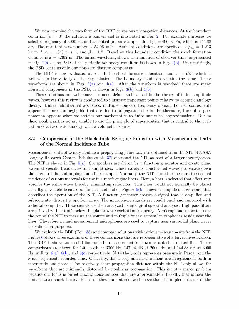
We have surveyed mathematically the relation between the Fay (Eqn. 21) and Fubini (Eqn. 29)solutions and the BBF (Eqn. 33) with governing equations. Here, we will illustrate their physicalsignificance graphically. Figure 1 shows the amplitudes of the three solutions as a function of non-dimensional distance from a sinusoidal boundary condition. The contribution of Fay (Eqn. 21) isshown as a dashed line with squares, the contribution of Fubini (Eqn. 29) is shown as a dash-dotline with triangles, and the BBF (Eqn. 33) is shown as a solid line. The amplitudes are normalizedwith respect to the amplitude of the source at σ = 0. Recall that σ = xx−1. The amplitude iscalculated numerically by summing the Fourier coefficient magnitudes over all frequencies at eachspatial position. Due to the assumptions and method of solution of Fubini (Eqn. 29), the Fubinisolution is valid from 0 ≤ σ < 1. It immediately decays and approaches zero as the limit σ → ∞.Fay, who sought stable waveforms, shows a valid solution for σ > 3.5 until viscous effects dominatethe dynamics of wave propagation. Within the region 1 ≤ σ < 3.5 neither the Fay or Fubini solutionare correct. The BBF bridges the two solutions and satisfies (at least to engineering accuracy) thegeneralized Burger’s equation.

13

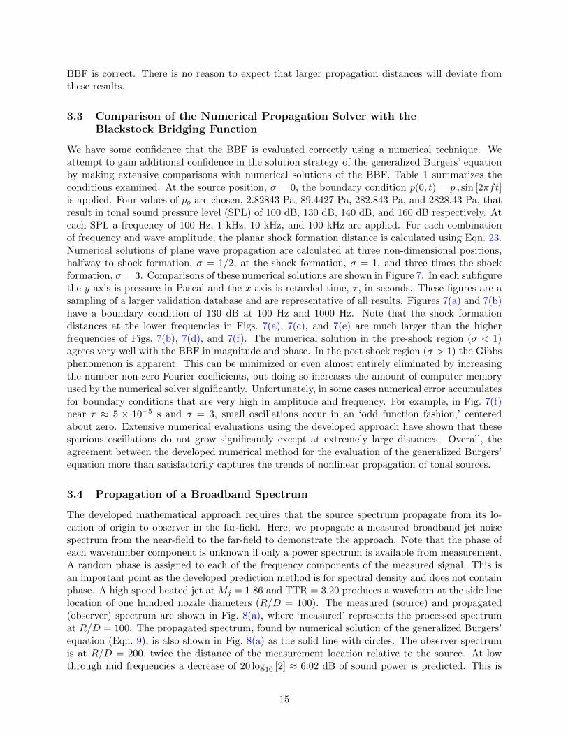
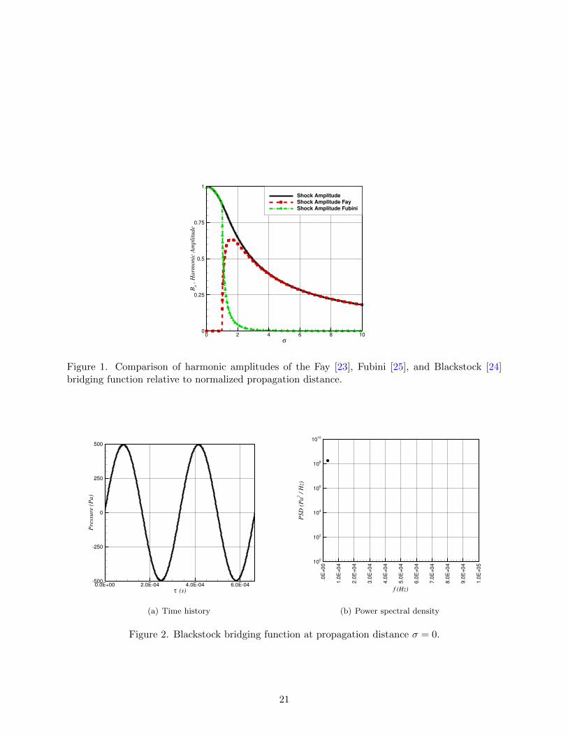
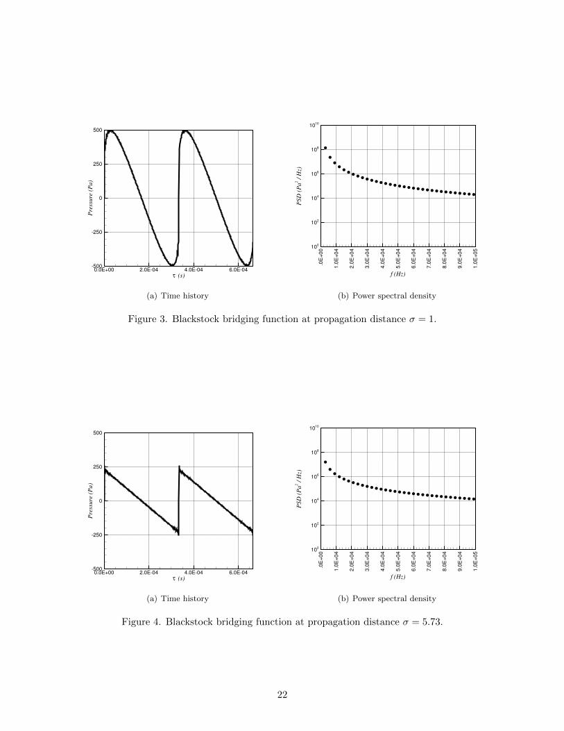
We now examine the waveform of the BBF at various propagation distances. At the boundarycondition (σ = 0) the solution is known and is illustrated in Fig. 2. For example purposes weselect a frequency of 3000 Hz and an initial pressure amplitude of po = 496.07 Pa, which is 144.88dB. The resultant wavenumber is 54.96 m−1. Ambient conditions are specified as ρ∞ = 1.213kg m−3, c∞ = 343 m s−1, and β = 1.2. Based on this boundary condition the shock formationdistance is x = 4.362 m. The initial waveform, shown as a function of observer time, is presentedin Fig. 2(a). The PSD of the periodic boundary condition is shown in Fig. 2(b). Unsurprisingly,the PSD contains only one non-zero discrete component.

The BBF is now evaluated at σ = 1, the shock formation location, and σ = 5.73, which iswell within the validity of the Fay solution. The boundary condition remains the same. Thesewaveforms are shown in Figs. 3(a) and 4(a). After the waveform is ‘shocked’ there are manynon-zero components in the PSD, as shown in Figs. 3(b) and 4(b).

These solutions are well known to acousticians well versed in the theory of finite amplitudewaves, however this review is conducted to illustrate important points relative to acoustic analogytheory. Unlike infinitesimal acoustics, multiple non-zero frequency domain Fourier componentsappear that are non-negligible that are due to propagation effects. Furthermore, the Gibbs phe-nomenon appears when we restrict our mathematics to finite numerical approximations. Due tothese nonlinearities we are unable to use the principle of superposition that is central to the eval-uation of an acoustic analogy with a volumetric source.

3.2 Comparison of the Blackstock Bridging Function with Measurement Dataof the Normal Incidence Tube

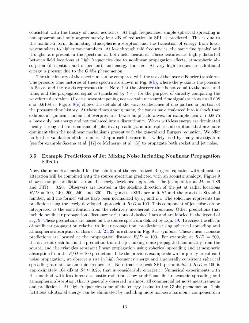
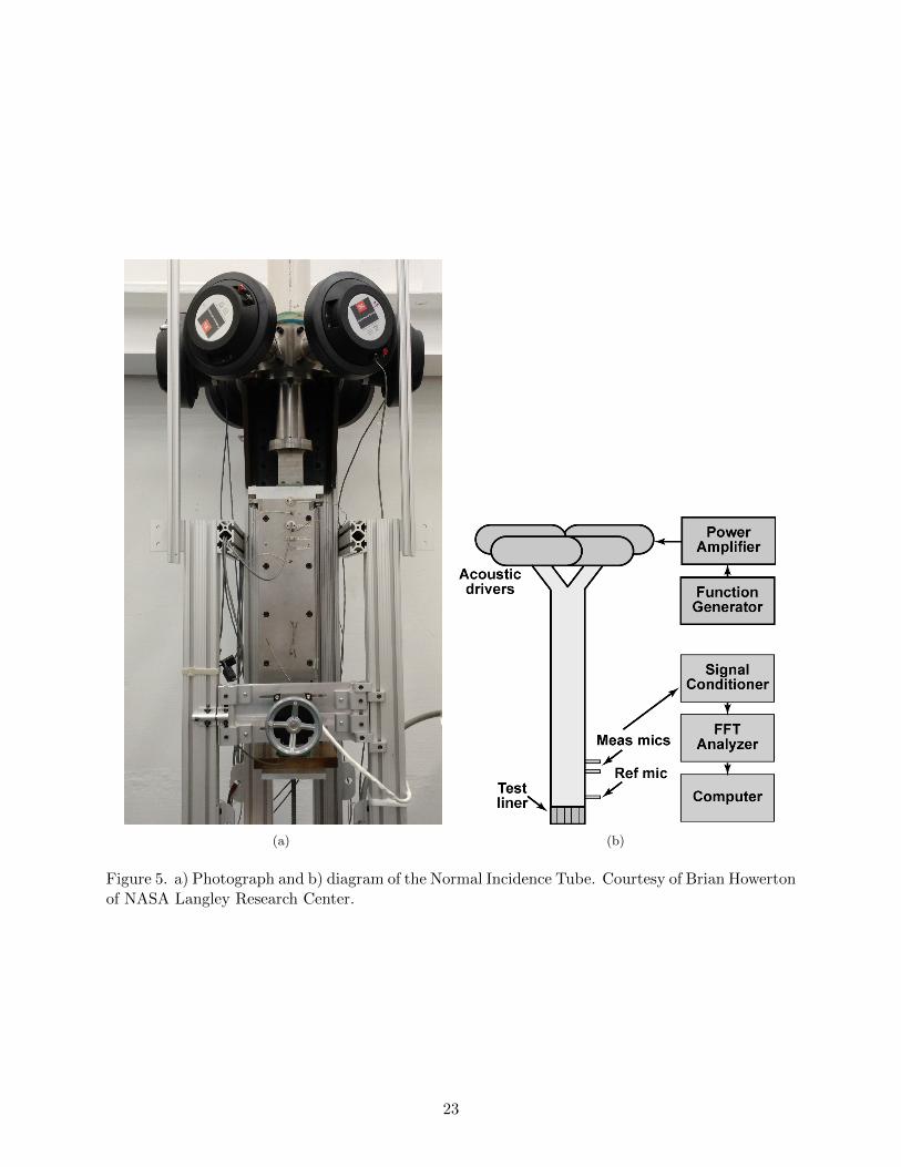
Measurement data of weakly nonlinear propagating plane waves is obtained from the NIT of NASALangley Research Center. Schultz et al. [32] discussed the NIT as part of a larger investigation.The NIT is shown in Fig. 5(a). Six speakers are driven by a function generator and create planewaves at specific frequencies and amplitudes. These carefully constructed waves propagate downthe circular tube and impinge on a liner sample. Normally, the NIT is used to measure the normalincidence of various materials for use in aircraft engine liners. Here, a liner is selected that effectivelyabsorbs the entire wave thereby eliminating reflection. This liner would not normally be placedin a flight vehicle because of its size and bulk. Figure 5(b) shows a simplified flow chart thatdescribes the operation of the NIT. A function generator creates a signal that is amplified andsubsequently drives the speaker array. The microphone signals are conditioned and captured witha digital computer. These signals are then analyzed using digital spectral analysis. High pass filtersare utilized with cut-offs below the planar wave excitation frequency. A microphone is located nearthe top of the NIT to measure the source and multiple ‘measurement’ microphones reside near theliner. The reference and measurement microphones are used to capture near sinusoidal plane wavesfor validation purposes.

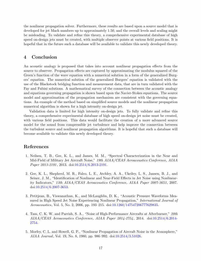
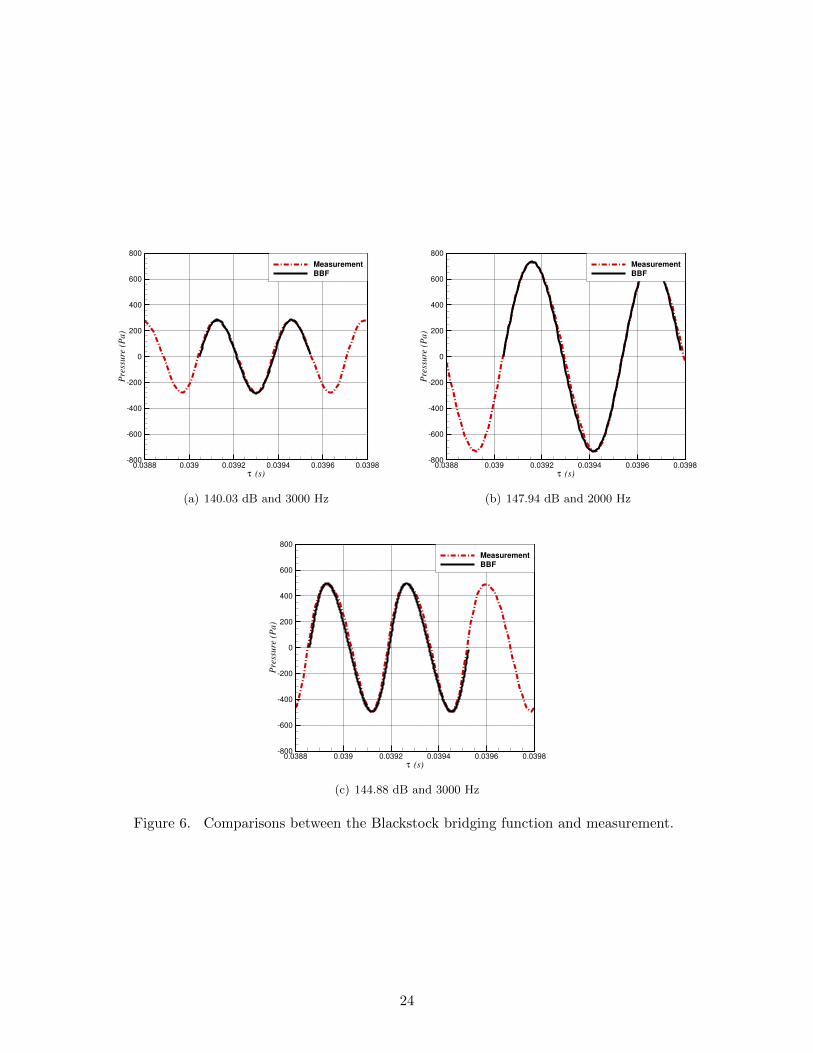
We evaluate the BBF (Eqn. 33) and compare solutions with various measurements from the NIT.Figure 6 shows three examples of these comparisons that are representative of a larger investigation.The BBF is shown as a solid line and the measurement is shown as a dashed-dotted line. Threecomparisons are shown for 140.03 dB at 3000 Hz, 147.94 dB at 2000 Hz, and 144.88 dB at 3000Hz, in Figs. 6(a), 6(b), and 6(c) respectively. Note the y-axis represents pressure in Pascal and thex-axis represents retarded time. Generally, this theory and measurement are in agreement both inmagnitude and phase. The relatively short propagation distance within the NIT only allows forwaveforms that are minimally distorted by nonlinear propagation. This is not a major problembecause our focus is on jet mixing noise sources that are approximately 165 dB, that is near thelimit of weak shock theory. Based on these validations, we believe that the implementation of the

14

BBF is correct. There is no reason to expect that larger propagation distances will deviate fromthese results.

3.3 Comparison of the Numerical Propagation Solver with theBlackstock Bridging Function

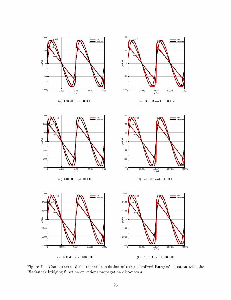
We have some confidence that the BBF is evaluated correctly using a numerical technique. Weattempt to gain additional confidence in the solution strategy of the generalized Burgers’ equationby making extensive comparisons with numerical solutions of the BBF. Table 1 summarizes theconditions examined. At the source position, σ = 0, the boundary condition p(0, t) = po sin [2πft]is applied. Four values of po are chosen, 2.82843 Pa, 89.4427 Pa, 282.843 Pa, and 2828.43 Pa, thatresult in tonal sound pressure level (SPL) of 100 dB, 130 dB, 140 dB, and 160 dB respectively. Ateach SPL a frequency of 100 Hz, 1 kHz, 10 kHz, and 100 kHz are applied. For each combinationof frequency and wave amplitude, the planar shock formation distance is calculated using Eqn. 23.Numerical solutions of plane wave propagation are calculated at three non-dimensional positions,halfway to shock formation, σ = 1/2, at the shock formation, σ = 1, and three times the shockformation, σ = 3. Comparisons of these numerical solutions are shown in Figure 7. In each subfigurethe y-axis is pressure in Pascal and the x-axis is retarded time, τ , in seconds. These figures are asampling of a larger validation database and are representative of all results. Figures 7(a) and 7(b)have a boundary condition of 130 dB at 100 Hz and 1000 Hz. Note that the shock formationdistances at the lower frequencies in Figs. 7(a), 7(c), and 7(e) are much larger than the higherfrequencies of Figs. 7(b), 7(d), and 7(f). The numerical solution in the pre-shock region (σ < 1)agrees very well with the BBF in magnitude and phase. In the post shock region (σ > 1) the Gibbsphenomenon is apparent. This can be minimized or even almost entirely eliminated by increasingthe number non-zero Fourier coefficients, but doing so increases the amount of computer memoryused by the numerical solver significantly. Unfortunately, in some cases numerical error accumulatesfor boundary conditions that are very high in amplitude and frequency. For example, in Fig. 7(f)near τ ≈ 5 × 10−5 s and σ = 3, small oscillations occur in an ‘odd function fashion,’ centeredabout zero. Extensive numerical evaluations using the developed approach have shown that thesespurious oscillations do not grow significantly except at extremely large distances. Overall, theagreement between the developed numerical method for the evaluation of the generalized Burgers’equation more than satisfactorily captures the trends of nonlinear propagation of tonal sources.

3.4 Propagation of a Broadband Spectrum

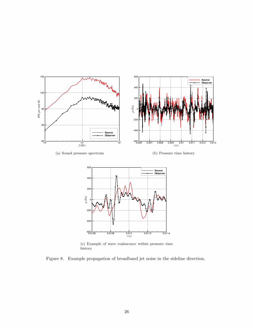
The developed mathematical approach requires that the source spectrum propagate from its lo-cation of origin to observer in the far-field. Here, we propagate a measured broadband jet noisespectrum from the near-field to the far-field to demonstrate the approach. Note that the phase ofeach wavenumber component is unknown if only a power spectrum is available from measurement.A random phase is assigned to each of the frequency components of the measured signal. This isan important point as the developed prediction method is for spectral density and does not containphase. A high speed heated jet at Mj = 1.86 and TTR = 3.20 produces a waveform at the side linelocation of one hundred nozzle diameters (R/D = 100). The measured (source) and propagated(observer) spectrum are shown in Fig. 8(a), where ‘measured’ represents the processed spectrumat R/D = 100. The propagated spectrum, found by numerical solution of the generalized Burgers’equation (Eqn. 9), is also shown in Fig. 8(a) as the solid line with circles. The observer spectrumis at R/D = 200, twice the distance of the measurement location relative to the source. At lowthrough mid frequencies a decrease of 20 log10 [2] ≈ 6.02 dB of sound power is predicted. This is

15

consistent with the theory of linear acoustics. At high frequencies, simple spherical spreading isnot apparent and only approximately four dB of reduction in SPL is predicted. This is due tothe nonlinear term dominating atmospheric absorption and the transition of energy from lowerwavenumbers to higher wavenumbers. At low through mid frequencies, the same fine ‘peaks’ and‘troughs’ are present in the spectrum at both field locations. These features are highly distortedbetween field locations at high frequencies due to nonlinear propagation effects, atmospheric ab-sorption (dissipation and dispersion), and energy transfer. At very high frequencies additionalenergy is present due to the Gibbs phenomenon.

The time history of the spectrum can be compared with the use of the inverse Fourier transform.The pressure time histories of these spectra are shown in Fig. 8(b), where the y-axis is the pressurein Pascal and the x-axis represents time. Note that the observer time is not equal to the measuredtime, and the propagated signal is translated by t − τ for the purpose of directly comparing thewaveform distortion. Observe wave steepening near certain measured time signals such as t ≈ 0.608s or 0.6108 s. Figure 8(c) shows the details of the wave coalescence of one particular portion ofthe pressure time history. At these times among many, the waves have coalesced into a shock thatexhibits a significant amount of overpressure. Lower amplitude waves, for example near t ≈ 0.6075s, have only lost energy and not coalesced into a discontinuity. Waves with less energy are dominatedlocally through the mechanisms of spherical spreading and atmospheric absorption, that are moredominant than the nonlinear mechanisms present with the generalized Burgers’ equation. We offerno further validation of this numerical approach because it is widely used by many investigators(see for example Saxena et al. [17] or McInerny et al. [6]) to propagate both rocket and jet noise.

3.5 Example Predictions of Jet Mixing Noise Including Nonlinear PropagationEffects

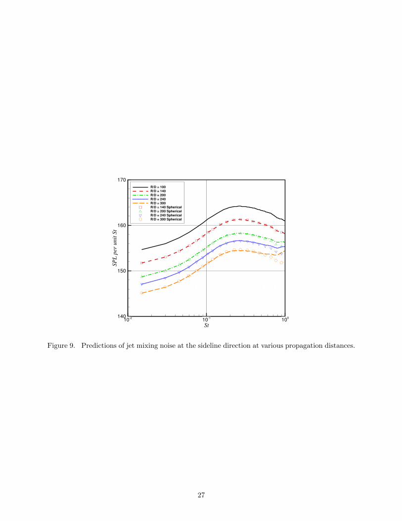
Now, the numerical method for the solution of the generalized Burgers’ equation with almost noalteration will be combined with the source spectrum predicted with an acoustic analogy. Figure 9shows example predictions from the newly developed approach. The jet operates at Mj = 1.86and TTR = 3.20. Observers are located in the sideline direction of the jet at radial locationsR/D = 100, 140, 200, 240, and 300. The y-axis is SPL per unit St and the x-axis is Strouhalnumber, and the former values have been normalized by uj and Dj . The solid line represents theprediction using the newly developed approach at R/D = 100. This component of jet noise can beinterpreted as the contribution from the relatively incoherent turbulence. Other predictions thatinclude nonlinear propagation effects are variations of dashed lines and are labeled in the legend ofFig. 9. These predictions are based on the source spectrum defined by Eqn. 49. To assess the effectsof nonlinear propagation relative to linear propagation, predictions using spherical spreading andatmospheric absorption of Bass et al. [21,22] are shown in Fig. 9 as symbols. These linear acousticpredictions are located at the propagation distance R/D = 100. For example, at R/D = 200,the dash-dot-dash line is the prediction from the jet mixing noise propagated nonlinearly from thesource, and the triangles represent linear propagation using spherical spreading and atmosphericabsorption from the R/D = 100 prediction. Like the previous example shown for purely broadbandnoise propagation, we observe a rise in high frequency energy and a generally consistent sphericalspreading rate at low and mid frequencies. Note that the peak SPL per unit St at R/D = 100 isapproximately 164 dB at St ≈ 0.25, that is considerably energetic. Numerical experiments withthis method with less intense acoustic radiation show traditional linear acoustic spreading andatmospheric absorption, that is generally observed in almost all commercial jet noise measurementsand predictions. At high frequencies some of the energy is due to the Gibbs phenomenon. Thisfictitious additional energy can be eliminated by including more non-zero harmonic components in

16

the nonlinear propagation solver. Furthermore, these results are based upon a source model that isdeveloped for jet Mach numbers up to approximately 1.50, and the overall levels and scaling mightbe misleading. To validate and refine this theory, a comprehensive experimental database of highspeed on-design jets must be created, with multiple observer points at various field positions. It ishopeful that in the future such a database will be available to validate this newly developed theory.

4 Conclusion

An acoustic analogy is proposed that takes into account nonlinear propagation effects from thesource to observer. Propagation effects are captured by approximating the modulus squared of theGreen’s function of the wave equation with a numerical solution in a form of the generalized Burg-ers’ equation. The numerical solution of the generalized Burgers’ equation is validated with theuse of the Blackstock bridging function and measurement data, that are in turn validated with theFay and Fubini solutions. A mathematical survey of the connection between the acoustic analogyand equations governing propagation is shown based upon the Navier-Stokes equations. The sourcemodel and approximation of the propagation mechanism are consistent with the governing equa-tions. An example of the method based on simplified source models and the nonlinear propagationnumerical algorithm is shown for a high intensity on-design jet.

Validation data is limited for high intensity on-design jets. To fully validate and refine thistheory, a comprehensive experimental database of high speed on-design jet noise must be created,with various field positions. This data would facilitate the creation of a more advanced sourcemodel for the sound from compressible jet turbulence and help improve the connection betweenthe turbulent source and nonlinear propagation algorithms. It is hopeful that such a database willbecome available to validate this newly developed theory.

References

1. Neilsen, T. B., Gee, K. L., and James, M. M., “Spectral Characterization in the Near andMid-Field of Military Jet Aircraft Noise,” 19th AIAA/CEAS Aeroacoustics Conference, AIAAPaper 2013-2191 , 2013. doi:10.2514/6.2013-2191.

2. Gee, K. L., Shepherd, M. R., Falco, L. E., Atchley, A. A., Ukeiley, L. S., Jansen, B. J., andSeiner, J. M., “Identification of Nonlinear and Near-Field Effects in Jet Noise using Nonlinear-ity Indicators,” 13th AIAA/CEAS Aeroacoustics Conference, AIAA Paper 2007-3653 , 2007.doi:10.2514/6.2007-3653.

3. Petitjean, B., Viswanathan, K., and McLaughlin, D. K., “Acoustic Pressure Waveforms Mea-sured in High Speed Jet Noise Experiencing Nonlinear Propagation,” International Journal ofAeroacoustics, Vol. 5, No. 2, 2006, pp. 193–215. doi:10.1260/147547206777629835.

4. Tam, C. K. W. and Parrish, S. A., “Noise of High-Performance Aircrafts at Afterburner,” 20thAIAA/CEAS Aeroacoustics Conference, AIAA Paper 2014-2754 , 2014. doi:10.2514/6.2014-2754.

5. Morfey, C. L. and Howell, G. P., “Nonlinear Propagation of Aircraft Noise in the Atmosphere,”AIAA Journal , Vol. 19, No. 8, 1980, pp. 986–992. doi:10.2514/3.51026.

17

6. McInerny, S. A. and Olcmen, S. M., “High-Intensity Rocket Noise: Nonlinear Propagation,Atmospheric Absorption, and Characterization,” Journal of the Acoustical Society of America,Vol. 117, No. 2, 2005, pp. 578–591. doi:10.1121/1.1841711.

7. Gee, K. L., Giraud, J. H., Blotter, J. D., and Sommerfeldt, S. D., “Energy-Based AcousticalMeasurements of Rocket Noise,” 15th AIAA/CEAS Aeroacoustics Conference, AIAA Paper2009-3165 , 2009. doi:10.2514/6.2009-3165.

8. Lighthill, M. J., “On Sound Generated Aerodynamically. I. General Theory,” Proc. R. Soc.Lond. A., Vol. 211, No. 1107, 1952, pp. 564–587. doi:10.1098/rspa.1952.0060.

9. Miller, S. A. E., “Prediction of Near-Field Jet Cross Spectra,” AIAA Journal , 2015.doi:10.2514/1.J053614.

10. Schlichting, H. and Gersten, K., “Boundary-Layer Theory,” Springer-Verlag, New York , 2000.

11. Crighton, D. G., “Model Equations of Nonlinear Acoustics,” Annual Review of Fluid Mechanics,Vol. 11, 1979, pp. 11–33. doi:10.1146/annurev.fl.11.010179.000303.

12. Blackstock, D. T., “Generalized Burgers Equation for Plane Waves,” Journal of the AcousticalSociety of America, Vol. 77, No. 6, 1985, pp. 2050–2053. doi:10.1121/1.391778.

13. Blackstock, D. T., “History of Nonlinear Acoustics and a Survey of Burgers and Related Equa-tions,” Proceedings of a Conference held at the Applied Research Laboratories, The Universityof Texas at Austin, 1969, pp. 1–27.

14. Vladimirov, V. A. and Maczka, C., “Exact Solutions of Generalized Burgers Equation, De-scribing Travelling Fronts and Their Interaction,” Reports on Mathematical Physics, Vol. 60,No. 2, 2007, pp. 317–328. doi:10.1016/S0034-4877(07)80142-X.

15. Mendousse, J. S., “Nonlinear Dissipative Distortion of Progressive Sound Waves at ModerateAmplitudes,” Journal of the Acoustical Society of America, Vol. 25, No. 51, 1953, pp. 51–54.doi:10.1121/1.1907007.

16. Lighthill, M. J., “Viscosity Effects in Sound Waves of Finite Amplitude,” Surveys in Mechanics,Cambridge University Press (Davies R. M. and Batchelor, G. K. (Eds.)), 1956, pp. 250–351.

17. Saxena, S., Morris, P. J., and Viswanathan, K., “Algorithm for the Nonlinear Propaga-tion of Broadband Jet Noise,” AIAA Journal , Vol. 47, No. 186-194, 2009, pp. 186–194.doi:10.2514/1.38122.

18. Lee, S. L., Morris, P. J., and Brentner, K. S., “Improved Algorithm for Nonlinear SoundPropagation with Aircraft and Helicopter Noise Applications,” AIAA Journal , Vol. 48, No. 11,2010, pp. 2586–2595. doi:10.2514/1.J050396.

19. Saxena, S., “A New Algorithm for Nonlinear Propagation of Broadband Jet Noise,” M.S.Thesis, The Pennsylvania State University , 2008.

20. Duchon, C. E., “Lanczos Filtering in One and Two Dimensions,” Journal of Applied Meteorol-ogy , Vol. 18, No. 8, 1979, pp. 1016–1022.

21. Bass, H. E., Sutherland, L. C., Zuckerwar, A. J., Blackstock, T. D., and Hester, D. M., “At-mospheric Absorption of Sound: Further Developments,” Journal of the Acoustical Society ofAmerica, Vol. 97, No. 1, 1995, pp. 680–683. doi:10.1121/1.412989.

18

22. Bass, H. E., Sutherland, L. C., Zuckerwar, A. J., Blackstock, T. D., and Hester, D. M., “Er-ratum: Atmospheric Absorption of Sound: Further Developments,” Journal of the AcousticalSociety of America, Vol. 99, No. 2, 1995, pp. 1259–1259. doi:10.1121/1.415223.

23. Fay, R. D., “Plane Sound Waves of Finite Amplitude,” Journal of the Acoustical Society ofAmerica, Vol. 3, No. 9, 1931, pp. 222–241. doi:10.1121/1.1901928.

24. Blackstock, D. T., “Connection Between the Fay and Fubini Solutions for Plane Sound Wavesof Finite Amplitude,” Journal of the Acoustical Society of America, Vol. 39, No. 6, 1965,pp. 1019–1026. doi:10.1121/1.1909986.

25. Fubini-Ghiron, E., “Anomalie nella Propagazione di onde Acustiche di Grande Ampiezza,” AltaFrequenza, Vol. 4, 1935, pp. 530–581.

26. Westervelt, P. J., “The Mean Pressure and Velocity in a Plane Acoustic Wave in a Gas,”The Journal of the Acoustical Society of America, Vol. 22, No. 3, 1950, pp. 319–327.doi:10.1121/1.1906606.

27. Earnshaw, S., “On the Mathematical Theory of Sound,” Phil. Trans. R. Soc. London, Vol. 150,1860, pp. 133–148. doi:10.1098/rstl.1860.0009.

28. Ffowcs Williams, J. E., “The Noise from Turbulence Convected at High Speed,” Phil. Trans.R. Soc. Lond. A, Vol. 255, No. 1063, 1963, pp. 469–503. doi:10.1098/rsta.1963.0010.

29. Lau, J. C., Morris, P. J., and Fisher, M. J., “Measurements in Subsonic and Supersonic FreeJets using a Laser Velocimeter,” Journal of Fluid Mechanics, Vol. 93, No. 1, 1979, pp. 1–27.doi:10.1017/S0022112079001750.

30. Lau, J. C., Morris, P. J., and Fisher, M. J., “Effects of Exit Mach Number and Temperatureon Mean-Flow and Turbulence Characteristics in Round Jets,” Journal of Fluid Mechanics,Vol. 105, No. 1, 1981, pp. 193–218. doi:10.1017/S0022112081003170.

31. Tam, C. K. W., “Broadband Shock-Associated Noise of Moderately Imperfectly ExpandedJets,” Journal of Sound and Vibration, Vol. 140, No. 1, 1990, pp. 55–71. doi:10.1016/0022-460X(90)90906-G.

32. Schultz, T., Liu, F., Cattafesta, L., Sheplak, M., and Jones, M., “A Comparison Study ofNormal-Incidence Acoustic Impedance Measurements of a Perforate Liner,” 15th AIAA/CEASAeroacoustics Conference, AIAA Paper 2009-3301 , 2009. doi:10.2514/6.2009-3301.

19

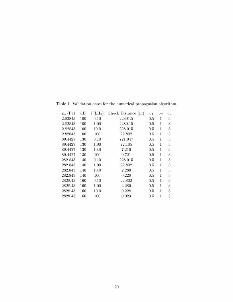
Table 1. Validation cases for the numerical propagation algorithm.

po (Pa) dB f (kHz) Shock Distance (m) σ1 σ2 σ2

2.82843 100 0.10 22801.5 0.5 1 32.82843 100 1.00 2280.15 0.5 1 32.82843 100 10.0 228.015 0.5 1 32.82843 100 100 22.802 0.5 1 389.4427 130 0.10 721.047 0.5 1 389.4427 130 1.00 72.105 0.5 1 389.4427 130 10.0 7.210 0.5 1 389.4427 130 100 0.721 0.5 1 3282.843 140 0.10 228.015 0.5 1 3282.843 140 1.00 22.802 0.5 1 3282.843 140 10.0 2.280 0.5 1 3282.843 140 100 0.228 0.5 1 32828.43 160 0.10 22.802 0.5 1 32828.43 160 1.00 2.280 0.5 1 32828.43 160 10.0 0.228 0.5 1 32828.43 160 100 0.023 0.5 1 3

20

σ

Bn ,

Ha

rmon

ic A

mp

litu

de

0 2 4 6 8 100

0.25

0.5

0.75

1

Shock AmplitudeShock Amplitude Fay

Shock Amplitude Fubini

Figure 1. Comparison of harmonic amplitudes of the Fay [23], Fubini [25], and Blackstock [24]bridging function relative to normalized propagation distance.

τ (s)

Pre

ssu

re (

Pa

)

0.0E+00 2.0E­04 4.0E­04 6.0E­04­500

­250

0

250

500

(a) Time history

f (Hz)

PS

D (

Pa

2 /

Hz)

.0E

+0

0

1.0

E+

04

2.0

E+

04

3.0

E+

04

4.0

E+

04

5.0

E+

04

6.0

E+

04

7.0

E+

04

8.0

E+

04

9.0

E+

04

1.0

E+

05

100

102

104

106

108

1010

(b) Power spectral density

Figure 2. Blackstock bridging function at propagation distance σ = 0.

21

τ (s)

Pre

ssu

re (

Pa

)

0.0E+00 2.0E­04 4.0E­04 6.0E­04­500

­250

0

250

500

(a) Time history

f (Hz)

PS

D (

Pa

2 /

Hz)

.0E

+0

0

1.0

E+

04

2.0

E+

04

3.0

E+

04

4.0

E+

04

5.0

E+

04

6.0

E+

04

7.0

E+

04

8.0

E+

04

9.0

E+

04

1.0

E+

05

100

102

104

106

108

1010

(b) Power spectral density

Figure 3. Blackstock bridging function at propagation distance σ = 1.

τ (s)

Pre

ssu

re (

Pa

)

0.0E+00 2.0E­04 4.0E­04 6.0E­04­500

­250

0

250

500

(a) Time history

f (Hz)

PS

D (

Pa

2 /

Hz)

.0E

+0

0

1.0

E+

04

2.0

E+

04

3.0

E+

04

4.0

E+

04

5.0

E+

04

6.0

E+

04

7.0

E+

04

8.0

E+

04

9.0

E+

04

1.0

E+

05

100

102

104

106

108

1010

(b) Power spectral density

Figure 4. Blackstock bridging function at propagation distance σ = 5.73.

22

(a) (b)

Figure 5. a) Photograph and b) diagram of the Normal Incidence Tube. Courtesy of Brian Howertonof NASA Langley Research Center.

23

τ (s)

Pre

ssu

re (

Pa

)

0.0388 0.039 0.0392 0.0394 0.0396 0.0398­800

­600

­400

­200

0

200

400

600

800

Measurement

BBF

(a) 140.03 dB and 3000 Hz

τ (s)

Pre

ssu

re (

Pa

)

0.0388 0.039 0.0392 0.0394 0.0396 0.0398­800

­600

­400

­200

0

200

400

600

800

Measurement

BBF

(b) 147.94 dB and 2000 Hz

τ (s)

Pre

ssu

re (

Pa

)

0.0388 0.039 0.0392 0.0394 0.0396 0.0398­800

­600

­400

­200

0

200

400

600

800

Measurement

BBF

(c) 144.88 dB and 3000 Hz

Figure 6. Comparisons between the Blackstock bridging function and measurement.

24

τ (s)

p (

Pa

)

0 0.005 0.01 0.015 0.02­100

­50

0

50

100

BBF

Prediction

σ=0.5

σ=1.0

σ=3.0

(a) 130 dB and 100 Hz

τ (s)

p (

Pa

)

0 0.0005 0.001 0.0015 0.002­100

­50

0

50

100

BBF

Prediction

σ=0.5

σ=1.0

σ=3.0

(b) 130 dB and 1000 Hz

τ (s)

p (

Pa

)

0 0.005 0.01 0.015 0.02­300

­200

­100

0

100

200

300

BBF

Prediction

=0.5

σ=1.0

=3.0

(c) 140 dB and 100 Hz

τ (s)

p (

Pa

)

0 5E­05 0.0001 0.00015 0.0002­300

­200

­100

0

100

200

300

BBF

Prediction

=0.5

σ=1.0

=3.0

(d) 140 dB and 10000 Hz

τ (s)

p (

Pa

)

0 0.0005 0.001 0.0015 0.002­3000

­2000

­1000

0

1000

2000

3000

BBF

Prediction

=0.5

σ=1.0

σ=3.0

(e) 160 dB and 1000 Hz

τ (s)

p (

Pa

)

0 5E­05 0.0001 0.00015 0.0002­3000

­2000

­1000

0

1000

2000

3000

BBF

Prediction

=0.5

σ=1.0

σ=3.0

(f) 160 dB and 10000 Hz

Figure 7. Comparisons of the numerical solution of the generalized Burgers’ equation with theBlackstock bridging function at various propagation distances σ.

25

f (Hz)

SP

L p

er u

nit

Hz

102

103

10485

90

95

100

105

Source

Observer

(a) Sound pressure spectrum

t (s)

p (

Pa

)

0.606 0.607 0.608 0.609 0.61 0.611 0.612 0.613­600

­400

­200

0

200

400

600

Source

Observer

(b) Pressure time history

t (s)

p (

Pa

)

0.6106 0.6108 0.611 0.6112 0.6114­600

­400

­200

0

200

400

600

Source

Observer

(c) Example of wave coalescence within pressure timehistory

Figure 8. Example propagation of broadband jet noise in the sideline direction.

26

St

SP

L p

er u

nit

St

10­2

10­1

100140

150

160

170

R/D = 100

R/D = 140

R/D = 200

R/D = 240

R/D = 300

R/D = 140 Spherical

R/D = 200 Spherical

R/D = 240 Spherical

R/D = 300 Spherical

Figure 9. Predictions of jet mixing noise at the sideline direction at various propagation distances.

27

REPORT DOCUMENTATION PAGEForm Approved

OMB No. 0704-0188

2. REPORT TYPE

Technical Memorandum 4. TITLE AND SUBTITLE

Toward a Nonlinear Acoustic Analogy: Turbulence as a Source of Sound and Nonlinear Propagation

5a. CONTRACT NUMBER

6. AUTHOR(S)

Miller, Steven A. E.

7. PERFORMING ORGANIZATION NAME(S) AND ADDRESS(ES)

NASA Langley Research CenterHampton, VA 23681-2199

9. SPONSORING/MONITORING AGENCY NAME(S) AND ADDRESS(ES)

National Aeronautics and Space AdministrationWashington, DC 20546-0001

8. PERFORMING ORGANIZATION REPORT NUMBER

L-20532

10. SPONSOR/MONITOR'S ACRONYM(S)

NASA

13. SUPPLEMENTARY NOTES

12. DISTRIBUTION/AVAILABILITY STATEMENTUnclassified - UnlimitedSubject Category 71Availability: NASA STI Program (757) 864-9658

19a. NAME OF RESPONSIBLE PERSON

STI Help Desk (email: help@sti.nasa.gov)

14. ABSTRACT

An acoustic analogy is proposed that directly includes nonlinear propagation effects. Here, we examine the Lighthill acoustic analogy and replace the Green's function of the wave equation with numerical solutions of the generalized Burgers' equation. This is justified mathematically by using similar arguments that are the basis of the solution of the Lighthill acoustic analogy. This approach is superior to alternatives because propagation is accounted for directly from the source to the far-field observer instead of from an arbitrary intermediate point. Validation of a numerical solver for the generalized Burgers' equation is performed by comparing solutions with the Blackstock bridging function and measurement data. Most importantly, the mathematical relationship between the Navier-Stokes equations, the acoustic analogy that describes the source, and canonical nonlinear propagation equations is shown. Finally, example predictions are presented for nonlinear propagation of jet mixing noise at the sideline angle. 15. SUBJECT TERMS

Acoustic analogy; Blackstock; Fay; Fubini; Green's function; Jet; Nonlinear; Propagation; Rocket; Turbulence

18. NUMBER OF PAGES

3219b. TELEPHONE NUMBER (Include area code)

(757) 864-9658

a. REPORT

U

c. THIS PAGE

U

b. ABSTRACT

U

17. LIMITATION OF ABSTRACT

UU

Prescribed by ANSI Std. Z39.18Standard Form 298 (Rev. 8-98)

3. DATES COVERED (From - To)

5b. GRANT NUMBER

5c. PROGRAM ELEMENT NUMBER

5d. PROJECT NUMBER

5e. TASK NUMBER

5f. WORK UNIT NUMBER

110076.02.07.04.01

11. SPONSOR/MONITOR'S REPORT NUMBER(S)

NASA-TM-2015-218706

16. SECURITY CLASSIFICATION OF:

The public reporting burden for this collection of information is estimated to average 1 hour per response, including the time for reviewing instructions, searching existing data sources, gathering and maintaining the data needed, and completing and reviewing the collection of information. Send comments regarding this burden estimate or any other aspect of this collection of information, including suggestions for reducing this burden, to Department of Defense, Washington Headquarters Services, Directorate for Information Operations and Reports (0704-0188), 1215 Jefferson Davis Highway, Suite 1204, Arlington, VA 22202-4302. Respondents should be aware that notwithstanding any other provision of law, no person shall be subject to any penalty for failing to comply with a collection of information if it does not display a currently valid OMB control number.PLEASE DO NOT RETURN YOUR FORM TO THE ABOVE ADDRESS.

1. REPORT DATE (DD-MM-YYYY)

04 - 201501-