Embed Size (px)
Citation preview

Toward a theory of monopolistic competition
⇤
Mathieu Parenti† Philip Ushchev‡ Jacques-François Thisse§
August 19, 2014
Abstract
We propose a general model of monopolistic competition, which encompasses existing models
while being flexible enough to take into account new demand and competition features. The basic
tool we use to study the market outcome is the elasticity of substitution at a symmetric consumption
pattern, which depends on both the per capita consumption and the total mass of varieties. We
impose intuitive conditions on this function to guarantee the existence and uniqueness of a free-entry
equilibrium. Comparative statics with respect to population size, GDP per capita and productivity
shock are characterized through necessary and sufficient conditions. Finally, we show how our approach
can be generalized to the case of a multisector economy and extended to cope with heterogeneous firms
and consumers.
Keywords: monopolistic competition, general equilibrium, additive preferences, homothetic pref-erences
JEL classification: D43, L11, L13.
⇤We are grateful to C. d’Aspremont, K. Behrens, A. Costinot, F. Di Comite, R. Dos Santos, S. Kichko, H. Konishi,V. Ivanova, P. Legros, M.-A. López García, O. Loginova , Y. Murata, G. Ottaviano, J. Tharakan and seminaraudience at Bologna U., CEFIM, ECORES, E.I.E.F., Lille 1, NES, Stockholm U., UABarcelona, and UQAMontréalfor comments and suggestions. We owe special thanks to A. Savvateev for discussions about the application offunctional analysis to the consumer problem. We acknowledge the financial support from the Government of theRussian Federation under the grant 11.G34.31.0059.
†CORE-UCLouvain (Belgium) and NRU-Higher School of Economics (Russia). Email: [email protected]
‡NRU-Higher School of Economics (Russia). Email: [email protected]§CORE-UCLouvain (Belgium), NRU-Higher School of Economics (Russia) and CEPR. Email:
1
1 Introduction
The theory of general equilibrium with imperfectly competitive markets is still in infancy. In hissurvey of the various attempts made in the 1970s and 1980s to integrate oligopolistic competitionwithin the general equilibrium framework, Hart (1985) has convincingly argued that these contri-butions have failed to produce a consistent and workable model. Unintentionally, the absence of ageneral equilibrium model of oligopolistic competition has paved the way to the success of the CESmodel of monopolistic competition developed by Dixit and Stiglitz (1977). And indeed, the CESmodel has been used in so many economic fields that a large number of scholars believe that thisis the model of monopolistic competition. For example, Head and Mayer (2014) observe that thismodel is “nearly ubiquitous” in the trade literature. However, owing to its extreme simplicity, theCES model dismisses several important effects that contradict basic findings in economic theory,as well as empirical evidence. To mention a few, unlike what the CES predicts, prices and firmsizes are affected by entry, market size and consumer income, while markups vary with costs.
In addition, tweaking the CES or using other specific models in the hope of obviating these dif-ficulties does not permit to check the robustness of the results. For example, quadratic preferencesare consistent with lower prices and higher average productivity in larger markets. By contrast,quadratic preferences imply that prices are independent of income, the reason being that they arenested in a quasi-linear utility. The effect of GDP per capita can be restored if preferences areindirectly additive, but then prices no longer depend on the number of competitors. If preferencesare CES and the market structure is oligopolistic, markups depend again on the number of firms,but no longer on the GDP per capita. In sum, it seems fair to say that the state of the art looks likea scattered field of incomplete and insufficiently related contributions in search of a more generalapproach.
Our purpose is to build a general equilibrium model of monopolistic competition that hasthe following two features. First, it encompasses all existing models of monopolistic competition.Second, it displays enough flexibility to take into account demand and competition attributes in away that will allow us to determine under which conditions many findings are valid. In this respect,we concur with Mrázová and Neary (2013) that “assumptions about the structure of preferencesand demand matter enormously for comparative statics.” This is why we consider a setting inwhich preferences are unspecified and characterize preferences through necessary and sufficientconditions for each comparative static effect to hold. This allows us to identify which findings holdtrue against alternative preference specifications, and those which depend on particular classesof preferences. This should be useful to the applied economists in discriminating between thedifferent specifications used in their settings. The flip side of the coin is the need to reduce thecomplexity of the problem. This is why, in the baseline model, we focus on competition amongsymmetric firms. We see this as a necessary step toward the development and analysis of a fullygeneral theory of monopolistic competition.
2

By modeling monopolistic competition as a noncooperative game with a continuum of players,we are able to obviate at least two major problems.1 First, we capture Chamberlin’s central ideaaccording to which the cross elasticities of demands are equal to zero, the reason being that eachfirm is negligible to the market. Second, whereas the redistribution of firms’ profits is at the rootof the non-existence of an equilibrium in general equilibrium with oligopolistic competition, we getrid of this feedback effect because individual firms are unable to manipulate profits. Thus, firmsdo not have to make full general equilibrium calculations before choosing their profit-maximizingstrategy. Admittedly, the continuum assumption may be viewed as a deus ex machina. But we endup with a consistent and analytically tractable model in which firms are bound together throughvariables that give rise to income and substitution effects in consumers’ demand. This has a far-fetched implication: even though firms do not compete strategically, our model is able to mimicoligopolistic markets and to generate within a general equilibrium framework findings akin to thoseobtained in partial equilibrium settings. As will be shown, the CES is the only case in which alleffects vanish.
Our main findings may be summarized as follows. First, using an extension of the concept ofdifferentiability to the case where the unknowns are functions rather than vectors, we determine ageneral demand system, which includes a wide range of special cases such as the CES, quadratic,CARA, additive, indirectly additive, and homothetic preferences. At any symmetric market out-come, the individual demand for a variety depends only upon its consumption when preferences areadditive. By contrast, when preferences are homothetic, the demand for a variety depends uponits relative consumption level and the mass of available varieties. Therefore, when preferences areneither additive nor homothetic, the demand for a variety must depend on its consumption leveland the total mass of available varieties.
Second, to prove the existence and uniqueness of a free-entry equilibrium and to study itsproperties, we need to impose some restrictions on the demand side of our model. Rather thanmaking new assumptions on preferences and demands, we tackle the problem from the viewpointof the theory of product differentiation. To be precise, the key concept of our model is the elasticityof substitution across varieties. We then exploit the symmetry of preferences over a continuum ofgoods to show that, under the most general specification of preferences, at any symmetric outcomethe elasticity of substitution between any two varieties is a function of two variables only: the pervariety consumption and the total mass of firms. Combining this with the absence of the business-stealing effect of oligopoly theory reveals that, at the market equilibrium, firms’ markup is equalto the inverse of the equilibrium value of the elasticity of substitution. This result agrees with oneof the main messages of industrial organization: the higher is the elasticity of substitution, the lessdifferentiated are varieties, and thus the lower are firms’ markup.
Therefore, it should be clear that the properties of the symmetric free-entry equilibrium depends1The idea of using a continuum of firms was proposed by Dixit and Stiglitz in their 1974 working paper, which
has been published in Brakman and Heijdra (2004)
3

on how the elasticity of substitution function behaves when the per variety consumption and themass of firms vary with the main parameters of the economy. This allows us to study the marketoutcome by means of simple analytical arguments. To be precise, by imposing plausible conditionsto the elasticity of substitution function, we are able to disentangle the various determinants offirms’ strategies. We will determine our preferred set of assumptions by building on what thetheory of product differentiation tells us, as well as on empirical evidence.
Third, to insulate the impact of various types of preferences on the market outcome, we focuson symmetric firms and, therefore, on symmetric free-entry equilibria. We provide necessary andsufficient conditions on the elasticity of substitution for the existence and uniqueness of a free-entryequilibrium. Our setting is especially well suited to conduct detailed comparative static analysesin that we can determine the necessary and sufficient conditions for all the thought experimentsundertaken in the literature. The most typical experiment is to study the impact of market size.What market size signifies is not always clear because it compounds two variables, i.e., the numberof consumers and their willingness-to-pay for the product under consideration. The impact ofpopulation size and income level on prices, output and the number of firms need not be the samebecause these two parameters affect firms’ demand in different ways. An increase in populationor in income raises demand, thereby fostering entry and lower prices. But an income hike alsoraises consumers’ willingness-to-pay, which tends to push prices upward. The final impact is thusa priori ambiguous.
We show that a larger market results in a lower market price and bigger firms if and only ifthe elasticity of substitution responds more to a change in the mass of varieties than to a changein the per variety consumption. This is so in the likely case where the entry of new firms doesnot render varieties much more differentiated. Regarding the mass of varieties, it increases withthe number of consumers if varieties do not become too similar when their number rises. Thus,like most oligopoly models, monopolistic competition exhibits the standard pro-competitive effectsassociated with market size and entry. However, anti-competitive effects cannot be ruled out apriori. Furthermore, an increase in individual income generates similar, but not identical, effectsif and only if varieties become closer substitutes when their range widens. The CES is the onlyutility for which price and output are independent of both income and market size.
Our setting also allows us to study the impact of a cost change on markups. When all firms facethe same productivity hike, we show that the nature of preferences determines the extent of thepass-through. Specifically, a decrease in marginal cost leads to a lower market price, but a highermarkup, if and only if the elasticity of substitution decreases with the per capita consumption. Inthis event, there is incomplete pass-through. However, the pass-through rate need not be smallerthan one.
Last, we discuss three major extensions of our baseline model. In the first one, we focuson Melitz-like heterogeneous firms. In this case, when preferences are non-additive, the profit-maximizing strategy of a firm depends directly on the strategies chosen by all the other types’ firms,
4

which vastly increases the complexity of the problem. Despite of this, we show that, regardless ofthe distribution of marginal costs, firms are sorted out by decreasing productivity order, while abigger market sustains a larger number of active firms. We highlight the role of the elasticity ofsubstitution by showing that it now depends on the number entrants and the cutoff costs for eachtype of firm. In the second, we consider a multisector economy. The main additional difficulty stemsfrom the fact that the sector-specific expenditures depend on the upper-tier utility. Under a fairlymild assumption on the marginal utility, we prove the existence of an equilibrium and show thatmany of our results hold true for the monopolistically competitive sector. This highlights the ideathat our model can be used as a building block to embed monopolistic competition in full-fledgedgeneral equilibrium models coping with various economic issues. Our last extension addressesthe almost untouched issue of consumer heterogeneity in love-for-variety models of monopolisticcompetition. Consumers may be heterogeneous because of taste and/or income differences. Here,we will restrict ourselves to special, but meaningful, cases.
Related literature. Different alternatives have been proposed to avoid the main pitfalls of theCES model. Behrens and Murata (2007) propose the CARA utility that captures both price andsize effects, while Zhelobodko et al. (2012) use general additive preferences to work with a variableelasticity of substitution, and thus variable markups. Bertoletti and Etro (2014) consider anadditive indirect utility function to study the impact of per capita income on the market outcome,but price and firm size are independent of population size. Vives (1999) and Ottaviano et al.(2002) show how the quadratic utility model obviates some of the difficulties associated with theCES model, while delivering a full analytical solution. Bilbiie et al. (2012) use general symmetrichomothetic preferences in a real business cycle model. Last, pursuing a different objective, Mrázováand Neary (2013) study a specific class of demand functions, that is, those which leaves therelationships between the elasticity and convexity of demands unchanged, and aim to predict thewelfare effects of a wide range of shocks.
In the next section, we describe the demand and supply sides of our setting. The primitive ofthe model being the elasticity of substitution function, we discuss in Section 3 how this functionmay vary with the per variety consumption and the mass of varieties. In Section 4, we prove theexistence and uniqueness of a free-entry equilibrium and characterize its various properties. Thethree extensions are discussed in Section 5, while Section 6 concludes.
2 The model and preliminary results
Consider an economy with a mass L of identical consumers, one sector and one production factor– labor, which is used as the numéraire. Each consumer is endowed with y efficiency units of labor,so that the per capita income y is given and the same across consumers because the unit wage is1. This will allow us to discriminate between the effects generated by the consumer income, y, and
5

the number of consumers, L. On the supply side, there is a continuum of firms producing each ahorizontally differentiated good under increasing returns. Each firm supplies a single variety andeach variety is supplied by a single firm.
2.1 Consumers
Let N , an arbitrarily large number, be the mass of “potential” varieties, e.g., the varieties for whicha patent exists. Very much like in the Arrow-Debreu model where all commodities need not beproduced and consumed, all potential varieties are not necessarily made available to consumers.We denote by N N the endogenous mass of available varieties.
Since we work with a continuum of varieties, we cannot use the standard tools of calculusanymore. Rather, we must work in a functional space whose elements are functions, and notvectors. A potential consumption profile x � 0 is a (Lebesgue-measurable) mapping from thespace of potential varieties [0,N ] to R
+
. Since a market price profile p � 0 must belong to thedual of the space of consumption profiles (Bewley, 1972), we assume that both x and p belong toL
2
([0,N ]). This implies that both x and p have a finite mean and variance. The space L
2
may beviewed as the most natural infinite-dimensional extension of Rn.
Each consumer is endowed with y efficiency units of labor whose price is normalized to 1. In-dividual preferences are described by a utility functional U(x) defined over L
2
([0,N ]). In whatfollows, we make two assumptions about U , which seem close to the “minimal” set of requirementsfor our model to be nonspecific while displaying the desirable features of existing models of monop-olistic competition. First, for any N , the functional U is symmetric in the sense that any Lebesguemeasure-preserving mapping from [0, N ] into itself does not change the value of U . Intuitively, thismeans that renumbering varieties has no impact on the utility level.
Second, the utility function exhibits love for variety if, for any N N , a consumer strictlyprefers to consume the whole range of varieties [0, N ] than any subinterval [0, k] of [0, N ], that is,
U
✓X
k
I
[0,k]
◆< U
✓X
N
I
[0,N ]
◆, (1)
where X > 0 is the consumer’s total consumption of the differentiated good and I
A
is the indicatorof A v [0, N ].
Proposition 1. If U(x) is continuous and strictly quasi-concave, then consumers exhibit lovefor variety.
The proof is given in Appendix 1. The convexity of preferences is often interpreted as a “tastefor diversification” (Mas-Collel et al., 1995, p.44). Our definition of “love for variety” is weaker thanthat of convex preferences because the former, unlike the latter, involves symmetric consumptiononly. This explains why the reverse of Proposition 1 does not hold. Since (1) holds under anymonotone transformation of U , our definition of love for variety is ordinal in nature. In particular,our definition does not appeal to any parametric measure such as the elasticity of substitution in
6

CES-based models.To determine the inverse demand for a variety, we assume that the utility functional U is
differentiable in x in the following sense: there exists a unique function D(x
i
,x) from R+
⇥ L
2
toR such that, for any given N and for all h 2 L
2
, the equality
U(x+ h) = U(x) +
ˆN
0
D(x
i
,x)h
i
di+ � (||h||
2
) (2)
holds, ||·||2
being the L
2
-norm.2 The function D(x
i
,x) is the marginal utility of variety i. In whatfollows, we focus on utility functionals that satisfy (2) for all x � 0 and such that the marginalutility D(x
i
,x) is decreasing and differentiable with respect to the consumption x
i
of variety i.That D(x
i
,x) does not depend directly on i 2 [0, N ] follows from the symmetry of preferences.Evidently, D(x
i
,x) strictly decreases with x
i
if U is strictly concave.The reason for restricting ourselves to decreasing marginal utilities is that this property allows
us to work with well-behaved demand functions. Indeed, maximizing the functional U(x) subjectto (i) the budget constraint ˆ
N
0
p
i
x
i
di = y (3)
and (ii) the availability constraint
x
i
� 0 for all i 2 [0, N ] and x
i
= 0 for all i 2]N,N ]
yields the following inverse demand function for variety i:
p
i
=
D(x
i
, x)
�
for all i 2 [0, N ], (4)
where � is the Lagrange multiplier of the consumer’s optimization problem. Expressing � as afunction of y and x, we obtain
�(y,x) =
´N
0
x
i
D(x
i
,x) diy
, (5)
which is the marginal utility of income at the consumption profile x under income y.The marginal utility function D(x
i
, x) also allows determining the Marshallian demand. In-deed, because the consumer’s budget set is convex and weakly compact in L
2
([0,N ]), while U iscontinuous and strictly quasi-concave, there exists a unique utility-maximizing consumption profilex
⇤(p, y) (Dunford and Schwartz, 1988). Plugging x
⇤(p, y) into (4) – (5) and solving (4) for x
i
, weobtain the Marshallian demand for variety i:
2For symmetric utility functionals, (2) is equivalent to assuming that U is Frechet-differentiable in L2 (Dunfordand Schwartz, 1988). The concept of Frechet-differentiability extends the standard concept of differentiability in afairly natural way.
7

x
i
= D(p
i
,p, y), (6)
which is weakly decreasing in its own price.3 In other words, when there is a continuum of varieties,decreasing marginal utilities are a necessary and sufficient condition for the Law of demand to hold.
Remark. Assume that preferences are asymmetric in that the utility functional U(x) is givenby
U(x) =
˜
U(a · x), (7)
where ˜
U is a symmetric functional that satisfies (2), a 2 L
2
([0,N ]) a weight function, and a · x
the function (a · x)
i
⌘ a
i
x
i
for all i 2 [0,N ]. If xi
= x
j
, ai
> a
j
means that all consumers prefervariety i to variety j, perhaps because the quality of i exceeds that of j.
The preferences (7) can be made symmetric by changing the units in which the quantities ofvarieties are measured. Indeed, for any i, j 2 [0,N ] the consumer is indifferent between consuminga
i
/a
j
units of variety i and one unit of variety j. Therefore, by using the change of variablesx
i
⌘ a
i
x
i
and p
i
⌘ p
i
/a
i
, we can reformulate the consumer’s program as follows:
max
˜
x
˜
U(
˜
x) s.t.ˆ
N
0
p
i
x
i
di y.
In this case, by rescaling of prices, quantities and costs by the weights a
i
, the model involvessymmetric preferences and heterogeneous firms, a setting we study in 5.2.
To illustrate, consider the following examples used in the literature.1. Additive preferences.4 (i) Assume that preferences are additive over the set of available
varieties (Spence, 1976; Dixit and Stiglitz, 1977):
U(x) ⌘
ˆ N
0
u(x
i
)di, (8)
where u is differentiable, strictly increasing, strictly concave and such that u(0) = 0. The CES andthe CARA (Bertoletti, 2006; Behrens and Murata, 2007) are special cases of (8). The marginalutility of variety i depends only upon its own consumption:
D(x
i
,x) = u
0(x
i
).
Bertoletti and Etro (2014) have recently proposed a new approach to modeling monopolistic3Since D is continuously decreasing in xi, there exists at most one solution of (4) with respect to xi. If there is
a finite choke price (D(0,x⇤)/� < 1), there may be no solution. To encompass this case, the Marshallian demandshould be formally defined by D(pi,p, y) ⌘ inf{xi � 0 | D(xi,x
⇤)/�(y,x⇤) pi}.4The idea of additive utilities and additive indirect utilities goes back at least to Houthakker (1960).
8
competition, in which preferences are expressed through the following indirect utility function:
V(p, y) ⌘
ˆ N
0
v(p
i
/y)di, (9)
where v is differentiable, strictly decreasing and strictly convex. It is readily verified that themarginal utility of variety i is now given by
D(x
i
,x) = ⇤(x)(v
0)
�1
(�⇤(x)x
i
)
where ⇤(x) ⌘ y�(x, y).2. Homothetic preferences. A tractable example of non-CES homothetic preferences is
the translog proposed by Feenstra (2003). By appealing to the duality principle in consumptiontheory, these preferences are described by the following expenditure function:
lnE(p) = lnU
0
+
1
N
ˆ N
0
ln p
i
di��
2N
"ˆ N
0
(ln p
i
)
2di�1
N
✓ˆ N
0
ln p
i
di◆
2
#.
In this case, there is no closed-form expression for the marginal utility D(x
i
,x). Nevertheless,it can be shown that D(x
i
,x) may be written as follows:
D(x
i
,x) = '(x
i
, A(x)),
where '(x,A) is implicitly defined by
'x+ � ln' =
1 + �A
N
,
while A(x) is a scalar aggregate determined by
A =
ˆ N
0
ln'(x
i
, A)di.
The aggregate A(x) thus plays a role similar to that of � (respectively, ⇤) under additive(respectively, indirectly additive) preferences.
3. Non-additive preferences. Consider the quadratic utility proposed by Ottaviano et al.(2002):
U(x) ⌘ ↵
ˆ N
0
x
i
di��
2
ˆ N
0
x
2
i
di��
2
ˆ N
0
✓ˆ N
0
x
i
di◆x
j
dj, (10)
where ↵, �,and � are positive constants. In this case, the marginal utility of variety i is given by
D(x
i
, x) = ↵� � x
i
� �
ˆ N
0
x
j
dj, (11)
9

which is linear decreasing in x
i
. In addition, D also decreases with the aggregate consumptionacross varieties:
X ⌘
ˆ N
0
x
j
dj,
which captures the idea that the marginal utility of every variety decreases with total consumption.Another example of non-additive preferences, which also captures the idea of love for variety is
given by the entropy-like utility proposed by Anderson et al. (1992):
U(x) ⌘ U (X) +X lnX �
ˆ N
0
x
i
ln x
i
di,
where U is increasing and strictly concave. The marginal utility of variety i is
D(x
i
, x) = U
0(X)� ln
⇣x
i
X
⌘, (12)
which decreases with x
i
.
A large share of the literature focusing on additive or homothetic preferences, we find it im-portant to provide a full characterization of the corresponding demands (the proof is given inAppendix 2).
Proposition 2. The marginal utility D(x
i
,x) of variety i depends only upon (i) the consump-tion x
i
if and only if preferences are additive and (ii) the consumption ratio x/x
i
if and only ifpreferences are homothetic.
Proposition 2 can be illustrated by using the CES:
U(x) ⌘
✓ˆ N
0
x
��1�
i
di◆ �
��1
,
where � > 1 is the elasticity of substitution across varieties. The marginal utility D(x
i
,x) is givenby
D(x
i
,x) = A(x) x
1/�
i
= A(x/x
i
),
where A(x) is the aggregate given by
A(x) ⌘
✓ˆ N
0
x
��1�
j
dj◆�1/�
.
The number of varieties as a consumption externality. In their 1974 working paper,Dixit and Stiglitz (1977) argued that the mass of varieties could enter the utility functional as a
10

specific argument.5 In this case, the number of available varieties has the nature of a consumptionexternality generated by the entry of firms.
A well-known example is given by the augmented-CES, which is defined as follows:
U(x, N) ⌘ N
⌫
✓ˆ N
0
x
��1�
i
di◆
�/(��1)
. (13)
In Benassy (1996), ⌫ is a positive constant that captures the consumer benefit of a larger numberof varieties. The idea is to separate the love-for-variety effect from the competition effect generatedby the degree of product differentiation, which is inversely measured by �. Blanchard and Giavazzi(2003) takes the opposite stance by assuming that ⌫ = �1/�(N) where �(N) increases with N .Under this specification, increasing the number of varieties does not raise consumer welfare butintensifies competition among firms.
Another example is the quadratic utility proposed by Shubik and Levitan (1971):
U(x, N) ⌘ ↵
ˆ N
0
x
i
di��
2
ˆ N
0
x
2
i
di��
2N
ˆ N
0
✓ˆ N
0
x
i
di◆x
j
dj. (14)
The difference between (10) and (14) is that the former may be rewritten as follows:
↵X �
�
2
ˆ N
0
x
2
i
di��
2
X
2
,
which is independent of N , whereas the latter becomes
↵X �
�
2
ˆ N
0
x
2
i
di��
2N
X
2
,
which ceteris paribus strictly increases with N .Introducing N as an explicit argument in the utility functional U(x, N) may change the indif-
ference surfaces. Nevertheless, the analysis developed below remains valid in such cases. Indeed,the marginal utility function D already includes N as an argument through the support of x, whichvaries with N .
2.2 Firms
There are increasing returns at the firm level, but no scope economies that would induce a firmto produce several varieties. Each firm supplies a single variety and each variety is produced bya single firm. Consequently, a variety may be identified by its producer i 2 [0, N ]. Firms aresymmetric: to produce q units of its variety, a firm needs F + cq efficiency units of labor, which
5Note that N can be written as a function of the consumption functional x in the following way N = µ{xi >
0, 8i N}. However, this raises new issues regarding differentiability of the utility functional.
11

means that firms share the same fixed cost F and the same marginal cost c. Being negligible to themarket, each firm chooses its output (or price) while accurately treating some market aggregatesas given. However, for the market to be in equilibrium, firms must accurately guess what thesemarket aggregates will be.
In monopolistic competition, unlike oligopolistic competition, working with quantity-settingand price-setting firms yield the same market outcome (Vives, 1999). However, it turns out tobe convenient to assume that firms are quantity-setters because the scalar � encapsulates all theincome effects. Thus, firm i 2 [0, N ] maximize its profits
⇡(q
i
) = (p
i
� c)q
i
� F (15)
with respect to its output q
i
subject to the inverse market demand function p
i
= LD/�. Sinceconsumers share the same preferences, the consumption of each variety is the same across con-sumers. Therefore, product market clearing implies q
i
= Lx
i
. Firm i accurately treats the marketaggregates N and �, which are endogenous, parametrically.
3 Market equilibrium
In this section, we characterize the market outcome when the number N of firms is exogenouslygiven. This allows us to determine the equilibrium output, price and per variety consumptionconditional upon N . In the next section, the zero-profit condition pins down the equilibriumnumber of firms.
When the number N of firms is given, a market equilibrium is given by the functions q(N),p(N) and x(N) defined on [0, N ], which satisfy the following four conditions: (i) no firm i canincrease its profit by changing its output, (ii) each consumer maximizes her utility subject to herbudget constraint, (iii) the product market clearing condition
q
i
= Lx
i
for all i 2 [0, N ]
and (iv) the labor market balance
c
ˆN
0
q
i
di+NF = yL
hold.
3.1 Existence and uniqueness of a market equilibrium
The study of market equilibria, where the number of firms is exogenous, is to be viewed as anintermediate step toward monopolistic competition, where the number of firms is endogenized by
12
free entry and exit. Since the focus is on symmetric free-entry equilibria, we find it reasonable tostudy symmetric market equilibria, which means that the functions q(N), p(N) and x(N) becomescalars, i.e., q(N), p(N) and x(N). For this, consumers must have the same income, which holdswhen profits are uniformly distributed across consumers.
Plugging D into (15), the program of firm i is given by
max
xi
⇡(x
i
,x) ⌘
D (x
i
,x)
�
� c
�Lx
i
� F. (16)
Setting
D
0i
⌘
@D(x
i
,x)
@x
i
D
00i
⌘
@D
2
(x
i
,x)
@x
2
i
,
the first-order condition for profit-maximization are given by
D(x
i
,x) + x
i
D
0i
= [1� ⌘(x
i
,x)]D(x
i
,x) = �c, (17)
where⌘(x
i
,x) ⌘ �
x
i
D
D
0i
is the elasticity of the inverse demand for variety i. Note the difference with an oligopoly model: ifthe number of firms were discrete and finite, firms should account for their impact on � (see 4.2.4for an illustration).
In what follows, we determine the market equilibrium for a given N . Since � is endogenous,we seek necessary and sufficient conditions for a unique (interior or corner) equilibrium to existregardless of the value of �c > 0. Indeed, finding conditions that depend upon c only turns out tobe a very cumbersome task. The argument involves three steps.
Step 1. For (17) to have at least one positive solution x(N) regardless of �c > 0, it is sufficientto assume that, for any x, the following Inada conditions hold:
lim
xi!0
D = 1 lim
xi!1D = 0. (18)
Indeed, since ⌘(0,x) < 1, (18) implies that lim
xi!0
(1 � ⌘)D = 1. Similarly, since 0 <
(1 � ⌘)D < D, it ensues from (18) that lim
xi!1(1 � ⌘)D = 0. Because (1 � ⌘)D is continuous,it follows from the intermediate value theorem that (17) has at least one positive solution. Notethat (18) is sufficient, but not necessary. For example, if D displays a finite choke price exceedingthe marginal cost, it is readily verified that (17) has at least one positive solution.
Step 2. The first-order condition (17) is sufficient if the profit function ⇡ is strictly quasi-concave in x
i
. If the maximizer of ⇡ is positive and finite, the profit function is strictly quasi-concave in x
i
for any positive value of �c if and only if the second derivative of ⇡ is negative atany solution to the first-order condition. Since firm i treats � parametrically, the second-ordercondition is given by
13

x
i
D
00
i
+ 2D
0
i
< 0. (19)
This condition means that firm i’s marginal revenue (xi
D
0i
+D)L/� is strictly decreasing in x
i
. It issatisfied when D is concave, linear or not “too” convex in x
i
. Furthermore, (19) is also a necessaryand sufficient condition for the function ⇡ to be strictly quasi-concave for all �c > 0, for otherwisethere would exist a value �c such that the marginal revenue curve intersects the horizontal line �cmore than once.
Observe also that (19) means that the revenue function is strictly concave. Since the marginalcost is independent of x
i
, this in turn implies that ⇡ is strictly concave in x
i
. In other words, whenfirms are quantity-setters, the profit function ⇡ is quasi-concave in x
i
if and only if ⇡ is concave inx
i
(see Appendix 3).In sum, the profit function ⇡ is strictly quasi-concave in x
i
for all values of �c if and only if(A) firm i’s marginal revenue decreases in x
i
.We show in Appendix 3 that (A) is equivalent to the well-known condition obtained by Caplin
and Nalebuff (1991) for a firm’s profits to be quasi-concave in its own price, i.e., the Marshalliandemand D is such that 1/D is convex in price. Since the Caplin-Nalebuff condition is the leaststringent one for a firm’s profit to be quasi-concave under price-setting firms, (A) is therefore theleast demanding condition when firms compete in quantities.
Another sufficient condition commonly used in the literature is as follows (see, e.g., Krugman,1979):
(Abis) the elasticity of the inverse demand ⌘(x
i
, x) increases in x
i
.It is readily verified that (Abis) is equivalent to
�x
i
D
00i
D
0i
< 1 + ⌘. (20)
whereas (19) is equivalent to
�x
i
D
00i
D
0i
< 2. (21)
Since ⌘ < 1, (Abis) implies (A).Step 3. Each firm facing the same demand and being negligible, the function ⇡(x
i
,x) is thesame for all i. In addition, (A) implies that ⇡(x
i
,x) has a unique maximizer for any x. As a result,the market equilibrium must be symmetric.
The budget constraint is now given by
ˆN
0
p
i
x
i
di = y +
1
L
ˆN
0
⇡
i
di.
Using ⇡i
⌘ (p
i
� c)Lx
i
� F , this expression boils down to labor market balance:
14

cL
ˆN
0
x
i
di+ FN = yL.
which yields the only candidate symmetric equilibrium for the per variety consumption:
x(N) =
y
cN
�
F
cL
. (22)
Therefore, x(N) is unique and positive if and only if N Ly(N)/F , where y(N) ⌘ y+N ⇡(N)/L.The product market clearing condition implies that the candidate equilibrium output is
q(N) =
yL
cN
F
c
. (23)
Plugging (23) into the profit maximization condition (27) shows that there is a unique candidateequilibrium price given by
p(N) = c
� (x(N), N)
� (x(N), N)� 1
. (24)
Clearly, if N > Ly/F , there exists no interior equilibrium. Accordingly, we have the followingresult: If (A) holds and N Ly/F , then there exists a unique market equilibrium. Furthermore,this equilibrium is symmetric.
3.2 The elasticity of substitution
In this section, we define the elasticity of substitution, which will be central in our equilibriumanalysis. To this end, we extend the definition proposed by Nadiri (1982, p.442) to the case of acontinuum of goods.
Consider any two varieties i and j such that x
i
= x
j
= x. We show in Appendix 4 that theelasticity of substitution between i and j, conditional on x, is given by
�(x,x) = �
D(x,x)
x
1
@D(x,x)
@x
=
1
⌘(x,x)
. (25)
Because the market outcome is symmetric, we may restrict the analysis to symmetric consump-tion profiles:
x = xI
[0,N ]
and redefine ⌘(xi
,x) and �(x,x) as follows:
⌘(x,N) ⌘ ⌘(x, xI
[0,N ]
) �(x,N) ⌘ �(x, xI
[0,N ]
).
15

Furthermore, (25) implies that
�(x,N) = 1/⌘(x,N). (26)
Hence, along the diagonal, our original functional analysis problem boils down into a two-dimensionalone.
Rewriting the equilibrium conditions (17) along the diagonal yields
m(N) ⌘
p(N)� c
p(N)
= ⌘(x(N), N) =
1
�(x(N), N)
, (27)
while⇡(N) ⌘ (p(N)� c)q(N)
denotes the equilibrium operating profits made by a firm when there is a mass N of firms.Importantly, (27) shows that, for any given N , the equilibrium markup m(N) varies inversely
with the elasticity of substitution. The intuition is easy to grasp. It is well know from industrialorganization that product differentiation relaxes competition. When the elasticity of substitutionis lower, varieties are worse substitutes, thereby endowing firms with more market power. It is,therefore, no surprise that firms have a higher markup when � is lower. It also follows from (27)that the way � varies with x and N shapes the market outcome. In particular, this demonstratesthat assuming a constant elasticity of substitution amounts to adding very strong restraints on theway the market works.
Combining (22) and (24), we find that the operating profits are given by
⇡(N) =
cLx(N)
� (x(N), N)� 1
. (28)
It is legitimate to ask how p(N) and ⇡(N) vary with the mass of firms? There is no simpleanswer to this question. Indeed, the expression (28) suffices to show that the way the marketoutcome reacts to the entry of new firms depends on how the elasticity of substitution varies withx and N . This confirms why static comparative statics under oligopoly yields ambiguous results.
Thus, to gain insights about the behavior of �, we give below the elasticity of substitution forthe different types of preferences discussed in the previous section.
(i) When the utility is additive, we have:
1
�(x,N)
= r(x) ⌘ �
xu
00(x)
u
0(x)
, (29)
which means that � depends only upon the per variety consumption when preferences are additive.(ii) When the indirect utility is additive, it is shown in Appendix 5 that � depends only upon
the total consumption X = Nx. Since the budget constraint implies X = y/p, (27) may be
16
rewritten as follows:1
�(x,N)
= ✓(X) ⌘ �
v
0(1/X)
v
00(1/X)
X. (30)
(iii) When preferences are homothetic, it ensues from Proposition 2 that
1
�(x,N)
= '(N) ⌘ ⌘(1, N). (31)
For example, under translog preferences, we have
D(p
i
,p, y(N)) =
y(N)
p
i
✓1
N
+
�
N
ˆ N
0
ln p
j
dj � � ln p
i
◆,
where y(N) is defined above. Therefore, '(N) = 1/(1 + �N).Since both the direct and indirect CES utilities are additive, the elasticity of substitution is
constant. Furthermore, since the CES is also homothetic, it must be that
r(x) = ✓(X) = '(N) =
1
�
.
It is, therefore, no surprise that the constant � is the only demand side parameter that drives themarket outcome under CES preferences.
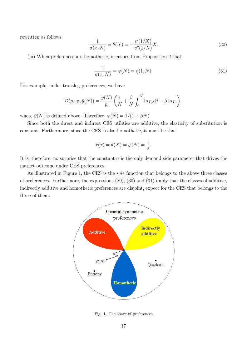
As illustrated in Figure 1, the CES is the sole function that belongs to the above three classesof preferences. Furthermore, the expressions (29), (30) and (31) imply that the classes of additive,indirectly additive and homothetic preferences are disjoint, expect for the CES that belongs to thethree of them.
Fig. 1. The space of preferences
17

By contrast, the entropy utility does not belong to any of these three classes of preferences.Indeed, it is readily verified that
�(x,N) = U
0(Nx) + lnN, (32)
which decreases with x, whereas �(x,N) is decreasing, [-shaped or increasing in N .>From now on, we consider the function �(x,N) as the primitive of the model. There are
two reasons for making this choice. First, �(x,N) portrays what preferences are along the diagonal(x
i
= x > 0 for all i). As a result, what matters for the equilibrium is how �(x,N) varies with x andN . Second, the properties of the market outcome can be characterized by necessary and sufficientconditions stated in terms of the elasticity of � with respect to x and N , which are denoted E
x
(�)
and E
N
(�). To be precise, the signs of these two expressions (Ex
(�) ? 0 and E
N
(�) 7 0) and theirrelationship (E
x
(�) ? E
N
(�)) will allow us to characterize completely the market equilibrium.How � varies with x is a priori not clear. Marshall (1920, Book 3, Chapter IV) has argued
on intuitive grounds that the elasticity of the inverse demand ⌘(x
i
,x) increases in sales.6 In oursetting, (25) shows that this assumption amounts to @�(x,x)/@x < 0. However, this inequalitydoes not tell us anything about the sign of @�(x,N)/@x because x refers here to the consumptionof all varieties. When preferences are additive, as in Krugman (1979), Marshall’s argument canbe applied because the marginal utility of a variety depends only upon its own consumption. Butthis ceases to be true when preferences are non-additive. Nevertheless, as will be seen in Section4.3, E
x
(�) < 0 holds if and only if the pass-through is smaller than 100%. The literature onspatial pricing backs up this assumption, though it also recognizes the possibility of a pass-throughexceeding 100% (Greenhut et al., 1987).
We now come to the relationship between � and N . The literature in industrial organizationsuggests that varieties become closer substitutes when N increases, the reason being that addingnew varieties crowds out the product space (Salop, 1979; Tirole, 1988). Therefore, assumingE
N
(�) > 0 spontaneously comes to mind. As a consequence, the folk wisdom would be describedby the following two conditions:
E
x
(�) < 0 < E
N
(�). (33)
However, these inequalities turn out to be more restrictive that what they might seem atfirst glance. Indeed, they do not allow us to capture some interesting market effects and fail toencompass some standard models of monopolistic competition. For example, when preferencesare quadratic, Bertoletti and Epifani (2014) have pointed out that the elasticity of substitutiondecreases with N :
�(x,N) =
↵� �x
�x
�
�
�
N. (34)
6We thank Peter Neary for having pointed out this reference to us.
18
This should not come as a surprise. Indeed, although spatial models of product differentiationand models of monopolistic competition are not orthogonal to each other, they differ in severalrespects. In particular, when consumers are endowed with a love for variety, they are inclined tospread their consumption over a wider range of varieties at the expense of their consumption ofeach variety. By contrast, in spatial models every consumer has a unique ideal variety. Therefore,providing a reconciliation of the two settings is not an easy task (Anderson et al., 1992). In whatfollows, we propose to study the impact of N on � under the assumption that a consumer’s totalconsumption Nx is arbitrarily fixed, as in spatial models of product differentiation, while allowingthe per variety consumption x to vary with N , as in love-for-variety models.
In this case, it is readily verified that the following two relationships must hold simultaneously:
dxx
= �
dNN
d��
=
@�
@N
N
�
dNN
+
@�
@x
x
�
dxx
.
Plugging the first expression into the second, we obtain
d�dN
����Nx=const
=
�
N
(E
N
(�)� E
x
(�)) .
In this event, the elasticity of substitution increases with N if and only if
E
x
(�) < E
N
(�) (35)
holds. This condition is less stringent than @�/@N > 0 because it allows the elasticity of substitu-tion to decrease with N . In other words, entry may trigger more differentiation, perhaps becausethe incumbents react by adding new attributes to their products (see, e.g., Anderson et al., 1992for an example). In addition, the evidence supporting the assumption E
x
(�) < 0 being mixed, wefind it relevant to investigate the implications of the two cases, E
x
(�) > 0 and E
x
(�) < 0. Notethat @�/@x = @�/@N = 0 in the CES case only.
4 Symmetric monopolistic competition
In the previous section, we have determined the equilibrium price, output and consumption con-ditional on the mass N of firms. Here, we pin down the equilibrium value of N by using thezero-profit condition.
A symmetric free-entry equilibrium (SFE) is described by the vector (q⇤, p⇤, x⇤, N
⇤), where N
⇤
solves the zero-profit condition⇡(N) = F, (36)
19

while q
⇤= q(N
⇤), p⇤ = p(N
⇤) and x
⇤= x(N
⇤). The Walras Law implies that the budget con-
straint N
⇤p
⇤x
⇤= y is satisfied. Without loss of generality, we restrict ourselves to the domain of
parameters for which N
⇤< N .
Combining (27) and (36), we obtain a single equilibrium condition given by
m(N) =
NF
Ly
, (37)
which means that, at the SFE, the equilibrium markup is equal to the share of the labor supplyspent on overhead costs. When preferences are non-homothetic, (22) and (24) show that L/F andy enter the function m(N) as two distinct parameters. This implies that L and y have a differentimpact on the equilibrium markup, while a hike in L is equivalent to a drop in F .
4.1 Existence and uniqueness of a SFE
Differentiating (28) with respect to N , we obtain
⇡
0(N) = x
0(N)
ddx
cLx
� (x, yL/(cLx+ F ))� 1
�����x=x(N)
= �
y
cN
2
✓� � 1� x
@�
@x
+
cLx
cLx+ F
yL
cLx+ F
@�
@N
◆����x=x(N)
.
Using (22) and (36), the second term in the right-hand side of this expression is positive if andonly if
E
x
(�) <
� � 1
�
(1 + E
N
(�)). (38)
Therefore, ⇡0(N) < 0 for all N if and only if (38) holds. This implies the following proposition.
Proposition 3. Assume (A). There exists a unique free-entry equilibrium for all c > 0 if andonly if (38) holds. Furthermore, this equilibrium is symmetric.
Because the above proposition provides a necessary and sufficient condition for the existence ofa SFE, we may safely conclude that the set of assumptions required to bring into play monopolisticcompetition must include (38). Therefore, throughout the remaining of the paper, we assume that(38) holds. This condition allows one to work with preferences that display a great of flexibility.Indeed, � may decrease or increase with x and/or N . To be precise, varieties may become betteror worse substitutes when the per variety consumption and/or the number of varieties rises, thusgenerating either price-decreasing or price-increasing competition. Evidently, (38) is satisfied whenthe folk wisdom conditions (33) hold.
Under additive preferences, (38) amounts to assuming that E
x
(�) < (� � 1)/�, which meansthat � cannot increase “too fast” with x. In this case, as shown by (37), there exists a unique SFE
20

and the markup function m(N) increases with N provided that the slope of m is smaller thanF/Ly. In other words, a market mimicking anti-competitive effects need not preclude the existenceand uniqueness of a SFE (Zhelobodko et al., 2012). When preferences are homothetic, (38) holdsif and only if E
N
(�) exceeds �1, which means that varieties cannot become too differentiated whentheir number increases, which seems reasonable.
We consider (35) and (38) as our most preferred assumptions. The former, which states thatthe impact of a change in the number of varieties on � dominates the impact of a change in theper variety consumption, points to the importance of the variety range for consumers, while thelatter is a necessary and sufficient for the existence and uniqueness of a SFE. Taken together, (35)and (38) define a range of possibilities which is broader than the one defined by (33). We willrefrain from following an encyclopedic approach in which all cases are systematically explored.However, since (35) need not hold for a SFE to exist, we will also explore what the properties ofthe equilibrium become when this condition is not met. In so doing, we are able to highlight therole played by (35) for some particular results to hold.
4.2 Comparative statics
In this subsection, we study the impact of a higher gross domestic product on the SFE. A highertotal income may stem from a larger population L, a higher per capita income y, or both. Next,we will discuss the impact of firm’s productivity. To achieve our goal, it proves to be convenientto work with the markup as the endogenous variable. Setting m ⌘ FN/(Ly), we may rewrite theequilibrium condition (37) as a function of m only:
m�
✓F
cL
1�m
m
,
Ly
F
m
◆= F. (39)
Note that (39) involves the four structural parameters of the economy: L, y, c and F . Fur-thermore, it is readily verified that the left-hand side of (39) increases with m if and only if (38)holds. Therefore, to study the impact of a specific parameter, we only have to find out how thecorresponding curve is shifted.
Before proceeding, we want to stress that we provide below a complete description of thecomparative static effects through a series of necessary and sufficient conditions. Doing this allowsus to single out what seems to be the most plausible assumptions.
4.2.1 The impact of population size
Let us first consider the impact on the market price p
⇤. Differentiating (39) with respect to L, wefind that the right-hand side of (39) is shifted upwards under an increase in L if and only if (35)holds. As a consequence, the equilibrium markup m
⇤, whence the equilibrium price p
⇤, decreaseswith L. This is in accordance with Handbury and Weinstein (2013) who observe that the price
21

level for food products falls with city size. In this case, (39) implies that the equilibrium value of� increases, which amounts to saying that varieties get less differentiated in a larger market, verymuch like in spatial models of product differentiation.
Second, the zero-profit condition implies that L always shifts p
⇤ and q
⇤ in opposite directions.Therefore, firm sizes are larger in bigger markets, as suggested by the empirical evidence providedby Manning (2010).
How does N
⇤ change with L? Differentiating (28) with respect to L, we have
@⇡
@L
����N=N
⇤=
cx
� (x,N)� 1
+
@x(N)
@L
@
@x
✓cLx
� (x,N)� 1
◆����x=x
⇤,N=N
⇤. (40)
Substituting F for ⇡(N⇤) and simplifying, we obtain
@⇡
@L
����N=N
⇤=
cx�
(� � 1)
3
(� � 1� E
x
(�))
�����x=x
⇤,N=N
⇤.
Since the first term in the right-hand side of this expression is positive, (40) is positive if and onlyif the following condition holds:
E
x
(�) < � � 1. (41)
In this case, a population growth triggers the entry of new firms. Furthermore, restating (37)as N/m(N) = Ly/F , it is readily verified that the increase in N
⇤is less proportional than thepopulation hike if and only if m0
(N) < 0, which is equivalent to (35).Observe that (38) implies (41) when preferences are (indirectly) additive, while (41) holds true
under homothetic preferences because E
x
(�) = 0.It remains to determine how the per variety consumption level x⇤ varies with an increase in
population size. Combining (24) with the budget constraint x = y/(pN), we obtain
Nx�(x,N)
�(x,N)� 1
=
y
c
. (42)
Note that L does not enter (42) as an independent parameter. Furthermore, it is straightforwardto check that the left-hand side of (42) increases with x when (41) holds, and decreases otherwise.Combining this with the fact that (41) is also necessary and sufficient for an increase in L to triggeradditional entry, the per variety consumption level x⇤ decreases with L if and only if the left-handside of (42) increases with N , or, equivalently, if and only if
E
N
(�) < � � 1. (43)
This condition holds if � decreases with N or increases with N , but not “too fast,” which meansthat varieties do not get too differentiated with the entry of new firms. Note also that (35) and(43) imply (41). Evidently, (43) holds for (i) additive preferences, for in this case E
N
(�) = 0, while
22

� > 1; (ii) indirectly additive preferences, because, using (41) and �(x,N) = 1/✓(xN), we obtain1 + E
N
(�) = 1 + E
x
(�) < �; and (iii) any preferences such that � weakly decreases with N .The following proposition comprises a summary.Proposition 4. If E
x
(�) is smaller than E
N
(�), then a higher population size results in alower markup and larger firms. Furthermore, if (43) holds, the mass of varieties increases lessthan proportionally with L, while the per variety consumption decreases with L.
Note that the mass of varieties need not rise with the population size. Indeed, N⇤ falls whenE
N
(�) exceeds �� 1. In this case, increasing the number of firms makes varieties very close substi-tutes, which strongly intensifies competition among firms. Under such circumstances, the benefitsassociated with diversity are low, thus implying that consumers value more and more the volumesthey consume. This in turn leads a fraction of incumbents to get out of business.
When preferences are homothetic, � depends upon N only. In this case, (42) boils down to
1 +
N'
0(N)
1� '(N)
> 0.
When '
0(N) < 0, this inequality need not hold. However, in the case of the translog where
'(N) = 1/(1 + �N), (42) is satisfied, and thus x
⇤ decreases with L.What happens when E
x
(�) > E
N
(�)? In this event, (38) implies that (43) holds. Therefore,the above necessary and sufficient conditions imply the following result: If E
x
(�) < E
N
(�), thena higher population size results in a higher markup, smaller firms, a more than proportional risein the mass of varieties, and a lower per variety consumption. As a consequence, a larger marketmay generate anti-competitive effects that take the concrete form of a higher market price and lessefficient firms producing at a higher average cost. Such results are at odds with the main body ofindustrial organization, which explains why (35) is one of our most preferred conditions.
4.2.2 The impact of individual income
We now come to the impact of the per capita income on the SFE. One expects a positive shockon y to trigger the entry of new firms because more labor is available for production. However,consumers have a higher willingness-to-pay for the incumbent varieties and can afford to buy eachof them in a larger volume. Therefore, the impact of y on the SFE is a priori ambiguous.
Differentiating (39) with respect to y, we see that the left-hand side of (39) is shifted downwardsby an increase in y if and only if E
N
(�) > 0. In this event, the equilibrium markup decreases withy.
To check the impact of y on N
⇤, we differentiate (28) with respect to y and get
@⇡(N)
@y
����N=N
⇤=
@x(N)
@y
@
@x
✓cLx
� (x,N)� 1
◆�����x=x
⇤,N=N
⇤.
After simplification, this yields
23

@⇡(N)
@y
����N=N
⇤=
L
N
� � 1� �E
x
(�)
(� � 1)
2
����x=x
⇤,N=N
⇤.
Hence, @⇡(N⇤)/@y > 0 if and only if the following condition holds:
E
x
(�) <
� � 1
�
. (44)
Note that this condition is more stringent than (41). Thus, if EN
(�) > 0, then (44) implies (38).As a consequence, we have:Proposition 5. If E
N
(�) > 0, then a higher per capita income results in a lower markup andbigger firms. Furthermore, the mass of varieties increases with y if (44) holds, but decreases withy otherwise.
Thus, when entry renders varieties less differentiated, the mass of varieties need not rise withincome. Indeed, the increase in per variety consumption may be too high for all the incumbentsto stay in business. The reason for this is that the decline in prices is sufficiently strong for fewerfirms to operate at a larger scale. As a consequence, a richer economy need not exhibit a widerarray of varieties.
Evidently, if EN
(�) < 0, the markup is higher and firms are smaller when the income y rises.Furthermore, (38) implies (44) so that N
⇤ increases with y. Indeed, since varieties get moredifferentiated when entry arises, firms exploit consumers’ higher willingness-to-pay to sell less ata higher price, which goes together with a larger mass of varieties.
Propositions 4 and 5 show that an increase in L is not a substitute for an increase in y and viceversa, except, as shown below, in the case of homothetic preferences. This should not come as asurprise because an increase in income affects the shape of individual demands when preferencesare non-homothetic, whereas an increase in L shifts upward the market demand without changingits shape.
Finally, observe that using (indirectly) additive utilities allows capturing the effects generatedby shocks on population size (income), but disregard the impact of the other magnitude. Ifpreferences are homothetic, it is well known that the effects of L and y on the market variables p⇤,q
⇤ and N
⇤ are exactly the same. Indeed, m does not involve y as a parameter because � dependssolely on N . Therefore, it ensues from (37) that the equilibrium price, firm size, and number offirms depend only upon the total income yL.
4.2.3 The impact of firm productivity
Firms’ productivity is typically measured by their marginal costs. To uncover the impact on themarket outcome of a productivity shock common to all firms, we conduct a comparative staticanalysis of the SFE with respect to c and show that the nature of preferences determines theextent of the pass-through. In particular, we establish that the pass-through rate is lower than
24

100% if and only if � decreases with x, i.e.
E
x
(�) < 0 (45)
holds. Evidently, the pass-through rate exceeds 100% when 0 < E
x
(�).Figure 2 depicts (37). It is then straightforward to check that, when � decreases with x, a drop
in c moves the vertical line rightward, while the p
⇤-locus is shifted downward. As a consequence,the market price p
⇤ decreases with c. But by how much does p
⇤ decrease relative to c?
E
x
(�) < 0 E
x
(�) > 0
Fig. 2. Productivity and entry.
The left-hand side of (39) is shifted downwards under a decrease in c if and only if Ex
(�) < 0.In this case, both the equilibrium markup m
⇤ and the equilibrium mass of firms N⇤= (yL/F ) ·m
⇤
increases with c. In other words, when E
x
(�) < 0, the pass-through rate is smaller than 1 becausevarieties becomes more differentiated, which relaxes competition. On the contrary, when E
x
(�) > 0,the markup and the mass of firms decrease because varieties get less differentiated. In other words,competition becomes so tough that p
⇤ decreases more than proportionally with c. In this event,the pass-through rate exceeds 1.
Under homothetic preferences, (Ex
(�) = 0), p(N) is given by
p(N) =
c
1� '(N)
=) m(N) = '(N).
As a consequence, (37) does not involve c as a parameter. This implies that a technological shockdoes affect the number of firms. In other words, the markup remains the same regardless of theproductivity shocks, thereby implying that under homothetic preferences the pass-through rateequal to 1.
The impact of technological shocks on firms’ size leads to ambiguous conclusions. For example,under quadratic preferences, q⇤ may increase and, then, decreases in response to a steadily dropin c.
25

The following proposition comprises a summary.Proposition 6. If the marginal cost of firms decreases, (i) the market price decreases and (ii)
the markup and number of firms increase if and only if (45) holds.This proposition has an important implication. If the data suggest a pass-through rate smaller
than 1, then it must be that E
x
(�) < 0. In this case, (41) must hold while (38) is satisfied whenE
N
(�) exceeds �1, thereby a bigger or richer economy is more competitive and more diversifiedthan a smaller or poorer one. Note that (38) does not restrict the domain of admissible valuesof E
x
(�) for a pass-through rate to be smaller than 1, whereas (38) requires that E
x
(�) cannotexceed (1 � 1/�) (1 + E
N
(�)). Recent empirical evidence shows that the pass-through generatedby a commodity tax or by trade costs need not be smaller than 1 (Martin, 2012, and Weyl andFabinger, 2013). Our theoretical argument thus concurs with the inconclusive empirical evidence:the pass-through rate may exceed 1, although it is more likely to be less than 1.
Let us make a pause and summarize what our main results are. We have found necessary andsufficient conditions for the existence and uniqueness of a SFE (Proposition 3), and provided acomplete characterization of the effect of a market size or productivity shock (Propositions 4 to6). Observing that (33) implies (38), (35) and (44), we may conclude that a unique SFE exists(Proposition 3), that a larger market or a higher income leads to lower markups, bigger firms anda larger number of varieties (Propositions 4 and 5), and that the pass-through rate is smaller than1 (Proposition 6) if (33) holds. Recall, however, that less stringent conditions are available foreach of the above-mentioned properties to be satisfied separately.
4.2.4 Monopolistic versus oligopolistic competition
It should be clear that Propositions 4-6 have the same nature as results obtained in similar compar-ative analyses conducted in oligopoly theory (Vives, 1999). They may also replicate less standardanti-competitive effects under some specific conditions (Chen and Riordan, 2008).
The markup (27) stems directly from preferences through the sole elasticity of substitution be-cause we focus on monopolistic competition. However, in symmetric oligopoly models the markupemerges as the outcome of the interplay between preferences and strategic interactions. Neverthe-less, at least to a certain extent, both settings can be reconciled.
To illustrate, consider the case of an integer number N of quantity-setting firms and of anarbitrary utility U(x
1
, ..., x
N
). The inverse demands are given by
p
i
=
U
i
�
� =
1
y
NX
j=1
x
j
U
j
.
Firm i’s profit-maximization condition is given by
26
p
i
� c
p
i
= �
x
i
U
ii
U
i
+ E
xi(�) = �
x
i
U
ii
U
i
+
x
i
U
i
+
PN
j=1
x
i
x
j
U
ij
PN
j=1
x
j
U
j
. (46)
Set
r
o
(x,N) ⌘ �
xU
ii
(x, ..., x)
U
i
(x, ..., x)
r
c
(x,N) ⌘
xU
ij
(x, ..., x)
U
i
(x, ..., x)
for j 6= i.
The symmetry of preferences implies that ro
(x,N) and r
c
(x,N) are independent of i and j.Combining (46) with the symmetry condition x
i
= x, we obtain the markup condition:
p� c
p
=
1
N
+
✓1�
1
N
◆[r
o
(x,N) + r
c
(x,N)] . (47)
The elasticity of substitution s
ij
between varieties i and j is given by (see Appendix 4)
s
ij
= �
U
i
U
j
(x
i
U
j
+ x
j
U
i
)
x
i
x
j
⇥U
ii
U
2
j
� 2U
ij
U
i
U
j
+ U
jj
U
2
i
⇤. (48)
When the consumption pattern is symmetric, (48) boils down to
s(x,N) =
1
r
o
(x,N) + r
c
(x,N)
. (49)
Combining (47) with (49), we get
p� c
p
=
1
N
+
✓1�
1
N
◆1
s(x,N)
. (50)
Unlike the profit-maximization condition (50), product and labor market balance, as well asthe zero-profit condition, do not depend on strategic considerations. Since
p� c
p
=
1
�(x,N)
(51)
under monopolistic competition, comparing (51) with (50) shows that the set of Cournot symmetricfree-entry equilibria is the same as the set of equilibria obtained under monopolistic competition ifand only if �(x,N) is given by
1
�(x,N)
=
1
N
+
✓1�
1
N
◆1
s(x,N)
.
As a consequence, by choosing appropriately the elasticity of substitution as a function of xand N , monopolistic competition is able to replicate not only the direction of comparative staticeffects generated in symmetric oligopoly models with free entry, but also their magnitude. Hence,we find it to say that monopolistic competition under non-separable preferences mimics oligopolisticcompetition.
27

4.3 When is the SFE socially optimal?
The social planner faces the following optimization problem:
maxU(x) s.t. Ly = cL
ˆN
0
x
i
di+NF.
The first-order condition with respect to x
i
implies that the problem may be treated usingsymmetry, so that the above problem may be reformulated as maximizing
�(x,N) ⌘ U
�xI
[0,N ]
�
subject to Ly = N(cLx+ F ).The ratio of the first-order conditions with respect to x and N leads to
�
x
�
N
=
NcL
cLx+ F
. (52)
It is well known that the comparison of the social optimum and market outcome leads toambiguous conclusions for the reasons provided by Spence (1976). We illustrate here this difficultyin the special case of homothetic preferences. Without loss of generality, we can write �(N, x) asfollows:
�(N, x) = N (N)x,
where (N) is an increasing function of N . In this event, we get �x
x/� = 1 and �
N
N/� =
1 +N
0/ . Therefore, (52) becomes
E
N
( ) =
F
cLx
,
while the market equilibrium condition (37) is given by
'(N)
1� '(N)
=
F
cLx
.
The social optimum and the market equilibrium are identical if and only if
E
N
( ) =
'(N)
1� '(N)
. (53)
It should be clear that this condition is unlikely to be satisfied unless strong restrictions areimposed on the utility. To be concrete, denote by A(N) the solution to
E
N
(A) + E
N
( ) =
'(N)
1� '(N)
,
which is unique up to a positive coefficient. It is then readily verified that (53) holds for all N if and
28

only if �(x,N) is replaced with A(N)�(x,N). Thus, contrary to the folk wisdom, the equilibriumand the optimum may be the same for utility functions that differ from the CES (Dhingra andMorrow, 2013). This finding has an unexpected implication.
Proposition 7. If preferences are homothetic, there exists a consumption externality for whichthe equilibrium and the optimum coincide regardless of the values taken by the parameters of theeconomy.
Hence, the choice of a particular consumption externality has subtle welfare implications, whichare often disregarded in the literature. For example, if we multiply A(N) by N
⌫ , where ⌫ is aconstant, there is growing under-provision of varieties when the difference ⌫� 1/(� � 1) < 0 falls,and growing over-provision when ⌫� 1/(� � 1) > 0 rises. This has the following unsuspectedimplication: preferences given by A(N)�(x,N) are cardinal in nature. Indeed, taking a powertransformation of N
⌫
�(x,N) makes the discrepancy between the equilibrium and the optimumcan be made arbitrarily large or small by choosing the appropriate value of the exponent ⌫.
5 Extensions
In this section, we extend our baseline model to heterogeneous firms. We then consider the caseof a multisector economy and conclude with a discussion of a setting in which consumers areheterogeneous.
5.1 Heterogeneous firms
It is natural to ask whether the approach developed in this paper can cope with Melitz-like het-erogeneous firms? In what follows, we consider the one-period framework used by Melitz andOttaviano (2008), the mass of potential firms being given by N . Prior to entry, risk-neutral firmsface uncertainty about their marginal cost while entry requires a sunk cost F
e
. Once this cost ispaid, firms observe their marginal cost drawn randomly from the continuous probability distri-bution �(c) defined over R
+
. After observing its type c, each entrant decides to produce or not,given that an active firm must incur a fixed production cost F . Under such circumstances, themass of entrants, N
e
, typically exceeds the mass of operating firms, N . Even though varieties aredifferentiated from the consumer’s point of view, firms sharing the same marginal cost c behavein the same way and earn the same profit at equilibrium. As a consequence, we may refer to anyvariety/firm by its c-type only.
The equilibrium conditions are as follows:(i) the profit-maximization condition for c-type firms:
max
xc
⇧
c
(x
c
,x) ⌘
D (x
c
,x)
�
� c
�Lx
c
� F ; (54)
29

(ii) the zero-profit condition for the cutoff firm:
(p
c
� c)q
c
= F,
where c is the cutoff cost. As will be shown below, firms are sorted out by decreasing order ofproductivity, which implies that the mass of active firms is equal to N ⌘ N
e
�(c);(iii) the product market clearing condition:
q
c
= Lx
c
for all c 2 [0, c];(iv) the labor market clearing condition:
N
e
F
e
+
ˆc
0
(cq
c
+ F )d�(c)�= yL,
where N
e
is the number of entrants;(v) firms enter the market until their expected profits net of the entry cost F
e
are zero:
ˆc
0
⇧
c
(x
c
,x)d�(c) = F
e
. (55)
When c
i
> c
j
, (54) impliesD (x
ci ,x)
�
� c
i
�Lx
i
<
D (x
ci ,x)
�
� c
j
�Lx
ci ,
so that there is perfect sorting across firms’ types at any equilibrium, while firms with a higherproductivity earn higher profits.
It also follows from (54) that p
c
[1� ⌘(x
c
,x)] = c. Combining this with the inverse demandsyields
D(x
c
,x) [1� ⌘(x
c
,x)] = �c. (56)
Dividing (56) for a type-ci
firm by the same expression for a type-cj
firm, we obtain
D(x
ci ,x) [1� ⌘(x
ci ,x)]
D(x
cj ,x)
⇥1� ⌘(x
cj ,x)
⇤=
c
i
c
j
. (57)
The condition (A) of Section 3 means that, for any given x, a firm’s marginal revenue D(x,x) [1� ⌘(x,x)]
decreases with x. Therefore, it ensues from (57) that xi
> x
j
if and only if ci
< c
j
. In other words,more efficient firms produce more than less efficient firms. Furthermore, since p
i
= D(x,x)/� andD decreases in x for any given x, more efficient firms sell at lower prices than less efficient firms.As for the markups, (57) yields
30

p
i
/c
i
p
j
/c
j
=
1� ⌘(x
cj ,x)
1� ⌘(x
ci ,x)
.
Consequently, more efficient firms enjoy higher markups – a regularity observed in the data (DeLoecker and Warzynski, 2012) – if and only if ⌘(x,x) increases with x, i.e., (Abis) holds (seeSection 3.1).
The following proposition is a summary.Proposition 8. Assume that firms are heterogeneous. If (A) holds, then more efficient firms
produce larger outputs, charge lower prices and earn higher profits than less efficient firms. Fur-thermore, more efficient firms have higher markups if (Abis) holds, but lower markups otherwise.
From now on, we assume that, for any c and N
e
, there exists a unique equilibrium ¯
x(c, N
e
) ofthe quantity game. Since the distribution G is given, the profit-maximization condition impliesthat x⇤ is entirely determined by c and N
e
. In other words, regardless of the nature of preferencesand the distribution of marginal costs, the heterogeneity of firms amounts to replacing the variableN by the two variables c and N
e
. As for x, it is replaced by c because the c-type firms sell at aprice that depends on c, thus making c-specific the consumption of the corresponding varieties. Asa consequence, the complexity of the problem goes from two to three dimensions. The equilibriumoperating profits of the quantity game may thus be written as follows:
⇧
⇤c
(c, N
e
) ⌘ max
xc
D (x
c
,x
⇤(c, N
e
))
� (x
⇤(c, N
e
))
� c
�Lx
c
.
We have seen that ⇧
⇤c
(c, N
e
) decreases with c. In what follows, we impose the additional twoconditions that rule out anti-competitive market outcomes.
(B) The equilibrium profit of each firm’s type decreases in c and N
e
.The intuition behind this assumption is easy to grasp: a larger number of entrants or a higher
cutoff leads to lower profits, for, in both cases, the mass of active firms N rises. To illustrate,consider first the case of CES preferences where the equilibrium profits are given by
⇧
⇤c
(c, N
e
) =
yL
�N
e
c
1��´c
0
z
1��dG(z)
, (58)
which implies (B). More generally, using Zhelobodko et al. (2012), it is readily verified that anyadditive preference satisfies (B). The same holds for indirectly additive preferences. To see this,observe that (58) boils down to
⇧
⇤c
(c, N
e
) =
yL
N
e
v
0(p(c, y)/y) [p(c, y)� c]´
c
0
v
0(p(z, y)/y)p(c, y)dG(z)
, (59)
where p(c, y) is the c-type firm profit-maximizing price solving the first-order condition p(1 �
✓(y/p)) = c. Clearly, (B) follows from (59).In what follows, we assume that, for any c and N
e
, there exists a unique equilibrium ¯
x(c, N
e
)
31

of the quantity game and allow for the endogenous determination of c and N
e
.
Free-entry equilibria. A free-entry equilibrium with heterogeneous firms is defined by a pair(c
⇤, N
⇤e
) that satisfies the zero-expected-profit condition for each firmˆ
c
0
[⇧
⇤c
(c, N
e
)� F ] d�(c) = F
e
, (60)
as well as the cutoff condition
⇧
⇤c
(c, N
e
) = F. (61)
Dividing (60) by (61) yields the following new equilibrium condition:
ˆc
0
⇧
⇤c
(c, N
e
)
⇧
⇤c
(c, N
e
)
� 1
�d�(c) =
F
e
F
. (62)
Let c = g(N
e
) be the locus of solutions to (61) and c = h(N
e
) the locus of solutions to (62).7 Afree-entry equilibrium is thus an intersection point of the two loci c = g(N
e
) and c = h(N
e
) in the(N
e
, c)-plane. As implied by (B), g(Ne
) is downward-sloping in the (N
e
, c)-plane. Furthermore,it is shifted upward when L rises. As for h(N
e
), it is independent of L but its slope is a prioriundetermined. Yet, we will see that the sign of the slope of h(N
e
) is critical for the impact of apopulation hike on the cutoff cost.
Three cases may arise. First, if the locus h(N
e
) is upward-sloping, there exists a unique free-entry equilibrium, and this equilibrium is stable. Furthermore, both N
⇤e
and c
⇤ increase with L
(see Figure 3a). Let us now rotate the locus h(N
e
) in a clockwise manner, so that h(N
e
) gets lessand less steep. The second case, which corresponds to the CES preferences, arises when h(N
e
) ishorizontal, which implies that N
⇤e
rises with L while c
⇤ remains constant.
Fig. 3a. Cutoff and market size
7We give below sufficient conditions for the left-hand side of (62) to be monotone in c and Ne, two conditionsthat garantee that the locus c = h(Ne) is well defined.
32
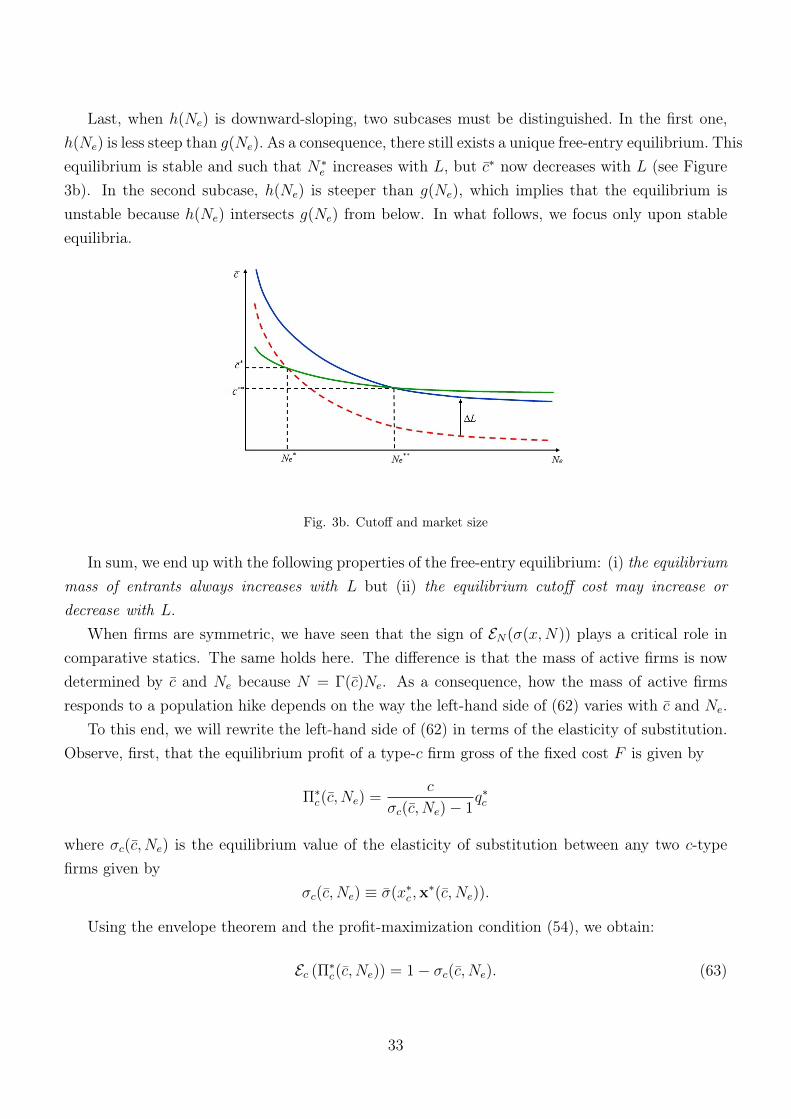
Last, when h(N
e
) is downward-sloping, two subcases must be distinguished. In the first one,h(N
e
) is less steep than g(N
e
). As a consequence, there still exists a unique free-entry equilibrium. Thisequilibrium is stable and such that N
⇤e
increases with L, but c
⇤ now decreases with L (see Figure3b). In the second subcase, h(N
e
) is steeper than g(N
e
), which implies that the equilibrium isunstable because h(N
e
) intersects g(N
e
) from below. In what follows, we focus only upon stableequilibria.
Fig. 3b. Cutoff and market size
In sum, we end up with the following properties of the free-entry equilibrium: (i) the equilibriummass of entrants always increases with L but (ii) the equilibrium cutoff cost may increase ordecrease with L.
When firms are symmetric, we have seen that the sign of EN
(�(x,N)) plays a critical role incomparative statics. The same holds here. The difference is that the mass of active firms is nowdetermined by c and N
e
because N = �(c)N
e
. As a consequence, how the mass of active firmsresponds to a population hike depends on the way the left-hand side of (62) varies with c and N
e
.To this end, we will rewrite the left-hand side of (62) in terms of the elasticity of substitution.
Observe, first, that the equilibrium profit of a type-c firm gross of the fixed cost F is given by
⇧
⇤c
(c, N
e
) =
c
�
c
(c, N
e
)� 1
q
⇤c
where �c
(c, N
e
) is the equilibrium value of the elasticity of substitution between any two c-typefirms given by
�
c
(c, N
e
) ⌘ �(x
⇤c
,x
⇤(c, N
e
)).
Using the envelope theorem and the profit-maximization condition (54), we obtain:
E
c
(⇧
⇤c
(c, N
e
)) = 1� �
c
(c, N
e
). (63)
33
Since
�
ˆc
c
E
z
(⇧
⇤z
(c, N
e
))
z
dz = �
ˆc
c
@ ln⇧
⇤z
(c, N
e
)
@z
dz = ln⇧
⇤c
(c, N
e
)� ln⇧
⇤c
(c, N
e
),
it follows from (63) that
ln⇧
⇤c
(c, N
e
)
ln⇧
⇤c
(c, N
e
)
=
ˆc
c
�
z
(c, N
e
)� 1
z
dz.
Accordingly, (62) may rewritten as follows:ˆ
c
0
exp
✓ˆc
c
�
z
(c, N
e
)� 1
z
dz
◆� 1
�d�(c) =
F
e
F
. (64)
Therefore, if �c
(c, N
e
) increases with c, the left-hand side of (62) increases with c. Intuitively,when c increases, the mass of firms rises as less efficient firms stay in business, which intensifiescompetition and lowers markups. In this case, the selection process is tougher. This is not the endof the story, however. Indeed, the competitiveness of the market also depends on how N
e
affectsthe degree of differentiation across varieties.
The expression (64) shows that the left-hand side of (62) increases with N
e
if and only if�
c
(c, N
e
) increases in N
e
. This amounts to assuming that, for any given cutoff, the relative impactof entry on the low-productivity firms (i.e., the small firms) is larger than the impact on the high-productivity firms, the reason being that E
c
(⇧
⇤c
(c, N
e
)) decreases in N
e
if and only if �c
(c, N
e
)
increases in N
e
.When �
c
(c, N
e
) increases both with c and N
e
, the locus h(N
e
) is downward-sloping. Indeed,when N
e
rises, so does the left-hand side of (64). Hence, since �c
(c, N
e
) also increases with c, itmust be that c decreases for (64) to hold. As a consequence, we have:
Claim 1. Assume (B). If �c
(c, N
e
) increases with c and N
e
, then c
⇤ decreases with L.Given c, the number of active firms N is proportional to the number of entrants N
e
. Therefore,assuming that �(c, N
e
) increases with N
e
may be considered as the counterpart of one of our mostpreferred assumptions in the case of symmetric firms, that is, �(x,N) increases with N . In thiscase, the pro-competitive effect generated by entry exacerbates the selection effect across firms.In response to a hike in L, the two effects combine to induce the exit of the least efficient activefirms. This echoes Melitz and Ottaviano (2008) who show that a trade liberalization shock givesrise to a similar effect under quadratic preferences. Since N
⇤e
and c
⇤ move in opposite directions,it is hard to predict how L affects the equilibrium mass N⇤ of active firms. Indeed, how strong arethe entry and selection effects depends on the elasticity of substitution and the distribution G.
Repeating the above argument shows that, when �c
(c, N
e
) increases with c and decreases withN
e
, the locus h(N
e
) is upward-sloping. In this event, we have:Claim 2. Assume (B). If �
c
(c, N
e
) increases with c and decreases with N
e
, then c
⇤ increaseswith L.
34
When �c
(c, N
e
) decreases with N
e
, two opposing effects are at work. First, entry fosters productdifferentiation, and thus relaxes competition. This invites new firms to enter and allows less efficientfirms to stay in business. On the other hand, the corresponding hike in c tends to render varietiescloser substitutes. What our result shows is that the former effect dominates the latter. Hence,the equilibrium mass of active firms N
⇤= �(c
⇤)N
⇤e
unambiguously rises with L.To conclude, the impact of population size on the number of entrants is unambiguous: a larger
market invites more entry. By contrast, the cutoff cost behavior depends on how the elasticity ofsubstitution varies with N
e
. All if this shows that the interaction between the entry and selectioneffects is non-trivial.8
Finally, by reformulating the game with price-setting firms, the same comparative statics anal-ysis can be undertaken to study how the per capita income affects the market outcome.
Pass-through. We show here that the result on complete pass-through under homothetic pref-erences still holds when firms are heterogeneous. The first-order condition for a c-type firm is givenby
p
c
� c
p
c
= ⌘(x
c
,x). (65)
Consider a proportionate drop in marginal costs by a factor µ > 1, so that the distributionof marginal costs is given by G(µc). We first investigating the impact of µ on firms’ operatingprofits when the cutoff c is unchanged. The cutoff firms now have a marginal cost equal to c/µ.Furthermore, under homothetic preferences, ⌘(x
c
,x) does not depend on the income y and ispositive homogeneous of degree 0. Therefore, (65) is invariant to the same proportionate reductionin c. As a consequence, the new price equilibrium profile over [0, c] is obtained by dividing allprices by µ.
We now show that the profits of the c-type firms do not change in response to the drop incost, so that the new cutoff is given by c/µ. Indeed, both marginal costs and prices are dividedby µ, while homothetic preferences imply that demands are shifted upwards by the same factor µ.Therefore, the operating profit of the c-type firms is unchanged because
✓p
c
µ
�
c
µ
◆Lµx
c
= (p
c
� c)Lx
c
= F.
In sum, regardless of the cost distribution, under homothetic preferences the equilibrium pricedistribution changes in proportion with the cost distribution, thereby leaving unchanged the distri-bution of equilibrium markups, as in Proposition 6.
8Note that we do not say anything about the impact on the aggregate productivity. This one will depend uponthe aggregation weights chosen, as well on the distribution of firms’ types, which is here unspecified.
35

5.2 Multisector economy
Following Dixit and Stiglitz (1977), we consider a two-sector economy involving a differentiatedgood supplied under increasing returns and monopolistic competition, and a homogeneous good- or a Hicksian composite good - supplied under constant returns and perfect competition. Bothgoods are normal. Labor is the only production factor and is perfectly mobile between sectors.Consumers share the same preferences given by U(U(x), x
0
) where the functional U (x) satisfiesthe properties stated in Section 2, while x
0
is the consumption of the homogeneous good. Theupper-tier utility U is strictly quasi-concave, once continuously differentiable, strictly increasingin each argument, and such that the demand for the differentiated product is always positive.9
Choosing the unit of the homogeneous good for the marginal productivity of labor to be equalto 1, the equilibrium price of the homogeneous good is equal to 1. Since profits are zero at theSFE, the budget constraint is given by
ˆN
0
p
i
x
i
di+ x
0
= E + x
0
= y, (66)
where the expenditure E on the differentiated good is endogenous because competition across firmsaffects the relative price of this good.
Using the first-order condition for utility maximization yields
p
i
=
U
01
(U (x), x
0
)
U
02
(U (x), x
0
)
D(x
i
, x).
Let p be arbitrarily given. Along the diagonal xi
= x, this condition becomes
p = S(�(x,N), x
0
)D(x, xI
[0,N ]
), (67)
where S is the marginal rate of substitution between the differentiated and homogeneous goods:
S(�, x
0
) ⌘
U
01
(�(x,N), x
0
)
U
02
(�(x,N), x
0
)
and �(x,N) ⌘ U
�xI
[0,N ]
�.
The quasi-concavity of the upper-tier utility U implies that the marginal rate of substitutiondecreases with �(x,N) and increases with x
0
. Therefore, for any given (p, x,N), (67) has a uniquesolution x
0
(p, x,N), which is the income-consumption curve. The two goods being normal, thiscurve is upward sloping in the plane (x, x
0
).For any given x
i
= x, the love for variety implies that the utility level increases with the numberof varieties. However, it is reasonable to suppose that the marginal utility D of an additional varietydecreases. To be precise, we assume that
9Our results hold true if the choke price is finite but sufficiently high.
36
(C) for all x > 0, the marginal utility D weakly decreases with the number of varieties.Observe that (C) holds for additive and quadratic preferences. Since �(x,N) increases in N ,
S decreases. As D weakly decreases in N , it must be that x
0
increases for the condition (67) tobe satisfied. In other words, x
0
(p, x,N) increases in N .We now determine the relationship between x and m by using the zero-profit condition. Since
by definition m ⌘ (p� c)/p, for any given p the zero-profit and product market clearing conditionsyield the per variety consumption as a function of m only:
x =
F
cL
1�m
m
. (68)
Plugging (68) and p = c/(1�m) into x
0
, we may rewrite x
0
(p, x,N) as a function of m and N
only:
x
0
(m,N) ⌘ x
0
✓c
1�m
,
F
cL
1�m
m
, N
◆.
Plugging (68) and p = c/(1�m) into the budget constraint (66) and solving for N , we obtainthe income y such that the consumer chooses the quantity x
0
(m,N) of the homogeneous good:
N =
Lm
F
[y � x
0
(m,N)] . (69)
Since x
0
and x
0
vary with N identically, x
0
also increases in N . Therefore, (69) has a uniquesolution ˆ
N(m) for any m 2 [0, 1].Moreover, (69) implies that @ ˆ
N/@y > 0, while @ ˆ
N/@L > 0 because the income-consumptioncurve is upward slopping. In other words, if the price of the differentiated product is exogenouslygiven, an increase in population size or individual income leads to a wider range of varieties.
Since ˆ
N(m) is the number of varieties in the two-sector economy, the equilibrium condition(39) must be replaced with the following expression:
m�
✓F
cL
1�m
m
,
ˆ
N(m)
◆= 1. (70)
The left-hand side m� of (70) equals zero for m = 0 and exceeds 1 when m = 1. Hence,by the intermediate value theorem, the set of SFEs is non-empty. Moreover, it has an infimumand a supremum, which are both SFEs because the left-hand side of (70) is continuous. In whatfollows, we denote the corresponding markups by m
inf
and m
sup
; if the SFE is unique, minf
= m
sup
.Therefore, the left-hand side of (70) must increase with m in some neighborhood of m
inf
, forotherwise there would be an equilibrium to the left of m
inf
, a contradiction. Similarly, the left-hand side of (70) increases with m in some neighborhood of m
sup
.Since @ ˆ
N/@y > 0, (70) implies that an increase in y shifts the locus m� upward if and onlyif E
N
(�) > 0, so that the equilibrium markups m
inf
and m
sup
decrease in y. Consider now anincrease in population size. Since @ ˆ
N/@L > 0, (70) implies that an increase in L shifts the locus
37
m� upward if both E
x
(�) < 0 and E
N
(�) > 0 hold. In this event, the equilibrium markups m
inf
and m
sup
decrease in L.Summarizing our results, we come to a proposition.Proposition 9. Assume (C). Then, the set of SFEs is non-empty. Furthermore, (i) an increase
in individual income leads to a lower markup and bigger firms at the infimum and supremum SFEsif and only if E
N
(�) > 0 and (ii) an increase in population size yields a lower markup and biggerfirms at the infimum and supremum SFEs if E
x
(�) < 0 and E
N
(�) > 0.This extends to a two-sector economy what Propositions 4 and 5 state in the case of a one-
sector economy where the SFE is unique. Proposition 8 also shows that the elasticity of substitutionkeeps its relevance for studying monopolistic competition in a multisector economy. In contrast,studying how N
⇤ changes with L or y is more problematic because the equilibrium number ofvarieties depends on the elasticity of substitution between the differentiated and homogeneousgoods.
5.3 Heterogeneous consumers
Accounting for consumer heterogeneity in models of monopolistic competition is not easy butdoable. Let D(p
i
,p; y, ✓) be the Marshallian demand for variety i of a (y, ✓)-type consumer where✓ is the taste parameter. The aggregate demand faced by firm i is then given by
�(p
i
,p) ⌘ L
ˆR+⇥⇥
D(p
i
,p; y, ✓)dG(y, ✓), (71)
where G is a continuous joint probability distribution of income y and taste ✓.Ever since the Sonnenschein-Mantel-Debreu theorem (Mas-Colell et al., 1995, ch.17), it is well
known that the aggregate demand (71) need not inherit the properties of the individual demandfunctions. By contrast, as in Section 2, for each variety i, the aggregate demand �(p
i
,p) for varietyi is decreasing in p
i
regardless of the income-taste distribution G. A comparison with Hildenbrand(1983) and Grandmont (1987), who derived specific conditions for the Law of demand to holdwhen the number of goods is finite, shows how working with a continuum of goods, which neednot be the varieties of a differentiated product, vastly simplifies the analysis.
The properties of D crucially depend on the relationship between income and taste. Indeed,since firm i’s profit is given by ⇡(p
i
,p) = (p
i
� c)�(p
i
,p) � F , the first-order condition for asymmetric equilibrium becomes
p
1�
1
"(p,N)
�= c, (72)
where "(p,N) is the elasticity of �(p,p) evaluated at the symmetric outcome. If "(p,N) is anincreasing function of p and N , most of the results derived above hold true. Indeed, integratingconsumers’ budget constraints across R
+
⇥ ⇥ and applying the zero-profit condition yields the
38
markup.
m(N) =
NF
LY
where Y ⌘
ˆR+⇥⇥
ydG(y, ✓). (73)
Note that (73) differs from (37) only in one respect: the individual income y is replaced withthe mean income Y , which is independent of L. Consequently, if "(p,N) decreases both with p
and N , a population hike or a productivity shock affects the SFE as in the baseline model (seePropositions 4 and 6). By contrast, the impact of an increase in Y is ambiguous because it dependson how ✓ and y are related.
There is no reason to expect the aggregate demand to exhibit an increasing price elasticityeven when the individual demands satisfy this property. To highlight the nature of this difficulty,we show in Appendix 6 that
@"(p,N)
@p
=
´R+⇥⇥
@"(p,N ; y,✓)
@p
s(p,N ; y, ✓)dG(y, ✓)�
�
1
p
´R+⇥⇥
["(p,N ; y, ✓)� "(p,N)]
2
s(p,N ; y, ✓)dG(y, ✓),
(74)
where "(p,N ; y, ✓) is the elasticity of the individual demand D(p
i
,p; y, ✓) evaluated at a symmetricoutcome (p
i
= p
j
= p), while s(p,N ; y, ✓) stands for the share of demand of (y, ✓)-type consumersin the aggregate demand, evaluated at the same symmetric outcome:
s(p,N ; y, ✓) ⌘
D(p,p; y, ✓)
�(p,p)
����p=pI[0,N ]
. (75)
Because the second term of (74) is negative, the market demand may exhibit decreasing priceelasticity even when individual demands display increasing price elasticities. Nevertheless, (74)has an important implication.
Proposition 10. If individual demand elasticities are increasing and their variance is not toolarge, then the elasticity of the aggregate demand is increasing, and thus there exists a uniquesymmetric free-entry equilibrium.
In this case, all the properties of Section 4 hold true because the elasticity of the aggregatedemand satisfies (Abis). Yet, when consumers are very dissimilar, like in the Sonnenschein-Mantel-Debreu theorem, the aggregate demand may exhibit undesirable properties.
The equation (74) shows that the effect of heterogeneity in tastes and income generally differ.In particular, consumers with different incomes and identical tastes have different willingness-to-pay for the same variety, which increases the second term in (74). By contrast, if consumers havethe same income and only differ in their ideal variety, one may expect the second term in (74) tobe close to zero when the market provides these varieties.
The main issue regarding consumer heterogeneity is to study how different types of consumerheterogeneity affect the variance of the distribution of individual elasticities. A first step in this
39

direction has been taken by Di Comite et. al. (2014) who show how the main ingredients ofHotelling’s approach to product differentiation - i.e. taste heterogeneity across consumers whohave each a different ideal variety - can be embedded into the quadratic utility while preservingthe properties of this model.
6 Concluding remarks
We have shown that monopolistic competition can be modeled in a much more general way thanwhat is typically thought. Using the concept of elasticity of substitution, we have provided acomplete characterization of the market outcome and of all the comparative statics implications interms prices, firm size, and mass of firms/varieties. Somewhat ironically, the concept of elasticityof substitution, which has vastly contributed to the success of the CES model of monopolisticcompetition, thus keeps its relevance in the case of general preferences, both for symmetric andheterogeneous firms. The fundamental difference is that the elasticity of substitution ceases to beconstant and now varies with the key-variables of the setting under study. We take leverage onthis to make clear-cut predictions about the impact of market size and productivity shocks on themarket outcome.
Furthermore, our framework is able to mimic a wide range of strategic effects usually capturedby oligopoly models, and it does so without encountering several of the difficulties met in generalequilibrium under oligopolistic competition. Finally, we have singled out our most preferred setof assumptions and given a disarmingly simple sufficient condition for all the desired comparativestatics effects to hold true. But we have also shown that relaxing these assumptions does not jeop-ardize the tractability of the model. Future empirical studies should shed light on the plausibilityof the assumptions discussed in this paper by checking their respective implications. It would beunreasonable, however, to expect a single set of conditions to be universally valid.
We would be the last to say that monopolistic competition is able to replicate the rich arrayof findings obtained in industrial organization. However, it is our contention that models such asthose presented in this paper may help avoiding several of the limitations imposed by the partialequilibrium analyses of oligopoly theory. Although we acknowledge that monopolistic competitionis the limit of oligopolistic equilibria, we want to stress that monopolistic competition may be usedin different settings as a substitute for oligopoly models when these ones appear to be unworkable.
40

References
[1] Anderson, S.P., A. de Palma and J.-F. Thisse (1992) Discrete Choice Theory of ProductDifferentiation. Cambridge, MA: MIT Press.
[2] Behrens, K. and Y. Murata (2007) General equilibrium models of monopolistic competition:A new approach. Journal of Economic Theory 136: 776 – 87.
[3] Benassy, J.-P. (1996) Taste for variety and optimum production patterns in monopolisticcompetition. Economics Letters 52: 41 – 7.
[4] Bertoletti, P. (2006) Logarithmic quasi-homothetic preferences. Economics Letters 90: 433 –39.
[5] Bertoletti, P. and F. Etro (2014) Monopolistic competition when income matters. Universityof Pavia, mimeo.
[6] Bertoletti, P. and P. Epifani (2014) Monopolistic competition: CES Redux? Journal of In-ternational Economics 93: 227 – 38.
[7] Bewley, T. (1972) Existence of equilibria in economies with infinitely many commodities.Journal of Economic Theory 4: 514 – 40.
[8] Bilbiie F., F. Ghironi and M. Melitz (2012) Endogenous entry, product variety, and businesscycles. Journal of Political Economy 120: 304 – 45.
[9] Blanchard, O. and F. Giavazzi (2003) Macroeconomic effects of regulation and deregulationin goods and labor markets. Quarterly Journal of Economics 118: 879 – 907.
[10] Brakman, S. and B.J. Heijdra (2004) The Monopolistic Competition Revolution in Retrospect.Cambridge: Cambridge University Press.
[11] Caplin, A. and B. Nalebuff (1991) Aggregation and imperfect competition: On the existenceof equilibrium. Econometrica 59: 25 – 59.
[12] Chen, Y. and M.H. Riordan (2008) Price-increasing competition. Rand Journal of Economics39: 1042 – 58.
[13] De Loecker, J. and F. Warzynski (2012) Markups and firm-level export status. AmericanEconomic Review 102: 2437 – 71.
[14] Dhingra, S. and J. Morrow (2013) Monopolistic competition and optimum product diversityunder firm heterogeneity. London School of Economics, mimeo.
41
[15] Di Comite F., J.-F. Thisse and H. Vandenbussche (2014) Verti-zontal differentiation in exportmarkets. Journal of International Economics 93: 50 – 66.
[16] Dixit, A. and J.E. Stiglitz (1977) Monopolistic competition and optimum product diversity.American Economic Review 67: 297 – 308.
[17] Dunford, N. and J. Schwartz (1988) Linear Operators. Part 1 : General Theory. Wiley ClassicsLibrary.
[18] Feenstra, R.C. (2003) A homothetic utility function for monopolistic competition models,without constant price elasticity. Economics Letters 78: 79 – 86.
[19] Grandmont, J.-M. (1987) Distributions of preferences and the “Law of Demand.” Econometrica55: 155 – 61.
[20] Greenhut, M.L., G. Norman and C.-S. Hung (1987) The Economics of Imperfect Competition.A Spatial Approach. Cambridge: Cambridge University Press.
[21] Handbury, J. and D. Weinstein (2013) Goods prices and availability in cities. Columbia Uni-versity, mimeo.
[22] Hart, O.D. (1985) Imperfect competition in general equilibrium: An overview of recent work.In K.J. Arrow and S. Honkapohja, eds., Frontiers in Economics. Oxford: Basil Blackwell, pp.100 – 49.
[23] Hildenbrand, W. (1983) On the “Law of Demand.” Econometrica 51: 997 – 1019.
[24] Houthakker, H.S. (1960) Additive preferences. Econometrica 28: 244 – 57.
[25] Manning, A. (2010) Agglomeration and monoposony power in labour markets. Journal ofEconomic Geography 10: 717 – 44.
[26] Marshall, A. (1920) Principles of Economics. London: Macmillan.
[27] Martin, J. (2012) Markups, quality, and transport costs. European Economic Review 56: 777– 91.
[28] Mas-Colell, A., M.D. Whinston and J.R. Green (1995) Microeconomic Theory. Oxford: OxfordUniversity Press.
[29] Melitz, M. and G.I.P Ottaviano (2008) Market size, trade, and productivity. Review of Eco-nomic Studies 75: 295 – 316.
[30] Mrázová, M. and J.P. Neary (2013) Not so demanding: Preference structure, firm behavior,and welfare. University of Oxford, Department of Economics, Discussion Paper N�691.
42
[31] Nadiri, M.I. (1982) Producers theory. In Arrow, K.J. and M.D. Intriligator (eds.) Handbookof Mathematical Economics. Volume II. Amsterdam: North-Holland, pp. 431 – 90.
[32] Ottaviano, G.I.P., T. Tabuchi and J.-F. Thisse (2002) Agglomeration and trade revisited.International Economic Review 43: 409 – 35.
[33] Salop, S.C. (1979) Monopolistic competition with outside goods. Bell Journal of Economics10: 141 – 56.
[34] Shubik, M. and R. Levitan (1971) Market Structure and Behavior. Cambridge, MA: HarvardUniversity Press.
[35] Spence, M. (1976) Product selection, fixed costs, and monopolistic competition. Review ofEconomic Studies 43: 217 – 35.
[36] Tirole, J. (1988) The Theory of Industrial Organization. Cambridge, MA: MIT Press.
[37] Vives, X. (1999) Oligopoly Pricing: Old Ideas and New Tools. Cambridge, MA: The MITPress.
[38] Weyl, E.G. and M. Fabinger (2013) Pass-through as an economic tool: Principles of incidenceunder imperfect competition. Journal of Political Economy 121: 528 – 83.
[39] Zhelobodko, E., S. Kokovin, M. Parenti and J.-F. Thisse (2012) Monopolistic competition:Beyond the constant elasticity of substitution. Econometrica 80: 2765 – 84.
Appendix
Appendix 1. Proof of Proposition 1.(i) We first show (1) for the case where N/k is a positive integer. Note that
1
[0,N ]
=
N/kX
i=1
1
[(i�1)k, ik]
(A.1)
while symmetry implies
U
✓X
k
1
[(i�1)k, ik]
◆= U
✓X
k
1
[0,k]
◆for all i 2 {2, ..., N/k}. (A.2)
Together with quasi-concavity, (A.1) – (A.2) imply
U
✓X
N
1
[0,N ]
◆= U
0
@ k
N
N/kX
i=1
X
k
1
[(i�1)k, ik]
1
A> min
i
U
✓X
k
1
[(i�1)k, ik]
◆= U
✓X
k
1
[0,k]
◆.
43
Thus, (1) holds when N/k is a positive integer.(ii) We now extend this argument to the case where N/k is a rational number. Let r/s, where
both r and s are positive integers and r � s, be the irredundant representation of N/k. It is thenreadily verified that
s1
[0,N ]
=
rX
i=1
1
[N{(i�1)k/N}, N{ik/N}] (A.3)
and
U
✓X
k
1
[N{(i�1)k/N}, N{ik/N}]
◆= U
✓X
k
1
[0,k]
◆for all i 2 {2, ..., r} (A.4)
where the fractional part of the real number a is denoted by {a}.Using (A.3) – (A.4) instead of (A.1) – (A.4) in the above argument, we obtain
U
✓X
N
1
[0,N ]
◆= U
1
r
rX
i=1
X
k
1
[N{(i�1)k/N}, N{ik/N}]
!> U
✓X
k
1
[0,k]
◆.
Thus, (1) holds when N/k is rational.(iii) Finally, since U is continuous while the rational numbers are dense in R
+
, (1) holds forany real number N/k > 1. Q.E.D.
Appendix 2. Proof of Proposition 2.It is readily verified that the inverse demands generated by preferences (8) are given by
D(x
i
,x) = u
0(x
i
). The uniqueness of the marginal utility implies that preferences are additive.This proves part (i).
Assume now that U is homothetic. Since a utility is defined up to a monotonic transformation,we may assume without loss of generality that U is homogenous of degree 1. This, in turn, signifiesthat D(x
i
,x) is homogenous of degree 0 with respect to (x
i
, x). Indeed, because tU(x/t) = U(x)
holds for all t > 0, (2) can be rewritten as follows:
U(x+ h) = U(x) +
ˆN
0
D
⇣x
i
t
,
x
t
⌘h
i
di+ � (||h||
2
) . (A.5)
The uniqueness of the marginal utility together with (A.5) implies
D
⇣x
i
t
,
x
t
⌘= D(x
i
,x) for all t > 0
which shows that D is homogenous of degree 0. As a result, there exists a functional � belongingto L
2
([0,N ]) such that D(x
i
,x) = � (x/x
i
). Q.E.D.Appendix 3. For simplicity, we assume here that profits are not redistributed to consumers,
so that y is exogenous. When firms are quantity-setters or price-setters, firm i’s profits are given,respectively, by
44

⇡(x
i
) = Lx
i
D(x
i
,x)
�
� c
�� F,
⇧(p
i
) = (p
i
� c)D(p
i
,p, y)� F.
We show that the following five conditions are equivalent:(i) ⇡ is strictly quasi-concave in x
i
for any positive value of �c;(ii) ⇡ is strictly concave in x
i
for any positive value of �c;(iii) the marginal revenue x
i
D
0i
+D is strictly decreasing in x
i
for all xi
> 0;(iv) ⇧ is strictly quasi-concave in p
i
for all positive values of c;(v) 1/D is (�1)-convex in p
i
.We do this by proving the following claims: (i) ) (iii) ) (ii) ) (i) and (iii) , (iv) , (v).(i) ) (iii). This is proven in subsection 3.1.(iii) ) (ii). Differentiating ⇡(x
i
) yields
⇡
0i
=
L
�
(x
i
D
0i
+D)� c,
so that ⇡00i
< 0 by (iii).(ii) ) (i). Straightforward.(iii) , (iv). The first-order condition for maximizing ⇧ may be written as follows:
p
i
+
D
D
0i
= c. (A.6)
⇧ is strictly quasi-concave in p
i
for all c > 0 if and only if (A.6) has at most one solution foreach c. This, in turn, holds if and only if the left-hand side of (A.6) either strictly increases in p
i
,or strictly decreases in p
i
, for p
i
> 0. Since
p
i
+
D
D
0i
= p
i
✓1�
1
"
◆
and " > 1, we have
p
i
+
D
D
0i
> 0 lim
pi!0
✓p
i
+
D
D
0i
◆= 0.
Therefore, the left-hand side of (A.6) must increase in the neighborhood of pi
= 0. This impliesthat the strict quasi-concavity of ⇧ is equivalent to
d
dp
i
✓p
i
+
D
D
0i
◆> 0. (A.7)
Plugging p
i
= D/� into (A.7) and using D(p
i
) = D
�1
(�p
i
) = x
i
, it is readily verified that (A.7)
45
becomes
d
dx
i
(x
i
D
0i
+D) < 0,
i.e., the marginal revenue strictly decreases in x
i
.(iv) , (v) ⇧ is strictly quasi-concave in p
i
for all c > 0 if and only if each solution to thefirst-order condition (A.6) satisfies the second-order condition
(p
i
� c)D
00i
+ 2D
0i
< 0. (A.8)
Solving (A.6) for pi
� c and plugging the resulting expression into (A.8), we get
�
DD
00i
D
0i
+ 2D
0i
< 0,
which is equivalent to (1/D)
00> 0, i.e., 1/D is strictly convex. Q.E.D.
Appendix 4. We use an infinite-dimensional version of the definition proposed by Nadiri(1982). Setting D
i
= D(x
i
,x), the elasticity of substitution between varieties i and j is given by
� = �
D
i
D
j
(x
i
D
j
+ x
j
D
i
)
x
i
x
j
hD
0i
D
2
j
�
⇣@Di@xj
+
@Dj
@xi
⌘D
i
D
j
+D
0j
D
2
i
i.
Since x is defined up to a zero measure set, it must be that
@D
i
(x
i
,x)
@x
j
=
@D
j
(x
j
,x)
@x
i
= 0
for all j 6= i. Therefore, we obtain
� = �
D
i
D
j
(x
i
D
j
+ x
j
D
i
)
x
i
x
j
�D
0i
D
2
j
+D
0j
D
2
i
�.
Setting x
i
= x
j
= x implies D
i
= D
j
, and thus we come to � = 1/⌘(x,x). Q.E.D.Appendix 5. Let
"(p
i
,p, y) ⌘ �
@D(p
i
,p, y)
@p
i
p
i
D(p
i
,p, y)
be the elasticity of the Marshallian demand (6). At any symmetric outcome, we have
"(p,N) ⌘ "(p, pI
[0,N ]
).
Using the budget constraint p = y/Nx and (26) yields
"(y/Nx,N) = ⌘(x,N) =
1
�(x,N)
. (A.9)
46
When preferences are indirectly additive, it follows from (??) that "(y/Nx,N) = 1 � ✓(y/p)
where ✓ is given by (30). Combining this with (A.9), we get �(x,N) = 1/✓(Nx). Q.E.D.Appendix 6. At a symmetric outcome the aggregate demand elasticity is given by
"(p,N) =
ˆR+⇥⇥
"(p,N ; y, ✓)s(p,N ; y, ✓)dG(y, ✓) (A.10)
where s(p,N ; y, ✓) is the share of the (y, ✓)-type consumer’s individual demand in the aggregatedemand.
Differentiating (A.10) with respect to p yields
@"(p,N)
@p
=
ˆR+⇥⇥
✓@"(p,N ; y, ✓)
@p
s+ "(p,N ; y, ✓)
@s
@p
◆dG(y, ✓). (A.11)
Using (75), we obtain
E
p
(s) = "(p,N)� "(p,N ; y, ✓).
Hence,
@s
@p
=
s
p
["(p,N)� "(p,N ; y, ✓)] .
Note thatˆR+⇥⇥
s(p,N ; y, ✓)dG(y, ✓) = 1 )
ˆR+⇥⇥
@s
@p
dG(y, ✓) = 0. (A.12)
Therefore, plugging (A.12) into (A.11) and subtracting ("(p,N)/p)´R+⇥⇥
(@s/@p)dG(y, ✓) = 0
from both sides of (A.12), we obtain the desired expression (74). Q.E.D.
47