Toward Evidence-Based Medical Statistics. 1: The P - PERFendo

ACADEMIA AND CLINIC

Toward Evidence-Based Medical Statistics. 1: The P Value FallacySteven N. Goodman, MD, PhD

An important problem exists in the interpretation of mod-ern medical research data: Biological understanding andprevious research play little formal role in the interpreta-tion of quantitative results. This phenomenon is manifestin the discussion sections of research articles and ulti-mately can affect the reliability of conclusions. The stan-dard statistical approach has created this situation by pro-moting the illusion that conclusions can be produced withcertain “error rates,” without consideration of informa-tion from outside the experiment. This statistical ap-proach, the key components of which are P values andhypothesis tests, is widely perceived as a mathematicallycoherent approach to inference. There is little apprecia-tion in the medical community that the methodology is anamalgam of incompatible elements, whose utility for sci-entific inference has been the subject of intense debateamong statisticians for almost 70 years. This article intro-duces some of the key elements of that debate and tracesthe appeal and adverse impact of this methodology to theP value fallacy, the mistaken idea that a single number cancapture both the long-run outcomes of an experiment andthe evidential meaning of a single result. This argument ismade as a prelude to the suggestion that another measureof evidence should be used—the Bayes factor, which prop-erly separates issues of long-run behavior from evidentialstrength and allows the integration of background knowl-edge with statistical findings.

This paper is also available at http://www.acponline.org.

Ann Intern Med. 1999;130:995-1004.

From Johns Hopkins University School of Medicine, Baltimore,Maryland. For the current author address, see end of text.

The past decade has seen the rise of evidence-based medicine, a movement that has focused

attention on the importance of using clinical studiesfor empirical demonstration of the efficacy of med-ical interventions. Increasingly, physicians are beingcalled on to assess such studies to help them makeclinical decisions and understand the rationale be-hind recommended practices. This type of assess-ment requires an understanding of research methodsthat until recently was not expected of physicians.

These research methods include statistical tech-niques used to assist in drawing conclusions. How-ever, the methods of statistical inference in currentuse are not “evidence-based” and thus have contrib-uted to a widespread misperception. The mispercep-tion is that absent any consideration of biologicalplausibility and prior evidence, statistical methodscan provide a number that by itself reflects a prob-ability of reaching erroneous conclusions. This be-lief has damaged the quality of scientific reasoningand discourse, primarily by making it difficult tounderstand how the strength of the evidence in aparticular study can be related to and combinedwith the strength of other evidence (from otherlaboratory or clinical studies, scientific reasoning, orclinical experience). This results in many knowledgeclaims that do not stand the test of time (1, 2).

A pair of articles in this issue examines this prob-lem in some depth and proposes a partial solution.In this article, I explore the historical and logicalfoundations of the dominant school of medical sta-tistics, sometimes referred to as frequentist statistics,which might be described as error-based. I explicatethe logical fallacy at the heart of this system and thereason that it maintains such a tenacious hold onthe minds of investigators, policymakers, and jour-nal editors. In the second article (3), I present anevidence-based approach derived from Bayesian sta-tistical methods, an alternative perspective that hasbeen one of the most active areas of biostatisticaldevelopment during the past 20 years. Bayesianmethods have started to make inroads into medical

See related article on pp 1005-1013 andeditorial comment on pp 1019-1021.

©1999 American College of Physicians–American Society of Internal Medicine 995

journals; Annals, for example, has included a sectionon Bayesian data interpretation in its Informationfor Authors section since 1 July 1997.

The perspective on Bayesian methods offeredhere will differ somewhat from that in previous pre-sentations in other medical journals. It will focusnot on the controversial use of these methods inmeasuring “belief” but rather on how they measurethe weight of quantitative evidence. We will see howreporting an index called the Bayes factor (which inits simplest form is also called a likelihood ratio)instead of the P value can facilitate the integrationof statistical summaries and biological knowledgeand lead to a better understanding of the role ofscientific judgment in the interpretation of medicalresearch.

An Example of the Problem

A recent randomized, controlled trial of hydro-cortisone treatment for the chronic fatigue syn-drome showed a treatment effect that neared thethreshold for statistical significance, P 5 0.06 (4).The discussion section began, “. . . hydrocortisonetreatment was associated with an improvement insymptoms . . . This is the first such study . . . to dem-onstrate improvement with a drug treatment of [thechronic fatigue syndrome]” (4).

What is remarkable about this paper is how un-remarkable it is. It is typical of many medical re-search reports in that a conclusion based on thefindings is stated at the beginning of the discussion.

Later in the discussion, such issues as biologicalmechanism, effect magnitude, and supporting stud-ies are presented. But a conclusion is stated beforethe actual discussion, as though it is derived directlyfrom the results, a mere linguistic transformation ofP 5 0.06. This is a natural consequence of a statis-tical method that has almost eliminated our abilityto distinguish between statistical results and scien-tific conclusions. We will see how this is a naturaloutgrowth of the “P value fallacy.”

Philosophical Preliminaries

To begin our exploration of the P value fallacy,we must consider the basic elements of reasoning.The process that we use to link underlying knowl-edge to the observed world is called inferential rea-soning, of which there are two logical types: deduc-tive inference and inductive inference. In deductiveinference, we start with a given hypothesis (a state-ment about how nature works) and predict what weshould see if that hypothesis were true. Deduction isobjective in the sense that the predictions aboutwhat we will see are always true if the hypothesesare true. Its problem is that we cannot use it toexpand our knowledge beyond what is in the hy-potheses.

Inductive inference goes in the reverse direction:On the basis of what we see, we evaluate whathypothesis is most tenable. The concept of evidenceis inductive; it is a measure that reflects back fromobservations to an underlying truth. The advantageof inductive reasoning is that our conclusions aboutunobserved states of nature are broader than theobservations on which they are based; that is, weuse this reasoning to generate new hypotheses andto learn new things. Its drawback is that we cannotbe sure that what we conclude about nature is ac-tually true, a conundrum known as the problem ofinduction (5–7).

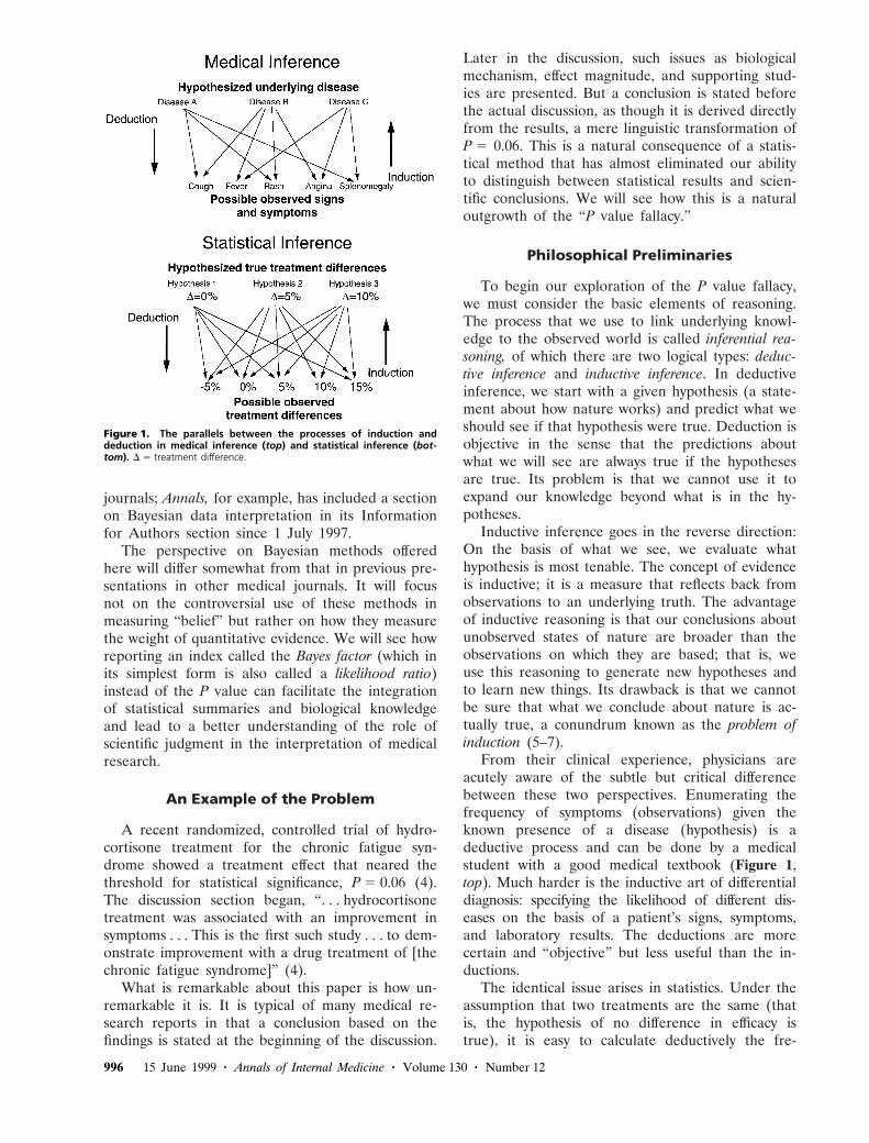
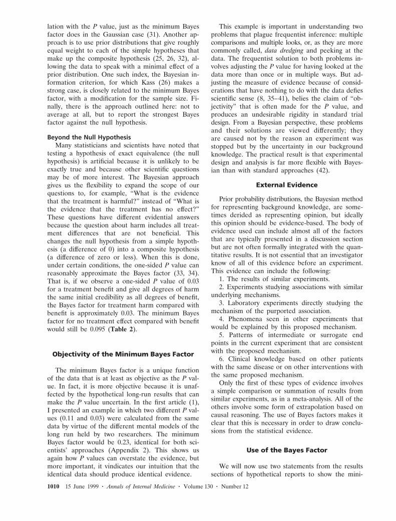
From their clinical experience, physicians areacutely aware of the subtle but critical differencebetween these two perspectives. Enumerating thefrequency of symptoms (observations) given theknown presence of a disease (hypothesis) is adeductive process and can be done by a medicalstudent with a good medical textbook (Figure 1,top). Much harder is the inductive art of differentialdiagnosis: specifying the likelihood of different dis-eases on the basis of a patient’s signs, symptoms,and laboratory results. The deductions are morecertain and “objective” but less useful than the in-ductions.

The identical issue arises in statistics. Under theassumption that two treatments are the same (thatis, the hypothesis of no difference in efficacy istrue), it is easy to calculate deductively the fre-

Figure 1. The parallels between the processes of induction anddeduction in medical inference (top) and statistical inference (bot-tom). D 5 treatment difference.

996 15 June 1999 • Annals of Internal Medicine • Volume 130 • Number 12

quency of all possible outcomes that we could ob-serve in a study (Figure 1, bottom). But once weobserve a particular outcome, as in the result of aclinical trial, it is not easy to answer the moreimportant inductive question, “How likely is it thatthe treatments are equivalent?”

In this century, philosophers have grappled withthe problem of induction and have tried to solve orevade it in several ways. Karl Popper (8) proposeda philosophy of scientific practice that eliminatedformal induction completely and used only the de-ductive elements of science: the prediction and fal-sification components. Rudolf Carnap tried an op-posite strategy—to make the inductive componentas logically secure as the deductive part (9, 10).Both were unsuccessful in producing workable mod-els for how science could be conducted, and theirfailures showed that there is no methodologic solu-tion to the problem of fallible scientific knowledge.

Determining which underlying truth is most likelyon the basis of the data is a problem in inverseprobability, or inductive inference, that was solvedquantitatively more than 200 years ago by the Rev-erend Thomas Bayes. He withheld his discovery,now known as Bayes theorem; it was not divulgeduntil 1762, 20 years after his death (11). Figure 2shows Bayes theorem in words.

As a mathematical equation, Bayes theorem isnot controversial; it serves as the foundation foranalyzing games of chance and medical screeningtests. However, as a model for how we should thinkscientifically, it is criticized because it requires assign-ing a prior probability to the truth of an idea, anumber whose objective scientific meaning is un-clear (7, 10, 12). It is speculated that this may bewhy Reverend Bayes chose the more dire of the“publish or perish” options. It is also the reasonwhy this approach has been tarred with the “sub-jective” label and has not generally been used bymedical researchers.

Conventional (Frequentist)Statistical Inference

Because of the subjectivity of the prior probabil-ities used in Bayes theorem, scientists in the 1920sand 1930s tried to develop alternative approaches to

statistical inference that used only deductive proba-bilities, calculated with mathematical formulas thatdescribed (under certain assumptions) the frequencyof all possible experimental outcomes if an experi-ment were repeated many times (10). Methods basedon this “frequentist” view of probability included anindex to measure the strength of evidence called theP value, proposed by R.A. Fisher in the 1920s (13),and a method for choosing between hypotheses,called a hypothesis test, developed in the early 1930sby the mathematical statisticians Jerzy Neyman andEgon Pearson (14). These two methods were incom-patible but have become so intertwined that they aremistakenly regarded as part of a single, coherent ap-proach to statistical inference (6, 15, 16).

The P Value

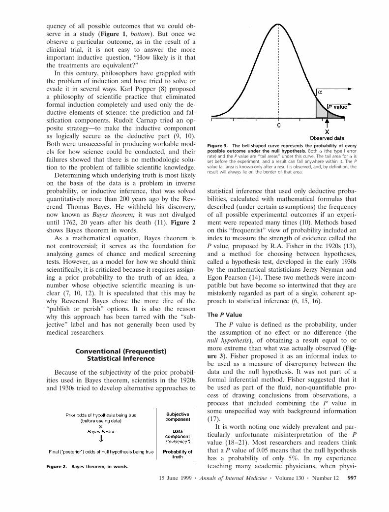
The P value is defined as the probability, underthe assumption of no effect or no difference (thenull hypothesis), of obtaining a result equal to ormore extreme than what was actually observed (Fig-ure 3). Fisher proposed it as an informal index tobe used as a measure of discrepancy between thedata and the null hypothesis. It was not part of aformal inferential method. Fisher suggested that itbe used as part of the fluid, non-quantifiable pro-cess of drawing conclusions from observations, aprocess that included combining the P value insome unspecified way with background information(17).

It is worth noting one widely prevalent and par-ticularly unfortunate misinterpretation of the Pvalue (18–21). Most researchers and readers thinkthat a P value of 0.05 means that the null hypothesishas a probability of only 5%. In my experienceteaching many academic physicians, when physi-Figure 2. Bayes theorem, in words.

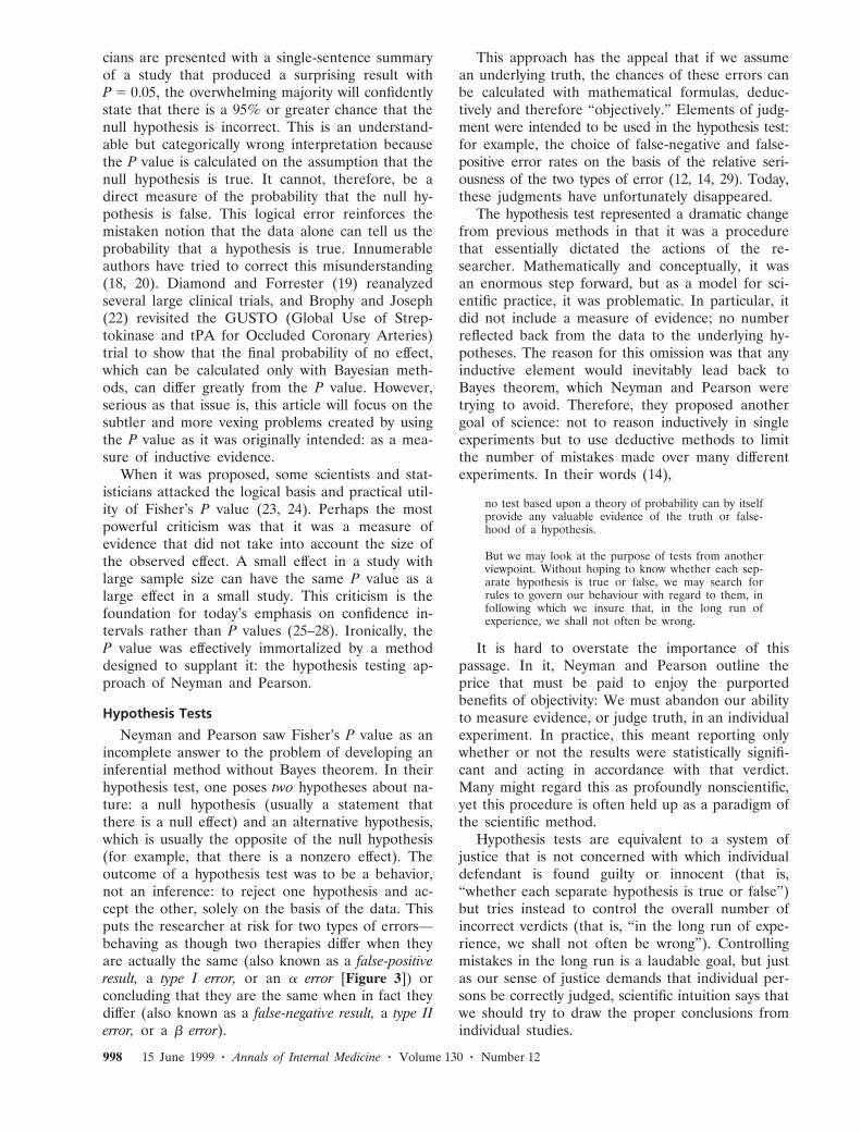
Figure 3. The bell-shaped curve represents the probability of everypossible outcome under the null hypothesis. Both a (the type I errorrate) and the P value are “tail areas” under this curve. The tail area for a isset before the experiment, and a result can fall anywhere within it. The Pvalue tail area is known only after a result is observed, and, by definition, theresult will always lie on the border of that area.

15 June 1999 • Annals of Internal Medicine • Volume 130 • Number 12 997

cians are presented with a single-sentence summaryof a study that produced a surprising result withP 5 0.05, the overwhelming majority will confidentlystate that there is a 95% or greater chance that thenull hypothesis is incorrect. This is an understand-able but categorically wrong interpretation becausethe P value is calculated on the assumption that thenull hypothesis is true. It cannot, therefore, be adirect measure of the probability that the null hy-pothesis is false. This logical error reinforces themistaken notion that the data alone can tell us theprobability that a hypothesis is true. Innumerableauthors have tried to correct this misunderstanding(18, 20). Diamond and Forrester (19) reanalyzedseveral large clinical trials, and Brophy and Joseph(22) revisited the GUSTO (Global Use of Strep-tokinase and tPA for Occluded Coronary Arteries)trial to show that the final probability of no effect,which can be calculated only with Bayesian meth-ods, can differ greatly from the P value. However,serious as that issue is, this article will focus on thesubtler and more vexing problems created by usingthe P value as it was originally intended: as a mea-sure of inductive evidence.

When it was proposed, some scientists and stat-isticians attacked the logical basis and practical util-ity of Fisher’s P value (23, 24). Perhaps the mostpowerful criticism was that it was a measure ofevidence that did not take into account the size ofthe observed effect. A small effect in a study withlarge sample size can have the same P value as alarge effect in a small study. This criticism is thefoundation for today’s emphasis on confidence in-tervals rather than P values (25–28). Ironically, theP value was effectively immortalized by a methoddesigned to supplant it: the hypothesis testing ap-proach of Neyman and Pearson.

Hypothesis Tests

Neyman and Pearson saw Fisher’s P value as anincomplete answer to the problem of developing aninferential method without Bayes theorem. In theirhypothesis test, one poses two hypotheses about na-ture: a null hypothesis (usually a statement thatthere is a null effect) and an alternative hypothesis,which is usually the opposite of the null hypothesis(for example, that there is a nonzero effect). Theoutcome of a hypothesis test was to be a behavior,not an inference: to reject one hypothesis and ac-cept the other, solely on the basis of the data. Thisputs the researcher at risk for two types of errors—behaving as though two therapies differ when theyare actually the same (also known as a false-positiveresult, a type I error, or an a error [Figure 3]) orconcluding that they are the same when in fact theydiffer (also known as a false-negative result, a type IIerror, or a b error).

This approach has the appeal that if we assumean underlying truth, the chances of these errors canbe calculated with mathematical formulas, deduc-tively and therefore “objectively.” Elements of judg-ment were intended to be used in the hypothesis test:for example, the choice of false-negative and false-positive error rates on the basis of the relative seri-ousness of the two types of error (12, 14, 29). Today,these judgments have unfortunately disappeared.

The hypothesis test represented a dramatic changefrom previous methods in that it was a procedurethat essentially dictated the actions of the re-searcher. Mathematically and conceptually, it wasan enormous step forward, but as a model for sci-entific practice, it was problematic. In particular, itdid not include a measure of evidence; no numberreflected back from the data to the underlying hy-potheses. The reason for this omission was that anyinductive element would inevitably lead back toBayes theorem, which Neyman and Pearson weretrying to avoid. Therefore, they proposed anothergoal of science: not to reason inductively in singleexperiments but to use deductive methods to limitthe number of mistakes made over many differentexperiments. In their words (14),

no test based upon a theory of probability can by itselfprovide any valuable evidence of the truth or false-hood of a hypothesis.

But we may look at the purpose of tests from anotherviewpoint. Without hoping to know whether each sep-arate hypothesis is true or false, we may search forrules to govern our behaviour with regard to them, infollowing which we insure that, in the long run ofexperience, we shall not often be wrong.

It is hard to overstate the importance of thispassage. In it, Neyman and Pearson outline theprice that must be paid to enjoy the purportedbenefits of objectivity: We must abandon our abilityto measure evidence, or judge truth, in an individualexperiment. In practice, this meant reporting onlywhether or not the results were statistically signifi-cant and acting in accordance with that verdict.Many might regard this as profoundly nonscientific,yet this procedure is often held up as a paradigm ofthe scientific method.

Hypothesis tests are equivalent to a system ofjustice that is not concerned with which individualdefendant is found guilty or innocent (that is,“whether each separate hypothesis is true or false”)but tries instead to control the overall number ofincorrect verdicts (that is, “in the long run of expe-rience, we shall not often be wrong”). Controllingmistakes in the long run is a laudable goal, but justas our sense of justice demands that individual per-sons be correctly judged, scientific intuition says thatwe should try to draw the proper conclusions fromindividual studies.


The hypothesis test approach offered scientists aFaustian bargain—a seemingly automatic way tolimit the number of mistaken conclusions in thelong run, but only by abandoning the ability tomeasure evidence and assess truth from a singleexperiment. It is doubtful that hypothesis testswould have achieved their current degree of accep-tance if something had not been added that letscientists mistakenly think they could avoid thattrade-off. That something turned out to be Fisher’s“P value,” much to the dismay of Fisher, Neyman,Pearson, and many experts on statistical inferencewho followed.

The P Value “Solution”

How did the P value seem to solve an insolubleproblem? It did so in part by appearing to be ameasure of evidence in a single experiment that didnot violate the long-run logic of the hypothesis test.Figure 3 shows how similar the P value and the avalue (the false-positive error rate) appear. Both aretail-area probabilities under the null hypothesis. Thetail area corresponding to the false-positive errorrate (a) of the hypothesis test is fixed before theexperiment begins (almost always at 0.05), whereasthe P value tail area starts from a point determinedby the data. Their superficial similarity makes iteasy to conclude that the P value is a special kind offalse-positive error rate, specific to the data in hand.In addition, using Fisher’s logic that the P valuemeasured how severely the null hypothesis was con-tradicted by the data (that is, it could serve as ameasure of evidence against the null hypothesis), wehave an index that does double duty. It seems to bea Neyman–Pearson data-specific, false-positive errorrate and a Fisher measure of evidence against thenull hypothesis (6, 15, 17).

A typical passage from a standard biostatisticstext, in which the type I error rate is called a“significance level,” shows how easily the connectionbetween the P value and the false-positive error rateis made (30):

The statement “P , 0.01” indicates that the discrep-ancy between the sample mean and the null hypothesismean is significant even if such a conservative signifi-cance level as 1 percent is adopted. The statement“P 5 0.006” indicates that the result is significant atany level up to 0.6 percent.

The plausibility of this dual evidence/error-rateinterpretation is bolstered by our intuition that themore evidence our conclusions are based on, theless likely we are to be in error. This intuition iscorrect, but the question is whether we can use asingle number, a probability, to represent both thestrength of the evidence against the null hypothesis

and the frequency of false-positive error under thenull hypothesis. If so, then Neyman and Pearsonmust have erred when they said that we could notboth control long-term error rates and judgewhether conclusions from individual experimentswere true. But they were not wrong; it is not logi-cally possible.

The P Value Fallacy

The idea that the P value can play both of theseroles is based on a fallacy: that an event can beviewed simultaneously both from a long-run and ashort-run perspective. In the long-run perspective,which is error-based and deductive, we group theobserved result together with other outcomes thatmight have occurred in hypothetical repetitions ofthe experiment. In the “short run” perspective,which is evidential and inductive, we try to eval-uate the meaning of the observed result from asingle experiment. If we could combine these per-spectives, it would mean that inductive ends(drawing scientific conclusions) could be servedwith purely deductive methods (objective proba-bility calculations).

These views are not reconcilable because a givenresult (the short run) can legitimately be included inmany different long runs. A classic statistical puzzledemonstrating this involves two treatments, A andB, whose effects are contrasted in each of six pa-tients. Treatment A is better in the first five patientsand treatment B is superior in the sixth patient.Adopting Royall’s formulation (6), let us imaginethat this experiment were conducted by two inves-tigators, each of whom, unbeknownst to the other,had a different plan for the experiment. An inves-tigator who originally planned to study six patientswould calculate a P value of 0.11, whereas one whoplanned to stop as soon as treatment B was pre-ferred (up to a maximum of six patients) wouldcalculate a P value of 0.03 (Appendix). We have thesame patients, the same treatments, and the sameoutcomes but two very different P values (whichmight produce different conclusions), which differonly because the experimenters have differentmental pictures of what the results could be if theexperiment were repeated. A confidence intervalwould show this same behavior.

This puzzling and disturbing result comes fromthe attempt to describe long-run behavior and short-run meaning by using the same number. Figure 4illustrates all of the outcomes that could have oc-curred under the two investigators’ plans for theexperiment: that is, in the course of the long run ofeach design. The long runs of the two designs differgreatly and in fact have only two possible results incommon: the observed one and the six treatment A


preferences. When we group the observed resultwith results from the different long runs, we get twodifferent P values (Appendix).

Another way to explain the P value fallacy is thata result cannot at the same time be an anonymous(interchangeable) member of a group of results (thelong-run view) and an identifiable (unique) member(the short-run view) (6, 15, 31). In my second articlein this issue, we will see that if we stick to theshort-run perspective when measuring evidence,identical data produce identical evidence regardlessof the experimenters’ intentions.

Almost every situation in which it is difficult tocalculate the “correct” P value is grounded in thisfundamental problem. The multiple comparisons de-bate is whether a comparison should be consideredpart of a group of all comparisons made (that is, asan anonymous member) or separately (as an iden-tifiable member) (32–35). The controversy over howto cite a P value when a study is stopped because ofa large treatment effect is about whether we con-sider the result alone or as part of all results thatmight have arisen from such monitoring (36–39). Ina trial of extracorporeal membrane oxygenation ininfants, a multitude of P values were derived fromthe same data (40). This problem also has implica-tions for the design of experiments. Because fre-quentist inference requires the “long run” to beunambiguous, frequentist designs need to be rigid(for example, requiring fixed sample sizes and pre-specified stopping rules), features that many regardas requirements of science rather than as artifacts ofa particular inferential philosophy.

The P value, in trying to serve two roles, servesneither one well. This is seen by examining thestatement that “a result with P 5 0.05 is in agroup of outcomes that has a 5% chance of oc-

curring under the null hypothesis.” Although thatis literally the case, we know that the result is notjust in that group (that is, anonymous); we knowwhere it is, and we know that it is the mostprobable member (that is, it is identifiable). It isin that group in the same way that a student whoranks 10 out of 100 is in the top 10% of the class,or one who ranks 20th is in the top 20% (15).Although literally true, these statements are decep-tive because they suggest that a student could beanywhere in a top fraction when we know he or sheis at the lowest level of that top group. This sameproperty is part of what makes the P value aninappropriate measure of evidence against the nullhypothesis. As will be explored in some depth in thesecond article, the evidential strength of a resultwith a P value of 0.05 is actually much weaker thanthe number 0.05 suggests.

If the P value fallacy were limited to the realm ofstatistics, it would be a mere technical footnote,hardly worth an extended exposition. But like asingle gene whose abnormality can disrupt the func-tioning of a complex organism, the P value fallacyallowed the creation of a method that amplified thefallacy into a conceptual error that has profoundlyinfluenced how we think about the process of sci-ence and the nature of scientific truth.

Creation of a Combined Method

The structure of the P value and the subtlety ofthe fallacy that it embodied enabled the combina-tion of the hypothesis test and P value approaches.This combination method is characterized by settingthe type I error rate (almost always 5%) and power(almost always $80%) before the experiment, thencalculating a P value and rejecting the null hypoth-esis if the P value is less than the preset type I errorrate.

The combined method appears, completely de-ductively, to associate a probability (the P value)with the null hypothesis within the context of amethod that controls the chances of errors. The keyword here is probability, because a probability hasan absoluteness that overwhelms caveats that it isnot a probability of truth or that it should not beused mechanically. Such features as biological plau-sibility, the cogency of the theory being tested, andthe strength of previous results all become mereside issues of unclear relevance. None of thesechange the probability, and the probability does notneed them for interpretation. Thus, we have anobjective inference calculus that manufactures con-clusions seemingly without paying Neyman andPearson’s price (that is, that it not be used to drawconclusions from individual studies) and without

Figure 4. Possible outcomes of two hypothetical trials in six pa-tients (Appendix). The only possible overlapping results are the observeddata and the result in which treatment A was preferred in all patients.


Fisher’s flexibility (that is, that background knowl-edge be incorporated).

In didactic articles in the biomedical literature,the fusion of the two approaches is so complete thatsometimes no combination is recognized at all; theP value is identified as equivalent to the chance ofa false-positive error. In a tutorial on statistics forsurgeons, under the unwittingly revealing subhead-ing of “Errors in statistical inference,” we are toldthat “Type I error is incurred if Ho [the null hy-pothesis] is falsely rejected, and the probability ofthis corresponds to the familiar P-value” (41).

The originators of these approaches—Fisher,Neyman, and Pearson—were acutely aware of theimplications of their methods for science, and whilethey each fought for their own approaches in adebate characterized by rhetorical vehemence andsometimes personal attacks (15, 16), neither sidecondoned the combined method. However, the twoapproaches somehow were blended into a receivedmethod whose internal inconsistencies and concep-tual limitations continue to be widely ignored. Manysources on statistical theory make the distinctionsoutlined here (42–45), but in applied texts andmedical journals, the combined method is typicallypresented anonymously as an abstract mathematicaltruth, rarely with a hint of any controversy. Of note,because the combined method is not a coherentbody of ideas, it has been adapted in different formsin diverse applied disciplines, such as psychology,physics, economics, and genetic epidemiology (16).

A natural question is, What drove this method tobe so widely promoted and accepted within medi-cine and other disciplines? Although the scholarshipaddressing that question is not yet complete, recentbooks by Marks (46), Porter (47), Matthews (48),and Gigerenzer and colleagues (16) have identifiedroles for both scientific and sociologic forces. It is acomplex story, but the basic theme is that therapeu-tic reformers in academic medicine and in govern-ment, along with medical researchers and journaleditors, found it enormously useful to have a quan-titative methodology that ostensibly generated con-clusions independent of the persons performing theexperiment. It was believed that because the methodswere “objective,” they necessarily produced reliable,“scientific” conclusions that could serve as the basesfor therapeutic decisions and government policy.

This method thus facilitated a subtle change inthe balance of medical authority from those withknowledge of the biological basis of medicine to-ward those with knowledge of quantitative methods,or toward the quantitative results alone, as thoughthe numbers somehow spoke for themselves. This ismanifest today in the rise of the evidence-basedmedicine paradigm, which occasionally raises hack-les by suggesting that information about biological

mechanisms does not merit the label “evidence”when medical interventions are evaluated (49–51).

Implications for Interpretation ofMedical Research

This combined method has resulted in an auto-maticity in interpreting medical research results thatclinicians, statisticians, and methodology-orientedresearchers have decried over the years (18, 52–68).As A.W.F. Edwards, a statistician, geneticist, andprotege of R.A. Fisher, trenchantly observed,

What used to be called judgment is now called preju-dice, and what used to be called prejudice is nowcalled a null hypothesis . . . it is dangerous nonsense(dressed up as the ‘scientific method’) and will causemuch trouble before it is widely appreciated as such(69).

Another statistician worried about the “unintention-al brand of tyranny” that statistical procedures ex-ercise over other ways of thinking (70).

The consequence of this “tyranny” is weakeneddiscussion sections in research articles, with back-ground information and previous empirical evidenceintegrated awkwardly, if at all, with the statisticalresults. A recent study of randomized, controlledtrials reported in major medical journals showedthat very few referred to the body of previous evi-dence from such trials in the same field (71). This isthe natural result of a methodology that suggeststhat each study alone generates conclusions withcertain error rates instead of adding evidence tothat provided by other sources and other studies.

The example presented at the start of this articlewas not chosen because it was unusually flawed butbecause it was a typical example of how this prob-lem manifests in the medical literature. The state-ment that there was a relation between hydrocorti-sone treatment and improvement of the chronicfatigue syndrome was a knowledge claim, an induc-tive inference. To make such a claim, a bridge mustbe constructed between “P 5 0.06” and “treatmentwas associated with improvement in symptoms.”That bridge consists of everything that the authorsput into the latter part of their discussion: the mag-nitude of the change (small), the failure to changeother end points, the absence of supporting studies,and the weak support for the proposed biologicalmechanism. Ideally, all of this other informationshould have been combined with the modest statis-tical evidence for the main end point to generate aconclusion about the likely presence or absence of atrue hydrocortisone effect. The authors did recom-mend against the use of the treatment, primarilybecause the risk for adrenal suppression could out-weigh the small beneficial effect, but the claim forthe benefit of hydrocortisone remained.


Another interesting feature of that presentationwas that the magnitude of the P value seemed toplay almost no role. The initial conclusion wasphrased no differently than if the P value had beenless than 0.001. This omission is the legacy of thehypothesis test component of the combined methodof inference. The authors (and journal) are to belauded for not hewing rigidly to hypothesis testlogic, which would dismiss the P value of 0.06 asnonsignificant, but if one does not use the hypoth-esis test framework, conclusions must incorporatethe graded nature of the evidence. Unfortunately,even Fisher could offer little guidance on how thesize of a P value should affect a conclusion, andneither has anyone else. In contrast, we will see inthe second article how Bayes factors offer a naturalway to incorporate different grades of evidence intothe formation of conclusions.

In practice, what is most often done to make theleap from evidence to inference is that differentverbal labels are assigned to P values, a practicewhose incoherence is most apparent when the “sig-nificance” verdict is not consistent with external ev-idence or the author’s beliefs. If a P value of 0.12 isfound for an a priori unsuspected difference, anauthor often says that the groups are “equivalent”or that there was “no difference.” But the same Pvalue found for an expected difference results in theuse of words such as “trend” or “suggestion,” aclaim that the study was “not significant because ofsmall sample size,” or an intensive search for alter-native explanations. On the other hand, an unex-pected result with a P value of 0.01 may be declareda statistical fluke arising from data dredging orperhaps uncontrolled confounding. Perhaps worst isthe practice that is most common: accepting at facevalue the significance verdict as a binary indicator ofwhether or not a relation is real. What drives all ofthese practices is a perceived need to make it ap-pear that conclusions are being drawn directly fromthe data, without any external influence, becausedirect inference from data to hypothesis is thoughtto result in mistaken conclusions only rarely and istherefore regarded as “scientific.” This idea is rein-forced by a methodology that puts numbers—astamp of legitimacy—on that misguided approach.

Many methodologic disputes in medical research,such as those around multiple comparisons, whethera hypothesis was thought of before or after seeingthe data, whether an endpoint is primary or second-ary, or how to handle multiple looks at accumulatingdata, are actually substantive scientific disagreementsthat have been converted into pseudostatistical de-bates. The technical language and substance ofthese debates often exclude the investigators whomay have the deepest insight into the biologicalissues. A vivid example is found in a recent series of

articles reporting on a U.S. Food and Drug Admin-istration committee debate on the approval ofcarvedilol, a cardiovascular drug, in which the dis-cussion focused on whether (and which) statistical“rules” had been broken (72–74). Assessing anddebating the cogency of disparate real-world sourcesof laboratory and clinical evidence are the heart ofscience, and conclusions can be drawn only whenthat assessment is combined with statistical results.The combination of hypothesis testing and P valuesoffers no way to accomplish this critical task.

Proposed Solutions

Various remedies to the problems discussed thusfar have been proposed (18, 52–67). Most involvemore use of confidence intervals and various allot-ments of common sense. Confidence intervals, de-rived from the same frequentist mathematics as hy-pothesis tests, represent the range of effects that are“compatible with the data.” Their chief asset is that,ideally, they push us away from the automaticity ofP values and hypothesis tests by promoting a con-sideration of the size of the observed effect. Theyare cited more often in medical research reportstoday than in the past, but their impact on theinterpretation of research is less clear. Often, theyare used simply as surrogates for the hypothesis test(75); researchers simply see whether they includethe null effect rather than consider the clinical im-plications of the full range of likely effect size. Thefew efforts to eliminate P values from journals infavor of confidence intervals have not generallybeen successful, indicating that researchers’ needfor a measure of evidence remains strong and thatthey often feel lost without one (76, 77). But con-fidence intervals are far from a panacea; they em-body, albeit in subtler form, many of the sameproblems that afflict current methods (78), the mostimportant being that they offer no mechanism tounite external evidence with that provided by anexperiment. Thus, although confidence intervals area step in the right direction, they are not a solutionto the most serious problem created by frequentistmethods. Other recommended solutions have in-cluded likelihood or Bayesian methods (6, 19, 20,79–84). The second article will explore the use ofBayes factor—the Bayesian measure of evidence—and show how this approach can change not onlythe numbers we report but, more important, howwe think about them.

A Final Note

Some of the strongest arguments in support ofstandard statistical methods is that they are a greatimprovement over the chaos that preceded them


and that they have proved enormously useful inpractice. Both of these are true, in part becausestatisticians, armed with an understanding of thelimitations of traditional methods, interpret quanti-tative results, especially P values, very differentlyfrom how most nonstatisticians do (67, 85, 86). Butin a world where medical researchers have access toincreasingly sophisticated statistical software, thestatistical complexity of published research is in-creasing (87–89), and more clinical care is beingdriven by the empirical evidence base, a deeperunderstanding of statistics has become too impor-tant to leave only to statisticians.

Appendix: Calculation of P Value in a TrialInvolving Six Patients

Null hypothesis: Probability that treatment A is bet-ter 5 1/2

The n 5 6 design: The probability of the observed re-sult (one treatment B success and five treatment A suc-cesses) is 6 3 (1/2) 3 (1/2)5. The factor “6” appearsbecause the success of treatment B could have occurredin any of the six patients. The more extreme result wouldbe the one in which treatment A was superior in all sixpatients, with a probability (under the null hypothesis) of(1/2)6. The one-sided P value is the sum of those twoprobabilities:

“Stop at first treatment B preference” design: The possi-ble results of such an experiment would be either a singleinstance of preference for treatment B or successivelymore preferences for treatment A, followed by a case ofpreference for treatment B, up to a total of six instances.With the same data as before, the probability of theobserved result of 5 treatment A preferences 2 1 treat-ment B preference would be (1/2)5 3 (1/2) (without thefactor of “6” because the preference for treatment B mustalways fall at the end) and the more extreme result wouldbe six preferences for treatment As, as in the other de-sign. The one-sided P value is:

Requests for Reprints: Steven Goodman, MD, PhD, Johns Hop-kins University, 550 North Broadway, Suite 409, Baltimore, MD21205; e-mail, [email protected].

References

1. Simon R, Altman DG. Statistical aspects of prognostic factor studies inoncology [Editorial]. Br J Cancer. 1994;69:979-85.

2. Tannock IF. False-positive results in clinical trials: multiple significance testsand the problem of unreported comparisons. J Natl Cancer Inst. 1996;88:206-7.

3. Goodman SN. Toward evidence-based medical statistics. 2: The Bayes factor.Ann Intern Med. 1999;130:1005-13.

4. McKenzie R, O’Fallon A, Dale J, Demitrack M, Sharma G, Deloria M, etal. Low-dose hydrocortisone for treatment of chronic fatigue syndrome: arandomized controlled trial. JAMA. 1998;280:1061-6.

5. Salmon WC. The Foundations of Scientific Inference. Pittsburgh: Univ ofPittsburgh Pr; 1966.

6. Royall R. Statistical Evidence: A Likelihood Primer. Monographs on Statisticsand Applied Probability #71. London: Chapman and Hall; 1997.

7. Hacking I. The Emergence of Probability: A Philosophical Study of Early Ideasabout Probability, Induction and Statistical Inference. Cambridge, UK: Cam-bridge Univ Pr; 1975.

8. Popper K. The Logic of Scientific Discovery. New York: Harper & Row; 1934:59.9. Carnap R. Logical Foundations of Probability. Chicago: Univ of Chicago Pr;

1950.10. Howson C, Urbach P. Scientific Reasoning: The Bayesian Approach. 2d ed.

La Salle, IL: Open Court; 1993.11. Stigler SM. The History of Statistics: The Measurement of Uncertainty before

1900. Cambridge, MA: Harvard Univ Pr; 1986.12. Oakes M. Statistical Inference: A Commentary for the Social Sciences. New

York: Wiley; 1986.13. Fisher R. Statistical Methods for Research Workers. 13th ed. New York:

Hafner; 1958.14. Neyman J, Pearson E. On the problem of the most efficient tests of statis-

tical hypotheses. Philosophical Transactions of the Royal Society, Series A.1933;231:289-337.

15. Goodman SN. p values, hypothesis tests, and likelihood: implications forepidemiology of a neglected historical debate. Am J Epidemiol. 1993;137:485-96.

16. Gigerenzer G, Swijtink Z, Porter T, Daston L, Beatty J, Kruger L. TheEmpire of Chance. Cambridge, UK: Cambridge Univ Pr; 1989.

17. Fisher R. Statistical Methods and Scientific Inference. 3d ed. New York:Macmillan; 1973.

18. Browner W, Newman T. Are all significant P values created equal? Theanalogy between diagnostic tests and clinical research. JAMA. 1987;257:2459-63.

19. Diamond GA, Forrester JS. Clinical trials and statistical verdicts: probablegrounds for appeal. Ann Intern Med. 1983;98:385-94.

20. Lilford RJ, Braunholtz D. For debate: The statistical basis of public policy: aparadigm shift is overdue. BMJ. 1996;313:603-7.

21. Freeman PR. The role of p-values in analysing trial results. Stat Med. 1993;12:1442-552.

22. Brophy JM, Joseph L. Placing trials in context using Bayesian analysis.GUSTO revisited by Reverend Bayes. JAMA. 1995;273:871-5.

23. Berkson J. Tests of significance considered as evidence. Journal of the Amer-ican Statistical Association. 1942;37:325-35.

24. Pearson E. ’Student’ as a statistician. Biometrika. 1938;38:210-50.25. Altman DG. Confidence intervals in research evaluation. ACP J Club. 1992;

Suppl 2:A28-9.26. Berry G. Statistical significance and confidence intervals [Editorial]. Med J

Aust. 1986;144:618-9.27. Braitman LE. Confidence intervals extract clinically useful information from

data [Editorial]. Ann Intern Med. 1988;108:296-8.28. Simon R. Confidence intervals for reporting results of clinical trials. Ann

Intern Med. 1986;105:429-35.29. Pearson E. Some thoughts on statistical inference. Annals of Mathematical

Statistics. 1962;33:394-403.30. Colton T. Statistics in Medicine. Boston: Little, Brown; 1974.31. Seidenfeld T. Philosophical Problems of Statistical Inference. Dordrecht, the

Netherlands: Reidel; 1979.32. Goodman S. Multiple comparisons, explained. Am J Epidemiol. 1998;147:

807-12.33. Savitz DA, Olshan AF. Multiple comparisons and related issues in the in-

terpretation of epidemiologic data. Am J Epidemiol. 1995;142:904-8.34. Thomas DC, Siemiatycki J, Dewar R, Robins J, Goldberg M, Armstrong

BG. The problem of multiple inference in studies designed to generate hy-potheses. Am J Epidemiol. 1985;122:1080-95.

35. Greenland S, Robins JM. Empirical-Bayes adjustments for multiple compar-isons are sometimes useful. Epidemiology. 1991;2:244-51.

36. Anscombe F. Sequential medical trials. Journal of the American StatisticalAssociation. 1963;58:365-83.

37. Dupont WD. Sequential stopping rules and sequentially adjusted P values:does one require the other? Controlled Clin Trials. 1983;4:3-10.

38. Cornfield J, Greenhouse S. On certain aspects of sequential clinical trials.Proceedings of the Fifth Berkeley Symposium on Mathematical Statistics andProbability. Berkeley, CA: Univ of California Pr; 1977;4:813-29.

39. Cornfield J. Sequential trials, sequential analysis and the likelihood principle.American Statistician. 1966;20:18-23.

40. Begg C. On inferences from Wei’s biased coin design for clinical trials. Bio-metrika. 1990;77:467-84.

41. Ludbrook J, Dudley H. Issues in biomedical statistics: statistical inference.Aust N Z J Surg. 1994;64:630-6.


42. Cox D, Hinckley D. Theoretical Statistics. New York: Chapman and Hall;1974.

43. Barnett V. Comparative Statistical Inference. New York: Wiley; 1982.44. Lehmann E. The Fisher, Neyman-Pearson theories of testing hypotheses: one

theory or two? Journal of the American Statistical Association. 1993;88:1242-9.

45. Berger J. The frequentist viewpoint and conditioning. In: LeCam L, Olshen R,eds. Proceedings of the Berkeley Conference in Honor of Jerzy Neyman andJack Kiefer. vol. 1. Belmont, CA: Wadsworth; 1985:15-43.

46. Marks HM. The Progress of Experiment: Science and Therapeutic Reform inthe United States, 1900-1990. Cambridge, UK: Cambridge Univ Pr; 1997.

47. Porter TM. Trust In Numbers: The Pursuit of Objectivity in Science and PublicLife. Princeton, NJ: Princeton Univ Pr; 1995.

48. Matthews JR. Quantification and the Quest for Medical Certainty. Princeton,NJ: Princeton Univ Pr; 1995.

49. Feinstein AR, Horwitz RI. Problems in the “evidence” of “evidence-basedmedicine.” Am J Med. 1997;103:529-35.

50. Spodich DH. “Evidence-based medicine”: terminologic lapse or terminologicarrogance? [Letter] Am J Cardiol. 1996;78:608-9.

51. Tonelli MR. The philosophical limits of evidence-based medicine. Acad Med.1998;73:1234-40.

52. Feinstein AR. Clinical Biostatistics. St. Louis: Mosby; 1977.53. Mainland D. The significance of “nonsignificance.” Clin Pharmacol Ther.

1963;12:580-6.54. Morrison DE, Henkel RE. The Significance Test Controversy: A Reader.

Chicago: Aldine; 1970.55. Rothman KJ. Significance questing [Editorial]. Ann Intern Med. 1986;105:

445-7.56. Rozeboom W. The fallacy of the null hypothesis significance test. Psychol

Bull. 1960;57:416-28.57. Savitz D. Is statistical significance testing useful in interpreting data? Reprod

Toxicol. 1993;7:95-100.58. Chia KS. “Significant-itis”—an obsession with the P-value. Scand J Work

Environ Health. 1997;23:152-4.59. Barnett ML, Mathisen A. Tyranny of the p-value: the conflict between

statistical significance and common sense [Editorial]. J Dent Res. 1997;76:534-6.

60. Bailar JC 3d, Mosteller F. Guidelines for statistical reporting in articles formedical journals. Amplifications and explanations. Ann Intern Med. 1988;108:266-73.

61. Cox DR. Statistical significance tests. Br J Clin Pharmacol. 1982;14:325-31.62. Cornfield J. The bayesian outlook and its application. Biometrics. 1969;25:

617-57.63. Mainland D. Statistical ritual in clinical journals: is there a cure?—I. Br Med J

(Clin Res Ed). 1984;288:841-3.64. Mainland D. Statistical ritual in clinical journals: is there a cure?—II. Br Med J

(Clin Res Ed). 1984;288:920-2.65. Salsburg D. The religion of statistics as practiced in medical journals. Amer-

ican Statistician. 1985;39:220-3.

66. Dar R, Serlin RC, Omer H. Misuse of statistical tests in three decades ofpsychotherapy research. J Consult Clin Psychol. 1994;62:75-82.

67. Altman D, Bland J. Improving doctors’ understanding of statistics. Journal ofthe Royal Statistical Society, Series A. 1991;154:223-67.

68. Pocock SJ, Hughes MD, Lee RJ. Statistical problems in the reporting ofclinical trials. A survey of three medical journals. N Engl J Med. 1987;317:426-32.

69. Edwards A. Likelihood. Cambridge, UK: Cambridge Univ Pr; 1972.70. Skellam J. Models, inference and strategy. Biometrics. 1969;25:457-75.71. Clarke M, Chalmers I. Discussion sections in reports of controlled trials

published in general medical journals: islands in search of continents? JAMA.1998;280:280-2.

72. Moye L. End-point interpretation in clinical trials: the case for discipline.Control Clin Trials. 1999;20:40-9.

73. Fisher LD. Carvedilol and the Food and Drug Administration (FDA) approvalprocess: the FDA paradigm and reflections on hypothesis testing. Control ClinTrials. 1999;20:16-39.

74. Fisher L, Moye L. Carvedilol and the Food and Drug Administration (FDA)approval process: an introduction. Control Clin Trials. 1999;20:1-15.

75. Poole C. Beyond the confidence interval. Am J Public Health. 1987;77:195-9.76. Lang JM, Rothman KJ, Cann CI. That confounded P-value [Editorial]. Epi-

demiology. 1998;9:7-8.77. Evans SJ, Mills P, Dawson J. The end of the p value? Br Heart J. 1988;60:

177-80.78. Feinstein AR. P-values and confidence intervals: two sides of the same un-

satisfactory coin. J Clin Epidemiol. 1998;51:355-60.79. Freedman L. Bayesian statistical methods [Editorial]. BMJ. 1996;313:569-70.80. Etzioni RD, Kadane JB. Bayesian statistical methods in public health and

medicine. Annu Rev Public Health. 1995;16:23-41.81. Kadane JB. Prime time for Bayes. Control Clin Trials. 1995;16:313-8.82. Spiegelhalter D, Freedman L, Parmar M. Bayesian approaches to random-

ized trials. Journal of the Royal Statistical Society, Series A. 1994;157:357-87.83. Goodman SN, Royall R. Evidence and scientific research. Am J Public

Health. 1988;78:1568-74.84. Barnard G. The use of the likelihood function in statistical practice. In: Pro-

ceedings of the Fifth Berkeley Symposium. v 1. Berkeley, CA: Univ of Califor-nia Pr; 1966:27-40.

85. Wulff HR, Anderson B, Brandenhoff P, Guttler F. What do doctors knowabout statistics? Stat Med. 1987;6:3-10.

86. Borak J, Veilleux S. Errors of intuitive logic among physicians. Soc Sci Med.1982;16:1939-47.

87. Concato J, Feinstein AE, Holford TR. The risk of determining risk withmultivariable models. Ann Intern Med. 1993;118:201-10.

88. Altman DG, Goodman SN. Transfer of technology from statistical journalsto the biomedical literature. Past trends and future predictions. JAMA. 1994;272:129-32.

89. Hayden G. Biostatistical trends in pediatrics: implications for the future.Pediatrics. 1983;72:84-7.


Toward Evidence-Based Medical Statistics. 2: The Bayes FactorSteven N. Goodman, MD, PhD

Bayesian inference is usually presented as a method fordetermining how scientific belief should be modified bydata. Although Bayesian methodology has been one ofthe most active areas of statistical development in the past20 years, medical researchers have been reluctant to em-brace what they perceive as a subjective approach to dataanalysis. It is little understood that Bayesian methods havea data-based core, which can be used as a calculus ofevidence. This core is the Bayes factor, which in its simplestform is also called a likelihood ratio. The minimum Bayesfactor is objective and can be used in lieu of the P value asa measure of the evidential strength. Unlike P values,Bayes factors have a sound theoretical foundation and aninterpretation that allows their use in both inference anddecision making. Bayes factors show that P values greatlyoverstate the evidence against the null hypothesis. Mostimportant, Bayes factors require the addition of backgroundknowledge to be transformed into inferences—probabilitiesthat a given conclusion is right or wrong. They make thedistinction clear between experimental evidence and infer-ential conclusions while providing a framework in which tocombine prior with current evidence.

This paper is also available at http://www.acponline.org.

Ann Intern Med. 1999;130:1005-1013.

From Johns Hopkins University School of Medicine, Baltimore,Maryland. For the current author address, see end of text.

In the first of two articles on evidence-based sta-tistics (1), I outlined the inherent difficulties of

the standard frequentist statistical approach to in-ference: problems with using the P value as a mea-sure of evidence, internal inconsistencies of the com-bined hypothesis test–P value method, and how thatmethod inhibits combining experimental results withbackground information. Here, I explore, as non-mathematically as possible, the Bayesian approachto measuring evidence and combining informationand epistemologic uncertainties that affect all statis-tical approaches to inference. Some of this presen-tation may be new to clinical researchers, but mostof it is based on ideas that have existed at least sincethe 1920s and, to some extent, centuries earlier (2).

The Bayes Factor Alternative

Bayesian inference is often described as amethod of showing how belief is altered by data.Because of this, many researchers regard it as non-scientific; that is, they want to know what the datasay, not what our belief should be after observingthem (3). Comments such as the following, which ap-

peared in response to an article proposing a Bayesiananalysis of the GUSTO (Global Utilization of Strep-tokinase and tPA for Occluded Coronary Arteries)trial (4), are typical.

When modern Bayesians include a “prior probabilitydistribution for the belief in the truth of a hypothesis,”they are actually creating a metaphysical model ofattitude change . . . The result . . . cannot be field-testedfor its validity, other than that it “feels” reasonable tothe consumer. . . .

The real problem is that neither classical nor Bayesianmethods are able to provide the kind of answers cli-nicians want. That classical methods are flawed is un-deniable—I wish I had an alternative . . . . (5)

This comment reflects the widespread mispercep-tion that the only utility of the Bayesian approach isas a belief calculus. What is not appreciated is thatBayesian methods can instead be viewed as an evi-dential calculus. Bayes theorem has two compo-nents—one that summarizes the data and one thatrepresents belief. Here, I focus on the componentrelated to the data: the Bayes factor, which in itssimplest form is also called a likelihood ratio. In Bayestheorem, the Bayes factor is the index through whichthe data speak, and it is separate from the purelysubjective part of the equation. It has also been calledthe relative betting odds, and its logarithm is some-times referred to as the weight of the evidence (6, 7).The distinction between evidence and error is clearwhen it is recognized that the Bayes factor (evidence)is a measure of how much the probability of truth(that is, 1 2 prob(error), where prob is probability) isaltered by the data. The equation is as follows:

Prior Oddsof Null Hypothesis 3

BayesFactor 5

Posterior Oddsof Null Hypothesis

where Bayes factor 5

Prob~Data, given the null hypothesis!

Prob~Data, given the alternative hypothesis!

The Bayes factor is a comparison of how welltwo hypotheses predict the data. The hypothesisthat predicts the observed data better is the onethat is said to have more evidence supporting it.Unlike the P value, the Bayes factor has a soundtheoretical foundation and an interpretation that

See related article on pp 995-1004 and editorialcomment on pp 1019-1021.

©1999 American College of Physicians–American Society of Internal Medicine 1005

allows it to be used in both inference and decisionmaking. It links notions of objective probability, ev-idence, and subjective probability into a coherentpackage and is interpretable from all three perspec-tives. For example, if the Bayes factor for the nullhypothesis compared with another hypothesis is 1/2,the meaning can be expressed in three ways.

1. Objective probability: The observed results arehalf as probable under the null hypothesis as theyare under the alternative.

2. Inductive evidence: The evidence supports thenull hypothesis half as strongly as it does the alter-native.

3. Subjective probability: The odds of the nullhypothesis relative to the alternative hypothesis af-ter the experiment are half what they were beforethe experiment.

The Bayes factor differs in many ways from aP value. First, the Bayes factor is not a probabilityitself but a ratio of probabilities, and it can varyfrom zero to infinity. It requires two hypotheses,making it clear that for evidence to be against thenull hypothesis, it must be for some alternative.Second, the Bayes factor depends on the probabilityof the observed data alone, not including unobserved“long run” results that are part of the P value calcu-lation. Thus, factors unrelated to the data that affectthe P value, such as why an experiment was stopped,do not affect the Bayes factor (8, 9).

Because we are so accustomed to thinking of“evidence” and the probability of “error” as synon-ymous, it may be difficult to know how to deal witha measure of evidence that is not a probability. It ishelpful to think of it as analogous to the concept of

energy. We know that energy is real, but because itis not directly observable, we infer the meaning of agiven amount from how much it heats water, lifts aweight, lights a city, or cools a house. We begin tounderstand what “a lot” and “a little” mean throughits effects. So it is with the Bayes factor: It modifiesprior probabilities, and after seeing how muchBayes factors of certain sizes change various priorprobabilities, we begin to understand what repre-sents strong evidence, and weak evidence.

Table 1 shows us how far various Bayes factorsmove prior probabilities, on the null hypothesis, of90%, 50%, and 25%. These correspond, respective-ly, to high initial confidence in the null hypothesis,equivocal confidence, and moderate suspicion thatthe null hypothesis is not true. If one is highly con-vinced of no effect (90% prior probability of thenull hypothesis) before starting the experiment, aBayes factor of 1/10 will move one to being equiv-ocal (47% probability on the null hypothesis), but ifone is equivocal at the start (50% prior probability),that same amount of evidence will be moderately con-vincing that the null hypothesis is not true (9% pos-terior probability). A Bayes factor of 1/100 is strongenough to move one from being 90% sure of thenull hypothesis to being only 8% sure.

As the strength of the evidence increases, thedata are more able to convert a skeptic into abeliever or a tentative suggestion into an acceptedtruth. This means that as the experimental evidencegets stronger, the amount of external evidenceneeded to support a scientific claim decreases. Con-versely, when there is little outside evidence sup-porting a claim, much stronger experimental evidenceis required for it to be credible. This phenomenon canbe observed empirically, in the medical community’sreluctance to accept the results of clinical trials thatrun counter to strong prior beliefs (10, 11).

Bayes Factors and Meta-Analysis

There are two dimensions to the “evidence-based”properties of Bayes factors. One is that they are aproper measure of quantitative evidence; this issuewill be further explored shortly. The other is thatthey allow us to combine evidence from differentexperiments in a natural and intuitive way. To under-stand this, we must understand a little more of thetheory underlying Bayes factors (12–14).

Every hypothesis under which the observed dataare not impossible can be said to have some evi-dence for it. The strength of this evidence is pro-portional to the probability of the data under thathypothesis and is called the likelihood of the hypoth-esis. This use of the term “likelihood” must not beconfused with its common language meaning of

Table 1. Final (Posterior) Probability of the NullHypothesis after Observing Various BayesFactors, as a Function of the Prior Probability ofthe Null Hypothesis

Strengthof Evidence

Bayes Factor Decrease in Probabilityof the Null Hypothesis

From To NoLess Than

%

Weak 1/5 90 64*50 1725 6

Moderate 1/10 90 4750 925 3

Moderate to strong 1/20 90 3150 525 2

Strong to very strong 1/100 90 850 125 0.3

* Calculations were performed as follows:A probability (Prob) of 90% is equivalent to an odds of 9, calculated as Prob/(1 2 Prob).Posterior odds 5 Bayes factor 3 prior odds; thus, (1/5) 3 9 5 1.8.Probability 5 odds/(1 1 odds); thus, 1.8/2.8 5 0.64.


probability (12, 13). Mathematical likelihoods havemeaning only when compared to each other in theform of a ratio (hence, the likelihood ratio), a ratiothat represents the comparative evidential supportgiven to two hypotheses by the data. The likelihoodratio is the simplest form of Bayes factor.

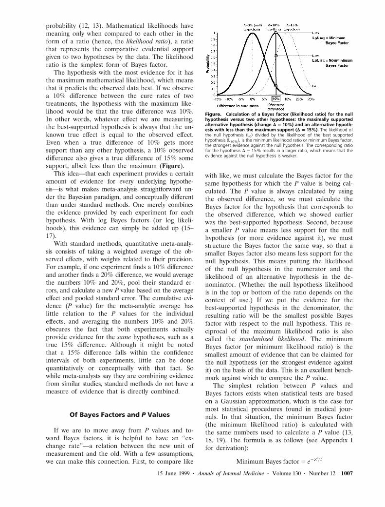
The hypothesis with the most evidence for it hasthe maximum mathematical likelihood, which meansthat it predicts the observed data best. If we observea 10% difference between the cure rates of twotreatments, the hypothesis with the maximum like-lihood would be that the true difference was 10%.In other words, whatever effect we are measuring,the best-supported hypothesis is always that the un-known true effect is equal to the observed effect.Even when a true difference of 10% gets moresupport than any other hypothesis, a 10% observeddifference also gives a true difference of 15% somesupport, albeit less than the maximum (Figure).

This idea—that each experiment provides a certainamount of evidence for every underlying hypothe-sis—is what makes meta-analysis straightforward un-der the Bayesian paradigm, and conceptually differentthan under standard methods. One merely combinesthe evidence provided by each experiment for eachhypothesis. With log Bayes factors (or log likeli-hoods), this evidence can simply be added up (15–17).

With standard methods, quantitative meta-analy-sis consists of taking a weighted average of the ob-served effects, with weights related to their precision.For example, if one experiment finds a 10% differenceand another finds a 20% difference, we would averagethe numbers 10% and 20%, pool their standard er-rors, and calculate a new P value based on the averageeffect and pooled standard error. The cumulative evi-dence (P value) for the meta-analytic average haslittle relation to the P values for the individualeffects, and averaging the numbers 10% and 20%obscures the fact that both experiments actuallyprovide evidence for the same hypotheses, such as atrue 15% difference. Although it might be notedthat a 15% difference falls within the confidenceintervals of both experiments, little can be donequantitatively or conceptually with that fact. Sowhile meta-analysts say they are combining evidencefrom similar studies, standard methods do not have ameasure of evidence that is directly combined.

Of Bayes Factors and P Values

If we are to move away from P values and to-ward Bayes factors, it is helpful to have an “ex-change rate”—a relation between the new unit ofmeasurement and the old. With a few assumptions,we can make this connection. First, to compare like

with like, we must calculate the Bayes factor for thesame hypothesis for which the P value is being cal-culated. The P value is always calculated by usingthe observed difference, so we must calculate theBayes factor for the hypothesis that corresponds tothe observed difference, which we showed earlierwas the best-supported hypothesis. Second, becausea smaller P value means less support for the nullhypothesis (or more evidence against it), we muststructure the Bayes factor the same way, so that asmaller Bayes factor also means less support for thenull hypothesis. This means putting the likelihoodof the null hypothesis in the numerator and thelikelihood of an alternative hypothesis in the de-nominator. (Whether the null hypothesis likelihoodis in the top or bottom of the ratio depends on thecontext of use.) If we put the evidence for thebest-supported hypothesis in the denominator, theresulting ratio will be the smallest possible Bayesfactor with respect to the null hypothesis. This re-ciprocal of the maximum likelihood ratio is alsocalled the standardized likelihood. The minimumBayes factor (or minimum likelihood ratio) is thesmallest amount of evidence that can be claimed forthe null hypothesis (or the strongest evidence againstit) on the basis of the data. This is an excellent bench-mark against which to compare the P value.

The simplest relation between P values andBayes factors exists when statistical tests are basedon a Gaussian approximation, which is the case formost statistical procedures found in medical jour-nals. In that situation, the minimum Bayes factor(the minimum likelihood ratio) is calculated withthe same numbers used to calculate a P value (13,18, 19). The formula is as follows (see Appendix Ifor derivation):

Minimum Bayes factor 5 e2Z2/2

Figure. Calculation of a Bayes factor (likelihood ratio) for the nullhypothesis versus two other hypotheses: the maximally supportedalternative hypothesis (change D 5 10%) and an alternative hypoth-esis with less than the maximum support (D 5 15%). The likelihood ofthe null hypothesis (L0) divided by the likelihood of the best supportedhypothesis (L10%), is the minimum likelihood ratio or minimum Bayes factor,the strongest evidence against the null hypothesis. The corresponding ratiofor the hypothesis D 5 15% results in a larger ratio, which means that theevidence against the null hypothesis is weaker.


where z is the number of standard errors from thenull effect. This formula can also be used if a t-test(substituting t for Z) or a chi-square test (substitut-ing the chi-square value for Z2) is done. The dataare treated as though they came from an experi-ment with a fixed sample size.

This formula allows us to establish an exchangerate between minimum Bayes factors and P valuesin the Gaussian case. Table 2 shows the minimumBayes factor and the standard P value for any givenZ score. For example, when a result is 1.96 standarderrors from its null value (that is, P 5 0.05), theminimum Bayes factor is 0.15, meaning that the nullhypothesis gets 15% as much support as the best-supported hypothesis. This is threefold higher thanthe P value of 0.05, indicating that the evidenceagainst the null hypothesis is not nearly as strong as“P 5 0.05” suggests.

Even when researchers describe results with a Pvalue of 0.05 as being of borderline significance, thenumber “0.05” speaks louder than words, and mostreaders interpret such evidence as much strongerthan it is. These calculations show that P values of0.05 (corresponding to a minimum Bayes factor of0.15) represent, at best, moderate evidence againstthe null hypothesis; those between 0.001 and 0.01represent, at best, moderate to strong evidence; andthose less than 0.001 represent strong to very strongevidence. When the P value becomes very small, thedisparity between it and the minimum Bayes factorbecomes negligible, confirming that strong evidencewill look strong regardless of how it is measured.

The right-hand part of Table 2 uses this relationbetween P values and Bayes factors to show themaximum effect that data with various P values

would have on the plausibility of the null hypothe-sis. If one starts with a chance of no effect of 50%,a result with a minimum Bayes factor of 0.15 (cor-responding to a P value of 0.05) can reduce confi-dence in the null hypothesis to no lower than 13%.The last row in each entry turns the calculationaround, showing how low initial confidence in thenull hypothesis must be to result in 5% confidenceafter seeing the data (that is, 95% confidence in anon-null effect). With a P value of 0.05 (Bayesfactor $ 0.15), the prior probability of the null hy-pothesis must be 26% or less to allow one to con-clude with 95% confidence that the null hypothesisis false. This calculation is not meant to sanctify thenumber “95%” in the Bayesian approach but ratherto show what happens when similar benchmarks areused in the two approaches.

These tables show us what many researcherslearn from experience and what statisticians havelong known; that the weight of evidence against thenull hypothesis is not nearly as strong as the mag-nitude of the P value suggests. This is the main rea-son that many Bayesian reanalyses of clinical trialsconclude that the observed differences are not likelyto be true (4, 20, 21). They conclude this not alwaysbecause contradictory prior evidence outweighedthe trial evidence but because the trial evidence,when measured properly, was not very strong in thefirst place. It also provides justification for the judg-ment of many experienced meta-analysts who havesuggested that the threshold for significance in ameta-analysis should be a result more than twostandard errors from the null effect rather than two(22, 23).

The theory underlying these ideas has a longhistory. Edwards (2) traces the concept of mathe-matical likelihood into the 18th century, althoughthe name and full theoretical development of like-lihood didn’t occur until around 1920, as part ofR.A. Fisher’s theory of maximum likelihood. Thiswas a frequentist theory, however, and Fisher didnot acknowledge the value of using the likelihooddirectly for inference until many years later (24).Edwards (14) and Royall (13) have built on some ofFisher’s ideas, exploring the use of likelihood-basedmeasures of evidence outside of the Bayesian par-adigm. In the Bayesian realm, Jeffreys (25) andGood (6) were among the first to develop the the-ory behind Bayes factors, with the most comprehen-sive recent summary being that of Kass (26). Thesuggestion that the minimum Bayes factor (or min-imum likelihood ratio) could be used as a report-able index appeared in the biomedical literature atleast as early as 1963 (19). The settings in whichBayes factors differ from likelihood ratios are dis-cussed in the following section.

Table 2. Relation between Fixed Sample Size P Valuesand Minimum Bayes Factors and the Effect ofSuch Evidence on the Probability of the NullHypothesis

P Value(Z Score)

MinimumBayes Factor

Decrease in Probability ofthe Null Hypothesis, %

Strength ofEvidence

From To No Less Than

0.10 0.26 75 44 Weak(1.64) (1/3.8) 50 21

17 5

0.05 0.15 75 31 Moderate(1.96) (1/6.8) 50 13

26 5

0.03 0.095 75 22 Moderate(2.17) (1/11) 50 9

33 5

0.01 0.036 75 10 Moderate to strong(2.58) (1/28) 50 3.5

60 5

0.001 0.005 75 1 Strong to very strong(3.28) (1/216) 50 0.5

92 5


Bayes Factors for Composite Hypotheses

Bayes factors larger than the minimum valuescited in the preceding section can be calculated (20,25–27). This is a difficult technical area, but it isimportant to understand in at least a qualitative waywhat these nonminimum Bayes factors measure andhow they differ from simple likelihood ratios.

The definition of the Bayes factor is the proba-bility of the observed data under one hypothesis di-vided by its probability under another hypothesis. Typ-ically, one hypothesis is the null hypothesis of nodifference. The other hypothesis can be stated in manyways, such as “the cure rates differ by 15%.” That iscalled a simple hypothesis because the difference (15%)is specified exactly. The null hypothesis and best-sup-ported hypothesis are both simple hypotheses.

Things get more difficult when we state the al-ternative hypothesis the way it is usually posed: forexample, “the true difference is not zero” or “thetreatment is beneficial.” This hypothesis is called acomposite hypothesis because it is composed of manysimple hypotheses (“The true difference is 1%, 2%,3%. . . ,”). This introduces a problem when we wantto calculate a Bayes factor, because it requires cal-culating the probability of those data under thehypothesis, “The true difference is 1%, 2%, 3%. . . .”This is where Bayes factors differ from likelihood ra-tios; the latter are generally restricted to comparisonsof simple hypotheses, but Bayes factors use the ma-chinery of Bayes theorem to allow measurement ofthe evidence for composite hypotheses.

Bayes theorem for composite hypotheses involvescalculating the probability of the data under eachsimple hypothesis separately (difference 5 1%, dif-ference 5 2%, and so on) and then taking an aver-age. In taking an average, we can weight the com-ponents in many ways. Bayes theorem tells us to useweights defined by a prior probability curve. A priorprobability curve represents the plausibility of everypossible underlying hypothesis, on the basis of evi-dence from sources other than the current study.But because prior probabilities can differ betweenindividual persons, different Bayes factors can becalculated from the same data.

Different Questions, Different Answers

It may seem that the fact that the same data canproduce different Bayes factors undermines the ini-tial claim that Bayesian methods offer an objectiveway to measure evidence. But deeper examinationshows that this fact is really a surrogate for themore general problem of how to draw scientificconclusions from the totality of evidence. Applyingdifferent weights to the hypotheses that make up acomposite hypothesis does not mean that differentanswers are being produced for the same evidential

question; it means that different questions are beingasked. For example, in the extreme, if we put all ofthe weight on treatment differences near 5%, thequestion about evidence for a nonzero treatmentdifference becomes a question about evidence for a5% treatment difference alone. An equal weightingof all hypotheses between 5% and 20% would pro-vide the average evidence for a difference in thatrange, an answer that would differ from the averageevidence for all hypotheses between 1% and 25%,even though all of these are nonzero differences.

Thus, the problem in defining a unique Bayesfactor (and therefore a unique strength of evidence)is not with the Bayesian approach but with the fuzzi-ness of the questions we ask. The question “Howmuch evidence is there for a nonzero difference?”is too vague. A single nonzero difference does notexist. There are many nonzero differences, and ourbackground knowledge is usually not detailed enoughto uniquely specify their prior plausibility. In prac-tical terms, this means that we usually do not knowprecisely how big a difference to expect if a treat-ment or intervention “works.” We may have aneducated guess, but this guess is typically diffuse andcan differ among individuals on the basis of thedifferent background information they bring to theproblem or the different weight that they put onshared information. If we could come up with gen-erally accepted reasons that justify a unique plausi-bility for each underlying truth, these reasons wouldconstitute a form of explanation. Thus, the mostfundamental of statistical questions—what is thestrength of the evidence?—is related to the funda-mental yet most uncertain of scientific questions—how do we explain what we observe?

This fundamental problem—how to interpret andlearn from data in the face of gaps in our substan-tive knowledge—bedevils all technological approachesto the problem of quantitative reasoning. The ap-proaches range from evasion of the problem by con-sidering results in aggregate (as in hypothesis test-ing), solutions that leave background informationunquantified (Fisher’s idea for P values), or repre-sentation of external knowledge in an idealized andimperfect way (Bayesian methods).

Proposed SolutionsAcknowledging the need for a usable measure of

evidence even when background knowledge is in-complete, Bayesian statisticians have proposed manyapproaches. Perhaps the simplest is to conduct asensitivity analysis; that is, to report the Bayes fac-tors produced by a range of prior distributions, rep-resenting the attitudes of enthusiasts to skeptics (28,29). Another solution, closely related, is to reportthe smallest Bayes factor for a broad class of priordistributions (30), which can have a one-to-one re-


lation with the P value, just as the minimum Bayesfactor does in the Gaussian case (31). Another ap-proach is to use prior distributions that give roughlyequal weight to each of the simple hypotheses thatmake up the composite hypothesis (25, 26, 32), al-lowing the data to speak with a minimal effect of aprior distribution. One such index, the Bayesian in-formation criterion, for which Kass (26) makes astrong case, is closely related to the minimum Bayesfactor, with a modification for the sample size. Fi-nally, there is the approach outlined here: not toaverage at all, but to report the strongest Bayesfactor against the null hypothesis.

Beyond the Null HypothesisMany statisticians and scientists have noted that

testing a hypothesis of exact equivalence (the nullhypothesis) is artificial because it is unlikely to beexactly true and because other scientific questionsmay be of more interest. The Bayesian approachgives us the flexibility to expand the scope of ourquestions to, for example, “What is the evidencethat the treatment is harmful?” instead of “What isthe evidence that the treatment has no effect?”These questions have different evidential answersbecause the question about harm includes all treat-ment differences that are not beneficial. Thischanges the null hypothesis from a simple hypoth-esis (a difference of 0) into a composite hypothesis(a difference of zero or less). When this is done,under certain conditions, the one-sided P value canreasonably approximate the Bayes factor (33, 34).That is, if we observe a one-sided P value of 0.03for a treatment benefit and give all degrees of harmthe same initial credibility as all degrees of benefit,the Bayes factor for treatment harm compared withbenefit is approximately 0.03. The minimum Bayesfactor for no treatment effect compared with benefitwould still be 0.095 (Table 2).

Objectivity of the Minimum Bayes Factor

The minimum Bayes factor is a unique functionof the data that is at least as objective as the P val-ue. In fact, it is more objective because it is unaf-fected by the hypothetical long-run results that canmake the P value uncertain. In the first article (1),I presented an example in which two different P val-ues (0.11 and 0.03) were calculated from the samedata by virtue of the different mental models of thelong run held by two researchers. The minimumBayes factor would be 0.23, identical for both sci-entists’ approaches (Appendix 2). This shows usagain how P values can overstate the evidence, butmore important, it vindicates our intuition that theidentical data should produce identical evidence.

This example is important in understanding twoproblems that plague frequentist inference: multiplecomparisons and multiple looks, or, as they are morecommonly called, data dredging and peeking at thedata. The frequentist solution to both problems in-volves adjusting the P value for having looked at thedata more than once or in multiple ways. But ad-justing the measure of evidence because of consid-erations that have nothing to do with the data defiesscientific sense (8, 35–41), belies the claim of “ob-jectivity” that is often made for the P value, andproduces an undesirable rigidity in standard trialdesign. From a Bayesian perspective, these problemsand their solutions are viewed differently; theyare caused not by the reason an experiment wasstopped but by the uncertainty in our backgroundknowledge. The practical result is that experimentaldesign and analysis is far more flexible with Bayes-ian than with standard approaches (42).

External Evidence

Prior probability distributions, the Bayesian methodfor representing background knowledge, are some-times derided as representing opinion, but ideallythis opinion should be evidence-based. The body ofevidence used can include almost all of the factorsthat are typically presented in a discussion sectionbut are not often formally integrated with the quan-titative results. It is not essential that an investigatorknow of all of this evidence before an experiment.This evidence can include the following:

1. The results of similar experiments.2. Experiments studying associations with similar

underlying mechanisms.3. Laboratory experiments directly studying the

mechanism of the purported association.4. Phenomena seen in other experiments that

would be explained by this proposed mechanism.5. Patterns of intermediate or surrogate end

points in the current experiment that are consistentwith the proposed mechanism.

6. Clinical knowledge based on other patientswith the same disease or on other interventions withthe same proposed mechanism.

Only the first of these types of evidence involvesa simple comparison or summation of results fromsimilar experiments, as in a meta-analysis. All of theothers involve some form of extrapolation based oncausal reasoning. The use of Bayes factors makes itclear that this is necessary in order to draw conclu-sions from the statistical evidence.

Use of the Bayes Factor

We will now use two statements from the resultssections of hypothetical reports to show the mini-


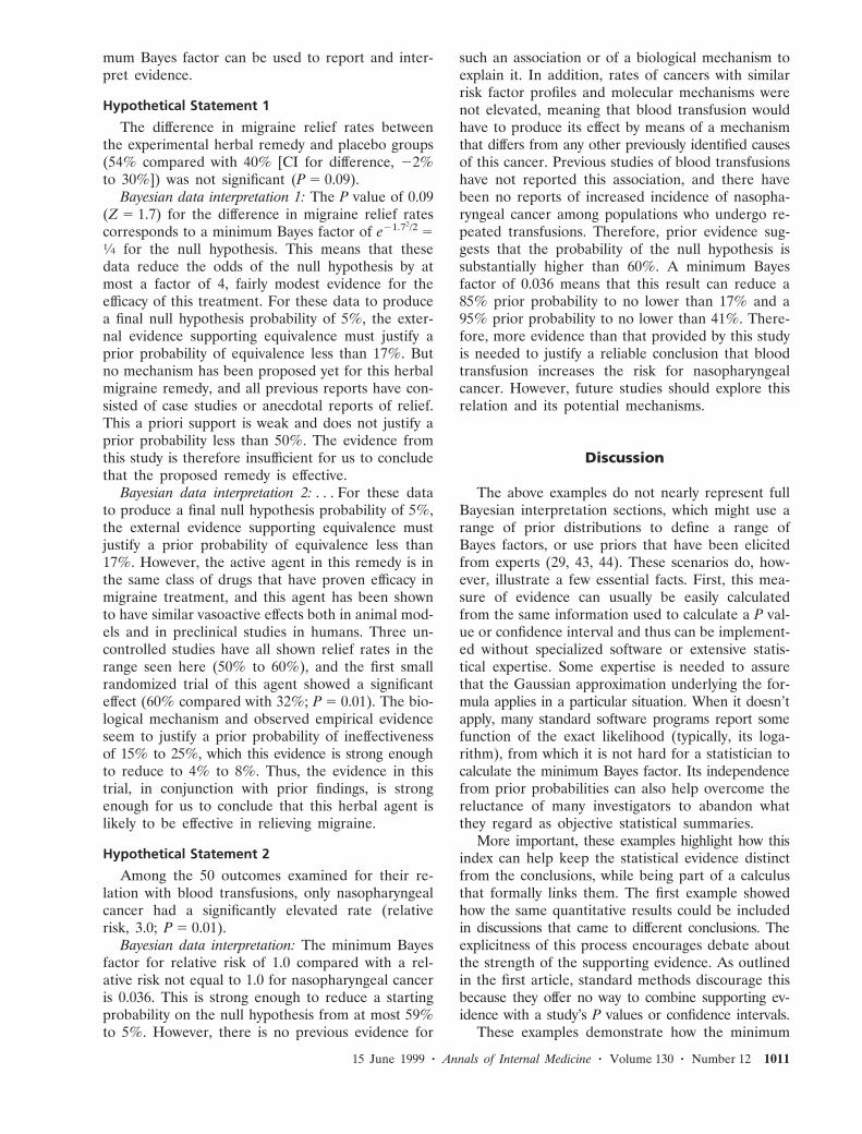
mum Bayes factor can be used to report and inter-pret evidence.

Hypothetical Statement 1

The difference in migraine relief rates betweenthe experimental herbal remedy and placebo groups(54% compared with 40% [CI for difference, 22%to 30%]) was not significant (P 5 0.09).

Bayesian data interpretation 1: The P value of 0.09(Z 5 1.7) for the difference in migraine relief ratescorresponds to a minimum Bayes factor of e21.72/2 51⁄4 for the null hypothesis. This means that thesedata reduce the odds of the null hypothesis by atmost a factor of 4, fairly modest evidence for theefficacy of this treatment. For these data to producea final null hypothesis probability of 5%, the exter-nal evidence supporting equivalence must justify aprior probability of equivalence less than 17%. Butno mechanism has been proposed yet for this herbalmigraine remedy, and all previous reports have con-sisted of case studies or anecdotal reports of relief.This a priori support is weak and does not justify aprior probability less than 50%. The evidence fromthis study is therefore insufficient for us to concludethat the proposed remedy is effective.

Bayesian data interpretation 2: . . . For these datato produce a final null hypothesis probability of 5%,the external evidence supporting equivalence mustjustify a prior probability of equivalence less than17%. However, the active agent in this remedy is inthe same class of drugs that have proven efficacy inmigraine treatment, and this agent has been shownto have similar vasoactive effects both in animal mod-els and in preclinical studies in humans. Three un-controlled studies have all shown relief rates in therange seen here (50% to 60%), and the first smallrandomized trial of this agent showed a significanteffect (60% compared with 32%; P 5 0.01). The bio-logical mechanism and observed empirical evidenceseem to justify a prior probability of ineffectivenessof 15% to 25%, which this evidence is strong enoughto reduce to 4% to 8%. Thus, the evidence in thistrial, in conjunction with prior findings, is strongenough for us to conclude that this herbal agent islikely to be effective in relieving migraine.

Hypothetical Statement 2

Among the 50 outcomes examined for their re-lation with blood transfusions, only nasopharyngealcancer had a significantly elevated rate (relativerisk, 3.0; P 5 0.01).

Bayesian data interpretation: The minimum Bayesfactor for relative risk of 1.0 compared with a rel-ative risk not equal to 1.0 for nasopharyngeal canceris 0.036. This is strong enough to reduce a startingprobability on the null hypothesis from at most 59%to 5%. However, there is no previous evidence for

such an association or of a biological mechanism toexplain it. In addition, rates of cancers with similarrisk factor profiles and molecular mechanisms werenot elevated, meaning that blood transfusion wouldhave to produce its effect by means of a mechanismthat differs from any other previously identified causesof this cancer. Previous studies of blood transfusionshave not reported this association, and there havebeen no reports of increased incidence of nasopha-ryngeal cancer among populations who undergo re-peated transfusions. Therefore, prior evidence sug-gests that the probability of the null hypothesis issubstantially higher than 60%. A minimum Bayesfactor of 0.036 means that this result can reduce a85% prior probability to no lower than 17% and a95% prior probability to no lower than 41%. There-fore, more evidence than that provided by this studyis needed to justify a reliable conclusion that bloodtransfusion increases the risk for nasopharyngealcancer. However, future studies should explore thisrelation and its potential mechanisms.

Discussion

The above examples do not nearly represent fullBayesian interpretation sections, which might use arange of prior distributions to define a range ofBayes factors, or use priors that have been elicitedfrom experts (29, 43, 44). These scenarios do, how-ever, illustrate a few essential facts. First, this mea-sure of evidence can usually be easily calculatedfrom the same information used to calculate a P val-ue or confidence interval and thus can be implement-ed without specialized software or extensive statis-tical expertise. Some expertise is needed to assurethat the Gaussian approximation underlying the for-mula applies in a particular situation. When it doesn’tapply, many standard software programs report somefunction of the exact likelihood (typically, its loga-rithm), from which it is not hard for a statistician tocalculate the minimum Bayes factor. Its independencefrom prior probabilities can also help overcome thereluctance of many investigators to abandon whatthey regard as objective statistical summaries.

More important, these examples highlight how thisindex can help keep the statistical evidence distinctfrom the conclusions, while being part of a calculusthat formally links them. The first example showedhow the same quantitative results could be includedin discussions that came to different conclusions. Theexplicitness of this process encourages debate aboutthe strength of the supporting evidence. As outlinedin the first article, standard methods discourage thisbecause they offer no way to combine supporting ev-idence with a study’s P values or confidence intervals.

These examples demonstrate how the minimum


Bayes factor enables simple threshold Bayesian anal-yses to be performed without a formal elicitation ofprior probability distributions. One merely has toargue that the prior probability of the null hypoth-esis is above or below a threshold value, on the ba-sis of the evidence from outside the study. If thestrongest evidence against the null hypothesis (theminimum Bayes factor) is not strong enough tosufficiently justify a conclusion, then the weaker evi-dence derived from a Bayes factor from a full Baye-sian analysis will not be either.

The use of the minimum Bayes factor does notpreclude a formal Bayesian analysis and indeed mightbe an entree to one. Recent reviews and booksoutline how full Bayesian analyses can be conductedand reported (21, 29, 45–50). Bayesian results canalso be extended into formal decision analyses (51).The availability of user-friendly software for Baye-sian calculations (52) makes implementation of thismethod more practicable now than in the past.

In not using a proper Bayesian prior probabilitydistribution, the minimum Bayes factor represents acompromise between Bayesian and frequentist per-spectives, which can be criticized from both camps.Some statisticians might deride the minimum Bayesfactor as nothing more than a relabelled P value.But as I have tried to show, P values and Bayesfactors are far more than just numbers, and movingto Bayes factors of any kind frees us from theflawed conceptual framework and improper view ofthe scientific method that travels with the P value.

The Bottom Line: Both Perspectives AreNecessary, but P Values Are Not

Standard frequentist methods are most problem-atic when used to draw conclusions in a single ex-periment. Their denial of a formal role for externalinformation in inference poses serious practical andlogical problems. But Bayesian methods, designedfor inductive inference in single experiments, do notguarantee that in the long run, conclusions in whichwe have 95% confidence will turn out to be true95% of the time (53). This is because Bayesianprior probability distributions are not ideal quantita-tive descriptors of what we know (or what we don’tknow) (54, 55), and Bayes theorem is an imperfectmodel for human learning (54, 56). This means thatthe frequentist, long-run perspective cannot be com-pletely ignored, leading many statisticians to empha-size the importance of using frequentist criteria in theevaluation of Bayesian and likelihood methods (6, 13,32, 53), which these methods typically fulfill quite well.

In the end, we must recognize that there is noautomatic method in statistics, as there is not in life,that allows us both to evaluate individual situations

and know exactly what the long-run consequencesof that evaluation will be. The connection betweeninference in individual experiments and the numberof errors we make over time is not found in the Pvalue or in hypothesis tests. It is found only inproperly assessing the strength of evidence from anexperiment with Bayes factors and uniting this witha synthesis of all of the other scientific informationthat bears on the question at hand. There is noformula for performing that synthesis, nor is there aformula for assigning a unique number to it. That iswhere room for meaningful scientific discourse lies.

Sir Francis Bacon, the writer and philosopherwho was one of the first inductivists, commented onthe two attitudes with which one can approach na-ture. His comment could apply to the perspectivescontrasted in these essays: “If we begin with cer-tainties, we shall end in doubts; but if we begin withdoubts, and are patient with them, we shall end withcertainties” (57). Putting P values aside, Bayesianand frequentist approaches each provide an essen-tial perspective that the other lacks. The way in whichwe balance their sometimes conflicting demands iswhat makes the process of learning from nature cre-ative, exciting, uncertain, and, most of all, human.

Appendix I

Derivation of the minimum Bayes factor under a Gauss-ian distribution: The likelihood of a hypothesis given an ob-served effect, x, is proportional to the probability of x underthat hypothesis. For a Gaussian distribution, the hypothe-sis typically concerns the mean. The probability of x undera Gaussian distribution with true mean 5 m and standarderror 5 s, is (where the symbol “u” is read as “given”):

Pr(xu m, s) 51

sÎ2pe

2Sx2m

sD2

Y2

Because the exponent is negative, the above probabil-ity is maximized when the exponent is zero, which occurswhen m 5 x (that is, the true mean m equals the observedeffect, x). The likelihood ratio for the null hypothesis (m 5 0)versus the maximally supported hypothesis (m 5 x) is theminimum Bayes factor:

Pr(xu m 5 0,s)Pr(xu m 5 x,s) 5

1sÎ2p

e2Sx20

sD2

Y2

1sÎ2p

e2Sx2x

sD

2

Y2

5 e2Sx

sD2

Y2

Because the Z-score is the observed effect, x, divided byits standard error, s, the final term in the above equation is:

e2Sx

sD2Y2 5 e2Z2/2


Appendix II

In the example posed in the first article (1), two treat-ments, called A and B, were compared in the same pa-tients, and the preferred treatment in each patients waschosen. The two experimenters had different mindsetswhile conducting the experiment: one planned to study allsix patients, whereas the other planned to stop as soon astreatment B was preferred. The first five patients pre-ferred treatment A, and the sixth preferred treatment B.

The probability of the data under the two hypothesesis as follows.

Null hypothesis: Probability that treatment A is pre-ferred 5 1/2

Alternative hypothesis: Probability that treatment A ispreferred 5 5/6

In the “n 5 6” experiment, this ratio is:

6S1

2D5S1

2D1Y6S5

6D5S1

6D1

5 0.23

The “6” appears above because the preference for treat-ment B could have occurred in any of the first five pa-tients or in the sixth patient without a change in theinference.

In the “stop at first preference for treatment B” ex-periment, the ratio is:

S1

2D5S1

2D1YS5

6D5S1

6D1

5 0.23

Acknowledgments: The author thanks Dan Heitjan, Russell Lo-calio, Harold Lehmann, and Michael Berkwitz for helpful com-ments on earlier versions of this article. The views expressed arethe sole responsibility of the author.

Requests for Reprints: Steven N. Goodman, MD, PhD, JohnsHopkins University, 550 North Broadway, Suite 409, Baltimore,MD 21205; e-mail, [email protected].

References

1. Goodman SN. Toward evidence-based medical statistics. 1: The P value fal-lacy. Ann Intern Med. 1999;130:995-1004.

2. Edwards A. A History of Likelihood. International Statistical Review. 1974;42:9-15.

3. Fisher LD. Comments on Bayesian and frequentist analysis and interpretationof clinical trials. Control Clin Trials. 1996;17:423-34.

4. Brophy JM, Joseph L. Placing trials in context using Bayesian analysis.GUSTO revisited by Reverend Bayes. JAMA. 1995;273:871-5.

5. Browne RH. Bayesian analysis and the GUSTO trial. Global Utilization ofStreptokinase and Tissue Plasminogen Activator in Occluded Coronary Arter-ies [Letter]. JAMA. 1995;274:873.

6. Good I. Probability and the Weighing of Evidence. New York: Charles Griffin;1950.

7. Cornfield J. The Bayesian outlook and its application. Biometrics. 1969;25:617-57.

8. Berger JO, Berry DA. Statistical analysis and the illusion of objectivity. Amer-ican Scientist. 1988;76:159-65.

9. Berry D. Interim analyses in clinical trials: classical vs. Bayesian approaches.Stat Med. 1985;4:521-6.

10. Belanger D, Moore M, Tannock I. How American oncologists treat breastcancer: an assessment of the influence of clinical trials. J Clin Oncol. 1991;9:7-16.

11. Omoigui NA, Silver MJ, Rybicki LA, Rosenthal M, Berdan LG, Pieper K,et al. Influence of a randomized clinical trial on practice by participatinginvestigators: lessons from the Coronary Angioplasty Versus Excisional Athe-rectomy Trial (CAVEAT). CAVEAT I and II Investigators. J Am Coll Cardiol.1998;31:265-72.

12. Goodman SN, Royall R. Evidence and scientific research. Am J PublicHealth. 1988;78:1568-74.

13. Royall R. Statistical Evidence: A Likelihood Primer. Monographs on Statisticsand Applied Probability, #71. London: Chapman and Hall; 1997.

14. Edwards A. Likelihood. Cambridge, UK: Cambridge Univ Pr; 1972.15. Goodman SN. Meta-analysis and evidence. Control Clin Trials. 1989;10:188-

204, 435.16. Efron B. Empirical Bayes methods for combining likelihoods. Journal of the

American Statistical Association. 1996;91:538-50.17. Hardy RJ, Thompson SG. A likelihood approach to meta-analysis with ran-

dom effects. Stat Med. 1996;15:619-29.18. Berger J. Statistical Decision Theory and Bayesian Analysis. New York: Springer-

Verlag; 1985.19. Edwards W, Lindman H, Savage L. Bayesian statistical inference for psy-

chological research. Psychol Rev. 1963;70:193-242.20. Diamond GA, Forrester JS. Clinical trials and statistical verdicts: probable

grounds for appeal. Ann Intern Med. 1983;98:385-94.21. Lilford R, Braunholtz D. The statistical basis of public policy: a paradigm

shift is overdue. BMJ. 1996;313:603-7.22. Peto R. Why do we need systematic overviews of randomized trials? Stat

Med. 1987;6:233-44.23. Pogue J, Yusuf S. Overcoming the limitations of current meta-analysis of

randomised controlled trials. Lancet. 1998;351:47-52.24. Fisher R. Statistical Methods and Scientific Inference. 3d ed. New York:

Macmillan; 1973.25. Jeffreys H. Theory of Probability. 2d ed. Oxford: Oxford Univ Pr; 1961.26. Kass R, Raftery A. Bayes Factors. Journal of the American Statistical Asso-

ciation. 1995;90:773-95.27. Cornfield J. A Bayesian test of some classical hypotheses—with applications

to sequential clinical trials. Journal of the American Statistical Association.1966;61:577-94.

28. Kass R, Greenhouse J. Comments on “Investigating therapies of potentiallygreat benefit: ECMO” (by JH Ware). Statistical Science. 1989;4:310-7.

29. Spiegelhalter D, Freedman L, Parmar M. Bayesian approaches to random-ized trials. Journal of the Royal Statistical Society, Series A. 1994;157:357- 87.

30. Berger J, Sellke T. Testing a point null hypothesis: the irreconcilability ofp-values and evidence. Journal of the American Statistical Association. 1987;82:112-39.

31. Bayarri M, Berger J. Quantifying surprise in the data and model verification.Proceedings of the 6th Valencia International Meeting on Bayesian Statistics,1998. 1998:1-18.

32. Carlin C, Louis T. Bayes and Empirical Bayes Methods for Data Analysis.London: Chapman and Hall; 1996.

33. Casella G, Berger R. Reconciling Bayesian and frequentist evidence in theone-sided testing problem. Journal of the American Statistical Association.1987;82:106-11.

34. Howard J. The 2 3 2 table: a discussion from a Bayesian viewpoint. Statis-tical Science. 1999;13:351-67.

35. Cornfield J. Sequential trials, sequential analysis and the likelihood principle.American Statistician. 1966;20:18-23.

36. Savitz DA, Olshan AF. Multiple comparisons and related issues in the in-terpretation of epidemiologic data. Am J Epidemiol. 1995;142:904-8.

37. Perneger T. What’s wrong with Bonferroni adjustments. BMJ. 1998;316:1236-8.

38. Goodman SN. Multiple comparisons, explained. Am J Epidemiol. 1998;147:807-12.

39 Thomas DC, Siemiatycki J, Dewar R, Robins J, Goldberg M, ArmstrongBG. The problem of multiple inference in studies designed to generate hy-potheses. Am J Epidemiol. 1985;122:1080-95.

40. Greenland S, Robins JM. Empirical-Bayes adjustments for multiple compar-isons are sometimes useful. Epidemiology. 1991;2:244-51.

41. Rothman KJ. No adjustments are needed for multiple comparisons. Epide-miology. 1990;11:43-6.

42. Berry DA. A case for Bayesianism in clinical trials. Stat Med. 1993;12:1377-93.43. Chaloner K, Church T, Louis T, Matts J. Graphical elicitation of a prior

distribution for a clinical trial. The Statistician. 1993;42:341-53.44. Chaloner K. Elicitation of prior distributions. In: Berry D, Stangl D, eds.

Bayesian Biostatistics. New York: Marcel Dekker; 1996.45. Freedman L. Bayesian statistical methods [Editorial]. BMJ. 1996;313:569-70.46. Fayers PM, Ashby D, Parmar MK. Tutorial in biostatistics: Bayesian data

monitoring in clinical trials. Stat Med. 1997;16:1413-30.47. Etzioni RD, Kadane JB. Bayesian statistical methods in public health and

medicine. Annu Rev Public Health. 1995;16:23-41.48. Berry DA. Benefits and risks of screening mammography for women in their

forties: a statistical appraisal. J Natl Cancer Inst. 1998;90:1431-9.49. Hughes MD. Reporting Bayesian analyses of clinical trials. Stat Med. 1993;

12:1651-64.50. Berry DA, Stangl D, eds. Bayesian Biostatistics. New York: Marcel Dekker;

1996.51. Berry DA. Decision analysis and Bayesian methods in clinical trials. Cancer

Treat Res. 1995;75:125-54.52. Spiegelhalter D, Thomas A, Best N, Gilks W. BUGS: Bayesian Inference

Using Gibbs Sampling. Cambridge, UK: MRC Biostatistics Unit; 1998. Avail-able at www.mrc-bsu.cam.ac.uk/bugs.

53. Rubin D. Bayesianly justifiable and relevant frequency calculations for theapplied statistician. Annals of Statistics. 1984;12:1151-72.

54. Shafer G. Savage revisited. Statistical Science. 1986;1:463-501.55. Walley P. Statistical Reasoning with Imprecise Probabilities. London: Chap-

man and Hall; 1991.56. Tversky A, Kahneman D. Judgment under uncertainty: heuristics and bi-

ases. In: Slovic P, Tversky A, Kahneman D, eds. Judgment under Uncertainty:Heuristics and Biases. Cambridge: Cambridge Univ Pr; 1982:1-20.

57. Bacon F. De Augmentis Scientarium, Book I (1605). In: Curtis C, Greenslet F,eds. The Practical Cogitator. Boston: Houghton Mifflin; 1962.


Standing Statistics Right Side Up

During the years I taught students about diag-nostic reasoning, I would begin by explaining

that the sensitivity of a diagnostic test for disease Xis found by measuring how often the test result ispositive in a population of patients, all of whom areknown (by some independent and definitive crite-rion, the “gold standard“) to have disease X: that is,by measuring the frequency of true-positive resultsin that population. A test that yields positive resultsin 95 of 100 diseased patients, for example, has asensitivity of 0.95. We would then talk about testspecificity—the likelihood that the same test wouldhave a false-positive result in a population of pa-tients known by the gold standard not to have thedisease. A test that yields positive results in 10 of100 nondiseased patients has a specificity of 0.90.

I would then ask the students to imagine that inworking up a new patient, they have gotten back apositive result from a test with the above sensitivityand specificity. What would they tell the patientabout his or her probability of having disease X?Their answer was almost always “95%.” On the faceof it, that answer seems pretty reasonable: Isn’t that

what you’d expect if a test were capable of detecting95% of diseased patients? The problem is, it’swrong; worse, it actually stands diagnostic reasoningon its head.

In fact, test sensitivity and specificity are deduc-tive measurements; they reason down from hypoth-esis (we assume the truth of the hypothesis that thepatient being tested does, or does not, have the dis-ease) to data (the likelihood that we will get apositive test result). The students’ reasoning is up-side down because what clinicians and patients re-ally need to know is exactly the inverse. In short,they need an inductive measurement, a reasoning upfrom data (the test result) to hypothesis (that thepatient has the disease).

Stated differently, what clinicians and patientsneed is a way to calculate the probability that anyparticular test result, positive or negative, is a trueresult. It is possible to make that inductive calcula-tion, but doing so requires combining sensitivity andspecificity to create something called a likelihoodratio, which is an overall measure of the “evidence”provided by the test result (positive or negative)itself. The likelihood ratio is then used to modifythe pretest estimate (the “prior probability”) thatThis paper is also available at http://www.acponline.org.


the patient has the disease, thereby creating a newand better post-test estimate—sometimes known asthe test’s predictive value—of the chance that thepatient has the disease. (For obvious reasons, pre-dictive values are also known as posterior probabili-ties. Positive predictive values express the post-testlikelihood that disease is present after a positive testresult; negative predictive values indicate the post-test likelihood that disease is absent after a negativetest result.)

Although the deductive inference in a test’s sen-sitivity and specificity differs profoundly from theinductive inference in its predictive values, that dif-ference is also an extremely subtle one; it was notwidely appreciated in the biomedical literature untilthe mid-1970s (1). In a two-part article in this issue(2, 3), Goodman demonstrates how the standardstatistical methods (sometimes called “frequentist”statistics) used in analyzing biomedical research,which we have come to accept as a kind of revealedtruth, also stand statistical inference on its head inmuch the same way that students’ initial attempts atdiagnostic reasoning do.

The article by Goodman is not light reading. Heis, however, a true hermeneut, a venerable wordmeaning “one who is skilled at interpretation.”Those who make the effort to understand him willbe rewarded with a number of important, if discon-certing, insights. Thus, just as clinicians need toknow the likelihood that a particular patient has adisease given a certain test result, researchers (andthose who read papers describing research) need toknow the likelihood that a hypothesis is true giventhe data actually obtained in a particular trial orexperiment. Both of these are inductive inferences.But, as Goodman points out, researchers generallyresort to an inverse, deductive calculation. That is,they calculate the probability of finding the resultsthey actually obtained, plus any more extreme re-sults, on the assumption that a certain hypothesis istrue (usually the “null hypothesis”—the assumptionthat the comparison groups do not differ), a conceptexpressed in the all-too-familiar P value.

The P value has been the subject of much criti-cism because a P value of 0.05 has been frequentlyand arbitrarily misused to distinguish a true effectfrom lack of effect. Although Goodman does notdisagree with that criticism, his real concerns liedeeper, and he catalogues for us several more seri-ous and more convoluted misinterpretations of theconcepts of evidence, error, and testing. These mis-conceptions are particularly troubling because theyconfuse our ability to judge whether, over the longrun of experience with many studies, “we shall notoften be wrong” with our ability to judge the like-lihood that each separate hypothesis tested in anindividual study is true or false.

Enter Bayes theorem. Unfortunately, those omi-nous words, with their associations of hazy priorprobabilities and abstruse mathematical formulas,strike fear into the hearts of most of us, clinician,researcher, and editor alike. But Bayesian inferenceimmediately loses much of its menace once we re-alize that it is, in fact, the exact equivalent of pre-dictive value, a concept now familiar from its wideuse in diagnostic reasoning. It also helps to under-stand that, mathematical niceties aside, Bayes theo-rem is essentially a quantitative description of whatwe do, qualitatively, every minute of the day: usenew information inductively to refine our judgmentsabout the correctness of what we already know. Infancier language, Bayesian inference says that themost effective way to develop a new and betterdegree of confidence (posterior odds) in our knowl-edge is to combine our previous confidence, derivedfrom sources outside a particular test or study (theprior odds), with the “evidence” from that test orstudy itself (the Bayes factor).

The importance of information from outsidesources becomes particularly clear in consideringthe impact of a single diagnostic test across the fullspectrum of clinical situations. Thus, the positivepredictive value (posterior probability of disease) ofeven a fairly sensitive and specific test might be only0.1 or 0.2 when that test is used in the “screeningmode,” that is, when the patient being tested is veryunlikely to have the disease in the first place. In thissituation, combining the “evidence”—the likelihoodratio for a positive test result—with outside infor-mation—a very low pretest (prior) probability—changes that probability relatively little, unless thespecificity of the test involved is almost perfect. Incontrast, the positive predictive value of the verysame test might be 0.90 to 0.95 or higher whentesting in the “confirmatory mode,” that is, whentesting is done in a patient who is already stronglysuspected of having the disease. Here, a relativelyhigh pretest (prior) probability can become substan-tially higher when it is combined with the evidencefrom a test that has even relatively modest specific-ity. The same test can produce intermediate positivepredictive values when testing is done in the “diag-nostic mode,” that is, when the pretest (prior) sus-picion of disease is moderate to begin with.

In like fashion, the use of prior knowledge iscritical in interpreting biomedical studies, and fail-ure to take it into account can easily lead to seriousmisinterpretation of the “evidence.” For example, arecent meta-analysis found an odds ratio of 1.66 infavor of the beneficial effects of homeopathic ther-apies over placebos. The associated 95% CI of 1.33to 2.08, taken by itself, was interpreted as evidencethat is “not compatible with the hypothesis that theclinical effects of homeopathy are due to placebo”


(4). If, however, that evidence is combined with theminimal plausibility (extremely low prior probabil-ity) that clinically meaningful biological activity canresult from small doses of pure water, even waterthat is shaken in a special way, the resulting poste-rior level (posterior probability) of confidence inbiological activity remains very low. Explanationsother than biological efficacy are thus likely to ac-count for the results actually observed (5). Con-versely, in view of the existing evidence that vitaminE may protect against coronary heart disease, thefinding, reported in this issue (6), that vitamin Eappears statistically not to prevent ischemic strokeshould be interpreted as ratcheting down the prob-ability of stroke prevention slightly, rather thanflatly ruling out the possibility of such activity.

Figuring out the best way to combine the evi-dence from a trial with prior information fromsources outside the trial is an important challenge.It is also a very difficult one, because we oftenweigh outside information subjectively. Goodmanhas therefore chosen to focus his discussion primar-ily on the less controversial and more objective coreof Bayesian inference: the measure of “the evi-dence” from a trial or study. This measure is ex-pressed by the Bayes factor, a metric already famil-iar to many readers in the form of the likelihoodratio, and one that, in itself, provides logically soundand statistically meaningful information (3). An im-portant lesson from this element of his discussion isthat the statistical evidence against a null hypothesisis usually weaker when the data are interpreted byusing the Bayes factor than when the same data areinterpreted by using the P value approach.

Convinced that inductive inference is both usefuland feasible in interpreting scientific studies, in 1997we began encouraging authors of manuscripts sub-mitted to Annals to include Bayesian interpretationof their results (7). Few have done so, probablyboth because frequentist methods are universallytaught, enshrined in statistical software, and expect-ed by biomedical journals and because researchersare generally not familiar with alternative methods.Researchers will be particularly interested in Good-man’s essay, therefore, because Bayesian principlescan contribute importantly to the design of biomed-

ical studies. These principles include the importanceof an exhaustive search of the existing, prior evidence,a step that is now often omitted (8), and calculationof a minimum Bayes factor from the data. But oth-ers stand to benefit as well from working their waythrough his analysis. This includes clinicians, whoare increasingly required to interpret the strength ofevidence from individual studies in making decisionsat the bedside, and medical reporters, who are quickto seize on the latest individual trial without con-sidering other available studies, thereby creating agreat deal of unnecessary confusion.

Frequentist statistics can serve a useful purpose,but their limitations are many and serious. Somemembers of the biostatistical community have there-fore worked long and hard to encourage the medi-cal researchers and readers to use the Bayesianapproach to statistical inference in the design andinterpretation of their studies. Goodman’s article isan elegant reflection of those efforts, providing bothan explication of underlying theory and solid sug-gestions for practice. In our view, this article willcontribute importantly to the task of standing sta-tistical inference right side up. We recommend it toour readers’ most serious attention.

Frank Davidoff, MDEditor

Ann Intern Med. 1999;130:1019-1021.

References

1. Galen RS, Gambino SR. Beyond Normality: The Predictive Value and Effi-ciency of Medical Diagnoses. New York: Wiley; 1975.

2. Goodman SN. Toward evidence-based medical statistics. 1: The P value fal-lacy. Ann Intern Med. 1999;130:995-1004.

3. Goodman SN. Toward evidence-based medical statistics. 2: The Bayes factor.Ann Intern Med. 1999;130:1005-13.

4. Linde K, Clausius N, Ramirez G, Melchart D, Eitel F, Hedges LV, et al.Are the clinical effects of homeopathy placebo effects? A meta-analysis ofplacebo-controlled trials. Lancet. 1997;350:834-43.

5. Vandenbroucke JP. 175th anniversary lecture. Medical journals and the shap-ing of medical knowledge. Lancet. 1998;352:2001-6.

6. Ascherio A, Rimm EB, Hernan MA, Giovannucci E, Kawachi I, StampferMJ, et al. Relation of consumption of vitamin E, vitamin C, and carotenoids torisk for stroke among men in the United States. Ann Intern Med. 1999;130:963-70.

7. Information for authors. Ann Intern Med. 1997;127:I-15.8. Clarke M, Chalmers I. Discussion sections in reports of controlled trials pub-

lished in general medical journals: islands in search of continents? JAMA.1998;280:280-2.

© 1999 American College of Physicians–American Society of InternalMedicine


Documents

Toward Evidence-Based Medical Statistics. 1: The P - PERFendo