Toward GIT stability of syzygies of canonical curves · Toward GIT stability of syzygies of canonical curves Anand Deopurkar, Maksym Fedorchuk and David Swinarski Abstract We introduce

Toward GIT stability of syzygies of canonical curves

Anand Deopurkar, Maksym Fedorchuk and David Swinarski

Abstract

We introduce the problem of GIT stability for syzygy points of canonical curves with aview toward a GIT construction of the canonical model of Mg. As the first step in thisdirection, we prove semi-stability of the 1st syzygy point for a general canonical curveof odd genus.

1. Introduction

By analogy with Hilbert points of Gieseker [Gie77, p.234], we introduce syzygy points of canonicalcurves and initiate the program of studying their GIT stability. The eventual goal of this programis a GIT construction of the canonical model of Mg, a problem whose origins lie in the log minimalmodel program for the moduli space of stable curves. Introduced by Hassett and Keel, the logMMP for Mg aims to construct certain log canonical models of Mg in a way that allows modularinterpretation [Has05]. The log canonical divisors on (the stack)Mg considered in this programare

KMg+ αδ = 13λ− (2− α)δ, for α ∈ [0, 1] ∩Q.

The work done so far suggests that we can construct some of these models as GIT quotientsof spaces of Hilbert points of n-canonically embedded curves. This is already evidenced in thework of Gieseker [Gie82] and Schubert [Sch91], who analyzed the cases of n > 5 and n = 3,respectively. Recent work of Hassett and Hyeon [HH09, HH13] extends the GIT analysis ton = 2 and constructs the first two log canonical models of Mg corresponding to α > 2

3 ; see also[AFSvdW13]. Subsequent work along this direction suggests that the case of n = 1 and the useof finite Hilbert points would yield log canonical models corresponding to the values of α downto α = g+6

7g+6 [AFS13, FJ12].

The ultimate goal of the Hassett–Keel program is to reach α = 0, which corresponds to thecanonical model of Mg. To go beyond α = g+6

7g+6 and indeed down to α = 0, Farkas and Keel

suggested that one should construct birational models of Mg as GIT quotients using syzygies ofcanonically embedded curves. In this paper, we make the first step toward this goal by provinga generic semi-stability result for the 1st syzygies in odd genus.

Main Theorem. A general canonical curve of odd genus g > 5 has a semi-stable 1st syzygypoint.

2010 Mathematics Subject Classification 14L24, 13D02, 14H10Keywords: canonical curves, syzygies, Geometric Invariant Theory, ribbons

M.F. is supported by the NSF grant DMS-1259226.

http://www.ams.org/msc/


Our strategy for proving generic semi-stability of syzygy points follows that of [AFS13] forproving generic semi-stability of finite Hilbert points. Namely, we prove the semi-stability of the1st syzygy point of a singular curve with Gm-action — the balanced ribbon — by a method of[MS11].

Ribbons and the problem of studying syzygies of their canonical embeddings were originallyintroduced by Bayer and Eisenbud in [BE95]. Their motivation for studying ribbons was in thecontext of Green’s conjecture for smooth canonical curves. Namely, Bayer and Eisenbud askedwhether rational ribbons satisfy an appropriate version of Green’s conjecture [BE95, p.720].Although this question remains open in its full generality, an affirmative answer to it implies thegeneric Green’s conjecture, which is known thanks to the work of Voisin [Voi02, Voi05]. Green’sconjecture makes an appearance in the study of GIT stability of syzygies of canonical curves bycontrolling which syzygy points are well-defined, see Remark 2.4.

Outline of the paper.

In Section 2, we define syzygy points of a canonically embedded Gorenstein curve and give a pre-cise statement of our main result. In Section 3, we recall some preliminary results about balancedribbons. In the most technical Section 4, we construct several monomial bases of cosyzygies forthe balanced ribbon. Finally, in Section 5, we prove the main theorem by deducing semi-stabilityof the 1st syzygy point of the balanced ribbon from the existence of the monomial bases con-structed in Section 4.

Acknowledgements.

We learned the details of Farkas and Keel’s idea to use syzygies as the means to construct thecanonical model of Mg from a talk given by Gavril Farkas at the AIM workshop Log minimalmodel program for moduli spaces held in December 2012. This paper grew out of our attemptto implement the roadmap laid out in that talk. We are grateful to AIM for the opportunity tomeet. The workshop participants of the working group on syzygies, among them David Jensen,Ian Morrison, Anand Patel, and the present authors, verified by a computer computation ourmain result for g = 7. This computation motivated us to search for a proof in the general case.

2. Syzygy points of canonical curves

In this section, we recall some basic notions of Koszul cohomology and set-up the GIT problemsfor the linear syzygies of a canonical curve. We refer to [Gre84] and [AF11b] for a completetreatment of Koszul cohomology and a detailed discussion of Green’s conjecture.

We define a canonical Gorenstein curve to be a Gorenstein curve C with a very ampledualizing sheaf ωC . The arithmetic genus of such C is at least 3. In this paper, we are exclusivelyconcerned with Koszul cohomology of the pair (C,ωC). Namely, associated to C and the linebundle ωC is the Koszul complex

p+1∧H0(ωC)⊗H0(ωq−1C )

fp+1,q−1−−−−−−→p∧

H0(ωC)⊗H0(ωqC)fp,q−−−−−−→

p−1∧H0(ωC)⊗H0(ωq+1

C ) (1)

where the differential fp,q is given by

fp,q(x0 ∧ x1 ∧ · · · ∧ xp−1 ⊗ y) =

p−1∑i=0

(−1)ix0 ∧ · · · ∧ xi ∧ · · · ∧ xp−1 ⊗ xiy.

2


The Koszul cohomology groups of (C,ωC) are

Kp,q(C) := ker fp,q/

im fp+1,q−1. (2)

We say that C satisfies property (Np) if Ki,q(C) = 0 for all (i, q) with i 6 p and q > 2. Inparticular, property (N0) means that the natural maps Symm H0(ωC) → H0(ωmC ) are surjectivefor all m, i.e., that C is projectively normal in its canonical embedding. Property (Np) for p > 1means, in addition, that the ideal of C in the canonical embedding is generated by quadrics andthe syzygies of order up to p are linear.

Remark 2.1 (On projective normality of canonical Gorenstein curves). A classical theorem ofMax Noether says that a smooth curve C of genus g > 3 is non-hyperelliptic if and only if ωC isvery ample if and only if C satisfies property (N0) [ACGH85, p.117]. A relatively recent result[KM09] extends these equivalences to the case when C is an integral Gorenstein curve. We are notaware of a general result concerning projective normality of non-integral Gorenstein curves. Inparticular, it appears that the case of reducible curves is open in general [BB11]. Because of thisand because our primary object of study is a non-reduced curve (namely, a rational ribbon), weoften specify projective normality as a hypothesis. We do note that projective normality of non-hyperelliptic ribbons is established in the original paper of Bayer and Eisenbud [BE95, Theorem5.3]. An explicit proof for the case of the balanced ribbon appears in [AFS13, Proposition 3.5].

For p 6 g − 2, set

Γp(C) :=

(p+1∧

H0(ωC)⊗H0(ωC)

)/ p+2∧H0(ωC). (3)

The first four terms of the Koszul complex (1) in degree p+ 2 give the exact sequence

0→ Kp+1,1(C)→ Γp(C)→ ker fp,2 → Kp,2(C)→ 0.

We can thus readily compute that

dim ker fp,2 = (3g − 2p− 3)

(g − 1

p

), and

dim Γp(C) = g

(g

p+ 1

)−(

g

p+ 2

).

(4)

Definition 2.2. We define the space of pth order linear syzygies of C as the subspace of Γp(C)given by

Syzp(C) := Kp+1,1(C).

Suppose C satisfies property (Np) so that Kp,2(C) = 0. We define the space of pth order linearcosyzygies of C as the quotient space of Γp(C) given by

CoSyzp(C) := ker fp,2.

The relation of the above definition to the definition of syzygies in terms of the homogeneousideal of C is as follows. Let

Im(C) = ker(Symm H0(ωC)→ H0(ωmC )

)be the degree m graded piece of the homogeneous ideal of C. Then the space of pth order linearsyzygies among the defining quadrics of C is taken to be the kernel of the map

p∧H0(ωC)⊗ I2(C)

α−→p−1∧

H0(ωC)⊗ I3(C).

3


A simple diagram chase now gives a well-known isomorphism kerα ' Kp+1,1(C).

Definition 2.3. Suppose C satisfies property (Np). We define the pth syzygy point of C to bethe quotient of Γp(C) given by [

Γp(C)→ CoSyzp(C)→ 0],

and interpreted as a point in the Grassmannian Grass(

(3g − 2p− 3)(g−1p

),Γp(C)

).

Abusing notation, we use CoSyzp(C) to denote both the vector space itself and the point in

Grass(

(3g − 2p− 3)(g−1p

),Γp(C)

)that it represents. Observe that the 0th syzygy point is simply

the 2nd Hilbert point.

Remark 2.4. For which curves is the pth syzygy point defined? According to a celebrated Green’sconjecture, a smooth canonical curve C satisfies (Np) if and only if p is less than the Cliffordindex of C. Formulated by Green in [Gre84], this conjecture remains open in its full generality.It is known to be true, however, for a large class of curves. Voisin proved that general canonicalcurves on K3 surfaces satisfy Green’s conjecture [Voi02, Voi05]. More recently, Aprodu andFarkas proved the conjecture for all smooth curves on K3 surfaces [AF11a]. In particular, thepth syzygy point of a generic curve of genus g is defined for all p < bg/2c.

Definition 2.5. We define Syzp to be the closure in Grass(

(3g − 2p− 3)(g−1p

),Γp(C)

)of the

locus of pth syzygy points of canonical curves satisfying property (Np).

Consider the group SLg ' SL(H0(ωC)). Its natural action on H0(ωC) induces actions on

the vector space Γp(C), the Grassmannian Grass(

(3g − 2p− 3)(g−1p

),Γp(C)

), and finally on

the subvariety Syzp. The Plucker line bundle on the Grassmannian comes with a natural SLglinearization, and so does its restriction to Syzp. A candidate for the pth syzygy model of Mg isthus the GIT quotient

Syzp// SLg .

Our main theorem shows that this quotient is non-empty for p = 1 and odd g > 5.

Theorem 2.6. A general canonical curve of odd genus g > 5 has a semi-stable 1st syzygy point.

We prove this theorem in Section 5; see Corollary 5.5.

3. The balanced canonical ribbon

We prove Theorem 2.6 by explicitly writing down a semi-stable point in Syz1. This point cor-responds to the syzygies of the balanced ribbon. Our exposition of its properties closely follows[AFS13] where the semi-stability of Hilbert points of this ribbon was established. Nevertheless,we recall the necessary details for the reader’s convenience.

Let g = 2k + 1. The balanced ribbon of genus g is the scheme R obtained by identifyingU := SpecC[u, ε]/(ε2) and V := SpecC[v, η]/(η2) along U \ 0 and V \ 0 via the isomorphism

u 7→ v−1 − v−k−2η,ε 7→ v−g−1η.

(5)

4


The scheme R is an example of a rational ribbon. While our proofs use only the balanced ribbon,we refer the reader to [BE95] for a more extensive study of ribbons in general.

Being a Gorenstein curve, R has a dualizing line bundle ω, generated by du∧dεε2

on U , and

by dv∧dηη2

on V . Since ω is very ample by [AFS13, Lemma 3.2], the global sections of ω embed

R as an arithmetically Gorenstein curve in Pg−1 by [BE95, Theorem 5.3]. As a result, we haveKp,q(R) = 0 for all q > 3 and p 6 g − 3. In particular, for all p < bg/2c, property (Np) isequivalent to Kp,2(R) = 0 [Ein87].

The balanced ribbon R admits a Gm-action, given by

t · u 7→ tu, t · ε 7→ tk+1ε ,

t · v 7→ t−1v, t · η 7→ t−k−1η.(6)

This action induces Gm-actions on H0(R,ωm) for all m. The next two propositions describe thesespaces along with their decomposition into weight spaces.

Proposition 3.1. A basis for H0(R,ω) is given by x0, . . . , x2k, where the xi’s restricted to Uare given by

xi =

ui du∧dε

ε2if 0 6 i 6 k(

ui + (i− k)ui−k−1ε)

du∧dεε2

if k < i 6 2k,

and where xi is a Gm-semi-invariant of weight i − k. In particular, H0(R,ω) splits as a directsum of g distinct Gm weight-spaces of weights −k, . . . , k.

Proof. That xi’s form a basis follows from [BE95, Theorem 5.1]. The statement about the weightsis obvious.

Remark 3.2 (Z2-symmetry). Observe that R has a Z2-symmetry given by the isomorphismV ' U defined by u ↔ v and ε ↔ η and commuting with the gluing isomorphism (5). TheZ2-symmetry exchanges xi and x2k−i.

The following observation from [AFS13, Lemma 3.4] deals with higher powers of ω:

Lemma 3.3 (Ribbon Product Lemma). Let 0 6 i1, . . . , im 6 2k be such that i1, . . . , i` 6 k andi`+1, . . . , im > k. On U , we have

xi1 · · ·xim =(ua + (a− b)ua−k−1ε

) (du ∧ dεε2

)m,

where

a = i1 + · · ·+ im ,

b = i1 + · · ·+ i` + k(m− `).

Definition 3.4. The u-weight (or u-degree) of a monomial xi1 · · ·xim is the sum i1 + · · ·+ im.Note that the u-weight of xi1 · · ·xim equals to the Gm-weight of xi1 · · ·xim plus km.

Proposition 3.5. Let m > 2. Let H0(R,ωm)d be the weight-space of H0(R,ωm) of u-weight d.Then

dim H0(R,ωm)d =

1 if 0 6 d 6 k,

2 if k < d < 2km− k,1 if 2km− k 6 d 6 2km.

Moreover, the map Symm H0(R,ω)→ H0(R,ωm) is surjective.

5


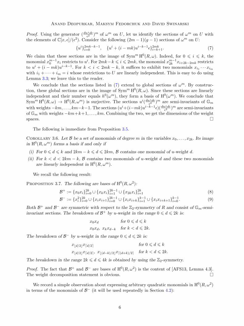
Proof. Using the generator (du∧dεε2

)m of ωm on U , let us identify the sections of ωm on U withthe elements of C[x, ε]/(ε2). Consider the following (2m− 1)(g − 1) sections of ωm on U :

ui2mk−k−1i=0 , ui + (i−mk)ui−k−1ε2mki=k+1. (7)

We claim that these sections are in the image of Symm H0(R,ω). Indeed, for 0 6 i 6 k, themonomial xm−10 xi restricts to ui. For 2mk−k 6 i 6 2mk, the monomial xm−12k xi+2k−2mk restrictsto ui + (i − mk)ui−k−1. For k < i < 2mk − k, it suffices to exhibit two monomials xi1 · · ·ximwith i1 + · · ·+ im = i whose restrictions to U are linearly independent. This is easy to do usingLemma 3.3; we leave this to the reader.

We conclude that the sections listed in (7) extend to global sections of ωm. By construc-tion, these global sections are in the image of Symm H0(R,ω). Since these sections are linearlyindependent and their number equals h0(ωm), they form a basis of H0(ωm). We conclude thatSymm H0(R,ω) → H0(R,ωm) is surjective. The sections ui(du∧dε

ε2)m are semi-invariants of Gm

with weights −km, . . . , km−k−1. The sections (ui+(i−mk)ui−k−1ε)(du∧dεε2

)m are semi-invariantsof Gm with weights −km+k+1, . . . , km. Combining the two, we get the dimensions of the weightspaces.

The following is immediate from Proposition 3.5.

Corollary 3.6. Let B be a set of monomials of degree m in the variables x0, . . . , x2k. Its imagein H0(R,ωm) forms a basis if and only if

(i) For 0 6 d 6 k and 2km− k 6 d 6 2km, B contains one monomial of u-weight d.

(ii) For k < d < 2km − k, B contains two monomials of u-weight d and these two monomialsare linearly independent in H0(R,ωm).

We recall the following result:

Proposition 3.7. The following are bases of H0(R,ω2):

B+ := x0xi2ki=0 ∪ xkxi2k−1i=1 ∪ x2kxi2ki=1 (8)

B− := x2i 2ki=0 ∪ xixi+12k−1i=0 ∪ xixi+kk−1i=1 ∪ xixi+k+1k−1i=0 . (9)

Both B+ and B− are symmetric with respect to the Z2-symmetry of R and consist of Gm-semi-invariant sections. The breakdown of B+ by u-weight in the range 0 6 d 6 2k is:

x0xd for 0 6 d 6 k

x0xd, xkxd−k for k < d 6 2k.

The breakdown of B− by u-weight in the range 0 6 d 6 2k is:

xbd/2cxdd/2e for 0 6 d 6 k

xbd/2cxdd/2e, xb(d−k)/2cxd(d+k)/2e for k < d 6 2k.

The breakdown in the range 2k 6 d 6 4k is obtained by using the Z2-symmetry.

Proof. The fact that B+ and B− are bases of H0(R,ω2) is the content of [AFS13, Lemma 4.3].The weight decomposition statement is obvious.

We record a simple observation about expressing arbitrary quadratic monomials in H0(R,ω2)in terms of the monomials of B− (it will be used repeatedly in Section 4.2):

6


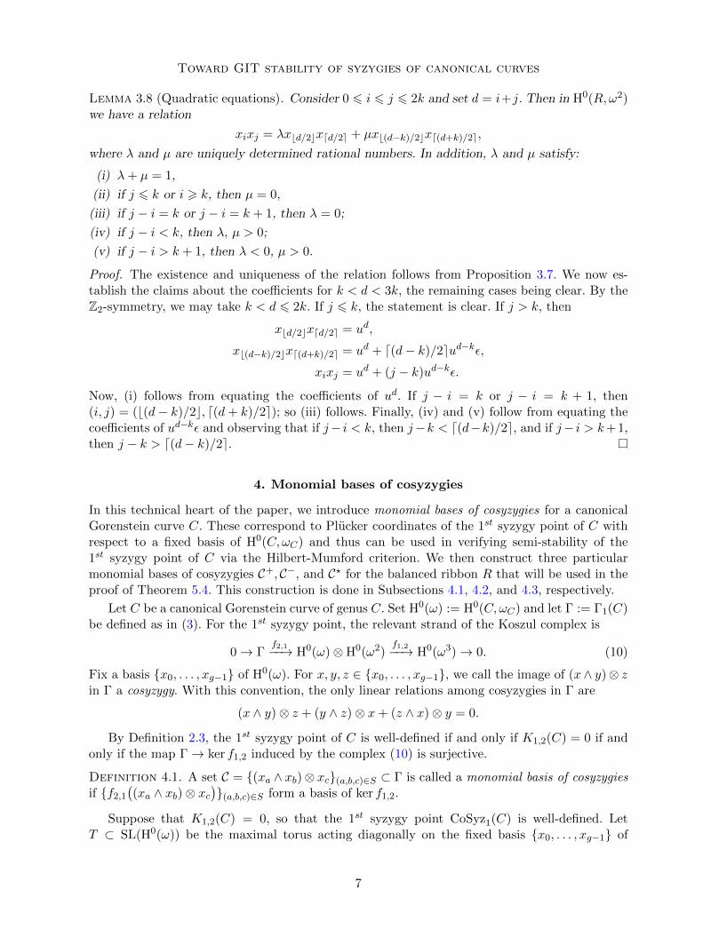
Lemma 3.8 (Quadratic equations). Consider 0 6 i 6 j 6 2k and set d = i+j. Then in H0(R,ω2)we have a relation

xixj = λxbd/2cxdd/2e + µxb(d−k)/2cxd(d+k)/2e,

where λ and µ are uniquely determined rational numbers. In addition, λ and µ satisfy:

(i) λ+ µ = 1,

(ii) if j 6 k or i > k, then µ = 0,

(iii) if j − i = k or j − i = k + 1, then λ = 0;

(iv) if j − i < k, then λ, µ > 0;

(v) if j − i > k + 1, then λ < 0, µ > 0.

Proof. The existence and uniqueness of the relation follows from Proposition 3.7. We now es-tablish the claims about the coefficients for k < d < 3k, the remaining cases being clear. By theZ2-symmetry, we may take k < d 6 2k. If j 6 k, the statement is clear. If j > k, then

xbd/2cxdd/2e = ud,

xb(d−k)/2cxd(d+k)/2e = ud + d(d− k)/2eud−kε,xixj = ud + (j − k)ud−kε.

Now, (i) follows from equating the coefficients of ud. If j − i = k or j − i = k + 1, then(i, j) = (b(d− k)/2c, d(d+ k)/2e); so (iii) follows. Finally, (iv) and (v) follow from equating thecoefficients of ud−kε and observing that if j− i < k, then j−k < d(d−k)/2e, and if j− i > k+1,then j − k > d(d− k)/2e.

4. Monomial bases of cosyzygies

In this technical heart of the paper, we introduce monomial bases of cosyzygies for a canonicalGorenstein curve C. These correspond to Plucker coordinates of the 1st syzygy point of C withrespect to a fixed basis of H0(C,ωC) and thus can be used in verifying semi-stability of the1st syzygy point of C via the Hilbert-Mumford criterion. We then construct three particularmonomial bases of cosyzygies C+, C−, and C? for the balanced ribbon R that will be used in theproof of Theorem 5.4. This construction is done in Subsections 4.1, 4.2, and 4.3, respectively.

Let C be a canonical Gorenstein curve of genus C. Set H0(ω) := H0(C,ωC) and let Γ := Γ1(C)be defined as in (3). For the 1st syzygy point, the relevant strand of the Koszul complex is

0→ Γf2,1−−→ H0(ω)⊗H0(ω2)

f1,2−−→ H0(ω3)→ 0. (10)

Fix a basis x0, . . . , xg−1 of H0(ω). For x, y, z ∈ x0, . . . , xg−1, we call the image of (x∧ y)⊗ zin Γ a cosyzygy. With this convention, the only linear relations among cosyzygies in Γ are

(x ∧ y)⊗ z + (y ∧ z)⊗ x+ (z ∧ x)⊗ y = 0.

By Definition 2.3, the 1st syzygy point of C is well-defined if and only if K1,2(C) = 0 if andonly if the map Γ→ ker f1,2 induced by the complex (10) is surjective.

Definition 4.1. A set C = (xa ∧ xb)⊗ xc(a,b,c)∈S ⊂ Γ is called a monomial basis of cosyzygiesif f2,1

((xa ∧ xb)⊗ xc

)(a,b,c)∈S form a basis of ker f1,2.

Suppose that K1,2(C) = 0, so that the 1st syzygy point CoSyz1(C) is well-defined. LetT ⊂ SL(H0(ω)) be the maximal torus acting diagonally on the fixed basis x0, . . . , xg−1 of

7


H0(ω). We obtain a distinguished basis of Γ consisting of the T -eigenvectors (xa∧xb)⊗xc. Thenthe monomial bases of cosyzygies of C correspond precisely to the non-zero Plucker coordinatesof CoSyz1(C) ∈ Grass ((3g − 5)(g − 1),Γ) with respect to this basis of eigenvectors in Γ. To everysuch coordinate, and in turn, to every monomial basis C, we can associate a T -character, calledthe T -state of C. We may represent the T -state as a linear combination of x0, . . . , xg−1. Precisely,the T -state of C = (xa ∧ xb)⊗ xc(a,b,c)∈S is given by

wT (C) :=∑

(a,b,c)∈S

wT((xa ∧ xb)⊗ xc

)=

∑(a,b,c)∈S

(xa + xb + xc) = n0x0 + · · ·+ ng−1xg−1,

where ni is the number of occurrences of xi among the cosyzygies in C. Note that we always have

g−1∑i=0

ni = 3(3g − 5)(g − 1).

Remark 4.2. Recall from Equation (4) that

dim ker f1,2 = (3g − 5)(g − 1).

Therefore, a set C = (xa ∧ xb)⊗ xc(a,b,c)∈S ⊂ Γ is a monomial basis of cosyzygies if and only ifthe following two conditions are satisfied

(i) C has (3g − 5)(g − 1) elements,

(ii)f2,1((xa ∧ xb)⊗ xc

)= xb ⊗ xaxc − xa ⊗ xbxc

(a,b,c)∈S span ker f1,2.

From now on, we assume that C = R is the balanced ribbon of genus g = 2k + 1 andx0, . . . , x2k is the basis of H0(ω) described in Proposition 3.1. Our goal for the rest of thissection is to construct three monomial bases of cosyzygies for R that will be used in Section 5to establish semi-stability of CoSyz1(R).

Notation: The following terminology will be in force throughout the rest of the paper. Wedefine the u-degree of a cosyzygy (xa ∧ xb) ⊗ xc ∈ Γ to be a + b + c and define the level of atensor xa ⊗ xbxc ∈ H0(ω) ⊗ H0(ω2) to be a. To lighten notation, we often use (xa ∧ xb) ⊗ xc todenote f2,1

((xa ∧ xb)⊗ xc

)= xb ⊗ xaxc − xa ⊗ xbxc in H0(ω)⊗H0(ω2).

For α ∈ Q, set α =⌊α+ 1

2

⌋. In other words, α is the integer closest to α. Observe that

for n ∈ Z, we have

n = bn/3c+ n/3+ dn/3e.We use 〈S〉 to denote the linear span of elements in a subset S of a vector space.

Outline of the construction: We first describe our strategy for constructing monomial basesof cosyzygies for the balanced ribbon R. From Definition 4.1, a set C = (xa∧xb)⊗xc(a,b,c)∈S ⊂Γ of (3g − 5)(g − 1) cosyzygies is a monomial basis of cosyzygies if and only if the imagesf2,1((xa ∧ xb)⊗ xc

), for (a, b, c) ∈ S, span ker f1,2. The first step in our construction is to write

down a set C of (3g − 5)(g − 1) cosyzygies. We do this heuristically.

Next, we make the following observation. Since im f2,1 ⊆ ker f1,2 and f1,2 is surjective ontoH0(ω3), to prove that the images of the cosyzygies in C span ker f1,2, it suffices to show that

dim(H0(ω)⊗H0(ω2)

) /〈f2,1((xa ∧ xb)⊗ xc)〉(a,b,c)∈S 6 dim H0(ω3) = 5(g − 1).

8


In order to do this, we treat

f2,1((xa ∧ xb)⊗ xc

)= xb ⊗ xaxc − xa ⊗ xbxc

as a relation among the elements of H0(ω) ⊗ H0(ω2). We therefore reduce to showing that therelations imposed by C reduce the dimension of H0(ω)⊗H0(ω2) to at most 5(g − 1).

The final observation is that all of our results and constructions respect the Gm-action on Rdescribed in Equation (6). In particular, we can run our argument by u-degree. This observationgreatly simplifies our task because the relevant weight spaces have small dimensions. In particular,by Proposition 3.5 we have

dim H0(ω3)d =

1 if 0 6 d 6 k or 5k 6 d 6 6k,

2 if k < d < 5k.(11)

4.1 A construction of the first monomial basis

We define C+ to be the union of the following sets of cosyzygies:

(T1) (x0 ∧ xi)⊗ xj , where i 6= 0, 2k and j 6= 2k.

(T2) (x0 ∧ xi)⊗ x2k, where 1 6 i 6 k − 1.

(T3) (x0 ∧ x2k)⊗ xi, where i 6 k − 1.

(T4) (x2k ∧ xi)⊗ xj , where i 6= 0, 2k and j 6= 0.

(T5) (x2k ∧ x0)⊗ xi, i > k + 1.

(T6) (x2k ∧ xi)⊗ x0, k + 1 6 i 6 2k − 1.

(T7) (xk ∧ xi)⊗ xj , where i 6= 0, k, 2k and j 6= 0, 2k.

(T8) (xk ∧ x0)⊗ x2k and (xk ∧ x2k)⊗ x0.(T9) (xi ∧ xk+i)⊗ xk−i where 1 6 i 6 k − 1.

(T10) (x2k−i ∧ xk−i)⊗ xk+i, 1 6 i 6 k − 1

Proposition 4.3. C+ is a monomial basis of cosyzygies for R with T -state

wT (C+) = (g2 − 1)(x0 + xk + x2k) + (6g − 6)∑

i 6=0,k,2k

xi.

Proof. Notice that C+ contains precisely (3g−5)(g−1) cosyzygies and that it is invariant underthe Z2-involution of the ribbon described in Remark 3.2.

To calculate the T -state of C+, observe that x0, xk, x2k each appear g2− 1 times, and xi, forevery i 6= 0, k, 2k, appears 6g − 6 times. It follows that

wT (C+) = (g2 − 1)(x0 + xk + x2k) + (6g − 6)∑

i 6=0,k,2k

xi.

We now verify that C+ is a monomial basis of cosyzygies. In view of the Z2-symmetry andthe dimensions of H0(ω3)d from (11), we only need to verify that the quotient space

(H0(ω) ⊗

H0(ω2))d/〈C+〉d is at most one-dimensional in u-degrees 0 6 d 6 k − 1, and at most two-

dimensional in u-degrees k 6 d 6 3k.

The key player in our argument is the monomial basis B+ from Proposition 3.7:

B+ =x0xi2ki=0, xkxi2k−1i=1 , x2kxi2ki=1

. (12)

9


Tensoring B+ with the standard basis x0, . . . , x2k of H0(ω), we obtain the following basis ofH0(ω)⊗H0(ω2):

B := xa ⊗m : 0 6 a 6 2k,m ∈ B+Our argument now proceeds by u-degree:

Degree 0 6 d 6 k. We have 〈B〉d = 〈xa ⊗ x0xd−a : where 0 6 a 6 d〉. Evidently, we havexaxd−a = x0xd in H0(ω2). It follows that

xa ⊗ x0xd−a = x0 ⊗ xaxd−a + (x0 ∧ xa)⊗ xd−a = x0 ⊗ x0xd + (x0 ∧ xa)⊗ xd−a,

where (x0∧xa)⊗xd−a is a cosyzygy (T1). We conclude that 〈B〉d/〈C+〉d is spanned by x0⊗x0xd,hence is at most one-dimensional.

Degree k + 1 6 d 6 2k. We have

〈B〉d = 〈xa ⊗ x0xd−a, xb ⊗ xkxd−k−b : 0 6 a 6 d, 0 6 b < d− k〉.

If b > 1, using the cosyzygies (T7) and (T1) and Lemma 3.8, we obtain

xb ⊗ xkxd−k−b = xk ⊗ xbxd−k−b + (xk ∧ xb)⊗ xd−k−b= xk ⊗ x0xd−k + (xk ∧ xb)⊗ xd−k−b= x0 ⊗ xkxd−k + (x0 ∧ xk)⊗ xd−k + (xk ∧ xb)⊗ xd−k−b.

Using (T1), we also have

xa ⊗ x0xd−a = x0 ⊗ xaxd−a + (x0 ∧ xa)⊗ xd−a,

It follows that 〈B〉d/〈C+〉d = 〈x0⊗xaxd−a : 0 6 a 6 d〉/〈C+〉d. In other words, every tensor of u-degree d is reduced to a tensor of level 0. Since dim〈x0⊗xaxd−a : 0 6 a 6 d〉 = dim H0(ω2)d = 2,we are done.

Degree 2k + 1 6 d 6 3k − 1. Write d = 2k + i, 1 6 i 6 k − 1. It is easy to see that moduloC+, every tensor in

(H0(ω)⊗ H0(ω2)

)d

can be reduced to a tensor of level 0, k, or 2k, by usingcosyzygies (T1)–(T4) or (T7). In other words,

〈B〉d/〈C+〉d = 〈x0 ⊗ xkxk+i, x0 ⊗ x2kxi, xk ⊗ x0xk+i, xk ⊗ xkxi, x2k ⊗ x0xi〉/〈C+〉d.

Since dim〈xi ⊗ xax2k−a : 0 6 a 6 2k〉 = dim H0(ω2)2k = 2, it suffices to show that everytensor in the above display can be rewritten modulo C+ as a tensor of level i. First, we observethat

x2k ⊗ x0xi = x0 ⊗ x2kxi + (x0 ∧ x2k)⊗ xi (using (T5) cosyzygy),

x0 ⊗ xix2k = xi ⊗ x0x2k − (x0 ∧ xi)⊗ x2k (using (T2) cosyzygy),

xk ⊗ xixk = xi ⊗ x2k − (xk ∧ xi)⊗ xk (using (T7) cosyzygy).

Since xk ⊗ x0xk+i = x0 ⊗ xkxk+i + (x0 ∧ xk)⊗ xk+i, it remains to show that x0 ⊗ xkxk+i can berewritten as a tensor of level i. To this end, we compute

x0 ⊗ xkxk+i = xk+i ⊗ x0xk − (x0 ∧ xk+i)⊗ xk = xk+i ⊗ xixk−i − (x0 ∧ xk+i)⊗ xk= xi ⊗ xk+ixk−i + (xi ∧ xk+i)⊗ xk−i − (x0 ∧ xk+i)⊗ xk,

where we have used a cosyzygy (T9) in the second line.

10


Degree d = 3k. Using cosyzygies (T1), (T4), and (T7), every tensor in 〈B〉3k reduces to atensor of level 0, k, or 2k. It follows that

〈B〉3k/〈C+〉3k = 〈x0 ⊗ xkx2k, xk ⊗ x0x2k, xk ⊗ x2k, x2k ⊗ x0xk〉/〈C+〉3k.

Using cosyzygies (T8), we see that x0 ⊗ xkx2k = xk ⊗ x0x2k and x2k ⊗ x0xk = xk ⊗ x0x2kmodulo C+. It follows that 〈B〉3k/〈C+〉3k is spanned by tensors of level k, hence is at mosttwo-dimensional.

4.2 A construction of the second monomial basis

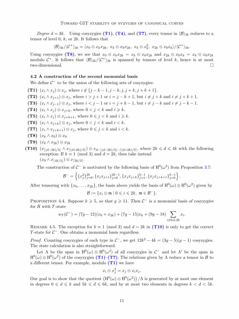
We define C− to be the union of the following sets of cosyzygies:

(T1) (xi ∧ xj)⊗ xj , where i 6∈ j − k − 1, j − k, j, j + k, j + k + 1.(T2) (xi ∧ xj+1)⊗ xj , where i > j + 1 or i = j − k + 1, but i 6= j + k and i 6= j + k + 1.

(T3) (xi ∧ xj−1)⊗ xj , where i < j − 1 or i = j + k − 1, but i 6= j − k and i 6= j − k − 1.

(T4) (xi ∧ xj)⊗ xj+k, where 0 < j < k and i > k.

(T5) (xi ∧ xj)⊗ xj+k+1, where 0 6 j < k and i > k.

(T6) (xi ∧ xj+k)⊗ xj , where 0 < j < k and i < k.

(T7) (xi ∧ xj+k+1)⊗ xj , where 0 6 j < k and i < k.

(T8) (xk ∧ x0)⊗ x0(T9) (xk ∧ x2k)⊗ x2k

(T10) (xb(d−2k)/3c ∧ xd(d+2k)/3e) ⊗ xd−b(d−2k)/3c−d(d+2k)/3e, where 2k 6 d 6 4k with the followingexception: If k ≡ 1 (mod 3) and d = 2k, then take instead(x0 ∧ xb4k/3c)⊗ xd2k/3e.

The construction of C− is motivated by the following basis of H0(ω2) from Proposition 3.7:

B− =x2j2kj=0, xjxj+12k−1j=0 , xjxj+k

k−1j=1 , xjxj+k+1k−1j=0

.

After tensoring with x0, . . . , x2k, the basis above yields the basis of H0(ω)⊗H0(ω2) given by

B := xi ⊗m | 0 6 i 6 2k, m ∈ B−.

Proposition 4.4. Suppose k > 5, so that g > 11. Then C− is a monomial basis of cosyzygiesfor R with T -state

wT (C−) = (7g − 12)(x0 + x2k) + (7g − 15)xk + (9g − 18)∑

i 6=0,k,2k

xi.

Remark 4.5. The exception for k ≡ 1 (mod 3) and d = 2k in (T10) is only to get the correctT -state for C−. One obtains a monomial basis regardless.

Proof. Counting cosyzygies of each type in C−, we get 12k2 − 4k = (3g − 5)(g − 1) cosyzygies.The state calculation is also straightforward.

Let Λ be the span in H0(ω) ⊗ H0(ω2) of all cosyzygies in C− and let Λ′ be the span inH0(ω)⊗H0(ω2) of the cosyzygies (T1)–(T7). The relations given by Λ reduce a tensor in B toa different tensor. For example, modulo (T1) we have

xi ⊗ x2j = xj ⊗ xixj .

Our goal is to show that the quotient(H0(ω)⊗H0(ω2)

)/Λ is generated by at most one element

in degrees 0 6 d 6 k and 5k 6 d 6 6k, and by at most two elements in degrees k < d < 5k.

11


Proposition 4.6 does most of the heavy lifting towards this goal and, for the sake of the argument,we assume its statement for now.

By Proposition 4.6 and Remark 4.7,(H0(ω)⊗H0(ω2)

)/Λ′ is generated by one element in

degrees 0 6 d < k and 5k < d 6 6k, by two elements in degrees k 6 d < 2k and 4k < d 6 5kand by three elements in degrees 2k 6 d 6 4k. Therefore to complete the argument, it suffices toprove that the cosyzygies (T8) and (T9) impose nontrivial linear relations on the two generatorsin degree k and 5k, respectively, and that the cosyzygy (T10) imposes a nontrivial linear relationon the three generators in degrees 2k 6 d 6 4k.

Let d = k. The two generators of(H0(ω)⊗H0(ω2)

)/Λ′ in this degree are

σ1 := xk/3 ⊗ xbk/3cxdk/3e, and

σ2 := xk ⊗ x20.

The relation imposed by (T8) is

xk ⊗ x20 = x0 ⊗ x0xk.It is easy to see that modulo (T1), (T2), and (T3), we have

x0 ⊗ x0xk = x0 ⊗ xbk/2cxdk/2e = σ1.

Therefore, (T8) imposes the nontrivial relation

σ2 = σ1.

The case of d = 5k follows symmetrically.

Let 2k 6 d 6 4k. The three generators of(H0(ω)⊗H0(ω2)

)/Λ′ in degree d are

σ1 := xd/3 ⊗ xdd/3exbd/3c,σ2 := xd(d+2k)/3e ⊗ xb(d−k)/3cx(d−k)/3, and

σ3 := xb(d−2k)/3c ⊗ x(d+k)/3xd(d+k)/3e.

For brevity, set ` = d(d+ 2k)/3e and s = b(d− 2k)/3c. The relation imposed by (T10) is

x` ⊗ xsxd−`−s = xs ⊗ x`xd−`−s. (13)

Assume that d 6 3k; the case of d > 3k follows symmetrically. Since d 6 3k, we have

s < b(d− k)/3c 6 (d− k)/3 < d− `− s 6 k.

On the left hand side of (13), we have by Lemma 3.8

x` ⊗ xsxd−`−s = x` ⊗ xb(d−k)/3cx(d−k)/3= σ2.

On the right hand side of (13), working modulo (T6)–(T7), and applying Lemma 3.8, we get

xs ⊗ x`xd−`−s = λxs ⊗ x(d+k)/3xd(d+k)/3e + µxs ⊗ xb(d−s−k)/2cxd(d−s+k)/2e= λσ3 + µxd(d−s+k)/2e ⊗m, where m is balanced,

= λσ3 + µ(ασ1 + βσ2 + γσ3),

where the last step uses Proposition 4.6. Furthermore, since k > 5, we have d(d − s + k)/2e >d(d + 2k)/3e. Hence Proposition 4.6 (Part 2(c)) implies that α < 0. Thus, (T10) imposes therelation

σ2 = λσ3 + µ(ασ1 + βσ2 + γσ3).

12


If µ = 0, then this relation is clearly nontrivial. If µ 6= 0, the non-vanishing of the coefficient ofσ1 shows that the relation is nontrivial.

Finally, we verify that the exceptional cosyzygy in (T10) for k ≡ 1 (mod 3) and d = 2kimposes a nontrivial relation. The argument is almost the same. In this case, the cosyzygy gives

xb4k/3c ⊗ x0xd2k/3e = x0 ⊗ xd2k/3exb4k/3c. (14)

Reducing the left hand side of (14) modulo (T1)–(T7), we get

xb4k/3c ⊗ x0xd2k/3e = xb4k/3c ⊗m, where m is balanced,

= ασ1 + βσ2 + γσ3.

Since b(d− 2k)/3c 6 b4k/3c 6 d(d+ 2k)/3e, Proposition 4.6 (Part 2(b)) implies that α > 0.

Reducing the right hand side of (14), we get

x0 ⊗ xd2k/3exb4k/3c = λx0 ⊗ x2k + µx0 ⊗ xbk/2cxd3k/2e, where λ, µ > 0

= λσ3 + µxd3k/2e ⊗m, where m is balanced,

= λσ3 + µ(α′σ1 + β′σ2 + γ′σ3).

Since d3k/2e > d(d + 2k)/3e, Proposition 4.6 (Part 2(c)) implies that α′ < 0. Thus, (T10)imposes

ασ1 + βσ2 + γσ3 = λσ3 + µ(α′σ1 + β′σ2 + γ′σ3).

Since α > 0 whereas µα′ < 0, the relation is nontrivial.

Before moving onto the key technical results needed in the proof of Proposition 4.4, weintroduce some additional terminology. We call the forms x2j and xjxj+1 balanced and the formsxjxj+k and xjxj+k+1 k-balanced. Likewise, we call a tensor xi⊗m balanced (resp. k-balanced) if mis balanced (resp. k-balanced). Finally, we call a balanced tensor xi⊗m of degree d well-balancedif b(d− 2k)/3c 6 i 6 d(d+ 2k)/3e. Equivalently, a balanced tensor xi ⊗ xsx` is well-balanced ifmax(|i− s|, |i− `|) 6 k + 1.

Proposition 4.6. (Part 1) Every element of(H0(ω)⊗H0(ω2)

)/Λ′ can be uniquely expressed

as a linear combination of the following tensors:

Type 1

xi ⊗ x2i , where 0 6 i 6 2kxi ⊗ xixi+1, where 0 6 i 6 2k − 1xi ⊗ xi−1xi, where 1 6 i 6 2k

Type 2

xi+k ⊗ x2i , where 0 6 i 6 kxi+k+1 ⊗ x2i , where 0 6 i 6 k − 1xi+k+1 ⊗ xixi+1, where 0 6 i 6 k − 1

Type 3

xi−k ⊗ x2i , where k 6 i 6 2kxi−k−1 ⊗ x2i , where k + 1 6 i 6 2kxi−k−1 ⊗ xixi−1, where k + 1 6 i 6 2k

(Part 2) Furthermore, let 2k 6 d 6 4k. Then there is precisely one tensor of degree d of eachType 1–3. Suppose the balanced tensor τ = xi ⊗ xb(d−i)/2cxd(d−i)/2e is expressed as

τ = ασ1 + βσ2 + γσ3,

where σt is of Type t. Then,

(a) α+ β + γ = 1;

13


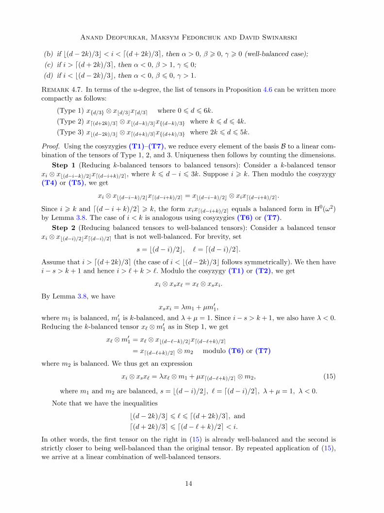
(b) if b(d− 2k)/3c < i < d(d+ 2k)/3e, then α > 0, β > 0, γ > 0 (well-balanced case);

(c) if i > d(d+ 2k)/3e, then α < 0, β > 1, γ 6 0;

(d) if i < b(d− 2k)/3c, then α < 0, β 6 0, γ > 1.

Remark 4.7. In terms of the u-degree, the list of tensors in Proposition 4.6 can be written morecompactly as follows:

(Type 1) xd/3 ⊗ xbd/3cxdd/3e where 0 6 d 6 6k.

(Type 2) xd(d+2k)/3e ⊗ xb(d−k)/3cx(d−k)/3 where k 6 d 6 4k.

(Type 3) xb(d−2k)/3c ⊗ xd(d+k)/3ex(d+k)/3 where 2k 6 d 6 5k.

Proof. Using the cosyzygies (T1)–(T7), we reduce every element of the basis B to a linear com-bination of the tensors of Type 1, 2, and 3. Uniqueness then follows by counting the dimensions.

Step 1 (Reducing k-balanced tensors to balanced tensors): Consider a k-balanced tensorxi ⊗ xb(d−i−k)/2cxd(d−i+k)/2e, where k 6 d − i 6 3k. Suppose i > k. Then modulo the cosyzygy(T4) or (T5), we get

xi ⊗ xb(d−i−k)/2cxd(d−i+k)/2e = xb(d−i−k)/2c ⊗ xixd(d−i+k)/2e.

Since i > k and d(d − i + k)/2e > k, the form xixd(d−i+k)/2e equals a balanced form in H0(ω2)by Lemma 3.8. The case of i < k is analogous using cosyzygies (T6) or (T7).

Step 2 (Reducing balanced tensors to well-balanced tensors): Consider a balanced tensorxi ⊗ xb(d−i)/2cxd(d−i)/2e that is not well-balanced. For brevity, set

s = b(d− i)/2c, ` = d(d− i)/2e.

Assume that i > d(d+ 2k)/3e (the case of i < b(d−2k)/3c follows symmetrically). We then havei− s > k + 1 and hence i > `+ k > `. Modulo the cosyzygy (T1) or (T2), we get

xi ⊗ xsx` = x` ⊗ xsxi.

By Lemma 3.8, we have

xsxi = λm1 + µm′1,

where m1 is balanced, m′1 is k-balanced, and λ+ µ = 1. Since i− s > k+ 1, we also have λ < 0.Reducing the k-balanced tensor x` ⊗m′1 as in Step 1, we get

x` ⊗m′1 = x` ⊗ xb(d−`−k)/2cxd(d−`+k)/2e= xd(d−`+k)/2e ⊗m2 modulo (T6) or (T7)

where m2 is balanced. We thus get an expression

xi ⊗ xsx` = λx` ⊗m1 + µxd(d−`+k)/2e ⊗m2, (15)

where m1 and m2 are balanced, s = b(d− i)/2c, ` = d(d− i)/2e, λ+ µ = 1, λ < 0.

Note that we have the inequalities

b(d− 2k)/3c 6 ` 6 d(d+ 2k)/3e, and

d(d+ 2k)/3e 6 d(d− `+ k)/2e < i.

In other words, the first tensor on the right in (15) is already well-balanced and the second isstrictly closer to being well-balanced than the original tensor. By repeated application of (15),we arrive at a linear combination of well-balanced tensors.

14


Step 3 (Reducing the well-balanced tensors): We now show that all well-balanced tensorsreduce to linear combinations of tensors of Type 1, 2, and 3. We will make use of the followingresult.

Lemma 4.8. Let τ = xi ⊗ xb(d−i)/2cxd(d−i)/2e be a well-balanced tensor of degree d. Modulo(T1)–(T7), we have a reduction

τ = λτ1 + µτ2, (16)

where τ1 and τ2 are well-balanced, λ + µ = 1, and λ, µ > 0. Moreover, if τ is not of Type 2or 3, then λ > 0. And, if τ is not of Type 1, 2, or 3, then τ1 = xj ⊗ xb(d−j)/2cxd(d−j)/2e, where|d/3 − j| < |d/3 − i|, and τ1 is not of Type 2 or 3.

Proof of the lemma. Let τ = xi ⊗ xb(d−i)/2cxd(d−i)/2e. For brevity, set s = b(d − i)/2c and ` =d(d− i)/2e. If i = ` or i = s, then τ is of Type 1. In this case, we take τ1 = τ and λ = 1, µ = 0.If both xix` and xixs are k-balanced, then τ is of Type 2 or 3. In this case, we take τ2 = τ andλ = 0, µ = 1. Suppose neither of these is the case. We consider the case of i > `; the case of i < sfollows symmetrically. Note that ` satisfies

(d− k)/3 6 ` 6 (d+ k)/3. (17)

We first treat the special case i = s + k. Since not both xix` and xixs are k-balanced, wemust have s = `− 1. Therefore, we get

τ = xi ⊗ x`−1x`= x`−1 ⊗ xix` modulo (T3)

= λx`−1 ⊗m1 + µx`−1 ⊗ x`+kx`−1,where m1 is balanced, λ > 0, µ > 0, and λ+ µ = 1 (Lemma 3.8),

= λx`−1 ⊗m1 + µx`+k ⊗ x`−1x`−1 modulo (T6)

= λτ1 + µτ2, as desired.

Now assume that i 6= s+ k. Then 0 < i− ` 6 i− s < k. In this case, we get

τ = xi ⊗ xsx`= x` ⊗ xsxi modulo (T1) or (T2).

We now write using Lemma 3.8

xsxi = λm1 + µm′1,

where m1 is balanced, m′1 is k-balanced and λ+ µ = 1. Since 0 < i− s < k, we have λ > 0 andµ > 0. Reducing the k-balanced tensor x` ⊗m′1 as in Step 1, we get

x` ⊗m′1 = xp ⊗m2,

where m2 is balanced and

p =

b(d− `− k)/2c if ` > k,

d(d− `+ k)/2e if ` < k.

In either case, (17) implies that

b(d− 2k)/3c 6 p 6 d(d+ 2k)/3e.

Setting τ1 = x` ⊗m1 and τ2 = xp ⊗m2, we thus get

τ = λτ1 + µτ2,

15


τ

τ1 τ2

λ µ

Figure 1. The relations among well-balanced tensors as a Markov chain

as claimed.

Finally, we note that if τ = xi ⊗ xsx` was not of Type 1, 2, or 3, then by construction τ1 haslevel j where either j = s in the case of i = s + k, or j = ` in all other cases. In either case, itis clear that |d/3 − j| < |d/3 − i|. (Informally, this means that τ1 is closer to being Type 1than τ .) This finishes the proof of the lemma.

We continue the proof of Proposition 4.6. Let Ω be the set of well-balanced tensors. Define alinear operator P : C〈Ω〉 → C〈Ω〉 that encodes (16), namely

P : τ 7→ λτ1 + µτ2.

By Lemma 4.8, we can interpret P as a Markov process on Ω (see Figure 1). Notice that theabsorbing states of this Markov chain are precisely the tensors of Type 1, 2, and 3. Furthermore,from every other tensor, the path τ → τ1 → . . . eventually leads to a tensor of Type 1, again byLemma 4.8. As a result, P is an absorbing Markov chain. By basic theory of Markov chains, forevery v ∈ C〈Ω〉, the limit limn→∞ P

nv exists and is supported on the absorbing states. Takingv = 1 · τ , we conclude that τ reduces to a linear combination of the absorbing states. We thusget a linear relation

τ = ασ1 + βσ2 + γσ3,

where σt is of Type t, as claimed.

The above analysis also lets us deduce the claims about the coefficients from Part 2 of theproposition. Let 2k 6 d 6 4k. Say τ = xi ⊗ xsx` reduces as

τ = ασ1 + βσ2 + γσ3,

where σt is of Type t.

For Part 2(a), we note that α + β + γ = 1 follows by passing to H0(ω3) and comparing thecoefficients of ud.

For Part 2(b), assume that b(d − 2k)/3c < i < d(d + 2k)/3e. Then τ is well-balanced. Thenon-negativity of P implies the non-negativity of α, β, and γ. Furthermore, since there is a pathof positive weight from τ to σ1, we have α > 0.

For Part 2(c), note that if i = d(d+2k)/3e, then α = 0, β = 1, and γ = 0. For i > d(d+2k)/3e,we show by descending induction on i that α < 0 and γ 6 0. Then since α+β+γ = 1, it followsthat β > 1. For the induction, recall the reduction (15):

τ = λx` ⊗m1 + µxd(d−`+k)/2e ⊗m2,

where the mi are balanced, λ < 0, µ > 0, and λ+ µ = 1. Recall also the inequalities

b(d− 2k)/3c 6 ` 6 d(d+ 2k)/3e and

d(d+ 2k)/3e 6 d(d− `+ k)/2e < i.

16


Except in the extreme case (d, i) = (2k, 2k), both inequalities in the first line are strict. Say wehave the reductions

x` ⊗m1 = α′σ1 + β′σ2 + γ′σ3, and

xd(d−`+k)/2e ⊗m2 = α′′σ1 + β′′σ2 + γ′′σ3.

By Part 2(b), we have α′ > 0, and γ′ > 0. By the inductive assumption, we have α′′ 6 0, andγ′′ 6 0. Since λ < 0 and µ > 0 in (4.2), we conclude the induction step. In the extreme case(d, i) = (2k, 2k), the reduction (4.2) becomes

τ = λσ3 + µxd3k/2e ⊗m2.

The assertion now follows from that for xd3k/2e ⊗m2.

Finally, Part 2(d) follows symmetrically from Part 2(c).

4.3 A construction of the third (and final!) monomial basis

Let C? be the union of the following sets of cosyzygies:

(S1) The cosyzygies (T1)–(T9) in the description of C−.

(S2) (xd−k ∧ x0)⊗ xk for 2k 6 d < 3k,

(S3) (x2k ∧ x0)⊗ xk(S4) (xd−3k ∧ x2k)⊗ xk for 3k < d 6 4k.

Proposition 4.9. C? is a monomial basis of cosyzygies for R with T -state

wT (C?) =15g − 29

2(x0 + x2k) + (8g − 16)xk + (9g − 20)

∑i 6=0,k,2k

xi

Proof. Let Λ′ be the span in H0(ω) ⊗ H0(ω2) of the cosyzygies in (S1). Then by Proposition4.6, the quotient

(H0(ω)⊗H0(ω2)

)/Λ′ is generated by one element in degrees 0 6 d 6 k and

5k 6 d 6 6k, by two elements in degrees k < d < 2k and 4k < d < 5k, and by three elementsin degrees 2k 6 d 6 4k. It suffices to prove that the cosyzygies (S2)–(S4) impose a nontriviallinear relation among the three generators in degrees 2k 6 d 6 4k.

Let 2k 6 d < 3k. Recall that the three generators in this degree are

σ1 := xd/3 ⊗ xdd/3exbd/3c,σ2 := xd(d+2k)/3e ⊗ xb(d−k)/3cx(d−k)/3, and

σ3 := xb(d−2k)/3c ⊗ x(d+k)/3xd(d+k)/3e.

The relation given by (S2) is

x0 ⊗ xd−kxk = xd−k ⊗ x0xk.

We reduce both sides modulo Λ′. Note that x0⊗xd−kxk = x0⊗m1 and xd−k⊗x0xk = xd−k⊗m2

where the mi are balanced. Modulo Λ′, we have by Proposition 4.6

x0 ⊗m1 = ασ1 + βσ2 + γσ3 , and

xd−k ⊗m2 = α′σ1 + β′σ2 + γ′σ3.

17


The relation imposed by (S2) is therefore

ασ1 + βσ2 + γσ3 = α′σ1 + β′σ2 + γ′σ3. (18)

On one hand, since 0 6 b(d− 2k)/3c, Proposition 4.6 implies that γ > 0, α 6 0, and β 6 0. Onthe other hand, since b(d − 2k)/3c < d − k, we either have α > 0 (if d − k < d(d + 2k)/3e) orβ > 0 (if d(d+ 2k)/3e 6 d− k). In either case, the relation (18) is nontrivial.

The same argument goes through for d = 3k.

The case of 3k < d 6 4k follows symmetrically.

We finish this section with an existence result for monomial bases of cosyzygies in low genus.

Proposition 4.10. As before, R is the balanced ribbon of genus g.

(i) Suppose g = 7. There exists a monomial basis C− of cosyzygies for R with T -state

wT (C−) = 40x0 + 42x1 + 42x2 + 40x3 + 42x4 + 42x5 + 40x6.

(ii) Suppose g = 9. There exists a monomial basis C− of cosyzygies for R with T -state

wT (C−) = 56x0 + 60x1 + 60x2 + 60x3 + 56x4 + 60x5 + 60x6 + 60x7 + 56x8.

Proof. Both statements are proved by explicitly writing down a monomial basis of cosyzygiesof R. We provide details only in the case g = 7, the case of g = 9 being similar. Let C− be thefollowing set of cosyzygies:

(i) u-degree 1: x0 ∧ x1 ⊗ x0.(ii) u-degree 2: x0 ∧ x2 ⊗ x0, x0 ∧ x1 ⊗ x1.(iii) u-degree 3: x0 ∧ x3 ⊗ x0, x0 ∧ x1 ⊗ x2, x0 ∧ x2 ⊗ x1.(iv) u-degree 4: x0 ∧ x4 ⊗ x0, x0 ∧ x3 ⊗ x1, x1 ∧ x2 ⊗ x1, x0 ∧ x2 ⊗ x2.(v) u-degree 5: x0 ∧x5⊗x0, x0 ∧x4⊗x1, x1 ∧x3⊗x1, x1 ∧x2⊗x2, x0 ∧x2⊗x3, x0 ∧x1⊗x4.(vi) u-degree 6: x0 ∧ x6 ⊗ x0, x0 ∧ x5 ⊗ x1, x1 ∧ x4 ⊗ x1, x2 ∧ x3 ⊗ x1, x0 ∧ x2 ⊗ x4, x1 ∧ x2 ⊗

x3, x0 ∧ x3 ⊗ x3, x0 ∧ x1 ⊗ x5.(vii) u-degree 7: x0 ∧ x6 ⊗ x1, x1 ∧ x5 ⊗ x1, x1 ∧ x4 ⊗ x2, x2 ∧ x3 ⊗ x2, x0 ∧ x3 ⊗ x4, x1 ∧ x2 ⊗

x4, x1 ∧ x3 ⊗ x3, x0 ∧ x1 ⊗ x6, x0 ∧ x2 ⊗ x5.(viii) u-degree 8: x2 ∧ x6 ⊗ x0, x2 ∧ x5 ⊗ x1, x2 ∧ x4 ⊗ x2, x0 ∧ x4 ⊗ x4, x2 ∧ x3 ⊗ x3, x1 ∧ x3 ⊗

x4, x1 ∧ x2 ⊗ x5, x1 ∧ x4 ⊗ x3, x0 ∧ x3 ⊗ x5, x0 ∧ x2 ⊗ x6.(ix) u-degree 9: x3 ∧ x6 ⊗ x0, x3 ∧ x5 ⊗ x1, x4 ∧ x5 ⊗ x0, x3 ∧ x4 ⊗ x2, x1 ∧ x4 ⊗ x4, x2 ∧ x3 ⊗

x4, x2 ∧ x5 ⊗ x2, x1 ∧ x3 ⊗ x5, x1 ∧ x2 ⊗ x6, x0 ∧ x3 ⊗ x6.(x) In u-degrees 10 − 18, the cosyzygies are obtained from those above by the Z2-involution

described in Remark 3.2.

A straightforward but tedious linear algebra calculation, which we omit, shows that C− is amonomial basis of cosyzygies for the genus 7 balanced ribbon. The T -state of C− is clearly

40x0 + 42x1 + 42x2 + 40x3 + 42x4 + 42x5 + 40x6.

We note in closing that both parts of the proposition can also be verified by a direct searchusing a computer.

18


5. Semi-stability of the 1st syzygy point

In this section, we prove that the balanced canonical ribbon R has semi-stable 1st syzygy point,thus obtaining our main result. We begin with two preliminary lemmas.

Lemma 5.1. For the balanced canonical ribbon R of odd genus g > 5, we have K1,2(R) = 0.

Proof. The claim follows from the existence of a single monomial basis of cosyzygies. We exhibitedsuch a basis in Proposition 4.3.

Remark 5.2. In the terminology of Bayer and Eisenbud [BE95, p.730], the Clifford index of thegenus 2k + 1 balanced ribbon R is k. Therefore, Proposition 5.1 is an immediately consequenceof Green’s conjecture for R, which is still open to the best of our knowledge.

Recall from Section 4 that we have constructed three monomial bases of cosyzygies for R,namely, C+, C−, and C?, with the following T -states:

wT (C+) = (g2 − 1)(x0 + xk + x2k) + (6g − 6)∑

i 6=0,k,2k

xi ,

wT (C−) = 40x0 + 42x1 + 42x2 + 40x3 + 42x4 + 42x5 + 40x6, if g = 7,

wT (C−) = 56x0 + 60x1 + 60x2 + 60x3 + 56x4 + 60x5 + 60x6 + 60x7 + 56x8, if g = 9,

wT (C−) = (7g − 12)(x0 + x2k) + (7g − 15)xk + (9g − 18)∑

i 6=0,k,2k

xi, if g > 11,

wT (C?) =15g − 29

2(x0 + x2k) + (8g − 16)xk + (9g − 20)

∑i 6=0,k,2k

xi .

Lemma 5.3. Suppose g > 5. Let C+, C−, and C? be the monomial bases of cosyzygies for R,constructed in Section 4. Then the convex hull of the T -states wT (C+), wT (C−), and wT (C?)contains the barycenter

3(3g − 5)(g − 1)

g(2k∑i=0

xi).

Proof. Equivalently, we may show that the 0-state is an effective linear combination of wT (C+),wT (C−), and wT (C?) modulo

∑2ki=0 xi. First we deal with the low genus cases. We note that

wT (C+) = 24(2k∑i=0

xi) if g = 5,

wT (C+) + 6wT (C−) = 288(2k∑i=0

xi) if g = 7,

wT (C+) + 8wT (C−) = 528(

2k∑i=0

xi) if g = 9.

19


Assuming g > 11, we have

wT (C+) = (g − 5)(g − 1)(x0 + xk + x2k) (mod

2k∑i=0

xi) ,

wT (C−) = −(2g − 6)(x0 + x2k)− (2g − 3)xk (mod2k∑i=0

xi) ,

wT (C?) = −3g − 11

2(x0 + x2k)− (g − 4)xk (mod

2k∑i=0

xi) .

Form a positive linear combination L of the last two lines as follows:

L := 6wT (C?) + (g − 3)wT (C−)

= −(2g2 − 3g − 15)(x0 + xk + x2k) (mod

2k∑i=0

xi).

Plainly, the 0-state is a positive linear combination of wT (C+) and L.

Having established that CoSyz1(R) is well-defined in Lemma 5.1, we are now ready to proveour main theorem.

Theorem 5.4. Let g > 5 be odd. The balanced canonical ribbon R of genus g has SLg semi-stable1st syzygy point.

Proof. Because H0(R,ωR) is a multiplicity-free representation of Gm ⊂ Aut(R) by Proposition3.1, it suffices to verify semi-stability of CoSyz1(R) with respect to the maximal torus T actingdiagonally on the distinguished basis x0, . . . , x2k of H0(R,ωR) described in Proposition 3.1.For a proof of this reduction see [MS11, Proposition 4.7], [AFS13, Proposition 2.4], or [Lun75,Cor. 2 and Rem. 1].

The non-zero Plucker coordinates of CoSyz1(R) diagonalizing the action of T are preciselythe monomial bases of cosyzygies for R. The T -semi-stability of CoSyz1(R) now follows fromLemma 5.3 and the Hilbert-Mumford numerical criterion.

Corollary 5.5 (Theorem 2.6). A general canonical curve of odd genus g > 5 has a semi-stable1st syzygy point.

Proof. This follows from the fact that R deforms to a smooth canonical curve [Fon93].

6. Computer calculations

For any given genus, the semi-stability of any syzygy point of the balanced ribbon can in principlebe verified numerically by enumerating all the states and checking that their convex hull containsthe trivial state. We did calculations in Macaulay2 and polymake [GS, GJ] that established GITsemi-stability of the 1st syzygy point of the balanced ribbon for g = 7, 9, 11, 13 and the 2nd

syzygy point for g = 9, 11. (Computations for higher genera appear to be impracticable.) Themain theorem of this paper (on first syzygies) and these calculations on second syzygies (for smallgenus) provide the first evidence for feasibility of Farkas and Keel’s approach to constructing thecanonical model of Mg.

20


References

ACGH85 E. Arbarello, M. Cornalba, P. A. Griffiths, and J. Harris. Geometry of algebraic curves. Vol.I, volume 267 of Grundlehren der Mathematischen Wissenschaften. Springer-Verlag, NewYork, 1985.

AF11a Marian Aprodu and Gavril Farkas. Green’s conjecture for curves on arbitrary K3 surfaces.Compos. Math., 147(3):839–851, 2011.

AF11b Marian Aprodu and Gavril Farkas. Koszul cohomology and applications to moduli. InGrassmannians, moduli spaces and vector bundles, volume 14 of Clay Math. Proc., pages25–50. Amer. Math. Soc., Providence, RI, 2011.

AFS13 Jarod Alper, Maksym Fedorchuk, and David Smyth. Finite Hilbert stability of (bi)canonicalcurves. Invent. Math., 191(3):671–718, 2013.

AFSvdW13 Jarod Alper, Maksym Fedorchuk, David Ishii Smyth, and Frederick van der Wyck. Logminimal model program for the moduli space of stable curves: The second flip, 2013.

BB11 Edoardo Ballico and Silvia Brannetti. Notes on projective normality of reducible curves.Rend. Circ. Mat. Palermo (2), 60(3):371–384, 2011.

BE95 Dave Bayer and David Eisenbud. Ribbons and their canonical embeddings. Trans. Amer.Math. Soc., 347(3):719–756, 1995.

Ein87 Lawrence Ein. A remark on the syzygies of the generic canonical curves. J. DifferentialGeom., 26(2):361–365, 1987.

FJ12 Maksym Fedorchuk and David Jensen. Stability of 2nd Hilbert points of canonical curves.International Mathematics Research Notices, 2012. DOI:10.1093/imrn/rns204.

Fon93 Lung-Ying Fong. Rational ribbons and deformation of hyperelliptic curves. J. AlgebraicGeom., 2(2):295–307, 1993.

Gie77 D. Gieseker. Global moduli for surfaces of general type. Invent. Math., 43(3):233–282, 1977.

Gie82 D. Gieseker. Lectures on moduli of curves, volume 69 of Tata Institute of FundamentalResearch Lectures on Mathematics and Physics. Published for the Tata Institute of Funda-mental Research, Bombay, 1982.

GJ Ewgenij Gawrilow and Michael Joswig. polymake: a framework for analyzing convex poly-topes. Version 2.12, http://www.math.tu-berlin.de/polymake/.

Gre84 Mark L. Green. Koszul cohomology and the geometry of projective varieties. J. DifferentialGeom., 19(1):125–171, 1984.

GS Dan Grayson and Mike Stillman. macaulay2: a software system for research in algebraicgeometry. Version 1.6, http://www.math.uiuc.edu/Macaulay2/.

Has05 Brendan Hassett. Classical and minimal models of the moduli space of curves of genus two.In Geometric methods in algebra and number theory, volume 235 of Progr. Math., pages169–192. Birkhauser Boston, Boston, MA, 2005.

HH09 Brendan Hassett and Donghoon Hyeon. Log canonical models for the moduli space of curves:the first divisorial contraction. Trans. Amer. Math. Soc., 361(8):4471–4489, 2009.

HH13 Brendan Hassett and Donghoon Hyeon. Log minimal model program for the moduli spaceof stable curves: the first flip. Ann. of Math. (2), 177(3):911–968, 2013.

KM09 Steven Lawrence Kleiman and Renato Vidal Martins. The canonical model of a singularcurve. Geom. Dedicata, 139:139–166, 2009.

Lun75 Domingo Luna. Adherences d’orbite et invariants. Invent. Math., 29(3):231–238, 1975.

MS11 Ian Morrison and David Swinarski. Groebner techniques for low degree hilbert stability.Experimental Mathematics, 20(1):34–56, 2011.

Sch91 David Schubert. A new compactification of the moduli space of curves. Compositio Math.,78(3):297–313, 1991.

21

http://www.math.tu-berlin.de/polymake/

http://www.math.uiuc.edu/Macaulay2/


Voi02 Claire Voisin. Green’s generic syzygy conjecture for curves of even genus lying on a K3surface. J. Eur. Math. Soc. (JEMS), 4(4):363–404, 2002.

Voi05 Claire Voisin. Green’s canonical syzygy conjecture for generic curves of odd genus. Compos.Math., 141(5):1163–1190, 2005.

Anand Deopurkar [email protected] of Mathematics, Columbia University, 2990 Broadway, New York, NY 10027

Maksym Fedorchuk [email protected] of Mathematics, Boston College, 140 Commonwealth Avenue, Chestnut Hill, MA02467

David Swinarski [email protected] of Mathematics, Fordham University, 113 W 60th Street, New York, NY 10023

22

mailto:[email protected]



Documents

Toward GIT stability of syzygies of canonical curves · Toward GIT stability of syzygies of canonical curves Anand Deopurkar, Maksym Fedorchuk and David Swinarski Abstract We introduce