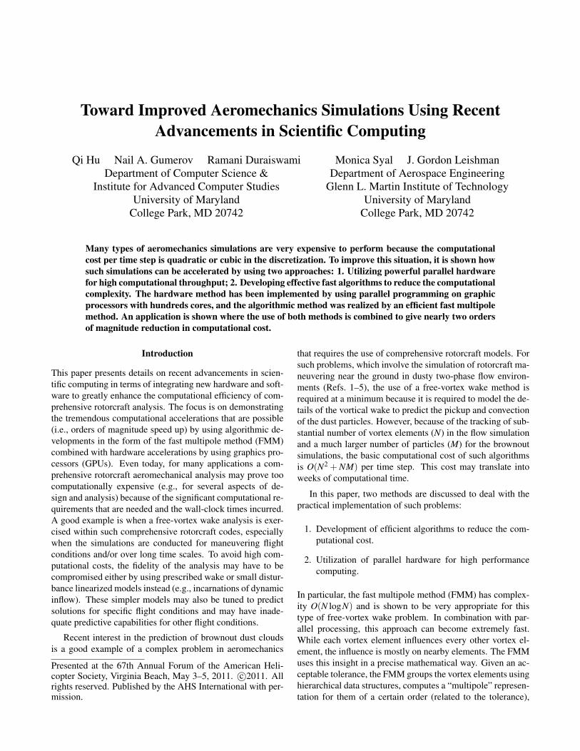
Toward Improved Aeromechanics Simulations Using RecentAdvancements in Scientific Computing

Qi Hu Nail A. Gumerov Ramani DuraiswamiDepartment of Computer Science &

Institute for Advanced Computer StudiesUniversity of Maryland

College Park, MD 20742

Monica Syal J. Gordon LeishmanDepartment of Aerospace Engineering

Glenn L. Martin Institute of TechnologyUniversity of Maryland

College Park, MD 20742

Many types of aeromechanics simulations are very expensive to perform because the computationalcost per time step is quadratic or cubic in the discretization. To improve this situation, it is shown howsuch simulations can be accelerated by using two approaches: 1. Utilizing powerful parallel hardwarefor high computational throughput; 2. Developing effective fast algorithms to reduce the computationalcomplexity. The hardware method has been implemented by using parallel programming on graphicprocessors with hundreds cores, and the algorithmic method was realized by an efficient fast multipolemethod. An application is shown where the use of both methods is combined to give nearly two ordersof magnitude reduction in computational cost.

Introduction

This paper presents details on recent advancements in scien-tific computing in terms of integrating new hardware and soft-ware to greatly enhance the computational efficiency of com-prehensive rotorcraft analysis. The focus is on demonstratingthe tremendous computational accelerations that are possible(i.e., orders of magnitude speed up) by using algorithmic de-velopments in the form of the fast multipole method (FMM)combined with hardware accelerations by using graphics pro-cessors (GPUs). Even today, for many applications a com-prehensive rotorcraft aeromechanical analysis may prove toocomputationally expensive (e.g., for several aspects of de-sign and analysis) because of the significant computational re-quirements that are needed and the wall-clock times incurred.A good example is when a free-vortex wake analysis is exer-cised within such comprehensive rotorcraft codes, especiallywhen the simulations are conducted for maneuvering flightconditions and/or over long time scales. To avoid high com-putational costs, the fidelity of the analysis may have to becompromised either by using prescribed wake or small distur-bance linearized models instead (e.g., incarnations of dynamicinflow). These simpler models may also be tuned to predictsolutions for specific flight conditions and may have inade-quate predictive capabilities for other flight conditions.

Recent interest in the prediction of brownout dust cloudsis a good example of a complex problem in aeromechanics

Presented at the 67th Annual Forum of the American Heli-copter Society, Virginia Beach, May 3–5, 2011. c©2011. Allrights reserved. Published by the AHS International with per-mission.

that requires the use of comprehensive rotorcraft models. Forsuch problems, which involve the simulation of rotorcraft ma-neuvering near the ground in dusty two-phase flow environ-ments (Refs. 1–5), the use of a free-vortex wake method isrequired at a minimum because it is required to model the de-tails of the vortical wake to predict the pickup and convectionof the dust particles. However, because of the tracking of sub-stantial number of vortex elements (N) in the flow simulationand a much larger number of particles (M) for the brownoutsimulations, the basic computational cost of such algorithmsis O(N2 +NM) per time step. This cost may translate intoweeks of computational time.

In this paper, two methods are discussed to deal with thepractical implementation of such problems:

1. Development of efficient algorithms to reduce the com-putational cost.

2. Utilization of parallel hardware for high performancecomputing.

In particular, the fast multipole method (FMM) has complex-ity O(N logN) and is shown to be very appropriate for thistype of free-vortex wake problem. In combination with par-allel processing, this approach can become extremely fast.While each vortex element influences every other vortex el-ement, the influence is mostly on nearby elements. The FMMuses this insight in a precise mathematical way. Given an ac-ceptable tolerance, the FMM groups the vortex elements usinghierarchical data structures, computes a “multipole” represen-tation for them of a certain order (related to the tolerance),

and then further groups them to compute the effect on parti-cles/elements that are even further away. Nearby interactionsare computed directly. The use of data structures allows thisgrouping to be done automatically and efficiently. The hard-ware acceleration was implemented using graphics processors(GPUs) that have a low cost highly parallel architecture con-sisting of hundreds of cores. The results show the feasibilityof this approach for a variety of potential applications in rotor-craft aeromechanics, and show that for some problems com-putational accelerations up to two orders of magnitude fastermay be possible.

Brief Summary of Previous Work

The idea of utilizing parallel computing and multi-core com-puter architectures for aerodynamic computations is not new,with initial work to parallelize free-vortex wake simulationsgoing back at least two decades (Ref. 6). In the context of thepresent approach, recent scientific computing developmentsrelated to the N-body problem are more relevant. Nyland andHarris (Ref. 7) developed a GPU implementation of the N-body simulation. However, their method was based only onhardware accelerations; they simply summed directly all pair-wise interactions and so the cost of the algorithm remainedO(NM) and cannot be scaled to larger problems. Gumerovand Duraiswami (Ref. 8) presented the first realization of theFMM on a GPU, which was a scalable hierarchical algorithm.However, in their work only the most expensive run of thealgorithm was implemented on the GPU, while the data struc-tures required for the FMM were computed on the CPU andtransferred to the GPU.

Stock and Gharakhani (Ref. 9) developed the CPU-GPU-hybrid treecode to accelerate the computations. However, ac-cording to their results its overall performance cannot surpassthe FMM/GPU method implementation method presented inRef. (Ref. 8). Based on the treecode work, Stock et al.(Ref. 10) developed a hybrid Eulerian-Lagrangian method ona multi-core CPU-GPU cluster to model rotor wakes, whichcan simulate high Reynolds number wake flows at reason-able cost. Stone et al. (Ref. 11) also presented a com-bined CPU/GPU parallel algorithm for a hybrid Eulerian-Lagrangian CFD code, where multilevel parallelism wasdemonstrated in the coupled OVERFLOW/VPM algorithm byusing MPI, OpenMP, and CUDA.

GPU Architectures

A graphical processing unit (GPU) is a highly parallel, mul-tithreaded, many-core processor with high computationalpower and memory bandwidth. GPUs were developed orig-inally for graphical rendering to efficiently process single in-structions on multiple data (SIMD). Hence, more transistorson a GPU chip are devoted to data processing rather than to

Fig. 1: GPU computation power (Ref. 13).

Fig. 2: GPU memory bandwidth (Ref. 13).data caching and flow control. Over the years, GPU archi-tectures have evolved tremendously (see Figs. 1 and 2) andcurrent GPUs are capable of both single and double preci-sion computations. GPUs employ a threaded parallel com-putational model. High-end GPUs designed for computationsare already incorporated into many top high performance clus-ters to achieve computational speeds in the high Tera-FLOPs(Ref. 12).

Data on the host (CPU) are transferred to the device (GPU)memory back-and-forth during the entire computational pro-cess (Fig. 3). However, these host-device memory communi-cations are expensive to perform compared to the GPU com-putations. Therefore, one GPU programming philosophy isto minimize the data transfer while processing the data on theGPU as much as possible per data transfer. The memory ar-chitecture on the GPU is hierarchical. In the current NVIDIAFermi architecture (Ref. 14) on which the present simulationswere performed using the FMM, there are four different kindsof memories:

1. Global memory: Device DRAM memory with slow ac-cessing speed but large size. This is used to keep data

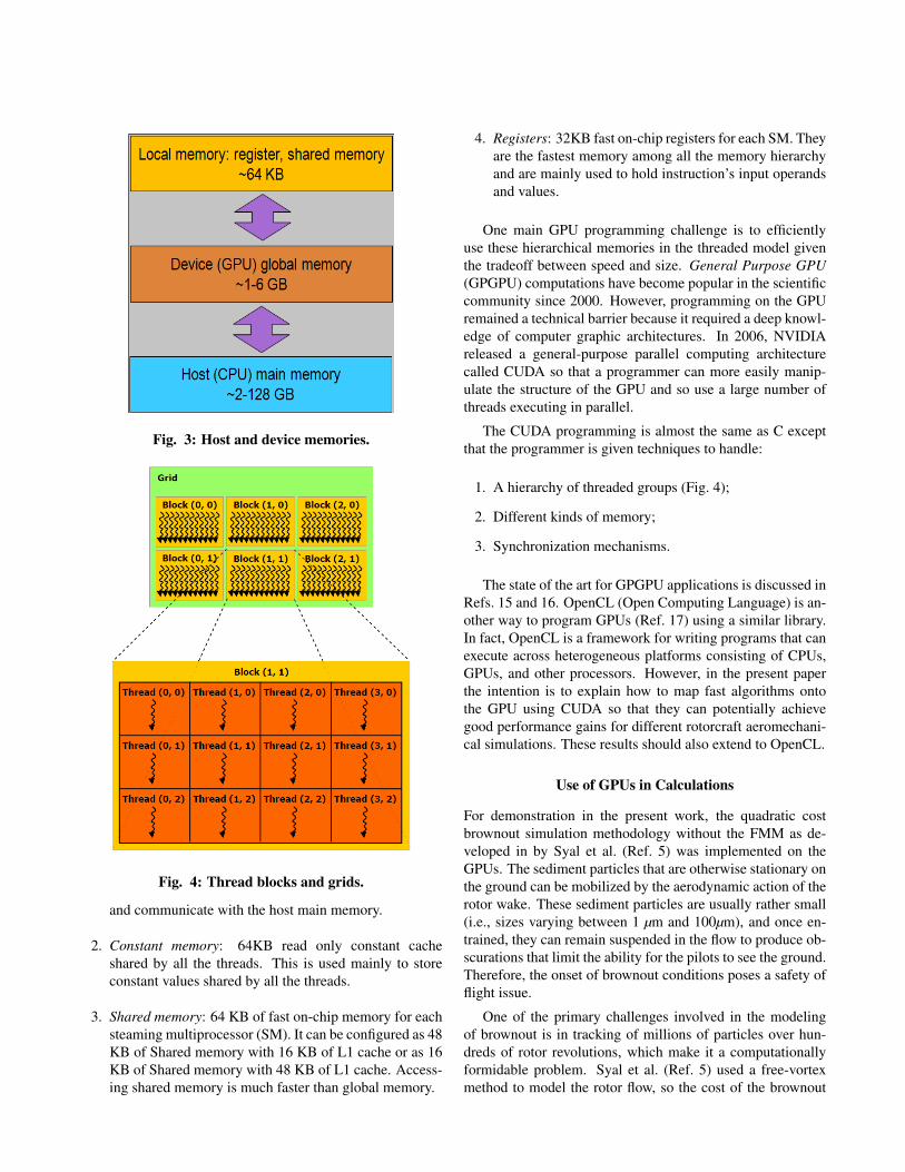
Fig. 3: Host and device memories.

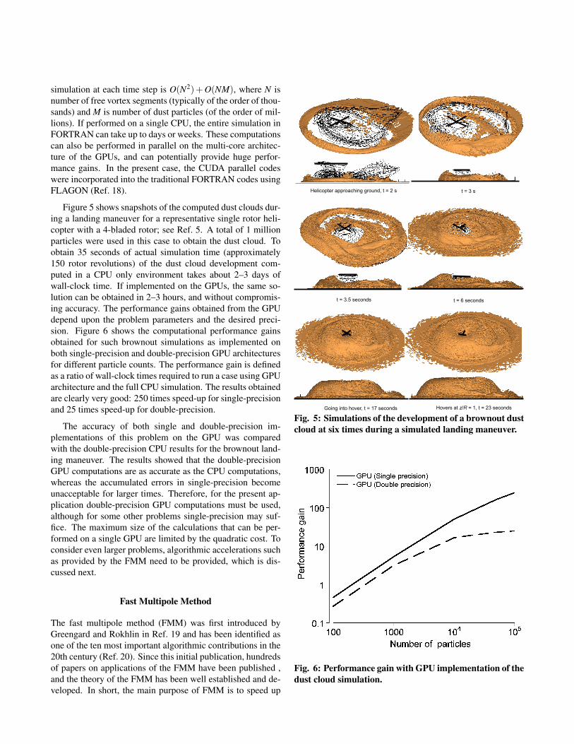
Fig. 4: Thread blocks and grids.

and communicate with the host main memory.

2. Constant memory: 64KB read only constant cacheshared by all the threads. This is used mainly to storeconstant values shared by all the threads.

3. Shared memory: 64 KB of fast on-chip memory for eachsteaming multiprocessor (SM). It can be configured as 48KB of Shared memory with 16 KB of L1 cache or as 16KB of Shared memory with 48 KB of L1 cache. Access-ing shared memory is much faster than global memory.

4. Registers: 32KB fast on-chip registers for each SM. Theyare the fastest memory among all the memory hierarchyand are mainly used to hold instruction’s input operandsand values.

One main GPU programming challenge is to efficientlyuse these hierarchical memories in the threaded model giventhe tradeoff between speed and size. General Purpose GPU(GPGPU) computations have become popular in the scientificcommunity since 2000. However, programming on the GPUremained a technical barrier because it required a deep knowl-edge of computer graphic architectures. In 2006, NVIDIAreleased a general-purpose parallel computing architecturecalled CUDA so that a programmer can more easily manip-ulate the structure of the GPU and so use a large number ofthreads executing in parallel.

The CUDA programming is almost the same as C exceptthat the programmer is given techniques to handle:

1. A hierarchy of threaded groups (Fig. 4);

2. Different kinds of memory;

3. Synchronization mechanisms.

The state of the art for GPGPU applications is discussed inRefs. 15 and 16. OpenCL (Open Computing Language) is an-other way to program GPUs (Ref. 17) using a similar library.In fact, OpenCL is a framework for writing programs that canexecute across heterogeneous platforms consisting of CPUs,GPUs, and other processors. However, in the present paperthe intention is to explain how to map fast algorithms ontothe GPU using CUDA so that they can potentially achievegood performance gains for different rotorcraft aeromechani-cal simulations. These results should also extend to OpenCL.

Use of GPUs in Calculations

For demonstration in the present work, the quadratic costbrownout simulation methodology without the FMM as de-veloped in by Syal et al. (Ref. 5) was implemented on theGPUs. The sediment particles that are otherwise stationary onthe ground can be mobilized by the aerodynamic action of therotor wake. These sediment particles are usually rather small(i.e., sizes varying between 1 µm and 100µm), and once en-trained, they can remain suspended in the flow to produce ob-scurations that limit the ability for the pilots to see the ground.Therefore, the onset of brownout conditions poses a safety offlight issue.

One of the primary challenges involved in the modelingof brownout is in tracking of millions of particles over hun-dreds of rotor revolutions, which make it a computationallyformidable problem. Syal et al. (Ref. 5) used a free-vortexmethod to model the rotor flow, so the cost of the brownout

simulation at each time step is O(N2)+O(NM), where N isnumber of free vortex segments (typically of the order of thou-sands) and M is number of dust particles (of the order of mil-lions). If performed on a single CPU, the entire simulation inFORTRAN can take up to days or weeks. These computationscan also be performed in parallel on the multi-core architec-ture of the GPUs, and can potentially provide huge perfor-mance gains. In the present case, the CUDA parallel codeswere incorporated into the traditional FORTRAN codes usingFLAGON (Ref. 18).

Figure 5 shows snapshots of the computed dust clouds dur-ing a landing maneuver for a representative single rotor heli-copter with a 4-bladed rotor; see Ref. 5. A total of 1 millionparticles were used in this case to obtain the dust cloud. Toobtain 35 seconds of actual simulation time (approximately150 rotor revolutions) of the dust cloud development com-puted in a CPU only environment takes about 2–3 days ofwall-clock time. If implemented on the GPUs, the same so-lution can be obtained in 2–3 hours, and without compromis-ing accuracy. The performance gains obtained from the GPUdepend upon the problem parameters and the desired preci-sion. Figure 6 shows the computational performance gainsobtained for such brownout simulations as implemented onboth single-precision and double-precision GPU architecturesfor different particle counts. The performance gain is definedas a ratio of wall-clock times required to run a case using GPUarchitecture and the full CPU simulation. The results obtainedare clearly very good: 250 times speed-up for single-precisionand 25 times speed-up for double-precision.

The accuracy of both single and double-precision im-plementations of this problem on the GPU was comparedwith the double-precision CPU results for the brownout land-ing maneuver. The results showed that the double-precisionGPU computations are as accurate as the CPU computations,whereas the accumulated errors in single-precision becomeunacceptable for larger times. Therefore, for the present ap-plication double-precision GPU computations must be used,although for some other problems single-precision may suf-fice. The maximum size of the calculations that can be per-formed on a single GPU are limited by the quadratic cost. Toconsider even larger problems, algorithmic accelerations suchas provided by the FMM need to be provided, which is dis-cussed next.

Fast Multipole Method

The fast multipole method (FMM) was first introduced byGreengard and Rokhlin in Ref. 19 and has been identified asone of the ten most important algorithmic contributions in the20th century (Ref. 20). Since this initial publication, hundredsof papers on applications of the FMM have been published ,and the theory of the FMM has been well established and de-veloped. In short, the main purpose of FMM is to speed up

Helicopter approaching ground, t = 2 s

t = 6 seconds t = 3.5 seconds

Hovers at z/R = 1, t = 23 seconds Going into hover, t = 17 seconds

t = 3 s

Fig. 5: Simulations of the development of a brownout dustcloud at six times during a simulated landing maneuver.

Fig. 6: Performance gain with GPU implementation of thedust cloud simulation.

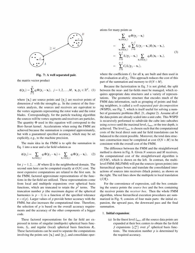
Fig. 7: A well separated pair.

the matrix-vector product

φ(y j) =N

∑i=1

qiΦ(y j−xi), j = 1,2, . . . ,M, xi,y j ∈ Rd , (1)

where xi are source points and y j are receiver points ofdimension d with the strengths qi. In the context of the free-vortex analysis, the sources and receivers are equivalent tothe vortex segments representing the rotor wake and the rotorblades. Correspondingly, for the particle tracking algorithmthe sources will be vortex segments and receivers are particles.The quantity Φ used in this equation will correspond to theBiot–Savart kernel. Accelerations when using the FMM areachieved because the summation is computed approximately,but with a guaranteed specified accuracy, which may be setexplicitly, e.g., to the machine precision.

The main idea in the FMM is to split the summation inEq. 1 into a near and a far field solution as

φ(y j) = ∑xi 6∈Ω(y j)

qiΦ(y j−xi)+ ∑xi∈Ω(y j)

qiΦ(y j−xi), (2)

for j = 1,2, . . . ,M where Ω is the neighborhood domain. Thesecond sum here can be computed exactly at O(N) cost. Themost expensive computations are related to the first sum. Inthe FMM, factored approximate representations of the func-tions in the far-field are utilized. These representations comefrom local and multipole expansions over spherical basisfunctions, which are truncated to retain the p2 terms. Thetruncation number p (the maximum degree of the sphericalharmonics is p− 1) is a function of the specified toleranceε = ε(p). Larger values of p provide better accuracy with theFMM, but also increases the computational time. Therefore,the selection of p is based on the overall accuracy require-ments and the accuracy of the other components of a biggercode.

These factored representations for the far field are ex-pressed in terms of singular (multipole) spherical basis func-tions, Sl , and regular (local) spherical basis functions Rl .These factorizations can be used to separate the computationsinvolving the points sets xi and y j, and consolidate oper-

ations for many points as

∑xi 6∈Ω(y j)

qiΦ(y j−xi)

= ∑xi 6∈Ω(y j)

qi

p−1

∑l=0

Sl(y j−x∗)Rl(xi−x∗),

=p−1

∑l=0

Sl(y j−x∗) ∑xi 6∈Ω(y j)

qiRl(xi−x∗),

=p−1

∑l=0

ClSl(y j−x∗),

(3)

where the coefficients Cl for all xi are built and then used inthe evaluation at all y j. This approach reduces the cost of thispart of the summation and memory to O(N +M).

Because the factorization in Eq. 3 is not global, the splitbetween the near- and far-fields must be managed, which re-quires appropriate data structures and a variety of represen-tations. The geometric structure that encodes much of theFMM data information, such as grouping of points and find-ing neighbors, is called a well-separated pair decomposition(WSPD), see Fig. 7, which is itself useful for solving a num-ber of geometric problems (Ref. 21, chapter 2). Assume all ofthe data points are already scaled into a unit cube. This WSPDis recursively performed to subdivide the cube into subcubesusing octrees until the maximal level, lmax, or the tree depth, isachieved. The level lmax is chosen such that the computationalcosts of the local direct sum and far field translations can bebalanced to the extent possible. Moreover, the total data struc-ture construction must be completed at cost O(N +M) to beconsistent with the overall cost of the FMM.

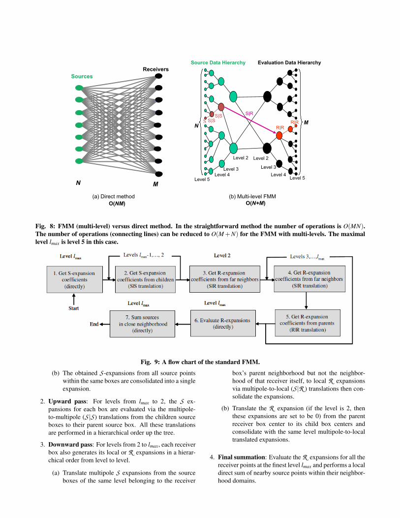
The difference between the FMM and the straightforwardmethod is shown in Fig. 8. Given N sources and M receivers,the computational cost of the straightforward algorithm isO(NM), which is shown on the left. In contrast, the multi-level FMM (MLFMM) will put the sources (green points) intohierarchical space boxes and translate the consolidated inter-actions of sources into receivers (black points), as shown onthe right. The red lines show the multipole to local translation(S |R ).

For the convenience of expression, call the box contain-ing the source points the source box and the box containingthe receiver points the receiver box. Then the whole FMMalgorithm, whose hierarchical execution procedures are sum-marized in Fig. 9, consists of four main parts: the initial ex-pansion, the upward pass, the downward pass and the finalsummation.

1. Initial expansion:

(a) In the finest level lmax, all the source data points areexpanded at their box centers to obtain the far-fieldS expansions C m

n over p2 spherical basis func-tions. The truncation number p is determined bythe required accuracy.

Source Data Hierarchy

N M

Evaluation Data Hierarchy

Level 2

Level 3

Level 4 Level 5

Level 2

Level 3

Level 4 Level 5

S S|S S|S

S|R

R|R R|R

O(NM)

N M

(a) Direct method

Sources

Receivers

(b) Multi-level FMM

O(N+M)

Fig. 8: FMM (multi-level) versus direct method. In the straightforward method the number of operations is O(MN).The number of operations (connecting lines) can be reduced to O(M+N) for the FMM with multi-levels. The maximallevel lmax is level 5 in this case.

Fig. 9: A flow chart of the standard FMM.

(b) The obtained S -expansions from all source pointswithin the same boxes are consolidated into a singleexpansion.

2. Upward pass: For levels from lmax to 2, the S ex-pansions for each box are evaluated via the multipole-to-multipole (S |S ) translations from the children sourceboxes to their parent source box. All these translationsare performed in a hierarchical order up the tree.

3. Downward pass: For levels from 2 to lmax, each receiverbox also generates its local or R expansions in a hierar-chical order from level to level.

(a) Translate multipole S expansions from the sourceboxes of the same level belonging to the receiver

box’s parent neighborhood but not the neighbor-hood of that receiver itself, to local R expansionsvia multipole-to-local (S |R ) translations then con-solidate the expansions.

(b) Translate the R expansion (if the level is 2, thenthese expansions are set to be 0) from the parentreceiver box center to its child box centers andconsolidate with the same level multipole-to-localtranslated expansions.

4. Final summation: Evaluate the R expansions for all thereceiver points at the finest level lmax and performs a localdirect sum of nearby source points within their neighbor-hood domains.

Notice that the evaluations of the nearby source point di-rect sums are independent of the far-field expansions andtranslations, and may be scheduled according to convenience.It is important to balance the costs of these sums and the trans-lations to achieve better computational efficiency and properscaling. Reference 22 gives more details on the algorithm,Ref. 23 describes the translation theory, and Ref. 24 discussesthe different translation methods.

FMM Data Structure

In the previous FMM approach used on GPU implementa-tions (Ref. 8), only the FMM computations were performedon GPUs while the FMM data structures were still developedon CPUs and then transferred to GPUs. This implementationis not the most optimal solution for most of types aerome-chanics problems because of the frequent data transfers be-tween the CPUs and GPUs, which as explained earlier shouldbe minimized for optimal GPU performance. In the presentwork, a novel and efficient technique was developed to fullyimplement the FMM (including data structures) on the GPUs.

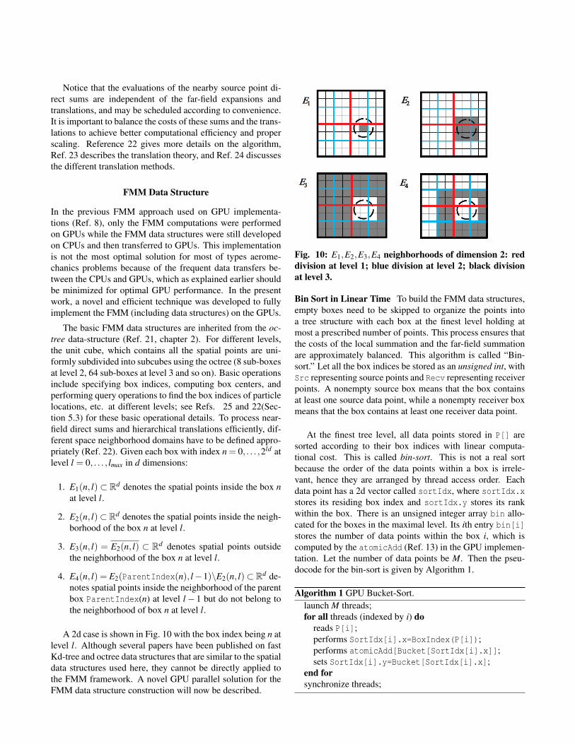
The basic FMM data structures are inherited from the oc-tree data-structure (Ref. 21, chapter 2). For different levels,the unit cube, which contains all the spatial points are uni-formly subdivided into subcubes using the octree (8 sub-boxesat level 2, 64 sub-boxes at level 3 and so on). Basic operationsinclude specifying box indices, computing box centers, andperforming query operations to find the box indices of particlelocations, etc. at different levels; see Refs. 25 and 22(Sec-tion 5.3) for these basic operational details. To process near-field direct sums and hierarchical translations efficiently, dif-ferent space neighborhood domains have to be defined appro-priately (Ref. 22). Given each box with index n = 0, . . . ,2ld atlevel l = 0, . . . , lmax in d dimensions:

1. E1(n, l) ⊂ Rd denotes the spatial points inside the box nat level l.

2. E2(n, l)⊂Rd denotes the spatial points inside the neigh-borhood of the box n at level l.

3. E3(n, l) = E2(n, l) ⊂ Rd denotes spatial points outsidethe neighborhood of the box n at level l.

4. E4(n, l) = E2(ParentIndex(n), l−1)\E2(n, l)⊂Rd de-notes spatial points inside the neighborhood of the parentbox ParentIndex(n) at level l− 1 but do not belong tothe neighborhood of box n at level l.

A 2d case is shown in Fig. 10 with the box index being n atlevel l. Although several papers have been published on fastKd-tree and octree data structures that are similar to the spatialdata structures used here, they cannot be directly applied tothe FMM framework. A novel GPU parallel solution for theFMM data structure construction will now be described.

Fig. 10: E1,E2,E3,E4 neighborhoods of dimension 2: reddivision at level 1; blue division at level 2; black divisionat level 3.

Bin Sort in Linear Time To build the FMM data structures,empty boxes need to be skipped to organize the points intoa tree structure with each box at the finest level holding atmost a prescribed number of points. This process ensures thatthe costs of the local summation and the far-field summationare approximately balanced. This algorithm is called “Bin-sort.” Let all the box indices be stored as an unsigned int, withSrc representing source points and Recv representing receiverpoints. A nonempty source box means that the box containsat least one source data point, while a nonempty receiver boxmeans that the box contains at least one receiver data point.

At the finest tree level, all data points stored in P[] aresorted according to their box indices with linear computa-tional cost. This is called bin-sort. This is not a real sortbecause the order of the data points within a box is irrele-vant, hence they are arranged by thread access order. Eachdata point has a 2d vector called sortIdx, where sortIdx.xstores its residing box index and sortIdx.y stores its rankwithin the box. There is an unsigned integer array bin allo-cated for the boxes in the maximal level. Its ith entry bin[i]stores the number of data points within the box i, which iscomputed by the atomicAdd (Ref. 13) in the GPU implemen-tation. Let the number of data points be M. Then the pseu-docode for the bin-sort is given by Algorithm 1.

Algorithm 1 GPU Bucket-Sort.launch M threads;for all threads (indexed by i) do

reads P[i];performs SortIdx[i].x=BoxIndex(P[i]);performs atomicAdd[Bucket[SortIdx[i].x]];sets SortIdx[i].y=Bucket[SortIdx[i].x];

end forsynchronize threads;

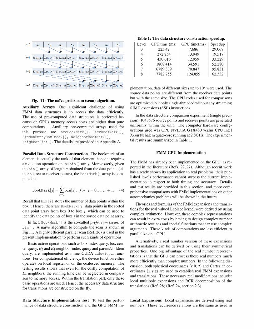
Fig. 11: The naıve prefix sum (scan) algorithm.Auxiliary Arrays One significant challenge of usingFMM data structures is to access the data efficiently.The use of pre-computed data structures is preferred be-cause on GPUs memory access costs are higher than purecomputations. Auxiliary pre-computed arrays used forthis purpose are SrcBookMark[], RecvBookMark[],SrcNonEmptyBoxIndex[], NeighborBookMark[],NeighborList[]. The details are provided in Appendix A.

Parallel Data Structure Construction The bookmark of anelement is actually the rank of that element, hence it requiresa reduction operation on the bin[] array. More exactly, giventhe bin[] array of length n obtained from the data points (ei-ther source or receiver points), the BookMark[] array is com-puted as

BookMark[j] =j

∑i=0

bin[i], f or j = 0, . . . ,n+1, (4)

Recall that bin[i] stores the number of data points within thebox i. Hence, there are BookMark[j] data points in the sorteddata point array from box 0 to box j, which can be used toidentify the data points of box j in the sorted data point array.

In fact, BookMark[] is the so-called prefix sum (scan) ofbin[]. A naıve algorithm to compute the scan is shown inFig 11. A highly efficient parallel scan (Ref. 26) is used in thepresent implementation to perform such kinds of operations.

Basic octree operations, such as box index query, box cen-ter query, E2 and E4 neighbor index query and parent/childrenquery, are implemented as inline CUDA device func-tions. For computational efficiency, the device function eitheroperates on local register or on the coalesced memory. Thetesting results shows that even for the costly computation ofE4 neighbors, the running time can be neglected in compari-son to memory access. Within the translation part, only thesebasic operations are used. Hence, the necessary data structurefor translations are constructed on the fly.

Data Structure Implementation Test To test the perfor-mance of data structure construction and the GPU FMM im-

Table 1: The data structure construction speedup.Level CPU time (ms) GPU time(ms) Speedup

3 223.42 7.686 29.0684 272.254 13.949 19.5175 430.616 12.959 33.2296 1808.414 34.591 52.2807 6789.339 70.847 95.8318 7782.755 124.859 62.332

plementation, data of different sizes up to 107 were used. Thesource data points are different from the receiver data pointsbut with the same size. The CPU codes used for comparisonsare optimized, but only single-threaded without any streamingSIMD extensions (SSE) instructions.

In the data structure comparison experiment (single preci-sion), 1048576 source points and receiver points are generateduniformly within the unit. The computer hardware config-urations used was GPU NVIDIA GTX480 versus CPU IntelXeon Nehalem quad-core running at 2.8GHz. The experimen-tal results are summarized in Table 1.

FMM GPU Implementation

The FMM has already been implemented on the GPU, as re-ported in the literature (Refs. 22, 27). Although recent workhas already shown its application to real problems, their pub-lished levels performance cannot surpass the current imple-mentation in respect to both timing and accuracy. Detailsand test results are provided in this section, and more com-prehensive comparisons with FMM implementations on otheraeromechanics problems will be shown in the future.

Theories and formulas of the FMM expansions and transla-tions for the real valued Laplace kernel were derived by usingcomplex arithmetic. However, these complex representationscan result in extra costs by having to design complex numberarithmetic routines and special functions that can use complexarguments. These kinds of computations are less efficient toparallelize on a GPU.

Alternatively, a real number version of these expansionsand translations can be derived by using their symmetricalproperties. One big advantage of the real number represen-tations is that the GPU can process these real numbers muchmore efficiently than complex numbers. In the following dis-cussion, both spherical coordinates (r,θ,ϕ) and Cartesian co-ordinates (x,y,z) are used to establish real FMM expansionsand translations. These necessary real modifications include:local multipole expansions and RCR decomposition of thetranslations (Ref. 28) (Ref. 24, section 2.3).

Local Expansions Local expansions are derived using realnumbers. These recurrence relations are the same as used in

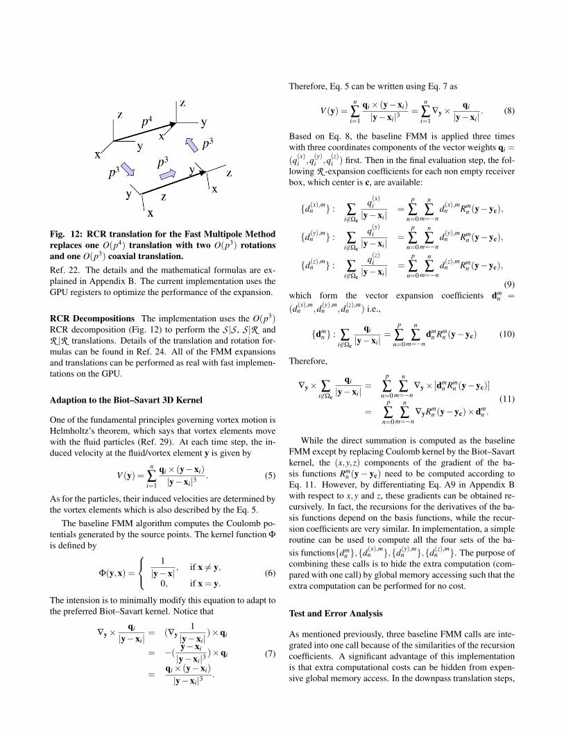
Fig. 12: RCR translation for the Fast Multipole Methodreplaces one O(p4) translation with two O(p3) rotationsand one O(p3) coaxial translation.Ref. 22. The details and the mathematical formulas are ex-plained in Appendix B. The current implementation uses theGPU registers to optimize the performance of the expansion.

RCR Decompositions The implementation uses the O(p3)RCR decomposition (Fig. 12) to perform the S |S , S |R andR |R translations. Details of the translation and rotation for-mulas can be found in Ref. 24. All of the FMM expansionsand translations can be performed as real with fast implemen-tations on the GPU.

Adaption to the Biot–Savart 3D Kernel

One of the fundamental principles governing vortex motion isHelmholtz’s theorem, which says that vortex elements movewith the fluid particles (Ref. 29). At each time step, the in-duced velocity at the fluid/vortex element y is given by

V (y) =n

∑i=1

qi× (y−xi)

|y−xi|3. (5)

As for the particles, their induced velocities are determined bythe vortex elements which is also described by the Eq. 5.

The baseline FMM algorithm computes the Coulomb po-tentials generated by the source points. The kernel function Φ

is defined by

Φ(y,x) =

1

|y−x|, if x 6= y,

0, if x = y.(6)

The intension is to minimally modify this equation to adapt tothe preferred Biot–Savart kernel. Notice that

∇y×qi

|y−xi|= (∇y

1|y−xi|

)×qi

= −( y−xi

|y−xi|3)×qi

=qi× (y−xi)

|y−xi|3.

(7)

Therefore, Eq. 5 can be written using Eq. 7 as

V (y) =n

∑i=1

qi× (y−xi)

|y−xi|3=

n

∑i=1

∇y×qi

|y−xi|. (8)

Based on Eq. 8, the baseline FMM is applied three timeswith three coordinates components of the vector weights qi =

(q(x)i ,q(y)i ,q(z)i ) first. Then in the final evaluation step, the fol-lowing R -expansion coefficients for each non empty receiverbox, which center is c, are available:

d(x),mn : ∑

i6∈Ωc

q(x)i|y−xi|

=p

∑n=0

n

∑m=−n

d(x),mn Rm

n (y−yc),

d(y),mn : ∑

i6∈Ωc

q(y)i|y−xi|

=p

∑n=0

n

∑m=−n

d(y),mn Rm

n (y−yc),

d(z),mn : ∑

i6∈Ωc

q(z)i|y−xi|

=p

∑n=0

n

∑m=−n

d(z),mn Rm

n (y−yc),

(9)which form the vector expansion coefficients dm

n =

(d(x),mn ,d(y),m

n ,d(z),mn ) i.e.,

dmn : ∑

i6∈Ωc

qi

|y−xi|=

p

∑n=0

n

∑m=−n

dmn Rm

n (y−yc) (10)

Therefore,

∇y× ∑i6∈Ωc

qi

|y−xi|=

p

∑n=0

n

∑m=−n

∇y× [dmn Rm

n (y−yc)]

=p

∑n=0

n

∑m=−n

∇yRmn (y−yc)×dm

n .

(11)

While the direct summation is computed as the baselineFMM except by replacing Coulomb kernel by the Biot–Savartkernel, the (x,y,z) components of the gradient of the ba-sis functions Rm

n (y− yc) need to be computed according toEq. 11. However, by differentiating Eq. A9 in Appendix Bwith respect to x,y and z, these gradients can be obtained re-cursively. In fact, the recursions for the derivatives of the ba-sis functions depend on the basis functions, while the recur-sion coefficients are very similar. In implementation, a simpleroutine can be used to compute all the four sets of the ba-sis functionsdm

n ,d(x),mn ,d(y),m

n ,d(z),mn . The purpose of

combining these calls is to hide the extra computation (com-pared with one call) by global memory accessing such that theextra computation can be performed for no cost.

Test and Error Analysis

As mentioned previously, three baseline FMM calls are inte-grated into one call because of the similarities of the recursioncoefficients. A significant advantage of this implementationis that extra computational costs can be hidden from expen-sive global memory access. In the downpass translation steps,

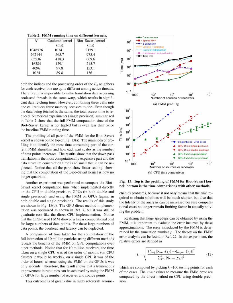
Table 2: FMM running time on different kernels.N Coulomb kernel Biot–Savart kernel

(ms) (ms)1048576 1074.1 2159.1262144 565.7 975.465536 418.3 669.616384 129.1 215.74096 97.8 153.11024 89.8 136.1

both the indices and the processing order of the E4 neighborsfor each receiver box are quite different among active threads.Therefore, it is impossible to make translation data accessingcoalesced threads in the same warp, which results in signifi-cant data fetching time. However, combining three calls intoone call reduces three memory accesses to one. Even thoughthe data being fetched is the same, the total access time is re-duced. Numerical experiments (single precision) summarizedin Table 2 show that the full FMM computation time of theBiot–Savart kernel is not tripled but is even less than twicethe baseline FMM running time.

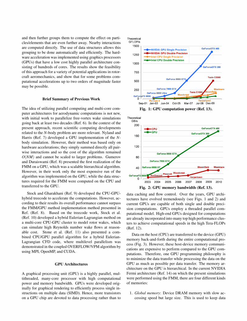
The profiling of all parts of the FMM for the Biot–Savartkernel is shown on the top of Fig. 13(a). The main idea of pro-filing is to identify the most time consuming part of the cur-rent FMM algorithm and how each part scales as the numberof data points increases. The results show that the down passtranslation is the most computationally expensive part and thedata structure construction time is so small that it can be ne-glected. Notice that all the parts show linear scaling, show-ing that the computation of the Biot–Savart kernel is now nolonger quadratic.

Another experiment was performed to compare the Biot–Savart kernel computation time when implemented directlyon the CPU in double precision, GPUs (in both double andsingle precision), and using the FMM on GPUs (again, inboth double and single precision). The results of this studyare shown in Fig. 13(b). The GPU direct method implemen-tation was optimized as shown in Ref. 7, but it was still ofquadratic cost like the direct CPU implementation. Noticethat the GPU-based FMM showed a linear computational costfor large numbers of data points. For these large numbers ofdata points, the overhead and latency can be neglected.

A comparison of time taken for the computation of thefull interaction of 10 million particles using different methodsreveals the benefits of the FMM on GPU computations overother methods. Notice that for 10 million receivers, the timetaken on a single CPU was of the order of months (on CPUclusters it would be weeks), on a single GPU it was of theorder of hours, whereas using the FMM on the GPUs it wasonly seconds. Therefore, this result shows that a tremendousimprovement in run times can be achieved by using the FMMon GPUs for large number of receiver and source points.

This outcome is of great value in many rotorcraft aerome-

(a) FMM profiling

(b) CPU time comparison

Fig. 13: Top is the profiling of FMM for Biot–Savart ker-nel; bottom is the time comparisons with other methods.

chanics problems, because it not only means that the time re-quired to obtain solutions will be much shorter, but also thatthe fidelity of the analysis can be increased because computa-tional costs no longer remain limiting factor in actually solv-ing the problem.

Realizing that huge speedups can be obtained by using theFMM, it is important to evaluate the error incurred by theseapproximations. The error introduced by the FMM is deter-mined by the truncation number p. The theory on the FMMerror analysis can be found in Ref. 22. In this experiment, therelative errors are defined as

ε =

√√√√∑kj=1 |φexact(y j)−φapprox(y j)|2

∑kj=1 |φexact(y j)|2

(12)

which are computed by picking k =100 testing points for eachof the cases. The exact values to measure the FMM error arecomputed by the direct method on CPU using double preci-sion.

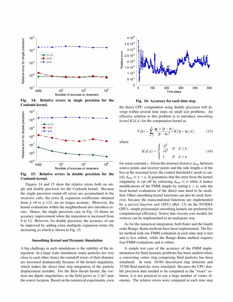
Fig. 14: Relative errors in single precision for theCoulomb kernel.

Fig. 15: Relative errors in double precision for theCoulomb kernel.

Figures 14 and 15 show the relative errors both on sin-gle and double precision for the Coulomb kernel. Becausethe single precision round-off errors are accumulated in therecursive calls, the extra R expansion coefficients obtainedfrom p =8 to p =12, are no longer accurate. Moreover, thekernel evaluations within the neighborhood also introduce er-rors. Hence, the single precision case in Fig. 14 shows noaccuracy improvement when the truncation is increased from8 to 12. However, for double precision, the accuracy of canbe improved by adding extra multipole expansion terms (byincreasing p) which is shown in Fig. 15.

Smoothing Kernel and Dynamic Simulation

A big challenge in such simulations is the stability of the in-tegration. In a large scale simulation, many particles are veryclose to each other, hence the roundoff errors of their distanceare increased dramatically because of the kernel singularity,which makes the direct time step integration of the particledisplacement unstable. For the Biot–Savart kernel, the vor-tices are dipole singularities, so the field grows as 1/|r|2 nearthe source location. Based on the numerical experiments, even

Fig. 16: Accuracy for each time step.the direct CPU computation using double precision will di-verge within several time steps on small size problems. Aneffective solution to this problem is to introduce smoothingkernel K(d,ε) for the computation kernel as

V (y) =n

∑i=1

qi× (y−xi)

|y−xi|3K(|y−xi|,ε), (13)

where

K(d,ε) =

d2

cε2 if d ≤ ε,

1 if d > ε.

(14)

for some constant c. Given the minimal distance dmin betweensource points and receiver points and the side length u of thebox at the maximal level, the control threshold ε needs to sat-isfy dmin ε < u. It guarantees that the error from the kernelsingularity is cut off by enforcing dmin ε while it makesmodifications of the FMM simple by setting ε < u; only thelocal kernel evaluations of the direct sum need to be modi-fied. Other smoothing kernel functions can also be used, how-ever, because the transcendental functions are implementedby a special function unit (SFU) (Ref. 13) on the NVIDIAGPUs, simple polynomial smoothing kernels are preferred forcomputational efficiency. Notice that viscous core models forvortices can be implemented in an analogous way.

As for the numerical integration, both Euler and the fourthorder Runge–Kutta methods have been implemented. The Eu-ler method with one FMM evaluation at each time step is fastand is less robust, while the Runge–Kutta method requiresfour FMM evaluations and is robust.

A simple test case of the accuracy of the FMM imple-mentation for fluid dynamic problems has been studied wherea convecting vortex ring comprising fluid particles has beensimulated. In total, 16384 discretized ring elements and32768 fluid particles were simulated. Because the CPU dou-ble precision data needed to be computed as the “exact” so-lution, it is not practical to use a large number of vortex el-ements. The relative errors were computed at each time step

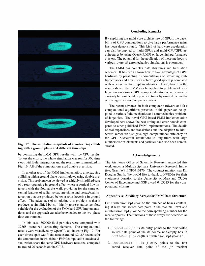
Fig. 17: The simulation snapshots of a vortex ring collid-ing with a ground plane at 4 different time steps.

by comparing the FMM GPU results with the CPU results.To test the errors, the whole simulation was run for 500 timesteps with Euler integration and the results are summarized inFig. 16. All of the computations used double precision.

In another test of the FMM implementation, a vortex ringcolliding with a ground plane was simulated using double pre-cision. This problem can be viewed as a highly simplified caseof a rotor operating in ground effect where a vortical flow in-teracts with the flow at the wall, providing for the same es-sential features of radial vortex stretching and vortex/wall in-teraction that are produced below a rotor hovering in groundeffect. The advantage of simulating this problem is that itproduces a simplified but still highly representative test flowsuitable for the evaluation of the FMM and GPU implementa-tions, and the approach can also be extended to the two-phaseflow environment.

In this case, 500000 fluid particles were computed with32768 discretized vortex ring elements. The computationalresults were visualized by OpenGL, as shown in Fig. 17. Foreach time step, it was found to take around 1.2–2.5 seconds forthe computation in which both FMM computation and data vi-sualization share the same GPU hardware resource, comparedto around 90 seconds on the CPU.

Concluding Remarks

By exploring the multi-core architecture of GPUs, the capa-bility of GPU computations to give large performance gainshas been demonstrated. This kind of hardware accelerationcan also be applied to multi-GPUs and multi-CPU/GPU ar-chitectures by using OpenMP/MPI on large high performanceclusters. The potential for the application of these methods tovarious rotorcraft aeromechanics simulations is enormous.

The FMM has complex data structures and translationschemes. It has been shown how to take advantage of GPUhardware by paralleling its computations on streaming mul-tiprocessors and how it can achieve good speedup comparedwith other sequential implementations. Hence, based on theresults shown, the FMM can be applied to problems of verylarge size on a single GPU equipped desktop, which currentlycan only be completed in practical times by using direct meth-ods using expensive computer clusters.

The recent advances in both computer hardware and fastcomputational algorithms presented in this paper can be ap-plied to various fluid mechanics and aeromechanics problemsof large size. The novel GPU based FMM implementationdeveloped here shows the best timing and error bounds com-pared to other published FMM implementations. The detailsof real expansions and translations and the adaption to Biot–Savart kernel are also gave high computational efficiency onthe GPU. Successful simulations to long times with largenumbers vortex elements and particles have also been demon-strated.

Acknowledgements

The Air Force Office of Scientific Research supported thiswork under a Multidisciplinary University Research Initia-tive, Grant W911NF0410176. The contract monitor was Dr.Douglas Smith. We would like to thank to NVIDIA for theirequipment donation to the University of Maryland CUDACenter of Excellence and NSF award 0403313 for the com-putational clusters.

Appendix A: Auxiliary Arrays for FMM Data Structure

Let numSrcNonEmptyBox be the number of boxes contain-ing at least one source data point in the maximal level andnumRecvNonEmptyBox be the corresponding number for thereceiver points. The functions of these arrays are described asthe following:

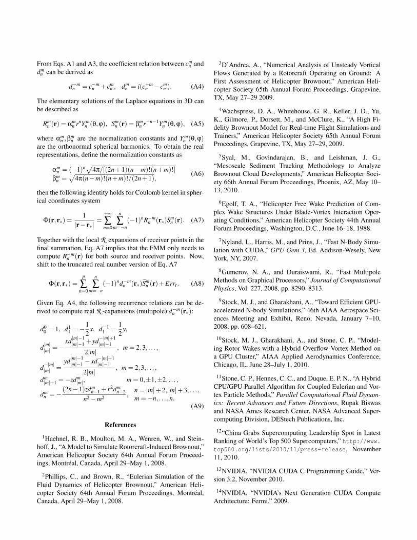
1. SrcBookMark[]: its ith entry points to the first sortedsource data point of the ith source non-empty box inSortedSrc[]. Its length is numSrcNonEmptyBox+1.

2. RecvBookMark[]: its j entry points to the firstsorted receiver data point of the jth receiver

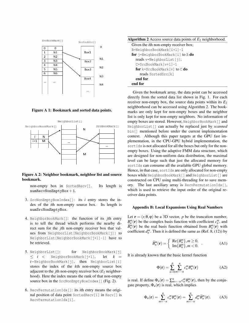
Figure A 1: Bookmark and sorted data points.

Figure A 2: Neighbor bookmark, neighbor list and sourcebookmark.

non-empty box in SortedRecv[]. Its length isnumRecvNonEmptyBox+1.

3. SrcNonEmptyBoxIndex[]: its i entry stores the in-dex of the ith non-empty source box. Its length isnumSrcNonEmptyBox.

4. NeighborBookMark[]: the function of its jth entryis to tell the thread which performs the nearby di-rect sum for the jth non-empty receiver box that val-ues from NeighborList[NeighborBookMark[j]] toNeighborList[NeighborBookMark[j+1]-1] have tobe retrieved.

5. NeighborList[]: for NeighborBookMark[j]≤ i < NeighborBookMark[j+1], let k =i−NeighborBookMark[j], then NeighborList[i]stores the index of the kth non-empty source boxadjacent to the jth non-empty receiver box (E2 neighbor-hood). Here the index means the rank of that non-emptysource box in the SrcNonEmptyBoxIndex[] (Fig. 2).

6. RecvPermutationIdx[]: its ith entry means the origi-nal position of data point SortedRecv[i] in Recv[] isRecvPermutationIdx[i].

Algorithm 2 Access source data points of E2 neighborhood.Given the ith non-empty receiver box;B=NeighborBookMark[i+1]-1for j=NeighborBookMark[i] to B do

reads v=NeighborList[j];C=SrcBookMark[v+1]-1for k=SrcBookMark[v] to C do

reads SortedSrc[k]end for

end for

Given the bookmark array, the data point can be accesseddirectly from the sorted data list shown in Fig. 1. For eachreceiver non-empty box, the source data points within its E2neighborhood can be accessed using Algorithm 2. The book-marks are only kept for non-empty boxes and the neighborlist is only kept for non-empty neighbors. No information ofempty boxes are stored. However, NeighborBookMark[] andNeighborList[] can actually be replaced just by scannedbin[] mentioned before under the current implementationcontext. Although this paper targets at the GPU fast im-plementation, in the CPU-GPU hybrid implementation, thesortIdx is not allocated for all the boxes but only for the non-empty boxes. Using the adaptive FMM data structure, whichare designed for non-uniform data distribution, the maximallevel can be large such that just the allocated memory forsortIdx can consume all the available GPU global memory.Hence, in that case, sortIdx are only allocated for non-emptyboxes while NeighborBookMark[] and NeighborList[] areconstructed on CPU using multi-threading for to save mem-ory. The last auxiliary array is RecvPermutationIdx[],which is used to retrieve the input order of the original re-ceiver data points.

Appendix B: Local Expansions Using Real Numbers

Let r = (r,θ,ϕ) be a 3D vector, p be the truncation number,Bm

n (r) be the complex basis function with coefficient cmn , and

Bmn (r) be the real basis function obtained from Bm

n (r) withcoefficient dm

n . Then it is defined the same as (Ref. 8, (12)) by

Bmn (r) =

ReBm

n ,m≥ 0,ImBm

n ,m < 0. . (A1)

It is already known that the basic kernel function

Φ(r) =p

∑n=0

n

∑m=−n

cmn Bm

n (r) (A2)

is real. If define Φn(r) = ∑nm=−n cm

n Bmn (r), then by the conju-

gate property, Φn(r) is real, which implies

Φn(r) =n

∑m=−n

cmn Bm

n (r) =n

∑m=−n

dmn Bm

n (r). (A3)

From Eqs. A1 and A3, the coefficient relation between cmn and

dmn can be derived as

d−mn = c−m

n + cmn , dm

n = i(c−mn − cm

n ). (A4)

The elementary solutions of the Laplace equations in 3D canbe described as

Rmn (r) = α

mn rnY m

n (θ,ϕ), Smn (r) = β

mn r−n−1Y m

n (θ,ϕ), (A5)

where αmn ,β

mn are the normalization constants and Y m

n (θ,ϕ)are the orthonormal spherical harmonics. To obtain the realrepresentations, define the normalization constants as

αmn = (−1)n

√4π/[(2n+1)(n−m)!(n+m)!]

βmn =

√4π(n−m)!(n+m)!/(2n+1),

(A6)

then the following identity holds for Coulomb kernel in spher-ical coordinates system

Φ(r,r∗) =1

|r− r∗|=

+∞

∑n=0

n

∑m=−n

(−1)nR−mn (r∗)Sm

n (r). (A7)

Together with the local R expansions of receiver points in thefinal summation, Eq. A7 implies that the FMM only needs tocompute R−m

n (r) for both source and receiver points. Now,shift to the truncated real number version of Eq. A7

Φ(r,r∗) =p

∑n=0

n

∑m=−n

(−1)nd−mn (r∗)Sm

n (r)+Errt . (A8)

Given Eq. A4, the following recurrence relations can be de-rived to compute real R -expansions (multipole) d−m

n (r∗):

d00 = 1, d1

1 =−12

x, d−11 =

12

y,

d|m||m| =−xd|m|−1|m|−1 + yd−|m|+1

|m|−1

2|m|, m = 2,3, . . . ,

d−|m||m| =yd|m|−1|m|−1 − xd−|m|+1

|m|−1

2|m|, m = 2,3, . . . ,

dm|m|+1 =−zdm

|m|, m = 0,±1,±2, . . . ,

dmn =−

(2n−1)zdmn−1 + r2dm

n−2

n2−m2 ,n = |m|+2, |m|+3, . . . ,m =−n, . . . ,n.

(A9)

References

1Haehnel, R. B., Moulton, M. A., Wenren, W., and Stein-hoff, J., “A Model to Simulate Rotorcraft-Induced Brownout,”American Helicopter Society 64th Annual Forum Proceed-ings, Montreal, Canada, April 29–May 1, 2008.

2Phillips, C., and Brown, R., “Eulerian Simulation of theFluid Dynamics of Helicopter Brownout,” American Heli-copter Society 64th Annual Forum Proceedings, Montreal,Canada, April 29–May 1, 2008.

3D’Andrea, A., “Numerical Analysis of Unsteady VorticalFlows Generated by a Rotorcraft Operating on Ground: AFirst Assessment of Helicopter Brownout,” American Heli-copter Society 65th Annual Forum Proceedings, Grapevine,TX, May 27–29 2009.

4Wachspress, D. A., Whitehouse, G. R., Keller, J. D., Yu,K., Gilmore, P., Dorsett, M., and McClure, K., “A High Fi-delity Brownout Model for Real-time Flight Simulations andTrainers,” American Helicopter Society 65th Annual ForumProceedings, Grapevine, TX, May 27–29, 2009.

5Syal, M., Govindarajan, B., and Leishman, J. G.,“Mesoscale Sediment Tracking Methodology to AnalyzeBrownout Cloud Developments,” American Helicopter Soci-ety 66th Annual Forum Proceedings, Phoenix, AZ, May 10–13, 2010.

6Egolf, T. A., “Helicopter Free Wake Prediction of Com-plex Wake Structures Under Blade-Vortex Interaction Oper-ating Conditions,” American Helicopter Society 44th AnnualForum Proceedings, Washington, D.C., June 16–18, 1988.

7Nyland, L., Harris, M., and Prins, J., “Fast N-Body Simu-lation with CUDA,” GPU Gem 3, Ed. Addison-Wesely, NewYork, NY, 2007.

8Gumerov, N. A., and Duraiswami, R., “Fast MultipoleMethods on Graphical Processors,” Journal of ComputationalPhysics, Vol. 227, 2008, pp. 8290–8313.

9Stock, M. J., and Gharakhani, A., “Toward Efficient GPU-accelerated N-body Simulations,” 46th AIAA Aerospace Sci-ences Meeting and Exhibit, Reno, Nevada, January 7–10,2008, pp. 608–621.

10Stock, M. J., Gharakhani, A., and Stone, C. P., “Model-ing Rotor Wakes with a Hybrid Overflow-Vortex Method ona GPU Cluster,” AIAA Applied Aerodynamics Conference,Chicago, IL, June 28–July 1, 2010.

11Stone, C. P., Hennes, C. C., and Duque, E. P. N., “A HybridCPU/GPU Parallel Algorithm for Coupled Eulerian and Vor-tex Particle Methods,” Parallel Computational Fluid Dynam-ics: Recent Advances and Future Directions, Rupak Biswasand NASA Ames Research Center, NASA Advanced Super-computing Division, DEStech Publications, Inc.

12“China Grabs Supercomputing Leadership Spot in LatestRanking of World’s Top 500 Supercomputers,” http://www.top500.org/lists/2010/11/press-release, November11, 2010.

13NVIDIA, “NVIDIA CUDA C Programming Guide,” Ver-sion 3.2, November 2010.

14NVIDIA, “NVIDIA’s Next Generation CUDA ComputeArchitecture: Fermi,” 2009.

15Owens, J. D., Luebke, D., Govindaraju, N., Harris, M.,Kr’uger, J., Lefohn, A. E., and Purcell, T., “A Survey ofGeneral- Purpose Computation on Graphics Hardware,” Com-puter Graphics Forum, Vol. 26, (1), March 2007, pp. 80–113.

16Davidson, A., and Owens, J. D., “Toward Techniques forAuto-Tuning GPU Algorithms,” Para 2010: State of the Artin Scientific and Parallel Computing, June 2010.

17NVIDIA, “OpenCL Programming Guide for the CUDAArchitecture,” 3rd edition, 2010.

18Gumerov, N. A., Luo, Y., Duraiswami, R., DeSpain,K., Dorland, B., and Hu, Q., “FLAGON: Fortran-9X Li-brary for GPU Numerics,” GPU Technology Conference,NVIDIA Research Summit, San Jose, CA. Available at http://sourceforge.net/projects/flagon/, October 2009.

19Greengard, L., and Rokhlin, V., “A Fast Algorithm for Par-ticle Simulations,” Journal of Computational Physics, Vol. 73,1987, pp. 325–348.

20Dongarra, J., and Sullivan, F., “The Top 10 Algorithms,”Computing in Science and Engineering, Vol. 2, 2000, pp. 22–23.

21Samet, H., Foundations of Multidimensional and MetricData Structures (The Morgan Kaufmann Series in ComputerGraphics and Geometric Modeling), Morgan Kaufmann Pub-lishers Inc., San Francisco, CA, 2005.

22Gumerov, N. A., and Duraiswami, R., Fast MultipoleMethods for the Helmholtz Equation in Three Dimensions,Elsiever, Oxford, England, 2004.

23Epton, M. A., and Dembart, B., “Multipole TranslationTheory for the Three-Dimensional Laplace and HelmholtzEquations,” SIAM Journal of Scientific Computing, Vol. 16,July 1995, pp. 865–897.

24Gumerov, N. A., and Duraiswami, R., “Comparison of theEfficiency of Translation Operators Used in the Fast Multi-pole Method for the 3D Laplace Equation,” Technical ReportCS-TR-4701, UMIACS-TR-2005-09, University of MarylandDepartment of Computer Science and Institute for AdvancedComputer Studies, April 2005.

25Gumerov, N. A., Duraiswami, R., and Y.A., B., “DataStructures, Optimal Choice of Parameters, and ComplexityResults for Generalized Multilevel Fast Multipole Methods ind-Dimensions,” Technical Report CS-TR-4458; UMIACSTR-2003-28, University of Maryland Department of ComputerScience and Institute for Advanced Computer Studies, April2003.

26Harris, M., Sengupta, S., and Owens, J. D., “Parallel Pre-fix Sum (Scan) with CUDA,” GPU Gems 3, Addison Wesley,New York, NY, August 2007, pp. 851–876.

27Yokota, R., Narumi, T., Sakamaki, R., Kameoka, S., Obi,S., and Yasuoka, K., “Fast Multipole Methods on a Cluster ofGPUs for the Meshless Simulation of Turbulence,” ComputerPhysics Communications, Vol. 180, 2009, pp. 2066–2078.

28White, C. A., and Head-Gordon, M., “Rotating Aroundthe Quartic Angular Momentum Marrier in Fast MultipoleMethod Calculations,” The Journal of Chemical Physics,Vol. 105, September 1996, pp. 5061–5067.

29Batchelor, G. K., An Introduction to Fluid Dynamics, Cam-bridge University Press, New York, NY, February 2000.