Toward Maximum Diversiﬁcation - TOBAM · understanding portfolio construction issues, ... Toward Maximum ... tion works in portfolio construction can be gained fromPublished in:

ITISILLEGALTOREPRODUCE THIS ARTICLEINANY FORMAT

40 TOWARD MAXIMUM DIVERSIFICATION FALL 2008

Diversification has been at thecenter of finance for over 50 years.And to paraphrase Markowitz[1952], diversification is the only

free lunch in finance. Much effort has goneinto developing modern portfolio theorywithin the Markowitz mean-variance frame-work. Perhaps foremost amongst those effortsis the capital asset pricing model (CAPM)developed by Sharpe [1964]. While brilliant inits simplicity and clarity, years of examinationhave led to a vigorous debate about whetherthe assumptions upon which the modeldepends reflect real market conditions andwhether its conclusion can be transposed toactual portfolio management.

A separate set of arguments concerns thedynamic aspects of portfolio construction.Accounting for dynamic changes in the port-folio has led to an examination of thesedynamic changes as a source of return. Fern-holz and Shay [1982] stated that constant-pro-portion portfolios earned additional returnsover the returns earned by buy-and-hold port-folios. Booth and Fama [1992] described theseadditional returns as diversification returns.Although they provide useful insights, the dif-ferent examinations of multiperiod rebalancingeffects are not directly useful for portfolio con-struction because they only deal with port-folio dynamics after the original weights havebeen decided.

Although very useful in describing andunderstanding portfolio construction issues,the mean-variance framework has some prac-tical problems. For example, while variancecan be estimated with a fair level of confi-dence, returns are so much more difficult toestimate that most popular models, such asCAPM and Black-Litterman, have in one wayor another completely put them aside. It isnow increasingly popular to claim that themarket capitalization–weighted indices are notefficient. Several alternative empirical solu-tions have been suggested, such as fundamentalindexation and equal weights.

In this article, we investigate the theo-retical and empirical properties of diversifica-tion as a criterion in portfolio construction. Wecompare the behavior of the resulting port-folio to common, simple strategies, such asmarket cap–weighted indices, minimum-vari-ance portfolios, and equal-weight portfolios.

DEFINITION OF THEDIVERSIFICATION RATIO ANDMOST-DIVERSIFIED PORTFOLIO

We begin by mathematically defining howwe measure the diversification of a portfolio.

Let X1, X2, …, XN be the risky assets ofuniverse U. For simplification, we will considerXi to be stocks. Let V be the covariance matrixof these assets and C the correlation matrix.

Toward MaximumDiversificationYVES CHOUEIFATY AND YVES COIGNARD

YVES CHOUEIFATY

is the head of QuantitativeAsset Management, Europe,at Lehman Brothers inParis, [email protected]

YVES COIGNARD

is the co-deputy head ofQuantitative Asset Manage-ment, Europe, at LehmanBrothers in Paris, [email protected]

Copyright © 2008

Let be the vector of asset volatilities.

Any portfolio P will be noted P = (wp1, wp2, …,wpN), with .

We define the diversification ratio of any portfolio P,denoted D(P), as the following:

(1)

The diversification ratio is the ratio of the weightedaverage of volatilities divided by the portfolio volatility.

Let Γ be a set of linear constraints applied to theweights of portfolio P. One usual set of constraints is thelong-only constraint (i.e., all weights must be positive).The portfolio, which under the set of constraints Γ max-imizes the diversification ratio in universe U, is the Most-Diversified Portfolio, denoted as M(Γ, U).

An intuitive understanding of the way diversifica-tion works in portfolio construction can be gained fromthe following two examples.

Example 1

Suppose we have an investment universe of twostocks, A and B, with a correlation strictly lower than 1,and with respective volatilities of 15% and 30%. In thiscase, diversification means that we want both stocks toequally contribute to portfolio volatility. Their respectiveweights in the Most-Diversified Portfolio would thus be66.6% for stock A and 33.3% for stock B (inversely pro-portional to volatility).

Example 2

Suppose we have an investment universe of threestocks. Let us assume that two are banking stocks with ahigh correlation of 0.9 and that the third stock, a phar-maceutical stock, has a correlation of 0.1 with each of thetwo banking stocks. Suppose, for simplicity, that the volatil-ities are all equal. The weights of the Most-DiversifiedPortfolio, according to the result just obtained, are 25.7%

D PP

P VP( ) = ′ ⋅

′Σ

ΣiN

piw= =1 1

Σ =

⎡

⎣

⎢⎢⎢⎢⎢⎢

⎤

⎦

⎥⎥⎥⎥⎥⎥

σσ

σ

1

2

.

.

N

for each of the banking stocks and 48.6% for the phar-maceutical stock.

THEORETICAL RESULTS

The diversification ratio of any long-only portfoliowill be strictly higher than 1 except when the portfoliois equivalent to a mono-asset portfolio, in which case thediversification ratio will be equal to 1.

If the expected excess returns of assets are propor-tional to their risks (volatilities), then ER(P) = kP′Σ, wherek is a constant, and maximizing D(P) is equivalent to max-imizing , which is the Sharpe ratio of the portfolio.In this case, the Most-Diversified Portfolio is also the tan-gency portfolio.

To provide a better understanding of this ratio, andalso to simplify the math, we transpose the problem to asynthetic universe in which all the stocks have the sameexpected volatility.

Suppose that investors can lend and borrow cash atthe same rate. We can then define the synthetic assets Y1,Y2, …, YN by

where $ is the risk-free asset. We now have the universe,US, of the following assets Y1, Y2, …, YN. In this uni-

verse,

the volatility σSi of Yi is equal to 1, and

In , S is a portfolio composed of the

synthetic assets, and VS is the covariance matrix of the

synthetic assets. If we have S′ΣS = 1, then maximizing

D(S) is equivalent to maximizing under constraints

ΓS. Because all Yi have a normalized volatility of 1 and

because correlation does not change with leverage, VS is

equal to the correlation matrix C of our initial assets, so

1′S V SS

D S S

S V SS

S( ) = ′

′

Σ

ΣS =

⎡

⎣

⎢⎢⎢⎢⎢⎢

⎤

⎦

⎥⎥⎥⎥⎥⎥

1

1

1

.

.

YX

ii

i i

= + −⎛

⎝⎜⎞

⎠⎟σ σ1

1$

ER P

P VP

( )

′

FALL 2008 THE JOURNAL OF PORTFOLIO MANAGEMENT 41

Copyright © 2008

that maximizing the diversification ratio is equivalent to

minimizing

(2)

Thus, in a universe in which all stocks have the samevolatility, we minimize the variance, which is indeed thebenefit we expect from diversification.

When building a real portfolio, we need to recon-struct synthetic assets by holding real assets plus (or minus)some cash. If S = (wS1, wS2, …, wSN) denotes the optimalweights for the synthetic assets, then the optimal port-folio M of real assets will be

PROPERTIES

If C is invertible and Γ = Ø, then S = M(ΓS,US) isunique, and we have the following analytical results:

(3)

The synthetic asset weights, S, are proportional tothe inverse of the correlation matrix C times 1, a vectorof ones the same size as the number of assets.

Once again, we can transform the synthetic assetsback to the portfolio of original assets by dividing eachsynthetic portfolio weight by the volatility of that assetand rescaling the portfolio to be 100% invested. If wedenote the vector of weights of the original assets as M,then we can write

(4)

where σ is a diagonal matrix of the asset volatilities.Now, consider the properties of asset correlation

in the context of the Most-Diversified Portfolio. In asimilar manner, we can calculate the correlation of anarbitrary portfolio P with the Most-Diversified Port-folio M. Because M is inversely proportional to σ andC, we can write

M C∝ − −σ 1 11

S C∝ −11

Mw w w wS S SN

N

Si

ii

N

= −⎛

⎝⎜⎞

⎠⎟=∑1

1

2

2 1

1σ σ σ σ

, , ..., , $⎛⎛

⎝⎜

⎞

⎠⎟

′S CS where κ is a constant factor.Thus,

(5)

This means that the correlation of portfolio P with theMost-Diversified Portfolio M is proportional to the diver-sification ratio of portfolio P, namely D(P).

Now, consider the correlations between single stocksand the Most-Diversified Portfolio. The diversificationratio of a single stock is 1, because there is no diversifi-cation. Using Formula (5), we calculate the correlationof asset i, which has a weight vector wi, whose ith asset’sweight is 1 and other weights are 0, with the vector ofthe Most-Diversified Portfolio holdings M. We obtain

(6)

Remarkably, the correlation of asset i with the Most-Diversified Portfolio is the same for every one of the assets.Thus, we can identify the Most-Diversified Portfolio asbeing the one in which all assets have the same positivecorrelation to it.

The special case that P is the Most-Diversified Port-folio M in Formula (5) leads us to the result that

(7)

so that we have identified the constant κ. Thus, we canrewrite the correlation between a general portfolio P andthe Most-Diversified Portfolio M as the ratio of theirdiversification ratios, as follows:

(8)ρP M

P

D M,

( )

( )=

D

κσ

= M

D M( )

ρ κσi M

M, =

ρ σ σσ σ

σ σκ σσ σ

σ

σκ

P MP M P M

i ii

P

P C M P C C

w

, = ′ = ′

=

− −

∑

1 11

σσκ

σM M

D P= ( )

M C= − −κσ 1 11


Copyright © 2008

with this information we can obtain a single (diversifica-tion) factor model which resembles the CAPM in form,but now identifies the correlation as the ratio of the diver-sification levels,

(9)

where R represents an excess return over cash, and αPand εP are the constant and error terms, respectively, nor-mally associated with regression.

Long-Only Portfolios

In the real world, Γ is usually not empty, and includesthe constraint of having positive weights. As such, theproperties we described for the unconstrained problemare still true for the subuniverse of securities that is com-posed of the stocks selected by the constrained Most-Diversified Portfolio.

The subsequent results focus on the long-only Most-Diversified Portfolio. Two consequences of this are that1) the positivity constraint will reduce the potential impactof estimation errors, and 2) being long-only ensures thatthe portfolio will have a positive exposure to the equityrisk premium.

Thus, all non-zero-weighted assets have the iden-tical correlation to the Most-Diversified Portfolio. Zero-weighted assets, excluded from the Most-DiversifiedPortfolio in the optimization, have correlations to theMost-Diversified Portfolio that are higher than the non-zero-weighted assets in the Most-Diversified Portfolio.This is consistent with identifying the Most-DiversifiedPortfolio subject to the constraints applied.

Other Properties

If all of the stocks in the universe have the samevolatility, then the Most-Diversified Portfolio is equalto the global minimum-variance portfolio. Furthermore, ifwe continuously rebalance the Most-Diversified Port-folio, and because it is a market cap–independentmethodology, the Most-Diversified Portfolio shouldget a significant part of the benefits from diversifica-tion returns when compared to a pure buy-and-holdstrategy (Booth and Fama [1992]).

RD P

D MRP P

P

MM P= + +α

σσ

ε( )

( )

EMPIRICAL RESULTS

In this section, we explain the methodology used inour analysis and the results for Eurozone and U.S. equi-ties. Additionally, we discuss the biases in the method-ology and present an analysis of the performance results.We conclude the section with a review of the issuesrelating to stock selection and the uniqueness of theoptimal portfolio.

Methodology

A number of steps need to be addressed beforetesting the Most-Diversified Portfolio. First, a universeof assets must be selected, and the returns data for theseassets must be collected to cover at least a full marketcycle. Care should be taken to establish that the data areaccurate, particularly in regard to splits, dividends, and,most significantly, survivorship bias.

Given clean returns data, the covariance matrix mustnext be estimated. Because this is the full information setused to construct the portfolio, it is important to examinethe impact of estimation errors on the resulting portfolio.A variety of ways exists to estimate covariances, such assimple windows, decayed weighting, GARCH, andBayesian update methodologies. Although estimationerrors often occur at the levels of volatility and correla-tion, the hierarchies of correlations are more stable. Indeed,we find that portfolios built using differently estimatedcovariance matrices have similar characteristics. Changingthe frequency of data and the estimation period has littleimpact on the final results. Even portfolios built on for-ward-looking covariance matrices (having perfect covari-ance foresight) have only slightly different results thanwhen using historical covariances.

We must also be aware that optimizers tend to allo-cate more risk to factors whose volatility has been under-estimated (see Michaud [1998]). This is especially truefor long–short portfolios built from very large universeswhere multicollinearity is likely. A simple way to addressthis issue is to add positivity constraints to the optimiza-tion program. In the case of multicollinearity, the factthat the optimal portfolio might not be unique is not areal problem for the portfolio manager—it just providesmore choice, as in choosing between equivalent long-only portfolios. It is possible to further limit the impactof estimation errors by adding upper weight limits to theprogram.


Copyright © 2008

For purposes of comparison, we maximize thediversification ratio, defined in Equation (1), at everymonth-end for different universes of securities. We com-pare the results for the long-only Most-Diversified Port-folio with the market cap–weighted benchmark,minimum-variance portfolio, and equal-weight portfolio.We analyze two different regional equity markets, theU.S. and the Eurozone.

We use Standard & Poor’s (S&P) 500 Index data fromDecember 1990 to February 2008 as the daily performanceseries for U.S. equities, and the Dow Jones (DJ) Euro StoxxLarge Cap Index data from December 1990 to February2008 as the daily performance series for Eurozone equities.

The covariance matrix is computed using 250 daysof daily returns. The starting date for the empirical testis December 1991. For computational reasons, we excludefrom the universe, for month-end computations, all stockshaving less than a 250-day price history.

Because the portfolios are long-only, all weightsmust be positive. We also limit the contribution to riskto 4% per asset. In order to conform to an asset managers’framework, we also constrain the month-end weights tocomply with UCITS III rules (i.e., the maximum weightper security is 10%, and the sum of weights above 5%must be lower than 40%).

Results for Eurozone and U.S. Equities

The results of the empirical tests for the Most-Diver-sified Portfolio are summarized in Exhibits 1 and 2. TheMost-Diversified Portfolio consistently delivers superiorrisk-adjusted returns in both regions. As expected, it is con-sistently less risky than the market cap–weighted indices(i.e., volatility is 13.9% versus 17.9% for Eurozone equities,and 12.7% versus 13.4% for U.S. equities). The Most-Diver-sified Portfolio shows a higher Sharpe ratio than the marketcap–weighted benchmark, minimum-variance portfolio,and equal-weight portfolio over the entire period.

In order to further analyze the behavior during dif-ferent market conditions, we split the backtest results intotwo subperiods:

Subperiod 1—1992 to 2000 (i.e., the end of thedot-com bubble)Subperiod 2—2001 to 2008

Biases and Analysis of Performance

It is clear that all market cap–independent method-ologies tend to be less biased toward large capitalizations

than market cap–weighted indices. Therefore, a compar-ison of the Most-Diversified Portfolio to market capital-ization–weighted indices should always show a size bias.Other biases (relative to market capitalization–weightedindices) can appear, even as the inverse of the index’s bias.

To measure the importance of factor bias in theempirical results, we performed a three-factor Fama–French [1993, 1996] regression of the performance of theportfolios versus the market, HML (high-minus-low bookvalue), and SMB (small-minus-big capitalization) factors.The results are shown in Exhibits 3 and 4.

Exhibit 3 shows that for the full period the inter-cept is significantly positive for the most-diversified Euro-zone portfolio, with an annualized excess return (intercept)of 6.0% and a t-stat of 4.14. These figures compare to5.1% and 3.51, respectively, for the minimum-varianceportfolio, and 0.6% and 1.16, respectively, for the equal-weight portfolio. The hierarchy of results is confirmedover the two subperiods.

Exhibit 4 shows results of the same nature for themost-diversified U.S. portfolio, with an annualized excessreturn (intercept) of 3.1% and a t-stat of 1.83. These fig-ures compare to 2.2% and 1.40, respectively, for the min-imum-variance portfolio, and 1.2% and 2.27, respectively,for the equal-weight portfolio.

More broadly, we analyzed the active returns ofthe most-diversified Eurozone portfolio with theLehman Brothers Equity Risk Analysis (ERA) factormodel for the period 1999–2008 (i.e., the period ofavailability for the factor model). The results, shown inExhibit 5, indicate that the dominant factor explainingthe outperformance over the period is specific risk,meaning that about 18% (out of 48%) of the outper-formance cannot be explained by the predefined factorsof the model. This performance arises from real stock-specific risk, omitted common risk factors, and changesin exposure to factors.

Stock Selection Issues and Uniquenessof the Optimal Portfolio

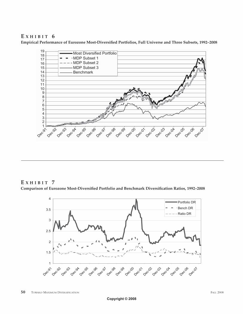
If the correlation matrix is not invertible, the solu-tion may not be unique. But because all possible portfo-lios bring maximum diversification, we are indifferent tothe solution. We see that, in empirical tests, running theMost-Diversified Portfolio model on three subuniverses(obtained by randomly excluding one-third of the uni-verse each time) gives very similar results.


Copyright © 2008

Exhibit 6 shows the performance of the Most-Diversified Eurozone Portfolio and its three subsets versusits benchmark. The same test on the U.S. universe pro-duces similar results. These results show that the Most-Diversified Portfolios tend to allocate risk to risk factorsmuch more than to specific stocks or sectors, even thoughthe average number of stocks in a Most-Diversified Portfoliois relatively low (between 30 and 60).

Diversification Ratio

Exhibit 7 shows the changes in diversification ratiosthrough time for the Most-Diversified Eurozone Port-folio and the Eurozone benchmark. We can see thatalthough the levels of diversification vary through timeas a result of the changes in the levels of correlation, the


E X H I B I T 1Comparison of Eurozone Equity Portfolios, 1992–2008

Note: MDP is the Most-Diversified Portfolio. B represents the market cap–weighted benchmark, the Dow Jones EuroStoxx Large Cap Total Return Index.MV represents a minimum-variance portfolio, and EW represents an equally weighted portfolio, both on the same universe as the benchmark B. The chartshows total return indices.

Copyright © 2008

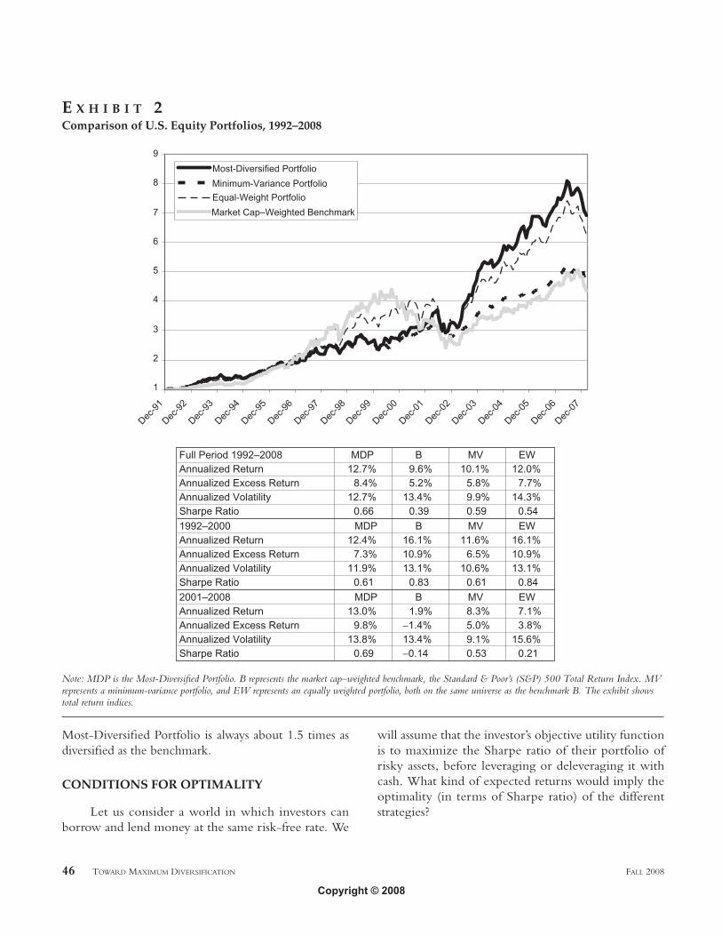
Most-Diversified Portfolio is always about 1.5 times asdiversified as the benchmark.

CONDITIONS FOR OPTIMALITY

Let us consider a world in which investors canborrow and lend money at the same risk-free rate. We

will assume that the investor’s objective utility functionis to maximize the Sharpe ratio of their portfolio ofrisky assets, before leveraging or deleveraging it withcash. What kind of expected returns would imply theoptimality (in terms of Sharpe ratio) of the differentstrategies?


E X H I B I T 2Comparison of U.S. Equity Portfolios, 1992–2008

Note: MDP is the Most-Diversified Portfolio. B represents the market cap–weighted benchmark, the Standard & Poor’s (S&P) 500 Total Return Index. MVrepresents a minimum-variance portfolio, and EW represents an equally weighted portfolio, both on the same universe as the benchmark B. The exhibit showstotal return indices.

Copyright © 2008

Most-Diversified Portfolio

Recall that the Most-Diversified Portfolio is optimalif the stocks’ expected returns are proportional to theirvolatilities; that is, E(Ri) = kσi, where k is a constant factorand σi is the volatility of stock i.

Market Cap–Weighted Benchmark

Considering the CAPM assumptions, a marketcap–weighted benchmark will be optimal, and we canstate

(10)

where E(Ri) is the expected excess return of stock i, E(RB)is the expected excess return of the benchmark (a proxyfor the market portfolio), and ρi,B is the correlationbetween stock i and the benchmark. For simplificationwe assume the risk-free rate is 0%.

If we consider E(RB) and σB to be given for theperiod considered, we have

E(Ri) = Κρi,Bσi (11)

E R E R E Ri i B i Bi

BB( ) ( ) ( ),= =β ρ

σσ


Monthly data are used. MKT is the benchmark’s excess return over one-month LIBOR EUR; HML is the difference in monthly performance betweenDow Jones Euro Stoxx Large Cap Value and Growth Indices; SMB is the difference in monthly performance between the smallest 30% and the biggest30% of stocks in the index (in terms of weights); and Intercept is a monthly excess return.

E X H I B I T 3Fama-French Monthly Regression Coefficients, Eurozone Equities, 1993–2008

Copyright © 2008

where K is a constant. In other words, the stocks’expected returns that are implied by the optimality of themarket cap–weighted benchmark are proportional totheir total risk (volatility) and their correlation to thebenchmark.

Minimum-Variance Portfolio

In this case, the expected returns that make the min-imum-variance portfolio optimal are equal for all assets,

E(Ri) = Κ (12)

Economic Interpretation of the Most-Diversified Portfolio

What assumptions would explain that the Most-Diversified Portfolio is better (in terms of Sharpe ratio)than the market cap–weighted benchmark? We can seethat, although the Most-Diversified Portfolio is ultimatelyvery different from the benchmark, the implied expectedreturns from the Most-Diversified Portfolio are not verydifferent from those of the market cap–weighted bench-mark. Actually, the only difference resides in the “cor-rect pricing” of individual assets’ correlations to thebenchmark. In other words, we need correlations (to the


Monthly data are used. MKT is the benchmark’s excess return over one-month LIBOR USD; HML is the difference in monthly performance between theS&P 500 Value and Growth Indices; SMB is the difference in monthly performance between the smallest 30% and the biggest 30% of stocks in the index(in terms of weights); and Intercept is a monthly excess return.

E X H I B I T 4Fama-French Monthly Regression Coefficients, U.S. Equities, 1993–2008

Copyright © 2008

market) to be only partially taken into account by themarket when securities’ prices are determined. Whywould this be the case in the real world?

The following assumptions are consistent with amarket environment that could explain the dominanceof the Most-Diversified Portfolio over market-capindices:

• Investors are rational (i.e., all else being equal, if asecurity has a higher volatility, investors expect ahigher return).

• The market has enough efficiency to preventarbitrage opportunities at the single-stock level(i.e., security prices reflect all public information;in other words, securities are correctly priced on astand-alone basis).

• Forecasts of volatilities are accurate.• All other forecasts are either inaccurate or not taken

into account in the pricing of securities.


Note: The factor model used is the Lehman Brothers Equity Risk Analysis (ERA) model. The returns are computed by cumulating monthly active returns,which is a different process from taking the difference between cumulative portfolio retrurns and cumulative benchmark returns.

E X H I B I T 5Active Returns Factor Attribution for Eurozone Most-Diversified Portfolio, April 1999–February 2008

Copyright © 2008


E X H I B I T 6Empirical Performance of Eurozone Most-Diversified Portfolios, Full Universe and Three Subsets, 1992–2008

E X H I B I T 7Comparison of Eurozone Most-Diversified Portfolio and Benchmark Diversification Ratios, 1992–2008

Copyright © 2008

These assumptions alone, of course, are not enoughfor the Most-Diversified Portfolio to be an equilibriummodel.

CONCLUSION

In this article, we provide a mathematical defini-tion of diversification and describe several implicationsof diversification as a goal. Most-Diversified Portfolioshave higher Sharpe ratios than the market cap–weightedindices and have had both lower volatilities and higherreturns in the long run, which can be interpreted as cap-turing a bigger part of the risk premium.

Empirical results tend to confirm the value of a the-oretical framework for diversification. It is difficult to deter-mine if a portfolio was ex ante on the efficient frontier,but evidence tends to indicate that the Most-DiversifiedPortfolio is more efficient ex post than the marketcap–weighted benchmark, minimum-variance portfolio,and equal-weight portfolio.

Because the hypotheses in our analysis are not spe-cific to the equity market, the Most-Diversified-Portfoliomethodology can be adapted to other asset classes. Andthe diversification ratio can be viewed as a new measureof risk that, when combined with the performance of theMost-Diversified Portfolio, has explanatory power for theperformance of any portfolio within the same universe ofsecurities.

The goal of the Most-Diversified Portfolio is notto be an equilibrium model. It can, however, potentiallybe transformed into an equilibrium model either by addingadditional assumptions or by adding fundamental valua-tion criteria, such as earnings, sales, and so forth. Suchadditions would allow the model to accommodate dif-ferent mispricings.

We have defined a portfolio construction method-ology that can be considered an alternative to other non-market-cap benchmarks (see, for example, Fernholz andShay [1982] and Arnott, Hsu, and Moore [2005]), and, assuch, is a new investment style that favors diversificationand avoids bets based on return prediction or confidencein the implicit bets of market cap–weighted benchmarks.

ENDNOTE

The authors thank all the members of the EuropeanQuantitative Team of the Lehman Brothers Investment Man-agement Division for their contributions and helpful comments.

In particular, the authors would like to thank Michael Gran,Michael E. Mura, Ayaaz Allymun, David Bellaiche, TristanFroidure, Yinyan Huang, Nicolas Mejri, Nadejda Rakovska,Guillaume Toison and Denis Zhang for their valued contribu-tions to this article.

REFERENCES

Arnott, R., J. Hsu, and P. Moore. “Fundamental Indexation.”Financial Analysts Journal, Vol. 61, No. 2 (2005), pp. 83–99.

Booth, D., and E. Fama. “Diversification and Asset Contribu-tions.” Financial Analysts Journal, Vol. 48, No. 3 (1992), pp. 26–32.

Fama, E., and K. French. “Common Risk Factors in the Returnson Stocks and Bonds.” Journal of Financial Economics, 33 (February1993), pp. 3–56.

——. “Multifactor Explanations of Asset Pricing Anomalies.”Journal of Finance, 51 (March 1996), pp. 55–84.

Fernholz, R., and B. Shay. “Stochastic Portfolio Theory andStock Market Equilibrium.” Journal of Finance, Vol. 37, No. 2(1982), pp. 615–622.

Markowitz, H. “Portfolio Selection.” Journal of Finance, Vol. 7,No. 1 (1952), pp. 77–91.

Michaud, R. Efficient Asset Management: A Practical Guide toStock Portfolio Optimization and Asset Allocation. Cambridge,MA: Harvard Business School Press, 1998.

Sharpe, W. “Capital Asset Prices: A Theory of Market Equi-librium under Conditions of Risk.” Journal of Finance, Vol. 19,No. 3 (1964), pp. 425–442.

Treynor, J. “Why Market-Valuation-Indifferent Indexing Works.”Financial Analysts Journal, Vol. 61, No. 5 (2005), pp. 65–69.

To order reprints of this article, please contact Dewey Palmieri [email protected] or 212-224-3675.


Copyright © 2008

Documents

Toward Maximum Diversiﬁcation - TOBAM · understanding portfolio construction issues, ... Toward Maximum ... tion works in portfolio construction can be gained fromPublished in: