Toward subsurface illumination-based seismic …sep Survey Design 2 Alvarez metric sampling of the waveﬁeld (Vermeer, 2001), these regular geometries all share these characteristics:

Toward subsurface illumination-based seismic survey sesign

Gabriel Alvarez1

ABSTRACT

The usual approach to the acquisition of 2-D and 3-D seismic surveys is to use a recordingtemplate designed from the maximum target dips and depths. This template is used thoughout the survey area irrespective of changes in the dips, depths or propagation velocitiesof the targets. I propose to base the survey design on an initial structural and velocitymodel of the subsurface. The initial structural and velocity model is used to trace rays tothe surface at uniform illumination angles from all reflecting points of interest. The emer-gence ray points are recorded as tentative source and receiver positions and a constrainedinversion is used to optimize them given logistic and economic restrictions. I apply thisstrategy to a very simple 2-D synthetic model and show taht in order to image steep dipslarger offsets are required than would be anticipated from the traditional approach. Thisin turn implies the need for different source and receiver positions.

INTRODUCTION

The usual strategy for the design of 2-D and 3-D seismic surveys starts from the estimation of“critical” values for subsurface parameters such as maximum geological dip, maximum targetdepth, minimum target rms velocity and minimum target thickness. From these values (and anestimation of the minimum required fold), we choose acquisition parameters such as receivergroup and source interval, maximum offset and number of active channels per shot. In 3-D wealso compute the number of active receiver lines, the number of shots per salvo, the width ofthe active patch and the geometry of the acquisition template (Stone, 1994). More often thannot these parameters are held constant across the whole survey irrespective of changes in thegeometry of the subsurface we wish to image or of its associated velocity field.

Common usage in 3-D seismic acquisition focuses on regularity of source and receiverpositions on the surface of the earth according to one of a few “standard” geometries. Thesegeometries are designed to provide as regular offset and azimuth coverage in each CMP binas possible while at the same time allowing for relatively easy logistics. Although there areimportant differences between the different “standard” geometries in terms of their offset andazimuth distributions (Galbraith, 1995) and other less obvious characteristics such as the sym-

1email: [email protected]

SEP 111

Seismic Survey Design 2 Alvarez

metric sampling of the wavefield (Vermeer, 2001), these regular geometries all share thesecharacteristics:

• Quality control is essentially qualitative and relies on regularity of offsets and azimuthin adjacent CMP surface bins. The actual subsurface bin population at the target loca-tion (which is clearly a function of the reflector dip and the dips and velocities of theoverburden) is completely ignored or considered only as an afterthought of the design.

• As a result of the regularity in the position of sources and receivers, the data often showsstrong footprints which are deleterious of the quality of the processed data.

• Worst of all, these geometries make no attempt whatsoever to guarantee or even promiseany sort of uniformity in subsurface illumination. This may be critical when trying toimage under salt flanks and in overthrust areas with large fault displacements (which arecommon in foothill data). No amount of clever processing can compensate for problemsgenerated by poor illumination during acquisition.

The choice of the parameters for these “standard” geometries can be posed as an optimiza-tion problem once the basic template is chosen (Liner et al, 1999) and even the logistics andeconomics of the acquisition can be incorporated into the computation, at least to some extent(Morrice et al, 2001). The basic premise, however, is that the underlying acquisition templateis regular and chosen before hand, so that the optimization is restricted to look for the bestcombination of the parameters consistent with the chosen template.

The quality of the overall design is evaluated based on such surface attributes as uniformityof fold of coverage and regularity of offset sampling (and azimuth sampling in 3-D). This isequivalent to an implied assumption of a layered, constant velocity subsurface model. Illumi-nation is only considered as a forward problem (if considered at all). Illumination maps maybe constructed at the target reflectors for each of a few competing geometry templates and thebest one selected by a qualitative comparison of those maps (?). Although this is an importantstep in the right direction, there is no guarantee that the chosen geometry will in fact produceoptimum illumination.

A better strategy would be to base the design on an initial structural and velocity model ofthe subsurface, even if only a crude one. Obviously at the time of acquisition we don’t have adetailed subsurface model, otherwise we may not even have to acquire the data. Oftentimes,however, we know the rough features we wish to image. Is it a salt dome, an overthrust faultedanticline or a deep channel turbidite system?. This information may come from previousseismic data, from well logs, from a conceptual geological model, from surface geology andusually from a combination of the all of them. This wealth of information is ignored in theusual acquisition design but it does not need to be. It is possible and indeed desirable to use theexisting knowledge of the subsurface structure and velocity model to improve the acquisitionof new data. I show with a very simple synthetic 2-D example that we can reduce the numberof shots without compromising the quality of the image by selectively ignoring shots whosecontribution to the image is less than, say, half the number of traces of a regular shot.

SEP 111


The two key points are: we are not required to use the same parameters or indeed the samegeometry all across the survey and regularity of surface parameters is not necessarily the markof an optimum design. A better indicative is regularity of subsurface attributes such as targetillumination.

THEORY OVERVIEW

2-D Land Seismic Acquisition Design

The traditional approach to the design of land 2-D seismic surveys follows these steps:

1. Measure or estimate from existing seismic data, from well logs or from geology datathe maximum dip of interest in the survey area. This is not necessarily the maximumdip of the reservoir unit itself but may be the dip of a sealing fault or an importantunconformity or any other such relevant geological feature. With this value, estimate themaximum receiver group interval (1x) in order to avoid spatial aliasing in the data giventhe maximum frequency ( fmax) expected or required in the data (in turn a function ofthe minimum target thickness)

1x ≤Vmin

2∗ fmax sinαmax(1)

In this equation αmax is the maximum target dip.

2. Set the maximum offset equal to the maximum target depth (again, not necessarily themaximum depth of the reservoir itself).

3. Compute the number of active channels per shot (nc) from the maximum offset and thereceiver group interval

nc =of f max −of f min

1x+1 (2)

For symmetric split-spread cable (equal number of receivers on both sides of the shot)the number of channels is multiplied by 2.

4. From the expected signal/noise ratio in the data (estimated from previous vintages ofseismic data in the survey area or nearby), estimate the minimum required fold of cov-erage (usually something like 30, 60 or 120).

5. From the fold, the number of channels and the receiver group interval, compute thesource interval (1s)

1s =2∗ Fold ∗1x

nc(3)

6. The migration aperture (Ma) is computed from the depth z and dip α of the steepestdipping reflector at the end of the survey. In 2-D it is usually estimated as

Ma ≈ z ∗ tan(α) (4)

SEP 111


Because the velocity increases with depth this estimation tends to be a little pessimisticand sometimes a fraction of it is actually used.

These are the relevant parameters for 2-D acquisition. Another important consideration isthe type of source (for example charge size and hole depth for acquisition with an explosivesource) which is usually determined with field tests just before the start of the acquisition.

PROPOSED METHODOLOGY

In 2-D acquisition the geometry of the layout is almost always chosen to be either split-spread(land) or end-on with the shot pulling the cable (marine), so there isn’t much flexibility in thatrespect. Illumination requirements essentially control the maximum offset of interest, whichwill change along the line profile as the target depths, dips and velocities change. The foldrequirements may also change along the line profile but this situation is less common. Theother parameter that may change is the receiver group interval but we have a strong limita-tion in the choice of this parameter because the seismic cables usually have take outs only atpredetermined distances.

The strategy for a more flexible acquisition is the following:

1. Construct a subsurface model of the survey area as accurately as possible in terms ofthe geometries of the target reflections and interval velocities.

2. Do non-zero-offset exploding reflector modeling using this model. This means to con-sider “all” points along each of the target reflections as a Huygen’s source and to trackrays up to the surface at given uniform reflection aperture-angle increments. This wouldguarantee perfect illumination if in fact the given rays can be generated during the ac-quisition. For each pair of rays (with the same aperture angle on opposite sides of thenormal to the reflector) record their emergence positions at the surface.

3. Clearly, the optimum source and receiver positions for each target will be different fromthose of the other targets. Reconciling these optimum illumination source and receiverpositions can be posed as a non-linear inversion procedure. Inputs will be the sourceand receiver positions required to illuminate each target and output will be the sourceand receiver positions that minimize the sum of the deviations from the requirementsfor each target. For this process to be useful, several constraints must be imposed. Forland acquisition the most important ones will be:

(a) The receivers must be equally spaced at a distance consistent with the cable take-outs of the expected recording equipment.

(b) The number of shots should be kept to a minimum.

(c) in 2-D, source and receivers should be kept along the profile line.

SEP 111


More subtle, and perhaps more difficult constraints to honor, will be related to spatialsampling considerations for prestack migration. Since the emphasis of the acquisitiondesign will be placed on maintaining regularity of subsurface illumination, surface pa-rameters such as offset and fold will not be uniform. Adequate sampling of offsets andazimuths, however, is a stringent requirement that must be honored by the inversion pro-cedure. It is also important to note that the optimum geometry may not provide uniformillumination, but will likely provide better illumination than the usual approach.

4. Finally, the optimum source and receiver positions will be output in a suitable formatsuch as Shell’s SPS geometry format. These geometry files can be readily input to theacquisition instrument.

A SIMPLE 2-D MODEL EXAMPLE

Description of the model

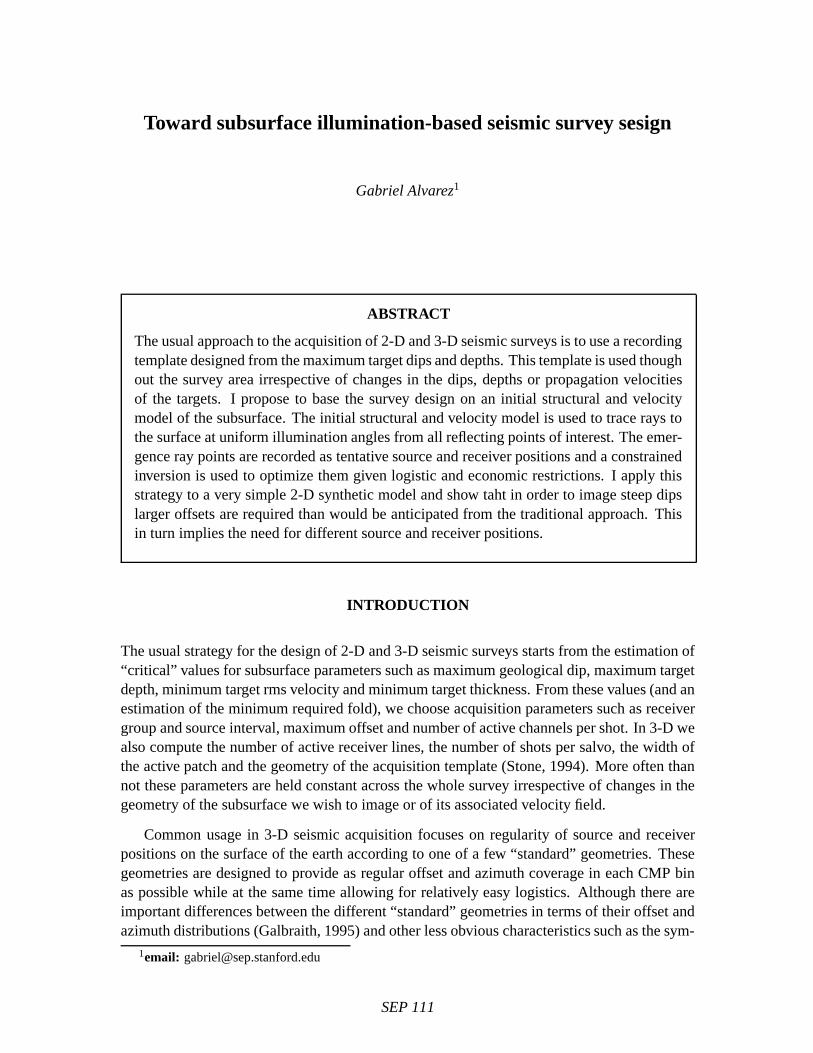
As a first test of the above ideas, I created a simple model shown in Figure 1. The model hasconstant velocity background of 3000 m/s.

−3 −2 −1 0 1 2 3

0

0.5

1

1.5

2

2.5

3

Horizontal Coordinate (km)

Dep

th (

km)

Figure 1: Simple model used to illustrate the proposed methodology. The background velocityis constant (3000 m/s) model1 [NR]

.Modeling with traditional parameters

In this case vmin = 3000 m/s, αmax = 90 and fmax = 50 Hz. Applying Equation 1 weget 1x = 30 m. The maximum depth of the target is 2000 m, so assuming an off-end cable(receivers to one side of the shot only) this will give about 67 receivers. This number rounds

SEP 111


up nicely to 72, which means an actual maximum offset of 2160 m (assuming that the firstreceiver is at an offset of 30 m). The shot interval is chosen as 1s = 1x = 30 m so that thefold of coverage (number of receivers per CMP) is 36. The trace length was chosen to be4 s. With these parameters I simulated acquisition using an analytical ray-tracing program.Obviously, we cannot expect to image the dips of the semicircular reflector up to 90 degreesbecause according to Equation 4 that would imply infinite aperture. The best we can do isimage the maximum dip for which the reflection time is less than or equal to the trace length.In this case, given the simple geometry of the reflector, a quick computation shows that for thezero offset trace this corresponds to shot positions ≈ ±6700 m. The corresponding maximumdip is ≈ 73 degrees.

The acquisition proceeds from left to right in Figure 1. When the shot is to the left of thesemicircle the longer offsets have shorter arrival times (from the semicircle) which means thatwe can actually achieve full fold at that point by extending the acquisition to the left by halfcable-length (1080 m). The first shot is therefore at -7780 m. When the shot is to the rightof the semicircle, on the other hand, longer offsets have longer arrival times and so we cannotexpect to have full fold at 6700 m. Any shot past that point will only contribute reflectionslonger than the trace length. In summary, with the standard approach (using the off-end cabledescribed above) in order to image the maximum dip we need shots between -7780 and 6700m. At 30 m shot interval this implies 483 shots.

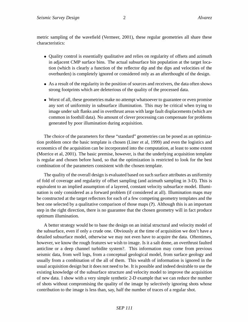
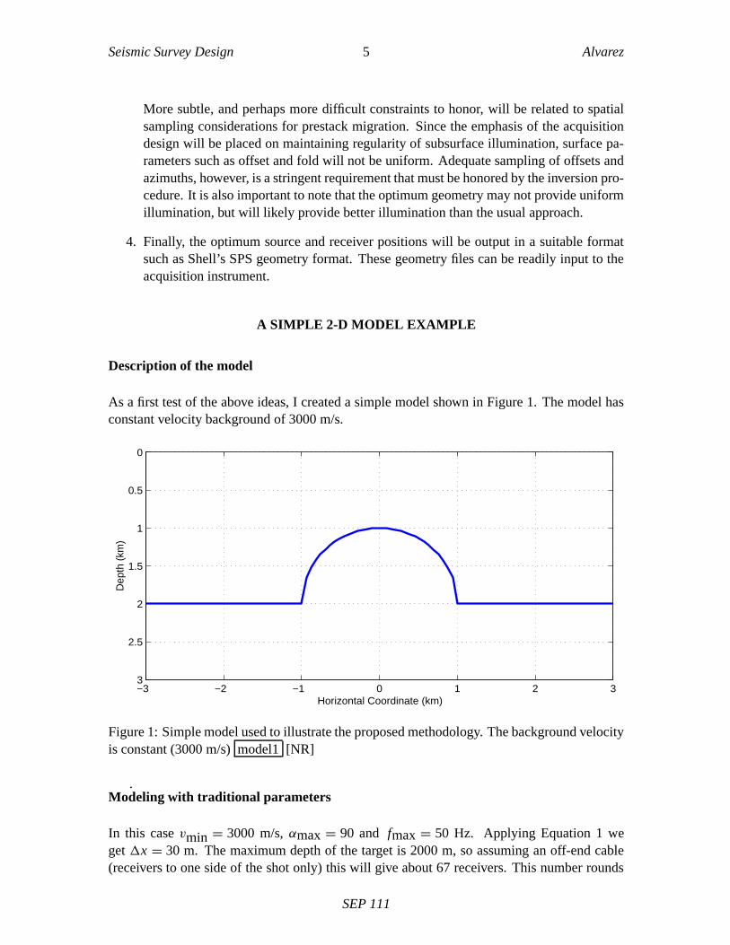
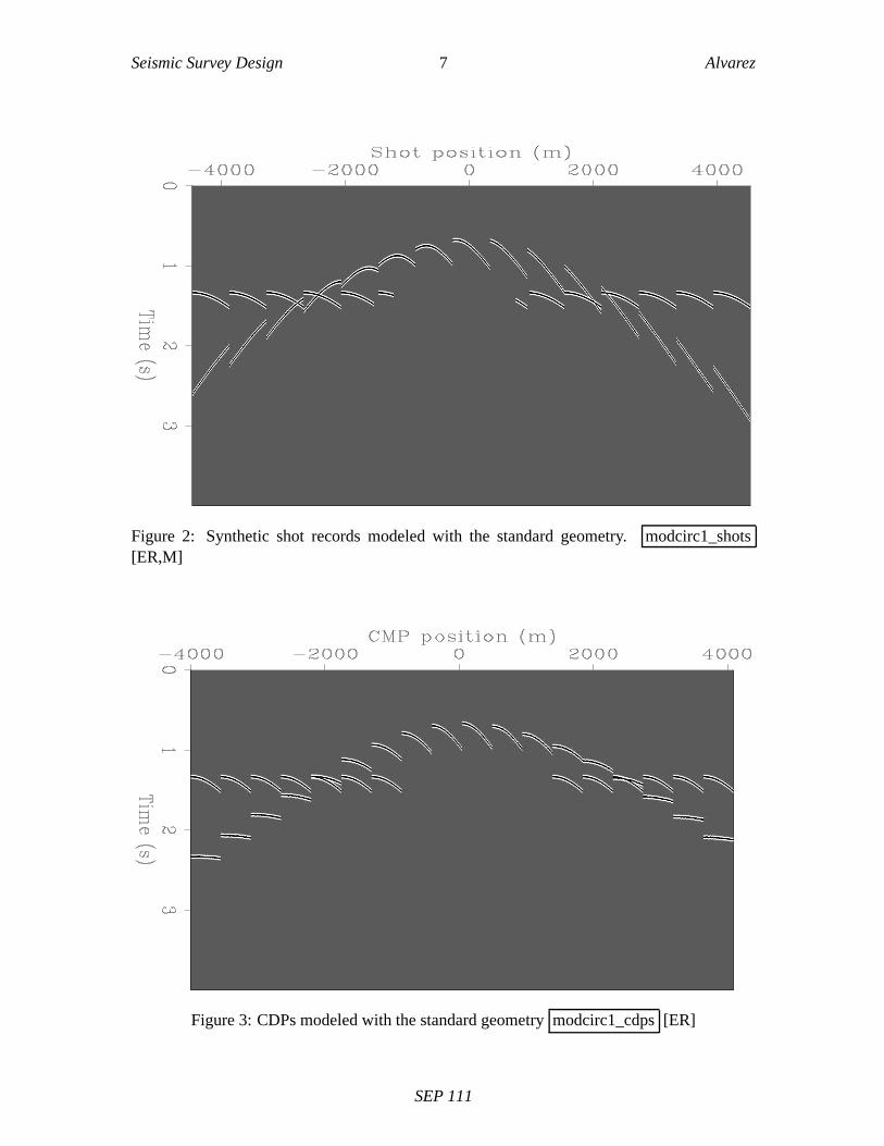
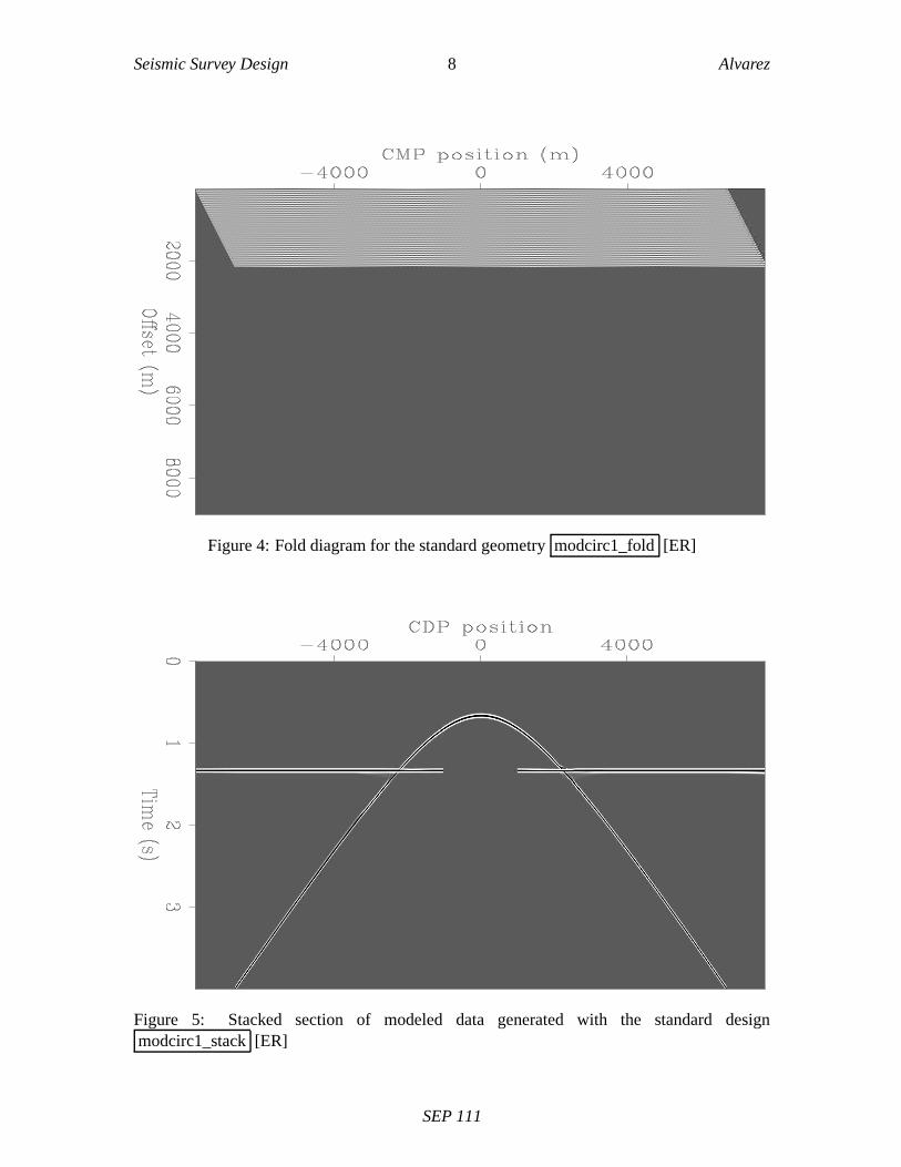
Figure 2 shows some of the modeled shot records. At both sides of the semicircle wesee two reflections coming from the flat and the semicircular reflector, whereas above thesemicircle only the reflection from the semicircular reflector is seen. Figure 3 shows someCMP gathers. Since the design is completely regular, the CMP’s are also regular. This isfurther illustrated in Figure 4 which shows the fold diagram. Note that we have full fold at-6700 m but not at 6700 m.

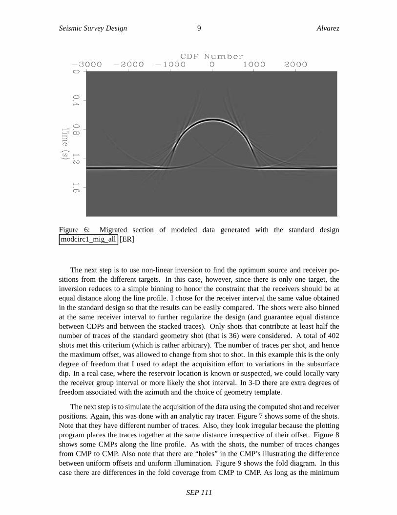
Figure 5 shows the stacked section. The noise at the intersection between the flat and thedipping reflections reflects the inherent difficult in picking a stacking velocity appropriate toboth (no DMO was applied). Finally, Figure 6 shows the post-stack migrated section using aStolt algorithm. As expected, dips in the semicircular reflector higher than 73 degrees werenot recovered.

Modeling with the proposed design

For the first step I used an analytic ray tracer to compute the surface emergence positions ofrays originating at equally-spaced reflection points along the reflector. These reflection pointswere taken every 18 m, corresponding to the CDP interval in the traditional design. For theflat reflector the number of pairs of rays originating at each point was kept equal to the foldin the standard design. The rays correspond to a uniform increase in reflection aperture angleand therefore will not correspond to uniform offsets in a CMP gather. In the semicircle thenumber of rays was increased as a function of the reflector dip, so that where the dips are largermore rays were generated. The maximum offset was not constrained except for the obviousrequirement that any reflection time were less than the chosen trace length.

SEP 111


Figure 2: Synthetic shot records modeled with the standard geometry. modcirc1_shots[ER,M]

Figure 3: CDPs modeled with the standard geometry modcirc1_cdps [ER]

SEP 111


Figure 4: Fold diagram for the standard geometry modcirc1_fold [ER]

Figure 5: Stacked section of modeled data generated with the standard designmodcirc1_stack [ER]

SEP 111


Figure 6: Migrated section of modeled data generated with the standard designmodcirc1_mig_all [ER]

The next step is to use non-linear inversion to find the optimum source and receiver po-sitions from the different targets. In this case, however, since there is only one target, theinversion reduces to a simple binning to honor the constraint that the receivers should be atequal distance along the line profile. I chose for the receiver interval the same value obtainedin the standard design so that the results can be easily compared. The shots were also binnedat the same receiver interval to further regularize the design (and guarantee equal distancebetween CDPs and between the stacked traces). Only shots that contribute at least half thenumber of traces of the standard geometry shot (that is 36) were considered. A total of 402shots met this criterium (which is rather arbitrary). The number of traces per shot, and hencethe maximum offset, was allowed to change from shot to shot. In this example this is the onlydegree of freedom that I used to adapt the acquisition effort to variations in the subsurfacedip. In a real case, where the reservoir location is known or suspected, we could locally varythe receiver group interval or more likely the shot interval. In 3-D there are extra degrees offreedom associated with the azimuth and the choice of geometry template.

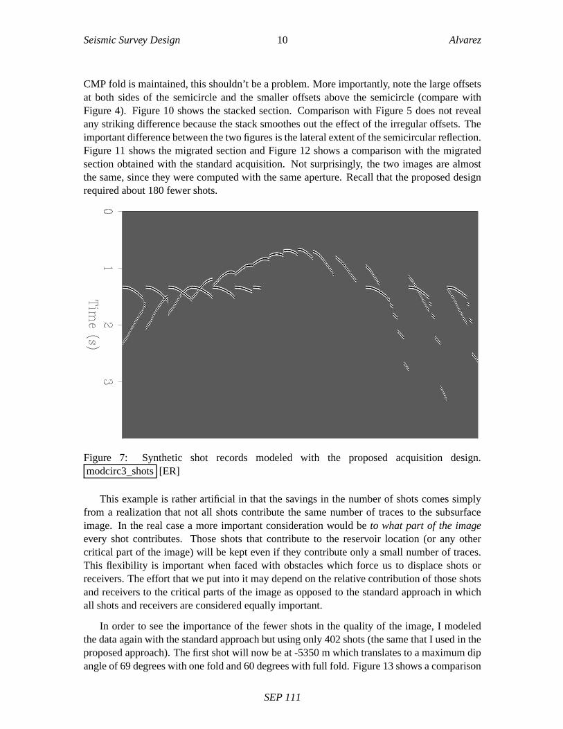
The next step is to simulate the acquisition of the data using the computed shot and receiverpositions. Again, this was done with an analytic ray tracer. Figure 7 shows some of the shots.Note that they have different number of traces. Also, they look irregular because the plottingprogram places the traces together at the same distance irrespective of their offset. Figure 8shows some CMPs along the line profile. As with the shots, the number of traces changesfrom CMP to CMP. Also note that there are “holes” in the CMP’s illustrating the differencebetween uniform offsets and uniform illumination. Figure 9 shows the fold diagram. In thiscase there are differences in the fold coverage from CMP to CMP. As long as the minimum

SEP 111


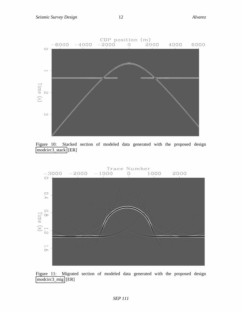
CMP fold is maintained, this shouldn’t be a problem. More importantly, note the large offsetsat both sides of the semicircle and the smaller offsets above the semicircle (compare withFigure 4). Figure 10 shows the stacked section. Comparison with Figure 5 does not revealany striking difference because the stack smoothes out the effect of the irregular offsets. Theimportant difference between the two figures is the lateral extent of the semicircular reflection.Figure 11 shows the migrated section and Figure 12 shows a comparison with the migratedsection obtained with the standard acquisition. Not surprisingly, the two images are almostthe same, since they were computed with the same aperture. Recall that the proposed designrequired about 180 fewer shots.

Figure 7: Synthetic shot records modeled with the proposed acquisition design.modcirc3_shots [ER]

This example is rather artificial in that the savings in the number of shots comes simplyfrom a realization that not all shots contribute the same number of traces to the subsurfaceimage. In the real case a more important consideration would be to what part of the imageevery shot contributes. Those shots that contribute to the reservoir location (or any othercritical part of the image) will be kept even if they contribute only a small number of traces.This flexibility is important when faced with obstacles which force us to displace shots orreceivers. The effort that we put into it may depend on the relative contribution of those shotsand receivers to the critical parts of the image as opposed to the standard approach in whichall shots and receivers are considered equally important.

In order to see the importance of the fewer shots in the quality of the image, I modeledthe data again with the standard approach but using only 402 shots (the same that I used in theproposed approach). The first shot will now be at -5350 m which translates to a maximum dipangle of 69 degrees with one fold and 60 degrees with full fold. Figure 13 shows a comparison

SEP 111


Figure 8: Selected CDPs modeled with the proposed methodology. modcirc3_cdps [ER]

Figure 9: Fold diagram for the proposed methodology modcirc3_fold [ER]

SEP 111


Figure 10: Stacked section of modeled data generated with the proposed designmodcirc3_stack [ER]

Figure 11: Migrated section of modeled data generated with the proposed designmodcirc3_mig [ER]

SEP 111


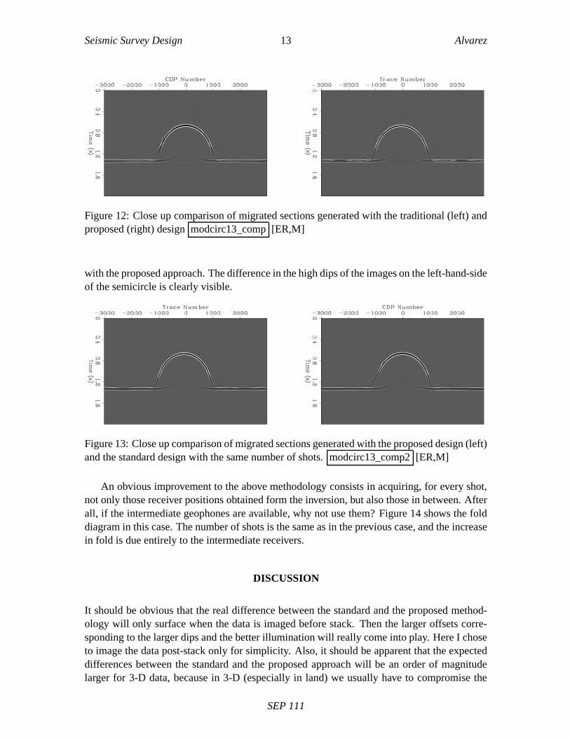
Figure 12: Close up comparison of migrated sections generated with the traditional (left) andproposed (right) design modcirc13_comp [ER,M]

with the proposed approach. The difference in the high dips of the images on the left-hand-sideof the semicircle is clearly visible.

Figure 13: Close up comparison of migrated sections generated with the proposed design (left)and the standard design with the same number of shots. modcirc13_comp2 [ER,M]

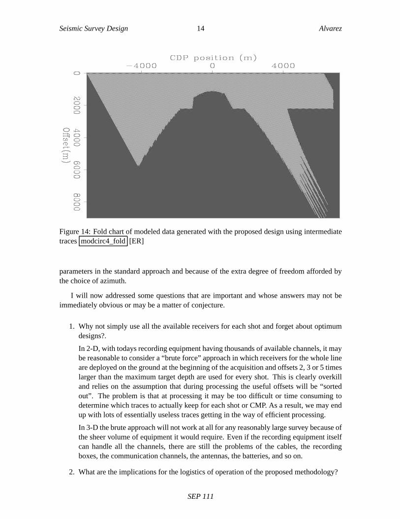
An obvious improvement to the above methodology consists in acquiring, for every shot,not only those receiver positions obtained form the inversion, but also those in between. Afterall, if the intermediate geophones are available, why not use them? Figure 14 shows the folddiagram in this case. The number of shots is the same as in the previous case, and the increasein fold is due entirely to the intermediate receivers.

DISCUSSION

It should be obvious that the real difference between the standard and the proposed method-ology will only surface when the data is imaged before stack. Then the larger offsets corre-sponding to the larger dips and the better illumination will really come into play. Here I choseto image the data post-stack only for simplicity. Also, it should be apparent that the expecteddifferences between the standard and the proposed approach will be an order of magnitudelarger for 3-D data, because in 3-D (especially in land) we usually have to compromise the

SEP 111


Figure 14: Fold chart of modeled data generated with the proposed design using intermediatetraces modcirc4_fold [ER]

parameters in the standard approach and because of the extra degree of freedom afforded bythe choice of azimuth.

I will now addressed some questions that are important and whose answers may not beimmediately obvious or may be a matter of conjecture.

1. Why not simply use all the available receivers for each shot and forget about optimumdesigns?.

In 2-D, with todays recording equipment having thousands of available channels, it maybe reasonable to consider a “brute force” approach in which receivers for the whole lineare deployed on the ground at the beginning of the acquisition and offsets 2, 3 or 5 timeslarger than the maximum target depth are used for every shot. This is clearly overkilland relies on the assumption that during processing the useful offsets will be “sortedout”. The problem is that at processing it may be too difficult or time consuming todetermine which traces to actually keep for each shot or CMP. As a result, we may endup with lots of essentially useless traces getting in the way of efficient processing.

In 3-D the brute approach will not work at all for any reasonably large survey because ofthe sheer volume of equipment it would require. Even if the recording equipment itselfcan handle all the channels, there are still the problems of the cables, the recordingboxes, the communication channels, the antennas, the batteries, and so on.

2. What are the implications for the logistics of operation of the proposed methodology?

SEP 111


The logistics of operation do not need to be strongly affected since the receivers willbe deployed as usual and the recording equipment will electronically connect and dis-connect the required receiver stations for each shot based on the information of thegeometry (SPS) files. Thus, the fact that the template may change from shot to shot (orfrom salvo to salvo in 3-D) is not a negative logistics issue.

3. Why acquire the intermediate traces?. If we already computed the optimum positionsfor sources and receivers so as to have “perfect” illumination what valuable informationcan there be in the intermediate traces?. Why go to all the trouble of finding optimumreceiver positions if we are going to use the intermediate receivers as well?.

The intermediate traces, although possibly contributing redundant illumination, will beuseful for random noise suppression, for velocity computations and for offset samplingnecessary for prestack migration. Besides they will not require any significant extraacquisition effort.

4. What are the implications of the non-uniform offset distribution for prestack migrationof the data?. Can we guarantee that there will not be spatial aliasing in the offset dimen-sion?

This is an open question for which I don’t have a definitive answer yet. The idea isto include the sampling requirements for prestack migration as constraints to the inver-sion process, so that additional receiver or shot positions be considered to satisfy thatconstraint. The details of how to do that, especially in 3-D, is an interesting researchissue.

5. What would be the situation for 3-D acquisition?

For 3-D the situation is more challenging but also much more interesting and useful.We have now not only the degree of freedom afforded by the choice of offsets but by thechoice of azimuths as well. Besides, the basic geometry template can also be considereda design parameter that (unlike common practice) can change spatially. The inversionprocess will be extremely difficult and strongly non-unique.

A more philosophical question, but one that has an important meaning is: What kind ofdata would we regard as ideal from the point of view of imaging? That is, assuming that wehave no logistic or economic restriction whatsoever (except that the data can only be acquiredat the surface), what would be the ideal data?

For the standard approach, some characteristics of this ideal data immediately come tomind: data in a very fine regular grid with a very large aperture. This is fine, and wouldprovide us with a good image. I believe, however, that the ideal data would be data withvery fine, regular subsurface illumination, with aperture being a function of the illuminationrequirements.

That subsurface illumination is an important attribute of a good design is not new. Infact most commercial software for seismic survey design offer an option to trace rays intothe subsurface for a given design to produce illumination maps of the targets of interest. The

SEP 111


maps obtained with different designs are compared and this information taken into accountwhen deciding what the best design is or changes may be introduced to the designs and theprocess iterated. This is an example of the forward problem. What I propose is to base thesurvey design on the inverse problem: start with an initial model and choose the layout ofsources and receivers to obtain optimum illumination.

SUMMARY AND CONCLUSIONS

Using all the available subsurface information to design the acquisition parameters of newseismic surveys in a given area seems like the sensible thing to do. Common practice, however,uses only maximum and minimum values of targets velocities, dips and depths. Starting froma subsurface model may seem to bias the acquisition, but we have to keep in mind that by notusing any model we are in fact imposing a model of flat layers and constant velocity.

The real impact and usefulness of this methodology arises in 3-D land seismic acquisitionwhere the cost of the surveys oftentimes requires the design to be a compromise of the differentsubsurface parameters in different parts of the survey. The design is then kept constant forthe whole area. By adapting the acquisition effort locally to the imaging demands of thesubsurface we could in principle acquire better data at the same cost or perhaps even cheaper.

It is all too common in 3-D land data that significant obstacles force us to deviate fromthe original design. The common practice is to displace shots and receivers to alternativepositions chosen to maintain, as much as possible, the uniformity of fold and the regularity ofoffsets and azimuth distribution. All sources and receivers are considered equally importantto the subsurface image, which is probably not a good idea in general. The presence of largeobstacles can be incorporated into the design procedure and alternative source and receiverlocations chosen to optimize the regularity of the illumination as opposed to the regularity offold, offset or azimuth distributions as is standard practice. It may very well happen that someshots in the excluded area turn out not to contribute significantly to the critical parts of theimage and so can be simply ignored if they are difficult to replace. On the other hand, it mayturn out that those shots are critical and then there are concrete reasons to make a strongereffort to acquire them.

In conclusion, we should be able to use all the available information when designing theacquisition of a new survey and make decisions with as much information as possible. Shiftingthe emphasis from surface parameters (fold, offsets and azimuths) to subsurface parameters(illumination) is a step in the right direction.

THE WAY AHEAD

Clearly, the methodology described in this paper is only weakly supported by the simple 2-Dexample presented here. The challenge lies in the implementation of the non-linear inver-sion process capable of computing the optimum source and receiver positions given all thegeophysical, logistical and financial constraints for 3-D data.

SEP 111


The sensitivity of the acquisition geometry to the accuracy of the initial structural andvelocity model is also clearly an important issue to be analyzed in detail. Extensive researchwill have to be done before clear guidelines can be established in that respect.

REFERENCES

Cain, G., Cambois, G., Gehin, M., Hall, R. 1998. Reducing risk in seismic acquisition andinteropretation of complex targets using a Gocad-based 3D modeling tool. Expanded Ab-stracts. pp 2072-2075. Society of Exploration Geophysicists.

Galbraith, M., 1995, Land 3-D survey design by computer. Australian Society of ExplorationGephysicists 25, 71-78.

Liner, C., Underwood, W., Gobeli, R., 1999. 3-D seismic survvey design as an optimizationproblem. The Leading Edge of Eploration. September 1999, pp. 1054-1060. Society ofExploration Geophysicists.

Morrice, D., Kenyoun, A., Beckett, C., 2001. Optimzing operations in 3-D land seismic sur-veys. Geophyisics 66, 1818-1826.

Stone, D. G., 1994, Designing Seismic Surveys in two and three diensions: Society of Explo-ration Geophysicists.

Vermeer, G. J., 2001, Fundamentals of 3-D seismic survey design. PhD thesis, Delft Universityof Technology.

SEP 111

Documents

Toward subsurface illumination-based seismic …sep Survey Design 2 Alvarez metric sampling of the waveﬁeld (Vermeer, 2001), these regular geometries all share these characteristics: