Towards a Theory of Trade Finance∗

Tim Schmidt-Eisenlohr†

University of Oxford

First version: December 2009

This version: March 2011

Abstract

Shipping goods internationally is risky and takes time. To allocate risk and to

finance the time gap between production and sale, a range of payment contracts is

utilized. I study the optimal choice between these payment contracts considering

one shot transactions, repeated transactions and implications for trade. The equi-

librium contract is determined by financial market characteristics and contracting

environments in both the source and the destination country. Trade increases in

enforcement probabilities and decreases in financing costs proportional to the time

needed for trade. Empirical results from gravity regressions are in line with the

model, highly significant and economically relevant.

Keywords : trade finance, payment contracts, trade patterns, distance interaction

JEL-Codes : F12, F3, G21, G32

∗I am grateful to Giancarlo Corsetti, Andrew Bernard, Russell Cooper and Omar Licandro for con-stant advice. I would also like to thank Agnes Benassy-Quere, Jeffrey Bergstrand, Jonathan Eaton,Oliver Hart, Sebastian Krautheim, Giordano Mion, Friederike Niepmann, Emanuel Ornelas, StephenRedding, Vincent Rebeyrol, Tony Venables and Adrian Wood, as well as participants at the CESifo AreaConference on Global Economy, Verein fur Socialpolitik Annual Meeting, the European Workshop inMacroeconomics, ESNIE 2010, RIEF 2010, the De Nederlandsche Bank research seminar, OxCarre andthe Royal Economic Society PhD Presentation Meeting. This is a revised version of EUI Working Paper2009/43 (December 2009). All remaining errors are mine. I acknowledge financial support from CESifoand the ESRC (Grant No RES -060-25-0033).†Centre for Business Taxation, Saıd Business School, University of Oxford, Park End Street, Oxford,

OX1 1HP, UK; Tim.Schmidt-Eisenlohr@sbs.ox.ac.uk

1 Introduction

Shipping goods internationally is risky and takes time. Therefore, trading partners not

only have to agree on the specification and the price of a good, but also need to decide on

the timing of payments. To allocate risk and to finance the time gap between production

and sale, a range of different payment contracts is utilized. These can be broadly classified

into exporter finance (Open Account), importer finance (Cash in Advance) and bank

finance (Letter of Credit).1

In this paper, I study the optimal choice between these three types of payment con-

tracts, considering one shot transactions, repeated transactions and implications for trade.

The equilibrium contract is determined by financial market characteristics and contract-

ing environments in the source and the destination country. A transaction should, in

general, be financed by the firm in the country with the lower financing costs and the

weaker contract enforcement. This minimizes interest rate costs and the probability that

the trading partner which did not pre-finance the transaction defaults on its contractual

obligations. When two firms in countries with weak contract enforcement trade with

each other, bank finance (Letter of Credit) is most useful as it resolves the moral hazard

problem of defaulting.2 Repeated transactions are an alternative way to reduce trade

risk as the continuation value of a trading relationship gives firms an additional incentive

to fulfill contracts. Therefore, they make exporter finance (Open Account) and importer

finance (Cash in Advance) relatively more attractive compared to bank finance (Letter

of Credit).

Through the payment contract choice, financing costs and contracting environments

in the source and the destination country interact to shape trade finance costs. These are

variable trade costs proportional to the value of goods exported, isomorphic to the iceberg

trade cost formulation as introduced by Samuelson (1954). Being an obstacle to trade,

trade finance costs affect trade patterns. Exports increase in enforcement probabilities

and decrease in financing costs. The latter effect is the larger, the longer it takes from

1According to survey evidence reported in IMF (2009), 42-48 percent of transactions are done throughOpen Account, which corresponds to pure exporter financing. Cash in Advance, which represents pureimporter financing, accounts for 19-22 percent and bank intermediated transactions account for the restof transactions. The wide use of different working capital practices is also documented by Wagner Ricciand Morrison (1996), who surveyed Fortune 200 companies.

2I also study the case of intermediate type contracts with a partial pre-payment. They are a meansto reduce financing costs, but cannot resolve the moral hazard problem of the importer.

2

production to sale.

The availability of different payment contracts can be beneficial if financial conditions

change. Suppose, for example, a country experiences a financial crisis that leads to a rise

in interest rates. Then, a payment contract switch can limit adverse effects by moving the

financing activity to the country of the trading partner. This is not possible if financial

conditions in both countries deteriorate at the same time. Therefore, multilateral crises

should have a larger impact on trade flows than national crises.

I illustrate in a numerical example that the choice between payment contracts is

economically relevant. In a baseline calibration, export quantities of a country decrease

by up to 20.1 percent, when all firms are forced to use exporter finance (Open Account)

only.

In the empirical part of the paper, I test key predictions of the model using a panel

of bilateral trade flows. I run gravity regressions including interaction terms between

distance and financing costs in the source and the destination country to identify the

effect of trade finance on trade flows. I find that two countries trade less with each other

if their financing costs are higher. As predicted, this effect is the larger, the more time is

needed for trade.3 Results are highly significant and economically relevant.

The paper is related to two strands of theoretical literature. First, there is a large

number of papers that study the use of trade credit between firms. Trade credit usually

refers to downstream lending between firms in a supply chain, both inside a country

and across borders. International trade credit therefore corresponds to one of the three

payment contracts considered in this paper, namely Open Account. The literature has

concentrated on the relationship of two firms inside a country and has studied under

which circumstances trade credit is used as a substitute for bank credit and what the

underlying costs and benefits are.4 In this paper, the focus is instead on the trade-off

between financing costs and contracting environments in different countries to optimally

finance trade transactions. The analysis abstracts from any frictions that could imply a

wedge between bank and firm finance inside a country, which is the central issue studied

in the trade credit literature.

3As no direct time to trade data is available, I use geographical distance as a proxy for the timeneeded for trade.

4See Biais and Gollier (1997), Petersen and Rajan (1997), Wilner (2000), Burkart and Ellingsen(2004), Cunat (2007) and Giannetti et al. (forthcoming).

3

Second, there are theoretical papers that have considered the relationship between

financial market conditions and international trade. Kletzer and Bardhan (1987) show

how sovereign default risk and credit market imperfections can result in differences in

interest rates and tightness of credit rationing in equilibrium, respectively, and create

a comparative advantage. In Matsuyama (2005), the share of revenues an entrepreneur

can pledge towards wage payments differs between countries leading to a comparative

advantage.5 Chaney (2005) develops a theoretical model analyzing financial constraints

in a heterogeneous firms trade model based on Melitz (2003). Firms have to finance

their fixed entry cost into foreign markets through own liquidity and domestic operating

profits. Liquidity is introduced as a second type of heterogeneity. He derives conditions

on productivity and liquidity under which a firm exports. Manova (2008b) extends this

model to a setting where also export volumes can be affected by financial constraints.

In Chaney (2005) and Manova (2008b) only domestic financial market conditions in the

form of financial constraints are relevant for the export decisions of firms. In particular,

there is no role for financial market conditions and the contracting environment in the

destination country and for the costs of trade finance.

While there is no paper that formally studies the choice of payment contracts for

trade finance, some other aspects of trade finance are discussed in policy papers.6 Fi-

nally, my paper relates to two, more recent contributions on theoretical aspects of trade

finance. Ahn (2010) studies why international transactions might get relatively riskier

and why credit supply constraints might affect international trade loans relatively more

in a financial crisis. Olsen (2010) elaborates on the idea also discussed in this paper, that

enforcement between banks might be easier than between two trading partners, as the

former interact more frequently.

There is a large empirical literature that has provided evidence on the relationship be-

tween the financial development of a country and the sectoral concentration of its exports.

5The broader issue of institutional constraints, trade and outsourcing has been studied extensively.Recent contributions include Nunn (2007), Levchenko (2007) and Antras et al. (2009). For a survey seeHelpman (2006).

6Menichini (2009) discusses inter-firm trade finance. She emphasizes the possibility that shocks arepropagated through credit chains. Furthermore, she argues that the use of trade finance might berestricted if institutions like contract enforcement and bankruptcy laws are not sufficiently developed.Ellingsen and Vlachos (2009) develop a model of trade credit in a liquidity crisis. They show that inthe presence of liquidity hoarding, targeted support of trade finance might be better than increasingthe general supply of credit in an economy. Evidence on firm level trade finance of African exporters isdocumented by Humphrey (2009).

4

The general finding is that financial development creates a comparative advantage in in-

dustries that are more financially dependent and in which assets are less tangible.7 The

question whether financial constraints affect the decision to export and export volumes is

the focus of a growing number of papers. This literature has so far been inconclusive on

the question of causality from financial conditions to exporting decisions as endogeneity

remains a key concern.8 Amiti and Weinstein (2009) resolve the endogeneity problem

using Japanese matched firm-bank data. They identify a bank-firm trade finance channel

and find that it accounts for about one third of the decline in exports during the crisis

in Japan in the 1990s.9

Several authors have studied factors that led to the large drop in international trade

in the recent financial crisis. Besides demand side and composition effects (see Eaton et

al. (2009), Levchenko et al. (2009), Behrens et al. (2010), Yi et al. (2010)) and inventory

adjustments (Alessandria et al. (2010)), some research also provides evidence for the role

of financial factors. Berman and Martin (2009) analyze how a financial crisis affects

trade and find that its effects are stronger and longer lasting for African than for other

countries. They find furthermore that African countries with a higher than median trade

credit over exports ratio are hit harder. Bricongne et al. (2010) study french firm level

data. While they find effects of credit constraints at the firm level, they argue that, as

the share of constrained firms is small, aggregate effects through this channel are limited.

Chor and Manova (2010) study US imports and find a negative relationship between

interbank rates in a country and its exports in more financially dependent sectors during

the recent crisis. Using data from a private trade insurance company, van der Veer (2010)

estimates that about 5 to 9 percent of the drop in world exports was due to a reduction

in trade insurance coverage. In a recent paper, Paravisini et al. (2010) use Peruvian bank

credit data at the firm-level and find that credit supply shocks can explain 15 percent of

the decline in exports during the financial crisis.

The empirical part of the paper differs from the existing literature in three aspects.

First, motivated by the theoretical results, I consider financing costs both in the source

7See Beck (2002), Beck (2003), and Manova (2008b).8Using firm level data, this question has been addressed for example by Greenaway et al. (2007),

Muuls (2008), and Berman and Hericourt (2010). Manova (2008a) and Manova (2008b) studies creditconstraints using sectoral level data.

9The effects of previous crises on trade have also been studied by Ronci (2004) and Iacovone andZavacka (2009).

5

and the destination country.10 Second, a financial market efficiency measure, the net

interest margin, is used, to study the effects of financing costs on trade flows.11 Finally, a

distance interaction is employed to test for an effect of financial conditions proportional

to the time needed for trade.12

The rest of the paper is organized as follows. Section 2 introduces a model of pay-

ment contracts. Section 3 extends the analysis to repeated contracts. Section 4 sets the

model into a standard intra-industry trade framework, derives implications for trade pat-

terns, evaluates the quantitative importance of payment contracts and discusses payment

contract switches. Section 5 presents empirical results. Section 6 concludes.

2 Payment Contracts

To allocate risk and to finance the time gap between the production and the sale of a

product, a wide range of payment contracts is utilized. I study the optimal choice of

trading partners between these contracts, considering three representative types. These

are Open Account (exporter finance), Cash in Advance (importer finance) and Letter

of Credit (bank finance). Furthermore, an analysis of an intermediate type contract,

combining exporter finance and importer finance, is provided.

The choice between different payment contracts is relevant for two reasons. First, the

time gap between the production of goods and the realization of sales revenues is longer

for international trade than for domestic sales. As Hummels (2001) reports, physical

transport times can be substantial in international trade, in particular, when goods are

transported by sea. Additionally, Djankov et al. (2010) document that formal procedures

necessary for international trade transactions can be extensive, implying a delay from the

factory gate to the means of transportation as well as at the border of the importer. Amiti

10An exception is Manova (2008b), who, in a recent revision mentions results from a regression withdestination country variables. She finds effects about one third of the size of the exporter variables.

11While the net interest rate margin has not been used in this context, empirical work by Chor andManova (2010) and Korinek et al. (2010) studies the relationship of trade flows with interbank rates andthe US high yield spread during the recent financial crisis, respectively.

12As discussed in detail in Section 5, the distance interaction provides a new and direct identificationof variable trade costs due to financing requirements. In this, my results contribute to the literatureestimating trade costs. See among others Eaton and Kortum (2002), Anderson and van Wincoop (2003),Hummels (2007), Jacks et al. (2008) and Irarrazabal et al. (2010). In contemporaneous empirical workon the financial crisis, Paravisini et al. (2010) include an interaction term between distance and creditsupply of a firm but do not find any significant effects.

6

and Weinstein (2009) calculate that these two causes of delay add up to approximately

two months for the median case.13 This implies that working capital requirements for

international trade are larger than for domestic sales.

Second, it is more difficult to enforce contracts across borders. This can be due to

differences in legal systems or working languages and a limited willingness of governments

to enforce international contracts to the same degree as national ones. Whereas domestic

sales naturally take place in a common contracting environment, international trade in

general does not. Furthermore, in international trade, a firm might not have a permanent

representation in the country of the trading partner, making litigation more difficult and

costly. Consequently, international trade is more risky and the allocation of risk more

important.

2.1 Setup

Suppose there is one exporter and one importer. The exporter can make a take it or

leave it offer to the importer. There are two points in time. At t = 0 firms agree on a

payment contract and the exporter can produce and send goods off to the destination

country. After t time units, goods can arrive and sales revenues can be realized. Denote

production costs by K and revenues by R. Assume further that R > K.

There are two imperfections in the economy. First, markets to finance international

trade transactions are segmented and efficiencies of financial intermediaries differ across

countries. As a result the interest rate a firm faces depends on its location. Second, there

is limited enforcement of contracts, modeled as an exogenous country-specific probability

that a contract will be enforced, in case that a firm does not want to fulfill it voluntarily.14

Under Cash in Advance, it is the probability that the exporter is forced to deliver the

goods after receiving the payment. Under Open Account, it is the probability that an

importer has to pay the agreed price for the goods after receiving and selling them.15

13The median numbers they quote are 21 days from factory to ship in the exporting country and 23days from the ship to the warehouse in the importing country. Average sea transport time to the USaccounts for another 20 days in their calculation.

14This captures the reduced form of an enforcement game played between the importer and the ex-porter, which is affected by the legal institutions of the two countries. This could be extended to amodel in which firms choose their legal expenditures to achieve or prevent enforcement. In that case theenforcement probability would change with the value at stake and there would be an explicit role forfirm heterogeneity.

15For simplicity these two enforcement probabilities are assumed to be equal. It would be an interesting

7

Furthermore, assume that the amount to be paid by the importer for the goods traded

cannot exceed their total value at market prices.16 In the following, I formally describe

the three financing forms and derive conditions under which each of them is chosen. Let

λ and r denote the enforcement probability and the interest rate in the source country,

respectively. Variables for the destination country are marked with asterisks.

2.2 Cash in Advance, Open Account and Letter of Credit

Cash in Advance Under Cash in Advance (CIA) the importer first pays the amount

CCIA to the exporter. With probability λ the contract is enforced. In this case the

exporter produces the goods at cost K and delivers them to the importer, who sells them

for R. The exporter makes a take it or leave it offer and has to respect the limited value

of contract and the importer participation constraint:

maxC

E[ΠCIAE

]= CCIA − λK, (1)

s.t. CCIA ≤ R, (limited value of contract) (2)

and E[ΠCIAI

]= λR− (1 + r∗)tCCIA ≥ 0. (participation constraint importer) (3)

Under CIA, the trade transaction is financed by the importer. Her participation con-

straint requires that, taking the default probability into account, her expected profits are

non-negative. As the exporter has all negotiation power and the limited value of contract

constraint never binds under CIA, the participation constraint binds under the optimal

contract. The optimal payment CCIA and optimal expected profits of the exporter are:

CCIA =λ

(1 + r∗)tR, E

[ΠCIAE

]=

λ

(1 + r∗)tR− λK. (4)

Note that the optimal payment CCIA is proportional to λ, i.e. the payment is discounted

by the probability of non-delivery by the exporter. Despite the fact that there are strictly

extension to consider an asymmetry here. This could be rationalized by the difference between the in-kind nature of Open Account and the cash nature of Cash in Advance. For a formalization of thisargument see Burkart and Ellingsen (2004).

16This limited value of contract assumption corresponds to a special case of a model with wealthconstraints, where the wealth of the importer is assumed to be zero. In principle, the model could besolved for non-zero wealth levels, but the analysis would be substantially less tractable. For details seeAppendix B.

8

positive gains from trade, under CIA, production and delivery only take place with prob-

ability λ.

Open Account Under Open Account (OA), the exporter first produces the goods at

cost K and delivers them to the importer. Then, the importer sells the goods for R.

With probability λ∗ the contract is enforced and the importer pays the amount COA to

the exporter. The maximization problem of the exporter is:

maxC

E[ΠOAE

]=

1

(1 + r)t(λ∗COA −K(1 + r)t), (5)

s.t. COA ≤ R, (limited value of contract) (6)

and E[ΠOAI

]=

1

(1 + r∗)t(R− λ∗COA) ≥ 0, (participation constraint importer) (7)

assuming that the exporter and importer discount profits with their local interest rates.17

Now, the exporter pre-finances the trade transaction. Due to the limited value of contract

constraint the maximum payment COA that is contractible is R. If λ∗ < 1 this implies

that the exporter is not able to extract all rents from the importer, who consequently has

positive expected profits. The optimal payment amount COA and the optimal discounted

expected exporter profits can be derived as:

COA = R, E[ΠOAE

]=

λ∗

(1 + r)tR−K. (8)

Letter of Credit Under a Letter of Credit (LC), both the exporter and the importer

pre-finance the transaction and incur costs due to interest rate payments. The contract

enforcement problem is resolved by an indirect transaction with banks as intermediaries.

The importer does not directly pay the exporter, but first pays the amount CLC to a

local bank.18 The bank cooperates with a bank in the country of the exporter. The latter

guarantees payment upon proof of delivery. Under the assumption of no default at the

bank level and perfect third party verifiability, this completely resolves the enforcement

17To compare profits between CIA and OA they have to be discounted to the same time period.18Often firms do not actually pay the amount to the bank in cash, but receive a credit for the amount

and period of the LC against a fee. As I assume perfect enforcement in the domestic financial market,the two are equivalent as long as firms discount at the lending rate.

9

problem at the individual contract level.19 The maximization problem of the exporter is:

maxC

E[ΠLCE

]=

1

(1 + r)t(CLC −K(1 + r)t), (9)

s.t. CLC ≤ R, (limited value of contract) (10)

and E[ΠLCI

]=

R

(1 + r∗)t− CLC ≥ 0. (participation constraint importer) (11)

In the case of LC, the limited value of contract constraint never binds while the partici-

pation constraint of the importer is binding. The optimal payment CLC and discounted

expected exporter profits are:

CLC =R

(1 + r∗)t, E

[ΠLCE

]=

1

[(1 + r)(1 + r∗)]tR−K. (12)

Note that, as pre-financing takes place on both sides, the interest rates from both markets

affect profits. As enforcement risk is completely resolved, profits are independent of the

enforcement parameters λ and λ∗.

Comparison CIA, OA and LC The four parameters r, r∗, λ, λ∗ together with the

production cost K and sales revenue R determine a unique ordering of the different

payment forms as stated below:20

Proposition 1 Suppose R and K exogenously given. Then, the optimal choice of pay-

ment contract is uniquely determined by the following three conditions:

i) OA ≺ CIA⇐⇒ K

R<

λ∗(1 + r∗)t − λ(1 + r)t

[(1 + r)(1 + r∗)]t(1− λ),

ii) OA ≺ LC ⇐⇒ λ∗(1 + r∗)t > 1,

iii) LC ≺ CIA⇐⇒ K

R<

1− λ(1 + r)t

[(1 + r)(1 + r∗)]t(1− λ).

Proof. Follows directly from comparing expected discounted profits from Equations 4,

8 and 12.

19It is conceivable that full enforcement at the banking level is more likely than at the firm level. Asbanks tend to have more long-term relationships, reputation building and repeated transactions easeenforcement between them. Recently, this idea has been looked at in detail by Olsen (2010).

20Assume for now K and R to be exogenous and the same for all payment contracts. When introducingan explicit demand, different payment contracts imply different optimal levels of K and R.

10

Several predictions, which could be tested with transaction level data, can be derived:

Proposition 2 The usage of

i) CIA increases in λ, r and t and decreases in λ∗ and r∗.

ii) OA increases in λ∗, r∗ and t and decreases in λ and r.

iii) LC decreases in r, r∗, λ, λ∗ and t.

Proof. Follows from comparing Equations 4, 8 and 12.

2.3 Intermediate Type Contracts

An intermediate type contract refers to the case when part of the payment is done in

advance whereas the remainder is payed after delivery. Let φ ∈ (0, 1) denote the share of

advance payment, i.e. C0 = φC. Such a contract could be motivated by the possibility to

reduce moral hazard or by potential savings in interest rate costs compared to CIA and

OA. While under CIA and OA there is only a moral hazard problem of the exporter or the

importer, respectively, with an intermediate type contract both moral hazard problems

are present. In the following I show that under an intermediate type contract, choosing

a sufficiently small pre-payment share φ can resolve the moral hazard problem of the

exporter. In the one shot game, the importer, in contrast, as the last mover, never has an

incentive to voluntarily pay the exporter the remaining amount after delivery. Therefore,

in order to fully resolve the moral hazard problem of the importer, repeated contracts are

necessary.21 I find that under certain conditions, intermediate type contracts can improve

upon OA by reducing interest rate costs, whereas they cannot improve upon CIA.

21This would not be true if a (pecuniary or non-pecuniary) cost of breaking the contract was introduced.Then the advance payment could prevent moral hazard by reducing the gain from deviating.

11

Two sided moral hazard If both sides behave opportunistically then:

E[ΠIME

]= φC +

λ∗

(1 + r)t(1− φ)C − λK, (13)

E[ΠIMI

]=

λ

(1 + r∗)tR− φC − λ∗

(1 + r∗)t(1− φ)C ≥ 0, (14)

E[ΠIMtot

]= λ

(R

(1 + r∗)t−K

)+ λ∗(1− φ)C

[(1 + r∗)t − (1 + r)t

[(1 + r)(1 + r∗)]t

], (15)

where E[ΠIMtot

]denotes total expected profits, discounted to t = 0. This case can never

be optimal as both moral hazard problems remain, while unnecessarily high interest costs

are incurred.

Importer moral hazard In order for the exporter not to behave opportunistically,

the late payment has to be sufficiently large to outweigh the gains from running away

with the advance payment. Assume that if indifferent, the exporter fulfills the contract.

Then, the exporter does not deviate whenever the expected second period payment is at

least as high as expected evaded production costs:

λ∗

(1 + r)t(1− φ)C ≥ (1− λ)K. (16)

This implies an upper bound on the prepayment share φ:

φ ≤ 1− (1 + r)t1− λλ∗

K

C≡ φE. (17)

Under this condition the moral hazard problem of the exporter is resolved and expected

profits are:

E[ΠIME

]= φC +

λ∗

(1 + r)t(1− φ)C −K, (18)

E[ΠIMI

]=

R

(1 + r∗)t− φC − λ∗

(1 + r∗)t(1− φ)C, (19)

E[ΠIMtot

]=

R

(1 + r∗)t−K + λ∗(1− φ)C

[(1 + r∗)t − (1 + r)t

[(1 + r)(1 + r∗)]t

]. (20)

When are intermediate type contracts better than CIA or OA? Consider the two possible

cases. First, if OA is optimal in the absence of intermediate type contracts, a necessary

condition for an intermediate type contract to improve the outcome is r∗ < r. Then,

12

financing costs can be reduced by introducing some advance payment up to the point

where the incentive constraint of the exporter is binding, i.e. φ = φE = 1− (1 + r)t 1−λλ∗

KC

.

Combining this with Equation 19, the optimal payment amount can be derived as:

C =R

(1 + r∗)t+

(1 + r

1 + r∗

)t1− λλ∗

[(1 + r∗)t − λ∗]K. (21)

Second, if, in the absence of intermediate contracts, CIA is optimal, a necessary condition

for an intermediate contract to be preferred is r < r∗. Note that expected profits of the

exporter are linear in λ∗

(1+r)t. Furthermore, as discussed earlier, the moral hazard problem

of the importer cannot be resolved with an intermediate type contract in the one shot

game. Consequently, an interior solution, that is an intermediate type contract, cannot

be optimal in this case.

To summarize, an intermediate type contract can reduce interest rate costs if in its

absence OA is optimal. No improvement is possible if in its absence CIA is optimal. In

the one shot game, a partial pre-payment is not sufficient to resolve the moral hazard

problem of the importer. For this, repeated contracts are necessary.

3 Repeated Contracts

In the baseline model, a one shot game between an exporter and an importer is analyzed.

Often though, trade relationships are longer lasting. Repeated transactions give rise to a

continuation value of a trade relationship, which makes the non-fulfillment of a contract

less desirable. In this section, I introduce repeated contracts between an exporter and

an importer and study under which conditions a simple trigger strategy improves upon

the equilibrium of the one shot game. I find that the ability to sustain a trigger strategy

equilibrium increases with enforcement probabilities and with the survival probability of

the trade relationship. Under CIA the ability also increases in R/K. By providing an

alternative way to resolve the moral hazard problem, trigger strategies make CIA and

OA more attractive compared to LCs.

Let γ denote the probability that a given trade relationship can be continued in the

next period. As before a match between one exporter and one importer is analyzed. No

new trading relationships are created, i.e. there is no outside option to trade with another

13

partner.22

3.1 Repeated Cash in Advance

Consider the following trigger strategy: The importer pays the full revenue amount dis-

counted by the interest rate, i.e. C = R(1+r∗)t

. This implies that the importer participation

constraint binds. If the exporter ever fails to deliver, the importer punishes her by ending

the trade relationship. The exporter always delivers the goods. The equilibrium exists if

the exporter has no incentive to deviate, i.e. to take the money and not deliver. Note

that even when deviating, the exporter is forced to fulfill the contract with probability

λ. That is, the higher the enforcement probability at home, the less likely the exporter

profits from a deviation. In order for the trigger strategy to be an equilibrium, the dis-

counted expected value of future trade for the exporter VE has to be larger than the

expected payoff from a deviation. The trigger strategy equilibrium exists iff:

VE =∞∑n=0

(γ

(1 + r)t

)n(C −K) =

C −K1− (γ/(1 + r)t)

> C − λK. (22)

Using CCIA,RC = CCIA = R(1+r∗)r

this condition holds iff:

γ >KR

(1− λ)[(1 + r)(1 + r∗)]t

1− KRλ(1 + r∗)t

. (23)

The condition is more likely to hold for a higher λ.23 As the expected gain from a

deviation decreases in domestic enforcement, implementation of the trigger strategy is

the easier, the better enforcement. Furthermore, the trigger strategy equilibrium is less

difficult to sustain when the ratio R/K increases, i.e. when revenues are relatively large

compared to production costs. As the exporter discounts the future by 1 + r, a higher

interest rate makes the trigger strategy more difficult to sustain. Finally, the higher is

22It would be an interesting extension to allow for the creation of new relationships via searching andmatching. This would increase the value of the outside option and make it more difficult to sustain atrigger strategy.

23Re-substituting (1 + r∗)t/R = 1/C delivers:

γ >KC (1− λ)(1 + r)t

1− λKC.

As C ≥ K, the right hand side is decreasing in λ.

14

γ, the higher is the value of the trade relationship and the easier is implementing the

trigger strategy. As it resolves the moral hazard problem without changing the payment

amount C, a CIA trigger strategy, if implementable, always improves upon the one shot

CIA contract.

3.2 Repeated Open Account

Under OA the relevant deviation is by the importer. The equilibrium considered is as

follows: The importer always pays C. If the importer ever fails to pay, the exporter stops

the relationship. The amount C that makes the importer indifferent between adhering

to the trigger strategy equilibrium and deviating is characterized by:

VI =∞∑n=0

(γ

(1 + r∗)t

)n(R− C

(1 + r∗)t

)=

R− C(1 + r∗)t(1− (γ/(1 + r∗)t))

=R− λ∗C(1 + r∗)t

. (24)

This condition determines the highest incentive compatible C that maximizes expected

profits of the exporter:

COA,RC = R

[γ

(1− λ∗)(1 + r∗)t + λ∗γ

]. (25)

The amount increases in the survival probability γ and the enforcement probability

abroad λ∗. A trigger strategy improves on the one shot game if:24

γ >λ∗

1 + λ∗(1 + r∗)t. (26)

3.3 LC versus CIA and OA

The following proposition summarizes the results on repeated contracts above:

Proposition 3 A trigger strategy improves upon its one shot game equivalent in the case

24To see this, note that the expected payment in the one shot game is λ∗R. Therefore, the triggerstrategy increases expected profits if:

R

[γ

(1− λ∗)(1 + r∗)t + λ∗γ− λ∗

]> 0

⇔ γ(1− (λ∗)2) > λ∗(1− λ∗)(1 + r∗)t.

15

of

i) CIA if γ >KR

(1−λ)[(1+r)(1+r∗)]t

1−KRλ(1+r∗)t

ii) OA if γ > λ∗

1+λ∗(1 + r∗)t

Proof. See derivation of Equations 23 and 26.

As a LC already resolves all enforcement problems, trigger strategies cannot improve this

payment contract. Therefore, the introduction of trigger strategies and repeated trans-

actions makes CIA and OA more attractive while leaving the LC unaffected, implying

a worsening of the relative attractiveness of LCs. This is especially the case when the

relationship survival probability γ and enforcement probabilities λ and λ∗ are high. Thus

longer lasting trade relationships and trade between countries with better international

contract enforcement should rely more on CIA and OA trigger strategies and less on LCs.

3.4 Repeated Intermediate Type Contracts

When repeated transactions are considered, a pre-payment can be much more effective

in preventing moral hazard of the importer. Suppose both the exporter and the importer

play the following trigger strategy: fulfill contract until trading partner deviates; then,

stop the trade relationship. The exporter can credibly play this trigger strategy if and

only if the sum of the post-delivery payment by the importer and her continuation value

are at least as large as the expected gain from a deviation:

(1− φ)C

(1 + r)t+∞∑n=1

(γ

(1 + r)t

)n(φC −K + (1− φ)

C

(1 + r)t

)≥ (1− λ)K. (27)

⇔ (1− φ)C

(1 + r)t+φC −K + (1− φ) C

(1+r)t

1− (γ/(1 + r)t)

γ

(1 + r)t≥ (1− λ)K.

This can be solved for the general condition:25

φ ≤ 1

1− γ− (1 + r)t(1− λ) + γλ

1− γK

C≡ φE,RC . (28)

25For γ = 0 this simplifies to Condition 17 from the one shot game, corrected for the fact that theimporter is playing a trigger strategy and always pays the outstanding amount due after delivery.

16

The importer plays the trigger strategy if and only if her continuation value is at least

as large as the expected gain from a deviation:

∞∑n=1

(γ

(1 + r∗)t

)n(R− (1− φ)C

(1 + r∗)t− φC

)≥ (1− λ∗)(1− φ)C. (29)

This equation shows that in the absence of continued trading (γ = 0), a pre-payment

alone cannot solve the importer’s moral hazard problem. Rearranging delivers:

φC

[γ

(1 + r∗)t− γ + ((1 + r∗)t − γ)(1− λ∗)

]≥ ((1+r∗)t−γ)(1−λ∗)C− γ

(1 + r∗)t(R−C).

Assuming γ < (1+r∗)2t(1−λ∗)r∗+(1−λ∗)(1+r∗)t

implies:

φ ≥ (1 + r∗)t((1 + r∗)t − γ)(1− λ∗)Λ

− γ

Λ

(R

C− 1

)≡ φI,RC , (30)

with Λ = γ − γ(1 + r∗)t + (1 + r∗)t((1 + r∗)t − γ)(1− λ∗).

φI,RC represents the lower bound at which the incentive constraint of the importer

is binding. If the interval [φI,RC , φE,RC ] is non-empty, then a trigger strategy can be

implemented. Given the possibility of an intermediate type contract, the set of parameters

for which a trigger strategy can be used increases.

Proposition 4 Suppose 0 < φI,RC ≤ φE,RC < 1. Then, repeated intermediate type

contracts can resolve the moral hazard problems of the exporter and the importer.

Proof. Omitted.

For the exporter incentive constraint to be binding, the pre-payment share φ has to be

smaller or equal to the threshold φE,RC , whereas for the importer incentive constraint to

be binding, the pre-payment share has to be greater or equal than φI,RC .

4 Trade Model

What are the implications from payment contracts for quantities, revenues and profits at

the firm level and in the aggregate? To address this question, I incorporate the baseline

model from Section 2 into a standard international trade framework as in Helpman and

Krugman (1985). The analysis delivers new predictions for the patterns of international

17

trade flows and shows that effects from the payment contract choice can be substantial. It

furthermore reveals how the ability to switch between different payment contracts implies

differential effects of unilateral and multilateral financial crises on trade flows.

4.1 Setup

Preferences There are L representative consumers in the economy, each supplying

inelastically one unit of labor. The individual utility function is:

U = Qµq1−µ0 with Q =

(∫Ω

q(ω)σ−1σ dω

) σσ−1

. (31)

Q is a CES (constant elasticity of substitution) basket of a continuum of differentiated

goods and q0 is a homogenous good. Utility is Cobb-Douglas in the homogeneous good

and the differentiated goods. The demand for the differentiated good is:

q(ω) = p(ω)−σP σQ, (32)

where ω denotes a variety of the differentiated good, P =(∫

ω∈Ωp(ω)1−σ)1−σ

is the price

index of the optimal CES basket, and σ > 1 is the elasticity of substitution between

varieties.

Technology Labor is the only input factor. Firms in the homogenous goods sector face

perfect competition and operate a constant returns to scale technology that requires one

unit of labor per unit of output. The homogenous good is freely traded. Only equilibria

in which every country produces the homogenous good are considered. This equalizes

wages, which are normalized to one, making the homogenous good the numeraire. In the

differentiated goods sector firms operate under monopolistic competition. Each variety

is produced by only one firm. There is a fixed cost of entry f . The production of one

unit of the differentiated product requires a units of labor. Firms are risk neutral.

18

4.2 Optimal Behavior of Firms

Given CES demand and monopolistic competition, firms in the differentiated sector

charge a constant markup over marginal costs to maximize profits. Domestic prices,

quantities and profits are:

pd =σ

σ − 1a, qd = (pd)

−σ P σQ, Πd = qd

[a

σ − 1

]. (33)

From before the expected profits for the three financing forms are:

E[ΠCIAE

]= λ(1 + r∗)−tR− λK,

E[ΠOAE

]= λ∗(1 + r)−t −K,

E[ΠLCE

]= [(1 + r)(1 + r∗)]−tR−K.

Note that these can be represented by the general expression:

E [Πx] = αR− βK. (34)

Optimization implies the following export prices, quantities and profits:26

px =β

αp∗d, E [qx] = Aq∗d, E [Πx] = AΠ∗d, (35)

with A=ασβ1−σ.27

The factor A fully summarizes the effects of payment contracts on expected profits and

expected quantities. A = 1 corresponds to the frictionless case, where r = r∗ = 0 and

λ = λ∗ = 1. The parameters α and β, which represent the costs of trade finance, enter

the problem proportional to the value of exports. Thus, in the model, variable trade

costs that arise from the financing requirement and the enforcement problem correspond

to the iceberg trade cost formulation.28 The profits and quantities under financing form

26Expected profits can be normalized to E[Πx

]= E

[Πx

α

]= R− β

αK. Maximizing the original objective

function E [Π] implies the same optimal decisions as maximizing the new function E[Π]. Therefore, the

price setting problem is equivalent to the standard case with new per unit production costs of βαa.

27E [qx] is the expected quantity, taking into account that under CIA only a fraction λ of exportcontracts is enforced.

28Per unit trade costs can lead to very different predictions than iceberg type trade costs as firstdiscussed by Alchian and Allen (1964) and shown empirically by Hummels and Skiba (2004). While

19

1 are larger than under financing form 2 iff:

A1 > A2.

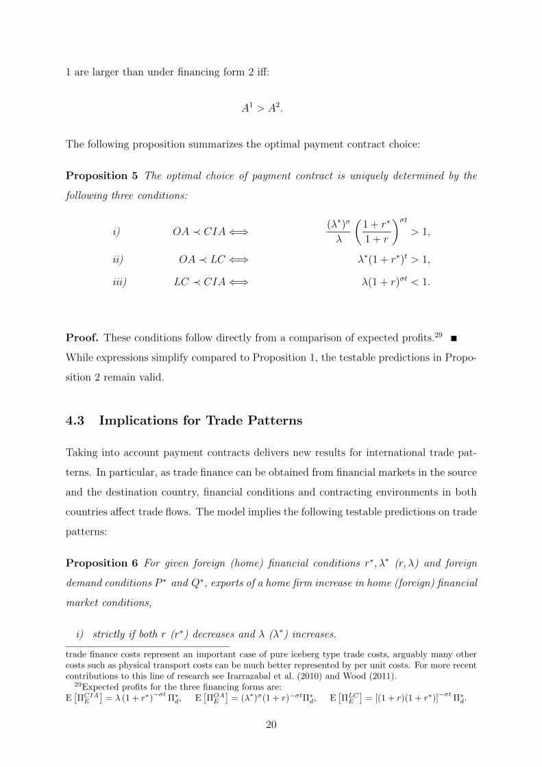
The following proposition summarizes the optimal payment contract choice:

Proposition 5 The optimal choice of payment contract is uniquely determined by the

following three conditions:

i) OA ≺ CIA⇐⇒ (λ∗)σ

λ

(1 + r∗

1 + r

)σt> 1,

ii) OA ≺ LC ⇐⇒ λ∗(1 + r∗)t > 1,

iii) LC ≺ CIA⇐⇒ λ(1 + r)σt < 1.

Proof. These conditions follow directly from a comparison of expected profits.29

While expressions simplify compared to Proposition 1, the testable predictions in Propo-

sition 2 remain valid.

4.3 Implications for Trade Patterns

Taking into account payment contracts delivers new results for international trade pat-

terns. In particular, as trade finance can be obtained from financial markets in the source

and the destination country, financial conditions and contracting environments in both

countries affect trade flows. The model implies the following testable predictions on trade

patterns:

Proposition 6 For given foreign (home) financial conditions r∗, λ∗ (r, λ) and foreign

demand conditions P ∗ and Q∗, exports of a home firm increase in home (foreign) financial

market conditions,

i) strictly if both r (r∗) decreases and λ (λ∗) increases.

trade finance costs represent an important case of pure iceberg type trade costs, arguably many othercosts such as physical transport costs can be much better represented by per unit costs. For more recentcontributions to this line of research see Irarrazabal et al. (2010) and Wood (2011).

29Expected profits for the three financing forms are:E[ΠCIAE

]= λ (1 + r∗)

−σtΠ∗d, E

[ΠOAE

]= (λ∗)σ(1 + r)−σtΠ∗d, E

[ΠLCE

]= [(1 + r)(1 + r∗)]

−σtΠ∗d.

20

ii) weakly if r (r∗) decreases or λ (λ∗) increases.

iii) the more, the larger t.

Proof. See Appendix A.

Exports of a firm decrease in interest rates and increase in enforcement probabilities in

the source and the destination country.30 To bring the model to the data, the following

Corollary is useful.

Corollary 1 For given foreign (home) financial conditions r∗, λ∗ (r, λ) and foreign de-

mand conditions P ∗ and Q∗, the log of exports of a home firm increases in home (foreign)

financial market conditions.

i) strictly if both ln(1 + r) (ln(1 + r∗)) decreases and λ (λ∗) increases

ii) weakly if ln(1 + r) (ln(1 + r∗)) decreases or λ (λ∗) increases

iii) the more in ln(1 + r) (ln(1 + r∗)), the larger t and therefore also, the larger ln t

Proof. See Appendix A.

Corollary 1 implies that the effect of interest rates on trade flows is increasing in t, the

time it takes to transport goods abroad and sell them in the destination country, and

therefore increasing in ln t. This provides the theoretical basis for the distance interactions

employed in the next section.31

4.4 Economic Relevance of Payment Contracts

Is the choice between payment contracts economically relevant? To answer this ques-

tion, I present a numerical example and calculate trade flows in a two country general

equilibrium version of the model.32 Suppose there are three types of countries as de-

scribed in Table 1. Type I has a very efficient financial market and strong enforcement.

Type II has a relatively efficient financial market, but enforcement is weak. Type III has

30It would be straightforward to extend the model to a heterogenous firms framework featuring selectioninto exporting. Then, analog propositions for the extensive margin could be derived.

31Payment contracts also imply testable prediction for observed FOB prices. For details see AppendixD.

32See Appendix C for the formal derivation.

21

a less efficient financial market, but relatively strong enforcement.33 As shown earlier,

Table 1. Country Types

This table reports the values for contract enforcement λ and interest rates 1+r for the numerical examplein Section 4.4. Time to trade t is assumed to be 2 months. Annualized rates for working capital financingare 1.05, 1.07 and 1.14 for the three country types, respectively.

Country Type I II IIIλ 0.99 0.94 0.98

1 + r 1.0082 1.0113 1.0221

these country characteristics determine the optimal payment contract for each exporter-

importer country combination. The optimal payment contracts chosen are reported in

table 2. Suppose firms can choose Open Account, whereas Cash in Advance and Letter

Table 2. Optimal Payment Contracts

This table reports the optimal payment contracts chosen for trade between the three types of countries.Available contracts are Cash in Advance (CIA), Open Account (OA) and Letter of Credit (LC).

from / to I II IIII CIA CIA CIAII LC LC OAIII CIA CIA CIA

of Credit are not available. This case corresponds to exporter finance only. Below, I

report the percentage decrease in traded quantities implied by this restriction of the pay-

ment contract choice. Table 3 therefore quantifies the difference in predicted trade flows

between this model and previous models that abstract from the full choice of payment

contracts available.34 If, for example, an exporter in a country of Type I trading with

an importer in a country of Type II is forced to use OA instead of CIA, this reduces her

exported quantity by 16.1 percent. The results show that the choice between payment

contracts is economically relevant and that its effects are heterogeneous across country

pairs. Some trade, like trade between Type I countries, does not depend very much on

33For this example, t is assumed to be 2 months. Interest rates in the table are adjusted to this shorttime horizon. Annualized rates for working capital financing in this example are 1.05, 1.07 and 1.14 forthe three country types, respectively.

34The calculations are done solving the two country model for every country type combination sep-arately. Exporters both in the home country and the foreign country are assumed to be constrainedto use Open Account only. Reverse trade flows (from abroad to home), which are not reported here,have an impact on price levels and thus on traded quantities of home country exporters. Due to generalequilibrium effects, restricting payment contracts can therefore increase exports by home firms.

22

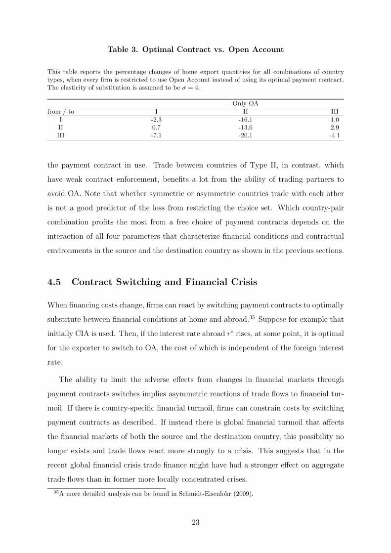
Table 3. Optimal Contract vs. Open Account

This table reports the percentage changes of home export quantities for all combinations of countrytypes, when every firm is restricted to use Open Account instead of using its optimal payment contract.The elasticity of substitution is assumed to be σ = 4.

Only OAfrom / to I II III

I -2.3 -16.1 1.0II 0.7 -13.6 2.9III -7.1 -20.1 -4.1

the payment contract in use. Trade between countries of Type II, in contrast, which

have weak contract enforcement, benefits a lot from the ability of trading partners to

avoid OA. Note that whether symmetric or asymmetric countries trade with each other

is not a good predictor of the loss from restricting the choice set. Which country-pair

combination profits the most from a free choice of payment contracts depends on the

interaction of all four parameters that characterize financial conditions and contractual

environments in the source and the destination country as shown in the previous sections.

4.5 Contract Switching and Financial Crisis

When financing costs change, firms can react by switching payment contracts to optimally

substitute between financial conditions at home and abroad.35 Suppose for example that

initially CIA is used. Then, if the interest rate abroad r∗ rises, at some point, it is optimal

for the exporter to switch to OA, the cost of which is independent of the foreign interest

rate.

The ability to limit the adverse effects from changes in financial markets through

payment contracts switches implies asymmetric reactions of trade flows to financial tur-

moil. If there is country-specific financial turmoil, firms can constrain costs by switching

payment contracts as described. If instead there is global financial turmoil that affects

the financial markets of both the source and the destination country, this possibility no

longer exists and trade flows react more strongly to a crisis. This suggests that in the

recent global financial crisis trade finance might have had a stronger effect on aggregate

trade flows than in former more locally concentrated crises.

35A more detailed analysis can be found in Schmidt-Eisenlohr (2009).

23

5 Empirical Tests

The model predicts that financing costs affect trade flows. An increase in interest rates in

the source and the destination country makes trade finance more costly, implying higher

export prices and lower export quantities and revenues. Proposition 6 states that the

size of this effect should be proportional to the time needed for trade. I use a panel of

bilateral trade data to test these predictions.

The analysis proceeds in four steps. First, the baseline regression is presented, pro-

viding evidence for a negative relationship between financing costs and trade flows. I

find that the size of the effect of financing costs on trade flows is increasing in the geo-

graphical distance between trading partners. Second, based on the results of the baseline

regression, I study comparative statics and show that the relationship is economically

relevant. Next, I check the robustness of my results. The introduction of interaction

terms between geographical distance and measures of contract enforcement (rule of law)

and economic development (log of GDP per capita) to the regression does not change

the main findings. Results also hold when I introduce exporter × year and importer ×

year fixed effects and estimate a fixed effects model. Replacing the net interest margin

by private capital over GDP as the variable capturing financial conditions delivers very

similar results. Finally, I address the question of causality.

5.1 Data

I use data on bilateral trade flows for the years 1980 to 2004 from the CEPII trade and

production database. Data on geographical distance and other bilateral indicators is

from the CEPII gravity dataset collected by Head et al. (2010). The financial market

efficiency (net interest margin) and financial market development measures (private credit

over GDP) are taken from Beck et al. (2009). The net interest margin is the ratio between

the accounting value of the net interest revenues of banks and their total earning assets.

It measures the average ex-post markup of the lending activities of banks in a country and

therefore represents a measure of financial sector efficiency. This measure differs from ex-

ante spreads as it also captures losses on non-performing loans. The alternative measure,

private credit over GDP, is a much broader indicator of general financial development.

24

While the latter seems more appropriate for studying financial constraints, the former

seems better suited for addressing the question of trade finance and its effects on variable

costs studied here. Data on GDP per capita and population are taken from the Penn

World Tables (Heston et al. (2009)). The measure for contract enforcement is extracted

from the World Bank Worldwide Governance Indicators. The final sample contains 150

exporting countries over the period 1980-2004. When including the net interest rate

margin the number of countries reduces to 144 and the period to 1987-2004. With

contract enforcement the years covered are 1998, 2000, and 2002-2004.

5.2 Estimation and Results

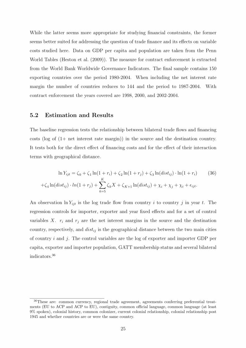
The baseline regression tests the relationship between bilateral trade flows and financing

costs (log of (1+ net interest rate margin)) in the source and the destination country.

It tests both for the direct effect of financing costs and for the effect of their interaction

terms with geographical distance.

lnYijt = ζ0 + ζ1 ln(1 + ri) + ζ2 ln(1 + rj) + ζ3 ln(distij) · ln(1 + ri) (36)

+ζ4 ln(distij) · ln(1 + rj) +K∑k=5

ζkX + ζK+1 ln(distij) + χi + χj + χt + εijt.

An observation lnYijt is the log trade flow from country i to country j in year t. The

regression controls for importer, exporter and year fixed effects and for a set of control

variables X. ri and rj are the net interest margins in the source and the destination

country, respectively, and distij is the geographical distance between the two main cities

of country i and j. The control variables are the log of exporter and importer GDP per

capita, exporter and importer population, GATT membership status and several bilateral

indicators.36

36These are: common currency, regional trade agreement, agreements conferring preferential treat-ments (EU to ACP and ACP to EU), contiguity, common official language, common language (at least9% spoken), colonial history, common colonizer, current colonial relationship, colonial relationship post1945 and whether countries are or were the same country.

25

Table

4.

Fin

anci

ng

Cost

s,D

ista

nce

and

Exp

ort

Volu

mes

Th

ista

ble

anal

yze

sth

eeff

ects

offi

nan

cin

gco

sts

inth

eex

port

ing

an

dim

port

ing

cou

ntr

yan

dth

eir

inte

ract

ion

sw

ith

dis

tance

on

exp

ort

volu

mes

.T

he

dep

enden

tva

riab

leis

the

log

ofex

por

tsfr

omco

untr

yi

toco

untr

yj

inye

ar

t,1987-2

004.

Fin

an

cin

gco

sts

are

mea

sure

dby

the

net

inte

rest

marg

in.

Tim

eto

trad

eis

pro

xie

dby

the

geog

rap

hic

ald

ista

nce

bet

wee

nth

em

ain

citi

esof

two

cou

ntr

ies.

Contr

act

enfo

rcem

ent

isp

roxie

dby

Ru

leof

Law

.R

egre

ssio

ns

inco

lum

ns

1an

d2

contr

ol

for

the

log

ofG

DP

per

cap

ita,

pop

ula

tion

and

GA

TT

stat

us

for

exp

ort

eran

dim

port

er,

resp

ecti

vely

.R

egre

ssio

ns

incl

ud

ea

con

stant

an

dco

lum

ns

1th

rou

gh

4co

ntr

olfo

ra

set

ofb

ilat

eral

contr

ols

asd

iscu

ssed

inth

ete

xt.

Colu

mn

2als

oco

ntr

ols

for

contr

act

enfo

rcem

ent

inb

oth

cou

ntr

ies.

Err

ors

are

clust

ered

by

exp

orte

r-im

por

ter

pai

rs.

Sta

nd

ard

erro

rsar

ein

par

enth

esis

.S

ign

ifica

nce

leve

ls:∗

:10%∗∗

:5%∗∗∗

:1%

.

Dep

end

ent

vari

able

lnb

ilate

ral

exp

ort

sS

pec

ifica

tion

(1)

(2)

(3)

(4)

(5)

(6)

Ln

exp

int

39.1

05***

12.0

88***

(2.9

4)

(3.9

9)

Ln

imp

int

47.1

59***

21.6

49***

(3.0

6)

(3.8

6)

Ln

exp

int

xln

dis

t-4

.783

***

-1.6

70***

-5.2

41***

-2.1

47***

-0.4

69**

-0.0

82

(0.3

5)

(0.4

6)

(0.3

7)

(0.4

9)

(0.2

1)

(0.3

7)

Ln

imp

int

xln

dis

t-5

.752

***

-2.6

54***

-6.2

75***

-2.9

55***

-1.4

32***

-2.3

41***

(0.3

6)

(0.4

5)

(0.3

8)

(0.4

8)

(0.2

1)

(0.3

7)

Exp

law

xln

dis

t0.2

20***

0.2

15***

-0.0

49

(0.0

3)

(0.0

3)

(0.0

3)

Imp

law

xln

dis

t0.1

04***

0.0

91***

0.0

14

(0.0

3)

(0.0

3)

(0.0

3)

Ln

GD

PE

xln

dis

t-0

.058**

-0.0

57**

0.0

07

(0.0

3)

(0.0

3)

(0.0

6)

Ln

GD

PI

xln

dis

t0.1

64***

0.1

73***

0.1

19**

(0.0

3)

(0.0

3)

(0.0

6)

Ln

dis

t-0

.883

***

-2.2

00***

-0.8

44***

-2.2

51***

(0.0

3)

(0.2

9)

(0.0

3)

(0.3

0)

R-s

qu

ared

0.79

80.7

94

0.8

07

0.8

01

0.1

82

0.1

45

N14

2761

78742

142761

78742

142761

78742

#ex

por

ter-

imp

orte

rcl

ust

ers

1826

017924

18260

17924

18260

17924

#ex

por

ters

144

144

144

144

144

144

Cou

ntr

yco

ntr

ols

yy

--

--

Cou

ntr

yp

air

contr

ols

yy

yy

yy

Imp

orte

r,ex

por

ter,

year

FE

yy

nn

nn

Imp×

year

,ex

p×

year

FE

nn

yy

yy

Cou

ntr

yp

air

FE

nn

nn

yy

26

Distance effect The regression reported in Column 1 of Table 4 provides evidence that

financial conditions are correlated with trade flows. Countries with higher net interest

rate margins trade less with each other. The size of this effect is increasing in the

geographical distance between trading partners. This can be seen by noting that, in

line with Corollary 1, both coefficients on the distance interaction ζ3 and ζ4 are highly

significant and negative. The preferred specification is presented in column 3, where

exporter × year and importer × year fixed effects are included. In this specification ζ3

and ζ4 are larger and also highly significant.

Economic relevance The marginal effects of financing costs evaluated at the mean

log bilateral distance (8.6) for the regressions in columns 1 and 2 are reported in Table

5. They imply that a one percent higher financing cost in a country is associated with

2.0 percent lower exports and 2.3 percent lower imports by that country. To evaluate the

Table 5. Marginal effects of change in financing costs

This table reports the marginal effects for the regression results in Table 4. The values represent thepercentage changes of exports and imports, respectively, resulting from a one percent increase in financingcosts (1+net interest margin) evaluated at the sample mean bilateral distance (8.6). Columns (1) and(2) correspond to columns (1) and (2) in Table 4. Standard errors are in parenthesis. Significance levels:∗ : 10% ∗∗ : 5% ∗ ∗ ∗ : 1%.

Effects from 1 % increase in financing costs

Specification (1) (2)Exports -2.002*** -2.270***

(0.31) (0.39)Imports -2.280*** -1.174***

(0.30) (0.38)Mean ln dist 8.595 8.599N 142761 78742

economic relevance of the distance interaction, consider the following comparative statics.

Compare trade between Spain and Egypt (25 percentile by distance, 3355 km) with trade

between Spain and South Korea (75 percentile by distance, 10013km). Suppose the net

interest margin in Spain was one percent higher. Then we should expect Spain to have a

5.2 percent larger drop of its exports and a 6.3 percent larger drop of its imports when

trading with South Korea instead of Egypt due to the larger geographical distance. Table

6 reports comparative statics for all specifications from Table 4.

27

Table 6. Comparative statics for change in financing costs

This table reports comparative statics for the regression results in Table 4. I compare trade between acountry pair at the 25 distance percentile (e.g. Spain - Egypt, 3355km) with trade between a country pairat the 75 distance percentile (e.g. Spain - South Korea, 10013km). Values report the reaction of tradeto a one percent increase in financing costs (1+net interest margin). Standard errors are in parenthesis.Significance levels: ∗ : 10% ∗∗ : 5% ∗ ∗ ∗ : 1%.

Effects from 1 % increase in financing costs

Specification (1) (2) (3) (4) (5) (6)Exports

25 distance 0.278 -1.468*** - - - -percentile (0.33) (0.44) - - - -75 distance -4.951*** -3.293*** - - - -percentile (0.40) (0.48) - - - -Difference -5.230*** -1.826*** -5.730*** -2.347*** -0.512** -0.089

(0.38) (0.51) (0.40) (0.54) (0.23) (0.40)Imports

25 distance 0.463 0.102 - - - -percentile (0.33) (0.42) - - - -75 distance -5.827*** -2.800*** - - - -percentile (0.39) (0.48) - - - -Difference -6.289*** -2.902*** -6.861*** -3.231*** -1.566*** -2.560***

(0.39) (0.49) (0.42) (0.53) (0.23) (0.41)N 142761 78742 142761 78742 142761 78742

Robustness One concern is potential omitted variable bias. If there are variables that

are correlated with the net interest rate margin and bilateral trade flows that are not

included in the regression, the estimate of the distance interaction can be biased. To

address this issue, Columns 2, 4 and 6 introduce two additional interaction terms. A

measure of contract enforcement (rule of law) and its interaction with distance are added

to the regression to control for institutional factors. An interaction between the log of

GDP per capita and distance is added to control for effects from the general economic

development of countries. Comparing column 2 to column 1, the introduction of these

additional regressors reduces the point estimates for ζ3 and ζ4 to about a half of their

previous values. They remain highly significant and economically relevant.

Columns 5 and 6 estimate a fixed effects model, where effects are identified from

within country pair variation over time.37 ζ3 and ζ4 become smaller but remain highly

significant with the exception of ζ4 in column 6.38

Another concern might be the measure for financial conditions employed in the re-

37This resolves the time-invariant part of the omitted variable bias discussed in Anderson and vanWincoop (2003). An alternative would be to follow Baier and Bergstrand (2009) and explicitly introduceexogenous multilateral-resistance terms.

38This might be due to collinearity, that is the high correlation between the net interest margin andper capita GDP (-.47) and contract enforcement (-.54), respectively.

28

gressions so far. The choice of the net interest margin is motivated by the theoretical

part of the paper, which focuses on financing costs of international trade. An alternative

is to use private credit over GDP as a general measure for financial development, first

introduced to the literature by Beck (2002). This is the standard measure used as a

proxy for financial conditions, in particular, in papers that study the role of financial

constraints. As a robustness check, I rerun the regressions shown in Table 4 Columns

1 to 4, using private credit over GDP instead of the net interest margin. The results

are reported in Table 7. They support the findings from the previous regressions. Note

that financial development increases in the ratio of private credit over GDP. That is, the

higher the ratio, the better are financial conditions. Therefore, all coefficients on the

financial measure have exactly the opposite sign from the regressions in Table 4. Can we

interpret the relationship identified by the interaction terms between distance and the

measures of financial conditions as causal? The main concern in this context is reverse

causality. If a country conducts a lot of international trade, this increases its demand for

financial services. A larger demand in turn can lead to efficiency gains in the provision

of finance, reducing the net interest rate margin.39 As discussed earlier, the distance

interaction identifies effects proportional to the geographical distance between trading

partners. Therefore, the relevant reverse causality to be considered is the following. Sup-

pose there is an increase in the demand from a destination country. This increases the

demand for trade finance in the source country proportional to the geographical distance

from this trading partner. Reverse causality is a problem if international trade working

capital financing is sufficiently large to have a first-order effect on the overall demand for

finance in a country. While lending related to international trade finance is certainly an

important activity in many countries, it can be argued that in most cases it represents

a relatively small share of overall finance. A first-order effect from trade finance on the

borrowing rate of firms therefore seems unlikely. This suggests that there is a causal

effect of financing costs on trade, proportional to distance.

39Do and Levchenko (2007) and Braun and Raddatz (2008) find evidence for reverse causality fromtrade flows and trade openness, respectively, to financial development.

29

Table 7. Financial Development, Distance and Export Volumes

This table analyzes the relationship between financial development in the source and the destinationcountry and export volumes. The regressions test for a direct effect of financial development and foran effect of its interaction with distance. The dependent variable is the log of exports from country ito country j in year t, 1980-2004. Financial development is proxied by private credit over GDP. Timeto trade is proxied by the geographical distance between the main cities of two countries. Contractenforcement is proxied by rule of law. Regressions in columns 1 and 2 control for the log of GDP percapita, population and GATT status for exporter and importer, respectively. Regressions include aconstant and columns 1 through 4 control for a set of bilateral controls as discussed in the text. Column2 also controls for contract enforcement in both countries. Errors are clustered by exporter-importerpairs. Standard errors are in parenthesis. ∗, ∗∗ and ∗ ∗ ∗ denote significance at the 10%, 5% and 1%level.

Dependent variable ln bilateral exportsSpecification (1) (2) (3) (4)Exp fin devt -4.465*** -3.211***

(0.29) (0.37)Imp fin devt -5.327*** -2.260***

(0.30) (0.41)Exp fin devt x ln dist 0.523*** 0.360*** 0.552*** 0.371***

(0.03) (0.04) (0.03) (0.04)Imp fin devt x ln dist 0.606*** 0.256*** 0.618*** 0.263***

(0.03) (0.05) (0.04) (0.05)Exp law x ln dist 0.143*** 0.156***

(0.03) (0.03)Imp law x ln dist 0.022 0.009

(0.03) (0.03)Ln GDPE x ln dist -0.095*** -0.104***

(0.03) (0.03)Ln GDPI x ln dist 0.161*** 0.172***

(0.03) (0.03)ln dist -1.981*** -2.365*** -2.024*** -2.390***

(0.03) (0.27) (0.03) (0.28)R-squared 0.772 0.786 0.788 0.792N 228045 82812 228045 82812# exporter-importer clusters 19253 18262 19253 18262# exporters 150 150 150 150Country controls y y - -Country pair controls y y y yImporter, exporter, year FE y y n nImp × year, exp × year FE n n y y

30

6 Conclusions

Firms in international trade utilize different payment contract to optimally trade off dif-

ferences in financing costs and contractual environments between source and destination

countries. Financial conditions have large effects on bilateral trade flows, with costs in

the destination country being more important than those in the source country. This is

in stark contrast to most of the literature on finance and trade which almost exclusively

focused on the role of conditions in the source country. While standard trade theory

abstracts from the explicit modeling of importers, the theory and empirical results in this

paper show that it can be important to consider the actual trade relationships between

firms in two countries; in particular, to consider an exporter and an importer as well as

potentially other actors such as banks. In this, my paper is related to a growing literature

departing from the view of exporters selling directly to customers in the foreign market.40

The model could be extended allowing for heterogeneity both in the firm and in the

product dimension. Product differences could imply different degrees of enforceability

in court or different time horizons of trade relationships. Firm differences in size could

affect the relative negotiation power between the exporter and the importer, the ability

to enforce contracts in court, to punish deviations from a trigger strategy and to switch

contracts in the face of fixed costs. In an extension, currencies could be introduced to

study the interaction of the payment contract decision with exchange rate risk.

While the aggregate regressions in this paper constitute a first step, more empirical

work is desirable. A dataset containing information on payment contracts, for example,

could be used to test the predictions from Sections 2 and 3.

Finally, following Greif (1993), historical trade patterns could be studied in light of the

trade-off between financial market characteristics and contracting environments between

source and destination country derived in the model. Improvements in institutions over

time should be related to the types of payment contracts utilized.

40See for example Bernard et al. (2010), Antras and Costinot (forthcoming) and Ahn et al. (forthcom-ing).

31

A Proofs

Proof of Proposition 6 Expected quantities are E [qx] = Aq∗d = ασβ1−σq∗d, and ex-

pected revenues are E [Rx] = pxE [qx] = βαAR∗d = ασ−1β2−σR∗d. As q∗d and R∗d are held

constant, it remains to be shown that A and βαA behave has stated in the Proposition.

For the three different financing forms we have:

ACIA = λ(1 + r∗)−σtβCIA

αCIAACIA = λ(1 + r∗)(1−σ)t

AOA = (λ∗)σ(1 + r)−σtβOA

αOAAOA = (λ∗)σ−1(1 + r)(1−σ)t

ALC = [(1 + r)(1 + r∗)]−σtβLC

αLCALC = [(1 + r)(1 + r∗)](1−σ)t.

First, note that whenever a firm changes its payment contract, this implies that its

expected profits, quantities and profits under the new contract are at least as large as

under the old contract. Therefore, to prove the Proposition, it is sufficient to show that

the statements on export revenues and quantities hold when there is no contract change.

Hence, noting that σ > 1, i) and ii) follow directly from taking derivatives with respect

to r, r∗, λ and λ∗, respectively. Taking cross-derivatives with respect to t and r, r∗, λ

and λ∗, respectively, proves iii).

Proof of Corollary 1 The log of expected quantities is ln E [qx] = lnA+ ln q∗d and the

log of expected revenues is ln E [Rx] = ln(βαA)

+ lnR∗d. As q∗d and R∗d are held constant,

it remains to be shown that lnA and ln(βαA)

behave as stated in the Corollary. For the

three different financing forms we have:

lnACIA = lnλ− σt ln(1 + r∗) ln

(βCIA

αCIAACIA

)= lnλ− (σ − 1)t ln(1 + r∗)

lnAOA = σ lnλ∗ − σt ln(1 + r) ln

(βOA

αOAAOA

)= (σ − 1) lnλ∗ − (σ − 1) ln t(1 + r)

lnALC = −σt[ln(1 + r) + ln(1 + r∗)] ln

(βLC

αLCALC

)= −(σ − 1)t[ln(1 + r) + ln(1 + r∗)].

The statement in the Proof of Proposition 6 on contract switching remains valid. Again,

i) and ii) follow from taking derivatives with respect to r, r∗, λ and λ∗, respectively. iii)

follows from taking cross-derivatives with respect to t and r, r∗, λ and λ∗, respectively.

32

B Wealth constraints

This section shows that a model with a limited value of contract constraint represents

a special case of a model with wealth constraints, where the wealth of the importer is

set to zero. Let Wi denote the level of wealth of a firm, which it can use to pay for any

transactions additional to any cash flow created arising from its economic activities.41

Assume for now that exporters have sufficient wealth to finance production, i.e. WE >

K.42 Assume that (under CIA and LC) the importer can borrow against her expected

future cash-flow from the trade transaction. Then, under CIA, the new expected profit

maximization problem is:

maxC

E[ΠCIAE

]= CCIA − λK,

s.t. CCIA ≤ WI +λR

1 + r∗, (wealth constraint)

and E[ΠCIAI

]= λR− (1 + r∗)CCIA ≥ 0. (participation constraint importer)

The wealth constraint never binds and results do not change. Under OA the new expected

profit maximization problem is:

maxC

E[ΠOAE

]=

1

1 + r(λ∗COA −K(1 + r)),

s.t. COA ≤ R +WI , (wealth constraint)

and E[ΠOAI

]=

1

1 + r∗(R− λ∗COA) ≥ 0, (participation constraint importer)

41The model could be extended to allow firms to borrow using their wealth as collateral. Then, theamount of credit accessible would be increasing in the level of wealth and affected by institutional factorssuch as enforcement and bankruptcy procedures.

42This assumption is to exclude some cases, which seem to be less interesting for the current analysis.Note though, that payment contracts can indeed be a way to circumvent financial constraints for ex-porters. This point is related to the use of foreign FDI to finance production in countries with strongerfinancing constraints. In a Melitz (2003) type heterogeneous firms setup, payment contracts may be alsoused to shift the financing of sunk fixed costs of exporting towards the importer’s financial market.

33

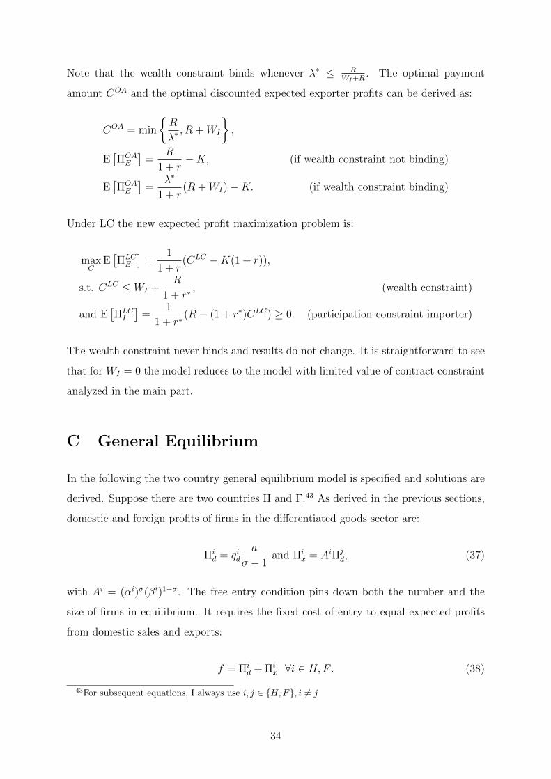
Note that the wealth constraint binds whenever λ∗ ≤ RWI+R

. The optimal payment

amount COA and the optimal discounted expected exporter profits can be derived as:

COA = min

R

λ∗, R +WI

,

E[ΠOAE

]=

R

1 + r−K, (if wealth constraint not binding)

E[ΠOAE

]=

λ∗

1 + r(R +WI)−K. (if wealth constraint binding)

Under LC the new expected profit maximization problem is:

maxC

E[ΠLCE

]=

1

1 + r(CLC −K(1 + r)),

s.t. CLC ≤ WI +R

1 + r∗, (wealth constraint)

and E[ΠLCI

]=

1

1 + r∗(R− (1 + r∗)CLC) ≥ 0. (participation constraint importer)

The wealth constraint never binds and results do not change. It is straightforward to see

that for WI = 0 the model reduces to the model with limited value of contract constraint

analyzed in the main part.

C General Equilibrium

In the following the two country general equilibrium model is specified and solutions are

derived. Suppose there are two countries H and F.43 As derived in the previous sections,

domestic and foreign profits of firms in the differentiated goods sector are:

Πid = qid

a

σ − 1and Πi

x = AiΠjd, (37)

with Ai = (αi)σ(βi)1−σ. The free entry condition pins down both the number and the

size of firms in equilibrium. It requires the fixed cost of entry to equal expected profits

from domestic sales and exports:

f = Πid + Πi

x ∀i ∈ H,F . (38)

43For subsequent equations, I always use i, j ∈ H,F, i 6= j

34

The two free entry conditions can be solved for domestic and export quantities:44

qid =σ − 1

af

1− Ai

1− AiAj, qix = Aiqjd =

σ − 1

afAi(1− Aj)1− AiAj

. (40)

Total expected quantities are constant:

qi =σ − 1

af. (41)

Labor market clearing The number of firms in both countries is determined by the

labor market clearing condition.45 Given the CD preferences, a constant fraction of labor

is employed by the differentiated sector:

LiQ = µLi. (42)

Labor in the differentiated sector is used for entry and production:

LiQ = LiE + LiP = ni(f + aq). (43)

The number of firms can be derived as:

n =µLi

f + aq=µLi

σf. (44)

D FOB Prices

Given per unit cost a, different payment contracts imply different FOB prices. To see

this, note that from before the agreed on payment amounts C differ by payment contract,

44Plugging in the values derived for profits from before delivers:

f =a

σ − 1

[qid +Aiqjd

]. (39)

45For tractability, I assume that the positive expected profits of importers under Open Account donot enter the demand for differentiated good. It would be interesting to analyze these ’informal’ profitsexplicitly in the general equilibrium. This could be relevant for countries with very low enforcementrates.

35

i.e.:

CCIA =λ

1 + r∗RCIA, COA = ROA, CLC =

RLC

1 + r∗. (45)

This implies the following testable prediction:

Proposition 7 Suppose RCIA = ROA = RLC, λ < 1 and r∗ > 0. Then,

COA > CLC > CCIA.

Proof. Follows directly from Equations 45.

R is the amount of sales revenues in the importing country when trade takes place:

R =

(β

α

)1−σ

r∗d. (46)

The following payment amounts corresponding to FOB prices can be derived:

CCIA = λ(1 + r∗)−σr∗d, COA = (λ∗)σ−1(1 + r)1−σr∗d, CLC = (1 + r)1−σ(1 + r∗)−σr∗d.(47)

From this it can be seen that the amounts specified to be paid for the traded goods vary

with financial market parameters in a systematic way. Depending on the payment form

used, financial parameters affect FOB prices differentially. In an empirical analysis of

FOB price data, it might thus be relevant to control for differences in payment contracts.

Estimates regarding FOB prices and financial indicators might otherwise be biased.

36

References

Ahn, JaeBin, “A Theory of Domestic and International Trade Finance,” 2010. Columbia

University, mimeo.

, Amit K. Khandelwal, and Shang-Jin Wei, “The role of intermediaries in facili-

tating trade,” Journal of International Economics, forthcoming.

Alchian, Armen and William Allen, University Economics, Belmont, California:

Wadsworth, 1964.

Alessandria, George, Joseph P. Kaboski, and Virgiliu Midrigan, “The Great

Trade Collapse of 2008-09: An Inventory Adjustment?,” NBER Working Papers 16059,

National Bureau of Economic Research, Inc June 2010.

Amiti, Mary and David E. Weinstein, “Exports and Financial Shocks,” mimeo,

Federal Reserve Bank of New York and Columbia University October 2009.

Anderson, James E. and Eric van Wincoop, “Gravity with Gravitas: A Solution

to the Border Puzzle,” American Economic Review, March 2003, 93 (1), 170–192.

Antras, Pol and Arnaud Costinot, “Intermediated Trade,” Quarterly Journal of

Economics, forthcoming.

, Mihir A. Desai, and C. Fritz Foley, “Multinational Firms, FDI Flows, and

Imperfect Capital Markets*,” Quarterly Journal of Economics, 2009, 124 (3), 1171–

1219.

Baier, Scott L. and Jeffrey H. Bergstrand, “Bonus vetus OLS: A simple method

for approximating international trade-cost effects using the gravity equation,” Journal

of International Economics, February 2009, 77 (1), 77–85.

Beck, Thorsten, “Financial Development and International Trade: Is there a Link?,”

Journal of International Economics, June 2002, 57 (1), 107–131.

, “Financial Dependence and International Trade,” Review of International Economics,

May 2003, 11 (2), 296–316.

37

, Asli Demirguc-Kunt, and Ross Levine, “Financial institutions and markets

across countries and over time - data and analysis,” Policy Research Working Paper

Series 4943, The World Bank May 2009.

Behrens, Kristian, Gregory Corcos, and Giordano Mion, “Trade Crisis? What

Trade Crisis?,” CEPR Discussion Papers 7956, C.E.P.R. Discussion Papers August

2010.

Berman, Nicolas and Jerome Hericourt, “Financial factors and the margins of

trade: Evidence from cross-country firm-level data,” Journal of Development Eco-

nomics, 2010, 93 (2), 206 – 217.

and Philippe Martin, “The Vulnerability of Sub-Saharan Africa to the Financial

Crisis: The Case of Trade,” May 2009. mimeo.

Bernard, Andrew B., J. Bradford Jensen, Stephen J. Redding, and Peter K.

Schott, “Wholesalers and Retailers in US Trade,” American Economic Review Papers

& Proceedings, May 2010, 100 (2), 408–13.

Biais, Bruno and Christian Gollier, “Trade Credit and Credit Rationing,” Review

of Financial Studies, 1997, 10 (4), 903–37.

Braun, Matias and Claudio Raddatz, “The Politics of Financial Development: Ev-

idence from Trade Liberalization,” Journal of Finance, June 2008, 63 (3), 1469–1508.

Bricongne, Jean-Charles, Lionel Fontagne, Guillaume Gaulier, Daria Taglioni,

and Vincent Vicard, “Firms and the global crisis: French exports in the turmoil,”

Working Paper Series 1245, European Central Bank 2010.

Burkart, Mike and Tore Ellingsen, “In-Kind Finance: A Theory of Trade Credit,”

American Economic Review, June 2004, 94 (3), 569–590.

Chaney, Thomas, “Liquidity Constrained Exporters,” Technical Report, University of

Chicago July 2005.

Chor, Davin and Kalina Manova, “Off the Cliff and Back? Credit Conditions and

International Trade during the Global Financial Crisis,” NBER Working Papers 16174,

National Bureau of Economic Research, Inc July 2010.

38

Cunat, Vicente, “Trade Credit: Suppliers as Debt Collectors and Insurance Providers,”

The Review of Financial Studies, 2007, 20 (2), 491–527.

Djankov, Simeon, Caroline Freund, and Cong S Pham, “Trading on Time,” The

Review of Economics and Statistics, May 2010, 92 (1), 166–173.

Do, Quy-Toan and Andrei A. Levchenko, “Comparative advantage, demand for ex-

ternal finance, and financial development,” Journal of Financial Economics, December

2007, 86 (3), 796–834.

Eaton, Jonathan and Samuel Kortum, “Technology, Geography, and Trade,” Econo-

metrica, September 2002, 70 (5), 1741–1779.

, , Brent Neiman, and John Romalis, “Trade and the Global Recession,” 2009.

Penn State and University of Chicago, mimeo.

Ellingsen, Tore and Jonas Vlachos, “Trade finance in a liquidity crisis,” Policy

Research Working Paper Series 5136, The World Bank November 2009.

Giannetti, Mariassunta, Mike Burkart, and Tore Ellingsen, “What You Sell Is

What You Lend? Explaining Trade Credit Contracts,” Review of Financial Studies,

forthcoming.

Greenaway, David, Alessandra Guariglia, and Richard Kneller, “Financial Fac-

tors and Exporting Decisions,” Journal of International Economics, November 2007,

73 (2), 377–395.

Greif, Avner, “Contract Enforceability and Economic Institutions in Early Trade: the

Maghribi Traders’ Coalition,” American Economic Review, June 1993, 83 (3), 525–48.

Head, Keith, Thierry Mayer, and John Ries, “The erosion of colonial trade linkages

after independence,” Journal of International Economics, May 2010, 81 (1), 1–14.

Helpman, Elhanan, “Trade, FDI, and the Organization of Firms,” Journal of Economic

Literature, September 2006, 44 (3), 589–630.

and Paul Krugman, Market Structure and Foreign Trade: Increasing Returns,

Imperfect Competition, and the International Economy, The MIT Press, 1985.

39

Heston, Alan, Robert Summers, and Bettina Aten, “Penn World Table Version

6.3,” Technical Report, Center for International Comparisons of Production, Income

and Prices at the University of Pennsylvania August 2009.

Hummels, David, “Time as a Trade Barrier,” GTAP Working Papers 1152, Center

for Global Trade Analysis, Department of Agricultural Economics, Purdue University

2001.

, “Transportation Costs and International Trade in the Second Era of Globalization,”

Journal of Economic Perspectives, Summer 2007, 21 (3), 131–154.

and Alexandre Skiba, “Shipping the Good Apples Out? An Empirical Confirmation

of the Alchian-Allen Conjecture,” Journal of Political Economy, December 2004, 112

(6), 1384–1402.

Humphrey, John, “Are Exporters in Africa Facing Reduced Availability of Trade Fi-

nance,” March 2009. Institute of Development Studies, mimeo.

Iacovone, Leonardo and Veronika Zavacka, “Banking Crises And Exports,” Policy

Research Working Paper Series, The World Bank 2009.

IMF, “Sustaining the Recovery,” World Economic Outlook, International Monetary Fund

October 2009.

Irarrazabal, Alfonso, Andreas Moxnes, and Luca David Opromolla, “The Tip of

the Iceberg: Modeling Trade Costs and Implications for Intra-Industry Reallocation,”

CEPR Discussion Papers 7685 February 2010.

Jacks, David S., Christopher M. Meissner, and Dennis Novy, “Trade Costs, 1870-

2000,” American Economic Review Papers & Proceedings, May 2008, 98 (2), 529–34.

Kletzer, Kenneth and Pranab Bardhan, “Credit Markets and Patterns of Interna-

tional Trade,” Journal of Development Economics, October 1987, 27 (1-2), 57–70.

Korinek, Jane, Jean Le Cocguic, and Patricia Sourdin, “The Availability and

Cost of Short-Term Trade Finance and its Impact on Trade,” OECD Trade Policy

Working Papers 98, OECD 2010.

40

Levchenko, Andrei A., “Institutional Quality and International Trade,” Review of

Economic Studies, July 2007, 74 (3), 791–819.

, Logan Lewis, and Linda L. Tesar, “The Collapse of International Trade During

the 2008-2009 Crisis: In Search of the Smoking Gun,” Discussion Papers, University

of Michigan October 2009.

Manova, Kalina, “Credit constraints, equity market liberalizations and international

trade,” Journal of International Economics, 2008, 76 (1), 33–47.

, “Credit Constraints, Heterogeneous Firms, and International Trade,” NBER Working

Papers 14531, National Bureau of Economic Research December 2008.

Matsuyama, Kiminori, “Credit Market Imperfections and Patterns of International

Trade and Capital Flows,” Journal of the European Economic Association, April/May

2005, 3 (2-3), 714–723.

Melitz, Marc J., “The Impact of Trade on Intra-Industry Reallocations and Aggregate

Industry Productivity,” Econometrica, November 2003, 71 (6), 1695–1725.

Menichini, Anna Maria, “Inter-firm trade finance in times of crisis,” Policy Research

Working Paper Series 5112, The World Bank November 2009.

Muuls, Mirabelle, “Exporters and credit constraints. A firm-level approach,” Research

series 200809-22, National Bank of Belgium September 2008.

Nunn, Nathan, “Relationship-Specificity, Incomplete Contracts, and the Pattern of

Trade,” The Quarterly Journal of Economics, May 2007, 122 (2), 569–600.

Olsen, Morten, “Banks in International Trade: Incomplete International Contract En-

forcement and Reputation,” 2010. Harvard University, mimeo.

Paravisini, Daniel, Veronica Rappoport, Philipp Schnabl, and Daniel Wolfen-

zon, “Dissecting the Effect of Credit Supply on Trade: Evidence from Matched Credit-

Export Data,” 2010. Columbia University, mimeo.

Petersen, Mitchell A and Raghuram G Rajan, “Trade Credit: Theories and Evi-

dence,” Review of Financial Studies, 1997, 10 (3), 661–91.

41

Ronci, Marcio Valerio, “Trade Finance and Trade Flows: Panel Data Evidence from

10 Crises,” IMF Working Papers, International Monetary Fund 2004.

Samuelson, Paul A., “The Transfer Problem and Transport Costs, II: Analysis of

Effects of Trade Impediments,” The Economic Journal, June 1954, 64 (254), 264–289.

Schmidt-Eisenlohr, Tim, “Towards a Theory of Trade Finance,” EUI Working Paper

2009/43, European University Institute December 2009.

van der Veer, Koen, “The Private Credit Insurance Effect on Trade,” DNB Working

Papers 264, De Nederlandsche Bank October 2010.

Wagner Ricci, Cecilia and Gail Morrison, “International Working Capital Practices

of the Fortune 200.,” Financial Practice & Education, 1996, 6 (2), 7–20.

Wilner, Benjamin S., “The Exploitation of Relationships in Financial Distress: The

Case of Trade Credit,” Journal of Finance, February 2000, 55 (1), 153–178.

Wood, Adrian, “A more general Heckscher-Ohlin model,” QEH Working Papers 185,

Queen Elizabeth House, University of Oxford 2011.

Yi, Kei-Mu, Rudolfs Bems, and Robert Christopher Johnson, “Demand

Spillovers and the Collapse of Trade in the Global Recession,” IMF Working Papers

10/142, International Monetary Fund 2010.

42