Towards an Evolutionary Interpretation of Aggregate

Labor Market Regularities∗

Giorgio Fagiolo† Giovanni Dosi‡ Roberto Gabriele§

March 9, 2004

Abstract

Three well-known aggregate regularities (i.e. Beveridge, Wage, and Okun curves)seem to provide a quite complete picture of the interplay between labor marketmacro-dynamics and the business cycle. Nevertheless, existing theoretical literaturestill lacks micro-founded models which are able to account jointly for these threecrucial stylized facts. In this paper, we present an agent-based, evolutionary, modeltrying to formalize from the bottom up individual behaviors and interactions in bothproduct and labor markets. We describe as endogenous processes both vacancy andwage setting, as well as matching and bargaining, demand and price formation. Firmsenjoy labor productivity improvements (technological progress) and are selected onthe basis of their revealed competitiveness (which is also affected by their hiring-and wage-setting behaviors). Simulations show that the model is able robustly toreproduce Beveridge, Wage and Okun curves under quite broad behavioral and insti-tutional settings. Moreover, the system generates endogenously an Okun coefficientgreater than one even if individual firms employ production functions exhibitingconstant returns to labor. Monte Carlo simulations also indicate that statisticallydetectable shifts in Okun and Beveridge curves emerge as the result of changes ininstitutional, behavioral, and technological parameters. Finally, the model generatesquite sharp predictions about how system parameters affect aggregate performance(i.e. average GDP growth) and its volatility.

Keywords: Labor Markets, Dynamics, Aggregate Regularities, Beveridge Curve,Okun Curve, Wage Curve, Matching Models.JEL Classification: J63, J64, O12, J41.

∗Thanks to Uwe Cantner, Herbert Dawid, Peter Flaschel, Alan Kirman, Willi Semmler, Mauro SylosLabini, Leigh Tesfatsion, two anonymous referees, and the participants to the conference “Wild@Ace:Workshop on Industry and Labor Dynamics. An Agent-based Computational Economics approach”, Lab-oratorio Revelli, Turin, October 3-4, 2003, for valuable comments and suggestions.

†Corresponding Author. Address: Sant’Anna School of Advanced Studies, Laboratory of Economicsand Management, Piazza Martiri della Libertà, 33. I-56127 PISA (Italy). Tel: +39-050-883341. Fax:+39-050-883344. Email: fagiolo@sssup.it

‡Sant’Anna School of Advanced Studies, Pisa (Italy). Email: gdosi@sssup.it§D.I.S.A., University of Trento (Italy) and Sant’Anna School of Advanced Studies, Pisa (Italy). Email:

rgabriel@cs.unitn.it

1

1 Introduction

Over the last couple of decades, a quite large literature has been trying to investigate

the process through which firms and workers meet in the labor market, how this match-

ing process affects wage setting and (un)employment dynamics, and the extent to which

unemployment and output interact over the business cycle1.

Three well-known empirical aggregate regularities seem to provide a quite complete

picture of the interplay between the forces at work. First, the Beveridge curve predicts a

negative relationship between rates of vacancies and rates of unemployment. Second, the

Phillips curve suggests that changes in wage rates are negatively related to unemployment

rates. Alternatively, the Wage curve predicts a negative correlation between levels of real

wages and unemployment. Third, the Okun curve posits a more than proportional increase

in real GDP for every one percentage point reduction in the unemployment rate.

Most of the literature has tried so far to explain these phenomena on the grounds

of a standard “toolbox” based on micro-foundations which postulate hyper-rational firms

and workers. The “representative individual hypothesis” is often employed to overcome

difficulties entailed by aggregation of heterogeneous agents. Moreover, static equilibrium

conditions are largely used to interpret macroeconomic dynamics.

Despite their formal sophistication, the degrees of success of this class of models is,

at best, mixed. In particular, existing literature seems to lack a joint explanation of the

foregoing three aggregate regularities.

In this paper, we propose a radically different interpretative strategy. The model that

we present in the following might be taken as an exploratory attempt to provide a micro-

foundation of the interactions between labor-market and output dynamics from an evolu-

tionary perspective2.

The underlying philosophy builds on the acknowledgement that both firms and workers

live in complex systems which evolve through time and might be characterized by endoge-

nous, persistent, novelty. Agents are heterogeneous in their endowments, wealth, and,

possibly, in their behavioral rules and rationality skills. Given the complexity of the envi-

ronment they have to cope with - which changes endogenously as the outcome of individual

behaviors - agents can only be boundedly-rational and hold an imperfect understanding of

the system (Dosi, Marengo, and Fagiolo, 2004).

Expectations employed to revise control variables (e.g. demanded and offered wages,

1For a quite exhaustive overview of the state-of-the-art of both theoretical and empirical labor marketliterature, cf. Ashenfelter and Layard (1986), Ashenfelter and Card (1999) and Petrongolo and Pissarides(2001).

2More on the general Weltanschauung of the evolutionary approach is in Dosi and Nelson (1994) andDosi and Winter (2002). The model we present has large overlappings with the “Agent-Based Computa-tional Economics” (ACE) approach (Tesfatsion, 1997; Epstein and Axtell, 1996; Aoki, 2003), as well aswith self-organization models of labor markets pioneered by Lesourne (1992).

2

output produced, etc.) are typically assumed to be adaptive. Workers and firms interact

directly and their choices are affected by those undertaken in the past by other agents.

Interaction networks (e.g. matching rules in labor market) are themselves endogenous and

may change across time. Firms interact both in the labor market and in the product market,

wherein their revealed “competitiveness” is affected also by their hiring and wage-setting

behaviors.

Macroeconomic dynamics is generated in the model via aggregation of individual be-

haviors. Typically, non-linearities induced by heterogeneity and far-from-equilibrium in-

teractions induce a co-evolution between aggregate variables (employment, output, etc.).

Statistical properties exhibited by aggregate variables might then be interpreted as emer-

gent properties grounded on persistent micro disequilibria.

Consequently, even when some equilibrium relationship exists between aggregate vari-

ables (e.g. inflows and outflows from unemployment), the economy might persistently de-

part from it and follow some disequilibrium path. The observed stable relations amongst

those same aggregate variables might emerge out of turbulent, disequilibrium, microeco-

nomic interactions.

Here, making use of a model built on such premises, we shall address two types of

questions. First, we shall ask whether the model is able to reproduce robustly over a large

set of behavioral and institutional settings the main aggregate regularities that we observe

in real-world labor-market data. For instance: Does our model generate jointly Beveridge,

Wage, and Okun curves for a sufficiently large region of system parameters? Notice that

this would lend support to a disequilibrium foundation of aggregate regularities: despite

the fact that the economy always departs from equilibrium (if any), aggregate regularities

emerge as the outcome of decentralized interactions, adaptive behavioral adjustments, and

imperfect coordination.

Second, we shall try to map different behavioral and institutional settings into statis-

tically distinct patterns of labor market dynamics. For example: Are there institutional

and technological settings wherein the economy is unable to display robustly a downward-

sloping relation between vacancy and unemployment rate? Under which conditions can one

observe shifts of the Beveridge curve? And, similarly: Under which technological regimes

the Okun curve displays a greater than one absolute elasticity?

The paper is organized as follows. In Section 2 we start by briefly surveying the main

empirical findings about the foregoing three aggregate regularities. Next, we discuss how

mainstream economic theory has been trying to provide explanations of such stylized facts.

In Section 3, we present the model and we discuss the extent to which it departs from

existing theoretical frameworks. Section 4 presents the results of simulation exercises.

Finally, Section 5 draws some concluding remarks.

3

2 Individual Behaviors, Interactions, and Aggregate

Regularities in Labor Market Dynamics: An As-

sessment of the State of the Art

2.1 A Brief Overview of Empirical Regularities

When dealing with labor market dynamics, a familiar angle of inquiry regards the extent to

which “rigidities” and “frictions” are able to account for the observed unemployment levels

(Phelps, 1972; Blanchard and Wolfers, 2000). In this respect, the Beveridge curve (BC) is

a good starting point. The BC postulates a negative relationship (over time) between the

rate of unemployment u and the rate of vacancies v, where rates are defined in terms of

total employment3.

The intuition is simple: if an economy exhibits higher level of vacancies - in turn

plausibly corresponding to a higher level of aggregate demand - it is easier for workers to

find a job. Thus, one should also observe a lower level of unemployment. Movements along

the curve should be typically induced by the business cycle. For instance, contractions

should imply - ceteris paribus - a reduction in aggregate demand. This should in turn

induce a decrease of vacancies and an increase in unemployment.

Moreover, the position of the BC in the (u, v) space is typically related to the degree

of “frictions” existing in the labor market and, more generally, to its institutional setting:

the closer the curve to the axes, the lower - ceteris paribus - market “frictions”. Shifts of

the curve are attributed to all factors influencing: (a) directly the process of matching be-

tween vacancies and unemployed workers (e.g. unemployment benefit system, employment

protection laws, active labor market policies, etc.); and (b) indirectly the (u, v) relation-

ship via the impact they have on the wage rate (union power, union coverage, degree of

coordination of wage bargaining, etc.)4.

Empirical findings seem to be quite controversial (Blanchard and Diamond, 1989; Nick-

ell, Nunziata, Ochell, and Quintini, 2001; Belot and Ours, 2000; Fitoussi, Jestaz, Phelps,

and Zoega, 2000). In fact, casual inspection of scatter plots of rough (u, v) data across coun-

tries does not show any clear-cut negative relationships. Even if some weakly downward-

sloping curves do emerge across sub-samples, it seems that shifts and twists prevail. Het-

erogeneous cross-country patterns also emerge5. However, once controls for institutional

3Observation of reliable proxies for actual vacancies entails many empirical problems, especially inEurope, see Solow (1998). For instance, one is typically bounded to observe only ex-ante vacancies (i.e.job openings). Ex-post vacancies (i.e. unfilled job openings) are much more affected by frictions thanex-ante ones and thus should be in principle preferred as objects of analysis.

4On these points, cf. Nickell, Nunziata, Ochell, and Quintini (2001).5All this would demand a careful discussion on what does we mean by “aggregate regularities” (i.e. “Is

it any BC only in the eye of the observer?”) and their relationship with theory. This is, however, beyondthe scope of this paper.

4

factors, time, and country dummies are introduced in panel-data regressions, then quite ro-

bust, statistically significant, negative elasticities between u and v typically emerge. That

is, BCs emerge within data cells containing homogeneous groups of observations. Together,

one observes that the impact of variables that indirectly affect unemployment through the

wage rate is not significant. As far as shifts are concerned, it seems that all OECD countries

present a shift to the right of the BC over time (implying higher “rigidities”). Neverthe-

less, after the 80’s, some countries, including Germany, Sweden, and Japan, seem to exhibit

reverse patterns.

Econometric analyses have helped in highlighting the role of institutional variables

in shaping the dynamics of jobs and vacancies. However, current analyses still display

some major drawbacks. First, on the methodological side, econometric testing is typi-

cally not parsimonious. This could lead to the emergence of negative relationships only

in over-homogeneous cells, thus weakening the “robustness” of the regularity. Second, un-

employment and vacancy rates are computed as ratios between non-stationary variables,

possibly entailing too much variability over time6. Finally, the role of technical progress is

typically not investigated in econometric analyses and almost always treated as a business

cycle effect.

A complementary empirical regularity is the famous Phillips curve, or the alternative

Wage curve (Blanchflower and Oswald, 1994). As is known, they both posit the existence

of co-movements between unemployment and wages. Two almost alternative worlds can

be envisaged. If an economy experiments a negative relationship between changes of the

wage rate and the unemployment rate, one is in a Phillips curve (PC) regime. Conversely,

a Wage curve (WC) world is characterized by a negative relationship between levels of the

wage rate and unemployment rates (Blanchard and Katz, 1997; Card and Hyslop, 1996)7.

Some remarks are in order. While the WC is typically taken as a proposition about

homogeneous areas (e.g. regions or location-specific labor markets), the PC is assumed to

bear a more general validity. Hence, the two may not be mutually exclusive: it is possible

to think of homogeneous areas characterized by contemporaneous co-movements of both

wage growth and levels in response of unemployment shifts. However, empirical studies

(Blanchflower and Oswald, 1994; Card, 1995) show that, in homogeneous areas, WC is in

general valid, while PC is not. This seems to be a quite robust finding, holding true across

regions, countries, etc.. At the same time, the elasticity of wage levels to unemployment

rates varies - although not dramatically - across regions and countries. Notice that since

6The denominator of both vacancy and unemployment rates is total employment (instead of labor forceor population), which does not appear to be I(0); cf. however Layard, Jackman, and Nickell (1991) for analternative point of view. The choice of total employment is required if one wants to keep a tight relationwith the BC theoretical counterpart modeled through a homogenous of degree one matching function (seebelow). In the model which follows, we define all rates in terms of total population (or labor force).

7For additional evidence on the wage vs. Phillips curves debate - especially concerning “wage-pricespirals” - see Flaschel, Kauermann, and Semmler (2003) and references therein.

5

different wage-unemployment elasticities imply different degrees of responsiveness of wages

to labor market conditions (as reflected by unemployment rate), workers can earn different

wages - holding other conditions fixed - when they choose to work in regions with high or

low unemployment rates.

As the WC pertains to homogeneous data cells, one cannot “see it” in rough data.

Panel data estimation must be performed in order to control for variables such as personal

characteristics of workers, labor market institutions, “fixed” effects allowing discrimination

among sectors or regions, etc. . A strong results here is that a statistically significant,

negative, relationship between the wage and unemployment rate still holds across different

institutional setups (Borsch-Supan, 1991; Bleakley and Fuhrer, 1997).

The interpretation of a WC is quite controversial. In fact, Card (1995) prefers to argue

about what a WC is not. In particular, a WC is not a Phillips curve, because it does not

emerge as a mispecification of a PC regression. Moreover, a WC is not a supply function,

as it cannot be obtained as a short-run inverted labor supply function (i.e. a relationship

linking wage and unemployment through a given supply of labor in the short-run).

Nevertheless, once one has acknowledged the fact that the WC robustly emerges as an

aggregate empirical regularity, some important implications follow. On the one hand, the

market-clearing (equilibrium) interpretation underlying a PC cannot be invoked anymore.

On the other hand, the competitive equilibrium framework does not easily account for

WC emergence. In fact, a competitive labor market with all its canonical features would

lead to a positive correlation between unemployment and the wage rate. Climbing up a

downward demand for labor schedule - i.e. raising wage - would indeed induce higher levels

of unemployment, as the unmet supply of labor would grow.

The third aggregate regularity we address here - i.e. the Okun curve (OC) - characterizes

the interplay between labor markets and economic activity (Okun, 1962, 1970). In fact,

one typically observes a negative, linear, relationship between changes in unemployment

rate and GDP growth rates, with an absolute value of the slope larger than one. The

standard interpretation8 runs as follows. Suppose that in the economy there is a under-

utilization of labor resources with respect to the full employment level (i.e. unemployment

rates are higher than the “natural” level). Then, the effect on economic activity of the cost

associated to such under-utilization is more than proportional.

Therefore, whatever the causes, empirical evidence suggests an amplifying feedback

between unemployment dynamics and output dynamics. A decrease of one percentage

point in the unemployment rate - ceteris paribus - is associated with a growth rate of

GDP of about two to three percentage points (according to original Okun estimations).

Notice that a coefficient greater (less) than one entails some form of increasing (decreasing)

8Notice that an alternative interpretation can be given in terms of labor-productivity / unemploymentchanges (i.e. as a cyclical “Verdoorn-Kaldor” type of law), displaying rising productivity as unemploymentfalls.

6

returns. The “ceteris paribus” assumption is, however, far from innocent: it means that,

over different periods of expansions and recessions, all other variables affecting GDP growth

should remain nearly stable.

The debate about the existence (and the slope) of the Okun curve is not yet settled.

First, the empirical value of the Okun coefficient (i.e. absolute value of the slope of the

regression between changes in unemployment rate and GDP growth) is still a subject of

controversy. So, for example, Prachowny (1993) challenges the “ceteris paribus” assump-

tion and shows that taking into account all variables that increase GDP (e.g. changes in

weekly hours, movements in capacity utilization, labor productivity) leads us to a decreas-

ing returns regime: in Prachowny’s exercises, a 1-point decrease in unemployment rate

only induces an increase in GDP of 0.66%. Conversely, Attfield and Silverstone (1997), by

taking into account cointegration relationships between I(1) variables, recover an Okun co-

efficient in line with an increasing returns economy. Moreover, they show that additional

control variables introduced by Prachowny are no longer significant when ECM (Error

Correction Models) are employed and estimates are computed using dynamic OLS.

A second issue concerns whether the Okun coefficient is stable over time and across

countries (Moosa, 1997; Sögner and Stiassny, 2000). Evidence shows that Okun coefficients

are weakly stable over time but quite heterogeneous across countries. Moreover, the Okun

relationship seems to be stronger in North-America than in Europe.

From a methodological point of view, the interpretation of the Okun curve must be

carefully spelled out. The traditional interpretation is a static one. The joint bivariate

process simply implies an invariant relationship with an implicit causality arrow going

from economic activity to unemployment. Blanchard and Quah (1989) and Evans (1989)

have instead challenged this interpretation and introduced some dynamics in a stationary

bivariate VAR framework. Their aim was to consider the reversed effects from unemploy-

ment back to economic activity. Despite the fact that their estimations seem to support

Okun’s conclusions, the bivariate system does not exhibit a clear-cut structural value for

the elasticity between economic activity and unemployment. An implication is that the

OC does not seem to be very robust in a dynamic perspective.

Finally, as it happens to both BC and WC, one typically faces a few important, data-

related, problems. For example, while many econometric studies employ as measures of

unemployment and GDP changes their deviations from some equilibrium values (i.e. “nat-

ural” unemployment rate and potential GDP, respectively), Okun’s original analysis was

in terms of growth rates (Okun, 1962). In turn, the contemporary re-formulation might

entail many estimation biases, e.g. those related to the estimation of “natural” levels. Fur-

thermore, one has to assume that the unemployment rate and GDP are stationary around

a deterministic trend (which instead might be stochastic). For all those reasons, in the

following we shall use one-period growth rates instead of deviations.

7

2.2 Theoretical Explanations of Aggregate Labor-Market Regu-

larities

Mainstream economic theory has been trying to explain the foregoing aggregate regular-

ities in the familiar equilibrium-cum-rationality framework, building the explanation on

the shoulders of hyper-rational, maximizing, representative worker and firm. Hence, any

aggregate regularity is interpreted as the equilibrium outcome of some maximizing exer-

cises carried out by such agents. Thus, even when the sign in the equilibrium correlation

between any two aggregate variables (e.g. vacancy and unemployment rates) is derived

from an intertemporal optimization problem, the hyper-rationality assumption allows one

to compress the entire (infinite) stream of choices in a unique, simultaneous, decision im-

plying non reversible, consistent, choices.

A paradigmatic example of such modeling strategy can be found within the theoret-

ical literature aimed at micro-founding and explaining the BC. Suppose we start from a

standard “matching model” (Pissarides, 2000; Blanchard and Diamond, 1989). Then, the

total number of hires from unemployment (i.e. the number of matches) M in the economy

can be given by ε ·m(cU, V ), where U is unemployment, V is the number of vacancies, c

is search effectiveness of unemployed workers and ε is matching efficiency.

All search and matching, which in reality is an inherently dynamic process, is thus

described in a static setting by means of a deterministic matching function m, which is

assumed to be well-behaved, homogeneous of degree one, and increasing in both arguments.

In equilibrium, given employment levelN and the exogenous inflow rate into unemployment

s, it is assumed that sN = M = ε · m(cU, V ). Exploiting constant returns to scale, one

thus gets a BC:

s = ε ·m(c · u, v), (1)

where u = U/N and v = V/N are unemployment and vacancy rates.

It is worthwhile noticing that the BC relationship is directly implied by the functional

form and the parametric assumptions of the matching function m. In particular, the BC

is treated here as a static (long-run) equilibrium locus in the u − v space, requiring that

all flows in and out of unemployment must always compensate9. Needless to say, this is at

odds with any empirical observation.

Moreover, in order to get the desired results, many over-simplifying assumptions are

required. First, the environment must be strictly stationary, ruling out any form of tech-

nological and organizational change, as well as any type of endogenous selection amongst

firms and workers. Second, the presence of a hyper-rational, representative individual rules

out the possibility of accounting for any form of heterogeneity across firms and workers.

9On the contrary, the model we present below allows the economy to evolve on a permanent disequi-librium path.

8

More than that: it excludes the very possibility of analyzing any interaction process among

agents10. Third, as a consequence, one is prevented from studying the dynamic outcomes

of multiple (reversible) decisions of hiring, firing, quitting, and searching which unfold over

time.

Similar critiques also apply to the purported micro-foundations of Wage and Okun

curves11. Consider the Wage curve first. Since a competitive equilibrium market frame-

work cannot account for a downward sloping equilibrium relationship between wage and

unemployment rates (Blanchflower and Oswald, 1994; Card, 1995), other frameworks de-

parting from perfect competition have to be devised in order to provide a rationale for

this robust piece of aggregate evidence. Models generating a WC belong to two strands.

First, bargaining models build on the idea that higher levels of joblessness produce lower

bargaining power for workers and thus a reduced ability to elicit some kind of surplus. This

effect can be amplified by the existence of a union in the labor market. This interpretation

employs implicit contract theory and assumes that a contract does not only consist of a

wage level, but also of some implicit temporary insurance against unemployment. Second,

efficiency wage models (Shapiro and Stiglitz, 1984) assume that unemployment functions

as a “discipline device” for workers. Other things being equal, higher unemployment levels

induce a higher probability of job loss. Therefore, rational employees should exert a higher

effort in the high-unemployment equilibrium, even if they receive a lower wage.

Note that, in these alternative WC models, what varies are the assumptions on what

causes the departures from the perfect competition set-up, but they all continue to share a

rationality-cum-equilibrium, static framework. Similar considerations apply to the state-of-

the-art of contemporary interpretations of the Okun curve. Also in this case, the evidence

is hard to reconcile with the “pure” neoclassical view in which one assumes that mar-

kets always clear: in such a setting, there is no easy way to generate downward-sloping

relationships between unemployment changes and economic activity.

Since only structural and frictional unemployment is allowed to exist, a negative relation

between unemployment and GDP growth is hard to sustain, insofar as it is difficult to

assume that structural or frictional unemployment declines in upswings and increases in

downswings. In general, theoretical explanations must rely on a careful and often ad hoc

modeling of expectation formation. For instance, one could assume that in an upswing

people searching for a new job still hold low wage aspirations and are therefore more

willing to take a particular job. This should result in shorter search times in upswings and

lower unemployment12.

10In this respect, the far-reaching observations by Kirman (1992) on the pitfalls of any “representativeagent” reduction of market interactions fully apply also to most contemporary models of the labor market.

11Cf. Hahn and Solow (1997) for a thorough discussion on this and related points.12See also Aghion and Howitt (1994) and Schaik and Groot (1998) for attempts to explain the OC

within the framework of endogenous growth models.

9

Conversely, both a old-fashioned and a new Keynesian perspective allow us to explain

Okun law in more straightforward ways. A possibility is to assume fixed prices and wages.

Then, changes in aggregate demand induce firms to alter their output plans; labor de-

mand changes and hence the unemployment rate is affected. Another possibility is to

consider models of monopolistic competition (Blanchard and Kiyotaki, 1987) with menu

costs (nominal rigidity) on the market for goods and real rigidities on labor market (e.g.

efficiency wages): there, changes in aggregate demand can be easily shown to affect output

and therefore unemployment13.

Notwithstanding the existence of some competing, although not entirely persuasive, in-

terpretations of each of the three aggregate regularities taken in isolation, the economic lit-

erature witnesses a dramatic lack of theories attempting jointly to explain Beveridge, Okun

and Wage curves. The over-simplifying assumptions needed in order to derive analytically-

solvable models (to repeat: hyper-rational, optimizing representative agents, static frame-

works, commitment to equilibrium, etc.) strongly constrain the possibility of providing a

unified theory of the interplay between the microeconomics of labor market dynamics and

the macroeconomics of unemployment and economic activity.

In the following, we begin indeed to explore a radically different path and study the

properties of a model in which the most stringent assumptions of standard formalizations

are abandoned, and we explicitly account for the processes of out-of-equilibrium interaction

among heterogeneous agents.

3 An Evolutionary Approach to Labor Market Dy-

namics

3.1 The Model

Consider an economy composed of F firms and N workers14. Time is discrete: t = 0, 1, 2, ...

and there is a homogeneous, perishable good g whose price is pt > 0. In each period, a firm

i ∈ {1, ..., F} produces qit units of good g using labor as the sole input under a constant

returns to scale (CRTS) regime:

qit = αitnit, (2)

where αit is the current labor productivity of firm i and nit is the number of workers hired

at t by firm i. Workers are homogeneous as far as their skills are concerned. If the firm

13An interesting by-product of this type of models is that productivity shocks can lead to OC as well.Indeed, GDP and employment move in the same direction as long as the effects of productivity shocks onefficiency-wages are not too strong.

14The ratio between the number of workers and the number of firms (N/F ) can be interpreted as ameasure of the concentration of economic activity.

10

offers a contractual wage wit to each worker, current profits are computed as:

πit = ptqit − witnit = (ptαit − wit)nit. (3)

Contractual wages offered by firms to workers are the result of both a matching and

a bargaining process. We assume that any firm i has at time t a “satisficing” wage wsit

it wants to offer to any worker. Similarly, any worker j ∈ {1, ..., N} has at time t a

“satisficing” wage wsjt which he wants to get from firms. Moreover, any worker j can only

accept contractual wages if they are greater or equal to his reservation wage wRj , which we

assume to be constant over time for simplicity.

We start by studying an economy where jobs last only one period. Hence, workers must

search for a new job in any period. Job openings are equal to labor demand and, at the

same time, to “ex-ante” vacancies. However, workers can be unemployed and firms might

not satisfy their labor demand.

Let us turn now to a brief description of the flow of events in a generic time-period.

We then move to a detailed account of each event separately.

Dynamics

Given the state of the system at the end of any time period t − 1, the timing of events

occurring in any time period t runs as follows.

1. Firms decide how many jobs they want to open in period t.

2. Workers search for a firm posting at least one job opening and queue up.

3. Job matching and bargaining occur: firms look in their queues and start bargaining

with workers who have queued up (if any) to decide whether to hire them or not.

4. After hiring, production takes place according to eq. (2). Aggregate supply and

demand are then formed simply by aggregating individual supplies and demands.

Subsequently, a “pseudo-Walrasian” price setting occurs. We assume that the price

of good g at t is given by:

ptQt =Wt, (4)

where Qt =PF

i=1 qit is aggregate (real) output and Wt =PN

j=1wjt is total wage.

Thus, total wage equals aggregate demand, as we assume that workers spend all

their income to eat good g in any time period. Then, firms make profits:

πit = (ptαit−1 − wit)nit.

11

5. Given profits, firms undergo a selection process: those making negative profits (πit <

0) exit and are replaced by entrants, which, as a first approximation, are simply

“average” firms (see below).

6. Firms and workers update their satisficing wages (wsit−1 and ws

jt−1).

7. Finally, technological progress (if any) takes place. We assume that in each period

labor productivity may increase at rates which are exogenous but firm-specific (see

below).

Job Openings

At the beginning of period t, each firm creates a queue of job openings. Since in reality

only ex-ante vacancies (i.e. new job positions) can be empirically observed, we will employ

throughout the term job openings as a synonym of (ex-ante) vacancies. “Ex-post” vacancies

will be computed as the number of unfilled job-openings.

Let us then call vit the number of new positions opened by firm i at time t. As far as

the firm’s decision about how many vacancies to open is concerned, we experiment with

two alternative “behavioral” scenarios.

In the first one, a firm simply observes current (i.e. time t−1) price, quantity produced

and contractual wage offered, and sets vacancies vit as:

vit = vit−1 =»pt−1qit−1wit−1

¼, (5)

that is, it creates a queue with a number of open slots equal to the “ceiling” of (i.e. the

smallest integer larger than) the ratio between revenues and the contractual wage offered

in the last period. We call this job opening scenario the “Wild Market Archetype”, in

that no history-inherited institution or behavioral feature is built into the model.

In the second “behavioral” scenario (which we shall call the “Weak Path-Dependence”scenario), we introduce some rather mild path-dependence into the vacancy setting. We

suppose that: (a) jobs opened by any firm at time t are a non-decreasing function of

last-experienced profits growth rate; and (b) cannot exceed vit−1. More formally:

vit = min{vit−1, v∗it}, (6)

and:

v∗it =

(dvit−1(1 + |X|)e ,dvit−1(1− |X|)e ,

if

if

∆πit−1πit−1

≥ 0∆πit−1πit−1

< 0, (7)

where X is an i.i.d. random variable, normally distributed with mean zero and variance

σ2v > 0, and dxe denotes the ceiling of x. Notice that the higher σv, the more firms react

12

to any given profits growth rate by enlarging or shrinking their current queue size. Hence

a higher σv implies higher sensitivity to market signals. Notice that, in both scenarios,

firms always open at least one vacancy in each period.

Job Search

In our model, workers can visit in any time period only one firm. Similarly to job opening,

we consider two “behavioral” scenarios for the job search procedure employed by work-

ers to find a firm that has just opened new job positions. In the first one, called “NoSearch Inertia”, each worker j simply visits any firm i in the market with a probability

proportional to the last contractual wage wit−1 offered. If the selected firm has places still

available in the queue, the worker gets in and demands a wage equal to the “satisficing”

one, i.e. wsjt−1.

In the second scenario, which we label “Search Inertia”, we introduce some stickiness

(loyalty) in firm visiting. If worker j was employed by firm i in period t − 1, he visits

first firm i. If i still has places available in the queue, the worker gets in and demands

wsjt−1. Otherwise, the worker employs the random rule above (“No Search Inertia”) to

select among the remaining F − 1 firms.

In both scenarios, a worker becomes unemployed if he chooses a firm that has already

filled all available slots in its queue.

Job Matching and Bargaining

After workers have queued up, firms start exploring workers wage demands to match them

with their desiderata. Suppose that, at time t, firm i observes 0 < mit ≤ N workers in its

queue. Then, it will compute the average wage demanded by those workers:

wit =1

mit

mitXh=1

wsjht−1, (8)

where jh are the labels of workers in i0s queue. Next, it sets the contractual wage for period

t as a linear combination of wit and the satisficing wage wsit−1. Thus:

wit = βwsit−1 + (1− β)wit, (9)

where β ∈ [0, 1] is an institutional parameter governing firms’ strength in wage bargaining.

A higher β implies a higher strength on the side of the firm in wage setting. If β = 0, firms

just set contractual wage as the average of wages demanded by workers in the queue. If

β = 1, firms do not take into account at all workers’ desiderata.

Once the firm has set the contractual wage at which it is willing to hire workers in the

queue, any worker j in the queue will accept the job only if wit exceeds the reservation

13

wage wRj .

As soon as a worker j accepts the job, he temporarily changes his satisficing wage to

keep up with the new (actual) wage earned, i.e. wsjt−1 = wit. Similarly, a firm who has

filled at least a job opening will replace wsit−1 with wit

15.

Given the number of workers nit hired by each firm, production, as well as price setting

and profits determination occur as explained above. Ex-post firm i’s vacancies are defined

as evit = mit − nit.

Selection, Exit, and Entry

Suppose that - given the new contractual wage, price pt, and current productivity αit−1 -

firm j faces negative profits, i.e. ptαit−1 < wit. Then selection pressure makes firm j exit

the market.

Each exiting firm is replaced by a new firm which starts out with the average “charac-

teristics” of those firms still in the market at t (i.e. those making non-negative profits)16.

Notice that this entry-exit process allows to keep an invariant number of F firms in the

economy at each t.

Satisficing Wages Updating

Surviving firms, as well as the N workers, will then have the opportunity to revise their

satisficing wage according to their perceptions about the outcome of market dynamics.

• Firms: We assume that each firm has an invariant desired ratio of filled to opened

jobs ρi ∈ (0, 1] which it compares to the current ratio:

rit =nitvit.

If firm i hired too few workers (as compared to the number of job positions it has

decided to open), then it might want to increase the wage it is willing to offer to

workers. Otherwise, it might want to decrease it. We capture this simple rule by

positing that:

wsit =

(ws

it−1(1 + |Y |)ws

it−1(1− |Y |)if

if

rit < ρi

rit ≥ ρi, (10)

where Y is an i.i.d. random variable distributed as a standard normal. Notice that

wsit−1 is equal to wit (i.e. contractual wage just offered) if the firm has hired at least

one worker.15These new values of satisfying wages will then be employed in the updating process. Since satisfying

wage can be interpreted as (myopic) expectations, satisfying wage updating plays in the model the role ofexpectation formation process.

16All results we present in the next Section are robust to alternative assumptions concerning entry andexit.

14

• Workers: If worker j remains unemployed after matching and bargaining, he might

want to reduce his satisficing wage (without violating the reservation wage threshold).

Otherwise, he might want to demand a higher wage during the next bargaining

session. We then assume that:

wsjt =

(max{wR

j , wsjt−1(1− |Y |)}

wsjt−1(1 + |Y |)

if j unemployed

if j employed, (11)

where Y is an i.i.d. random variable distributed as a standard normal. Again,

wsjt−1 = wjt if j has been just hired.

Technological Progress

The last major ingredient of the model regards labor productivity dynamics. Here, we

experiment with two “technological scenarios”. In the first one (“No TechnologicalProgress”), we study a system where labor productivity does not change through time

(i.e. αit = αi, ∀i)17. In the second scenario (“Technological Progress”), we allow for an

exogenous, albeit firm-specific, dynamics of labor productivities. We start with initially

homogeneous labor coefficients (αi0 = α) and we let them grow stochastically over time

according to the following multiplicative process:

αit = αit−1(1 + Z), (12)

where Z, conditionally on Z > 0, is an i.i.d. normally distributed random variable with

mean 0 and variance σ2Z ≥ 018. The latter governs the opportunity setting in the economy.

The larger σZ , the more likely firms draw large productivity improvements. Notice that if

we let σZ = 0 we recover the “No Technological Progress” scenario.

3.2 Initial Conditions, Micro- and Macro-Dynamics

The foregoing model, as mentioned, genuinely belongs to an evolutionary/ACE approach.

Given its behavioral, bottom-up, perspective, one must resort to computer simulations to

explore the behavior of the system19. One of the main goals is to look for meta-stable

properties (and rarely to equilibria in the traditional sense) which emerge as the result of

the co-evolution among individual behaviors over time and persist for sufficiently long time

spans.

17Labor productivity may in turn be either homogeneous across firms (αi = α) or not.18Hence, there is a probability 0.5 to draw a neutral labor productivity shock (Z = 0), while positive

shocks are distributed as the positive half of a N(0, 1).19Simulation code is written in C++ and is available from the Authors upon request.

15

In our model, the dynamics of the system depends on four sets of factors. First, we

distinguish behavioral (e.g. concerning job opening and job search) and technological

scenarios. We call such discrete institutional and technological regimes “system setups”.

Second, a choice of system parameters (F/N , σv, β, σZ) is required (see Table 1).

Parameter Range MeaningN/F R++ Concentration of economic activity (Number of Workers / Number

of Firms)σv R++ Sensitivity to market signals in vacancy settings (only in a Weak

Path-Dependence Scenario)β [0, 1] Labor-market institutional parameter governing the strength of

firms in wage-settingσZ R+ Technological parameter tuning the availability of opportunities in

the system (= 0 means no technological progress)

Table 1: System Parameters

Third, one should explore the would-be importance of different initial conditions20.

Since simulations show that the latter do not dramatically affect the long-run properties of

aggregate variables, we typically define a “canonical” set of initial conditions. All results

presented below refer to this benchmark choice. Finally, individual updating by firms and

workers induces a stochastic dynamics on micro-variables (e.g. contractual wages, desired

production, desired employment, etc.). By aggregating these individual variables over firms

and workers, one can study the properties of macro-dynamics for the variables of interest.

We will focus on unemployment:

Ut = N −FXi=1

nit, (13)

vacancies:

Vt =FXi=1

vit, (14)

output price pt, total wages:

Wt =NXj=1

wjt, (15)

20In the model this implies defining initial values (ni0, αi0, wsi0, wi0)

Fi=1 for firms and (ws

j0)Nj=1 for workers.

Moreover, an initial price p0, and some distributions for desired ratios (ρi)Fi=1 and reservation wages

(wRj )

Nj=1 have to be chosen.

16

and (real) GDP:

Qt =FXi=1

qit, (16)

as well as its growth rate:

ht = ∆ log(Qt). (17)

Related Literature on Matching and Labor-Market Dynamics: A Necessary Digression

One of the key features of the foregoing model is an explicit microfoundation - within an

evolutionary framework - of labor market dynamics regarding the processes governing e.g.

job opening, job search, matching, bargaining, and wage setting.

Standard theoretical literature on matching in labor markets, as mentioned above, has

typically abstracted from any explicit account of decentralized interaction patterns. For

example, matching models based upon a “search equilibrium” framework21, while stress-

ing the existence of frictions and imperfect information in labor markets, have implicitly

assumed a sort of centralized, equilibrium, device matching the “representative firm” and

the “representative worker” (eq. 1 stands precisely for that). Wage setting is then often

assumed to be a Nash bargaining process. Given these strong assumptions, as well as the

restrictions on the shape of the matching function itself, it is not surprising that the model

delivers, e.g., Beveridge curves.

The bottom line of the exercises belonging to the “pure equilibrium” genre is that they

turn out to be unable, almost by construction, to account for involuntary unemployment

or even endogenous changes in the “equilibrium” rates of unemployment. Important ad-

vances, incrementally departing from the standard model, have tried to incorporate agents’

informational limitations, in order to account for phenomena such as endogenous fluctua-

tions in aggregate activity and persistent involuntary unemployment (see e.g. the seminal

work by Phelps and Winter (1970) and Phelps (1994)).

More recently, some efforts have been made to depart from exogenous and deterministic

matching devices and assume some “endogenous matching” mechanism to describe the

(Walrasian) decentralized process governing the meetings between firms and workers in

the labor market22. For instance, Lagos (2000) studies an ex-ante frictionless and random

decentralized matching process, while Peters (1991) describes wage offers as a sequential

game with incomplete information where firm strategies can influence the search behavior

of the workers. The main goal of these contributions is to study under what conditions a

centralized, well-behaved, matching function can be ex-post generated, in equilibrium, by

21See inter alia Pissarides (2000), Petrongolo and Pissarides (2001), Mortensen (1986) and Mortensenand Pissarides (1994).

22See Lagos (2000), Peters (1991), Cao and Shi (2000), Burdett, Shi, and Wright (2001), Smith andZenou (2003) and Julien, Kennes, and King (2000).

17

some decentralized, endogenous matching function. An important conclusion is that, if such

centralized matching device exists, then its properties heavily depend on the fine details of

market organization and institutional setups (and thus also on policy interventions).

This is certainly a point our model takes on board in its full importance, and it does so

through an explicit account of the (disequilibrium) unfolding of the interaction process. In

this respect, our model has three important antecedents in labor market literature. First,

the out-of-equilibrium, interaction-based perspective that we pursue is a distinctive fea-

ture of “self-organization” labor market models23. They assume heterogeneous, boundedly

rational workers and firms meeting at random over time in institutionally-shaped labor

markets. For given institutional arrangements, the system self-organizes in long-run con-

figurations where different unemployment and wage levels emerge as the result of individual

choices and interactions. Second, the ACE model in Tesfatsion (2001) also assumes many

heterogenous, interacting agents, characterized by “internal states” and behavioral rules,

who exchange information in the market. Matching occurs in a decentralized way through

a one-sided offer auction and individual work-site payoffs are modeled as in a Prisoner-

Dilemma game. Third, Aoki (2003) extends the ACE model of fluctuations and growth

proposed in Aoki and Yoshikawa (2003) to allow for unemployment dynamics. Similarly

to our model, co-evolution between product and labor market dynamics is explicitly taken

into account and simulations allow to reproduce (albeit in some benchmark parameteriza-

tions) Okun curves. However, matching and wage bargaining are not incorporated in the

model as endogenous processes. Therefore, no implications about wage and Phillips curves

can be derived from simulation exercises.

Notwithstanding many overlappings with “self-organization” and ACE formalizations,

our model proposes advances, vis-à-vis the state of the art in this area, on at least four

levels. First, it accounts for the co-evolutionary dynamics between the labor market and

the product market. More specifically, we try to nest labor market interactions in what

one could call a “general disequilibrium” framework with endogenous aggregate demand.

This feature allows us to study market properties associated with an endogenous busi-

ness cycle. Second, we explicitly model (as endogenous processes) job opening, matching,

wage bargaining, and wage setting. Third, we allow for technical progress and the ensuing

macroeconomic growth. Fourth, in the analysis of the results, we go beyond an “exercise

in plausibility” and we explicitly compare the statistical properties of the simulated en-

vironments with empirically observed ones, specifically with respect to the emergence of

Beveridge, Wage, and Okun curves.

23Cf. Lesourne (1992) and Laffond and Lesourne (2000). Self-organizing processes are discussed in Witt(1985).

18

4 Simulation Results

The general strategy of our simulation experiments runs as follows. First, we attempt to

identify some general conditions (i.e. setups and parameters choices) under which the model

is able jointly to replicate the three aggregate regularities characterizing labor markets

dynamics and economic activity discussed in Section 2.

Second, in order to wash out stochastic effects in micro- and macro-dynamics specific

to single sample paths, we perform Monte Carlo exercises so as to understand how the sta-

tistical properties of labor-market dynamics and economic activity change across different

parameterizations and setups.

4.1 Simulation Setups

All simulation exercises we present in the paper refer to (and compare) the following

behavioral and institutional scenarios, and combinations thereof:

1. Walrasian Archetype (WA): This economy is characterized by the “Wild Mar-ket Archetype” scenario as far as job opening is concerned and the “No SearchInertia” scenario for workers’ job search. In this world, there is no path-dependence

in job openings, nor in job search. Workers visit firms at random, while the latter

open a number of new positions in each period without being influenced by past

experienced profits.

2. Institutionally-Shaped Environment (ISE): In this economy, workers and firms

face some path-dependence in job opening and job searching. We assume that firms

open new job positions within a “Weak Path-Dependence” scenario (i.e. they

adjust job openings according to last profits growth), while workers search for a firm

under the “Search Inertia” scenario (i.e. they try to stick to the last firm in which

they were employed).

Each of the two foregoing behavioral choices can be associated with a different techno-

logical scenario (with or without technological change), in order to define a “system setup”.

Table 2 summarizes the four “worlds” which we extensively explore in our simulation ex-

ercises24.

24In all exercises that follow, we set the econometric sample size T = 1000. This time span is sufficientto allow for convergence of the recursive moments for all variables under study.

19

Setups Label Job Opening Job Search Tech. Progress1 Walrasian Archetype

w/o Tech. ProgressWild MarketArchetype

No Search Inertia NO

2 Walrasian Archetypew/ Tech. Progress

Wild MarketArchetype

No Search Inertia YES

3 Institutionally-Shaped Environmentw/o Tech. Progress

Weak Path-Dependence

Search Inertia NO

4 Institutionally-Shaped Environmentw/ Tech. Progress

Weak Path-Dependence

Search Inertia YES

Table 2: System Setups

4.2 Some Qualitative Evidence

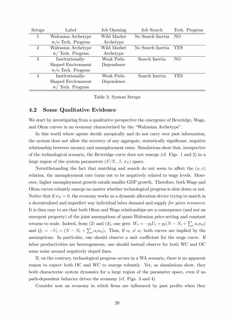
We start by investigating from a qualitative perspective the emergence of Beveridge, Wage,

and Okun curves in an economy characterized by the “Walrasian Archetype”.

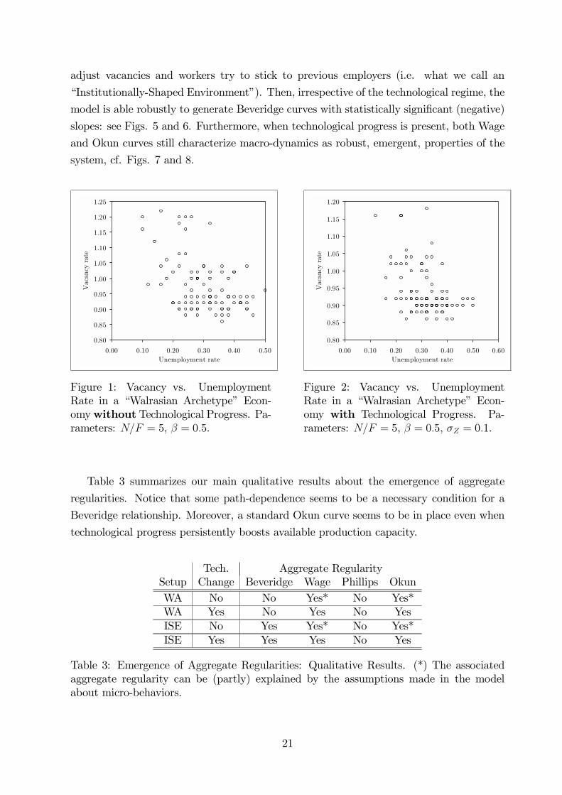
In this world where agents decide myopically and do not carry over past information,

the system does not allow the recovery of any aggregate, statistically significant, negative

relationship between vacancy and unemployment rates. Simulations show that, irrespective

of the technological scenario, the Beveridge curve does not emerge (cf. Figs. 1 and 2) in a

large region of the system parameters (F/N , β, σZ) space.

Notwithstanding the fact that matching and search do not seem to affect the (u, v)

relation, the unemployment rate turns out to be negatively related to wage levels. More-

over, higher unemployment growth entails smaller GDP growth. Therefore, both Wage and

Okun curves robustly emerge no matter whether technological progress is shut down or not.

Notice that if σZ = 0, the economy works as a dynamic allocation device trying to match in

a decentralized and imperfect way individual labor demand and supply for given resources.

It is then easy to see that both Okun and Wage relationships are a consequence (and not an

emergent property) of the joint assumptions of quasi-Walrasian price-setting and constant

returns to scale. Indeed, from (2) and (4), one gets: Wt = −ptUt + pt(N −Nt +P

i αinit)

and Qt = −Ut + (N − Nt +P

i αinit). Thus, if αi 6= α, both curves are implied by the

assumptions. In particular, one should observe a unit coefficient for the wage curve. If

labor productivities are heterogeneous, one should instead observe for both WC and OC

some noise around negatively sloped lines.

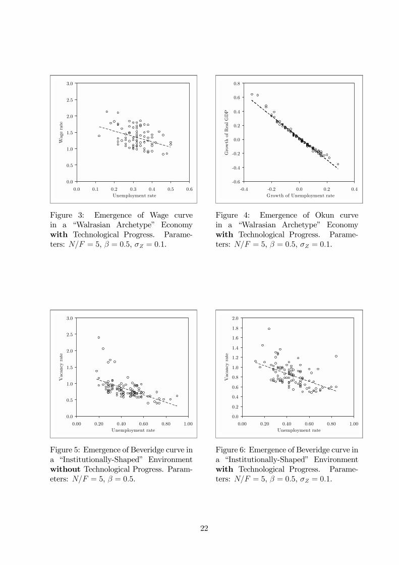
If, on the contrary, technological progress occurs in a WA scenario, there is no apparent

reason to expect both OC and WC to emerge robustly. Yet, as simulations show, they

both characterize system dynamics for a large region of the parameter space, even if no

path-dependent behavior drives the economy (cf. Figs. 3 and 4).

Consider now an economy in which firms are influenced by past profits when they

20

adjust vacancies and workers try to stick to previous employers (i.e. what we call an

“Institutionally-Shaped Environment”). Then, irrespective of the technological regime, the

model is able robustly to generate Beveridge curves with statistically significant (negative)

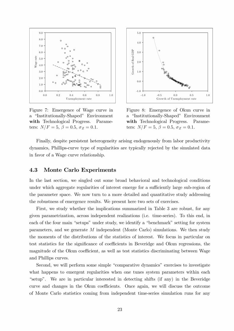
slopes: see Figs. 5 and 6. Furthermore, when technological progress is present, both Wage

and Okun curves still characterize macro-dynamics as robust, emergent, properties of the

system, cf. Figs. 7 and 8.

0.80

0.85

0.90

0.95

1.00

1.05

1.10

1.15

1.20

1.25

0.00 0.10 0.20 0.30 0.40 0.50 Unemployment rate

Vac

ancy

rat

e

Figure 1: Vacancy vs. UnemploymentRate in a “Walrasian Archetype” Econ-omywithoutTechnological Progress. Pa-rameters: N/F = 5, β = 0.5.

0.80

0.85

0.90

0.95

1.00

1.05

1.10

1.15

1.20

0.00 0.10 0.20 0.30 0.40 0.50 0.60 Unemployment rate

Vac

ancy

rat

e

Figure 2: Vacancy vs. UnemploymentRate in a “Walrasian Archetype” Econ-omy with Technological Progress. Pa-rameters: N/F = 5, β = 0.5, σZ = 0.1.

Table 3 summarizes our main qualitative results about the emergence of aggregate

regularities. Notice that some path-dependence seems to be a necessary condition for a

Beveridge relationship. Moreover, a standard Okun curve seems to be in place even when

technological progress persistently boosts available production capacity.

Tech. Aggregate RegularitySetup Change Beveridge Wage Phillips OkunWA No No Yes* No Yes*WA Yes No Yes No YesISE No Yes Yes* No Yes*ISE Yes Yes Yes No Yes

Table 3: Emergence of Aggregate Regularities: Qualitative Results. (*) The associatedaggregate regularity can be (partly) explained by the assumptions made in the modelabout micro-behaviors.

21

0.0

0.5

1.0

1.5

2.0

2.5

3.0

0.0 0.1 0.2 0.3 0.4 0.5 0.6 Unemployment rate

Wag

e ra

te

Figure 3: Emergence of Wage curvein a “Walrasian Archetype” Economywith Technological Progress. Parame-ters: N/F = 5, β = 0.5, σZ = 0.1.

-0.6

-0.4

-0.2

0.0

0.2

0.4

0.6

0.8

-0.4 -0.2 0.0 0.2 0.4 Growth of Unemployment rate

Gro

wth

of R

eal G

DP

Figure 4: Emergence of Okun curvein a “Walrasian Archetype” Economywith Technological Progress. Parame-ters: N/F = 5, β = 0.5, σZ = 0.1.

0.0

0.5

1.0

1.5

2.0

2.5

3.0

0.00 0.20 0.40 0.60 0.80 1.00 Unemployment rate

Vac

ancy

rat

e

Figure 5: Emergence of Beveridge curve ina “Institutionally-Shaped” Environmentwithout Technological Progress. Param-eters: N/F = 5, β = 0.5.

0.0

0.2

0.4

0.6

0.8

1.0

1.2

1.4

1.6

1.8

2.0

0.00 0.20 0.40 0.60 0.80 1.00 Unemployment rate

Vac

ancy

rat

e

Figure 6: Emergence of Beveridge curve ina “Institutionally-Shaped” Environmentwith Technological Progress. Parame-ters: N/F = 5, β = 0.5, σZ = 0.1.

22

0.0

1.0

2.0

3.0

4.0

5.0

6.0

7.0

8.0

9.0

0.0 0.2 0.4 0.6 0.8 1.0 Unemployment rate

Wag

e ra

te

Figure 7: Emergence of Wage curve ina “Institutionally-Shaped” Environmentwith Technological Progress. Parame-ters: N/F = 5, β = 0.5, σZ = 0.1.

-1.0

0.0

1.0

2.0

3.0

4.0

5.0

-1.0 -0.5 0.0 0.5 1.0 Growth of Unemployment rate

Gro

wth

of R

eal G

DP

Figure 8: Emergence of Okun curve ina “Institutionally-Shaped” Environmentwith Technological Progress. Parame-ters: N/F = 5, β = 0.5, σZ = 0.1.

Finally, despite persistent heterogeneity arising endogenously from labor productivity

dynamics, Phillips-curve type of regularities are typically rejected by the simulated data

in favor of a Wage curve relationship.

4.3 Monte Carlo Experiments

In the last section, we singled out some broad behavioral and technological conditions

under which aggregate regularities of interest emerge for a sufficiently large sub-region of

the parameter space. We now turn to a more detailed and quantitative study addressing

the robustness of emergence results. We present here two sets of exercises.

First, we study whether the implications summarized in Table 3 are robust, for any

given parametrization, across independent realizations (i.e. time-series). To this end, in

each of the four main “setups” under study, we identify a “benchmark” setting for system

parameters, and we generate M independent (Monte Carlo) simulations. We then study

the moments of the distributions of the statistics of interest. We focus in particular on

test statistics for the significance of coefficients in Beveridge and Okun regressions, the

magnitude of the Okun coefficient, as well as test statistics discriminating between Wage

and Phillips curves.

Second, we will perform some simple “comparative dynamics” exercises to investigate

what happens to emergent regularities when one tunes system parameters within each

“setup”. We are in particular interested in detecting shifts (if any) in the Beveridge

curve and changes in the Okun coefficients. Once again, we will discuss the outcome

of Monte Carlo statistics coming from independent time-series simulation runs for any

23

given parametrization25.

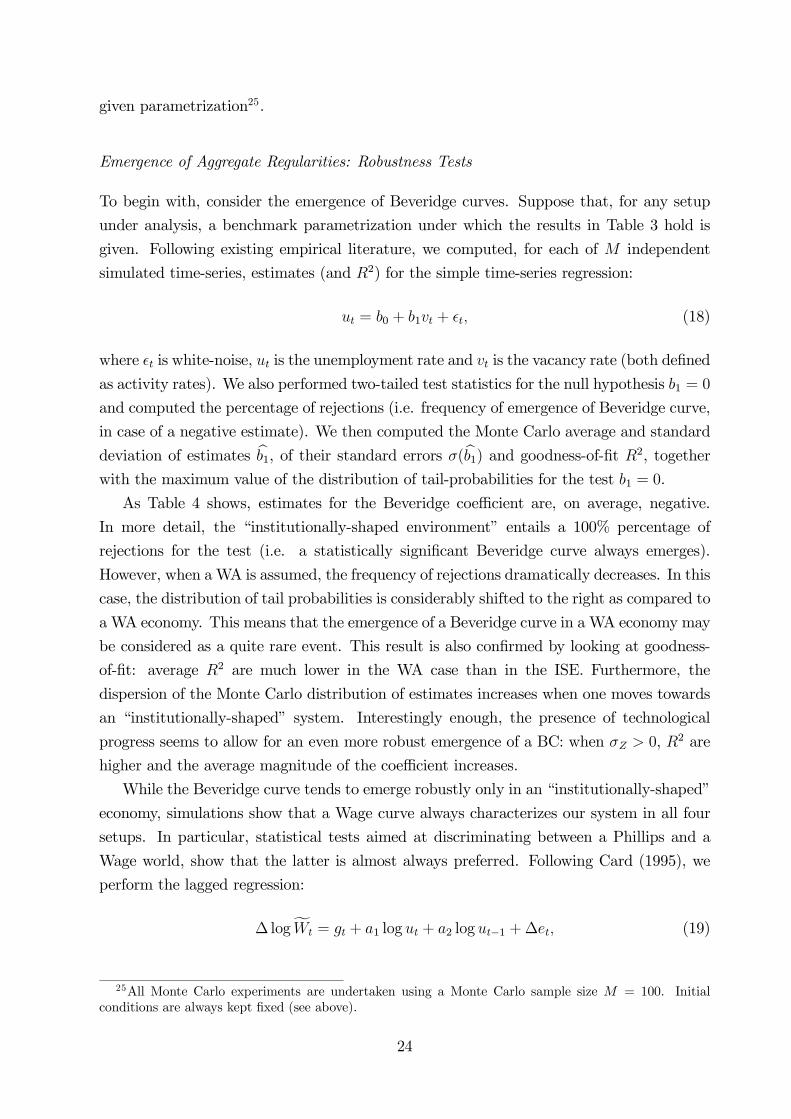
Emergence of Aggregate Regularities: Robustness Tests

To begin with, consider the emergence of Beveridge curves. Suppose that, for any setup

under analysis, a benchmark parametrization under which the results in Table 3 hold is

given. Following existing empirical literature, we computed, for each of M independent

simulated time-series, estimates (and R2) for the simple time-series regression:

ut = b0 + b1vt + $t, (18)

where $t is white-noise, ut is the unemployment rate and vt is the vacancy rate (both defined

as activity rates). We also performed two-tailed test statistics for the null hypothesis b1 = 0

and computed the percentage of rejections (i.e. frequency of emergence of Beveridge curve,

in case of a negative estimate). We then computed the Monte Carlo average and standard

deviation of estimates bb1, of their standard errors σ(bb1) and goodness-of-fit R2, together

with the maximum value of the distribution of tail-probabilities for the test b1 = 0.

As Table 4 shows, estimates for the Beveridge coefficient are, on average, negative.

In more detail, the “institutionally-shaped environment” entails a 100% percentage of

rejections for the test (i.e. a statistically significant Beveridge curve always emerges).

However, when a WA is assumed, the frequency of rejections dramatically decreases. In this

case, the distribution of tail probabilities is considerably shifted to the right as compared to

a WA economy. This means that the emergence of a Beveridge curve in a WA economy may

be considered as a quite rare event. This result is also confirmed by looking at goodness-

of-fit: average R2 are much lower in the WA case than in the ISE. Furthermore, the

dispersion of the Monte Carlo distribution of estimates increases when one moves towards

an “institutionally-shaped” system. Interestingly enough, the presence of technological

progress seems to allow for an even more robust emergence of a BC: when σZ > 0, R2 are

higher and the average magnitude of the coefficient increases.

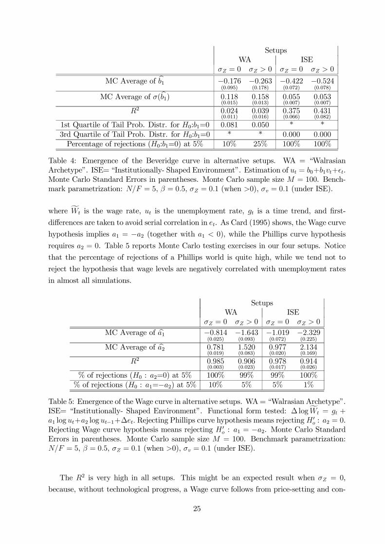
While the Beveridge curve tends to emerge robustly only in an “institutionally-shaped”

economy, simulations show that a Wage curve always characterizes our system in all four

setups. In particular, statistical tests aimed at discriminating between a Phillips and a

Wage world, show that the latter is almost always preferred. Following Card (1995), we

perform the lagged regression:

∆ logfWt = gt + a1 log ut + a2 log ut−1 +∆et, (19)

25All Monte Carlo experiments are undertaken using a Monte Carlo sample size M = 100. Initialconditions are always kept fixed (see above).

24

SetupsWA ISE

σZ = 0 σZ > 0 σZ = 0 σZ > 0

MC Average of bb1 −0.176(0.095)

−0.263(0.178)

−0.422(0.072)

−0.524(0.078)

MC Average of σ(bb1) 0.118(0.015)

0.158(0.013)

0.055(0.007)

0.053(0.007)

R2 0.024(0.011)

0.039(0.016)

0.375(0.066)

0.431(0.082)

1st Quartile of Tail Prob. Distr. for H0:b1=0 0.081 0.050 * *3rd Quartile of Tail Prob. Distr. for H0:b1=0 * * 0.000 0.000

Percentage of rejections (H0:b1=0) at 5% 10% 25% 100% 100%

Table 4: Emergence of the Beveridge curve in alternative setups. WA = “WalrasianArchetype”. ISE= “Institutionally- Shaped Environment”. Estimation of ut = b0+b1vt+$t.Monte Carlo Standard Errors in parentheses. Monte Carlo sample size M = 100. Bench-mark parametrization: N/F = 5, β = 0.5, σZ = 0.1 (when >0), σv = 0.1 (under ISE).

where fWt is the wage rate, ut is the unemployment rate, gt is a time trend, and first-

differences are taken to avoid serial correlation in et. As Card (1995) shows, the Wage curve

hypothesis implies a1 = −a2 (together with a1 < 0), while the Phillips curve hypothesis

requires a2 = 0. Table 5 reports Monte Carlo testing exercises in our four setups. Notice

that the percentage of rejections of a Phillips world is quite high, while we tend not to

reject the hypothesis that wage levels are negatively correlated with unemployment rates

in almost all simulations.

SetupsWA ISE

σZ = 0 σZ > 0 σZ = 0 σZ > 0

MC Average of ba1 −0.814(0.025)

−1.643(0.093)

−1.019(0.072)

−2.329(0.225)

MC Average of ba2 0.781(0.019)

1.520(0.083)

0.977(0.020)

2.134(0.169)

R2 0.985(0.003)

0.906(0.023)

0.978(0.017)

0.914(0.026)

% of rejections (H0 : a2=0) at 5% 100% 99% 99% 100%% of rejections (H0 : a1=−a2) at 5% 10% 5% 5% 1%

Table 5: Emergence of the Wage curve in alternative setups. WA = “Walrasian Archetype”.ISE= “Institutionally- Shaped Environment”. Functional form tested: ∆ logfWt = gt +a1 log ut+a2 log ut−1+∆et. Rejecting Phillips curve hypothesis means rejectingH 0

o : a2 = 0.Rejecting Wage curve hypothesis means rejecting H 0

o : a1 = −a2. Monte Carlo StandardErrors in parentheses. Monte Carlo sample size M = 100. Benchmark parametrization:N/F = 5, β = 0.5, σZ = 0.1 (when >0), σv = 0.1 (under ISE).

The R2 is very high in all setups. This might be an expected result when σZ = 0,

because, without technological progress, a Wage curve follows from price-setting and con-

25

stant returns. However, when σZ > 0, the goodness-of-fit remains high (and standard errors

very low). Our model seems to allow for well-behaved Wage curves also when technological

progress induces persistent heterogeneity in labor productivity dynamics. Furthermore, a

quite general and robust result (see also below) concerns the effect of technological progress

upon the slope of the curve. As discussed above, the latter is expected to be around −1.0when σZ = 0, but nothing can in principle be said about the expected slope when σZ > 0.

Our results suggest that, even when technological progress is present, the Wage curve ro-

bustly emerges. Indeed, wage rates become even more responsive to unemployment than

in the σZ = 0 case.

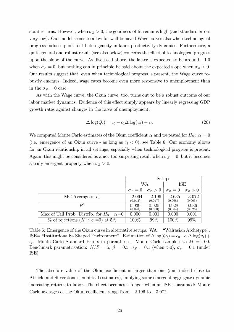
As with the Wage curve, the Okun curve, too, turns out to be a robust outcome of our

labor market dynamics. Evidence of this effect simply appears by linearly regressing GDP

growth rates against changes in the rates of unemployment:

∆ log(Qt) = c0 + c1∆ log(ut) + $t. (20)

We computed Monte Carlo estimates of the Okun coefficient c1 and we tested forH0 : c1 = 0

(i.e. emergence of an Okun curve - as long as c1 < 0), see Table 6. Our economy allows

for an Okun relationship in all settings, especially when technological progress is present.

Again, this might be considered as a not-too-surprising result when σZ = 0, but it becomes

a truly emergent property when σZ > 0.

SetupsWA ISE

σZ = 0 σZ > 0 σZ = 0 σZ > 0

MC Average of bc1 −2.064(0.042)

−2.196(0.047)

−2.635(0.068)

−3.072(0.063)

R2 0.939(0.026)

0.925(0.060)

0.928(0.064)

0.936(0.025)

Max of Tail Prob. Distrib. for H0 : c1=0 0.000 0.001 0.000 0.001% of rejections (H0 : c1=0) at 5% 100% 99% 100% 99%

Table 6: Emergence of the Okun curve in alternative setups. WA = “Walrasian Archetype”.ISE= “Institutionally- Shaped Environment”. Estimation of∆ log(Qt) = c0+c1∆ log(ut)+$t. Monte Carlo Standard Errors in parentheses. Monte Carlo sample size M = 100.Benchmark parametrization: N/F = 5, β = 0.5, σZ = 0.1 (when >0), σv = 0.1 (underISE).

The absolute value of the Okun coefficient is larger than one (and indeed close to

Attfield and Silverstone’s empirical estimates), implying some emergent aggregate dynamic

increasing returns to labor. The effect becomes stronger when an ISE is assumed: Monte

Carlo averages of the Okun coefficient range from −2.196 to −3.072.

26

Notice that one did not assume any increasing returns regime at the individual firm

level. In fact, firms produce using constant returns production functions; see (2). More-

over, no Phillips curve relationships is in place: our economy typically displays a negative

relationship between unemployment rates and wage levels. This suggests that aggregation

of imperfect and persistently heterogeneous behaviors leads to macro-economic dynamic

properties that were not present at the individual level. Therefore, aggregate dynamic

increasing returns emerge as the outcome of aggregation of dynamic, interdependent, mi-

croeconomic patterns (Forni and Lippi, 1997).

Some Comparative Dynamics Monte Carlo Exercises

We turn now to a comparative dynamics Monte Carlo investigation of the effect of system

parameters on emergent aggregate regularities. We focus on the “institutionally-shaped”

setup, wherein the economy robustly exhibits well-behaved Beveridge, Wage, and Okun

curves, and we study what happens under alternative parameter settings. In particular,

we compare parameter setups characterized by:

1. low vs. high N/F ratio (i.e. degrees of concentration of economic activity);

2. low vs. high σv (i.e. sensitivity to market signals in the way firms set their vacancies);

3. low vs. high β (i.e. firms’ bargaining strength in wage setting);

4. low vs. high σZ (technological opportunities).

We first ask whether a higher sensitivity to market signals in vacancy setting induce de-

tectable shifts in aggregate regularities. As Table 7 shows, the smaller σv, the stronger the

revealed increasing dynamic returns: GDP growth becomes more responsive to unemploy-

ment growth and the Okun curve becomes steeper. Notice that σv can also be interpreted

as an inverse measure of path-dependence in firms’ vacancy setting. The smaller σv, the

more firms tend to stick to last-period job openings. Therefore, a smaller path-dependence

implies a steeper Okun relation.

Analogously, we investigate the impact on the BC of simultaneously increasing N/F

(i.e. increasing N for a given F ) and σv (i.e. firms’ “sensitivity to market signals”). Notice

that a higher concentration allows firms, ceteris paribus, to more easily fill their vacancies.

Similarly, the higher σv, the more firms are able to react to aggregate conditions and

correspondingly adjust vacancies. Therefore, one might be tempted to interpret economies

characterized by high values for both N/F and σv as “low friction” worlds, and expect the

BC curve to lie closer to the axes. Notice, however, that, in our model, an “indirect” effect is

also present. If labor demand is very low (e.g. because the economy is in a recession), then

the unemployment rate might be high, irrespective of the value of N/F . Moreover, if σv is

27

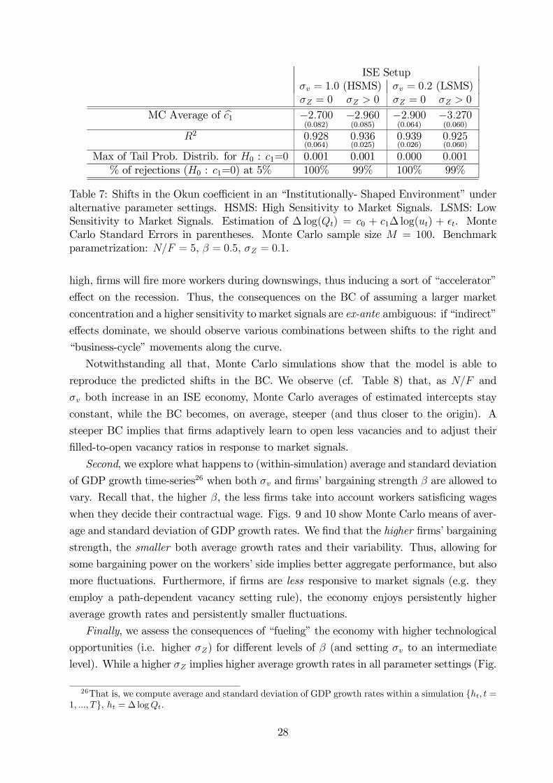
ISE Setupσv = 1.0 (HSMS) σv = 0.2 (LSMS)σZ = 0 σZ > 0 σZ = 0 σZ > 0

MC Average of bc1 −2.700(0.082)

−2.960(0.085)

−2.900(0.064)

−3.270(0.060)

R2 0.928(0.064)

0.936(0.025)

0.939(0.026)

0.925(0.060)

Max of Tail Prob. Distrib. for H0 : c1=0 0.001 0.001 0.000 0.001% of rejections (H0 : c1=0) at 5% 100% 99% 100% 99%

Table 7: Shifts in the Okun coefficient in an “Institutionally- Shaped Environment” underalternative parameter settings. HSMS: High Sensitivity to Market Signals. LSMS: LowSensitivity to Market Signals. Estimation of ∆ log(Qt) = c0 + c1∆ log(ut) + $t. MonteCarlo Standard Errors in parentheses. Monte Carlo sample size M = 100. Benchmarkparametrization: N/F = 5, β = 0.5, σZ = 0.1.

high, firms will fire more workers during downswings, thus inducing a sort of “accelerator”

effect on the recession. Thus, the consequences on the BC of assuming a larger market

concentration and a higher sensitivity to market signals are ex-ante ambiguous: if “indirect”

effects dominate, we should observe various combinations between shifts to the right and

“business-cycle” movements along the curve.

Notwithstanding all that, Monte Carlo simulations show that the model is able to

reproduce the predicted shifts in the BC. We observe (cf. Table 8) that, as N/F and

σv both increase in an ISE economy, Monte Carlo averages of estimated intercepts stay

constant, while the BC becomes, on average, steeper (and thus closer to the origin). A

steeper BC implies that firms adaptively learn to open less vacancies and to adjust their

filled-to-open vacancy ratios in response to market signals.

Second, we explore what happens to (within-simulation) average and standard deviation

of GDP growth time-series26 when both σv and firms’ bargaining strength β are allowed to

vary. Recall that, the higher β, the less firms take into account workers satisficing wages

when they decide their contractual wage. Figs. 9 and 10 show Monte Carlo means of aver-

age and standard deviation of GDP growth rates. We find that the higher firms’ bargaining

strength, the smaller both average growth rates and their variability. Thus, allowing for

some bargaining power on the workers’ side implies better aggregate performance, but also

more fluctuations. Furthermore, if firms are less responsive to market signals (e.g. they

employ a path-dependent vacancy setting rule), the economy enjoys persistently higher

average growth rates and persistently smaller fluctuations.

Finally, we assess the consequences of “fueling” the economy with higher technological

opportunities (i.e. higher σZ) for different levels of β (and setting σv to an intermediate

level). While a higher σZ implies higher average growth rates in all parameter settings (Fig.

26That is, we compute average and standard deviation of GDP growth rates within a simulation {ht, t =1, ..., T}, ht = ∆ logQt.

28

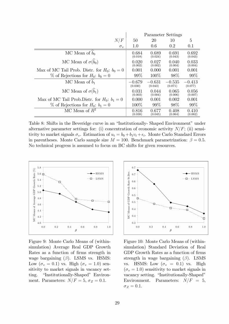
Parameter SettingsN/F 50 20 10 5σv 1.0 0.6 0.2 0.1

MC Mean of bb0 0.684(0.018)

0.689(0.024)

0.691(0.043)

0.692(0.043)

MC Mean of σ(bb0) 0.020(0.002)

0.027(0.002)

0.040(0.004)

0.033(0.004)

Max of MC Tail Prob. Distr. for H0: b0 = 0 0.001 0.000 0.001 0.001% of Rejections for H0: b0 = 0 99% 100% 98% 99%

MC Mean of bb1 −0.679(0.030)

−0.631(0.043)

−0.535(0.071)

−0.413(0.077)

MC Mean of σ(bb1) 0.031(0.003)

0.044(0.004)

0.065(0.006)

0.056(0.007)

Max of MC Tail Prob.Distr. for H0: b1 = 0 0.000 0.001 0.002 0.001% of Rejections for H0: b1 = 0 100% 99% 98% 99%

MC Mean of R2 0.816(0.038)

0.677(0.045)

0.408(0.064)

0.410(0.062)

Table 8: Shifts in the Beveridge curve in an “Institutionally- Shaped Environment” underalternative parameter settings for: (i) concentration of economic activity N/F ; (ii) sensi-tivity to market signals σv. Estimation of ut = b0+ b1vt+ $t. Monte Carlo Standard Errorsin parentheses. Monte Carlo sample size M = 100. Benchmark parametrization: β = 0.5.No technical progress is assumed to focus on BC shifts for given resources.

4.0

4.2

4.4

4.6

4.8

5.0

5.2

5.4

5.6

5.8

0.0 0.2 0.4 0.6 0.8 1.0β

MC

Mea

ns

of A

vera

ge G

DP

Gro

wth

Rat

e (%

)

HSMS

LSMS

Figure 9: Monte Carlo Means of (within-simulation) Average Real GDP GrowthRates as a function of firms strength inwage bargaining (β). LSMS vs. HSMS:Low (σv = 0.1) vs. High (σv = 1.0) sen-sitivity to market signals in vacancy set-ting. “Institutionally-Shaped” Environ-ment. Parameters: N/F = 5, σZ = 0.1.

0.3

0.4

0.4

0.5

0.5

0.6

0.6

0.7

0.7

0.0 0.2 0.4 0.6 0.8 1.0β

MC

Mea

ns o

f G

DP

Gro

wth

Rat

e St

.Dev

.

HSMS

LSMS

Figure 10: Monte Carlo Means of (within-simulation) Standard Deviation of RealGDP Growth Rates as a function of firmsstrength in wage bargaining (β). LSMSvs. HSMS: Low (σv = 0.1) vs. High(σv = 1.0) sensitivity to market signals invacancy setting. “Institutionally-Shaped”Environment. Parameters: N/F = 5,σZ = 0.1.

29

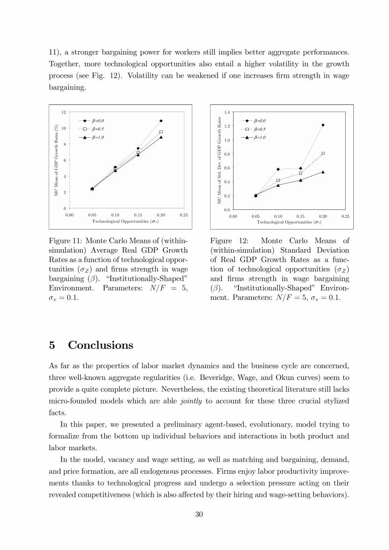
11), a stronger bargaining power for workers still implies better aggregate performances.

Together, more technological opportunities also entail a higher volatility in the growth

process (see Fig. 12). Volatility can be weakened if one increases firm strength in wage

bargaining.

0

2

4

6

8

10

12

0.00 0.05 0.10 0.15 0.20 0.25

Technological Opportunities (σ z)

MC

Mea

n of

GD

P G

row

th R

ates

(%

)

β=0.0

β=0.5

β=1.0

Figure 11: Monte Carlo Means of (within-simulation) Average Real GDP GrowthRates as a function of technological oppor-tunities (σZ) and firms strength in wagebargaining (β). “Institutionally-Shaped”Environment. Parameters: N/F = 5,σv = 0.1.

0.0

0.2

0.4

0.6

0.8

1.0

1.2

1.4

0.00 0.05 0.10 0.15 0.20 0.25Technological Opportunities (σ z)

MC

Mea

n of

Std

. D

ev. o

f G

DP

Gro

wth

Rat

es β=0.0

β=0.5

β=1.0

Figure 12: Monte Carlo Means of(within-simulation) Standard Deviationof Real GDP Growth Rates as a func-tion of technological opportunities (σZ)and firms strength in wage bargaining(β). “Institutionally-Shaped” Environ-ment. Parameters: N/F = 5, σv = 0.1.

5 Conclusions

As far as the properties of labor market dynamics and the business cycle are concerned,

three well-known aggregate regularities (i.e. Beveridge, Wage, and Okun curves) seem to

provide a quite complete picture. Nevertheless, the existing theoretical literature still lacks

micro-founded models which are able jointly to account for these three crucial stylized

facts.

In this paper, we presented a preliminary agent-based, evolutionary, model trying to

formalize from the bottom up individual behaviors and interactions in both product and

labor markets.

In the model, vacancy and wage setting, as well as matching and bargaining, demand,

and price formation, are all endogenous processes. Firms enjoy labor productivity improve-

ments thanks to technological progress and undergo a selection pressure acting on their

revealed competitiveness (which is also affected by their hiring and wage-setting behaviors).

30

Simulations show that the model is able robustly to reproduce Beveridge, Wage and

Okun curves under quite broad behavioral and institutional settings. Moreover, the system

generates endogenously an Okun coefficient greater than one (i.e. aggregate dynamic in-

creasing returns) even if individual firms employ production functions exhibiting constant

returns to labor.

Monte Carlo simulations also indicate that statistically detectable shifts in Okun and

Beveridge curves emerge as the result of changes in institutional, behavioral, and techno-

logical parameters. For example, a higher concentration of market activity (i.e. a higher

number of workers per firm) and a higher sensitivity to market signals in firms’ vacancy

setting rules imply Beveridge curves which lie closer to the axes. Finally, the model gener-

ates quite sharp predictions about how the average aggregate performance (and volatility)

of the system change in alternative behavioral, institutional, and technological setups.

Many issues remain to be explored. First, additional Monte Carlo simulation exercises

could be performed to more finely map (e.g. within a given “system setup”) parameters

and aggregate behaviors.

Second, the issue as to whether (and how) heterogeneity is able to affect the emergence

of aggregate regularities might be addressed. For instance, one could explore the effects to

endow workers (resp. firms) with increasingly heterogeneous distributions of reservation

wages (resp. desired ratios of filled to open vacancies). Third, one might investigate the

consequences of assuming alternative matching and bargaining processes to allow for a

richer institutional setting. Finally, the structure of the model might be complicated in

order to investigate economies where jobs last more than one period and firms are able to

transfer profits across time.

ReferencesAghion, P. and P. Howitt (1994), “Growth and Unemployment”, Review of EconomicStudies, 61: 477—494.

Aoki, M. (2003), “A New Model of Output Fluctuation: Ultrametrics, Beveridge Curveand Okun’s Law”, Economics online papers, no. 234, UCLA.

Aoki, M. and H. Yoshikawa (2003), “A Simple Quantity Adjustment Model of EconomicFluctuations and Growth”, in Cowan, R. and N. Jonard (eds.), Heterogeneous Agents,Interaction and Economic Performance. Berlin, Springer.

Ashenfelter, O. and D. Card (eds.) (1999), Handbook of Labor Economics. Volume 3. El-sevier Science, Amsterdam.

Ashenfelter, O. and R. Layard (eds.) (1986), Handbook of Labor Economics. Volume 2.Elsevier Science, Amsterdam.

Attfield, C. and B. Silverstone (1997), “Okun´s coefficient: A comment”, The Review ofEconomics and Statistics, 79: 326—329.

31

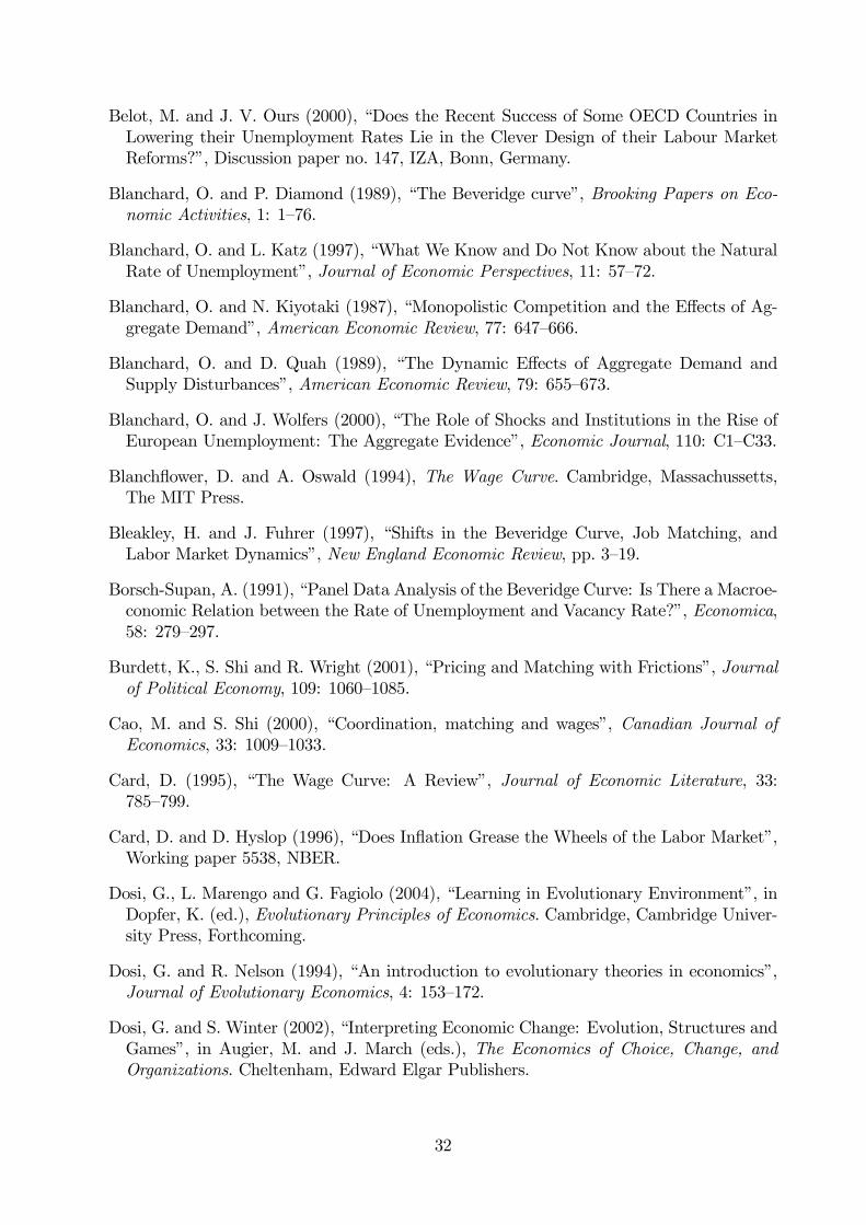
Belot, M. and J. V. Ours (2000), “Does the Recent Success of Some OECD Countries inLowering their Unemployment Rates Lie in the Clever Design of their Labour MarketReforms?”, Discussion paper no. 147, IZA, Bonn, Germany.

Blanchard, O. and P. Diamond (1989), “The Beveridge curve”, Brooking Papers on Eco-nomic Activities, 1: 1—76.

Blanchard, O. and L. Katz (1997), “What We Know and Do Not Know about the NaturalRate of Unemployment”, Journal of Economic Perspectives, 11: 57—72.

Blanchard, O. and N. Kiyotaki (1987), “Monopolistic Competition and the Effects of Ag-gregate Demand”, American Economic Review, 77: 647—666.

Blanchard, O. and D. Quah (1989), “The Dynamic Effects of Aggregate Demand andSupply Disturbances”, American Economic Review, 79: 655—673.

Blanchard, O. and J. Wolfers (2000), “The Role of Shocks and Institutions in the Rise ofEuropean Unemployment: The Aggregate Evidence”, Economic Journal, 110: C1—C33.

Blanchflower, D. and A. Oswald (1994), The Wage Curve. Cambridge, Massachussetts,The MIT Press.

Bleakley, H. and J. Fuhrer (1997), “Shifts in the Beveridge Curve, Job Matching, andLabor Market Dynamics”, New England Economic Review, pp. 3—19.

Borsch-Supan, A. (1991), “Panel Data Analysis of the Beveridge Curve: Is There a Macroe-conomic Relation between the Rate of Unemployment and Vacancy Rate?”, Economica,58: 279—297.

Burdett, K., S. Shi and R. Wright (2001), “Pricing and Matching with Frictions”, Journalof Political Economy, 109: 1060—1085.

Cao, M. and S. Shi (2000), “Coordination, matching and wages”, Canadian Journal ofEconomics, 33: 1009—1033.

Card, D. (1995), “The Wage Curve: A Review”, Journal of Economic Literature, 33:785—799.

Card, D. and D. Hyslop (1996), “Does Inflation Grease the Wheels of the Labor Market”,Working paper 5538, NBER.

Dosi, G., L. Marengo and G. Fagiolo (2004), “Learning in Evolutionary Environment”, inDopfer, K. (ed.), Evolutionary Principles of Economics. Cambridge, Cambridge Univer-sity Press, Forthcoming.

Dosi, G. and R. Nelson (1994), “An introduction to evolutionary theories in economics”,Journal of Evolutionary Economics, 4: 153—172.

Dosi, G. and S. Winter (2002), “Interpreting Economic Change: Evolution, Structures andGames”, in Augier, M. and J. March (eds.), The Economics of Choice, Change, andOrganizations. Cheltenham, Edward Elgar Publishers.

32

Epstein, J. and R. Axtell (1996), Growing Artificial Societies: Social Science from theBottom-Up. Washington D.C., MIT Press.

Evans, G. (1989), “Output and Unemployment Dynamics in the U.S. 1950-1985”, Journalof Applied Econometrics, 4: 213—237.

Fitoussi, J.-P., D. Jestaz, E. Phelps and G. Zoega (2000), “Roots of the Recent Recoveries:Labor Reforms or Provate Secto Forces?”, Brooking Papers on Economic Activities, 1:237—291.

Flaschel, P., G. Kauermann and W. Semmler (2003), “Testing Wage and Price PhillipsCurves for the United States”, Unpublished manuscript, Bielefeld University, Faculty ofEconomics.

Forni, M. and M. Lippi (1997), Aggregation and the Microfoundations of Dynamic Macroe-conomics. Oxford, Clarendon Press.

Hahn, F. and R. Solow (1997), A Critical Essay on Modern Macroeconomic Theory. Cam-bridge, MA, The MIT Press.

Julien, B., J. Kennes and I. King (2000), “Bidding for Labor”, Review of Economic Dy-namics, 3: 619—649.

Kirman, A. (1992), “Whom or what does the representative individual represent ?”, Journalof Economic Perspectives, 6: 117—136.

Laffond, G. and J. Lesourne (2000), “The genesis of expectations and of sunspot equilibria”,Journal of Evolutionary Economics, 2: 211—231.

Lagos, R. (2000), “An Alternative Approach to Search Frictions”, Journal of PoliticalEconomy, 108: 851—872.

Layard, R., R. Jackman and S. Nickell (1991), Unemployment. Oxford University Press,Oxford.

Lesourne, J. (1992), The Economics of Order and Disorder. Oxford, Clarendon Press.

Moosa, I. (1997), “A Cross-Country Comparison of Okun´s Coefficient”, Journal of Com-parative Economics, 24: 335—356.

Mortensen, D. (1986), “Job Search and Labor Market Analysis”, in Ashenfelter, O. andR. Layard (eds.), Handbook of Labor Economics, Volume 2. Amsterdam, Elsevier Science.

Mortensen, D. and C. Pissarides (1994), “Job creation and job destruction in the theoryof unemployment”, Review of Economic Studies, 61: 397—415.

Nickell, S., L. Nunziata, W. Ochell and G. Quintini (2001), “The Beveridge curve, Unem-ployment and wages in the OECD from 1960s to 1990s”, Working paper no. 502, CEPR,London, U.K.

Okun, A. (1962), “Potential GDP: Its Measurement and Significance”, Proceedings of theBusisness and Economics Statistics, pp. 98—103.

33

Okun, A. (1970), The political economy of prosperity. The Brookings Institution, Washing-ton D.C.

Peters, M. (1991), “Ex ante price offers in matching games non-steady states”, Economet-rica, 59: 1425—1454.

Petrongolo, B. and C. Pissarides (2001), “Looking into the Black Box: A Survey on theMatching Function”, Journal of Economic Literature, 39: 390—431.

Phelps, E. (1972), Inflation Policy and Unemployment Theory. MacMillan, London.

Phelps, E. (1994), Structural Slumps. Cambridge, Harvard University Press.

Phelps, E. and S. Winter (1970), “Optimal Price Policy Under Atomistic Competition”, inPhelps, E., G. Archibald and A. Alchian (eds.), Microeconomic Foundations of Employ-ment and Inflation Theory. New York, Norton.

Pissarides, C. (2000), Equilibrium Unemployment Theory. Oxford, Blackwell.

Prachowny, M. (1993), “Okun´s Law: Theoretical Foundations and Revised Estimates”,The Review of Economics and Statistics, 75: 331—336.

Schaik, A. V. and H. D. Groot (1998), “Unemployment and Endogenous Growth”, Labour,12: 189—219.

Shapiro, C. and J. Stiglitz (1984), “Equilibrium Unemployment as a Worker Discipline”,American Economic Review, 74: 1257—78.

Smith, T. and Y. Zenou (2003), “A Discrete-Time Stochastic Model of Job Matching”,Economic Dynamics, 6: 54—79.

Sögner, L. and A. Stiassny (2000), “A Cross-Country Study on Okun´s Law”, Workingpaper no. 13, Vienna University, Faculty of Economics and Business Administration.

Solow, R. (1998), “What is Labour-Market Flexibility? What is it Good for?”, Proceedingsof the British Academy, 97: 189—211.

Tesfatsion, L. (1997), “How Economists Can Get ALife”, in Arthur, W., S. Durlauf andD. Lane (eds.), The Economy as an Evolving Complex System II. Santa Fe Institute,Santa Fe and Reading, MA, Addison-Wesley.

Tesfatsion, L. (2001), “Structure, Behavior, and Market Power in an Evolutionary LaborMarket with Adaptive Search”, Journal of Economic Dynamics and Control, 25: 419—457.

Witt, U. (1985), “Coordination of Individual Economic Activities as an Evolving Processof Self-Organization”, Economie appliquée, 37: 569—595.

34