Towards an integrated coastal sediment dynamics and shoreline response simulator Stephen Pearson, John Rees, Catherine Poulton, Mark Dickson, Mike Walkden, Jim Hall, Robert Nicholls, Mustafa Mokrech, Sotiris Koukoulas and Tom Spencer�� November 2005

Tyndall Centre for Climate Change Research Technical Report 38

Towards an integrated coastal sediment dynamics and shoreline response simulator

Tyndall Centre Technical Report No. 38

November 2005

This is the final report from Tyndall research project T2.45: Towards an integrated coastal-sediment dynamics and shoreline response simulator. The following researchers worked on this project:

Stephen Pearson, John Rees and Catherine Poulton (British Geological Survey) Mark Dickson (NIWA, National Institute of Water and Atmospheric Research, New Zealand) Mike Walkden and Jim Hall (University of Newcastle) Robert Nicholls and Mustafa Mokrech (University of Southampton) Sotiris Koukoulas (University of the Aegean) Tom Spencer (University of Cambridge)

Abstract This report describes a regional scale assessment of coastal erosion undertaken during the period 2000-2100 for a 30-km length of soft-rock coast between Weybourne and Happisburgh, northeast Norfolk. This coastline comprises large lengths of soft, erodible, cliffs, which will be vulnerable to increases in sea level and storminess under future changes in climate. The magnitude of erosion during the next century is of concern to scientists, policymakers and the general public, especially with the expectation of acceleration in sea-level rise. The regional-scale assessment considers combined scenarios of sea-level rise, changing wave climate and coastal management, by successfully integrating a number of modelled elements for the first time. These include: Broad scale modelling of shoreline erosion and profile evolution using the process-based SCAPE (Soft Cliff and Platform Erosion) model; A probabilistic model of cliff-top position derived from SCAPE outputs; and Nearshore wave climate modelling. SCAPE describes the functioning and emergent behaviour of the coastal system at a regional scale, and provides a detailed dataset for analysis of risk and responses to future coastal erosion. The SCAPE model outputs have been linked with a flexible GIS tool (SCAPEGIS), developed to provide visualisation and interpretation of the model results. Outputs are available in the form of maps, dynamic visualisation, and descriptive statistics of key parameters such as cliff toe and cliff top position. It also allows analysis with other datasets such as land use and building location for impact evaluation, and hence could be used in shoreline management and cliff-top land use planning. This research seeks to address a shortfall in coastal erosion research in the UK, whereby analysis of risks and responses to erosion at the coast is hindered by limited knowledge of the size and location of erosion hazard zones. Through the process of considering potential impacts of sea level rise and changing wave climates on rates of soft shore recession a number of questions have been raised concerning the relative importance of shore platform lowering; the extent to which relative sea level rise is controlling continuous cliff retreat; and the nature of the relationship between offshore seabed morphology and coastal evolution. The modelling philosophy adopted by SCAPE offers considerable scope for addressing questions such as these, and thereby provides an important step in improving our understanding of coastal risk from climatic change. Using the approach developed here, planners are provided with a method for examining broad-level system response with combined management and climate-change scenarios. Keywords

Erosion; cliff; sediment dynamics; sea level; GIS

Section 1 - Overview of project work and outcomes

Abstract This report describes a regional scale assessment of coastal erosion undertaken during the period 2000-2100 for a 30-km length of soft-rock coast between Weybourne and Happisburgh, northeast Norfolk. This coastline comprises large lengths of soft, erodible, cliffs, which will be vulnerable to increases in sea level and storminess under future changes in climate. The magnitude of erosion during the next century is of concern to scientists, policymakers and the general public, especially with the expectation of acceleration in sea-level rise. The regional-scale assessment considers combined scenarios of sea-level rise, changing wave climate and coastal management, by successfully integrating a number of modelled elements for the first time:

1. Broad scale modelling of shoreline erosion and profile evolution using the process-based SCAPE (Soft Cliff and Platform Erosion) model;

2. A probabilistic model of cliff-top position derived from SCAPE outputs; 3. Nearshore wave climate modelling.

SCAPE describes the functioning and emergent behaviour of the coastal system at a regional scale, and provides a detailed dataset for analysis of risk and responses to future coastal erosion. The SCAPE model outputs have been linked with a flexible GIS tool (SCAPEGIS), developed to provide visualisation and interpretation of the model results. Outputs are available in the form of maps, dynamic visualisation, and descriptive statistics of key parameters such as cliff toe and cliff top position. It also allows analysis with other datasets such as land use and building location for impact evaluation, and hence could be used in shoreline management and cliff-top land use planning. This research seeks to address a shortfall in coastal erosion research in the UK, whereby analysis of risks and responses to erosion at the coast is hindered by limited knowledge of the size and location of erosion hazard zones. Through the process of considering potential impacts of sea level rise and changing wave climates on rates of soft shore recession a number of questions have been raised concerning the relative importance of shore platform lowering; the extent to which relative sea level rise is controlling continuous cliff retreat; and the nature of the relationship between offshore seabed morphology and coastal evolution. The modelling philosophy adopted by SCAPE offers considerable scope for addressing questions such as these, and thereby provides an important step in improving our understanding of coastal risk from climatic change. Using the approach developed here, planners are provided with a method for examining broad-level system response with combined management and climate-change scenarios. Objectives The main objective of the study was to model the broad characteristics of the coastal system of northeast Norfolk, given a variety of combined climate-change and management scenarios Particular effort is placed on providing quantified predictions of future cliff retreat, because the model is validated on the basis of comparisons of model erosion against rates of shoreline retreat measured from historical maps.

Specific objectives of the study were: 1. To develop a process-based coastal profile evolution model (SCAPE) for integration into the

Tyndall Centre’s Regional Coastal Simulator; 2. To develop scenarios of climate change and coastal management suitable for application to

broad-scale coastal modelling; 3. To develop and demonstrate a methodology for integration and visualisation application of

profile evolution and other coastal data This project is based on the hypothesis that it is possible to develop improved regional scale models of coastal change by integrating broad-scale models of shoreline erosion and profile evolution with scenarios of climate change and coastal management. Work undertaken The SCAPE modelling work was undertaken by Mark Dickson, Mike Walkden and Jim Hall from the University of Newcastle (formerly University of Bristol). Development of the GIS (SCAPEGIS) and subsequent visualisation and interpretation was undertaken by Sotiris Koukoulas, Robert Nicholls and Mustafa Mokrech at the University of Southampton (formerly University of Middlesex). Overall project management, provision of baseline data, and validation of model output were undertaken by Stephen Pearson and John Rees at the British Geological Survey. Tom Spencer at Cambridge University supplied cliff and beach profile data. Results A major innovation of this project has been the integrated analysis of coastal system behaviour, utilizing a scenario-evaluation framework to investigate potential impacts of different climate change and management scenarios Model output was verified through comparison with cliff recession rates measured from historical maps over more than a century along approximately 50 km of coastline. Predictions were then made for the period 2000 to 2100 under combined climatic change and management scenarios. In sensitivity testing, the model is relatively insensitive to increases in offshore wave height, moderately sensitive to changes in wave direction, but highly sensitive to sea-level rise. The coastal response was not simple, however, and under high sea level rise some sectors actually retreated at a lesser rate than under low sea level rise. In all instances the impact of climatic changes on sediment transport patterns were crucially important, with increased rates of erosion in up-drift areas furnishing down-drift sectors with additional sediment, which sometimes had the effect of bulking beaches and decreasing rates of shore platform lowering and cliff recession. This coastal systems model has provided an opportunity to assess coastal response to combined management and climate change scenarios over spatial and temporal scales of particular concern to coastal managers. The effects of different coastal management scenarios indicate that while abandoning cliff defences increases erosion risk, the value of assets at risk for this section of coast is generally about £1 million year-1 in the worst scenario.

Relevance to Tyndall Centre research strategy and overall Centre objectives The research described in this paper is directed towards development of the Tyndall Centre Regional Coastal Simulator (RCS), which aims to provide a coupled suite of process models for investigation of broad scale and long term influences upon the coastal system with a view to informing long term coastal management and adaptation to climate change. This research project integrates with other Tyndall Centre coastal modelling initiatives on the East Anglian coast (for example T2.46), by contributing to the coastal change element of the ‘Integrated Regional Coastal Simulator’ flagship project of Research Theme 4. Work on this project was conducted throughout in close collaboration with Tyndall project T2.46 (Regional assessment of coastal flood risk), utilising common future climate and management scenarios, wave modelling, and GIS platform. Potential for further work Further calibration of SCAPE profile shapes with bathymetric data offshore would be useful to increase confidence in the model. The model’s sensitivity to different rates of change of sea level rise (e.g. linear, non-linear) could also be explored. There is considerable potential for improvement through closer coupling with Regional Climate Models rather than making use of more arbitrary climate change scenarios and sensitivity analyses, such as those described in this study. Seabed sediment transport and broad scale interactions with the rest of the wider coastal system (coastal cell 3) were beyond the scope of this project but could be addressed in future work. Much remains to be learned about possible genetic relationships between historical cliff erosion, longshore and offshore sediment transport, and the evolution of large scale depositional features (such as Winterton Ness and Blakeney Spit) as well as the offshore banks and shoals. As the offshore sandbanks are thought to have a significant control on the coastal wave climate, a sandbank morphological model could be developed to further investigate coastal evolution and erosion for this coastline. Future work could expand the factors considered both in physical and socio-economic terms, with a view to developing robust methods to support broad-scale management of erosion risk. As further scenarios are developed, the SCAPEGIS data sets can be expanded. Further work could be undertaken regarding uncertainty analysis of the predictions of coastal change, with uncertainties more systematically explored. Communication highlights Dickson, M. E., Walkden, M. J. A., Hall, J. W. 2005. Potential impacts of climatic change on the rates of recession of soft rock shores and associated management implications, northeast Norfolk, UK. Climatic Change, in review. Two papers presented at Coastal Dynamics 2005, Barcelona (along with a paper from T2.46), and subsequently published in the conference proceedings:

Dickson, M. E., Walkden, M. J. A., Hall, J. W., Pearson, S.G. and Rees, J. 2005. Numerical modelling of potential climate change impacts on rates of soft cliff recession, northeast Norfolk, UK. Proceedings of Coastal Dynamics 2005, ASCE, New York, in press. Koukoulas S., Nicholls R.J., Dickson M.E., Walkden M.J., Hall J.W., Pearson S.G., Mokrech, M. and Richards, J. 2005. A GIS tool for analysis and interpretation of coastal erosion model outputs (SCAPEGIS). Proceedings of Coastal Dynamics 2005, ASCE, New York, in press. Integrated paper with T2.45, presented at LOICZ II Inaugural Open Science Meeting, Egmond aan Zee, Netherlands: Nicholls R., Brown I., Dawson R., Dickson M., Hall J., Koukoulas S., Mokrech M., Pearson S., Rees J., Richards J., Stansby P., Walkden M., Watkinson A., Zhou J. 2005. An Integrated Assessment of Erosion and Flooding in North-East Norfolk, England. LOICZ II Inaugural Open Science Meeting, Egmond aan Zee, Netherlands, 27-29 June 2005. Five key words/phrases.

Erosion; cliff; sediment dynamics; sea level; GIS

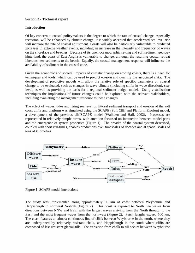
Section 2 - Technical report Introduction Of key concern to coastal policymakers is the degree to which the rate of coastal change, especially recession, will be enhanced by climate change. It is widely accepted that accelerated sea-level rise will increase the rate of coastal adjustment. Coasts will also be particularly vulnerable to predicted increases in extreme weather events, including an increase in the intensity and frequency of waves on the shoreface and beaches. Because of its open oceanographic setting and soft sediment geology hinterland, the coast of East Anglia is vulnerable to change, although the resulting coastal retreat liberates new sediments to the beach. Equally, the coastal management response will influence the availability of sediment in the coastal zone. Given the economic and societal impacts of climatic change on eroding coasts, there is a need for techniques and tools, which can be used to predict erosion and quantify the associated risks. The development of predictive models will allow the relative role of specific parameters on coastal change to be evaluated, such as changes in wave climate (including shifts in wave direction), sea-level, as well as providing the basis for a regional sediment budget model. Using visualisation techniques the implications of future changes could be explored with the relevant stakeholders, including evaluating the management response to those changes. The effect of waves, tides and rising sea level on littoral sediment transport and erosion of the soft coast cliffs and platform was simulated using the SCAPE (Soft Cliff and Platform Erosion) model, a development of the previous cliffSCAPE model (Walkden and Hall, 2002). Processes are represented in relatively simple terms, with attention focussed on interaction between model parts and the emergence of system properties (Figure 1). The breadth of the coastal system described, coupled with short run-times, enables predictions over timescales of decades and at spatial scales of tens of kilometres.

Figure 1. SCAPE model interactions The study was implemented along approximately 30 km of coast between Weybourne and Happisburgh in northeast Norfolk (Figure 2). This coast is exposed to North Sea waves from directions between NNW and ESE, with the largest waves arriving from the North through to the East, and the most frequent waves from the northwest (Figure 2). Fetch lengths exceed 500 km. The coast features an almost continuous line of cliffs between Weybourne in the north, where they are underpinned by relatively resistant chalk, and Happisburgh in the south where cliffs are composed of less resistant glacial-tills. The transition from chalk to till occurs between Weybourne

and Cromer, and broadly coincides with the location of a well-documented drift divide in the direction of longshore sediment transport (Vincent, 1979; Clayton, 1989; Chang and Evans, 1992).

Figure 2 Study area showing main locations, extent of cliffs, model grid, bathymetry, wave directions and sediment transport direction (after Dickson et al., 2005). The direction of sediment transport on the coast is shown in Fig. 1; mainly westward from about Sheringham, and southeast from about Cromer, such that sediment drifts out of both longshore model boundaries. At Sheringham the beach is comprised of shingle above a thin sand layer on top of the underlying chalk platform. The eroding cliffs and shore platform are the main source of sediments to the beaches to the south and east, including the low-lying coast south-east of Happisburgh. Over the course of the 20th Century, coastal structures have been erected to protect the eroding cliffs. This has resulted in a corresponding reduction in sediment supply to the down-drift beaches. On the cliffed coast the inhabited settlements are protected with seawalls, and much of the cliff line was protected with timber palisades (Figure 3) in the 1950s and 60s, which are now reaching the end of their useful life. On the basis of historical maps and photographs as well as records of landmarks and villages that have been lost to the sea, Clayton (1989) estimated that the glacial-till cliffs have retreated at rates averaging around 1 m per year over the past 5000 years, whereas the chalk cliffs have retreated somewhat more slowly. Erosion of soft cliff slopes is sensitive both to marine processes, which can undercut and steepen cliffs, as well as subaerial erosion processes (Lee and Clark, 2002). Primary controls on long-term rates of cliff retreat are the gradient and elevation (relative to sea level) of the shore platform and beach, as these control the ability of waves to remove landslide debris and then attack and destabilise the cliff toe.

SCAPE (Soft Cliff and Platform Erosion) model overview SCAPE is a morphodynamic numerical model that determines the reshaping and retreat of shore profiles along the coast (Walkden & Hall, 2005; Dickson et al., 2005a). Shore recession proceeds through cycles of beach lowering from longshore sediment transport, shore profile erosion, cliff toe retreat and the release of beach sediments from the cliff and platform. In SCAPE, coastal change is determined at 500 m intervals along the coast. A detailed description of SCAPE, including numerical representation of processes and model behaviour has been presented in Walkden and Hall (2005), so detail on model setup is not repeated here. In brief, the model includes representations of the following parameters:

• Wave transformation from nearshore points in the TOMAWAC model, towards the breaker point using linear wave theory;

• Erosion of the shore platform and cliff toe; • Longshore sediment transport using a one-line beach model of the form described in the

Shore Protection Manual (CERC, 1984); • Cross-shore sediment transport using a parameterization of the COSMOS model (Nairn and

Southgate, 1993); • Delivery of talus to the beach; • The effect of shore parallel coastal structures (seawalls and revetments) and groynes.

The shape of the coast, in profile and plan-view, emerges from the dynamic interaction between and within modules, which respond to the imposed loading (waves, tides and sea level rise) and coastal management interventions. While SCAPE uses abstract descriptions, its strength lies in attempting to capture the critical interactions within the entire system, and its stability that is derived through negative feedback, particularly between the behaviour of the beach and shore platform. Cliff-top position is not an output, but is derived offline using a probabilistic model.

Figure 3 Wooden palisades fronting the cliffs at Happisburgh

For the cliffed coastline between Weybourne and Happisburgh, the SCAPE simulations were conducted using a grid based on a series of 63 two-dimensional ‘Y’ sections spaced at 500-m intervals. Shore and beach profile evolution were calculated on the Y sections, whereas bulk longshore sediment transport was calculated halfway between each ‘Y’ section (Dickson et al., 2005). As part of the integration with project T2.46 (Regional assessment of coastal flood risk), the SCAPE modelling was extended beyond the Weybourne to Happisburgh cliffed coast into the low-lying coast as far as Winterton Ness. In this way the effect of up-drift coastal management practices on the down-drift lower-lying coast could be simulated. The results of this analysis are reported in theT2.46 final project report. The SCAPE model is driven by an extended time series of wave heights, periods and direction. The model timestep used was one tidal cycle. At each timestep, forcing conditions were extracted from a time-series of wave and tidal records. Offshore wave heights were hindcast from 23 years of wind records. 13 years of tide gauge data were available. The SCAPE model was driven by extended time series of wave and tide data, so the measured or hindcast time series for these variables were extended to 1000 years, whilst preserving seasonality, by shuffling the 23 time series from the same month each year and preserving the sequence of the months. A representative number of extremes were included in this extended time series by rescaling extremes over a particular threshold to correspond to samples from the estimated extreme value distribution. The distribution of extreme tide levels was obtained from the Proudman Oceanographic Laboratory. A long time series of wave data was required to allow the model to be run long enough for dynamic equilibrium forms to emerge (Walkden and Hall, 2005). The starting condition for each model section was arbitrarily taken to be a vertical cliff plunging into deep water. Through simulation of thousands of years of shore erosion, profiles gradually emerge at each model section. Profile shapes ultimately depend on the cross-shore distribution of erosion, the size of beach (if present), tidal characteristics, material strength, and the incident wave conditions. Erosion is controlled by negative feedback through the form of the beach and platform. Small beaches and steep platforms tend to allow higher rates of erosion. Initially, equilibrium shore profiles were produced assuming waves were not influenced by the topography of offshore banks and shoals (i.e. using shore-parallel isobaths). This was appropriate for capturing the broad long-term characteristics of profiles, but ultimately, over the short and medium term, shoreline processes at northeast Norfolk depend heavily on the offshore topography. To account for these effects, offshore wave data were analysed by Kuang and Stansby (2004) using the TOMOWAC code (part of the EDF TELEMAC suite) which accounts for shoaling, refraction by variable depth and currents, generation by wind, dissipation by whitecapping, bed friction and depth-limited breaking and wave-wave energy transfers, although it doesn’t account for diffraction. The analysis is based upon the assumption that wave propagation inshore is not affected significantly by tidal (or wave-induced) currents, directionality (whether broad or narrow), and wave generation within the coastal domain. This has been previously demonstrated to be valid for this area, although it should be noted that very high wind speeds (greater than about 20m/s) may modify the wave transformation significantly. The coastal domain for the offshore wave modelling extended 30 km off the coast of East Anglia with an alongshore extent of 50-100 km to cover wave propagation from all significant directions. The results of the offshore wave modelling were emulated in a series of nearshore transfer functions spaced along the SCAPE grid. In SCAPE the representation of the resistance of bedrock is treated as a calibration term, established by comparing model predictions of average recession against observed rates. The calibration process begins with a model of the natural, i.e. pre-engineered coast. Different values of resistance were selected to represent the chalk and glacial-till cliffs. The second calibration parameter is the coefficient of longshore sediment transport in the CERC equation, which was set at 0.77 for all model sections on the basis of previous studies of longshore sediment transport on this coast

(Wallingford, 2002). Additional model parameters included representations of the shape of the 15 m isobath, as well as an approximation of the initial, smooth (un-engineered) shoreline plan shape. Initially the model was assumed to be simulating the condition of the shore in a simple “natural” model state without engineering intervention. From a natural, un-engineered state SCAPE was then perturbed to simulate the effects of major historical engineering interventions from the mid 19th Century to the present. The major towns of Sheringham, Cromer, Mundesley and Overstrand have been protected with groynes and seawalls since the latter part of the 19th Century. South of Mundesley, most major engineering works occurred post-1950, with construction largely focussed on the use of groynes and pallisades. In SCAPE seawalls have the effect of preventing cliff toe retreat, but do not stop shore platform lowering. Sloping palisades were simulated by assuming a reduction in the heights of incident waves by 50%, and the effect of groynes by reducing longshore sediment drift until beaches widened to the extent that they bypassed the structures. After simulating the effect of engineering structures on the eroding system between the later part of the 1800s and 2000, model results were compared with historical recession data measured from Ordinance Survey maps. Once a satisfactory validation was achieved, the model was run through combined climate-change and management scenarios to predict shoreline evolution from 2000 to 2100. Model Validation Sediment transport rates, beach volumes and shore platform profile shapes were used as validation to build confidence in the models ability to represent the study site at a regional scale. Modelled longshore sediment transport diverged between Cromer and Weybourne, as has been suggested in a number of studies (e.g. Vincent, 1979; Wallingford, 2002). There was also an increase southward to approximately Happisburgh, with the magnitude of rates being broadly similar to those calculated elsewhere (Wallingford, 2002). South of Happisburgh rates of sediment transport decreased and SCAPE predicted deposition of material on the coastline to the south under natural conditions. This behaviour is generally comparable with the observation that this area historically was associated with sand-dune accumulation (WCHMP, 2003). The reduction in sediment transport potential in this region can be linked through the offshore wave modelling (Kuang and Stansby, 2004) to wave transformation effects that occur across features such as Haisborough Sands. SCAPE shore profiles were compared to bathymetric surveys and hydrographic charts. In general, the modelled profiles appear to be shallower than the bathymetric data indicate. This may be attributable to the lack of representation of tidal currents within SCAPE, as currents in the area are known to be very strong (Wallingford, 2002a) and may, over an extended period, contribute to downwearing of shore profiles. Despite this, the plan-shape variability in SCAPE profiles is broadly comparable to that observed in reality. In particular, profiles are steeper in the north where more resistant chalk cliffs occur, and most gently sloping in the convex area of coast that approximately coincides with Foulness, which is an area of shallower water where historical erosion rates have been relatively high. The SCAPE model was validated through plan-shape comparison of model erosion rates against cliff-toe recession measured between 1885 and 2002 from historical Ordnance Survey maps. The The similarity between model output and measurements of historic cliff recession rate over a 117 year period provided the principle source of model confidence. Figure 4 compares modelled cliff-toe recession rates with historical rates extracted from digitised Ordinance Survey maps. Three epochs of maps had complete coverage of the study area; 1885/6, 1950/1, and 2002. The cliff-toe was digitised with an accuracy approaching 5m, and differences in shoreline positions between the three epochs were extracted at a regular spacing of 100 m along the coast. Plan-shape annual

recession rates were then calculated and a moving average obtained across 1500 m of coastline. Despite the uncertainty inherent within measured data and the highly abstracted representation of reality, SCAPE produces erosion rates that are similar to measured rates over the 117-year validation period (Figure 4). The modelling approach is important, in which emphasis is placed on understanding and representing feedback and interactions between system components.

Figure 4 Comparison between SCAPE predictions of shoreline recession and measured rates form Ordnance Survey maps (after Dickson et al. 2005) In contrast to the cliffed coastline, less confidence was obtained at the model boundary regions, where the cliffs are replaced by low-lying unconsolidated landforms. Since the cliff baseline is absent on the maps from these areas as a marker of shoreline position, it is more difficult to compare model predictions, but figure 4 includes a comparison of the Mean High Water level represented on the Ordnance Survey maps with the still water level output from SCAPE. This illustrates that further work is required to improve the representation description of interactions along unconsolidated coasts. Effect of engineering works on shoreline recession The degree of similarity between model output and measurements of cliff recession highlights the significant effect that structures have on the system. For example, the impact of engineering works is clear in Figure 4, where seawalls at Cromer and Sheringham have prevented cliff-toe erosion, in

contrast to the undefended coast between Overstrand and Trimmingham which has eroded more rapidly. There are also more subtle effects, for example on the distribution of beach-forming sediments and the relative level of shore platforms, which need to be considered when appraising the overall impact of defence schemes. When SCAPE simulates a natural coastline, the average sediment flux at Happisburgh near the southern end of the cliff section approaches 400,000 m3yr-1

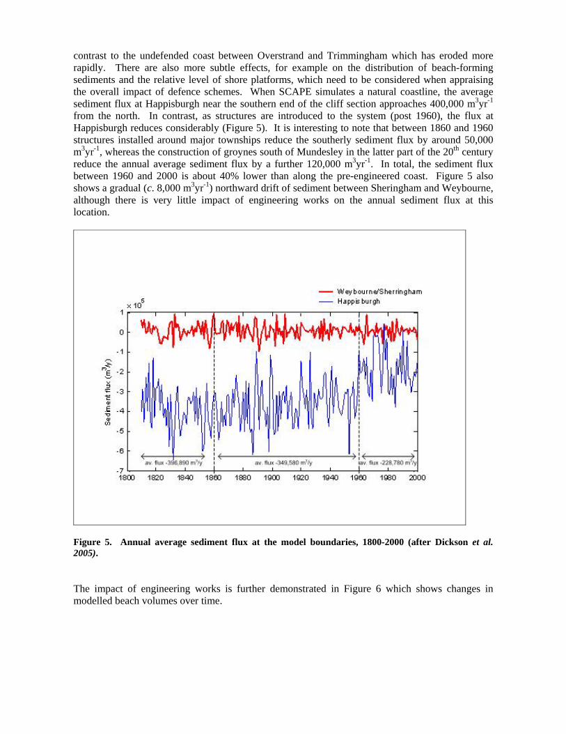
from the north. In contrast, as structures are introduced to the system (post 1960), the flux at Happisburgh reduces considerably (Figure 5). It is interesting to note that between 1860 and 1960 structures installed around major townships reduce the southerly sediment flux by around 50,000 m3yr-1, whereas the construction of groynes south of Mundesley in the latter part of the 20th century reduce the annual average sediment flux by a further 120,000 m3yr-1. In total, the sediment flux between 1960 and 2000 is about 40% lower than along the pre-engineered coast. Figure 5 also shows a gradual (c. 8,000 m3yr-1) northward drift of sediment between Sheringham and Weybourne, although there is very little impact of engineering works on the annual sediment flux at this location.

Figure 5. Annual average sediment flux at the model boundaries, 1800-2000 (after Dickson et al. 2005). The impact of engineering works is further demonstrated in Figure 6 which shows changes in modelled beach volumes over time.

Figure 6 Modelled beach volumes, 1800-2000 (after Dickson et al. 2005). It is apparent that under natural conditions the volume of sediment in beaches on the north-facing coast (e.g. Sheringham, Cromer) is small compared with beaches further to the southeast (e.g. Trimmingham, Happisburgh), due to the natural divide in the direction of longshore sediment transport. However, SCAPE predicts that at Cromer the construction of groynes in the latter part of the 19th century resulted in a significant increase in beach volumes, although following this initial perturbation there has since been a gradual decrease in average annual beach volumes. Engineering structures at Sheringham had little effect on average beach volumes and along the relatively un-engineered coast at Trimmingham model beach volumes have also remained constant over time. At Happisburgh the model predicts a marked increase in beach volumes following the construction of groynes in the latter part of the 20th century, although this increase was short-lived as SCAPE predicts low beach volumes at the present day. Field observation during the project concurs with this, showing the maximum intertidal beach thickness at Happisburgh to be of the order of only 0.7-0.9m. Figure 7 shows modelled shore platform profiles at Cromer that lower considerably following the introduction of a seawall in late 19th century. An important consideration is the effect of engineering works on coastal evolution is recognition that while seawalls and palisades may reduce rates of cliff recession, they do not protect the shore platform that fronts them. Lowering of the shore profile is important for potential undermining of defences, but also in that it allows waves to break closer to the cliff toe. Hence, if structures were to fail or be removed, it is expected that subsequent cliff recession would proceed more rapidly than under natural conditions, as beach volumes are likely to be in a depleted state and offer less protection from wave action. The erosive force of waves will be higher due to deeper water at the cliff toe.

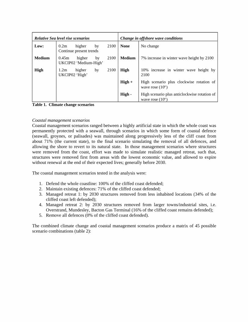
Figure 7. Example of modelled platform lowering (after Dickson et al. 2005). Model validation illustrates that the consequences of the combined effects of platform depression, sediment transport patterns, beach volumes, and changing climate are potentially very important. On the basis of the similarities between the modelled and actual coastline, the next stage was to use the model to make predictions of the likely impacts of management and climate scenarios for the period 2000 to 2100. Scenario testing using Climate change and coastal management scenarios Sea level rise and wave climate scenarios The sea level rise scenarios used in this study were based on reports by the Intergovernmental Panel on Climate Change (IPCC, Church et al., 2001), and UK Climate Impacts Programme (UKCIP02, Hulme et al., 2002). Three sea-level rise scenarios were used (Table 1), each of which included a regional subsidence rate of 0.7 mm yr-1 (Shennan and Horton, 2002). The ‘low’ relative sea–level rise is a constant 2 mm yr-1 (or 0.2m by 2100), which simulates no anthropogenic influence and continues observed trends (Woodworth et al., 1999). The ‘medium’ scenario follows the UKCIP02 medium-high scenario, and results in an increase of 0.45 m by 2100. The ‘high’ scenario is based on the IPCC high limit, plus a regional sensitivity value of +50% to allow for possible spatial variability in thermal expansion (Gregory et al., 2001). This scenario results in increased sea level relative to 2000 levels of 1.2 m by 2100. Model sensitivity to changes in wave climate was investigated by linearly increasing winter offshore wave heights. In the ‘low’ scenario there was no change in offshore wave heights, whereas offshore winter wave heights were increased linearly in the ‘medium’ and ‘high’ scenarios up to a maximum of 7% and 10% respectively by 2100. In addition to these scenarios, +10º (clockwise) and –10 º (anticlockwise) shifts in the offshore wave rose were applied to explore sensitivity to offshore wave direction. The potential impacts of changing storm surge and wave period were not considered.

Relative Sea level rise scenarios

Change in offshore wave conditions

Low: 0.2m higher by 2100 Continue present trends

None No change

Medium 0.45m higher by 2100UKCIP02 ‘Medium-High’

Medium 7% increase in winter wave height by 2100

High 1.2m higher by 2100UKCIP02 ‘High’

High 10% increase in winter wave height by 2100

High + High scenario plus clockwise rotation of wave rose (10°)

High - High scenario plus anticlockwise rotation of wave rose (10°)

Table 1. Climate change scenarios Coastal management scenarios Coastal management scenarios ranged between a highly artificial state in which the whole coast was permanently protected with a seawall, through scenarios in which some form of coastal defence (seawall, groynes, or palisades) was maintained along progressively less of the cliff coast from about 71% (the current state), to the final scenario simulating the removal of all defences, and allowing the shore to revert to its natural state. In those management scenarios where structures were removed from the coast, effort was made to simulate realistic managed retreat, such that, structures were removed first from areas with the lowest economic value, and allowed to expire without renewal at the end of their expected lives; generally before 2030. The coastal management scenarios tested in the analysis were:

1. Defend the whole coastline: 100% of the cliffed coast defended; 2. Maintain existing defences: 71% of the cliffed coast defended; 3. Managed retreat 1: by 2030 structures removed from less inhabited locations (34% of the

cliffed coast left defended); 4. Managed retreat 2: by 2030 structures removed from larger towns/industrial sites, i.e.

Overstrand, Mundesley, Bacton Gas Terminal (16% of the cliffed coast remains defended); 5. Remove all defences (0% of the cliffed coast defended).

The combined climate change and coastal management scenarios produce a matrix of 45 possible scenario combinations (table 2):

Relative sea-level rise scenario (2000 to 2100)

Low (0.2m rise)

Medium (0.45m rise)

High (1.2m rise)

Management Scenario (% of cliffed coast protected)

Hs l

ow

(no

chan

ge)

Hs h

igh

(+

10%

)

Hs h

igh

+

(+10

%

&

+10o )

Hs h

igh

–

(+10

% &

-10

o )

Hs

mid

(+7%

)

Hs l

ow

(no

chan

ge)

Hs h

igh

(+10

%)

Hs h

igh

+ (+

10%

& +

10o )

Hs h

igh

– (+

10%

& -

10o )

1 (100%) 1 2 3 4 5 6 7 8 9 2 (71%) 10 11 12 13 14 15 16 17 18 3 (34%) 19 20 22 23 24 25 26 27 4 (16%) 28 29 30 31 32 33 34 35 36 5 (0%) 37 38 39 40 41 42 43 44 45

Table 2. Summary of the 45 climate change (relative sea-level rise, wave ht (Hs) and direction) and management scenarios used in the analysis.

Results of SCAPE modelling Modelled impacts of climate change, 2000-2100: Figure 8 shows average annual recession rates for the period 2000-2100 on an unmodified coast but which has been subject to three different sea-level rise scenarios. The figure demonstrates that SCAPE predicts a relatively complex plan-shape response of shoreline recession to accelerated sea-level rise. Under natural conditions (prior to engineering works) erosion rates are highest between Cromer and Overstrand and decrease to the north, where there are more resistant rocks, and south where beach volumes are higher. The medium SLR scenario has a relatively minor effect on recession rates, but high SLR results in substantial increases (c. 40%) in erosion rates from Overstrand north, moderate increases between Bacton and Overstrand (c. 10%), and decreased recession between Bacton and the southern limit of cliffs near Eccles (c. -10%).

Figure 8. SCAPE model output under different sea level scenarios for the period 2000-2100. The changes in erosion rates along the pre-engineered coast can be attributed to the interaction between erosion and subsequent redistribution of sediments alongshore; however the gradient of sediment transport increases steadily southward toward Bacton, and then flattens markedly. This reduction in gradient results in sediment deposition south of Bacton, which significantly increases

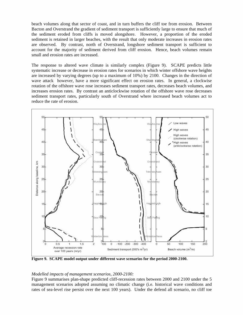
beach volumes along that sector of coast, and in turn buffers the cliff toe from erosion. Between Bacton and Overstrand the gradient of sediment transport is sufficiently large to ensure that much of the sediment eroded from cliffs is moved alongshore. However, a proportion of the eroded sediment is retained in larger beaches, with the result that only moderate increases in erosion rates are observed. By contrast, north of Overstrand, longshore sediment transport is sufficient to account for the majority of sediment derived from cliff erosion. Hence, beach volumes remain small and erosion rates are increased. The response to altered wave climate is similarly complex (Figure 9). SCAPE predicts little systematic increase or decrease in erosion rates for scenarios in which winter offshore wave heights are increased by varying degrees (up to a maximum of 10%) by 2100. Changes in the direction of wave attack however, have a more significant effect on erosion rates. In general, a clockwise rotation of the offshore wave rose increases sediment transport rates, decreases beach volumes, and increases erosion rates. By contrast an anticlockwise rotation of the offshore wave rose decreases sediment transport rates, particularly south of Overstrand where increased beach volumes act to reduce the rate of erosion.

Figure 9. SCAPE model output under different wave scenarios for the period 2000-2100. Modelled impacts of management scenarios, 2000-2100: Figure 9 summarises plan-shape predicted cliff-recession rates between 2000 and 2100 under the 5 management scenarios adopted assuming no climatic change (i.e. historical wave conditions and rates of sea-level rise persist over the next 100 years). Under the defend all scenario, no cliff toe

recession could occur, but the average level of the shore platform close to the cliff toe is predicted to drop in most places by about 2 m in comparison with 2000 levels. Under the “maintain existing defences” scenario coastal towns are defended, but sediments are released from areas with little defence between towns, such that shore profile lowering is not as rapid as under the ‘defend all’ scenario. In general, areas with little defence between Cromer and Overstrand, Overstrand and Trimmingham as well as around Happisburgh, erode between 80 and 100 m during the periodand suffer little profile lowering, whereas the profile lowers by 1 to 1.5 m around towns as well as along the low-lying coast south of Happisburgh (which is protected in all strategies by a seawall). It is notable that under current practices, SCAPE predicts that the coast between Trimmingham and Mundesley and between Mundesley and Bacton will erode at about half the rate of other areas owing to the buffering effect of sediment eroded from updrift sectors. The rapidly eroding coast around Happisburgh receives some benefit from sediment arriving from the north, but this may not be sufficient to compensate for the fact that collapse of structures during the 1990s exposed a coast that had previously been pushed far from its natural equilibrium state, and which is attempting to retain this profile by retreating at an accelerated rate. This is apparent in the figure representing recession stages, with coastal recession at Happisburgh predicted to be most rapid in the first 25 years of the 21st century. This modelled state is currently being experience in the real world at Happisburgh, with rapid erosion of the non-defended coastline immediately to the south. Under “managed retreat scenario 2”, in which structures are retained in front of major towns and Bacton Gas Terminal, but removed from all other areas at the end of their residual lives (c. 20-30 years), markedly increased erosion rates are observed between Trimmingham and Mundesley, as well as between Mundesley and Happisburgh. The large volume of additional sediment that is released has an immediate impact on reducing erosion near Happisburgh by a total of c. 20 to 30 m. Some proportion of this released material also accumulates in beaches south of Happisburgh and so reduces the rate of platform lowering in this area. Under “managed retreat scenario 1” in which the towns of Cromer and Sheringham remain protected while other structures are removed at the end of their effective lives, very high erosion rates (> 120 m) occur at the towns of Overstrand and Mundesley. These towns have been protected for a long time and are therefore far from their natural state. Rapid erosion at these locations reduces erosion rates between Mundesley and Happisburgh by about one third (c. 30 m less erosion over 100 years), and leads to an increase in the relative platform elevation but this benefit is not significant south of Bacton. Finally, under the “remove all defences” scenario there is little benefit to the remainder of the coastal system in terms of reducing erosion rates and rates of platform lowering. A major reason for this is that a large proportion of the sediment liberated by erosion at Cromer and Sheringham is moved westwards by longshore drift. Climate change and management intervention combined: Figure 10 summarises the increase in coastline recession predicted under combined climate change and management scenarios:

Figure 10. SCAPE model output under combined climate and management scenarios

With increased offshore winter wave height there is little systematic change in erosion rates under the three management scenarios. An exception to this is that under management scenario 2 (“managed retreat 1”), increased wave heights give rise to up to 20 m of additional erosion between Bacton and Happisburgh. Changes in offshore wave direction have a greater impact than increased wave heights. A 10-degree clockwise rotation in the offshore wave rose typically increases erosion rates at all sections alongshore, whereas a 10-degree anticlockwise rotation typically decreases erosion rates alongshore. There is some variability in the degree to which changes in offshore wave direction are important. For instance, changes in erosion rates tend to be more pronounced in the vicinity of Trimmingham than further south near Happisburgh. Figure 10 demonstrates that for the 45 scenarios tested, sea-level rise exerts a more significant impact on erosion rates than changes in offshore wave conditions. These effects are likely to be most pronounced from Overstrand north, where increased recession rates of 40-60 m occur between 2000 and 2100. Along the same sector of coast, changes in offshore wave conditions account for changes in recession rate of generally less than 10 m. South of Overstrand, increases in erosion rates under high sea-level rise scenarios are considerably smaller, with typically less than 20 m increased recession between 2000 and 2100. This behaviour results from the extra sediment released from accelerated erosion further north, making its way into larger beaches south of Mundesley. This effect is particularly pronounced under managed retreat scenario 1, in which structures are removed from much of the cliffed coast. Under this management scenario, high sea-level rise results in little discernable change in erosion rates between Bacton and Happisburgh. It is clear form the above that the results of combined management and climate-change scenario-testing imply a complex interacting set of coastal responses over the 21st Century on the northeast Norfolk coast.

Other modelling work Probabilistic cliff top model SCAPE provides predictions of cliff toe position, so in order to define cliff-top recession and erosion hazard zones, these need to be translated to a cliff-top position. This was accomplished using the probabilistic cliff top model of Hall et al. (2002). This provides probability density functions of cliff top position for any given cliff toe position. Recession distances (from initial cliff toe positions) corresponding to the 5th and 95th percentiles of the probability density function were extracted and used to generate the areas on the cliff top considered to be lost, at risk, and safe (Figure 11). It should be noted that the probability density function of cliff top position accounts only for the uncertainty in the angle of the cliff slope and not for uncertainties in the location of the cliff toe.

Predictions of cliff top recession are generated by taking the SCAPE predictions of cliff toe recession and then sampling, from the relevant distributions, an initial cliff angle and then a sufficiently long sequence of pre and post failure cliff angles (αf and αs). Within a Cliff Behavioural Unit, the cliff can be expected to fail when it reaches a average angle αf and will, after failure, adopt an angle αs). Current mean cliff angle and pre and post failure mean cliff angles and variances were determined for each Cliff behavioural Unit and used as input data to the cliff top model. Cliff angles were determined using a combination of existing BGS cliff data, expert judgment supported by field reconnaissance, and “cleaned” Environment Agency coastal profile data, which was processed as part of the project. The data comprised a time series of data covering 1992-2003. These data were “cleaned” by removing translation errors in the coordinate and profile data, and “harmonised” by extending profiles to a common datum (in this case MLW). Large numbers of samples of these sequences of angles are used to generate a histogram of predicted cliff top locations at given numbers of years in the future (Hall et al. 2002). Visualisation using SCAPEGIS Using GIS technology to visualise coastal erosion predictions provides a powerful means to understand coastal changes and their impact in local and regional scales (Brown et al., 2004).

?Lost At Risk

Cliff Toe

Possible Cliff Tops

95th percentile

5th percentile

Fig. 11. Probablistic model of cliff top position. Areas lost and at risk on the cliff-top are identified. All other areas are considered safe

SCAPEGIS adds visualization and spatial analysis capability to SCAPE and the cliff top prediction models, and as such can be used as an impact analysis and decision support tool. The objectives of developing the SCAPEGIS framework were to:

• Develop a GIS interface for visualisation of SCAPE and cliff top model output; • Integrate SCAPE and cliff top model outputs with other spatial datasets, • Facilitate analysis and decision support.

The main screen of the user interface of SCAPEGIS is shown in Figure 4.

Figure 12 Main user interface within SCAPEGIS Instructions for loading and working with SCAPEGIS, including details of how to read and display cliff top model outputs, are included in appendix 2. SCAPEGIS can be used to visualise data of past and future scenarios of shoreline evolution using a number of outputs from the SCAPE model, as follows:

• Cliff toe position is determined as the total amount of cliff base recession at each model Y section each year;

• Cliff top position is determined from the probablistic cliff top prediction model; • Beach volume is determined by the average volume of sediment held in beaches along 500m

sections of coast at each Y section each year;

• Shore platform level is defined as the average relative level of the shore platform near the cliff toe for each Y section each year;

• Sediment supply is defined as the average amount of sediment added to the beach from cliff and platform erosion at each Y section each year;

• The flux of sediment at the boundaries of the cliffed section is also included. Other spatial data can also be input to SCAPEGIS (e.g. land use, population) for visualisation and impact analysis. The interrelationships between model outputs and SCAPEGIS are shown in Figure 13.

Figure 13 Relationships between SCAPEGIS and model outputs. An “offline” protocol was used to link the SCAPE model and cliff top predictions with the GIS, which means that the model and the GIS tool can be operated separately. The advantage of this method is that it allows for independent development, use and updating of the two tools, although in the future, the SCAPE and cliff-top models could be embedded in the GIS if this was thought to be advantageous. Visualisation is a major element of SCAPEGIS, but the capability of SCAPEGIS extents far beyond just producing maps. The GIS has functions to link back to the SCAPE model, providing information to define the baseline and grid and for validation of results, as well as other spatial information necessary for the model’s operation. It should be noted that the parallel development of SCAPEGIS assisted in the development of the SCAPE model. As well as changes in coastline position and beach state, SCAPEGIS can be used to assess their impacts of on cliff top land use and associated urban areas. If land use and infrastructure data are available, then the types of land use and the level of infrastructure that will be lost or at risk can be

Climate/Management Scenarios

SCAPE model

Model Outputs (mainly SCAPE)

Cliff toe position Cliff top position Beach Volume

Shore platform elevation Sediment Supply

Cliff - top model (probabilistic) Construction

Impact Analysis, Decision Support

SCAPEGIS

Geographic Utility Development

Other Data Land use

Population Scenarios

Climate/Management Scenarios

SCAPE model

Model Outputs (mainly SCAPE)

Cliff toe position Cliff top position Beach Volume

Shore platform elevation Sediment Supply

Cliff - top model (probabilistic) Construction

Impact Analysis, Decision Support

SCAPEGIS

Geographic Utility Development

Other Data Land use

Population Scenarios

estimated. The user of SCAPEGIS can build polygons for each model section to estimate land loss between the cliff top position in the “current” year and at a predicted time in the future (for the purpose of this study up to 2100). It is also possible to estimate land losses in specific areas (for example urban boundaries) by selecting the appropriate sections. Using CORINE land cover maps, it was possible to estimate the type and the amount of land loss during the period 2000 to 2100 under different management scenarios. Using OS Landline and OS Address Layer data it was possible to estimate the number of buildings and residential properties that will be lost or at risk in the next 100 years for each SCAPE scenario. Preliminary economic analyses have also been made, in terms of both undiscounted losses, and the net present value of the losses as determined using the standard national project appraisal methods in England and Wales (Penning-Rowsell et al., 2003; Hall et al., 2000). Outputs from SCAPEGIS Visualisations of coastal recession undertaken for the study area, based on SCAPE output of the different management and climate scenarios. Typical output is shown in figure 14, which highlights the extent of cliff top recession (the risk zone) at 2100 for an extreme scenario under which all defences are removed with high sea level rise and a 10% increase in wave height. Such visualisations can be dramatic, especially in urban areas, and may represent a useful way to communicate potential erosion risk. Fig. 14. Example of SCAPEGIS visualization of estimated cliff-top retreat for 2100. Land seaward of the yellow line is assumed to be lost, while land between the yellow and blue lines is at risk. The loss of land, buildings and residential properties under the 45 climate and management scenarios were calculated. Unsurprisingly, losses increase as the proportion of defended land decreases, although it is also apparent that there are losses even under complete protection, especially land loss. This may reflect uncertainty in the baseline data compared with SCAPE

predictions, and also the linear representation of the coast between the 500-m modelled cross-sections in SCAPEGIS. As the erosion hazard zones are narrow, small errors in position translate into large potential errors in erosion risk. It is also possible for there to be failure even if the cliff toe defences are maintained due to subaerial mass movement processes. An example is the cliff-top failure at Clifton Way, Overstrand, which failed during the 1990’s despite long-term cliff-toe protection. Figure 15 provides an illustration of building and residential property losses, while figure 16 shows the total land and arable land losses, respectively. There are losses under all the cases without full protection, even with the low sea-level rise scenario, which highlights the erosional nature of this coastline. Losses increase with sea-level rise and decreasing protection. Wave scenarios are seen to also influence the losses, but to a lesser degree than the other factors. Land loss and residential property losses show contrasting behaviour. Land loss increases dramatically as the amount of protection declines from 100% protection to 71% protection (maintain existing defences), but land losses do not grow so rapidly with further reductions in protection, although the losses are not necessarily occurring in the same locations. The difference in land losses between the low and high sea-level rise scenarios is approximately 20%. Residential property losses increase as protection decreases, and this effect accelerates as protection falls to zero. The difference in residential property losses between the low and high sea-level rise scenarios is approximately 40%. This difference in land and residential property losses mainly reflects the non-uniform distribution of residential properties. Hence, small additional land losses as defences are abandoned can lead to significant additional residential property losses. The undiscounted value of the residential properties lost along this coastline from 2000-2100 has been calculated at up to £194 million (in 2001 GBP). In terms of net present value, this is up to approximately £1 million/year. These values are incomplete as they do not include non-residential properties or transport link disruption. However, this omission is unlikely to change the overall picture that, while impressive when visualised (figure 14), the economic losses on this coastline due to erosion are quite small under the climate change and management scenarios considered here.

Man

agem

ent S

cena

rios

No of Buildings/Properties

12

34

50

500

1000

SLR

hig

hH

s hi

gh

12

34

5

SLR

low

Hs

high

12

34

5

SLR

med

Hs

high

SLR

hig

hH

s hi

gh -

SLR

low

Hs

high

-

0500

1000

SLR

med

Hs

high

-0

500

1000

SLR

hig

hH

s hi

gh +

SLR

low

Hs

high

+S

LR m

edH

s hi

gh +

SLR

hig

hH

s lo

wS

LR lo

wH

s lo

w

0500

1000

SLR

med

Hs

low

0

500

1000

SLR

hig

hH

s m

edS

LR lo

wH

s m

edS

LR m

edH

s m

ed

Bui

ldin

gs.L

ost

Res

iden

tial.P

rope

rties

.Los

t

Fig.

15.

Tot

al n

umbe

r of

bui

ldin

gs a

nd r

esid

entia

l pro

pert

ies l

ost p

er c

limat

e

(sea

leve

l and

wav

e) a

nd m

anag

emen

t sce

nari

o or

the

peri

od 2

000

to 2

100

Fig.

16.

Tot

al la

nd lo

ss a

nd a

rabl

e la

nd lo

ss p

er c

limat

e (s

ea le

vel a

nd w

ave)

and

man

agem

ent s

cena

rio

for

th

e pe

riod

200

0 to

210

0

Man

agem

ent S

cena

rios

Land Area, ha

12

34

5050100

150

200

SLR

hig

hH

s hi

gh

12

34

5

SLR

low

Hs

high

12

34

5

SLR

med

Hs

high

SLR

hig

hH

s hi

gh -

SLR

low

Hs

high

-

050100

150

200

SLR

med

Hs

high

-050100

150

200

SLR

hig

hH

s hi

gh +

SLR

low

Hs

high

+S

LR m

edH

s hi

gh +

SLR

hig

hH

s lo

wS

LR lo

wH

s lo

w

050100

150

200

SLR

med

Hs

low

050100

150

200

SLR

hig

hH

s m

edS

LR lo

wH

s m

edS

LR m

edH

s m

ed

Land

.Los

tA

rabl

e.La

nd.L

ost

Discussion It is generally expected that future climatic changes will increase rates of soft-cliff erosion through accelerated rates of sea level rise and changes in wave climate (Bray and Hooke, 1997). Our ability to predict future responses of rapidly eroding shorelines under climate change requires consideration of both the morphodynamics of erosional (i.e. cliffs and shore platforms) and depositional (i.e. talus and beaches) environments. To date, simple methods have been employed to study potential impacts of sea level rise on eroding coasts (e.g. historical trend analysis, modified Bruun Rule). In the present study we have developed a complex systems model that emphasises description of multiple aspects of an eroding coastal system, resultant feedback, and emergent systems properties. Results suggest that a ‘high’ climatic change scenario, with engineering structures maintained in their present condition may result in increased total erosion by 2100 of up to 50%, or 50 m, at some sections of the northeast Norfolk coastline. At the same time the model indicates that variations in management policy in some areas could cause between 50 and c.130 m additional erosion over the same period. Under both natural and engineered conditions, the coast of northeast Norfolk is generally insensitive to increases in winter offshore wave heights of up to 10% by 2100. It might be suspected that the low-resistance of the cliffs would render them more susceptible to larger waves, but this sensitivity may be shielded by the considerable transformation of waves that occurs across the shallow bathymetry of the North Sea (Kuang and Stansby, 2004). A second important factor relates to the low-resistance of the glacial-till that comprises much of the cliffs of northeast Norfolk. It is apparent that this material has such little resistance that undercutting and cliff retreat occurs readily when waves attack the base of the cliffs. While wave height exerts some control on this, other factors, such as tidal level and storm surge, are perhaps more important in controlling the frequency of erosion events. High sea level rise scenarios result in a significant increase in erosion rates. In this instance rather than increasing the erosive force of waves, cliff retreat rates are increased substantially as continually rising water levels lower shore platform levels and provide a mechanism by which waves can continually erode the cliff toe. Any increase in erosion rates that occurs is accompanied by a corresponding increase in the amount of sediment that is delivered to the system. Provided that a significant portion of the added material is capable of forming beaches, any long-term increase in cliff recession rates requires that the extra sediment is removed from the cliff toe. It is this factor that accounts for complex plan-shape response of the coast to increased rates of sea level rise. At northeast Norfolk there is considerable complexity of plan-shape response to sea-level rise under both a simple natural model state, and the engineered coast. This complexity is largely attributable to these changes in future patterns of longshore sediment transport. Under natural conditions, SCAPE predicts that high sea-level rise will result in increased erosion north of Overstrand, but further south increases in erosion rates are quite minor, and in some areas erosion rates actually decrease under higher rates of sea level rise (Figure 8). This is associated with the capacity of local sediment transport processes to remove the additional sediment that results from increased erosion. Under natural conditions there are relatively small beaches between Sheringham and Cromer which increase in size toward the south. Coincident with the smaller beaches are relatively high potential sediment transport rates. When accelerated rates of sea-level rise increase rates of erosion, extra sediment is rapidly moved alongshore such that there are relatively small increases in beach volume. Further south, a gentler

gradient in sediment transport results in deposition of sediment on beaches, and a decline in erosion rates. A similar explanation applies to results observed in scenario testing for model sensitivity to altered wave climate. Clockwise and anticlockwise rotations in the offshore wave rose applied to models of both natural and engineered coasts result in decelerated and accelerated rates of longshore sediment transport respectively. Increased sediment transport rates were accompanied by more rapid cliff recession alongshore, whereas decreased sediment transport rates were associated with decreased erosion rates. This introduces an important concept developed through SCAPE modelling of sediment limited and strength limited coasts. Conclusions Predictions of the effects of climate change and management intervention on the coastline of northeast Norfolk has been described using the SCAPE model. This has been achieved by coupled modelling of waves and morphodynamics on a regional scale coastal sedimentary system. It is not the intention of the modelling to deal with all the processes within the interacting system in utmost detail; moreover by representing the main interactions that determine the long term behaviour of the system, the response to changes, be they due to climate change or coastal management, can be simulated with some degree of confidence. The results have been interpreted in a GIS, and visualised in terms of shoreline erosion risk. The added value of a GIS tool such as SCAPEGIS to the analysis of the results of coastal erosion models has been demonstrated. Shoreline management planning in England and Wales is looking to develop more dynamic, less protected coasts (DEFRA, 2001; Cooper et al., 2002), and this work provides an excellent basis to explore the implications of choices made by coastal practitioners References References Bray, M.J. and Hooke, J.M.: 1997, 'Prediction of coastal cliff erosion with accelerating sea-level rise'. Journal of Coastal Research. 13, 453-467. Brown I., S. Jude, S. Koukoulas, R. Nicholls, M. Dickson, M. Walkden, and Jones A.: 2004, ‘Dynamic Simulation and Visualisation of Coastal Erosion: Past, Present and Future’. GISRUK04, University of East Anglia, Norwich, 28-30 April 2004. CERC (Coastal Engineering Research Centre): 1984, ‘Shore Protection Manual’. US Army Engineer Waterways Experiment Station, Vicksburg, MS. Chang, S.-C. and Evans, G.: 1992, 'Source of sediment and sediment transport on the east coast of England: Significant or coincidental phenomena?' Marine Geology. 107, 283-288. Church, J.A., Gregory, J.M., Huybrechts, P., Kuhn, M., Lambeck, K., Nhuan, M.T., Qin, D. and Woodworth, P.L.: 2001, 'Climate Change 2001: The Scientific Basis'. Intergovernmental Panel on Climate Change Third Assessment Report, Cambridge University Press, Clayton, K.M.: 1989, 'Sediment input from the Norfolk Cliffs, Eastern England - A century of coast protection and its effect'. Journal of Coastal Research. 5, 433-442.

Dickson, M. E., Walkden, M. J. A., Hall, J. W., Pearson, S. and Rees, J.: 2005a. ‘Numerical modeling of potential climate change impacts on rates of soft cliff recession, northeast Norfolk, UK’. Proceedings of Coastal Dynamics, ASCE, New York. Dickson, M. E., Walkden, M. J. A., Hall, J. W.: 2005b. ‘Potential impacts of climatic change on the rates of recession of soft rock shores and associated management implications, northeast Norfolk, UK’. Climatic Change, in review. Gregory, J.M., Church, J.A., Boer, G.J., Dixon, K.W., Flato, G.M., Jackett, D.R., Lowe, J.A., O'Farrell, S.P., Roeckner, E., Russell, G.L., Stouffer, R.J. and Winton, M.: 2001, 'Comparison of results from several AOGCMs for global and regional sea-level change 1900-2100'. Climate Dynamics. 18, 225-240. Hall, J.W., Meadowcroft, I.C., Lee, E.M. and van Gelder, P.H.A.J.M.: 2002, ‘Stochastic simulation of episodic soft coastal cliff recession’. Coastal Engineering, 46(3), 159-174. Hall, J.W., Lee, E.M. and Meadowcroft, I.C.: 2000, ‘Risk-based benefit assessment of coastal cliff recession’. Water and Maritime Engineering, ICE, 142, 127-139. Hulme, M., Jenkins, G.J., Lu, X., Turnpenny, J.R., Mitchell, T.D., Jones, R.G., Lowe, J., Murphy, J.M., Hassell, D., Boorman, P., McDonald, R. and Hill, S.: 2002, 'Climate change scenarios for the United Kingdom: The UKCIP02 Scientific Report'. Tyndall Centre for Climate Change Research, UEA, Norwich. Kuang, C.P. and Stansby, P.S.: 2004, 'Modelling directional random wave propagation inshore'. Proceedings of the Institution of Civil Engineers-Water Maritime and Energy. 157, 123-131. Lee, E.M. and Clark, A.R.: 2002, 'Investigation and management of soft rock cliffs'. Thomas Telford, London. Nairn, R.B. and Southgate, H.N.: 1993, ‘Deterministic profile modelling of nearshore processes. Part 2. sediment transport and beach profile development’. Coastal Engineering, 19, 57-96. Penning-Rowsell, E.C., Johnson, C., Tunstall, S.M., Tapsell, S.M., Morris, J., Chatterton, J.B., Coker, A. and Green, C.: 2003, ‘The Benefits of Flood and Coastal Defence: Techniques and Data for 2003’. Flood Hazard Research Centre, Middlesex University, London.

Shennan, I. and Horton, B.: 2002, 'Holocene land- and sea-level changes in Great Britain'. Journal of Quaternary Science. 17, 511-526. Vincent, C.E.: 1979, 'Longshore sand transport rates - a simple model for the East Anglian coastline'. Coastal Engineering. 3, 113-136. Walkden, M.J.A. and Hall, J.W.: 2002, 'A model of soft cliff and platform erosion', in Proceedings of the 28th International Conference on Coastal Engineering, Cardiff, pp. 3333-3345. Walkden, M.J.A. and Hall, J.W.: 2005, 'A predictive mesoscale model of the erosion and profile development of soft rock shores'. Coastal Engineering. 52, 535-563. Wallingford, H.: 2002a, 'Overstrand to Mundelsey Strategy Study: Hydrodynamics'. HR Wallingford Ltd.,

Wallingford, H.: 2002b, 'Overstrand to Mundelsey Strategy Study: Littoral Sediment Processes'. HR Wallingford Ltd., WCHMP: 2003, 'Winterton Dunes Coastal Habitat Management Plan'. Woodworth, P.L., Tsimplis, M.N., Flather, R.A. and Shennan, I.: 1999, 'A review of the trends observed in British Isles mean sea level data measured by tide gauges'. Geophysical Journal International. 136, 651-670. Appendix 1: Project Outputs Publications Dickson, M. E., Walkden, M. J. A., Hall, J. W., Pearson, S.G. and Rees, JG. 2005. Numerical modeling of potential climate change impacts on rates of soft cliff recession, northeast Norfolk, UK. Proceedings of Coastal Dynamics 2005, ASCE, New York, in press. Dickson, M. E., Walkden, M. J. A., Hall, J. W. 2005. Potential impacts of climatic change on the rates of recession of soft rock shores and associated management implications, northeast Norfolk, UK. Climatic Change, in review. Koukoulas S., Nicholls R.J., Dickson M.E., Walkden M.J., Hall J.W., Pearson S.G., Mokrech, M. and Richards, J. 2005. A GIS tool for analysis and interpretation of coastal erosion model outputs (SCAPEGIS). Proceedings of Coastal Dynamics 2005, ASCE, New York, in press. Presentations JG Rees & M Walkden, Project update to Research Theme 4 project meeting, December 2002, UEA. S Pearson & J Rees, Project update to Research Theme 4 session, Tyndall Assembly, July 2003, Southampton. JG Rees, Project presentation to Tyndall/Environment Agency meeting, March 2004, UEA. JG Rees, Project update to Research Theme 4 session, Tyndall Assembly, September 2004, Cambridge. Dickson, M. E., Walkden, M. J. A., Hall, J. W., Pearson, S.G. and Rees, JG. 2005. Numerical modeling of potential climate change impacts on rates of soft cliff recession, northeast Norfolk, UK. Coastal Dynamics 2005, Barcelona, 4-8 April 2005. Koukoulas S., Nicholls R.J., Dickson M.E., Walkden M.J., Hall J.W., Pearson S.G., and Mokrech, M. 2005. A GIS tool for analysis and interpretation of coastal erosion model outputs (SCAPEGIS). Coastal Dynamics 2005, Barcelona, 4-8 April 2005. R Nicholls, I Brown, R Dawson, M Dickson, J Hall, S Koukoulas, M Mokrech, S Pearson, JG Rees, J Richards, P Stansby, M Walkden, A Watkinson, J Zhou. An Integrated Assessment of Erosion and Flooding in North-East Norfolk, England. LOICZ II Inaugural Open Science Meeting, Egmond aan Zee, Netherlands, 27-29 June 2005

Posters An integrated coastal-sediment dynamics and shoreline response simulator, Research Update Summer 2003, Tyndall Centre. An integrated coastal-sediment dynamics and shoreline response simulator, Research Update Summer 2004, Tyndall Centre. Project meetings & Workshops T2.45 inaugural project meeting and workshop, 17 July 2002, BGS Keyworth. T2.45 project meetings, 21/22 October 2002, Universities of Bristol, Middlesex & Cambridge. T2.45 project meeting, 28 March 2003, University of Bristol. T2.45 project meetings, 23/24 June 2003, University of Middlesex & University of Cambridge. T2.45 & T2.46 combined project meeting, 21 July 2003, University of Middlesex. Sub-cell 3b Stakeholder & Tyndall Coastal Simulator meeting, 12th December 2003, Halcrow Group Ltd, Swindon. T2.45 & T2.46 combined project meeting, 9 February 2004, University of Bristol. T2.45 & T2.46 combined project meeting, 25 May 2004, H R Wallingford. T2.45 & T2.46 socio-economic scenarios workshop, 21 July 2004, Medical Research Council. Appendix 2

Report : A GIS tool for analysis and interpretation of coastal erosion model outputs

1. Introduction

Coastal changes and their rate of change are of great concern to scientists, policy-makers and the general public. Models to capture these changes in coastal areas have been developed over the past years and scientists have started to get to grips with the phenomenon and its determinants. However for policy-makers, a far more effective way is needed in order to comprehend better the results of scientific research. Using GIS (Geographical Information Systems) technology to visualise coastal erosion model outputs provides powerful means for understanding coastal changes and their impact in local and regional scales (Brown et al, 2004). The SCAPE (Soft Cliff and Platform Erosion) model (Walkden & Hall, 2002), has been used and linked with the GIS tool (SCAPEGIS) to provide the framework of analysis in this study. SCAPE is a process-based model that determines the reshaping and retreat of shore profiles along the coast (Walkden & Hall, 2002). Shore recession proceeds through cycles of beach lowering from longshore transport, shore profile erosion, cliff toe retreat and the release of beach sediments from the cliff and platform. Figure 1, shows the interrelation of SCAPE model with the GIS. An “off-line” protocol was used to link the SCAPE model with the GIS. This means that the model and the GIS tool can be operated separately. The advantage of this method is that it allows for independed development, use and update of the two tools.

Figure 1: SCAPE - GIS link and its role to coastal management

SCAPEGIS visualises data of past and future scenarios of shoreline evolution. It provides outputs in the form of maps, dynamic views, and descriptive statistics related to cliff toe and top retreat position, sediment fluxes, beach volume, and average relative level of the shore platform. The main dialogue of the current version of the user interface is shown in figure 2.

Visualisation is of course the final product, but the use of SCAPEGIS extents far more than producing maps. The tool developed has functions to link back to the model providing information for validation of the results as well as other spatial information, in the form of coordinates, necessary for the model’s operation. Most importantly, it can be used to assess the impact of the coastal changes in land uses and urban areas. Using auxiliary data, such as CORINE land cover maps, it is possible to estimate the type and the amount of land loss over the next 100 years under different management scenarios. However, links to land use change scenarios are necessary in order to account for the dynamics of land use changes. Loss of property and infrastructure is also possible to estimate using the SCAPEGIS provided that such data exist.

2. Working with SCAPEGIS 2.1 Loading SCAPEGIS In order to run SCAPEGIS please read the following instructions.

1. Unzip the SCAPEGIS.zip file into a new directory.

Figure 2: User interface of SCAPEGIS

2. Copy the CLSGISv200.avx extension to Drive(C or D):\Esri\AV_GIS30\Arcview\Etx32 directory 2. Start ArcView 3.x 3. Load the SCAPEGIS extension from File>Extentions by clicking the tic box.

4. After the extension is loaded you should see in the menu bar a new button

5. Click on the button for the SCAPEGIS Dialogue to appear (figure 2). First the user is prompted to enter the path of a working directory. This should be the directory with all the initial files provided in the zip file. The main GUI of the extension is shown in figure2. The rest of this document provides explanations and guidelines in order to use the extension effectively. 2.2 Reading and Displaying Cliff Top model outputs Data provided from the probabilistic Cliff top model were following the format described in table 1 below: Table 1: Output Data format of the probabilistic model (files provided by Jim Hall) Section 1 0m 1m 2m 3m … 400m 1 pdf 10 pdf 20 pdf 30 pdf 40 pdf 50 pdf 60 pdf 70 pdf 80 pdf 90 pdf 99 pdf 1 1-cdf 10 1-cdf 20 1-cdf 30 1-cdf 40 1-cdf 50 1-cdf 60 1-cdf 70 1-cdf 80 1-cdf 90 1-cdf 99 1-cdf Section 2 1 pdf ... ... ... In order to read the data into the GIS a program that converts the above format to that of Table 2 was developed. Using this program recession distances corresponding to the 5th and 95th percentiles of the probability density function were extracted and used to generate the 5th-95th risk zone of the falling cliff top.

Table 2: Data format for input to GIS (files in the directory < >)

Section No/Year

Year001, Year010, Year020, ...., Year099

1 Distance, Distance, Distance, ..., distance 2 Distance, Distance, Distance, ..., distance ... ..., ..., ..., ..., 63 Distance, Distance, Distance, ..., distance

These distances were calculated from the current (2003) cliff base positions (corresponding shapefile : cliffspos2003.shp). So, in order to find the absolute position of the cliff top for each section and simulated year SCAPEGIS requires to define the file that contains the current cliff positions. In figure 3 below this is achieved using the first option (Select file that contains the current cliff positions...) An example of creating risk zones for Cliff Top Recession using SCAPEGIS is given below: 1. From figure 2, select the first option (Read Cliff Top Model Outputs). The following dialog appears (figure ) prompting the user to enter the file with the cliff top recession distance. The files are named as ctop01cum5th.txt – ctop for cliff top, 01 is the scenario number and 5th is the percentile of the pdf. So in this case we have the recession distance of the cliff top at the 5th percentile of the pdf for the 1st scenario.

As soon as the file is selected the following dialog prompts the user to define the scenario for this file. The default value is 15, so for this case it should be replaced by 01.

In the next dialog the user defines whether it is the 5th or the 95th percentile. In this case it is the 5th so the user should press <Yes>.

The results of this sequence of options is the following table : Scenario 01- Recession Distance 5th. This table would be used to create the recession line for the the selected year(s) and for scenario 01.

In order to create a risk zone later the user should follow the same procedure to create the Scenario 01- Recession Distance 95th table.

The rows in these tables are the sections used. 2. The next step is to use these tables to create recession lines and zones. This can be achieved by selecting the second option from the main dialog (figure 2), <2D Visualisation of Ctopsmodel's risk zones>. By doing this the following dialog appears:

The first option in this dialog prompts the user to <Select the file that contains the current Cliff Positions (...)>. In this case select the file Cliffpos2003-.shp.

The second option of the dialog it prompts the user to <Select Cliff Recession data to convert to Point Files>. After defining the scenario (01), SCAPEGIS finds the related table and prompts the user to define for which year(s) it should create the recession points. The user may select one, more or all.

The next dialogs asking for the baseline angle (default is 300). This allows the calculation of the recession points even if the model is applied to another area with different baseline orientation and different number of sections. In this case leave the baseline angle to 300. The software also asks the user for the scenario number again instead of the file name. This is for convenience and flexibility at the same time. The user is not asked to enter a full file name. This sequence is repeated for the 95th percentile and the user should enter the same parameters (e.g. Years etc). The results of the above steps is shown in the following figure. The user is actually able to recognise where the shapefile refers to from its own name. The shapefiles are saved in the working directory specified at the beginning.

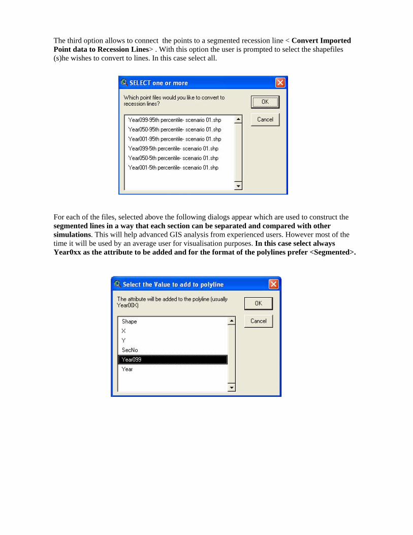
The third option allows to connect the points to a segmented recession line < Convert Imported Point data to Recession Lines> . With this option the user is prompted to select the shapefiles (s)he wishes to convert to lines. In this case select all.

For each of the files, selected above the following dialogs appear which are used to construct the segmented lines in a way that each section can be separated and compared with other simulations. This will help advanced GIS analysis from experienced users. However most of the time it will be used by an average user for visualisation purposes. In this case select always Year0xx as the attribute to be added and for the format of the polylines prefer <Segmented>.

The results of this procedure is shown in the next figure. Again the name of the file is showing what the file is about.

And the last option to segmented polygon areas of land lost <Build Risk Zones (as polygons)>. The polygons are segmented at the section divisions. An example of the results is shown in the following figure. The navy blue area is the cliff top recession at the 5th percentile of the pdf (from the current cliff positions) in 50 years if scenario 01 is applied. The green area is the is the cliff top recession at the 95th percentile of the pdf which covers the navy blue area as well. The visible part of the 95th percentile cliff top recession is the the zone between 5th -95th percentiles, in other words the area where the cliff top is likely to be in 50 years according to the model and the scenario 01. The fact that the risk zone is segmented allows for the calculation of the erosion impact in each section.

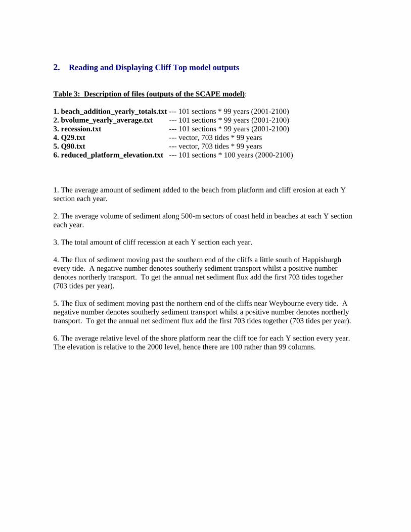
2. Reading and Displaying Cliff Top model outputs Table 3: Description of files (outputs of the SCAPE model): 1. beach_addition_yearly_totals.txt --- 101 sections * 99 years (2001-2100) 2. bvolume_yearly_average.txt --- 101 sections * 99 years (2001-2100) 3. recession.txt --- 101 sections * 99 years (2001-2100) 4. Q29.txt --- vector, 703 tides * 99 years 5. Q90.txt --- vector, 703 tides * 99 years 6. reduced_platform_elevation.txt --- 101 sections * 100 years (2000-2100) 1. The average amount of sediment added to the beach from platform and cliff erosion at each Y section each year. 2. The average volume of sediment along 500-m sectors of coast held in beaches at each Y section each year. 3. The total amount of cliff recession at each Y section each year. 4. The flux of sediment moving past the southern end of the cliffs a little south of Happisburgh every tide. A negative number denotes southerly sediment transport whilst a positive number denotes northerly transport. To get the annual net sediment flux add the first 703 tides together (703 tides per year). 5. The flux of sediment moving past the northern end of the cliffs near Weybourne every tide. A negative number denotes southerly sediment transport whilst a positive number denotes northerly transport. To get the annual net sediment flux add the first 703 tides together (703 tides per year). 6. The average relative level of the shore platform near the cliff toe for each Y section every year. The elevation is relative to the 2000 level, hence there are 100 rather than 99 columns.

The third option of the main dialogue (figure 2) enables the user to read the outputs of the SCAPE model in the format they were originally generated and converts them into an AV friendly format. The following dialog appears upon the selection of this option.

An example of the use of this dialogue is given below: a. Click on the first button. A Dialogue appears and the user is prompted to locate the executable file (readmodeloW.exe). This should be in the directory created by the zip file you were given. b. As the readmodeloW program runs it prompts the user to enter the file with the model outputs (e.g. modelout.txt). This file should be in the same directory as the readmodelow.exe file. c. Enter the number of sections (eg 100) d. Enter the number of simulations: 100 (for the modelout.txt file). e. Enter the name of the output file (e.g. out.txt) An AV friendly model output has been created (out.txt). This file can be used as input to the second option of the dialog above in order to input the data as Arcview Tables. For example: Click on the second button (pin icon). Select e.g. out.txt and a table named "Recession Distance" will be created in ArcView. If you are running the script for a second time then you will be prompted whether you wish to retain or replace this table. The fourth option of the main dialogue (figure 2), is followed with the dialog as shown in the figure below and works in similar way as the cliff tops.

3. Estimate Impacts of Cliff Erosion to Coastal Areas 4. Finally the last option <Estimate Impacts of Cliff Erosion to Coastal Areas> allows the user to estimate land losses due to the simulated cliff erosion. If Land Use and Infrastructure data are available then the types of Land Uses and and the number if Infrastructure (e.g. Buildings) can be estimated. The following figure* shows the available options to the user.

In this step the user can build polygons in order to assess the impact of erosion to land uses. The north and south sides of the polygons are the section (transect) lines. The east side can be the segment between two points showing the current position of the cliff (e.g. cliff toe or top at year 2000) and the west side is the segment showing the recessed position as predicted using the SCAPE GIS model. In this way the user can build polygons for every section to estimate land loss between the position in the “current” year and a predicted position (e.g. year 37, 100 etc).

The east side (start) can also be a segment representing the position of cliffs at a specific year/simulation. For example the user might need to build a polygon for a section between the year (simulation) 10 and 25, to see what land lost during this period. In both cases the user is able to select multiple years (simulations) and build multiple polygon files. If the user chooses to create polygons not starting at the current positions then a point file with the start year must exist to specify the initial coordinates. Polygon files are saved as <Pol_year0xx.shp>, where 0xx is the year number. For Cliff top files use the polygons created in the Cliff Top dialogues and proceed to the following option to estimate land losses. <Show Area Lost due to Erosion (per Land Cover Type)> Using this option in the dialogue the user is able to create a cross tabulation of Section-Polygons (created in the previous step) and Land Use data (Corine in this case – File: Clip_lc2000.shp) Corine data should already be loaded in <CliffScapeLink> View. Next the user is prompted to input the name of the Corine data file. Select Clip_lc2000.shp (this is to determine the extent of a temporary grid – no need to know this…) In the dialogue that follows the user should select the Row and the Column theme/field in order to cross tabulate the data.

As Row theme select: Pol_year0xx.shp (a polygon-section file) As Row Field select: SecNo (section number field) As Column Theme select: Clip_lc2000.shp (Corine data) As Column Field select: Class (the field with the class names or codes) (the order of the themes can change depending on the type of table desired)

A table named “Land Types Lost per Section” has been created with row and columns sums calculated. This table can be exported to Excel (File> Export) for further descriptive processing if necessary. 5. General Tools for SCAPE model Pressing the Tools button the following dialogue appears.

The first two tools are very simple and refer to the construction of a Baseline. <Find new Coords to shift Baseline>, <Create New Baseline and Sections>. The second used the following form.

The next option <Create Intersection points of shorelines and Section Lines> is using an existed script (view.polyint2pnt from ESRI), modified for the needs of the SCAPEGIS extension, to create intersection points between sections and coastlines. When the files with the intersection points are created the user can use the <Calculate Distance between two Lines with IDs (0,1)> option to calculate the distance between the coastlines at the points that intersect

the section lines used by the model. In order for the routine to work properly the Coastlines file must have two lines coded as 0 and 1 respectively in the ID field. The last pair of options can help the user identify how many elements (e.g. buildings) have been lost due to erosion. The polygon files created earlier should be used for this task. <Select Polygons of Specific Sections> with this option the user can specify a number of sections and examine the loss of elements (e.g. buildings) for these particular sections. If not used it would be assumed that all sections are selected. <Select Features using polygons of specific sections> First the user is prompted to select the feature (elements) file. Select: Buildings.shp (this file must already be loaded to the CliffScapeLink view. In the dialogue that appears next, Select Features of active theme (the theme you just selected above e.g. Buildings.shp) that <Intersect> the selected features (selected sections with the previous option) of : <Select a polygon-section file. E.g. Pol_year050.shp)> And then select New Set to create a new set of elements using the above criteria in order to get the number of elements (buildings) lost. Note: The software asks the user to input most of the variables involved. By doing so, it enables the user to change the original data and the filenames. This allows for great flexibility and other models can be used if they are following the data format specified above! Contact: Sotiris Koukoulas (skouk@geo.aegean.gr) * This dialogue includes the "PT_LN_PL.AVE" script which was originally written by Nielsen D., 1998 and was modified here by permission. 'PT_LN_PL.AVE 'Original author Daniel Nielsen August 31, 1998 'Modified by Dan Patterson Jan 28, 1999 'Modified by Sotiris Koukoulas Aug 2003 References: Brown I., S. Jude, S. Koukoulas, R. Nicholls, M. Dickson, M. Walkden, and A. Jones, (2004) Dynamic Simulation and Visualisation of Coastal Erosion: Past, Present and Future, GISRUK04, University of East Anglia, Norwich, 28-30 April 2004. Walkden, M. J. & Hall, J. W. (2002) A model of soft cliff and platform erosion. Proceedings of the 28th International Conference on Coastal Engineering 2002, Volume 3 (pp3333-3345).

The inter-disciplinary Tyndall Centre for Climate Change Research undertakes integrated research into the long-term consequences of climate change for society and into the development of sustainable responses that governments, business-leaders and decision-makers can evaluate and implement. Achieving these objectives brings together UK climate scientists, social scientists, engineers and economists in a unique collaborative research effort.

Research at the Tyndall Centre is organised into four research themes that collectively contribute to all aspects of the climate change issue: Integrating Frameworks; Decarbonising Modern Societies; Adapting to Climate Change; and Sustaining the Coastal Zone. All thematic fields address a clear problem posed to society by climate change, and will generate results to guide the strategic development of climate change mitigation and adaptation policies at local, national and global scales.

The Tyndall Centre is named after the 19th century UK scientist John Tyndall, who was the first to prove the Earth’s natural greenhouse effect and suggested that slight changes in atmospheric composition could bring about climate variations. In addition, he was committed to improving the quality of science education and knowledge.

The Tyndall Centre is a partnership of the following institutions: University of East Anglia University of Manchester Southampton Oceanography Centre University of Southampton University of Cambridge Centre for Ecology and Hydrology SPRU – Science and Technology Policy Research (University of Sussex) Institute for Transport Studies (University of Leeds) Complex Systems Management Centre (Cranfield University) Energy Research Unit (CLRC Rutherford Appleton Laboratory)

The Centre is core funded by the following organisations: Natural Environmental Research Council (NERC) Economic and Social Research Council (ESRC) Engineering and Physical Sciences Research Council (EPSRC) UK Government Department of Trade and Industry (DTI) For more information, visit the Tyndall Centre Web site (www.tyndall.ac.uk) or contact:

Communications Manager Tyndall Centre for Climate Change Research University of East Anglia, Norwich NR4 7TJ, UK Phone: +44 (0) 1603 59 3906; Fax: +44 (0) 1603 59 3901 Email: tyndall@uea.ac.uk

Recent Tyndall Centre Technical Reports Tyndall Centre Technical Reports are available online at http://www.tyndall.ac.uk/publications/tech_reports/tech_reports.shtml

Pearson, S., Rees, J., Poulton, C., Dickson, M., Walkden, M., Hall, J., Nicholls, R., Mokrech, M., Koukoulas, S. and Spencer, T. (2005) Towards an integrated coastal sediment dynamics and shoreline response simulator, Tyndall Centre Technical Report 38

Sorrell, S. (2005) The contribution of energy service contracting to a low carbon economy, Tyndall Centre Technical Report 37

Tratalos, J. A., Gill, J. A., Jones, A., Showler, D., Bateman, A., Watkinson, A., Sugden, R., and Sutherland, W. (2005) Interactions between tourism, breeding birds and climate change across a regional scale, Tyndall Centre Technical Report 36

Thomas, D., Osbahr, H., Twyman, C., Adger, W. N. and Hewitson, B., (2005) ADAPTIVE: Adaptations to climate change amongst natural resource-dependant societies in the developing world: across the Southern African climate gradient, Tyndall Centre Technical Report 35

Arnell, N. W., Tompkins, E. L., Adger, W. N. and Delany, K. (2005) Vulnerability to abrupt climate change in Europe, Tyndall Centre Technical Report 34

Shackley, S. and Anderson, K. et al. (2005) Decarbonising the UK: Energy for a climate conscious future, Tyndall Technical Report 33

Halliday, J., Ruddell, A., Powell, J. and Peters, M. (2005) Fuel cells: Providing heat and power in the urban environment, Tyndall Centre Technical Report 32

Haxeltine, A., Turnpenny, J., O’Riordan, T., and Warren, R (2005) The creation of a pilot phase Interactive Integrated Assessment Process for managing climate futures, Tyndall Centre Technical Report 31

Nedic, D. P., Shakoor, A. A., Strbac, G., Black, M., Watson, J., and Mitchell, C. (2005) Security assessment of futures electricity scenarios, Tyndall Centre Technical Report 30

Shepherd, J., Challenor, P., Marsh, B., Williamson, M., Yool, W., Lenton, T., Huntingford, C., Ridgwell, A and Raper, S. (2005) Planning and Prototyping a Climate Module for the Tyndall Integrated Assessment Model, Tyndall Centre Technical Report 29

Lorenzoni, I., Lowe, T. and Pidgeon, N. (2005) A strategic assessment of scientific and behavioural perspectives on ‘dangerous’ climate change, Tyndall Centre Technical Report 28

Boardman, B., Killip, G., Darby S. and Sinden, G, (2005) Lower Carbon Futures: the 40% House Project, Tyndall Centre Technical Report 27

Dearing, J.A., Plater, A.J., Richmond, N., Prandle, D. and Wolf , J. (2005) Towards a high resolution cellular model for coastal simulation (CEMCOS), Tyndall Centre Technical Report 26

Timms, P., Kelly, C., and Hodgson, F., (2005) World transport scenarios project, Tyndall Centre Technical Report 25

Brown, K., Few, R., Tompkins, E. L., Tsimplis, M. and Sortti, (2005) Responding to climate change: inclusive and integrated coastal analysis, Tyndall Centre Technical Report 24

Anderson, D., Barker, T., Ekins, P., Green, K., Köhler, J., Warren, R., Agnolucci, P., Dewick, P., Foxon, T., Pan, H. and Winne, S. (2005) ETech+: Technology policy and technical change, a dynamic global and UK approach, Tyndall Centre Technical Report 23

Abu-Sharkh, S., Li, R., Markvart, T., Ross, N., Wilson, P., Yao, R., Steemers, K., Kohler, J. and Arnold, R. (2005) Microgrids: distributed on-site generation, Tyndall Centre Technical Report 22

Shepherd, D., Jickells, T., Andrews, J., Cave, R., Ledoux, L, Turner, R., Watkinson, A., Aldridge, J. Malcolm, S, Parker, R., Young, E., Nedwell, D. (2005) Integrated modelling of an estuarine environment: an assessment of managed realignment options, Tyndall Centre Technical Report 21

Dlugolecki, A. and Mansley, M. (2005) Asset management and climate change, Tyndall Centre Technical Report 20

Shackley, S., Bray, D. and Bleda, M., (2005) Developing discourse coalitions to incorporate stakeholder perceptions and responses within the Tyndall Integrated Assessment, Tyndall Centre Technical Report 19

Dutton, A. G., Bristow, A. L., Page, M. W., Kelly, C. E., Watson, J. and Tetteh, A. (2005) The Hydrogen energy economy: its long term role in greenhouse gas reduction, Tyndall Centre Technical Report 18

Few, R. (2005) Health and flood risk: A strategic assessment of adaptation processes and policies, Tyndall Centre Technical Report 17

Brown, K., Boyd, E., Corbera-Elizalde, E., Adger, W. N. and Shackley, S (2004) How do CDM projects contribute to sustainable development? Tyndall Centre Technical Report 16

Levermore, G, Chow, D., Jones, P. and Lister, D. (2004) Accuracy of modelled extremes of temperature and climate change and its implications for the built environment in the UK, Tyndall Centre Technical Report 14

Jenkins, N., Strbac G. and Watson J. (2004) Connecting new and renewable energy sources to the UK electricity system, Tyndall Centre Technical Report 13

Palutikof, J. and Hanson, C. (2004) Integrated assessment of the potential for change in storm activity over Europe: Implications for insurance and forestry, Tyndall Centre Technical Report 12

Berkhout, F., Hertin, J., and Arnell, N. (2004) Business and Climate Change: Measuring and Enhancing Adaptive Capacity, Tyndall Centre Technical Report 11

Tsimplis, S. et al (2004) Towards a vulnerability assessment for the UK coastline, Tyndall Centre Technical Report 10

Gill, J., Watkinson, A. and Côté, I (2004). Linking sea level rise, coastal biodiversity and economic activity in Caribbean island states: towards the development of a coastal island simulator, Tyndall Centre Technical Report 9

Skinner, I., Fergusson, M., Kröger, K., Kelly, C. and Bristow, A. (2004) Critical Issues in Decarbonising Transport, Tyndall Centre Technical Report 8

Adger W. N., Brooks, N., Kelly, M., Bentham, S. and Eriksen, S. (2004) New indicators of vulnerability and adaptive capacity, Tyndall Centre Technical Report 7

Macmillan, S. and Köhler, J.H., (2004) Modelling energy use in the global building stock: a pilot survey to identify available data, Tyndall Centre Technical Report 6

Steemers, K. (2003) Establishing research directions in sustainable building design, Tyndall Centre Technical Report 5

Goodess, C.M. Osborn, T. J. and Hulme, M. (2003) The identification and evaluation of suitable scenario development methods for the estimation of future probabilities of extreme weather events, Tyndall Centre Technical Report 4

Köhler, J.H. (2002). Modelling technological change, Tyndall Centre Technical Report 3

Gough, C., Shackley, S., Cannell, M.G.R. (2002). Evaluating the options for carbon sequestration, Tyndall Centre Technical Report 2

Warren, R. (2002). A blueprint for integrated assessment of climate change, Tyndall Centre Technical Report 1