Embed Size (px)
Citation preview
BAMBERGER BEITRÄGE ZURWIRTSCHAFTSINFORMATIK UND ANGEWANDTEN INFORMATIK
ISSN 0937-3349
Nr. 77/2008
Towards Constructive DescriptionLogics for Abstraction and Refinement
Stephan Scheele and Michael Mendler
FAKULTÄT FÜRWIRTSCHAFTSINFORMATIK UND ANGEWANDTE INFORMATIK
OTTO-FRIEDRICH-UNIVERSITÄT BAMBERG
Towards Constructive Description Logics
for Abstraction and Refinement ∗ †
Michael Mendler, Stephan Scheele
Faculty of Information Systems and Applied Computer Sciences
The Otto-Friedrich-University of Bamberg, Germany
{michael.mendler,stephan.scheele}@uni-bamberg.de
September 2008
Abstract
This work explores some aspects of a new and natural semantical dimension
that can be accommodated within the syntax of description logics which opens
up when passing from the classical truth-value interpretation to a constructive
interpretation. We argue that such a strengthened interpretation is essential to
represent applications with partial information adequately and to achieve consis-
tency under abstraction as well as robustness under refinement. We introduce a
constructive version of ALC, called cALC, for which we give a sound and com-
plete Hilbert axiomatisation and a Gentzen tableau calculus showing finite model
property and decidability.
1 Introduction
The successes of description logics (DLs) in the many domains of semantic information
processing is based on their flexibility to strike a carefully crafted trade-off between
expressiveness and implementation efficiency. DLs have their origin in knowledge rep-
resentation formalisms. They aim to encapsulate semantical complexity in compact
notation which is domain-specific rather than general purpose. This leverages syntax
to make the handling of logical specifications both by humans as well as reasoning
engines run in a much higher gear (‘application-level’) compared to, say, plain vanilla
∗An extended abstract of this work has been presented at the 21th International Workshop on De-scription Logics (DL2008).
†This word is funded by the German Research Council (DFG) as part of the project SPACMODLgrant No. ME 1427/4-1.
1
M. Mendler, S. Scheele Towards Constructive DL for Abstraction and Refinement
first-order logic, in which all quantification structure is made explicit (‘representation-
level’).
Technically, DLs are related to multi-dimensional generalisations of modal logic [15, 1]
and as such they are essentially guarded fragments of first-order logic. These frag-
ments have turned out to be a breeding-ground of very well-behaved classes of logic
formalisms. This work explores some aspects of yet another semantical dimension that
can be accommodated within the syntax of DL which opens up when passing from the
classical truth-value interpretation to a constructive interpretation of DL. We will ar-
gue that such a refined interpretation is essential to represent applications with partial
information adequately and to achieve both consistency under abstraction as well as
robustness under refinement.
1.1 When Constructiveness Matters
Knowledge representation based on description logics can be used to capture the mean-
ing of natural language statements about specific world domains (ontologies). Often,
however, such knowledge is dynamic and incomplete. Entities that make up the domain
may not be fixed and tangible but abstractions of real individuals whose properties are
changing and defined only up to construction. Natural language concepts rarely have
a static interpretation but are subject to negotiation or context and thus require a
constructive approach which is robust under refinement.
An application area where this aspect is particularly prominent and which motivates
the work described here, is auditing. The digital auditing of business mass data expe-
riences a huge increase in importance recently. Audit executives, fraud examiners and
compliance professionals are pressured on all fronts to shorten audit cycles and to in-
crease audit efficiency and quality. In particular, the efficient verification of enterprise
processes is of big interest since the audit concern is getting more critical with new
regulations like SOX1, IFRS2 and also to respond accurately to managing risks in our
competitive world.
1Sarbanes-Oxley Act, US law of 2002 on business reporting in reaction to Enron and WorldComscandals.
2International Financial Reporting Standard.
WIAI, University of Bamberg 2 Technical Report 77(2008)
M. Mendler, S. Scheele Towards Constructive DL for Abstraction and Refinement
Audit statements about the validity of accounting data, absence of fraud or conformance
to financial process standards must constructively take account of many dimensions of
abstraction and refinement.
• First, the producers of audit data usually are ongoing business processes which
the audit data can only cover a limited snapshot of. E.g., a requirement such as
“each delivery order must have an associated invoice” must take into account that
for some delivery order the invoice is still “in the process” and only available after
refinement of the audit data.
• Second, a role like the ‘legally responsible signatory’ may not be fully definable
once and for all but depend on the legal context. Some aspects may even delib-
erately be left open subject to negotiations and only refined as the auditing case
progresses.
• Third, entities may be abstractions of physical individuals: The notion of the
‘CEO of company X’ in an audit statement is a virtual rather than concrete
person who may be replaced perhaps while auditing is ongoing. The CEO which
appears atomic at some level of abstraction really is a concept at a lower level
where personal liability issues come in or where executive action needs to be
taken.
• Forth, auditing is typically faced with vast amounts of business data. For effi-
ciency reasons, manageable digests of the data need to be created. Such data
compression may ignore purportedly irrelevant attributes of entities or scan only
a subset of entities associated with a given concept. Auditing, thus, is not ex-
act but approximated. If the quick check indicates potential irregularities then a
constructive refinement of the abstracted entities and concepts must be possible
to confirm or reject the case constructively. For instance, a Benford test [6] may
show an abnormal distribution of digits in the sales slips of a retail chain. How-
ever, when taking into account the abstracted “irrelevant” data it may turn out
that the deviation can be explained by a special promotion offer. The auditing
domain demands a constructive concept of truth to take care of the potential
incompleteness of knowledge.
Auditing is a prime example of a class of application domains which require the ability
to express partiality and incomplete information beyond the standard open world as-
WIAI, University of Bamberg 3 Technical Report 77(2008)
M. Mendler, S. Scheele Towards Constructive DL for Abstraction and Refinement
sumption (OWA). Because the semantical meaning is context-dependent and possibly
involves many levels of explication there must be a constructive notion of undefinedness
which permits that concepts evolve. Classical OWA assumes that each concept is static
and at the outset either includes a given entity or not. However, either option may be
incorrect, if the entity or the concept is not fully defined until a later stage where lower
levels of detail become available. The critical issue is that there will be entities which
have the same abstract properties (such as sharing the same fillers and concepts) but
still are distinct individuals at some level so that identifying them at the outset would
be inconsistent.
But if OWA is not enough, how can reasoning be both correct under abstraction and
sustainable under refinement? Logic offers a well-known suggestion to solve this puzzle
which is to replace the traditional binary truth interpretation by a constructive notion
of truth. Proof-theoretically, constructive logic is compatible with the idea of positive
evidence and realisability [25]. It does not infer the presence of entities from the absence
of others but insists on the existence of computational witnesses. Model-theoretically,
constructive logic admits of an interpretation based on stages of information [27] so
that truth is persistent under refinement3.
1.2 Related Work
The role of intuitionistic Kripke models for knowledge representation based on partial
descriptions has been highlighted in [9]. The general benefits of the Curry-Howard Iso-
morphism (proofs-as-computations) in DL have been argued in [11, 8]. In our context,
more concretely, we envisage that the computational interpretation of TBox deductions
as λ-terms yields verified audit tactics and that constructive ABox tableau algorithms
provide engines to drive interactive games between auditee (proponent) and auditor
(opponent). A third potential benefit arises from the use of DLs as a programming type
system (see e.g., [19]) which naturally requires a constructive setting. Constructive DL
concepts may not only specify the semantics of data streams in audit component inter-
faces but also resource requirements. This can be exploited to satisfy higher demands
on robustness and efficiency in the semantic processing of mass data.
3One might say that classical DL is based on a static open world assumption (SOWA) while con-structive DL supports an evolving open world assumption (EOWA).
WIAI, University of Bamberg 4 Technical Report 77(2008)
M. Mendler, S. Scheele Towards Constructive DL for Abstraction and Refinement
In this work we discuss some of the model-theoretic aspects of the constructive inter-
pretation of DLs, in contrast to [8] which is proof-theoretic and addresses the extraction
of information terms.
The work of [9] presents an intuitionistic epistemic logic based on several refinement
relations coding multiple (partial) points of view. Here we only consider one dimen-
sion of refinement reflecting a two-player scenario (e.g., auditor and auditee) but in a
more general sense than [9]. Our refinement ordering � may have cycles and fallible
descriptions. Such descriptive “oscillations” and “deadlocks” are intrinsic to real-world
abstractions (see examples below). The notion of a simulation relation such as in [10]
for semi-structured data (BDFS) can also be thought of as a refinement relation. How-
ever, it is an external meta-level concept on models and cannot be iterated. In the
description logic cALC proposed here refinement is internal and transitive to represent
nested levels of concretisations inside a single model.
It is important to point out that the semantic dimension along which refinement takes
place is implicit in cALC and not coded in the syntax. This accommodates many
different notions of context generically in the language of the basic description logic ALC
[4]. The context-dependency is built into the notion of truth rather than the terminology
like in other work on special cases of context such as temporal DL [2, 7, 3]. cALC is
meant for applications where we must be robust for several implicit notions of context-
dependency but do not need to reason explicitly about some specific refinement.
Our work is to be distinguished also from many-valued DL (see e.g., [20, 17]) which is
finitely valued while cALC is infinitely valued and from fuzzy DL (see e.g., [24, 12, 16])
which use a quantitative notion of approximate truth whereas cALC still adheres to a
crisp deductive approach. Even though the envisaged application domain of auditing
may use statistical analyses, at the end of the day we must cross the t’s and dot the i’s
and be able to name the evidence.
1.3 Overview & Summary of Results
Section 2 introduces the syntax and semantics of cALC and presents several examples
for applications where constructivity is needed. Section 3 gives a sound and complete
Hilbert axiomatisation and a Gentzen-tableau deduction system for cALC, showing
WIAI, University of Bamberg 5 Technical Report 77(2008)
M. Mendler, S. Scheele Towards Constructive DL for Abstraction and Refinement
finite model property and decidability. The computational aspects are covered by fol-
lowing the Curry-Howard-Isomorphism and presented in a detailed example. Finally
the complexity of reasoning in cALC is addressed. Section 4 discusses the semantical
dimensions between cALC and ALC and to what extent cALC is a constructive weak-
ening of classical ALC. Finally, section 5 concludes our results and gives insights into
future work.
2 Syntax and Semantics of cALC
Concept descriptions in cALC are based on sets of role names NR and concept names
NC and are formed as follows, where A ∈ NC and R ∈ NR:
C, D → A | ⊤ | ⊥ | ¬C | C ⊓ D | C ⊔ D | C ⊑ D | ∃R.C | ∀R.C.
This syntax is more general than standard ALC in that it includes subsumption ⊑ as
a concept-forming operator. The TBox statement C ⊑ D meaning that ‘D subsumes
C’ is expressed as the concept identity C ⊑ D = ⊤. In classical ALC one could use the
equation ¬C ⊔D = ⊤ to do that, essentially reducing subsumption to ¬ and ⊔. This is
no longer possible in constructive logic where these operators are independent. Being
a first class operator, subsumption can be nested arbitrarily as in ((D ⊑ C) ⊑ B) ⊑ A.
The full power of such “higher–order” subsumptions may not be needed in practice but
will allow us to axiomatise the full theory of cALC conveniently in the form of a Hilbert
calculus. Like in ALC the universal concept ⊤ is redundant and codable as ¬⊥. Also,
⊥ and ¬ can represent each other, e.g. ⊥ = A⊓¬A and ¬C = C ⊑ ⊥. Otherwise, the
operators are independent.
Constructive interpretations I of concept descriptions extend the classical models for
ALC by a pre-ordering �I for expressing refinement between individuals and by a
notion of fallible entities ⊥I for interpreting contradiction.
Following the standard Kripke semantics of intuitionistic logic [27], entities in construc-
tive DL are not atomic individuals but have internal structure which in general is only
partially determined and thus subject to refinement. Let relation a � a′ on entities
denote that a′ is more precisely determined than a, that a′ refines a or that a abstracts
a′. The relation � models a potential increase of information or refinement of context
WIAI, University of Bamberg 6 Technical Report 77(2008)
M. Mendler, S. Scheele Towards Constructive DL for Abstraction and Refinement
associated with the process of pinning down entities as real individuals. This includes
the possibility that both a � b and b � a, i.e., a and b have the same information
content and thus are formally indistinguishable, yet still distinct a 6= b because of some
lower-level properties. Now, if a concept C is to be robust under refinement then a:C
and a � a′ must imply a′:C. This is achieved by the following definition:
Definition 1. A constructive interpretation or constructive model of cALC is a struc-
ture I = (∆I ,�I ,⊥I , ·I) consisting of
• a non-empty set ∆I of entities, the universe of discourse in which each entity
represents a partially defined, or abstract individual;
• a refinement pre-ordering �I on ∆I , i.e., a reflexive and transitive relation;
• a subset ⊥I ⊆ ∆I of fallible entities closed under refinement, i.e., x ∈ ⊥I and
x �I y implies y ∈ ⊥I , for every fallible entity x exists a fallible filler z, i.e.,
xR z & z ∈ ⊥I and all filler of a fallible entity x are fallible, i.e. ∀z. xR z ⇒ z ∈
⊥I ;
• finally an interpretation function ·I mapping each role name R ∈ NR to a binary
relation RI ⊆ ∆I ×∆I and each atomic concept A ∈ NC to a set ⊥I ⊆ AI ⊆ ∆I
which is closed under refinement, i.e., x ∈ AI and x �I y implies y ∈ AI .
The interpretation I is lifted from atomic ⊥, A to arbitrary concepts, where ∆Ic =df
∆I \ ⊥I is the set of non-fallible elements in I:
⊤I =df ∆I
(¬C)I =df {x | ∀y ∈ ∆Ic . x �I y ⇒ y 6∈ CI}
(C ⊓ D)I =df CI ∩ DI
(C ⊔ D)I =df CI ∪ DI
(C ⊑ D)I =df {x | ∀y ∈ ∆I . (x �I y & y ∈ CI) ⇒ y ∈ DI}
(∃R.C)I =df {x | ∀y ∈ ∆I . x �I y ⇒ ∃z ∈ ∆I . (y, z) ∈ RI & z ∈ CI}
(∀R.C)I =df {x | ∀y ∈ ∆I . x �I y ⇒ ∀z ∈ ∆I . (y, z) ∈ RI ⇒ z ∈ CI}.
Entities in ∆I are partial descriptions representing incomplete information about in-
dividuals. Fallible elements b ∈ ⊥I may be thought of as over-constrained tokens of
information, self-contradictory objects of evidence or undefined computations. E.g.,
WIAI, University of Bamberg 7 Technical Report 77(2008)
M. Mendler, S. Scheele Towards Constructive DL for Abstraction and Refinement
they may be used to model the situation in which computing a role-filler for an ab-
stract individual a fails, i.e., ∀b. R(a, b) ⇒ b ∈ ⊥I , yet when a is refined to a′ then a
non-fallible role-filler b′ ∈ ∆Ic exists with R(a′, b′) (see Example 3 below).
Because of the abstraction fuzziness embodied by �I and ⊥I the elements of ∆I are
abstract individuals or entities rather than concrete or atomic individuals (which are a
fiction anyway, constructively speaking).
Each entity implicitly subsumes all its refinements and truth is inherited. Specifically,
one can show that x ∈ CI and x �I y implies y ∈ CI for all concepts C. Fallible entities
are information-wise maximal elements and therefore included in every concept, i.e.,
⊥I ⊆ CI for all C.
Lemma 1. For all concepts C it holds that ∀a ∈ ∆I .a ∈ ⊥I ⇒ a ∈ CI .
Proof. The proof is by induction on the structure of C. The detailed proof is given in
the appendix.
The purpose of the present work is to show that the non-standard interpretation of
Def. 1 induces a well-behaved logic, called cALC, which uses the same syntax but is
more expressive than classical ALC and still admits standard TBox and ABox tableau
reasoning. Before we continue expounding the theory let us look at some examples.
Example 1. Every classical interpretation I of ALC (see e.g., [4]) induces a trivial
model according to Def. 1 with the discrete refinement relation �I , i.e., the identity
relation x �I y iff x = y and the empty set ⊥I = ∅ of fallible entities. These validate
the formulas C ⊔ ¬C = ⊤, ∃R.⊥ = ⊥ and ∃R.(C ⊔ D) = ∃R.C ⊔ ∃R.D. These three
axioms essentially characterise classical models (see Sec. 4).
Example 2. Let a = (c, d1) and b = (c, d2) be two entries in a (relational) database
that share the same first attribute but are distinguished in the second. If the attributes
are referenced by roles $1 and $2 then the situation could be specified, in ABox syntax,
by a $1 c, a $2 d1, b $1 c, b $2 d2. Now let us abstract from the second attributes and
consider the pairs as partially defined entities a♯ = (c, ?) and b♯ = (c, ?), respectively,
say in an attempt to compress information. Ignoring d1, d2 means that a♯ and b♯ carry
the same information and thus can no longer be distinguished. Since the pre-order �
measures the information content the entities a♯ and b♯ are mutually reachable via � and
refine each other, i.e. a♯ � b♯ and b♯ � a♯. This cyclic refinement relationship between
WIAI, University of Bamberg 8 Technical Report 77(2008)
M. Mendler, S. Scheele Towards Constructive DL for Abstraction and Refinement
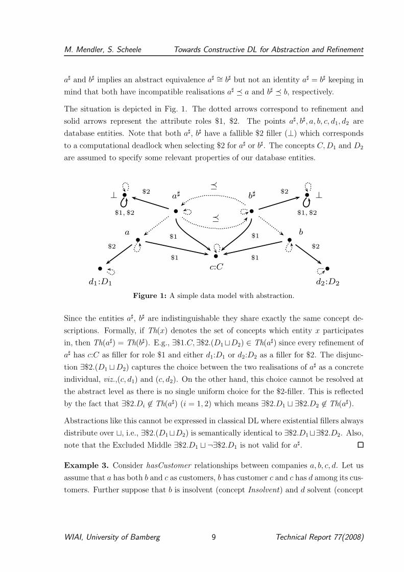
a♯ and b♯ implies an abstract equivalence a♯ ∼= b♯ but not an identity a♯ = b♯ keeping in
mind that both have incompatible realisations a♯ � a and b♯ � b, respectively.
The situation is depicted in Fig. 1. The dotted arrows correspond to refinement and
solid arrows represent the attribute roles $1, $2. The points a♯, b♯, a, b, c, d1, d2 are
database entities. Note that both a♯, b♯ have a fallible $2 filler (⊥) which corresponds
to a computational deadlock when selecting $2 for a♯ or b♯. The concepts C, D1 and D2
are assumed to specify some relevant properties of our database entities.
b b
b b
b b
a♯
b
b b⊥ ⊥
ba
b♯
c:C
d1:D1 d2:D2
�
�$2 $2
$1 $1
$1 $1
$2$2
$1, $2 $1, $2
Figure 1: A simple data model with abstraction.
Since the entities a♯, b♯ are indistinguishable they share exactly the same concept de-
scriptions. Formally, if Th(x) denotes the set of concepts which entity x participates
in, then Th(a♯) = Th(b♯). E.g., ∃$1.C, ∃$2.(D1⊔D2) ∈ Th(a♯) since every refinement of
a♯ has c:C as filler for role $1 and either d1:D1 or d2:D2 as a filler for $2. The disjunc-
tion ∃$2.(D1 ⊔D2) captures the choice between the two realisations of a♯ as a concrete
individual, viz.,(c, d1) and (c, d2). On the other hand, this choice cannot be resolved at
the abstract level as there is no single uniform choice for the $2-filler. This is reflected
by the fact that ∃$2.Di 6∈ Th(a♯) (i = 1, 2) which means ∃$2.D1 ⊔ ∃$2.D2 6∈ Th(a♯).
Abstractions like this cannot be expressed in classical DL where existential fillers always
distribute over ⊔, i.e., ∃$2.(D1⊔D2) is semantically identical to ∃$2.D1⊔∃$2.D2. Also,
note that the Excluded Middle ∃$2.D1 ⊔ ¬∃$2.D1 is not valid for a♯.
Example 3. Consider hasCustomer relationships between companies a, b, c, d. Let us
assume that a has both b and c as customers, b has customer c and c has d among its cus-
tomers. Further suppose that b is insolvent (concept Insolvent) and d solvent (concept
WIAI, University of Bamberg 9 Technical Report 77(2008)
M. Mendler, S. Scheele Towards Constructive DL for Abstraction and Refinement
¬Insolvent). Regarding possible insolvency of c nothing is known. In classical OWA
we have c:(Insolvent ⊔¬Insolvent) regardless of c. This implies that a is an instance of
the concept description CW = ∃hasCustomer .(Insolvent ⊓ ∃hasCustomer .¬Insolvent)
specifying credit-worthy companies with an insolvent customer who in turn can rely on
at least one solvent customer. In the first case c:Insolvent this customer of a is c, in
case c:¬Insolvent it is b. In a static world the filling customer would be unknown but
fixed. However, the case analysis on c is invalid if the model arises by abstraction from
a concrete taxonomy where insolvency is a context-dependent defect.
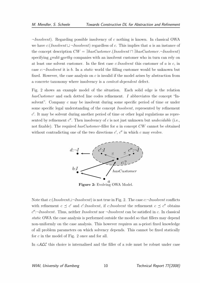
Fig. 2 shows an example model of the situation. Each solid edge is the relation
hasCustomer and each dotted line codes refinement. I abbreviates the concept “In-
solvent”. Company c may be insolvent during some specific period of time or under
some specific legal understanding of the concept Insolvent, represented by refinement
c′. It may be solvent during another period of time or other legal regulations as repre-
sented by refinement c′′. Then insolvency of c is not just unknown but undecidable (i.e.,
not fixable). The required hasCustomer-filler for a in concept CW cannot be obtained
without contradicting one of the two directions c′, c′′ in which c may evolve.
b
b
b
b bb
a
c:?
c′:I c′′:¬I
b:I
d:¬I
hasCustomer
� �
Figure 2: Evolving OWA Model.
Note that c:(Insolvent⊔¬Insolvent) is not true in Fig. 2. The case c:¬Insolvent conflicts
with refinement c � c′ and c′:Insolvent, if c:Insolvent the refinement c � c′′ obtains
c′′:¬Insolvent . Thus, neither Insolvent nor ¬Insolvent can be satisfied in c. In classical
static OWA the case analysis is performed outside the model so that fillers may depend
non-uniformly on the case analysis. This however requires an a-priori fixed knowledge
of all problem parameters on which solvency depends. This cannot be fixed statically
for c in the model of Fig. 2 once and for all.
In cALC this choice is internalised and the filler of a role must be robust under case
WIAI, University of Bamberg 10 Technical Report 77(2008)
M. Mendler, S. Scheele Towards Constructive DL for Abstraction and Refinement
analysis. Thus, a:CW is invalid under Evolving OWA because the ∃-filler is not realis-
able by a single nameable entity.
Example 4. Business data typically come in streams, e.g., as linearised database tables
or time-series of financial market transactions. If streams are considered as abstract
entities then DL concepts can act as a typing system to specify semantical properties of
typical stream elements. To illustrate this let D = N⊎B⊎(N×B) be the discrete universe
of booleans, naturals and their pairings. Consider the domain ∆I = Dω = D
∗ ∪ D∞ of
all finite and infinite sequences (“streams”) over D.
The refinement �I is the (inverse) suffix ordering, which is the least relation closed
under the rule
v ∈ D
v · s �P s
where v · s is the stream s ∈ Dω prefixed by value v ∈ D. For instance,
1 · (2, T) · T · F �I (2, T) · T · F �I T · F �I F �I ǫ,
where ǫ denotes the empty stream. Under this interpretation, concepts CI , which must
be closed under �I , express future projected behaviour of streams. The empty stream
has no future behaviour, it represents a computational deadlock, i.e., ⊥I = {ǫ}. To
access the stream values let us assume that there is a distinguished (functional) role
val which relates a stream with its first data element considered as an infinite constant
stream, if such exists and the empty stream otherwise. In other words, val(ǫ, ǫ) and
val(v · s, v∞). For instance, val((2, T) · T · F, (2, T)∞) and val(T · F, T∞).
Let Nat and Bool be the usual programming language types considered as atomic
cALC concepts, i.e. NatI =df N
ω = N∗∪N
∞ and BoolI =df B
ω = B∗∪B
∞, specifying
streams of naturals and streams of booleans, respectively. In a similar vein, we put
(Nat × Bool)I =df (N × B)ω to represent simple database tables as streams of data
pairs. Obviously, the interpretations NatI , Bool
I , (Nat×Bool)I are all subsets of
∆I , closed under �I and all contain ⊥I .
It is not difficult to see that in this interpretation we have the type equivalences Nat ≡
∀val .Nat ≡ ∃val .Nat and Bool ≡ ∀val .Bool ≡ ∃val .Bool. The fact that existential
WIAI, University of Bamberg 11 Technical Report 77(2008)
M. Mendler, S. Scheele Towards Constructive DL for Abstraction and Refinement
and universal quantification collapse under functional roles is not surprising, except
perhaps for one thing: The existential typing s ∈ (∃val .Nat)I does not imply the
existence of a value n ∈ N such that val(s, n∞) as in classical logic since the stream s
could be empty due to a non-terminating or deadlocking computation. Because these
properties are undecidable for useful programming languages we cannot expect the type
system to express emptiness. Otherwise it would become undecidable, too.
The indistinguishability of ∀R.C and ∃R.C on fallible entities is but one of the construc-
tive, i.e., non-classical, features of the cALC type system. Another one is the omission
of the Excluded Middle Principle. E.g., we find that under the stream interpretation
the concept Nat⊔¬Nat is not identical to ⊤. Take the stream s = 0 ·T ·T ·T · · · which
starts with value 0 and then turns into the infinite constant stream of Booleans T. It
is easy to verify that s 6∈ Bool and s 6∈ ¬Bool. The former is obvious and the latter
holds because s ∈ ¬Bool would mean that s must have non-Boolean values arbitrarily
late in the stream but this is not the case. Notice that we would have Nat⊔¬Nat ≡ ⊤
in classical DL which is incompatible with our computational interpretation.
The other classical principle that does not hold for our streams is the distribution of
existential ∃ over disjunction ⊔, i.e., the equivalence ∃val .(C ⊔ D) ≡ ∃val .C ⊔ ∃val .D
which we discussed already in Example 2. Let us illustrate this in terms of an useful
operation in the semantical analysis of mass data in knowledge engineering, viz. the
linearisation of tables. Suppose we linearise a table t = (n0, b0) · (n1, b1) · (n2, b2) · · ·
of (stream) type Nat × Bool to give the flattened stream t♭ = n0 · b0 · n1 · b1 · n2 ·
b2 · · · . What is the type of t♭? It is not the concept Nat ⊔ Bool nor the equivalent
∃val .Nat ⊔ ∃val .Bool since this would require that all elements of t♭ are either Nat
or all are Bool. The correct type instead is set union Nat∪Bool which is expressed
by the concept ∃val .(Nat⊔Bool) saying that the first element of each suffix sequence
is of value Nat or Bool. The use of ∃val here performs the decomposition of the
stream so that the concept specification Nat ⊔ Bool is applied element–wise rather
than globally. In this way, the difference between concepts ∃val .(Nat ⊔ Bool) and
∃val .Nat ⊔ ∃valBool, or between Nat ∪ Bool and Nat ⊔ Bool for that matter,
permits us to distinguish between local (dynamic) and global (static) choice. Again, in
classical DL this important distinction is collapsed. Observe that an oscillating stream
s = 0·T·0·T·0·T · · · satisfies the concept Osc =df ¬Nat⊓¬Bool⊓(Nat∪Bool) which
says “s is never in Nat nor in Bool but always in their union Nat∪Bool”. In fact,
WIAI, University of Bamberg 12 Technical Report 77(2008)
M. Mendler, S. Scheele Towards Constructive DL for Abstraction and Refinement
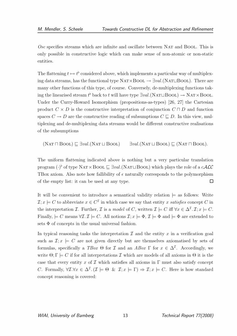
Osc specifies streams which are infinite and oscillate between Nat and Bool. This is
only possible in constructive logic which can make sense of non-atomic or non-static
entities.
The flattening t 7→ t♭ considered above, which implements a particular way of multiplex-
ing data streams, has the functional type Nat×Bool → ∃val .(Nat⊔Bool). There are
many other functions of this type, of course. Conversely, de-multiplexing functions tak-
ing the linearised stream t♭ back to t will have type ∃val .(Nat⊔Bool) → Nat×Bool.
Under the Curry-Howard Isomorphism (propositions-as-types) [26, 27] the Cartesian
product C × D is the constructive interpretation of conjunction C ⊓ D and function
spaces C → D are the constructive reading of subsumptions C ⊑ D. In this view, mul-
tiplexing and de-multiplexing data streams would be different constructive realisations
of the subsumptions
(Nat ⊓Bool) ⊑ ∃val .(Nat ⊔ Bool) ∃val .(Nat ⊔Bool) ⊑ (Nat ⊓Bool).
The uniform flattening indicated above is nothing but a very particular translation
program (·)♭ of type Nat×Bool ⊑ ∃val .(Nat⊔Bool) which plays the role of a cALC
TBox axiom. Also note how fallibility of ǫ naturally corresponds to the polymorphism
of the empty list: it can be used at any type.
It will be convenient to introduce a semantical validity relation |= as follows: Write
I; x |= C to abbreviate x ∈ CI in which case we say that entity x satisfies concept C in
the interpretation I. Further, I is a model of C, written I |= C iff ∀x ∈ ∆I . I; x |= C.
Finally, |= C means ∀I. I |= C. All notions I; x |= Φ, I |= Φ and |= Φ are extended to
sets Φ of concepts in the usual universal fashion.
In typical reasoning tasks the interpretation I and the entity x in a verification goal
such as I; x |= C are not given directly but are themselves axiomatised by sets of
formulas, specifically a TBox Θ for I and an ABox Γ for x ∈ ∆I . Accordingly, we
write Θ; Γ |= C if for all interpretations I which are models of all axioms in Θ it is the
case that every entity x of I which satisfies all axioms in Γ must also satisfy concept
C. Formally, ∀I.∀x ∈ ∆I . (I |= Θ & I; x |= Γ) ⇒ I; x |= C. Here is how standard
concept reasoning is covered:
WIAI, University of Bamberg 13 Technical Report 77(2008)
M. Mendler, S. Scheele Towards Constructive DL for Abstraction and Refinement
• Θ; {C} 6|= ⊥ iff concept C is satisfiable with respect to the TBox Θ, i.e., there
exists I with I |= Θ and non-fallible x ∈ ∆Ic such that x ∈ CI ;
• Θ; {C, D} |= ⊥ iff the concepts C and D are disjoint with respect to Θ, i.e., CI
and DI do not share any non-fallible entities in all models I of Θ;
• Θ; {C} |= D iff concept C is subsumed by concept D, i.e., for all I with I |= Θ,
CI ⊆ DI ; The same can be expressed by Θ; ∅ |= C ⊑ D (by reflexivity of �);
• Θ; ∅ |= (C ⊑ D) ⊓ (D ⊑ C) iff concepts C and D are equivalent with respect to
Θ, i.e., for all I with I |= Θ we have CI = DI . We define C ≡ D to be the
concept description (C ⊑ D) ⊓ (D ⊑ C).
It is easy to see that I |= C ⊓ D iff I |= C and I |= D. It follows that all the above
inferences can be reduced to concept subsumption Θ; {C} |= D as in classical DL.
Unlike classical DL, however, we cannot reduce concept inferences to the special form
Θ; {C} 6|= ⊥ of satisfiability. Instead, we need to implement the generalised satisfiability
check Θ; {C} 6|= D for arbitrary D. We will see in Sec. 3.2 how to build a tableau-
calculus for such generalised constructive satisfiability. Another difference to classical
DL is that whenever |= C ⊔ D then |= C or |= D. This is known as the Disjunction
Property, a definitive feature of constructive logic. In classical DL, we have |= C ⊔ ¬C
for every concept C even if neither |= C nor |= ¬C. The Disjunction Property is the
key to proof extraction for cALC (See Example 5).
cALC is related to the constructive modal logic CK (Constructive K) [28, 5, 18] as
ALC is related to the classical modal system K [11]. In cALC the classical principles
of the Excluded Middle C ⊔¬C = ⊤, double negation ¬¬C = C, the dualities ∃R.C =
¬∀R.¬C, ∀R.C = ¬∃R.¬C and Disjunctive Distribution ∃R.(C ⊔ D) = ∃R.C ⊔ ∃R.D
are no longer tautologies but non-trivial TBox statements to axiomatise specialised
classes of application scenarios (see Sec. 4). The fact that Excluded Middle, double
negation and the dualities do not hold is a feature which cALC has in common with
standard intuitionistic modal logics such as [13, 21, 14, 23]. It is well known that these
principles are non-constructive and therefore need special care. In cALC, however,
we go one step further and refute the principle of Disjunctive Distribution (and, in
fact, also the nullary version ¬3⊥) arguing that this principle is not consistent with
abstraction. Disjunctive Distribution, which corresponds to the classical 3-dual of the
normality axiom 2(A∧B) = 2A∧2B, is commonly accepted for intuitionistic modal
WIAI, University of Bamberg 14 Technical Report 77(2008)
M. Mendler, S. Scheele Towards Constructive DL for Abstraction and Refinement
logics. In other words, as a modal logic, cALC is non-normal regarding 3 and thus
proofs of decidability and finite model property for standard intuitionistic modal logics
(e.g., for IntK2,3 [15][Chap 10]) do not directly apply.
3 Constructive Proof Systems for cALC
In this section we present simple Hilbert and Gentzen-style deduction systems for cALC
which admit a direct interpretation of proofs as computations following the Curry-
Howard-Isomorphism in which the refinement relation � is treated implicitly. The
presence of the semantic refinement structure is visible in the fact that the concept
operators ⊓, ⊔, ⊑ on the one hand and ∀R, ∃R on the other are primitive and not
expressible any more in terms of each other with the help of negation as in classical
DLs. This makes sense since all have different computational meaning. According to
the Curry-Howard-Isomorphism concept descriptions are types so that, e.g., concept
conjunction ⊓ corresponds to Cartesian product ×, disjunction ⊔ to disjoint union +,
subsumption ⊑ to function spaces → (see Ex. 5).
3.1 Hilbert Calculus for cALC
(a)
1: C ⊑ (D ⊑ C)2: ((C ⊑ (D ⊑ E)) ⊑ (C ⊑ D) ⊑ (C ⊑ E))3: C ⊑ (D ⊑ (C ⊓ D))4: (C ⊓ D) ⊑ C, (C ⊓ D) ⊑ D
5: C ⊑ (C ⊔ D), D ⊑ (C ⊔ D)6: (C ⊑ E) ⊑ ((D ⊑ E) ⊑ (C ⊔ D ⊑ E))7: ⊥ ⊑ C
(b)∀K : (∀R. (C ⊑ D)) ⊑ (∀R.C ⊑ ∀R.D)∃K : (∀R. (C ⊑ D)) ⊑ (∃R.C ⊑ ∃R.D)
(c)Nec : If C is a theorem, then so is ∀R.C.MP : If C and C ⊑ D are theorems, then so is D.
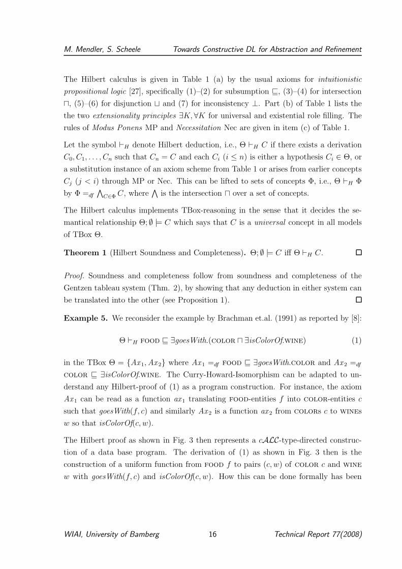
Note: Negation ¬C can be coded as C ⊑ ⊥ and ⊤ as ⊥ ⊑ ⊥.
Table 1: Hilbert Calculus for cALC.
WIAI, University of Bamberg 15 Technical Report 77(2008)
M. Mendler, S. Scheele Towards Constructive DL for Abstraction and Refinement
The Hilbert calculus is given in Table 1 (a) by the usual axioms for intuitionistic
propositional logic [27], specifically (1)–(2) for subsumption ⊑, (3)–(4) for intersection
⊓, (5)–(6) for disjunction ⊔ and (7) for inconsistency ⊥. Part (b) of Table 1 lists the
the two extensionality principles ∃K, ∀K for universal and existential role filling. The
rules of Modus Ponens MP and Necessitation Nec are given in item (c) of Table 1.
Let the symbol ⊢H denote Hilbert deduction, i.e., Θ ⊢H C if there exists a derivation
C0, C1, . . . , Cn such that Cn = C and each Ci (i ≤ n) is either a hypothesis Ci ∈ Θ, or
a substitution instance of an axiom scheme from Table 1 or arises from earlier concepts
Cj (j < i) through MP or Nec. This can be lifted to sets of concepts Φ, i.e., Θ ⊢H Φ
by Φ =df
∧
C∈Φ C, where∧
is the intersection ⊓ over a set of concepts.
The Hilbert calculus implements TBox-reasoning in the sense that it decides the se-
mantical relationship Θ; ∅ |= C which says that C is a universal concept in all models
of TBox Θ.
Theorem 1 (Hilbert Soundness and Completeness). Θ; ∅ |= C iff Θ ⊢H C.
Proof. Soundness and completeness follow from soundness and completeness of the
Gentzen tableau system (Thm. 2), by showing that any deduction in either system can
be translated into the other (see Proposition 1).
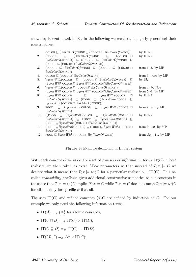
Example 5. We reconsider the example by Brachman et.al. (1991) as reported by [8]:
Θ ⊢H food ⊑ ∃goesWith.(color ⊓ ∃isColorOf.wine) (1)
in the TBox Θ = {Ax 1,Ax 2} where Ax 1 =df food ⊑ ∃goesWith.color and Ax 2 =df
color ⊑ ∃isColorOf.wine. The Curry-Howard-Isomorphism can be adapted to un-
derstand any Hilbert-proof of (1) as a program construction. For instance, the axiom
Ax 1 can be read as a function ax 1 translating food-entities f into color-entities c
such that goesWith(f, c) and similarly Ax 2 is a function ax 2 from colors c to wines
w so that isColorOf(c, w).
The Hilbert proof as shown in Fig. 3 then represents a cALC-type-directed construc-
tion of a data base program. The derivation of (1) as shown in Fig. 3 then is the
construction of a uniform function from food f to pairs (c, w) of color c and wine
w with goesWith(f, c) and isColorOf(c, w). How this can be done formally has been
WIAI, University of Bamberg 16 Technical Report 77(2008)
M. Mendler, S. Scheele Towards Constructive DL for Abstraction and Refinement
shown by Bozzato et.al. in [8]. In the following we recall (and slightly generalise) their
constructions.
1. color ⊑ (∃isColorOf.wine ⊑ (color ⊓ ∃isColorOf.wine)) by IPL 32. (color ⊑ (∃isColorOf.wine ⊑ (color ⊓
∃isColorOf.wine))) ⊑ ((color ⊑ ∃isColorOf.wine) ⊑(color ⊑ (color ⊓ ∃isColorOf.wine)))
by IPL 2
3. (color ⊑ ∃isColorOf.wine) ⊑ (color ⊑ (color ⊓∃isColorOf.wine))
from 1.,2. by MP
4. color ⊑ (color ⊓ ∃isColorOf.wine) from 3., Ax 2 by MP5. ∀goesWith.(color ⊑ (color ⊓ ∃isColorOf.wine)) ⊑
(∃goesWith.color ⊑ ∃goesWith.(color⊓∃isColorOf.wine))by ∃K
6. ∀goesWith.(color ⊑ (color ⊓ ∃isColorOf.wine)) from 4. by Nec7. (∃goesWith.color ⊑ ∃goesWith.(color⊓∃isColorOf.wine)) from 5.,6. by MP8. (∃goesWith.color ⊑ ∃goesWith.(color ⊓
∃isColorOf.wine)) ⊑ (food ⊑ (∃goesWith.color ⊑∃goesWith.(color ⊓ ∃isColorOf.wine)))
by IPL 1
9. food ⊑ (∃goesWith.color ⊑ ∃goesWith.(color ⊓∃isColorOf.wine))
from 7., 8. by MP
10. ((food ⊑ (∃goesWith.color ⊑ ∃goesWith.(color ⊓∃isColorOf.wine))) ⊑ (food ⊑ ∃goesWith.color) ⊑(food ⊑ ∃goesWith.(color ⊓ ∃isColorOf.wine)))
by IPL 2
11. (food ⊑ ∃goesWith.color) ⊑ (food ⊑ ∃goesWith.(color⊓∃isColorOf.wine))
from 9., 10. by MP
12. food ⊑ ∃goesWith.(color ⊓ ∃isColorOf.wine) from Ax1, 11. by MP
Figure 3: Example deduction in Hilbert system
With each concept C we associate a set of realisers or information terms IT(C). These
realisers are then taken as extra ABox parameters so that instead of I; x |= C we
declare what it means that I; x |= 〈α〉C for a particular realiser α ∈ IT(C). This so-
called realisability predicate gives additional constructive semantics to our concepts in
the sense that I; x |= 〈α〉C implies I; x |= C while I; x |= C does not mean I; x |= 〈α〉C
for all but only for specific α if at all.
The sets IT(C) and refined concepts 〈α〉C are defined by induction on C. For our
example we only need the following information terms:
• IT(A) =df {tt} for atomic concepts;
• IT(C ⊓ D) =df IT(C) × IT(D);
• IT(C ⊑ D) =df IT(C) → IT(D);
• IT(∃R.C) =df ∆I × IT(C);
WIAI, University of Bamberg 17 Technical Report 77(2008)
M. Mendler, S. Scheele Towards Constructive DL for Abstraction and Refinement
• IT(∀R.C) =df ∆I → IT(C).
Realisability is such that
• I; x |= 〈tt〉A iff x ∈ AI ;
• I; x |= 〈α, β〉(C ⊓ D) iff I; x |= 〈α〉C and I; x |= 〈β〉C;
• I; x |= 〈f〉(C ⊑ D) iff ∀α ∈ IT(C). I; x |= 〈α〉C ⇒ I; x |= 〈fα〉D;
• I; x |= 〈a, α〉(∃R.C) iff (x, a) ∈ RI and I; a |= 〈α〉C;
• I; x |= 〈α〉(∀R.C) iff ∀a ∈ ∆I . (x, a) ∈ RI ⇒ I; a |= 〈α a〉C.
One then shows that every proof ⊢H C generates, for any interpretation I, a function
f :∆I → IT(C) such that ∀u ∈ ∆I . I; u |= 〈fu〉C. Specifically, every of the following
Hilbert axioms IPL1:C ⊑ (D ⊑ C), IPL2:((C ⊑ (D ⊑ E)) ⊑ (C ⊑ D) ⊑ (C ⊑
E)) and IPL3:C ⊑ (D ⊑ (C ⊓ D)) is realised by a λ-term: For instance, IPL1 =df
λu.λx.λy.x, IPL2 =df λu.λx.λy.λz. (xz)(yz) and IPL3 =df λu.λx.λy. (x, y). Axiom
∃K is the function ∃K =df λu.λx.λy.(π1y, x(π1y)(π2y)). Rules of MP and Nec are
refined to
If 〈α〉C and 〈β〉(C ⊑ D) then 〈λu.(β u)(α u)〉D
If 〈α〉C then 〈λu.λx. α x〉(∀R.C).
In this way, the derivation of (1) (See Fig. 3), up to reductions in the λ-calculus,
corresponds to
prf = λu.λx.(π1(ax 1 x), (π2(ax 1 x), (π1(ax 2(π2(ax 1 x))), π2(ax 2(π2(ax 1 x))))))
which is an information term so that
∀u. I; u |= 〈prf u〉(food ⊑ ∃goesWith.(color ⊓ ∃isColorOf.wine))
assuming that ∀u. I; u |= 〈ax 1 u〉Ax 1 and ∀u. I; u |= 〈ax 2 u〉Ax 2. Such realisers ax 1,
ax 2 can be obtained from a concrete ABox [8].
Either they arise as proof terms themselves, or they are induced from a particular se-
mantic ABox, as shown by Bozzato [8]. For instance, take the (classical) interpretation
I described by
WIAI, University of Bamberg 18 Technical Report 77(2008)
M. Mendler, S. Scheele Towards Constructive DL for Abstraction and Refinement
∆I =df {barolo, chardonnay, red, white, fish, meat},
wineI =df {barolo, chardonnay},
colorI =df {red, white},
foodI =df {fish, meat},
isColorOfI =df {(red, barolo), (white, chardonnay)},
goesWithI =df {(meat, red), (fish, white)}.
In this interpretation (or ABox) I the information terms ax 1, ax 2 can be chosen such
that
ax 1 =df λu.λx.case u of [meat → (red, tt) | fish → (white, tt)]
ax 2 =df λu.λx.case u of [red → (barolo, tt) | white → (chardonnay, tt)]
where
ax 1 ∈ ∆I → IT(food ⊑ ∃goesWith.color), and
ax 2 ∈ ∆I → IT(color ⊑ ∃isColorOf.wine).
These express the constructive content of Ax 1, Ax 2 in I.
Note that the equivalent tableau system specified in the next Sec. 3.2 would allow us
to obtain prf more efficiently. Also, instead of reading the TBox axioms Ax 1 and Ax 2
as functions (as done in [8]) we can also interpret them constructively as relations, i.e.,
data-base tables.
3.2 Gentzen Tableau Calculus for cALC
The Hilbert calculus for cALC does not lend itself to efficient implementations. Much
better suited for automated reasoning in practical applications are refutation or tableau
calculi. Refutation or tableau calculi play an important role in automated reasoning.
These combine both goal-directed proof-search and counter-model construction. In this
section we will present such a tableau system for cALC based on Gentzen-style sequents.
In contrast to tableau systems for classical DL it is consistent with the Curry-Howard
Isomorphism and thus permits proof-extraction. In contrast to natural deduction sys-
tems such as [8], Gentzen-systems not only support the constructive interpretation of
proofs as λ-terms but also formalise tableau-style refutation procedures.
WIAI, University of Bamberg 19 Technical Report 77(2008)
M. Mendler, S. Scheele Towards Constructive DL for Abstraction and Refinement
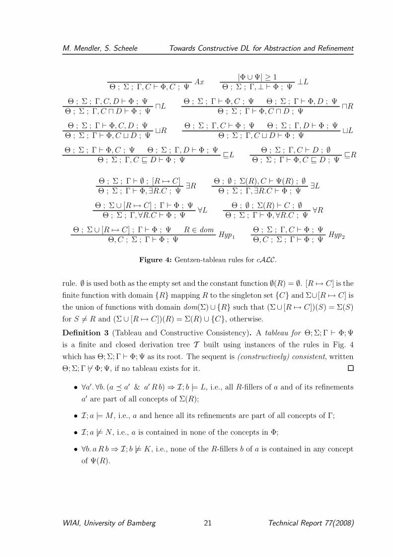
The tableau calculus manipulates Gentzen-style sequents Θ; Σ; Γ ⊢ Φ; Ψ, where Θ, Γ, Φ
are sets of concepts, not necessarily finite, and Σ, Ψ are partial functions mapping role
names R ∈ NR to sets of concepts Σ(R), Ψ(R) which may be infinite, too. The domains
of the latter functions are assumed to be finite and identical. We call dom = dom(Σ) =
dom(Ψ) ⊆ NR the domain of the sequent. A sequent Θ; Σ; Γ ⊢ Φ; Ψ formalises and
refines the semantic validity relationship Θ; Γ |= Φ (see page 13) by extra constraints
Σ, Ψ as follows: Θ is the TBox which are model assumptions. The ABox is given
by the sets Σ, Γ, Φ, Ψ of the sequent. These encode information about individual
entities relative to Θ. The first, Σ, Γ specify what we want an entity to satisfy and the
latter Φ, Ψ what we do not want them to satisfy. The fact that we sandwich entities
between explicit positive and negative constraints is the novel constructive aspect of
the following Definition 2:
Definition 2 (Constructive Satisfiability). Let I = (∆I ,�I ,⊥I , ·I) be an interpre-
tation and a ∈ ∆I an entity in I. We say that the pair (I, a) satisfies a sequent
Θ; Σ; Γ ⊢ Φ; Ψ if I is a model of Θ, I |= Θ, and for all R ∈ dom, L ∈ Σ(R), M ∈ Γ,
N ∈ Φ, K ∈ Ψ(R):
• ∀a′. ∀b. (a � a′ & a′ R b) ⇒ I; b |= L, i.e., all R-fillers of a and of its refinements
a′ are part of all concepts of Σ(R);
• I; a |= M , i.e., a and hence all its refinements are part of all concepts of Γ;
• I; a 6|= N , i.e., a is contained in none of the concepts in Φ;
• ∀b. a R b ⇒ I; b 6|= K, i.e., none of the R-fillers b of a is contained in any concept
of Ψ(R).
A sequent Θ; Σ; Γ ⊢ Φ; Ψ is (constructively) satisfiable, written Θ; Σ; Γ 6|= Φ; Ψ, iff there
exists an interpretation I and entity a ∈ ∆I such that (I, a) satisfies the sequent.
The purpose of a tableau or refutation proof is to establish that an entity specification
presented as a sequent is not satisfiable. On the other hand, if no closed tableau can be
found and the calculus is complete then the failed proof search implies the existence of
a satisfying entity. Our tableau calculus for cALC is given by the rules seen in Fig. 4.
In all rules of Fig. 4, the hypotheses Θ, Σ(R), Γ and conclusions Φ, Ψ(R) are treated
as sets rather than lists. For instance, Γ, C ⊑ D in rule ⊑L is Γ ∪ {C ⊑ D}. Hence, if
C ⊑ D ∈ Γ then Γ in the premise of ⊑L is identical to Γ, C ⊑ D in the conclusion of the
WIAI, University of Bamberg 20 Technical Report 77(2008)
M. Mendler, S. Scheele Towards Constructive DL for Abstraction and Refinement
AxΘ ; Σ ; Γ, C ⊢ Φ, C ; Ψ
|Φ ∪ Ψ| ≥ 1⊥L
Θ ; Σ ; Γ,⊥ ⊢ Φ ; Ψ
Θ ; Σ ; Γ, C, D ⊢ Φ ; Ψ⊓L
Θ ; Σ ; Γ, C ⊓ D ⊢ Φ ; ΨΘ ; Σ ; Γ ⊢ Φ, C ; Ψ Θ ; Σ ; Γ ⊢ Φ, D ; Ψ
⊓RΘ ; Σ ; Γ ⊢ Φ, C ⊓ D ; Ψ
Θ ; Σ ; Γ ⊢ Φ, C, D ; Ψ⊔R
Θ ; Σ ; Γ ⊢ Φ, C ⊔ D ; ΨΘ ; Σ ; Γ, C ⊢ Φ ; Ψ Θ ; Σ ; Γ, D ⊢ Φ ; Ψ
⊔LΘ ; Σ ; Γ, C ⊔ D ⊢ Φ ; Ψ
Θ ; Σ ; Γ ⊢ Φ, C ; Ψ Θ ; Σ ; Γ, D ⊢ Φ ; Ψ⊑L
Θ ; Σ ; Γ, C ⊑ D ⊢ Φ ; ΨΘ ; Σ ; Γ, C ⊢ D ; ∅
⊑RΘ ; Σ ; Γ ⊢ Φ, C ⊑ D ; Ψ
Θ ; Σ ; Γ ⊢ ∅ ; [R 7→ C]∃R
Θ ; Σ ; Γ ⊢ Φ, ∃R.C ; ΨΘ ; ∅ ; Σ(R), C ⊢ Ψ(R) ; ∅
∃LΘ ; Σ ; Γ, ∃R.C ⊢ Φ ; Ψ
Θ ; Σ ∪ [R 7→ C] ; Γ ⊢ Φ ; Ψ∀L
Θ ; Σ ; Γ, ∀R.C ⊢ Φ ; ΨΘ ; ∅ ; Σ(R) ⊢ C ; ∅
∀RΘ ; Σ ; Γ ⊢ Φ, ∀R.C ; Ψ
Θ ; Σ ∪ [R 7→ C] ; Γ ⊢ Φ ; Ψ R ∈ domHyp1Θ, C ; Σ ; Γ ⊢ Φ ; Ψ
Θ ; Σ ; Γ, C ⊢ Φ ; ΨHyp2Θ, C ; Σ ; Γ ⊢ Φ ; Ψ
Figure 4: Gentzen-tableau rules for cALC.
rule. ∅ is used both as the empty set and the constant function ∅(R) = ∅. [R 7→ C] is the
finite function with domain {R} mapping R to the singleton set {C} and Σ∪[R 7→ C] is
the union of functions with domain dom(Σ)∪ {R} such that (Σ∪ [R 7→ C])(S) = Σ(S)
for S 6= R and (Σ ∪ [R 7→ C])(R) = Σ(R) ∪ {C}, otherwise.
Definition 3 (Tableau and Constructive Consistency). A tableau for Θ; Σ; Γ ⊢ Φ; Ψ
is a finite and closed derivation tree T built using instances of the rules in Fig. 4
which has Θ; Σ; Γ ⊢ Φ; Ψ as its root. The sequent is (constructively) consistent, written
Θ; Σ; Γ 6⊢ Φ; Ψ, if no tableau exists for it.
• ∀a′. ∀b. (a � a′ & a′ R b) ⇒ I; b |= L, i.e., all R-fillers of a and of its refinements
a′ are part of all concepts of Σ(R);
• I; a |= M , i.e., a and hence all its refinements are part of all concepts of Γ;
• I; a 6|= N , i.e., a is contained in none of the concepts in Φ;
• ∀b. a R b ⇒ I; b 6|= K, i.e., none of the R-fillers b of a is contained in any concept
of Ψ(R).
WIAI, University of Bamberg 21 Technical Report 77(2008)
M. Mendler, S. Scheele Towards Constructive DL for Abstraction and Refinement
Our calculus is formulated in the spirit of Gentzen with left introduction rules ⊓L, ⊔L,
⊑L, ∀L, ∃L and right introduction rules ⊓R, ⊔R, ⊑R, ∀R, ∃R for each logical con-
nective. These rules can be interpreted not only as tableau-style refutation steps but
also have computational meaning. Specifically, the left rules correspond to input de-
composition (pattern matching) and the right rules generate output information terms
(data constructors). The Gentzen style presentation also lends itself to a natural game-
theoretic interpretation. These features are distinct advantages over natural deduction
systems such as presented in [8]. Note that there is no right intro rule ⊥R, which is not
needed. One shows for the system in Fig. 4 that whenever Θ; Σ; Γ ⊢ Φ; Ψ is derivable
then also Θ; Σ; Γ ⊢ Φ,⊥; Ψ is derivable which is basically ⊥L.
It is possible to treat negated concepts directly by the following left and right introduc-
tion rules ¬L resp. ¬R which can be derived from the rules in Fig. 4. Since negation
is encoded as ¬C ≡ C ⊑ ⊥ the rule ¬L is simply a combination of the rules ⊑L and
⊥L. Rule ¬R is an instance of rule ⊑R.
Θ ; Σ ; Γ ⊢ Φ, C ; Ψ | Φ ∪ Ψ |≥ 1¬L
Θ ; Σ ; Γ,¬C ⊢ Φ ; ΨΘ ; Σ ; Γ, C ⊢ ⊥ ; ∅
¬RΘ ; Σ ; Γ ⊢ Φ,¬C ; Ψ
Proposition 1. The Hilbert and Tableau calculi are equivalent. For any TBox Θ and
set of concepts Φ we have Θ ⊢H Φ iff the sequent Θ; ∅; ∅ ⊢ Φ; ∅ has a tableau derivation
(i.e., is inconsistent).
Proof. This is done by showing that the tableau system can simulate the Hilbert de-
ductions, i.e., we show that if Θ ⊢H C then there exists a closed tableau for the sequent
Θ; ∅; ∅ ⊢ C; ∅. Thereof we obtain soundness of Hilbert from soundness of Gentzen
(Thm. 2).
In the other direction we have to show that if there is a closed tableau for a sequent then
each such sequent can be derived in the Hilbert system in closed form as an implication.
The proof is by induction on the structure of a closed tableau. The details of the proof
can be found in the appendix.
Theorem 2 (Strong Soundness and Completeness). A sequent is satisfiable iff it is
consistent, i.e., Θ; Σ; Γ 6|= Φ; Ψ ⇔ Θ; Σ; Γ 6⊢ Φ; Ψ.
WIAI, University of Bamberg 22 Technical Report 77(2008)
M. Mendler, S. Scheele Towards Constructive DL for Abstraction and Refinement
Proof. For soundness we show for each derivation rule in Fig. 4 that if the conclusion
is satisfiable then at least one of the premises of the rule is satisfiable, too. For the
completeness direction we show that for any consistent sequent there exists a canon-
ical constructive model that satisfies the sequent. The detailed proof is given in the
appendix.
A sequent Θ; Σ; Γ ⊢ Φ; Ψ is finite if it has a finite domain and for all R ∈ dom the sets
Σ(R), Ψ(R) as well as Θ, Γ, Φ are finite as well. The tableau rules in Fig. 4 induce
a decidable deduction system for finite sequents. In fact, the proof of Thm. 2 shows
that finite counter-models can be obtained essentially by unfolding unprovable finite
end-sequents.
Theorem 3 (Finite Model Property & Decidability). A finite sequent is satisfiable iff
it is satisfiable in a finite interpretation. Consistency of finite sequents is decidable.
Proof. Decidability is obtained by the simple fact that the tableau rules in Fig. 4 have
the sub-formula property: All formulas in the premises of a rule are (not necessarily
proper) sub-formulas of formulas in the conclusion. Also, the domain of a premise
sequent is extended at most by a role appearing in concepts of the conclusion sequent
(as in rules ∃R, ∀L or is already part the domains). In rule Hyp1 a role already existing
in the domain of the conclusion sequent is updated. Thus, the sizes of the domains and
formula sets in a tableau are bounded by the root sequent. More specifically, if we are
searching for a closed tableau of a finite sequent 〈Θ; Σ; Γ⊢Φ; Ψ〉 then we only ever need
to consider tableaux with nodes formed from those (sub-)concepts and roles contained
in 〈Θ; Σ; Γ⊢Φ; Ψ〉. Since there are only a finite number of such nodes and the tableau
rules are finitely branching, there are only a finite number of possible tableaux with
finite root sequent 〈Θ; Σ; Γ⊢Φ; Ψ〉. These can be enumerated and checked effectively
in bounded time.
Finite Model Property follows from the completeness direction of Thm. 2 refined by
showing that the canonical model which satisfies a given finite sequent is finite.
Example 6. Auditors usually check if financial transactions expensed on different
kinds of accounts are, depending on their type, in compliance with regulations and
accounting standards. For example, a financial transaction trans may be expensed
on an Account or by refinement on CashBox, say under special instructions from the
WIAI, University of Bamberg 23 Technical Report 77(2008)
M. Mendler, S. Scheele Towards Constructive DL for Abstraction and Refinement
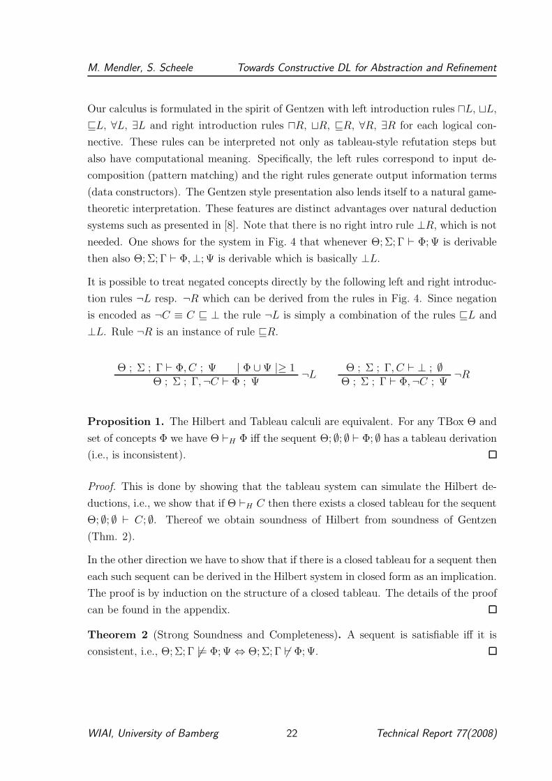
manager. A corresponding ABox I is given in Fig. 5 with roles NR = {expOn} and
concepts NC = {acc,cash}.
b b
b b
trans trans′
CASHACC
�
expOnexpOn
Figure 5: ABox I
There may be a TBox Θ specifying general facts
about the role and concepts in I such as acc ⊑
¬cash or ∀expOn.(acc ⊔ cash). The particu-
lar ABox structure of Fig. 5 can be specified by
the sequent Θ; Σ; Γ ⊢ Φ; Ψ where Σ(expOn) = ∅,
Γ = {∃expOn.(acc ⊔ cash)}, Φ = {∃expOn.acc}
and Ψ(expOn) = {cash}. Note that the ABox
specification Θ; Σ; Γ ⊢ Φ; Ψ is inconsistent with the
classical principle of ∃-distributivity. E.g., if we add
∃expOn.acc ⊔ ∃expOn.cash to Σ then the sequent becomes unsatisfiable.
We have seen before how the following sequent specifies the ABox in Fig. 5.
∅; ∅; ∃expOn.(acc ⊔ cash) ⊢ ∃expOn.acc; [expOn 7→ cash]
Since this sequent is satisfiable there cannot be a closed tableau for it (Thm. 2). As
with classical tableaux the ABox model in Fig. 5 can be extracted systematically from
the unsuccessful attempt to prove the sequent using the tableau rules.
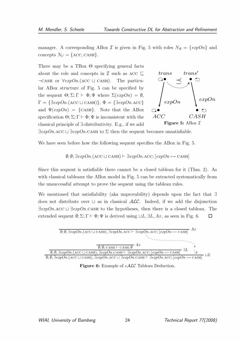
We mentioned that satisfiability (aka unprovability) depends upon the fact that ∃
does not distribute over ⊔ as in classical ALC. Indeed, if we add the disjunction
∃expOn.acc ⊔ ∃expOn.cash to the hypotheses, then there is a closed tableau. The
extended sequent ∅; Σ; Γ ⊢ Φ; Ψ is derived using ⊔L, ∃L,Ax , as seen in Fig. 6.
Ax∅; ∅; ∃expOn.(acc ⊔ cash), ∃expOn.acc ⊢ ∃expOn.acc; [expOn 7→ cash]
Ax∅; ∅;cash ⊢ cash; ∅
∃L∅; ∅; ∃expOn.(acc ⊔ cash), ∃expOn.cash ⊢ ∃expOn.acc; [expOn 7→ cash]
...π⊔L
∅; ∅; ∃expOn.(acc ⊔ cash), ∃expOn.acc ⊔ ∃expOn.cash ⊢ ∃expOn.acc; [expOn 7→ cash]
Figure 6: Example of cALC Tableau Deduction.
WIAI, University of Bamberg 24 Technical Report 77(2008)
M. Mendler, S. Scheele Towards Constructive DL for Abstraction and Refinement
Example 7. Fig. 7 gives tableau proofs of the Hilbert axioms ∀K and ∃K.
∅ ; ∅ ; A ⊢ A ; ∅ ∅ ; ∅ ; B, A ⊢ B ; ∅∅ ; ∅ ; A ⊑ B, A ⊢ B ; ∅
∀R∅ ; [R 7→ A ⊑ B, A] ; ∅ ⊢ ∀R.B ; ∅
∀L∅ ; [R 7→ A ⊑ B] ; ∀R.A ⊢ ∀R.B ; ∅
∀L∅ ; ∅ ; ∀R.(A ⊑ B), ∀R.A ⊢ ∀R.B ; ∅∅ ; ∅ ; ∀R.(A ⊑ B) ⊢ ∀R.A ⊑ ∀R.B ; ∅
∅ ; ∅ ; ∅ ⊢ ∀R.(A ⊑ B) ⊑ (∀R.A ⊑ ∀R.B) ; ∅
∅ ; ∅ ; A ⊢ A ; ∅ ∅ ; ∅ ; B, A ⊢ B ; ∅∅ ; ∅ ; A ⊑ B, A ⊢ B ; ∅
∃L∅ ; [R 7→ A ⊑ B] ; ∃R.A ⊢ ∅ ; [R 7→ B]
∃R∅ ; [R 7→ A ⊑ B] ; ∃R.A ⊢ ∃R.B ; ∅
∀L∅ ; ∅ ; ∀R.(A ⊑ B), ∃R.A ⊢ ∃R.B ; ∅∅ ; ∅ ; ∀R.(A ⊑ B) ⊢ ∃R.A ⊑ ∃R.B ; ∅
∅ ; ∅ ; ∅ ⊢ ∀R.(A ⊑ B) ⊑ (∃R.A ⊑ ∃R.B) ; ∅
Figure 7: Hilbert axioms ∃K, ∀K derived in the tableau calculus.
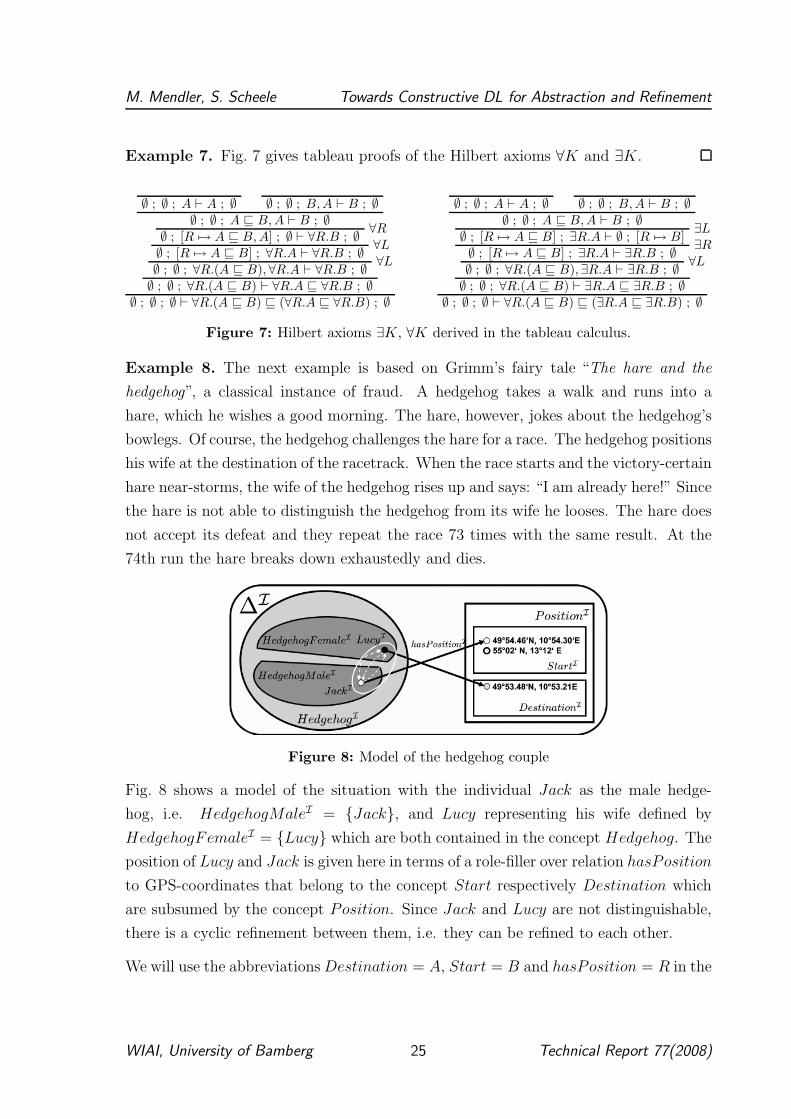
Example 8. The next example is based on Grimm’s fairy tale “The hare and the
hedgehog”, a classical instance of fraud. A hedgehog takes a walk and runs into a
hare, which he wishes a good morning. The hare, however, jokes about the hedgehog’s
bowlegs. Of course, the hedgehog challenges the hare for a race. The hedgehog positions
his wife at the destination of the racetrack. When the race starts and the victory-certain
hare near-storms, the wife of the hedgehog rises up and says: “I am already here!” Since
the hare is not able to distinguish the hedgehog from its wife he looses. The hare does
not accept its defeat and they repeat the race 73 times with the same result. At the
74th run the hare breaks down exhaustedly and dies.
Figure 8: Model of the hedgehog couple
Fig. 8 shows a model of the situation with the individual Jack as the male hedge-
hog, i.e. HedgehogMaleI = {Jack}, and Lucy representing his wife defined by
HedgehogFemaleI = {Lucy} which are both contained in the concept Hedgehog. The
position of Lucy and Jack is given here in terms of a role-filler over relation hasPosition
to GPS-coordinates that belong to the concept Start respectively Destination which
are subsumed by the concept Position. Since Jack and Lucy are not distinguishable,
there is a cyclic refinement between them, i.e. they can be refined to each other.
We will use the abbreviations Destination = A, Start = B and hasPosition = R in the
WIAI, University of Bamberg 25 Technical Report 77(2008)
M. Mendler, S. Scheele Towards Constructive DL for Abstraction and Refinement
following. Based on our model in Fig. 8 we can show that the existential quantifier does
not distribute over ⊔. If ∃R would distribute over ⊔ as it does in classical ALC then this
would imply that we can find a derivation for ∃R.(A⊔B),¬(∃R.A⊔∃R.B) ⊢ ⊥: If the
first hypothesis ∃R.(A ⊔B) of the sequent implies ∃R.A ⊔ ∃R.B, then this contradicts
the second hypothesis ¬(∃R.A ⊔ ∃R.B) which implies ⊥.
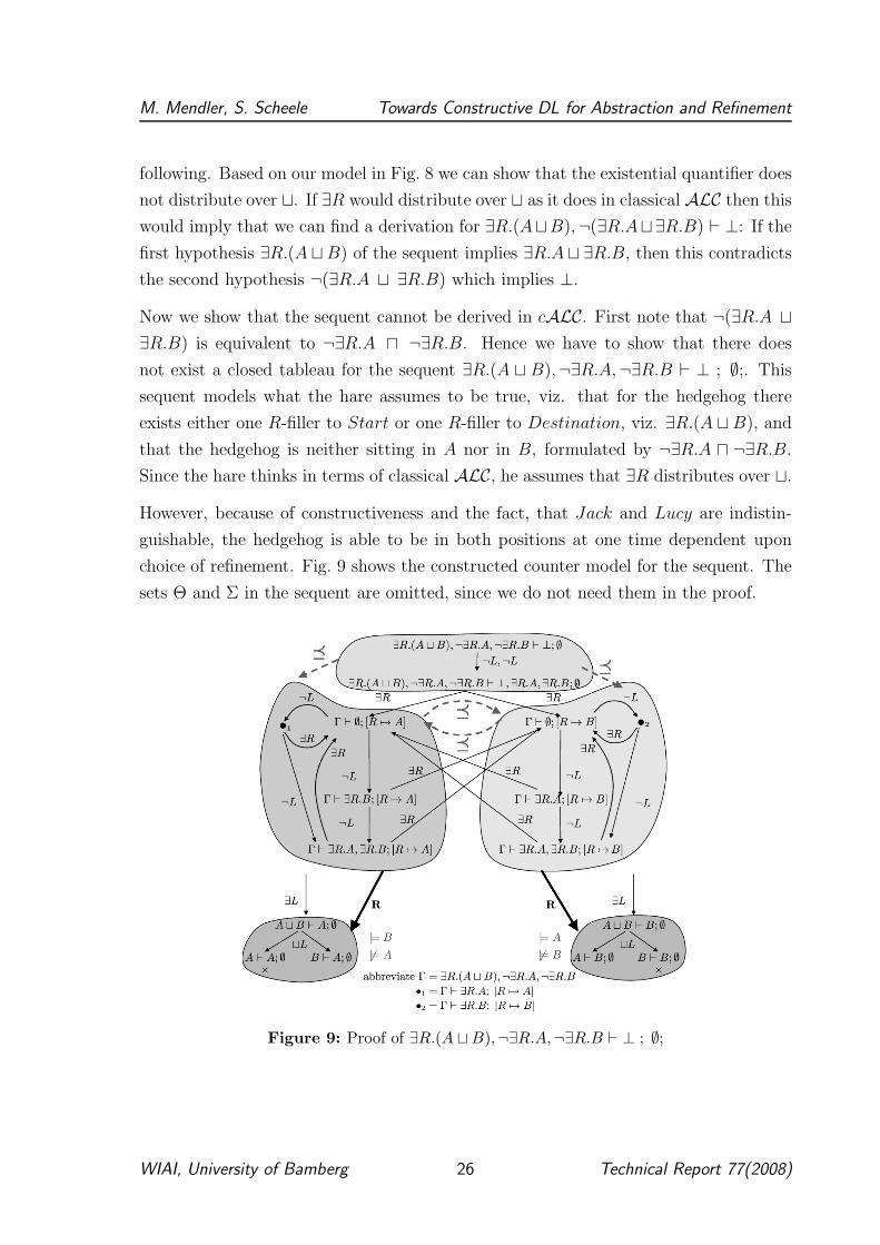
Now we show that the sequent cannot be derived in cALC. First note that ¬(∃R.A ⊔
∃R.B) is equivalent to ¬∃R.A ⊓ ¬∃R.B. Hence we have to show that there does
not exist a closed tableau for the sequent ∃R.(A ⊔ B),¬∃R.A,¬∃R.B ⊢ ⊥ ; ∅;. This
sequent models what the hare assumes to be true, viz. that for the hedgehog there
exists either one R-filler to Start or one R-filler to Destination, viz. ∃R.(A ⊔ B), and
that the hedgehog is neither sitting in A nor in B, formulated by ¬∃R.A ⊓ ¬∃R.B.
Since the hare thinks in terms of classical ALC, he assumes that ∃R distributes over ⊔.
However, because of constructiveness and the fact, that Jack and Lucy are indistin-
guishable, the hedgehog is able to be in both positions at one time dependent upon
choice of refinement. Fig. 9 shows the constructed counter model for the sequent. The
sets Θ and Σ in the sequent are omitted, since we do not need them in the proof.
Figure 9: Proof of ∃R.(A ⊔ B),¬∃R.A,¬∃R.B ⊢ ⊥ ; ∅;
WIAI, University of Bamberg 26 Technical Report 77(2008)
M. Mendler, S. Scheele Towards Constructive DL for Abstraction and Refinement
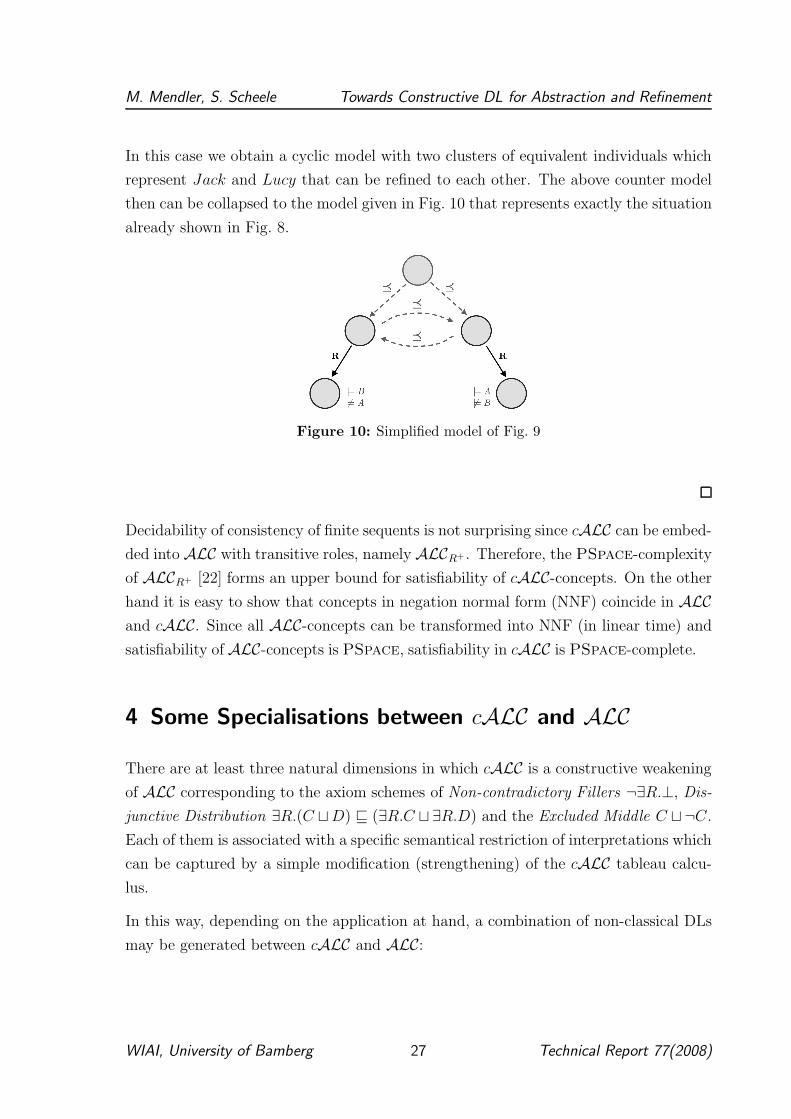
In this case we obtain a cyclic model with two clusters of equivalent individuals which
represent Jack and Lucy that can be refined to each other. The above counter model
then can be collapsed to the model given in Fig. 10 that represents exactly the situation
already shown in Fig. 8.
Figure 10: Simplified model of Fig. 9
Decidability of consistency of finite sequents is not surprising since cALC can be embed-
ded into ALC with transitive roles, namely ALCR+ . Therefore, the PSpace-complexity
of ALCR+ [22] forms an upper bound for satisfiability of cALC-concepts. On the other
hand it is easy to show that concepts in negation normal form (NNF) coincide in ALC
and cALC. Since all ALC-concepts can be transformed into NNF (in linear time) and
satisfiability of ALC-concepts is PSpace, satisfiability in cALC is PSpace-complete.
4 Some Specialisations between cALC and ALC
There are at least three natural dimensions in which cALC is a constructive weakening
of ALC corresponding to the axiom schemes of Non-contradictory Fillers ¬∃R.⊥, Dis-
junctive Distribution ∃R.(C ⊔D) ⊑ (∃R.C ⊔ ∃R.D) and the Excluded Middle C ⊔¬C.
Each of them is associated with a specific semantical restriction of interpretations which
can be captured by a simple modification (strengthening) of the cALC tableau calcu-
lus.
In this way, depending on the application at hand, a combination of non-classical DLs
may be generated between cALC and ALC:
WIAI, University of Bamberg 27 Technical Report 77(2008)
M. Mendler, S. Scheele Towards Constructive DL for Abstraction and Refinement
Interpretations without fallible elements, i.e., ⊥I = ∅, can be axiomatised by the scheme
¬∃R.⊥ which says that any entity can always be refined so it becomes fully defined
for role R, i.e., all its R-fillers (if they exist) are non-fallible. In fact, the absence
of axiom ¬∃R.⊥ is the only effect of fallibility. It indicates the existence of entities
all of whose refinements have fallible R-fillers. One can show that if an interpretation
I = (∆I ,�I ,⊥I , ·I) satisfies ¬∃R.⊥ then the set ⊥I is redundant in the sense that there
is a stripped interpretation Is = (∆Is,�Is ,⊥Is, ·Is) such that ∆Is =df ∆Ic = ∆I \ ⊥I ,
�Is=df�I , ⊥Is =df ∅ so that for all concepts C we have CIs = CI \ ⊥I . This means
that as long as we are only interested in non-fallible entities, I and Is are identical. To
achieve this one defines ·Is so that AIs =df AI \ ⊥I for A ∈ NC and for all x, y ∈ ∆Is
and R ∈ NR we put xRIs y iff xRI y, or ∃y′, x′. xRIy′ ∈ ⊥I & x �I x′ RI y. If we
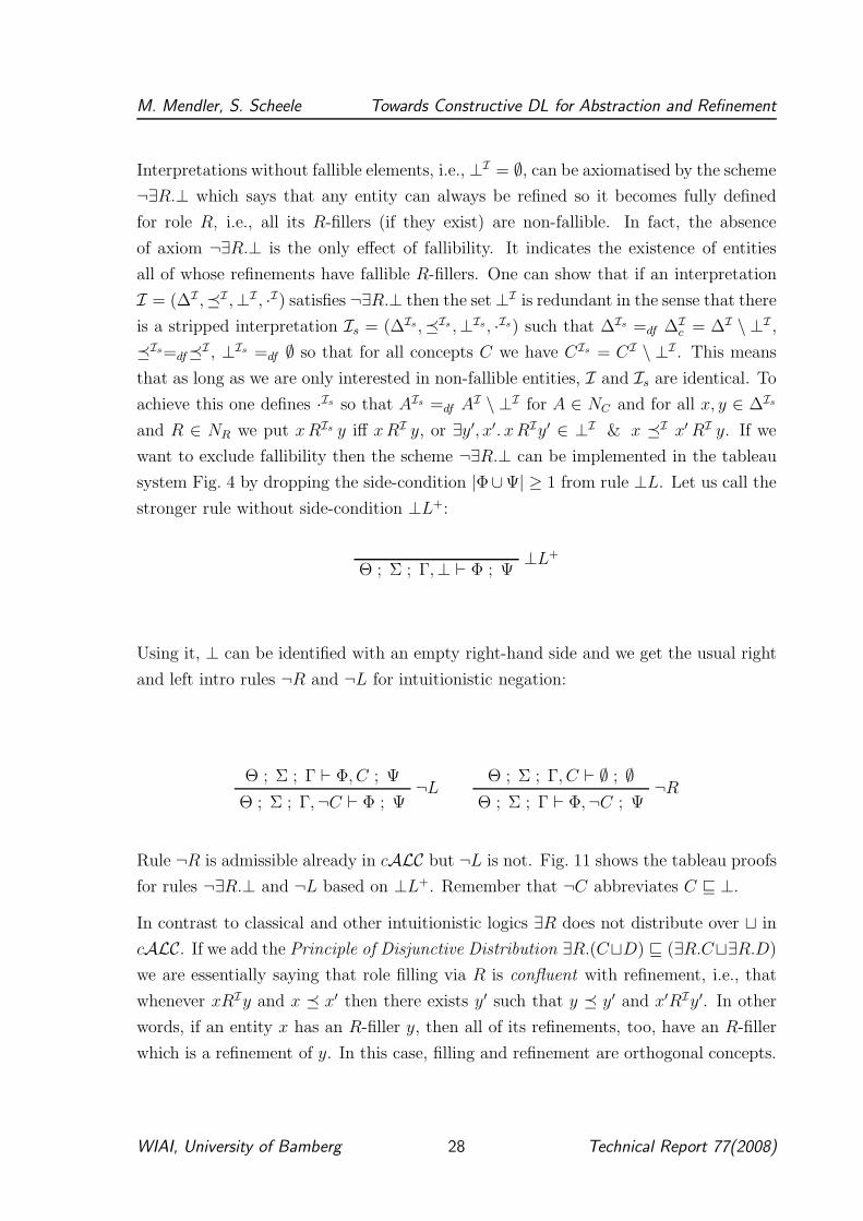
want to exclude fallibility then the scheme ¬∃R.⊥ can be implemented in the tableau
system Fig. 4 by dropping the side-condition |Φ∪Ψ| ≥ 1 from rule ⊥L. Let us call the
stronger rule without side-condition ⊥L+:
⊥L+
Θ ; Σ ; Γ,⊥ ⊢ Φ ; Ψ
Using it, ⊥ can be identified with an empty right-hand side and we get the usual right
and left intro rules ¬R and ¬L for intuitionistic negation:
Θ ; Σ ; Γ ⊢ Φ, C ; Ψ¬L
Θ ; Σ ; Γ,¬C ⊢ Φ ; Ψ
Θ ; Σ ; Γ, C ⊢ ∅ ; ∅¬R
Θ ; Σ ; Γ ⊢ Φ,¬C ; Ψ
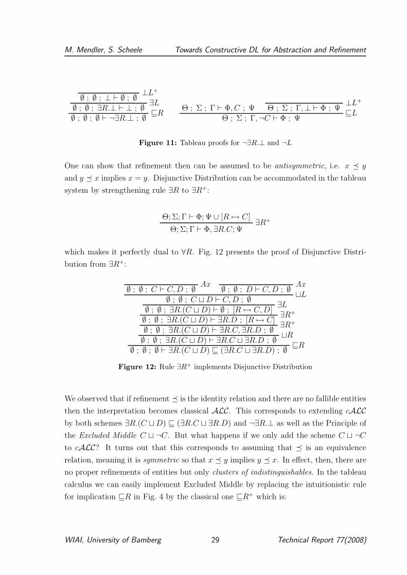
Rule ¬R is admissible already in cALC but ¬L is not. Fig. 11 shows the tableau proofs
for rules ¬∃R.⊥ and ¬L based on ⊥L+. Remember that ¬C abbreviates C ⊑ ⊥.
In contrast to classical and other intuitionistic logics ∃R does not distribute over ⊔ in
cALC. If we add the Principle of Disjunctive Distribution ∃R.(C⊔D) ⊑ (∃R.C⊔∃R.D)
we are essentially saying that role filling via R is confluent with refinement, i.e., that
whenever xRIy and x � x′ then there exists y′ such that y � y′ and x′RIy′. In other
words, if an entity x has an R-filler y, then all of its refinements, too, have an R-filler
which is a refinement of y. In this case, filling and refinement are orthogonal concepts.
WIAI, University of Bamberg 28 Technical Report 77(2008)
M. Mendler, S. Scheele Towards Constructive DL for Abstraction and Refinement
⊥L+
∅ ; ∅ ; ⊥ ⊢ ∅ ; ∅∃L
∅ ; ∅ ; ∃R.⊥ ⊢ ⊥ ; ∅⊑R
∅ ; ∅ ; ∅ ⊢ ¬∃R.⊥ ; ∅Θ ; Σ ; Γ ⊢ Φ, C ; Ψ
⊥L+
Θ ; Σ ; Γ,⊥ ⊢ Φ ; Ψ⊑L
Θ ; Σ ; Γ,¬C ⊢ Φ ; Ψ
Figure 11: Tableau proofs for ¬∃R.⊥ and ¬L
One can show that refinement then can be assumed to be antisymmetric, i.e. x � y
and y � x implies x = y. Disjunctive Distribution can be accommodated in the tableau
system by strengthening rule ∃R to ∃R+:
Θ; Σ; Γ ⊢ Φ; Ψ ∪ [R 7→ C]∃R+
Θ; Σ; Γ ⊢ Φ, ∃R.C; Ψ
which makes it perfectly dual to ∀R. Fig. 12 presents the proof of Disjunctive Distri-
bution from ∃R+:
Ax∅ ; ∅ ; C ⊢ C, D ; ∅
Ax∅ ; ∅ ; D ⊢ C, D ; ∅
⊔L∅ ; ∅ ; C ⊔ D ⊢ C, D ; ∅
∃L∅ ; ∅ ; ∃R.(C ⊔ D) ⊢ ∅ ; [R 7→ C, D]
∃R+
∅ ; ∅ ; ∃R.(C ⊔ D) ⊢ ∃R.D ; [R 7→ C]∃R+
∅ ; ∅ ; ∃R.(C ⊔ D) ⊢ ∃R.C, ∃R.D ; ∅⊔R
∅ ; ∅ ; ∃R.(C ⊔ D) ⊢ ∃R.C ⊔ ∃R.D ; ∅⊑R
∅ ; ∅ ; ∅ ⊢ ∃R.(C ⊔ D) ⊑ (∃R.C ⊔ ∃R.D) ; ∅
Figure 12: Rule ∃R+ implements Disjunctive Distribution
We observed that if refinement � is the identity relation and there are no fallible entities
then the interpretation becomes classical ALC. This corresponds to extending cALC
by both schemes ∃R.(C ⊔D) ⊑ (∃R.C ⊔ ∃R.D) and ¬∃R.⊥ as well as the Principle of
the Excluded Middle C ⊔ ¬C. But what happens if we only add the scheme C ⊔ ¬C
to cALC? It turns out that this corresponds to assuming that � is an equivalence
relation, meaning it is symmetric so that x � y implies y � x. In effect, then, there are
no proper refinements of entities but only clusters of indistinguishables. In the tableau
calculus we can easily implement Excluded Middle by replacing the intuitionistic rule
for implication ⊑R in Fig. 4 by the classical one ⊑R+ which is:
WIAI, University of Bamberg 29 Technical Report 77(2008)
M. Mendler, S. Scheele Towards Constructive DL for Abstraction and Refinement
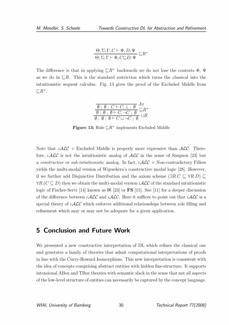
Θ; Σ; Γ, C ⊢ Φ, D; Ψ⊑R+
Θ; Σ; Γ ⊢ Φ, C⊑D; Ψ
The difference is that in applying ⊑R+ backwards we do not lose the contexts Φ, Ψ
as we do in ⊑R. This is the standard restriction which turns the classical into the
intuitionistic sequent calculus. Fig. 13 gives the proof of the Excluded Middle from
⊑R+.
Ax∅ ; ∅ ; C ⊢ C,⊥ ; ∅
⊑R+
∅ ; ∅ ; ∅ ⊢ C,¬C ; ∅⊔R
∅ ; ∅ ; ∅ ⊢ C ⊔ ¬C ; ∅
Figure 13: Rule ⊑R+ implements Excluded Middle
Note that cALC + Excluded Middle is properly more expressive than ALC. There-
fore, cALC is not the intuitionistic analog of ALC in the sense of Simpson [23] but
a constructive or sub-intuitionistic analog. In fact, cALC + Non-contradictory Fillers
yields the multi-modal version of Wijesekera’s constructive modal logic [28]. However,
if we further add Disjunctive Distribution and the axiom scheme (∃R.C ⊑ ∀R.D) ⊑
∀R.(C ⊑ D) then we obtain the multi-modal version iALC of the standard intuitionistic
logic of Fischer-Servi [14] known as IK [23] or FS [15]. See [11] for a deeper discussion
of the difference between cALC and iALC. Here it suffices to point out that iALC is a
special theory of cALC which enforces additional relationships between role filling and
refinement which may or may not be adequate for a given application.
5 Conclusion and Future Work
We presented a new constructive interpretation of DL which refines the classical one
and generates a family of theories that admit computational interpretations of proofs
in line with the Curry-Howard Isomorphism. This new interpretation is consistent with
the idea of concepts comprising abstract entities with hidden fine-structure. It supports
intensional ABox and TBox theories with semantic slack in the sense that not all aspects
of the low-level structure of entities can necessarily be captured by the concept language.
WIAI, University of Bamberg 30 Technical Report 77(2008)
M. Mendler, S. Scheele Towards Constructive DL for Abstraction and Refinement
This gives rise to the notion of constructive satisfiability and a stronger form of OWA,
which we tentatively call the Evolving Open World Assumption.
In this work we applied this interpretation to ALC as the core DL obtaining cALC to-
gether with sound and complete Hilbert and Tableau deduction systems. The semantics
is general enough that it should be applicable to other DLs, too. It is conservative in
that all constructions of cALC are sound in ALC. The point is that cALC does not
permit constructions which are incompatible with refinement. We have given examples
where ALC would not be adequate. cALC enjoys semantical robustness and admits
decidable tableau with proof extraction and counter-model construction. Where the
application supports it we can specialise cALC back towards ALC by adding axioms
or strengthen some tableau rules suitably, as discussed.
We aim to extend cALC for the domain of mass data business auditing by designing
specialised example ontologies. We plan to extract and automate auditing processes
from proof terms by using the calculus as an interactive design and type specification
system of data streams and audit component interfaces. Towards this end we will give
full separation between ABox and TBox reasoning, specifically explicit representation
of ABoxes in sequents. As in standard DL tableaux each node would then describe
information about a full ABox rather than a single entity, which yields a more global
construction.
WIAI, University of Bamberg 31 Technical Report 77(2008)
M. Mendler, S. Scheele Towards Constructive DL for Abstraction and Refinement
References
[1] N. Alechina, M. Mendler, V. de Paiva, and E. Ritter. Categorical and Kripke
semantics for constructive S4 modal logic. In L. Fribourg, editor, Proc. of Com-
puter Science Logic 2001 (CSL 2001), volume 2142 of Lecture Notes in Computer
Science, pages 292–307. Springer Verlag, 2001.
[2] A. Artale and E. Franconi. A survey of temporal extensions of description logics.
Annals of Mathematics and Artificial Intelligence, 30(1–4), 2001.
[3] A. Artale, C. Lutz, and D. Toman. A description logic of change. In Int’l Workshop
on Description Logics (DL 2006), pages 97–108, 2006.
[4] F. Baader, D. Calvanese, D. L. McGuinness, D. Nardi, and P. F. Patel-Schneider.
The description logic handbook: theory, implementation, and applications. Cam-
bridge University Press, 2003.
[5] G. Bellin, V. de Paiva, and E. Ritter. Extended Curry-Howard correspondence for
a basic constructive modal logic. In Methods for Modalities II, November 2001.
[6] Frank Benford. The law of anomalous numbers. In Proc. Amer. Phil. Soc., pages
551–572, 1938.
[7] A. Borgida. Diachronic description logics. In Int’l Workshop on Description Logics
(DL 2001), pages 106–112, 2001.
[8] L. Botazzo, M. Ferrari, C. Fiorentini, and G. Fiorino. A constructive semantics for
ALC. In Int’l Workshop on Description Logics (DL 2007), pages 219–226, 2007.
[9] O. Brunet. A logic for partial system description. Journal of Logic and Computa-
tion, 14(4):507–528, 2004.
[10] D. Calvanese, G. De Giacomo, and M. Lenzerini. Semi-structured data with con-
straints and incomplete information. In Int’l Workshop on Description Logics (DL
1998), 1998.
[11] V. de Paiva. Constructive description logics: what, why and how. In Context
Representation and Reasoning, Riva del Garda, August 2006.
[12] M. Durig and Th. Studer. Probabilistic ABox reasoning: Preliminary results. In
Int’l Workshop on Description Logics (DL 2005), 2005.
WIAI, University of Bamberg 32 Technical Report 77(2008)
M. Mendler, S. Scheele Towards Constructive DL for Abstraction and Refinement
[13] W. B. Ewald. Intuitionistic tense and modal logic. Journal of Symbolic Logic, 51,
1986.
[14] G. Fischer-Servi. Semantics for a class of intuitionistic modal calculi. In M. L. Dalla
Chiara, editor, Italian Studies in the Philosophy of Science, pages 59–72. Reidel,
1980.
[15] D. M. Gabbay, A. Kurucz, F. Wolter, and M. Zakharyaschev. Many-dimensional
modal logics. Elsevier, 2003.
[16] S. Holldobler, Nguyen Hoang Nga, and Tran Dinh Khang. The fuzzy description
logic ALCFLH. In Int’l Workshop on Description Logics (DL 2005), 2005.
[17] Yue Ma, P. Hitzler, and Zuoquan Lin. Paraconsistent resolution for four-valued
description logics. In Int’l Workshop on Description Logics (DL 2007), 2007.
[18] M. Mendler and V. de Paiva. Constructive CK for contexts. In L. Serafini
and P. Bouquet, editors, Context Representation and Reasoning (CRR-2005), vol-
ume 13 of CEUR Proceedings, July 2005. Also presented at the Association for
Symbolic Logic Annual Meeting, Stanford University, USA, 22nd March 2005.
[19] A. Paschke. Typed hybrid description logic programs with order-sorted semantic
web type systems on OWL and RDFS. Technical report, TU Munich, December
2005.
[20] P. F. Patel-Schneider. A four-valued semantics for terminological logics. Artificial
Intelligence, 38:319–351, 1989.
[21] G. Plotkin and C. Stirling. A framework for intuitionistic modal logics. In Theo-
retical aspects of reasoning about knowledge, Monterey, 1986.
[22] U. Sattler. A concept language extended with different kinds of transitive roles.
In G. Gorz and S. Holldobler, editors, 20. Deutsche Jahrestagung fur Kunstliche
Intelligenz, number 1137. Springer Verlag, 1996.
[23] A.K. Simpson. The Proof Theory and Semantics of Intuitionistic Modal Logic.
PhD thesis, University of Edinburgh, 1994.
[24] U. Straccia. Fuzzy ALC with fuzzy concrete domains. In Int’l Workshop on
Description Logics (DL 2005), 2005.
WIAI, University of Bamberg 33 Technical Report 77(2008)
M. Mendler, S. Scheele Towards Constructive DL for Abstraction and Refinement
[25] A. S. Troelstra. Realizability. In S. R. Buss, editor, Handbook of Proof Theory,
chapter VI, pages 407–474. Elsevier, 1998.
[26] A. S. Troelstra and D. van Dalen. Constructivism in Mathematics, volume II.
North-Holland, 1988.
[27] D. van Dalen. Intuitionistic logic. In D. Gabbay and F. Guenthner, editors,
Handbook of Philosophical Logic, volume III, chapter 4, pages 225–339. Reidel,
1986.
[28] D. Wijesekera. Constructive modal logic I. Annals of Pure and Applied Logic,
50:271–301, 1990.
WIAI, University of Bamberg 34 Technical Report 77(2008)
M. Mendler, S. Scheele Towards Constructive DL for Abstraction and Refinement
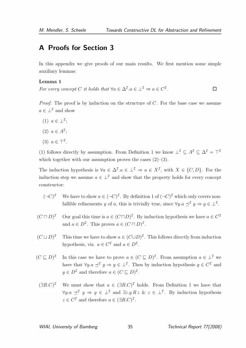
A Proofs for Section 3
In this appendix we give proofs of our main results. We first mention some simple
auxiliary lemmas:
Lemma 1
For every concept C it holds that ∀a ∈ ∆I .a ∈ ⊥I ⇒ a ∈ CI.
Proof. The proof is by induction on the structure of C. For the base case we assume
a ∈ ⊥I and show
(1) a ∈ ⊥I ;
(2) a ∈ AI ;
(3) a ∈ ⊤I .
(1) follows directly by assumption. From Definition 1 we know ⊥I ⊆ AI ⊆ ∆I = ⊤I
which together with our assumption proves the cases (2)–(3).
The induction hypothesis is ∀a ∈ ∆I .a ∈ ⊥I ⇒ a ∈ XI , with X ∈ {C, D}. For the
induction step we assume a ∈ ⊥I and show that the property holds for every concept
constructor:
(¬C)I We have to show a ∈ (¬C)I . By definition 1 of (¬C)I which only covers non-
fallible refinements y of a, this is trivially true, since ∀y.a �I y ⇒ y ∈ ⊥I .
(C ⊓ D)I Our goal this time is a ∈ (C⊓D)I . By induction hypothesis we have a ∈ CI
and a ∈ DI . This proves a ∈ (C ⊓ D)I .
(C ⊔ D)I This time we have to show a ∈ (C⊔D)I . This follows directly from induction
hypothesis, viz. a ∈ CI and a ∈ DI .
(C ⊑ D)I In this case we have to prove a ∈ (C ⊑ D)I . From assumption a ∈ ⊥I we
have that ∀y.a �I y ⇒ y ∈ ⊥I . Then by induction hypothesis y ∈ CI and
y ∈ DI and therefore a ∈ (C ⊑ D)I .
(∃R.C)I We must show that a ∈ (∃R.C)I holds. From Definition 1 we have that
∀y.a �I y ⇒ y ∈ ⊥I and ∃z.y R z & z ∈ ⊥I . By induction hypothesis
z ∈ CI and therefore a ∈ (∃R.C)I .
WIAI, University of Bamberg 35 Technical Report 77(2008)
M. Mendler, S. Scheele Towards Constructive DL for Abstraction and Refinement
(∀R.C)I We have to show that a ∈ (∀R.C)I holds. By Definition 1 we have ∀y.a �I
y ⇒ y ∈ ⊥I and ∀z.y R z ⇒ z ∈ ⊥I , then by induction hypothesis z ∈ CI
which proves our goal.
Lemma 2. Let Θ; Σ; Γ ⊢ Φ; Ψ be an inconsistent sequent, i.e., there exists a closed
tableau for it based on the rules in Fig. 4. Then, the following holds:
1. |Φ ∪⋃
R∈NRΨ(R)| ≥ 1;
2. For every weakening Θ ⊆ Θ′, Σ ⊆ Σ′, Γ ⊆ Γ′, Φ ⊆ Φ′ and Ψ ⊆ Ψ′ the sequent
Θ′; Σ′; Γ′ ⊢ Φ′; Ψ′ is inconsistent, too;
Proof. By induction on the structure of the tableau.
From the first condition 1. expressed in Lem. 2 it can be concluded that all sequents of
the form Θ; Σ; Γ ⊢ ∅; ∅ are necessarily consistent. In fact, such sequents are satisfiable
in any interpretation with a fallible entity.
Theorem 1 [Hilbert Soundness and Completeness]
For every concept C and set of concepts Θ we have Θ; ∅ |= C iff Θ ⊢H C.
Proof. Soundness and completeness follow from soundness and completeness of the
Gentzen tableau system Thm. 2, proven below, if we can show that any deduction in
either system can be translated into the other.
We first show that the tableau system can simulate the Hilbert deductions in the sense
that if Θ ⊢H C then there exists a closed tableau for sequent Θ; ∅; ∅ ⊢ C; ∅. From
this we get soundness of Hilbert Θ ⊢H C ⇒ Θ; ∅ |= C from soundness of Gentzen
(Thm. 2). The simulation amounts to verifying that the Hilbert axioms are derivable
using the rules of Fig. 4 and that the Hilbert rules of Modus Ponens and Necessitation
are derivable or admissible in the tableau system. Tableau derivations of the Hilbert
axioms ∀K and ∃K in the form ∅; ∅; ∅ ⊢ ∀R.(A ⊑ B) ⊑ (∀R.A ⊑ ∀R.B); ∅ and
∅; ∅; ∅ ⊢ (∀R.A ⊓ ∃R.B) ⊑ ∃R.(A ⊓ B); ∅ have been given in Example 7 on page 25.
The other axioms of intuitionistic logic which we list in Fig. 14 are easily constructed,
too.
WIAI, University of Bamberg 36 Technical Report 77(2008)
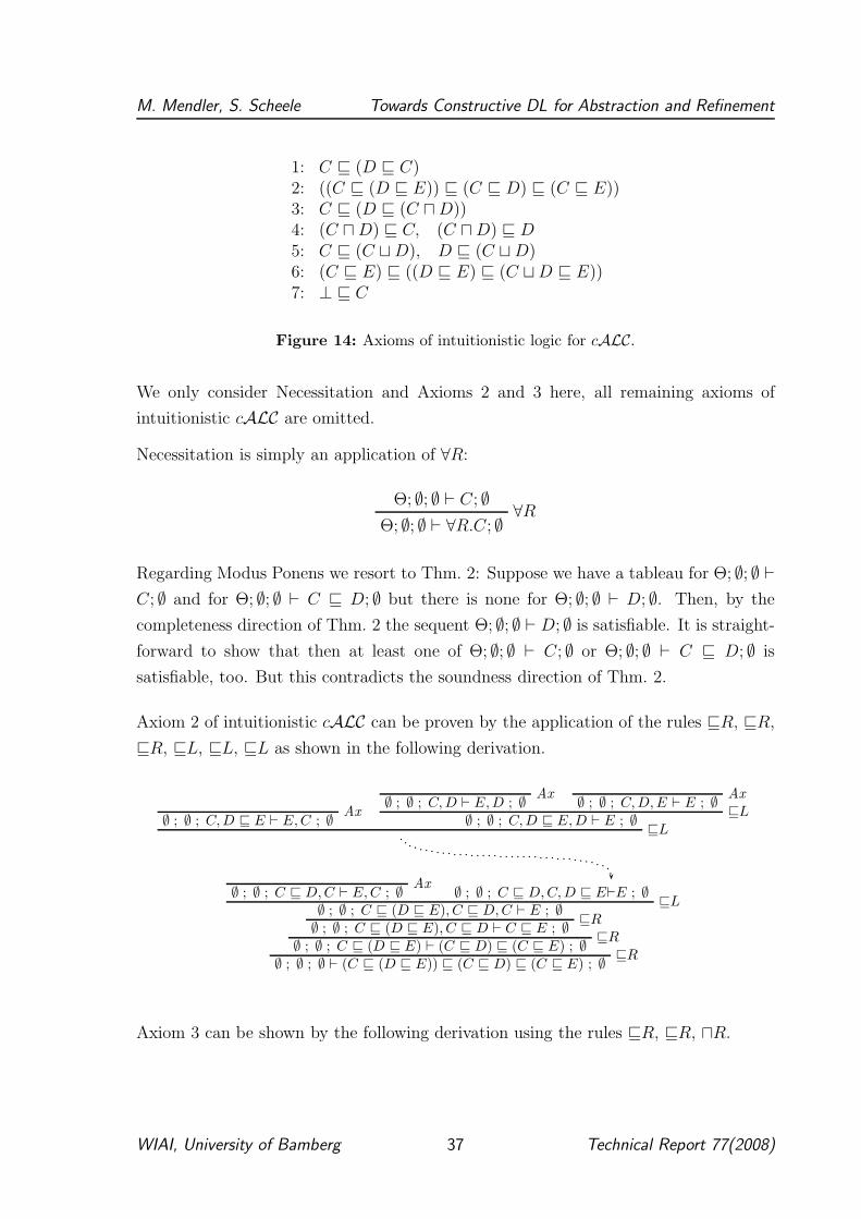
M. Mendler, S. Scheele Towards Constructive DL for Abstraction and Refinement
1: C ⊑ (D ⊑ C)2: ((C ⊑ (D ⊑ E)) ⊑ (C ⊑ D) ⊑ (C ⊑ E))3: C ⊑ (D ⊑ (C ⊓ D))4: (C ⊓ D) ⊑ C, (C ⊓ D) ⊑ D
5: C ⊑ (C ⊔ D), D ⊑ (C ⊔ D)6: (C ⊑ E) ⊑ ((D ⊑ E) ⊑ (C ⊔ D ⊑ E))7: ⊥ ⊑ C
Figure 14: Axioms of intuitionistic logic for cALC.
We only consider Necessitation and Axioms 2 and 3 here, all remaining axioms of
intuitionistic cALC are omitted.
Necessitation is simply an application of ∀R:
Θ; ∅; ∅ ⊢ C; ∅∀R
Θ; ∅; ∅ ⊢ ∀R.C; ∅
Regarding Modus Ponens we resort to Thm. 2: Suppose we have a tableau for Θ; ∅; ∅ ⊢
C; ∅ and for Θ; ∅; ∅ ⊢ C ⊑ D; ∅ but there is none for Θ; ∅; ∅ ⊢ D; ∅. Then, by the
completeness direction of Thm. 2 the sequent Θ; ∅; ∅ ⊢ D; ∅ is satisfiable. It is straight-
forward to show that then at least one of Θ; ∅; ∅ ⊢ C; ∅ or Θ; ∅; ∅ ⊢ C ⊑ D; ∅ is
satisfiable, too. But this contradicts the soundness direction of Thm. 2.
Axiom 2 of intuitionistic cALC can be proven by the application of the rules ⊑R, ⊑R,
⊑R, ⊑L, ⊑L, ⊑L as shown in the following derivation.
Ax∅ ; ∅ ; C, D ⊑ E ⊢ E, C ; ∅
Ax∅ ; ∅ ; C, D ⊢ E, D ; ∅
Ax∅ ; ∅ ; C, D, E ⊢ E ; ∅
⊑L∅ ; ∅ ; C, D ⊑ E, D ⊢ E ; ∅
⊑L
Ax∅ ; ∅ ; C ⊑ D, C ⊢ E, C ; ∅ ∅ ; ∅ ; C ⊑ D, C, D ⊑ E⊢E ; ∅
⊑L∅ ; ∅ ; C ⊑ (D ⊑ E), C ⊑ D, C ⊢ E ; ∅
⊑R∅ ; ∅ ; C ⊑ (D ⊑ E), C ⊑ D ⊢ C ⊑ E ; ∅
⊑R∅ ; ∅ ; C ⊑ (D ⊑ E) ⊢ (C ⊑ D) ⊑ (C ⊑ E) ; ∅
⊑R∅ ; ∅ ; ∅ ⊢ (C ⊑ (D ⊑ E)) ⊑ (C ⊑ D) ⊑ (C ⊑ E) ; ∅
Axiom 3 can be shown by the following derivation using the rules ⊑R, ⊑R, ⊓R.
WIAI, University of Bamberg 37 Technical Report 77(2008)
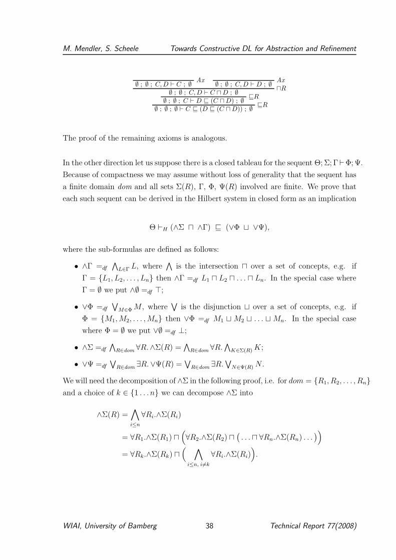
M. Mendler, S. Scheele Towards Constructive DL for Abstraction and Refinement
Ax∅ ; ∅ ; C, D ⊢ C ; ∅
Ax∅ ; ∅ ; C, D ⊢ D ; ∅
⊓R∅ ; ∅ ; C, D ⊢ C ⊓ D ; ∅
⊑R∅ ; ∅ ; C ⊢ D ⊑ (C ⊓ D) ; ∅
⊑R∅ ; ∅ ; ∅ ⊢ C ⊑ (D ⊑ (C ⊓ D)) ; ∅
The proof of the remaining axioms is analogous.
In the other direction let us suppose there is a closed tableau for the sequent Θ; Σ; Γ⊢Φ; Ψ.
Because of compactness we may assume without loss of generality that the sequent has
a finite domain dom and all sets Σ(R), Γ, Φ, Ψ(R) involved are finite. We prove that
each such sequent can be derived in the Hilbert system in closed form as an implication
Θ ⊢H (∧Σ ⊓ ∧Γ) ⊑ (∨Φ ⊔ ∨Ψ),
where the sub-formulas are defined as follows:
• ∧Γ =df
∧
L∈Γ L, where∧
is the intersection ⊓ over a set of concepts, e.g. if
Γ = {L1, L2, . . . , Ln} then ∧Γ =df L1 ⊓ L2 ⊓ . . . ⊓ Ln. In the special case where
Γ = ∅ we put ∧∅ =df ⊤;
• ∨Φ =df
∨
M∈Φ M , where∨
is the disjunction ⊔ over a set of concepts, e.g. if
Φ = {M1, M2, . . . , Mn} then ∨Φ =df M1 ⊔ M2 ⊔ . . . ⊔ Mn. In the special case
where Φ = ∅ we put ∨∅ =df ⊥;
• ∧Σ =df
∧
R∈dom∀R.∧Σ(R) =
∧
R∈dom∀R.
∧
K∈Σ(R) K;
• ∨Ψ =df
∨
R∈dom∃R.∨Ψ(R) =
∨
R∈dom∃R.
∨
N∈Ψ(R) N .
We will need the decomposition of ∧Σ in the following proof, i.e. for dom = {R1, R2, . . . , Rn}
and a choice of k ∈ {1 . . . n} we can decompose ∧Σ into
∧Σ(R) =∧
i≤n
∀Ri.∧Σ(Ri)
= ∀R1.∧Σ(R1) ⊓(
∀R2.∧Σ(R2) ⊓(
. . . ⊓ ∀Rn.∧Σ(Rn) . . .)
)
= ∀Rk.∧Σ(Rk) ⊓(
∧
i≤n, i6=k
∀Ri.∧Σ(Ri))
.
WIAI, University of Bamberg 38 Technical Report 77(2008)
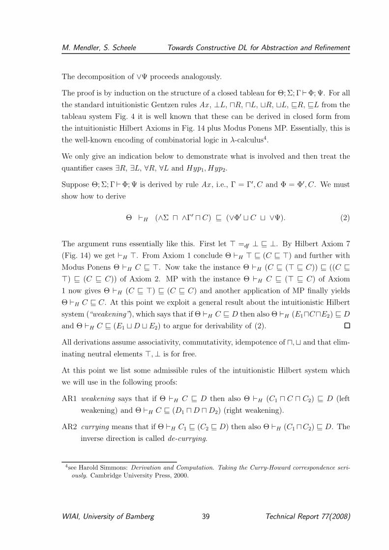
M. Mendler, S. Scheele Towards Constructive DL for Abstraction and Refinement
The decomposition of ∨Ψ proceeds analogously.
The proof is by induction on the structure of a closed tableau for Θ; Σ; Γ⊢Φ; Ψ. For all
the standard intuitionistic Gentzen rules Ax , ⊥L, ⊓R, ⊓L, ⊔R, ⊔L, ⊑R, ⊑L from the
tableau system Fig. 4 it is well known that these can be derived in closed form from
the intuitionistic Hilbert Axioms in Fig. 14 plus Modus Ponens MP. Essentially, this is
the well-known encoding of combinatorial logic in λ-calculus4.
We only give an indication below to demonstrate what is involved and then treat the
quantifier cases ∃R, ∃L, ∀R, ∀L and Hyp1, Hyp2.
Suppose Θ; Σ; Γ⊢Φ; Ψ is derived by rule Ax , i.e., Γ = Γ′, C and Φ = Φ′, C. We must
show how to derive
Θ ⊢H (∧Σ ⊓ ∧Γ′ ⊓ C) ⊑ (∨Φ′ ⊔ C ⊔ ∨Ψ). (2)
The argument runs essentially like this. First let ⊤ =df ⊥ ⊑ ⊥. By Hilbert Axiom 7
(Fig. 14) we get ⊢H ⊤. From Axiom 1 conclude Θ ⊢H ⊤ ⊑ (C ⊑ ⊤) and further with
Modus Ponens Θ ⊢H C ⊑ ⊤. Now take the instance Θ ⊢H (C ⊑ (⊤ ⊑ C)) ⊑ ((C ⊑
⊤) ⊑ (C ⊑ C)) of Axiom 2. MP with the instance Θ ⊢H C ⊑ (⊤ ⊑ C) of Axiom
1 now gives Θ ⊢H (C ⊑ ⊤) ⊑ (C ⊑ C) and another application of MP finally yields
Θ ⊢H C ⊑ C. At this point we exploit a general result about the intuitionistic Hilbert
system (“weakening”), which says that if Θ ⊢H C ⊑ D then also Θ ⊢H (E1⊓C⊓E2) ⊑ D
and Θ ⊢H C ⊑ (E1 ⊔ D ⊔ E2) to argue for derivability of (2).
All derivations assume associativity, commutativity, idempotence of ⊓,⊔ and that elim-
inating neutral elements ⊤,⊥ is for free.
At this point we list some admissible rules of the intuitionistic Hilbert system which
we will use in the following proofs:
AR1 weakening says that if Θ ⊢H C ⊑ D then also Θ ⊢H (C1 ⊓ C ⊓ C2) ⊑ D (left
weakening) and Θ ⊢H C ⊑ (D1 ⊓ D ⊓ D2) (right weakening).
AR2 currying means that if Θ ⊢H C1 ⊑ (C2 ⊑ D) then also Θ ⊢H (C1 ⊓C2) ⊑ D. The
inverse direction is called de-currying.
4see Harold Simmons: Derivation and Computation. Taking the Curry-Howard correspondence seri-
ously. Cambridge University Press, 2000.
WIAI, University of Bamberg 39 Technical Report 77(2008)
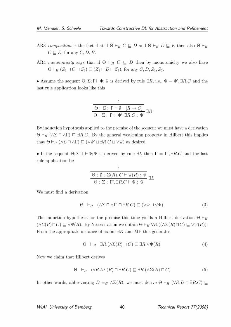
M. Mendler, S. Scheele Towards Constructive DL for Abstraction and Refinement
AR3 composition is the fact that if Θ ⊢H C ⊑ D and Θ ⊢H D ⊑ E then also Θ ⊢H
C ⊑ E, for any C, D, E.
AR4 monotonicity says that if Θ ⊢H C ⊑ D then by monotonicity we also have
Θ ⊢H (Z1 ⊓ C ⊓ Z2) ⊑ (Z1 ⊓ D ⊓ Z2), for any C, D, Z1, Z2.
• Assume the sequent Θ; Σ; Γ⊢Φ; Ψ is derived by rule ∃R, i.e., Φ = Φ′, ∃R.C and the
last rule application looks like this
...
Θ ; Σ ; Γ ⊢ ∅ ; [R 7→ C]∃R
Θ ; Σ ; Γ ⊢ Φ′, ∃R.C ; Ψ
By induction hypothesis applied to the premise of the sequent we must have a derivation
Θ ⊢H (∧Σ ⊓ ∧Γ) ⊑ ∃R.C. By the general weakening property in Hilbert this implies
that Θ ⊢H (∧Σ ⊓ ∧Γ) ⊑ (∨Φ′ ⊔ ∃R.C ⊔ ∨Ψ) as desired.
• If the sequent Θ; Σ; Γ⊢Φ; Ψ is derived by rule ∃L then Γ = Γ′, ∃R.C and the last
rule application be...
Θ ; ∅ ; Σ(R), C ⊢ Ψ(R) ; ∅∃L
Θ ; Σ ; Γ′, ∃R.C ⊢ Φ ; Ψ
We must find a derivation
Θ ⊢H (∧Σ ⊓ ∧Γ′ ⊓ ∃R.C) ⊑ (∨Φ ⊔ ∨Ψ). (3)
The induction hypothesis for the premise this time yields a Hilbert derivation Θ ⊢H
(∧Σ(R)⊓C) ⊑ ∨Ψ(R). By Necessitation we obtain Θ ⊢H ∀R.((∧Σ(R)⊓C) ⊑ ∨Ψ(R)).
From the appropriate instance of axiom ∃K and MP this generates
Θ ⊢H ∃R.(∧Σ(R) ⊓ C) ⊑ ∃R.∨Ψ(R). (4)
Now we claim that Hilbert derives
Θ ⊢H (∀R.∧Σ(R) ⊓ ∃R.C) ⊑ ∃R.(∧Σ(R) ⊓ C) (5)
In other words, abbreviating D =df ∧Σ(R), we must derive Θ ⊢H (∀R.D ⊓ ∃R.C) ⊑
WIAI, University of Bamberg 40 Technical Report 77(2008)
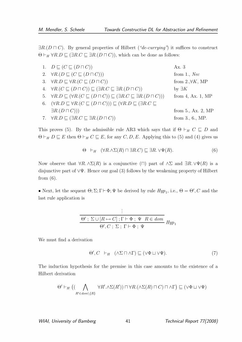
M. Mendler, S. Scheele Towards Constructive DL for Abstraction and Refinement
∃R.(D ⊓ C). By general properties of Hilbert (“de-currying”) it suffices to construct
Θ ⊢H ∀R.D ⊑ (∃R.C ⊑ ∃R.(D ⊓ C)), which can be done as follows:
1. D ⊑ (C ⊑ (D ⊓ C)) Ax. 3
2. ∀R.(D ⊑ (C ⊑ (D ⊓ C))) from 1., Nec
3. ∀R.D ⊑ ∀R.(C ⊑ (D ⊓ C)) from 2.,∀K, MP
4. ∀R.(C ⊑ (D ⊓ C)) ⊑ (∃R.C ⊑ ∃R.(D ⊓ C)) by ∃K
5. ∀R.D ⊑ (∀R.(C ⊑ (D ⊓ C)) ⊑ (∃R.C ⊑ ∃R.(D ⊓ C))) from 4, Ax. 1, MP
6. (∀R.D ⊑ ∀R.(C ⊑ (D ⊓ C))) ⊑ (∀R.D ⊑ (∃R.C ⊑
∃R.(D ⊓ C))) from 5., Ax. 2, MP
7. ∀R.D ⊑ (∃R.C ⊑ ∃R.(D ⊓ C)) from 3., 6., MP.
This proves (5). By the admissible rule AR3 which says that if Θ ⊢H C ⊑ D and
Θ ⊢H D ⊑ E then Θ ⊢H C ⊑ E, for any C, D, E. Applying this to (5) and (4) gives us
Θ ⊢H (∀R.∧Σ(R) ⊓ ∃R.C) ⊑ ∃R.∨Ψ(R). (6)
Now observe that ∀R.∧Σ(R) is a conjunctive (⊓) part of ∧Σ and ∃R.∨Ψ(R) is a
disjunctive part of ∨Ψ. Hence our goal (3) follows by the weakening property of Hilbert
from (6).
• Next, let the sequent Θ; Σ; Γ⊢Φ; Ψ be derived by rule Hyp1, i.e., Θ = Θ′, C and the
last rule application is
...
Θ′ ; Σ ∪ [R 7→ C] ; Γ ⊢ Φ ; Ψ R ∈ domHyp1
Θ′, C ; Σ ; Γ ⊢ Φ ; Ψ
We must find a derivation
Θ′, C ⊢H (∧Σ ⊓ ∧Γ) ⊑ (∨Φ ⊔ ∨Ψ). (7)
The induction hypothesis for the premise in this case amounts to the existence of a
Hilbert derivation
Θ′ ⊢H
(
(∧
R′∈dom\{R}
∀R′.∧Σ(R′)) ⊓ ∀R.(∧Σ(R) ⊓ C) ⊓ ∧Γ)
⊑ (∨Φ ⊔ ∨Ψ)
WIAI, University of Bamberg 41 Technical Report 77(2008)
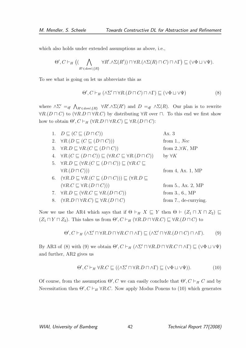
M. Mendler, S. Scheele Towards Constructive DL for Abstraction and Refinement
which also holds under extended assumptions as above, i.e.,
Θ′, C ⊢H
(
(∧
R′∈dom\{R}
∀R′.∧Σ(R′)) ⊓ ∀R.(∧Σ(R) ⊓ C) ⊓ ∧Γ)
⊑ (∨Φ ⊔ ∨Ψ).
To see what is going on let us abbreviate this as
Θ′, C ⊢H (∧Σ′ ⊓ ∀R.(D ⊓ C) ⊓ ∧Γ) ⊑ (∨Φ ⊔ ∨Ψ) (8)
where ∧Σ′ =df
∧
R′∈dom\{R} ∀R′.∧Σ(R′) and D =df ∧Σ(R). Our plan is to rewrite
∀R.(D ⊓ C) to (∀R.D ⊓ ∀R.C) by distributing ∀R over ⊓. To this end we first show
how to obtain Θ′, C ⊢H (∀R.D ⊓ ∀R.C) ⊑ ∀R.(D ⊓ C):
1. D ⊑ (C ⊑ (D ⊓ C)) Ax. 3
2. ∀R.(D ⊑ (C ⊑ (D ⊓ C))) from 1., Nec
3. ∀R.D ⊑ ∀R.(C ⊑ (D ⊓ C)) from 2.,∀K, MP
4. ∀R.(C ⊑ (D ⊓ C)) ⊑ (∀R.C ⊑ ∀R.(D ⊓ C)) by ∀K
5. ∀R.D ⊑ (∀R.(C ⊑ (D ⊓ C)) ⊑ (∀R.C ⊑
∀R.(D ⊓ C))) from 4, Ax. 1, MP
6. (∀R.D ⊑ ∀R.(C ⊑ (D ⊓ C))) ⊑ (∀R.D ⊑
(∀R.C ⊑ ∀R.(D ⊓ C))) from 5., Ax. 2, MP
7. ∀R.D ⊑ (∀R.C ⊑ ∀R.(D ⊓ C)) from 3., 6., MP
8. (∀R.D ⊓ ∀R.C) ⊑ ∀R.(D ⊓ C) from 7., de-currying.
Now we use the AR4 which says that if Θ ⊢H X ⊑ Y then Θ ⊢ (Z1 ⊓ X ⊓ Z2) ⊑
(Z1 ⊓ Y ⊓ Z2). This takes us from Θ′, C ⊢H (∀R.D ⊓ ∀R.C) ⊑ ∀R.(D ⊓ C) to
Θ′, C ⊢H (∧Σ′ ⊓ ∀R.D ⊓ ∀R.C ⊓ ∧Γ) ⊑ (∧Σ′ ⊓ ∀R.(D ⊓ C) ⊓ ∧Γ). (9)
By AR3 of (8) with (9) we obtain Θ′, C ⊢H (∧Σ′ ⊓ ∀R.D ⊓ ∀R.C ⊓ ∧Γ) ⊑ (∨Φ ⊔ ∨Ψ)
and further, AR2 gives us
Θ′, C ⊢H ∀R.C ⊑ ((∧Σ′ ⊓ ∀R.D ⊓ ∧Γ) ⊑ (∨Φ ⊔ ∨Ψ)). (10)
Of course, from the assumption Θ′, C we can easily conclude that Θ′, C ⊢H C and by
Necessitation then Θ′, C ⊢H ∀R.C. Now apply Modus Ponens to (10) which generates
WIAI, University of Bamberg 42 Technical Report 77(2008)
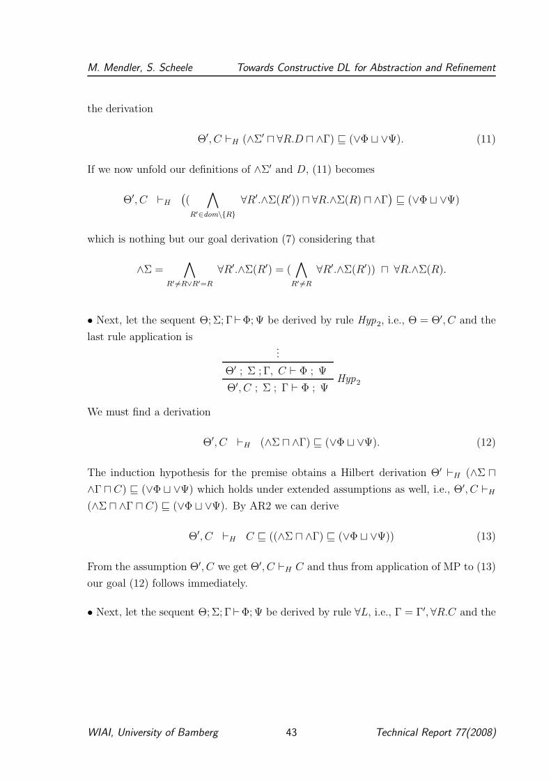
M. Mendler, S. Scheele Towards Constructive DL for Abstraction and Refinement
the derivation
Θ′, C ⊢H (∧Σ′ ⊓ ∀R.D ⊓ ∧Γ) ⊑ (∨Φ ⊔ ∨Ψ). (11)
If we now unfold our definitions of ∧Σ′ and D, (11) becomes
Θ′, C ⊢H
(
(∧
R′∈dom\{R}
∀R′.∧Σ(R′)) ⊓ ∀R.∧Σ(R) ⊓ ∧Γ)
⊑ (∨Φ ⊔ ∨Ψ)
which is nothing but our goal derivation (7) considering that
∧Σ =∧
R′ 6=R∨R′=R
∀R′.∧Σ(R′) = (∧
R′ 6=R
∀R′.∧Σ(R′)) ⊓ ∀R.∧Σ(R).
• Next, let the sequent Θ; Σ; Γ⊢Φ; Ψ be derived by rule Hyp2, i.e., Θ = Θ′, C and the
last rule application is...
Θ′ ; Σ ; Γ, C ⊢ Φ ; ΨHyp2
Θ′, C ; Σ ; Γ ⊢ Φ ; Ψ
We must find a derivation
Θ′, C ⊢H (∧Σ ⊓ ∧Γ) ⊑ (∨Φ ⊔ ∨Ψ). (12)
The induction hypothesis for the premise obtains a Hilbert derivation Θ′ ⊢H (∧Σ ⊓
∧Γ ⊓ C) ⊑ (∨Φ ⊔ ∨Ψ) which holds under extended assumptions as well, i.e., Θ′, C ⊢H
(∧Σ ⊓ ∧Γ ⊓ C) ⊑ (∨Φ ⊔ ∨Ψ). By AR2 we can derive
Θ′, C ⊢H C ⊑ ((∧Σ ⊓ ∧Γ) ⊑ (∨Φ ⊔ ∨Ψ)) (13)
From the assumption Θ′, C we get Θ′, C ⊢H C and thus from application of MP to (13)
our goal (12) follows immediately.
• Next, let the sequent Θ; Σ; Γ⊢Φ; Ψ be derived by rule ∀L, i.e., Γ = Γ′, ∀R.C and the
WIAI, University of Bamberg 43 Technical Report 77(2008)
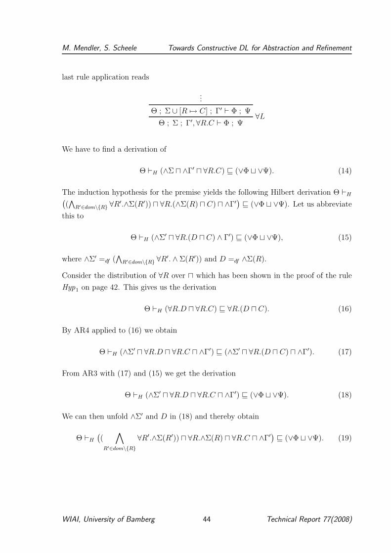
M. Mendler, S. Scheele Towards Constructive DL for Abstraction and Refinement
last rule application reads
...
Θ ; Σ ∪ [R 7→ C] ; Γ′ ⊢ Φ ; Ψ∀L
Θ ; Σ ; Γ′, ∀R.C ⊢ Φ ; Ψ
We have to find a derivation of
Θ ⊢H (∧Σ ⊓ ∧Γ′ ⊓ ∀R.C) ⊑ (∨Φ ⊔ ∨Ψ). (14)
The induction hypothesis for the premise yields the following Hilbert derivation Θ ⊢H(
(∧
R′∈dom\{R} ∀R′.∧Σ(R′)) ⊓ ∀R.(∧Σ(R) ⊓ C) ⊓ ∧Γ′)
⊑ (∨Φ ⊔ ∨Ψ). Let us abbreviate
this to
Θ ⊢H (∧Σ′ ⊓ ∀R.(D ⊓ C) ∧ Γ′) ⊑ (∨Φ ⊔ ∨Ψ), (15)
where ∧Σ′ =df (∧
R′∈dom\{R} ∀R′. ∧ Σ(R′)) and D =df ∧Σ(R).
Consider the distribution of ∀R over ⊓ which has been shown in the proof of the rule
Hyp1 on page 42. This gives us the derivation
Θ ⊢H (∀R.D ⊓ ∀R.C) ⊑ ∀R.(D ⊓ C). (16)
By AR4 applied to (16) we obtain
Θ ⊢H (∧Σ′ ⊓ ∀R.D ⊓ ∀R.C ⊓ ∧Γ′) ⊑ (∧Σ′ ⊓ ∀R.(D ⊓ C) ⊓ ∧Γ′). (17)
From AR3 with (17) and (15) we get the derivation
Θ ⊢H (∧Σ′ ⊓ ∀R.D ⊓ ∀R.C ⊓ ∧Γ′) ⊑ (∨Φ ⊔ ∨Ψ). (18)
We can then unfold ∧Σ′ and D in (18) and thereby obtain
Θ ⊢H
(
(∧
R′∈dom\{R}
∀R′.∧Σ(R′)) ⊓ ∀R.∧Σ(R) ⊓ ∀R.C ⊓ ∧Γ′)
⊑ (∨Φ ⊔ ∨Ψ). (19)
WIAI, University of Bamberg 44 Technical Report 77(2008)
M. Mendler, S. Scheele Towards Constructive DL for Abstraction and Refinement
Considering that
∧Σ =∧
R′ 6=R∨R′=R
∀R′.∧Σ(R′) =(
∧
R′ 6=R
∀R′.∧Σ(R′))
⊓ ∀R.∧Σ(R)
we obtain from (19) our goal (14) as desired.
• Next, let the sequent Θ; Σ; Γ⊢Φ; Ψ be derived by rule ∀R, i.e., Φ = Φ′, ∀R.C and the
last rule application reads
...
Θ ; ∅ ; Σ(R) ⊢ C ; ∅∀R
Θ ; Σ ; Γ′ ⊢ Φ′, ∀R.C ; Ψ
We have to find a derivation of
Θ ⊢H (∧Σ ⊓ ∧Γ) ⊑ (∨Φ′ ⊔ ∀R.C ⊔ ∨Ψ). (20)
The induction hypothesis for the premise yields this time a Hilbert derivation Θ ⊢H
∧Σ(R) ⊑ C. By Necessitation we obtain Θ ⊢H ∀R.(∧Σ(R) ⊑ C). From the appropriate
instance of the Hilbert axiom ∀K and MP this generates
Θ ⊢H ∀R.∧Σ(R) ⊑ ∀R.C (21)
Left- and right-weakening (AR1) of (21) then gives us
Θ ⊢H
(
(∧
R′∈dom\{R}
∀R′.∧Σ(R′)) ⊓ ∀R.∧Σ(R) ⊓ ∧Γ)
⊑ (∨Φ′ ⊔ ∀R.C ⊔ ∨Ψ) (22)
which by Definition of
∧Σ =∧
R′ 6=R∨R′=R
∀R′.∧Σ(R′) =(
∧
R′ 6=R
∀R′.∧Σ(R′))
⊓ ∀R.∧Σ(R)
gives us Θ ⊢H (∧Σ(R) ⊓ ∧Γ) ⊑ (∨Φ′ ⊔ ∀R.C ⊔ ∨Ψ) which is the goal (20) that was to
be shown.
WIAI, University of Bamberg 45 Technical Report 77(2008)
M. Mendler, S. Scheele Towards Constructive DL for Abstraction and Refinement
Theorem 2 [Tableau Soundness]
Every satisfiable sequent is consistent, i.e., if Θ; Σ; Γ 6|= Φ; Ψ then Θ; Σ; Γ 6⊢ Φ; Ψ.
Proof. For soundness we must show for each derivation rule in Fig. 4 that if the con-
clusion is satisfiable then at least one of the premises of the rule is satisfiable.
In the special case of the axiom Ax without any premise it is trivial to see that this
sequent cannot be satisfied by any interpretation I and entity a ∈ ∆I , since it is
impossible to obtain a pair (I, a) such that I; a |= C and I; a 6|= C. This is equiva-
lent to saying that the conclusion of Ax , namely the sequent Θ; Σ; Γ, C ⊢ Φ, C; Ψ is
unsatisfiable.
The same is true for the axiom ⊥L with conclusion Θ; Σ; Γ,⊥ ⊢ Φ; Ψ. Notice, here it
is crucial that the right-hand side Φ; Ψ is constrained to be non-empty.
The sequent Θ; Σ; Γ,⊥ ⊢ ∅; ∅, for instance, is satisfiable in a fallible entity. Starting
from these axioms it then follows by induction on the size of a tableau that whenever
a sequent Θ; Σ; Γ ⊢ Φ; Ψ is derivable (i.e., not consistent) then it cannot be satisfiable.
To show soundness of ⊔L we assume its conclusion sequent Sc =df Θ; Σ; Γ, C ⊔
D ⊢ Φ; Ψ is satisfiable and then show that one of its premises, namely the sequents
Sp1 =df Θ; Σ; Γ, C ⊢ Φ; Ψ or Sp2 =df Θ; Σ; Γ, D ⊢ Φ; Ψ, is satisfiable as well. If Sc
is satisfiable then by Definition 2 of constructive satisfiability there exists a pair (I, a)
that satisfies the sequent Sc, i.e. I is a model of Θ, I |= Θ, and for all R ∈ dom,
L ∈ Σ(R), M ∈ Γ ∪ {C ⊔ D}, N ∈ Φ and K ∈ Ψ(R):
∀a′. ∀b. (a � a′ & a′ R b) ⇒ I; b |= L; (23)
I; a |= M, in particular I; a |= C ⊔ D; (24)
I; a 6|= N ; (25)
∀b. a R b ⇒ I; b 6|= K; (26)
• We claim that (I, a) satisfies Sp1 or Sp2. By Definition 1 of constructive inter-
pretation and from I; a |= C ⊔ D we see that a is contained in the union of the
interpretation of the concepts C and D, i.e. I; a |= C or I; a |= D. In the first
WIAI, University of Bamberg 46 Technical Report 77(2008)
M. Mendler, S. Scheele Towards Constructive DL for Abstraction and Refinement
case (I, a) satisfies Sp1 using (23–26) and in the second case (I, a) satisfies Sp2.
This proves our premises of Sc, namely Sp1 by I; a |= C and Sp2 by I; a |= D.
• Regarding the conditions ∀a′. ∀b. (a � a′ & a′ R b) ⇒ I; b |= L, for L ∈ Σ(R),
I; a 6|= N , for N ∈ Φ, and ∀b.aRb ⇒ K, for K ∈ Ψ(R), nothing needs to be shown
here, since the set of role mappings that are supposed to be true for all refinements
of a, the set of formulas and the set of role mappings that are supposed to be
false are equal in Sc and Spi, i = 1, 2.
To show the soundness of ⊓R we assume the conclusion of the rule which is namely the
sequent Θ; Σ; Γ ⊢ Φ, C ⊓D; Ψ is satisfiable and show that one of its premises, namely
the sequents Sp1 =df Θ; Σ; Γ ⊢ Φ, C; Ψ or Sp2 =df Θ; Σ; Γ ⊢ Φ, D; Ψ, is satisfiable
as well. If Sc is satisfiable then by Definition 2 there exists a pair (I, a) with I being
a model of Θ, I |= Θ, and for all R ∈ dom, L ∈ Σ(R), M ∈ Γ, N ∈ Φ ∪ {C ⊓ D} and
K ∈ Ψ(R):
∀a′. ∀b. (a � a′ & a′ R b) ⇒ I; b |= L; (27)
I; a |= M ; (28)
I; a 6|= N, in particular I; a 6|= C ⊓ D; (29)
∀b. a R b ⇒ I; b 6|= K; (30)
We only have to treat the condition I; a 6|= N , for N ∈ Φ ∪ {C} or N ∈ Φ ∪ {D}. The
case I; a 6|= N , for N ∈ Φ follows by assumption (29) since the set Φ is equal in Sc
and Spi, i = 1, 2. Furthermore by Definition 1 of constructive interpretation and from
I; a 6|= C ⊓ D (29) we see that it is false that a is included in C and D, more precisely
by pushing negation inside we get I; a 6|= C or I; a 6|= D. This proves the premises of
Sc, namely Sp1 by I; a 6|= C and Sp2 by I; a 6|= D.
To show soundness of ⊓L we assume the conclusion of the rule which is the se-
quent Sc =df Θ; Σ; Γ, C ⊓ D ⊢ Φ; Ψ is satisfiable and show that its premise
Sp =df Θ; Σ; Γ, C, D ⊢ Φ; Ψ, is satisfiable as well.
If Sc is satisfiable then by Definition 2 of constructive satisfiability there exists a pair
(I, a) that satisfies the sequent Sc, i.e. I is a model of Θ, I |= Θ, and for all R ∈ dom,
WIAI, University of Bamberg 47 Technical Report 77(2008)
M. Mendler, S. Scheele Towards Constructive DL for Abstraction and Refinement
L ∈ Σ(R), M ∈ Γ ∪ {C ⊓ D}, N ∈ Φ and K ∈ Ψ(R):
∀a′. ∀b. (a � a′ & a′ R b) ⇒ I; b |= L; (31)
I; a |= M, in particular I; a |= C ⊓ D; (32)
I; a 6|= N ; (33)
∀b. a R b ⇒ I; b 6|= K; (34)
We only analyse the condition I; a |= M , for M ∈ Γ ∪ {C ⊓ D}. The case I; a |= M ,
for M ∈ Γ follows from (32) and due to the fact that the set Γ is equal in Sc and Sp.
The second case I; a |= C ⊓ D is then used as follows. By Definition 1 of constructive
interpretation and from I; a |= C ⊓ D we get that a is included in the intersection of
the interpretations of C and D, i.e. I; a |= C and I; a |= D. This immediately proves
the premise Sp.
To show soundness of ⊔R we assume the conclusion of the rule Sc =df Θ; Σ; Γ ⊢
Φ, C ⊔ D; Ψ is satisfiable and show that its premise Sp =df Θ; Σ; Γ ⊢ Φ, C, D; Ψ, is
satisfiable as well. If Sc is satisfiable then by Definition 2 of constructive satisfiability
there exists a pair (I, a) that satisfies the sequent Sc, i.e. I is a model of Θ, I |= Θ,
and for all R ∈ dom, L ∈ Σ(R), M ∈ Γ, N ∈ Φ ∪ {C ⊔ D} and K ∈ Ψ(R):
∀a′. ∀b. (a � a′ & a′ R b) ⇒ I; b |= L; (35)
I; a |= M ; (36)
I; a 6|= N, in particular I; a 6|= C ⊔ D; (37)
∀b. a R b ⇒ I; b 6|= K; (38)
We only have to treat the condition I; a 6|= N , for N ∈ Φ∪{C⊔D}. The case I; a 6|= N ,
for N ∈ Φ follows since the set Φ is equal in Sc and Sp. By Definition 1 of constructive
interpretation and from I; a 6|= C ⊔ D we conclude that I; a 6|= C and I; a 6|= D and
therefore obtain I; a 6|= H , with H ∈ {C, D}. This proves the premise Sp.
WIAI, University of Bamberg 48 Technical Report 77(2008)
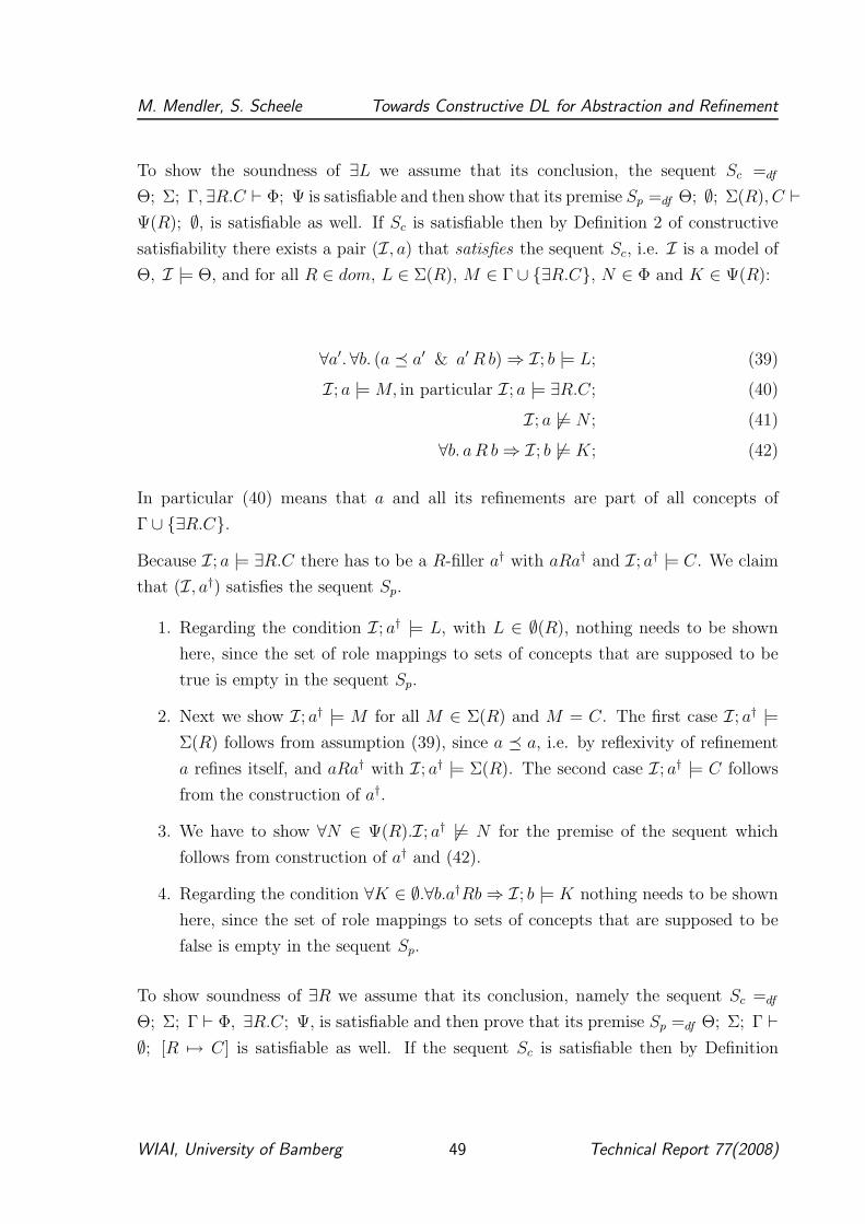
M. Mendler, S. Scheele Towards Constructive DL for Abstraction and Refinement
To show the soundness of ∃L we assume that its conclusion, the sequent Sc =df
Θ; Σ; Γ, ∃R.C ⊢ Φ; Ψ is satisfiable and then show that its premise Sp =df Θ; ∅; Σ(R), C ⊢
Ψ(R); ∅, is satisfiable as well. If Sc is satisfiable then by Definition 2 of constructive
satisfiability there exists a pair (I, a) that satisfies the sequent Sc, i.e. I is a model of
Θ, I |= Θ, and for all R ∈ dom, L ∈ Σ(R), M ∈ Γ ∪ {∃R.C}, N ∈ Φ and K ∈ Ψ(R):
∀a′. ∀b. (a � a′ & a′ R b) ⇒ I; b |= L; (39)
I; a |= M, in particular I; a |= ∃R.C; (40)
I; a 6|= N ; (41)
∀b. a R b ⇒ I; b 6|= K; (42)
In particular (40) means that a and all its refinements are part of all concepts of
Γ ∪ {∃R.C}.
Because I; a |= ∃R.C there has to be a R-filler a† with aRa† and I; a† |= C. We claim
that (I, a†) satisfies the sequent Sp.
1. Regarding the condition I; a† |= L, with L ∈ ∅(R), nothing needs to be shown
here, since the set of role mappings to sets of concepts that are supposed to be
true is empty in the sequent Sp.
2. Next we show I; a† |= M for all M ∈ Σ(R) and M = C. The first case I; a† |=
Σ(R) follows from assumption (39), since a � a, i.e. by reflexivity of refinement
a refines itself, and aRa† with I; a† |= Σ(R). The second case I; a† |= C follows
from the construction of a†.
3. We have to show ∀N ∈ Ψ(R).I; a† 6|= N for the premise of the sequent which
follows from construction of a† and (42).
4. Regarding the condition ∀K ∈ ∅.∀b.a†Rb ⇒ I; b |= K nothing needs to be shown
here, since the set of role mappings to sets of concepts that are supposed to be
false is empty in the sequent Sp.
To show soundness of ∃R we assume that its conclusion, namely the sequent Sc =df
Θ; Σ; Γ ⊢ Φ, ∃R.C; Ψ, is satisfiable and then prove that its premise Sp =df Θ; Σ; Γ ⊢
∅; [R 7→ C] is satisfiable as well. If the sequent Sc is satisfiable then by Definition
WIAI, University of Bamberg 49 Technical Report 77(2008)
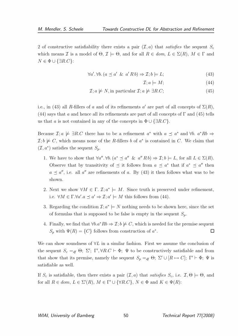
M. Mendler, S. Scheele Towards Constructive DL for Abstraction and Refinement
2 of constructive satisfiability there exists a pair (I, a) that satisfies the sequent Sc
which means I is a model of Θ, I |= Θ, and for all R ∈ dom, L ∈ Σ(R), M ∈ Γ and
N ∈ Φ ∪ {∃R.C}:
∀a′. ∀b. (a � a′ & a′ R b) ⇒ I; b |= L; (43)
I; a |= M ; (44)
I; a 6|= N, in particular I; a 6|= ∃R.C; (45)
i.e., in (43) all R-fillers of a and of its refinements a′ are part of all concepts of Σ(R),
(44) says that a and hence all its refinements are part of all concepts of Γ and (45) tells
us that a is not contained in any of the concepts in Φ ∪ {∃R.C}.
Because I; a 6|= ∃R.C there has to be a refinement a∗ with a � a∗ and ∀b. a∗Rb ⇒
I; b 6|= C, which means none of the R-fillers b of a∗ is contained in C. We claim that
(I, a∗) satisfies the sequent Sp.
1. We have to show that ∀a′′. ∀b. (a∗ � a′′ & a′′ R b) ⇒ I; b |= L, for all L ∈ Σ(R).
Observe that by transitivity of � it follows from a � a∗ that if a∗ � a′′ then
a � a′′, i.e. all a′′ are refinements of a. By (43) it then follows what was to be
shown.
2. Next we show ∀M ∈ Γ. I; a∗ |= M . Since truth is preserved under refinement,
i.e. ∀M ∈ Γ.∀a′.a � a′ ⇒ I; a′ |= M this follows from (44).
3. Regarding the condition I; a∗ |= N nothing needs to be shown here, since the set
of formulas that is supposed to be false is empty in the sequent Sp.
4. Finally, we find that ∀b.a∗Rb ⇒ I; b 6|= C, which is needed for the premise sequent
Sp with Ψ(R) = {C} follows from construction of a∗.
We can show soundness of ∀L in a similar fashion. First we assume the conclusion of
the sequent Sc =df Θ; Σ′; Γ′, ∀R.C ⊢ Φ; Ψ to be constructively satisfiable and from
that show that its premise, namely the sequent Sp =df Θ; Σ′ ∪ [R 7→ C]; Γ′ ⊢ Φ; Ψ is
satisfiable as well.
If Sc is satisfiable, then there exists a pair (I, a) that satisfies Sc, i.e. I, Θ |= Θ, and
for all R ∈ dom, L ∈ Σ′(R), M ∈ Γ′ ∪ {∀R.C}, N ∈ Φ and K ∈ Ψ(R):
WIAI, University of Bamberg 50 Technical Report 77(2008)
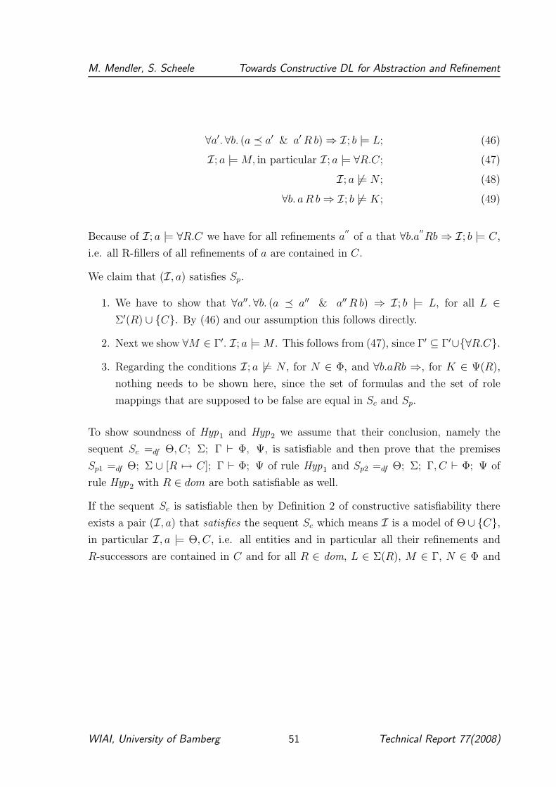
M. Mendler, S. Scheele Towards Constructive DL for Abstraction and Refinement
∀a′. ∀b. (a � a′ & a′ R b) ⇒ I; b |= L; (46)
I; a |= M, in particular I; a |= ∀R.C; (47)
I; a 6|= N ; (48)
∀b. a R b ⇒ I; b 6|= K; (49)
Because of I; a |= ∀R.C we have for all refinements a′′
of a that ∀b.a′′
Rb ⇒ I; b |= C,
i.e. all R-fillers of all refinements of a are contained in C.
We claim that (I, a) satisfies Sp.
1. We have to show that ∀a′′. ∀b. (a � a′′ & a′′ R b) ⇒ I; b |= L, for all L ∈
Σ′(R) ∪ {C}. By (46) and our assumption this follows directly.
2. Next we show ∀M ∈ Γ′. I; a |= M . This follows from (47), since Γ′ ⊆ Γ′∪{∀R.C}.
3. Regarding the conditions I; a 6|= N , for N ∈ Φ, and ∀b.aRb ⇒, for K ∈ Ψ(R),
nothing needs to be shown here, since the set of formulas and the set of role
mappings that are supposed to be false are equal in Sc and Sp.
To show soundness of Hyp1 and Hyp2 we assume that their conclusion, namely the
sequent Sc =df Θ, C; Σ; Γ ⊢ Φ, Ψ, is satisfiable and then prove that the premises
Sp1 =df Θ; Σ ∪ [R 7→ C]; Γ ⊢ Φ; Ψ of rule Hyp1 and Sp2 =df Θ; Σ; Γ, C ⊢ Φ; Ψ of
rule Hyp2 with R ∈ dom are both satisfiable as well.
If the sequent Sc is satisfiable then by Definition 2 of constructive satisfiability there
exists a pair (I, a) that satisfies the sequent Sc which means I is a model of Θ ∪ {C},
in particular I, a |= Θ, C, i.e. all entities and in particular all their refinements and
R-successors are contained in C and for all R ∈ dom, L ∈ Σ(R), M ∈ Γ, N ∈ Φ and
WIAI, University of Bamberg 51 Technical Report 77(2008)
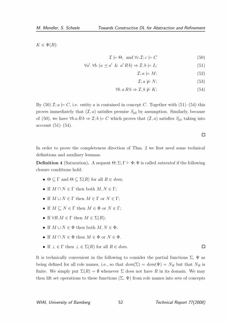
M. Mendler, S. Scheele Towards Constructive DL for Abstraction and Refinement
K ∈ Ψ(R):
I |= Θ, and ∀c.I; c |= C (50)
∀a′. ∀b. (a � a′ & a′ R b) ⇒ I; b |= L; (51)
I; a |= M ; (52)
I; a 6|= N ; (53)
∀b. a R b ⇒ I; b 6|= K; (54)
By (50) I; a |= C, i.e. entity a is contained in concept C. Together with (51)–(54) this
proves immediately that (I, a) satisfies premise Sp2 by assumption. Similarly, because
of (50), we have ∀b.a R b ⇒ I; b |= C which proves that (I, a) satisfies Sp1 taking into
account (51)–(54).
In order to prove the completeness direction of Thm. 2 we first need some technical
definitions and auxiliary lemmas.
Definition 4 (Saturation). A sequent Θ; Σ; Γ ⊢ Φ; Ψ is called saturated if the following
closure conditions hold:
• Θ ⊆ Γ and Θ ⊆ Σ(R) for all R ∈ dom;
• If M ⊓ N ∈ Γ then both M, N ∈ Γ;
• If M ⊔ N ∈ Γ then M ∈ Γ or N ∈ Γ;
• If M ⊑ N ∈ Γ then M ∈ Φ or N ∈ Γ;
• If ∀R.M ∈ Γ then M ∈ Σ(R);
• If M ⊔ N ∈ Φ then both M, N ∈ Φ;
• If M ⊓ N ∈ Φ then M ∈ Φ or N ∈ Φ.
• If ⊥ ∈ Γ then ⊥ ∈ Σ(R) for all R ∈ dom.
It is technically convenient in the following to consider the partial functions Σ, Ψ as
being defined for all role names, i.e., so that dom(Σ) = dom(Ψ) = NR but that NR is
finite. We simply put Σ(R) = ∅ whenever Σ does not have R in its domain. We may
then lift set operations to these functions (Σ, Ψ) from role names into sets of concepts
WIAI, University of Bamberg 52 Technical Report 77(2008)
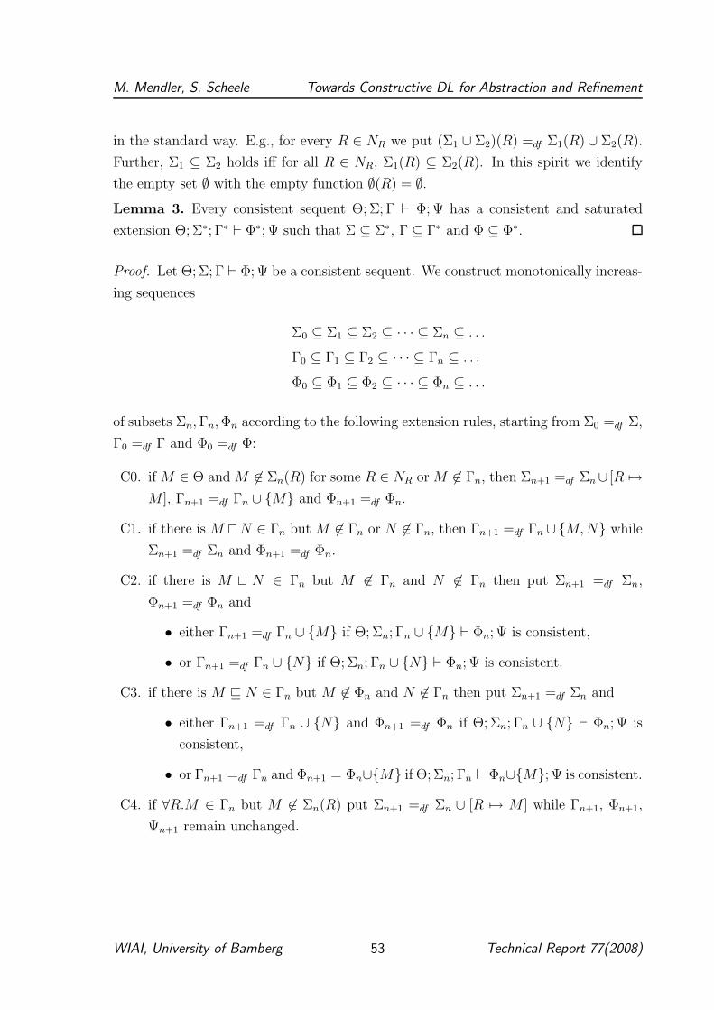
M. Mendler, S. Scheele Towards Constructive DL for Abstraction and Refinement
in the standard way. E.g., for every R ∈ NR we put (Σ1 ∪ Σ2)(R) =df Σ1(R) ∪ Σ2(R).
Further, Σ1 ⊆ Σ2 holds iff for all R ∈ NR, Σ1(R) ⊆ Σ2(R). In this spirit we identify
the empty set ∅ with the empty function ∅(R) = ∅.
Lemma 3. Every consistent sequent Θ; Σ; Γ ⊢ Φ; Ψ has a consistent and saturated
extension Θ; Σ∗; Γ∗ ⊢ Φ∗; Ψ such that Σ ⊆ Σ∗, Γ ⊆ Γ∗ and Φ ⊆ Φ∗.
Proof. Let Θ; Σ; Γ ⊢ Φ; Ψ be a consistent sequent. We construct monotonically increas-
ing sequences
Σ0 ⊆ Σ1 ⊆ Σ2 ⊆ · · · ⊆ Σn ⊆ . . .
Γ0 ⊆ Γ1 ⊆ Γ2 ⊆ · · · ⊆ Γn ⊆ . . .
Φ0 ⊆ Φ1 ⊆ Φ2 ⊆ · · · ⊆ Φn ⊆ . . .
of subsets Σn, Γn, Φn according to the following extension rules, starting from Σ0 =df Σ,
Γ0 =df Γ and Φ0 =df Φ:
C0. if M ∈ Θ and M 6∈ Σn(R) for some R ∈ NR or M 6∈ Γn, then Σn+1 =df Σn∪ [R 7→
M ], Γn+1 =df Γn ∪ {M} and Φn+1 =df Φn.
C1. if there is M ⊓N ∈ Γn but M 6∈ Γn or N 6∈ Γn, then Γn+1 =df Γn ∪ {M, N} while
Σn+1 =df Σn and Φn+1 =df Φn.
C2. if there is M ⊔ N ∈ Γn but M 6∈ Γn and N 6∈ Γn then put Σn+1 =df Σn,
Φn+1 =df Φn and
• either Γn+1 =df Γn ∪ {M} if Θ; Σn; Γn ∪ {M} ⊢ Φn; Ψ is consistent,
• or Γn+1 =df Γn ∪ {N} if Θ; Σn; Γn ∪ {N} ⊢ Φn; Ψ is consistent.
C3. if there is M ⊑ N ∈ Γn but M 6∈ Φn and N 6∈ Γn then put Σn+1 =df Σn and
• either Γn+1 =df Γn ∪ {N} and Φn+1 =df Φn if Θ; Σn; Γn ∪ {N} ⊢ Φn; Ψ is
consistent,
• or Γn+1 =df Γn and Φn+1 = Φn∪{M} if Θ; Σn; Γn ⊢ Φn∪{M}; Ψ is consistent.
C4. if ∀R.M ∈ Γn but M 6∈ Σn(R) put Σn+1 =df Σn ∪ [R 7→ M ] while Γn+1, Φn+1,
Ψn+1 remain unchanged.
WIAI, University of Bamberg 53 Technical Report 77(2008)
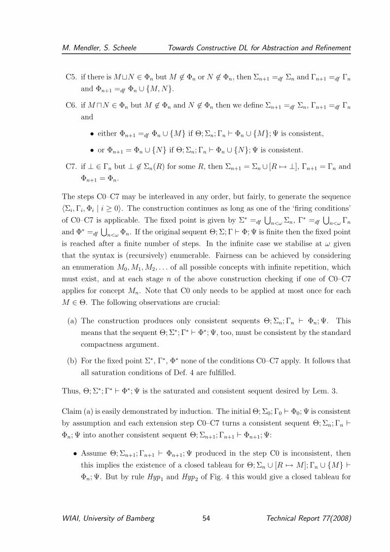
M. Mendler, S. Scheele Towards Constructive DL for Abstraction and Refinement
C5. if there is M⊔N ∈ Φn but M 6∈ Φn or N 6∈ Φn, then Σn+1 =df Σn and Γn+1 =df Γn
and Φn+1 =df Φn ∪ {M, N}.
C6. if M ⊓N ∈ Φn but M 6∈ Φn and N 6∈ Φn then we define Σn+1 =df Σn, Γn+1 =df Γn
and
• either Φn+1 =df Φn ∪ {M} if Θ; Σn; Γn ⊢ Φn ∪ {M}; Ψ is consistent,
• or Φn+1 = Φn ∪ {N} if Θ; Σn; Γn ⊢ Φn ∪ {N}; Ψ is consistent.
C7. if ⊥ ∈ Γn but ⊥ 6∈ Σn(R) for some R, then Σn+1 = Σn ∪ [R 7→ ⊥], Γn+1 = Γn and
Φn+1 = Φn.
The steps C0–C7 may be interleaved in any order, but fairly, to generate the sequence
〈Σi, Γi, Φi | i ≥ 0〉. The construction continues as long as one of the ‘firing conditions’
of C0–C7 is applicable. The fixed point is given by Σ∗ =df
⋃
n<ω Σn, Γ∗ =df
⋃
n<ω Γn
and Φ∗ =df
⋃
n<ω Φn. If the original sequent Θ; Σ; Γ ⊢ Φ; Ψ is finite then the fixed point
is reached after a finite number of steps. In the infinite case we stabilise at ω given
that the syntax is (recursively) enumerable. Fairness can be achieved by considering
an enumeration M0, M1, M2, . . . of all possible concepts with infinite repetition, which
must exist, and at each stage n of the above construction checking if one of C0–C7
applies for concept Mn. Note that C0 only needs to be applied at most once for each
M ∈ Θ. The following observations are crucial:
(a) The construction produces only consistent sequents Θ; Σn; Γn ⊢ Φn; Ψ. This
means that the sequent Θ; Σ∗; Γ∗ ⊢ Φ∗; Ψ, too, must be consistent by the standard
compactness argument.
(b) For the fixed point Σ∗, Γ∗, Φ∗ none of the conditions C0–C7 apply. It follows that
all saturation conditions of Def. 4 are fulfilled.
Thus, Θ; Σ∗; Γ∗ ⊢ Φ∗; Ψ is the saturated and consistent sequent desired by Lem. 3.
Claim (a) is easily demonstrated by induction. The initial Θ; Σ0; Γ0 ⊢ Φ0; Ψ is consistent
by assumption and each extension step C0–C7 turns a consistent sequent Θ; Σn; Γn ⊢
Φn; Ψ into another consistent sequent Θ; Σn+1; Γn+1 ⊢ Φn+1; Ψ:
• Assume Θ; Σn+1; Γn+1 ⊢ Φn+1; Ψ produced in the step C0 is inconsistent, then
this implies the existence of a closed tableau for Θ; Σn ∪ [R 7→ M ]; Γn ∪ {M} ⊢
Φn; Ψ. But by rule Hyp1 and Hyp2 of Fig. 4 this would give a closed tableau for
WIAI, University of Bamberg 54 Technical Report 77(2008)
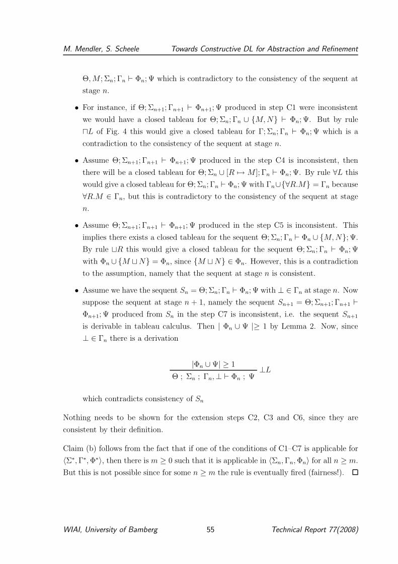
M. Mendler, S. Scheele Towards Constructive DL for Abstraction and Refinement
Θ, M ; Σn; Γn ⊢ Φn; Ψ which is contradictory to the consistency of the sequent at
stage n.
• For instance, if Θ; Σn+1; Γn+1 ⊢ Φn+1; Ψ produced in step C1 were inconsistent
we would have a closed tableau for Θ; Σn; Γn ∪ {M, N} ⊢ Φn; Ψ. But by rule
⊓L of Fig. 4 this would give a closed tableau for Γ; Σn; Γn ⊢ Φn; Ψ which is a
contradiction to the consistency of the sequent at stage n.
• Assume Θ; Σn+1; Γn+1 ⊢ Φn+1; Ψ produced in the step C4 is inconsistent, then
there will be a closed tableau for Θ; Σn ∪ [R 7→ M ]; Γn ⊢ Φn; Ψ. By rule ∀L this
would give a closed tableau for Θ; Σn; Γn ⊢ Φn; Ψ with Γn∪{∀R.M} = Γn because
∀R.M ∈ Γn, but this is contradictory to the consistency of the sequent at stage
n.
• Assume Θ; Σn+1; Γn+1 ⊢ Φn+1; Ψ produced in the step C5 is inconsistent. This
implies there exists a closed tableau for the sequent Θ; Σn; Γn ⊢ Φn ∪ {M, N}; Ψ.
By rule ⊔R this would give a closed tableau for the sequent Θ; Σn; Γn ⊢ Φn; Ψ
with Φn ∪ {M ⊔N} = Φn, since {M ⊔N} ∈ Φn. However, this is a contradiction
to the assumption, namely that the sequent at stage n is consistent.
• Assume we have the sequent Sn = Θ; Σn; Γn ⊢ Φn; Ψ with ⊥ ∈ Γn at stage n. Now
suppose the sequent at stage n + 1, namely the sequent Sn+1 = Θ; Σn+1; Γn+1 ⊢
Φn+1; Ψ produced from Sn in the step C7 is inconsistent, i.e. the sequent Sn+1
is derivable in tableau calculus. Then | Φn ∪ Ψ |≥ 1 by Lemma 2. Now, since
⊥ ∈ Γn there is a derivation
|Φn ∪ Ψ| ≥ 1⊥L
Θ ; Σn ; Γn,⊥ ⊢ Φn ; Ψ
which contradicts consistency of Sn
Nothing needs to be shown for the extension steps C2, C3 and C6, since they are
consistent by their definition.
Claim (b) follows from the fact that if one of the conditions of C1–C7 is applicable for
〈Σ∗, Γ∗, Φ∗〉, then there is m ≥ 0 such that it is applicable in 〈Σn, Γn, Φn〉 for all n ≥ m.
But this is not possible since for some n ≥ m the rule is eventually fired (fairness!).
WIAI, University of Bamberg 55 Technical Report 77(2008)
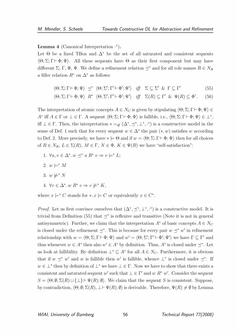
M. Mendler, S. Scheele Towards Constructive DL for Abstraction and Refinement
Lemma 4 (Canonical Interpretation ·∗).
Let Θ be a fixed TBox and ∆∗ be the set of all saturated and consistent sequents
〈Θ; Σ; Γ⊢Φ; Ψ〉. All these sequents have Θ as their first component but may have
different Σ, Γ, Φ, Ψ. We define a refinement relation �∗ and for all role names R ∈ NR
a filler relation R∗ on ∆∗ as follows:
〈Θ; Σ; Γ⊢Φ; Ψ〉 �∗ 〈Θ; Σ′; Γ′ ⊢Φ′; Ψ′〉 iff Σ ⊆ Σ′ & Γ ⊆ Γ′ (55)
〈Θ; Σ; Γ⊢Φ; Ψ〉 R∗ 〈Θ; Σ′; Γ′ ⊢Φ′; Ψ′〉 iff Σ(R) ⊆ Γ′ & Ψ(R) ⊆ Φ′. (56)
The interpretation of atomic concepts A ∈ NC is given by stipulating 〈Θ; Σ; Γ⊢Φ; Ψ〉 ∈
A∗ iff A ∈ Γ or ⊥ ∈ Γ. A sequent 〈Θ; Σ; Γ⊢Φ; Ψ〉 is fallible, i.e., 〈Θ; Σ; Γ⊢Φ; Ψ〉 ∈ ⊥∗,
iff ⊥ ∈ Γ. Then, the interpretation ∗ =df (∆∗,�∗,⊥∗, ·∗) is a constructive model in the
sense of Def. 1 such that for every sequent w ∈ ∆∗ the pair (∗, w) satisfies w according
to Def. 2. More precisely, we have ∗ |= Θ and if w = 〈Θ; Σ; Γ⊢Φ; Ψ〉 then for all choices
of R ∈ NR, L ∈ Σ(R), M ∈ Γ, N ∈ Φ, K ∈ Ψ(R) we have “self-satisfaction”:
1. ∀u, v ∈ ∆∗. w �∗ u R∗ v ⇒ v |=∗ L;
2. w |=∗ M
3. w 6|=∗ N
4. ∀v ∈ ∆∗. w R∗ v ⇒ v 6|=∗ K,
where x |=∗ C stands for ∗, x |= C or equivalently x ∈ C∗.
Proof. Let us first convince ourselves that (∆∗,�∗,⊥∗, ·∗) is a constructive model. It is
trivial from Definition (55) that �∗ is reflexive and transitive (Note it is not in general
antisymmetric). Further, we claim that the interpretation A∗ of basic concepts A ∈ NC
is closed under the refinement �∗. This is because for every pair w �∗ w′ in refinement
relationship with w = 〈Θ; Σ; Γ⊢Φ; Ψ〉 and w′ = 〈Θ; Σ′; Γ′ ⊢Φ′; Ψ′〉 we have Γ ⊆ Γ′ and
thus whenever w ∈ A∗ then also w′ ∈ A∗ by definition. Thus, A∗ is closed under �∗. Let
us look at fallibility. By definition ⊥∗ ⊆ A∗ for all A ∈ NC . Furthermore, it is obvious
that if w �∗ w′ and w is fallible then w′ is fallible, whence ⊥∗ is closed under �∗. If
w ∈ ⊥∗ then by definition of ⊥∗ we have ⊥ ∈ Γ. Now we have to show that there exists a
consistent and saturated sequent w′ such that ⊥ ∈ Γ′ and w R∗ w′. Consider the sequent
S = 〈Θ; ∅; Σ(R)∪{⊥}⊢Ψ(R); ∅〉. We claim that the sequent S is consistent. Suppose,
by contradiction, 〈Θ; ∅; Σ(R),⊥⊢Ψ(R); ∅〉 is derivable. Therefore, Ψ(R) 6= ∅ by Lemma
WIAI, University of Bamberg 56 Technical Report 77(2008)
M. Mendler, S. Scheele Towards Constructive DL for Abstraction and Refinement
2. This contradicts the assumption that 〈Θ; Σ; Γ⊢Φ; Ψ〉 is consistent (by rule ⊥L). By
Lemma 3 there exists a consistent saturated extension S∗ = 〈Θ; Σ∗; Γ∗ ⊢Φ∗; Ψ∗〉 of
〈Θ; ∅; Σ(R),⊥⊢Ψ(R); ∅〉 so that Σ(R)∪ {⊥} ⊆ Γ∗ and Ψ(R) ⊆ Φ∗. Therefore S R∗ S∗
and S∗ ∈ ⊥∗.
We have to show that for a consistent and saturated sequent S with S ∈ ⊥∗, all
R-successors S ′ of S are in ⊥∗. Consider the consistent and saturated sequent S =
〈Θ; Σ; Γ⊢Φ; Ψ〉 with S ∈ ⊥∗. For S we have ⊥ ∈ Γ and by Lemma 3 we know that
⊥ ∈ Σ(R) for all R. Let S ′ = 〈Θ; Σ′; Γ′ ⊢Φ′; Ψ′〉 be an arbitrary R-successor of S.
This means by (56) that ⊥ ∈ Σ(R) ⊆ Γ′ so that S ′ ∈ ⊥∗. Since S ′ was arbitrary all
R-successors of S are in ⊥∗ as claimed.
Thus, ∗ is a constructive model as claimed. Note that all fallible sequents 〈Θ; Σ; Γ⊢Φ; Ψ〉 ∈
∆∗ must be such that Φ = Ψ = ∅ by consistency, otherwise rule ⊥L would make a closed
tableau. Hence, whenever Φ or Ψ(R) for some R ∈ NC are nonempty we know that
〈Θ; Σ; Γ⊢Φ; Ψ〉 ∈ ∆∗c = ∆∗ \ ⊥∗.
Next we claim that ∗ is a model of Θ, i.e., ∗ |= Θ. This follows from the self-satisfaction
condition 2., proven below, and the fact that for all w′ = 〈Θ′; Σ′; Γ′ ⊢Φ′; Ψ′〉 ∈ ∆∗ we
have Θ′ = Θ ⊆ Γ′ by saturation.
It remains to show self-satisfaction, i.e., the truth conditions 1.–4. We first observe
that 1. and 4. follow directly from 2. and 3., respectively, using the definition of
�∗ and R∗ in the model. Let us deal with 4. first. To this end take any R∗-filler
〈Θ; Σ′; Γ′ ⊢Φ′; Ψ′〉 for 〈Θ; Σ; Γ⊢Φ; Ψ〉 in ∗. By construction of R∗, Ψ(R) ⊆ Φ′, which
means that 〈Θ; Σ′; Γ′ ⊢Φ′; Ψ′〉 6|=∗ K for all K ∈ Ψ∗(R) by 3. Regarding 1. consider the
scenario
〈Θ; Σ; Γ⊢Φ; Ψ〉 �∗ 〈Θ; Σ′; Γ′ ⊢Φ′; Ψ′〉 R∗ 〈Θ; Σ′′; Γ′′ ⊢Φ′′; Ψ′′〉
in the canonical interpretation ∗. Our definitions of �∗ and R∗ make sure that Σ(R) ⊆
Σ′(R) ⊆ Γ′′. Thus, for all L ∈ Σ(R) we get 〈Θ; Σ′′; Γ′′ ⊢Φ′′; Ψ′′〉 |= L by 2.
In the rest of the proof we verify conditions 2. and 3. More precisely, for an arbitrary
concept M we show
M ∈ Γ ⇒ 〈Θ; Σ; Γ⊢Φ; Ψ〉 |=∗ M
M ∈ Φ ⇒ 〈Θ; Σ; Γ⊢Φ; Ψ〉 6|=∗ M,
WIAI, University of Bamberg 57 Technical Report 77(2008)
M. Mendler, S. Scheele Towards Constructive DL for Abstraction and Refinement
simultaneously by induction on M . For atomic concepts A ∈ Γ and ⊥ ∈ Γ the statement
is trivial by definition of |=∗. Similarly, for A ∈ Φ we get 〈Θ; Σ; Γ⊢Φ; Ψ〉 6|=∗ A and for
⊥ ∈ Φ we get 〈Θ; Σ; Γ⊢Φ; Ψ〉 6|=∗ ⊥ since otherwise A,⊥ ∈ Γ by definition of |=∗ and
then rule Ax would contradict consistency of 〈Θ; Σ; Γ⊢Φ; Ψ〉.
• Suppose M⊓N ∈ Γ. Then, by saturation of the sequent 〈Θ; Σ; Γ⊢Φ; Ψ〉 we have both
M, N ∈ Γ which means 〈Θ; Σ; Γ⊢Φ; Ψ〉 |=∗ M and 〈Θ; Σ; Γ⊢Φ; Ψ〉 |=∗ N by induction
hypothesis. This implies 〈Θ; Σ; Γ⊢Φ; Ψ〉 |=∗ M ⊓ N .
• If M ⊓ N ∈ Φ then, by saturation of the sequent 〈Θ; Σ; Γ⊢Φ; Ψ〉 this implies that
M ∈ Φ or N ∈ Φ and thus 〈Θ; Σ; Γ⊢Φ; Ψ〉 6|=∗ M or 〈Θ; Σ; Γ⊢Φ; Ψ〉 6|=∗ N by induction
hypothesis from which we get 〈Θ; Σ; Γ⊢Φ; Ψ〉 6|=∗ M ⊓ N .
• Suppose M ⊔ N ∈ Γ. Then, by saturation of the sequent we have M ∈ Γ or N ∈ Γ
which means 〈Θ; Σ; Γ⊢Φ; Ψ〉 |=∗ M or 〈Θ; Σ; Γ⊢Φ; Ψ〉 |=∗ N by induction hypothesis.
This implies 〈Θ; Σ; Γ⊢Φ; Ψ〉 |=∗ M ⊔ N .
• Let M ⊔ N ∈ Φ. Then, by saturation of the sequent 〈Θ; Σ; Γ⊢Φ; Ψ〉 we have both
M, N ∈ Φ which means 〈Θ; Σ; Γ⊢Φ; Ψ〉 6|=∗ M and 〈Θ; Σ; Γ⊢Φ; Ψ〉 6|=∗ N by induction
hypothesis. This implies 〈Θ; Σ; Γ⊢Φ; Ψ〉 6|=∗ M ⊔ N .
• Suppose M ⊑ N ∈ Γ and 〈Θ; Σ; Γ⊢Φ; Ψ〉 �∗ 〈Θ; Σ′; Γ′ ⊢Φ′; Ψ′〉 |=∗ M where
〈Θ; Σ′; Γ′ ⊢Φ′; Ψ′〉 ∈ ∆∗c . Then, both M ⊑ N ∈ Γ ⊆ Γ′ and M 6∈ Φ′ by induc-
tion hypothesis. Since 〈Θ; Σ′; Γ′ ⊢Φ′; Ψ′〉 is saturated this means N ∈ Γ′ and thus
〈Θ; Σ′; Γ′ ⊢Φ′; Ψ′〉 |=∗ N by induction hypothesis. This proves 〈Θ; Σ; Γ⊢Φ; Ψ〉 |=∗ M ⊑
N overall. Notice that we did not need the assumption of non-fallibility 〈Θ; Σ′; Γ′ ⊢Φ′; Ψ′〉 ∈
∆∗c here.
• Vice versa, suppose M ⊑ N ∈ Φ. Then consider the sequent 〈Θ; Σ; Γ∪{M} ⊢{N}; ∅〉
which must be consistent. Otherwise, if there is a tableau for 〈Θ; Σ; Γ ∪ {M} ⊢N ; ∅〉
then also for 〈Θ; Σ; Γ⊢Φ; Ψ〉 by rule ⊑R of Fig. 4. Because 〈Θ; Σ; Γ∪{M} ⊢ {N}; ∅〉 is
consistent, Lem. 3 yields a saturated and consistent extension 〈Θ; Σ∗; Γ∗ ⊢Φ∗; Ψ〉 ∈ ∆∗
which must be non-fallible, i.e., 〈Θ; Σ∗; Γ∗ ⊢Φ∗; Ψ〉 ∈ ∆∗c since N ∈ Φ∗. For this
extension it holds that 〈Θ; Σ; Γ⊢Φ; Ψ〉 �∗ 〈Θ; Σ∗; Γ∗ ⊢Φ∗; Ψ〉 because both Σ ⊆ Σ∗ and
Γ ⊆ Γ∪{M} ⊆ Γ∗. Moreover, since M ∈ Γ∗ and N ∈ Φ∗ we have 〈Θ; Σ∗; Γ∗ ⊢Φ∗; Ψ〉 |=∗
WIAI, University of Bamberg 58 Technical Report 77(2008)
M. Mendler, S. Scheele Towards Constructive DL for Abstraction and Refinement
M as well as 〈Θ; Σ∗; Γ∗ ⊢Φ∗; Ψ〉 6|=∗ N by induction hypothesis. This demonstrates
〈Θ; Σ; Γ⊢Φ; Ψ〉 6|=∗ M ⊑ N as desired.
• Now consider ∃R.M ∈ Γ. Then, for all sequents 〈Θ; Σ′; Γ′ ⊢Φ′; Ψ′〉 ∈ ∆∗c with
〈Θ; Σ; Γ⊢Φ; Ψ〉 �∗ 〈Θ; Σ′; Γ′ ⊢Φ′; Ψ′〉 we have ∃R.M ∈ Γ′. We claim that 〈Θ; ∅; Σ′(R)∪
{M} ⊢Ψ′(R); ∅〉 must be consistent. For otherwise, if there existed a closed tableau for
〈Θ; ∅; Σ′(R) ∪ {M} ⊢Ψ′(R); ∅〉, then by rule ∃L of Fig. 4 we could obtain a closed
tableau for the sequent 〈Θ; Σ′; Γ′ ⊢Φ′; Ψ′〉 contradicting consistency. Now, since it
is consistent there exists a saturated and consistent extension 〈Θ; Σ∗; Γ∗ ⊢Φ∗; Ψ〉 ∈
∆∗ of 〈Θ; ∅; Σ′(R) ∪ {M} ⊢Ψ′(R); ∅〉 thanks to Lem. 3. By construction we have
Σ′(R) ⊆ Σ′(R) ∪ {M} ⊆ Γ∗ as well as Ψ′(R) ⊆ Φ∗, so that 〈Θ; Σ′; Γ′ ⊢Φ′; Ψ′〉 R∗
〈Θ; Σ∗; Γ∗ ⊢Φ∗; Ψ〉 and M ∈ Γ∗. By induction hypothesis, 〈Θ; Σ∗; Γ∗ ⊢Φ∗; Ψ〉 |=∗ M
which proves 〈Θ; Σ; Γ⊢Φ; Ψ〉 |=∗ ∃R.M .
• Vice versa, assume ∃R.M ∈ Φ. Let Ψ∗ =df [R 7→ M ] be the function with domain
{R} and Ψ∗(R) = {M}. Then, 〈Θ; Σ; Γ⊢∅; Ψ∗〉 is consistent, since any closed tableau
for 〈Θ; Σ; Γ⊢∅; Ψ∗〉 gives rise to a closed tableau for 〈Θ; Σ; Γ⊢Φ; Ψ〉 by rule ∃R from
Fig. 4, contradicting the consistency assumption. So, by Lemma 3 there is a satu-
rated and consistent extension 〈Θ; Σ∗; Γ∗ ⊢Φ∗; Ψ∗〉 ∈ ∆∗c which must be non-fallible
because M ∈ Ψ∗(R). The fact that Σ ⊆ Σ∗ and Γ ⊆ Γ∗ means 〈Θ; Σ; Γ⊢Φ; Ψ〉 �∗
〈Θ; Σ∗; Γ∗ ⊢Φ∗; Ψ∗〉. Now let any R∗-successor 〈Θ; Σ′; Γ′ ⊢Φ′; Ψ′〉 of 〈Θ; Σ∗; Γ∗ ⊢Φ∗; Ψ∗〉
be given. By definition of R∗ we have M ∈ Ψ∗(R) ⊆ Φ′. Hence, by induction hypothe-
sis, 〈Θ; Σ′; Γ′ ⊢Φ′; Ψ′〉 6|=∗ M . Overall, this proves 〈Θ; Σ; Γ⊢Φ; Ψ〉 6|=∗ ∃R.M .
• Let us now tackle the case ∀R.M ∈ Γ. By saturation we conclude M ∈ Σ(R). Then
in all situations
〈Θ; Σ; Γ⊢Φ; Ψ〉 �∗ 〈Θ; Σ′; Γ′ ⊢Φ′; Ψ′〉 R∗ 〈Θ; Σ′′; Γ′′ ⊢Φ′′; Ψ′′〉
it holds that M ∈ Σ(R) ⊆ Σ′(R) ⊆ Γ′′. By induction hypothesis, 〈Θ; Σ′′; Γ′′ ⊢Φ′′; Ψ′′〉 |=∗
M . This establishes that 〈Θ; Σ; Γ⊢Φ; Ψ〉 |=∗ ∀R.M . Note that the available extra as-
sumption that 〈Θ; Σ′; Γ′ ⊢Φ′; Ψ′〉 is non-fallible has not been needed.
• Finally, to take the other direction, let us suppose that ∀R.M ∈ Φ. First ob-
serve that the sequent 〈Θ; Σ; Γ⊢Φ; ∅〉 in which the last constraint is switched off
is also consistent and saturated, i.e., an element of ∆∗. The former follows from
WIAI, University of Bamberg 59 Technical Report 77(2008)
M. Mendler, S. Scheele Towards Constructive DL for Abstraction and Refinement
weakening (see Lem. 2) and the latter is obvious from the definition of saturation
which refers to the inner sequent only. The weakened sequent is a �∗ successor,
i.e., 〈Θ; Σ; Γ⊢Φ; Ψ〉 �∗ 〈Θ; Σ; Γ⊢Φ; ∅〉 and also non-fallible since Φ 6= ∅. Consider
the sequent 〈Θ; ∅; Σ(R)⊢{M}; ∅〉 which is easily seen to be consistent. For if there
was a closed tableau for 〈Θ; ∅; Σ(R)⊢{M}; ∅〉 then using the rule ∀R (see Fig. 4)
we would also be able to construct a tableau for 〈Θ; Σ; Γ⊢Φ; ∅〉 in contradiction to
our assumptions. Take any saturated and consistent extension 〈Θ; Σ∗; Γ∗ ⊢Φ∗; ∅〉 of
〈Θ; ∅; Σ(R)⊢{M}; ∅〉 obtainable from Lem. 3. It satisfies Σ(R) ⊆ Γ∗ and M ∈ Φ∗.
This means 〈Θ; Σ; Γ⊢Φ; ∅〉 R∗ 〈Θ; Σ∗; Γ∗ ⊢Φ∗; ∅〉 and 〈Θ; Σ∗; Γ∗ ⊢Φ∗; ∅〉 6|=∗ M by in-
duction hypothesis. This finally proves 〈Θ; Σ; Γ⊢Φ; Ψ〉 6|=∗ ∀R.M .
We are now ready to tackle completeness.
Theorem 2 [Tableau Completeness]
Every consistent sequent is satisfiable, i.e., if Θ; Σ; Γ 6⊢ Φ; Ψ then Θ; Σ; Γ 6|= Φ; Ψ .
Proof. Let Θ; Σ; Γ ⊢ Φ; Ψ be a consistent sequent. We must show that Θ; Σ; Γ ⊢ Φ; Ψ
is satisfiable, i.e., that there is a constructive model I and an entity w in I which
satisfy Θ; Σ; Γ ⊢ Φ; Ψ. But precisely this is obtained in the canonical model (∆∗,�∗
,⊥∗, ·∗) constructed in Lem. 4 using Θ as fixed TBox. Specifically, by Lemma 3, ∆∗
contains a saturated and consistent extension w∗ = 〈Θ; Σ∗; Γ∗ ⊢Φ∗; Ψ〉 of the sequent
〈Θ; Σ; Γ⊢Φ; Ψ〉 so that Σ ⊆ Σ∗, Γ ⊆ Γ∗ and Φ ⊆ Φ∗. Lem. 4 now says that the
pointed interpretation (∗, w∗) satisfies w∗ and thus in particular satisfies the sequent
〈Θ; Σ; Γ⊢Φ; Ψ〉 as desired.
Theorem 3 [Finite Model Property and Decidability]
A finite sequent is satisfiable iff it is satisfiable in a finite interpretation. Consistency
of finite sequents is decidable.
Proof. Decidability is obtained by the simple fact that the tableau rules in Fig. 4 have
the sub-formula property: All formulas in the premises of a rule are (not necessarily
proper) sub-formulas of formulas in the conclusion. Also, the domain of a premise
sequent is extended at most by a role appearing in concepts of the conclusion sequent
(see rules ∃R, ∀L). In rule Hyp1 a role already existing in the domain of the conclusion
WIAI, University of Bamberg 60 Technical Report 77(2008)
M. Mendler, S. Scheele Towards Constructive DL for Abstraction and Refinement
sequent is updated. Thus, the sizes of the domains and formula sets in a tableau are
bounded by the root sequent. More specifically, if we are searching for a closed tableau
of a finite sequent 〈Θ; Σ; Γ⊢Φ; Ψ〉 then we only ever need to consider tableaux with
nodes formed from those (sub-)concepts and roles contained in 〈Θ; Σ; Γ⊢Φ; Ψ〉. Since
there are only a finite number of such nodes and the tableau rules finite branching,
there are only a finite number of possible tableaux with root sequent 〈Θ; Σ; Γ⊢Φ; Ψ〉.
These can be enumerated and checked effectively in bounded time.
Finite Model Property is argued as follows. Let Ξ be a finite set of concepts that
is closed under sub-concepts. A sequent 〈Θ; Σ; Γ⊢Φ; Ψ〉 is called Ξ-bounded if Θ ∪
Γ ∪ Φ ⊆ Ξ and for all roles R ∈ NR that appear in Ξ we have Σ(R) ∪ Ψ(R) ⊆ Ξ
while for all other R outside of Ξ, Σ(R) = Ψ(R) = ∅. Obviously, there is only a
finite number of Ξ-bounded sequents. It turns out that Lem. 3 can be strengthened
to say that for every consistent and Ξ-bounded sequent 〈Θ; Σ; Γ⊢Φ; Ψ〉 there exists a
consistent, saturated and Ξ-bounded extension 〈Θ; Σ∗; Γ∗ ⊢Φ∗; Ψ〉. This is easy to see
by inspection of the proof of Lem. 3. All concepts added in the course of saturation
are sub-concepts of concepts already in 〈Θ; Σ; Γ⊢Φ; Ψ〉. Further, one then shows that
the canonical interpretation in Lem. 4 can be restricted so that ∆∗ only consists of
Ξ-bounded sequents. The reason is simply that satisfiability of a Ξ-bounded sequent
only depends on concepts in Ξ and that all existentially necessary elements of ∆∗
constructed in the proof of Lem. 4 are Ξ-bounded. If we are now given a finite and
consistent sequent 〈Θ; Σ; Γ⊢Φ; Ψ〉 there is trivially a finite Ξ for which it is Ξ-bounded.
Thus, it has an extension 〈Θ; Σ∗; Γ∗ ⊢Φ∗; Ψ〉 in the finite interpretation ∆∗ restricted
to Ξ-bounded sequents and due to canonicity (Lemma 4) this extension satisfies itself.
WIAI, University of Bamberg 61 Technical Report 77(2008)
Bamberger Beiträge zur Wirtschaftsinformatik
Stand August 27, 2008
Nr. 1 (1989) Augsburger W., Bartmann D., Sinz E.J.: Das Bamberger Modell: Der Diplom-Stu-diengang Wirtschaftsinformatik an der Universität Bamberg (Nachdruck Dez. 1990)
Nr. 2 (1990) Esswein W.: Definition, Implementierung und Einsatz einer kompatiblen Daten-bankschnittstelle für PROLOG
Nr. 3 (1990) Augsburger W., Rieder H., Schwab J.: Endbenutzerorientierte Informationsgewin-nung aus numerischen Daten am Beispiel von Unternehmenskennzahlen
Nr. 4 (1990) Ferstl O.K., Sinz E.J.: Objektmodellierung betrieblicher Informationsmodelle im Semantischen Objektmodell (SOM) (Nachdruck Nov. 1990)
Nr. 5 (1990) Ferstl O.K., Sinz E.J.: Ein Vorgehensmodell zur Objektmodellierung betrieblicher Informationssysteme im Semantischen Objektmodell (SOM)
Nr. 6 (1991) Augsburger W., Rieder H., Schwab J.: Systemtheoretische Repräsentation von Strukturen und Bewertungsfunktionen über zeitabhängigen betrieblichen numeri-schen Daten
Nr. 7 (1991) Augsburger W., Rieder H., Schwab J.: Wissensbasiertes, inhaltsorientiertes Retrie-val statistischer Daten mit EISREVU / Ein Verarbeitungsmodell für eine modulare Bewertung von Kennzahlenwerten für den Endanwender
Nr. 8 (1991) Schwab J.: Ein computergestütztes Modellierungssystem zur Kennzahlenbewertung
Nr. 9 (1992) Gross H.-P.: Eine semantiktreue Transformation vom Entity-Relationship-Modell in das Strukturierte Entity-Relationship-Modell
Nr. 10 (1992) Sinz E.J.: Datenmodellierung im Strukturierten Entity-Relationship-Modell (SERM)
Nr. 11 (1992) Ferstl O.K., Sinz E. J.: Glossar zum Begriffsystem des Semantischen Objektmo-dells
Nr. 12 (1992) Sinz E. J., Popp K.M.: Zur Ableitung der Grobstruktur des konzeptuellen Schemas aus dem Modell der betrieblichen Diskurswelt
Nr. 13 (1992) Esswein W., Locarek H.: Objektorientierte Programmierung mit dem Objekt-Rol-lenmodell
Nr. 14 (1992) Esswein W.: Das Rollenmodell der Organsiation: Die Berücksichtigung aufbauor-ganisatorische Regelungen in Unternehmensmodellen
Nr. 15 (1992) Schwab H. J.: EISREVU-Modellierungssystem. Benutzerhandbuch
Nr. 16 (1992) Schwab K.: Die Implementierung eines relationalen DBMS nach dem Client/Server-Prinzip
Nr. 17 (1993) Schwab K.: Konzeption, Entwicklung und Implementierung eines computerge-stützten Bürovorgangssystems zur Modellierung von Vorgangsklassen und Ab-wicklung und Überwachung von Vorgängen. Dissertation
Nr. 18 (1993) Ferstl O.K., Sinz E.J.: Der Modellierungsansatz des Semantischen Objektmodells
Nr. 19 (1994) Ferstl O.K., Sinz E.J., Amberg M., Hagemann U., Malischewski C.: Tool-Based Business Process Modeling Using the SOM Approach
Nr. 20 (1994) Ferstl O.K., Sinz E.J.: From Business Process Modeling to the Specification of Distributed Business Application Systems - An Object-Oriented Approach -. 1st edition, June 1994
Ferstl O.K., Sinz E.J. : Multi-Layered Development of Business Process Models and Distributed Business Application Systems - An Object-Oriented Approach -. 2nd edition, November 1994
Nr. 21 (1994) Ferstl O.K., Sinz E.J.: Der Ansatz des Semantischen Objektmodells zur Modellie-rung von Geschäftsprozessen
Nr. 22 (1994) Augsburger W., Schwab K.: Using Formalism and Semi-Formal Constructs for Modeling Information Systems
Nr. 23 (1994) Ferstl O.K., Hagemann U.: Simulation hierarischer objekt- und transaktionsorien-tierter Modelle
Nr. 24 (1994) Sinz E.J.: Das Informationssystem der Universität als Instrument zur zielgerichteten Lenkung von Universitätsprozessen
Nr. 25 (1994) Wittke M., Mekinic, G.: Kooperierende Informationsräume. Ein Ansatz für ver-teilte Führungsinformationssysteme
Nr. 26 (1995) Ferstl O.K., Sinz E.J.: Re-Engineering von Geschäftsprozessen auf der Grundlage des SOM-Ansatzes
Nr. 27 (1995) Ferstl, O.K., Mannmeusel, Th.: Dezentrale Produktionslenkung. Erscheint in CIM-Management 3/1995
Nr. 28 (1995) Ludwig, H., Schwab, K.: Integrating cooperation systems: an event-based approach
Nr. 30 (1995) Augsburger W., Ludwig H., Schwab K.: Koordinationsmethoden und -werkzeuge bei der computergestützten kooperativen Arbeit
Nr. 31 (1995) Ferstl O.K., Mannmeusel T.: Gestaltung industrieller Geschäftsprozesse
Nr. 32 (1995) Gunzenhäuser R., Duske A., Ferstl O.K., Ludwig H., Mekinic G., Rieder H., Schwab H.-J., Schwab K., Sinz E.J., Wittke M: Festschrift zum 60. Geburtstag von Walter Augsburger
Nr. 33 (1995) Sinz, E.J.: Kann das Geschäftsprozeßmodell der Unternehmung das unterneh-mensweite Datenschema ablösen?
Nr. 34 (1995) Sinz E.J.: Ansätze zur fachlichen Modellierung betrieblicher Informationssysteme - Entwicklung, aktueller Stand und Trends -
Nr. 35 (1995) Sinz E.J.: Serviceorientierung der Hochschulverwaltung und ihre Unterstützung durch workflow-orientierte Anwendungssysteme
Nr. 36 (1996) Ferstl O.K., Sinz, E.J., Amberg M.: Stichwörter zum Fachgebiet Wirtschaftsinfor-matik. Erscheint in: Broy M., Spaniol O. (Hrsg.): Lexikon Informatik und Kom-munikationstechnik, 2. Auflage, VDI-Verlag, Düsseldorf 1996
Nr. 37 (1996) Ferstl O.K., Sinz E.J.: Flexible Organizations Through Object-oriented and Trans-action-oriented Information Systems, July 1996
Nr. 38 (1996) Ferstl O.K., Schäfer R.: Eine Lernumgebung für die betriebliche Aus- und Weiter-bildung on demand, Juli 1996
Nr. 39 (1996) Hazebrouck J.-P.: Einsatzpotentiale von Fuzzy-Logic im Strategischen Manage-ment dargestellt an Fuzzy-System-Konzepten für Portfolio-Ansätze
Nr. 40 (1997) Sinz E.J.: Architektur betrieblicher Informationssysteme. In: Rechenberg P., Pom-berger G. (Hrsg.): Handbuch der Informatik, Hanser-Verlag, München 1997
Nr. 41 (1997) Sinz E.J.: Analyse und Gestaltung universitärer Geschäftsprozesse und Anwen-dungssysteme. Angenommen für: Informatik ’97. Informatik als Innovationsmotor. 27. Jahrestagung der Gesellschaft für Informatik, Aachen 24.-26.9.1997
Nr. 42 (1997) Ferstl O.K., Sinz E.J., Hammel C., Schlitt M., Wolf S.: Application Objects – fachliche Bausteine für die Entwicklung komponentenbasierter Anwendungssy-steme. Angenommen für: HMD – Theorie und Praxis der Wirtschaftsinformatik. Schwerpunkheft ComponentWare, 1997
Nr. 43 (1997): Ferstl O.K., Sinz E.J.: Modeling of Business Systems Using the Semantic Object Model (SOM) – A Methodological Framework - . Accepted for: P. Bernus, K. Mertins, and G. Schmidt (ed.): Handbook on Architectures of Information Systems. International Handbook on Information Systems, edited by Bernus P., Blazewicz J., Schmidt G., and Shaw M., Volume I, Springer 1997
Ferstl O.K., Sinz E.J.: Modeling of Business Systems Using (SOM), 2nd Edition. Appears in: P. Bernus, K. Mertins, and G. Schmidt (ed.): Handbook on Architectu-res of Information Systems. International Handbook on Information Systems, edi-ted by Bernus P., Blazewicz J., Schmidt G., and Shaw M., Volume I, Springer 1998
Nr. 44 (1997) Ferstl O.K., Schmitz K.: Zur Nutzung von Hypertextkonzepten in Lernumgebun-gen. In: Conradi H., Kreutz R., Spitzer K. (Hrsg.): CBT in der Medizin – Metho-den, Techniken, Anwendungen -. Proceedings zum Workshop in Aachen 6. – 7. Juni 1997. 1. Auflage Aachen: Verlag der Augustinus Buchhandlung
Nr. 45 (1998) Ferstl O.K.: Datenkommunikation. In. Schulte Ch. (Hrsg.): Lexikon der Logistik, Oldenbourg-Verlag, München 1998
Nr. 46 (1998) Sinz E.J.: Prozeßgestaltung und Prozeßunterstützung im Prüfungswesen. Erschie-nen in: Proceedings Workshop „Informationssysteme für das Hochschulmanage-ment“. Aachen, September 1997
Nr. 47 (1998) Sinz, E.J.:, Wismans B.: Das „Elektronische Prüfungsamt“. Erscheint in: Wirt-schaftswissenschaftliches Studium WiSt, 1998
Nr. 48 (1998) Haase, O., Henrich, A.: A Hybrid Respresentation of Vague Collections for Distri-buted Object Management Systems. Erscheint in: IEEE Transactions on Know-ledge and Data Engineering
Nr. 49 (1998) Henrich, A.: Applying Document Retrieval Techniques in Software Engineering Environments. In: Proc. International Conference on Database and Expert Systems
Applications. (DEXA 98), Vienna, Austria, Aug. 98, pp. 240-249, Springer, Lec-ture Notes in Computer Sciences, No. 1460
Nr. 50 (1999) Henrich, A., Jamin, S.: On the Optimization of Queries containing Regular Path Expressions. Erscheint in: Proceedings of the Fourth Workshop on Next Genera-tion Information Technologies and Systems (NGITS’99), Zikhron-Yaakov, Israel, July, 1999 (Springer, Lecture Notes)
Nr. 51 (1999) Haase O., Henrich, A.: A Closed Approach to Vague Collections in Partly Inacces-sible Distributed Databases. Erscheint in: Proceedings of the Third East-European Conference on Advances in Databases and Information Systems – ADBIS’99, Ma-ribor, Slovenia, September 1999 (Springer, Lecture Notes in Computer Science)
Nr. 52 (1999) Sinz E.J., Böhnlein M., Ulbrich-vom Ende A.: Konzeption eines Data Warehouse-Systems für Hochschulen. Angenommen für: Workshop „Unternehmen Hoch-schule“ im Rahmen der 29. Jahrestagung der Gesellschaft für Informatik, Pader-born, 6. Oktober 1999
Nr. 53 (1999) Sinz E.J.: Konstruktion von Informationssystemen. Der Beitrag wurde in geringfü-gig modifizierter Fassung angenommen für: Rechenberg P., Pomberger G. (Hrsg.): Informatik-Handbuch. 2., aktualisierte und erweiterte Auflage, Hanser, München 1999
Nr. 54 (1999) Herda N., Janson A., Reif M., Schindler T., Augsburger W.: Entwicklung des In-tranets SPICE: Erfahrungsbericht einer Praxiskooperation.
Nr. 55 (2000) Böhnlein M., Ulbrich-vom Ende A.: Grundlagen des Data Warehousing. Modellierung und Architektur
Nr. 56 (2000) Freitag B, Sinz E.J., Wismans B.: Die informationstechnische Infrastruktur der Virtuellen Hochschule Bayern (vhb). Angenommen für Workshop "Unternehmen Hochschule 2000" im Rahmen der Jahrestagung der Gesellschaft f. Informatik, Berlin 19. - 22. September 2000
Nr. 57 (2000) Böhnlein M., Ulbrich-vom Ende A.: Developing Data Warehouse Structures from Business Process Models.
Nr. 58 (2000) Knobloch B.: Der Data-Mining-Ansatz zur Analyse betriebswirtschaftlicher Daten.
Nr. 59 (2001) Sinz E.J., Böhnlein M., Plaha M., Ulbrich-vom Ende A.: Architekturkonzept eines verteilten Data-Warehouse-Systems für das Hochschulwesen. Angenommen für: WI-IF 2001, Augsburg, 19.-21. September 2001
Nr. 60 (2001) Sinz E.J., Wismans B.: Anforderungen an die IV-Infrastruktur von Hochschulen. Angenommen für: Workshop „Unternehmen Hochschule 2001“ im Rahmen der Jahrestagung der Gesellschaft für Informatik, Wien 25. – 28. September 2001
Änderung des Titels der Schriftenreihe Bamberger Beiträge zur Wirtschaftsinformatik in Bamberger Beiträge zur Wirtschaftsinformatik und Angewandten Informatik ab Nr. 61
Bamberger Beiträge zur Wirtschaftsinformatik und Angewandten Informatik
Nr. 61 (2002) Goré R., Mendler M., de Paiva V. (Hrsg.): Proceedings of the International Workshop on Intuitionistic Modal Logic and Applications (IMLA 2002), Copenhagen, July 2002.
Nr. 62 (2002) Sinz E.J., Plaha M., Ulbrich-vom Ende A.: Datenschutz und Datensicherheit in einem landesweiten Data-Warehouse-System für das Hochschulwesen. Erscheint in: Beiträge zur Hochschulforschung, Heft 4-2002, Bayerisches Staatsinstitut für Hochschulforschung und Hochschulplanung, München 2002
Nr. 63 (2005) Aguado, J., Mendler, M.: Constructive Semantics for Instantaneous Reactions
Nr. 64 (2005) Ferstl, O.K.: Lebenslanges Lernen und virtuelle Lehre: globale und lokale Verbesserungspotenziale. Erschienen in: Kerres, Michael; Keil-Slawik, Reinhard (Hrsg.); Hochschulen im digitalen Zeitalter: Innovationspotenziale und Strukturwandel, S. 247 – 263; Reihe education quality forum, herausgegeben durch das Centrum für eCompetence in Hochschulen NRW, Band 2, Münster/New York/München/Berlin: Waxmann 2005
Nr. 65 (2006) Schönberger, Andreas: Modelling and Validating Business Collaborations: A Case Study on RosettaNet
Nr. 66 (2006) Markus Dorsch, Martin Grote, Knut Hildebrandt, Maximilian Röglinger, Matthias Sehr, Christian Wilms, Karsten Loesing, and Guido Wirtz: Concealing Presence Information in Instant Messaging Systems, April 2006
Nr. 67 (2006) Marco Fischer, Andreas Grünert, Sebastian Hudert, Stefan König, Kira Lenskaya, Gregor Scheithauer, Sven Kaffille, and Guido Wirtz: Decentralized Reputation Management for Cooperating Software Agents in Open Multi-Agent Systems, April 2006
Nr. 68 (2006) Michael Mendler, Thomas R. Shiple, Gérard Berry: Constructive Circuits and the Exactness of Ternary Simulation
Nr. 69 (2007) Sebastian Hudert: A Proposal for a Web Services Agreement Negotiation Protocol Framework to be announced
Nr. 70 (2007) Thomas Meins: Integration eines allgemeinen Service-Centers für PC-und Medientechnik an der Universität Bamberg – Analyse und Realisierungs-Szenarien to be announced
Nr. 71 (2007) Andreas Grünert: Life-cycle assistance capabilities of cooperating Software Agents for Virtual Enterprises to be announced
Nr. 72 (2007) Michael Mendler, Gerald Lüttgen: Is Observational Congruence on μ-Expressions Axiomatisable in Equational Horn Logic?
Nr. 73 (2007) Martin Schissler: to be announced
Nr. 74 (2007) Sven Kaffille, Karsten Loesing: Open chord version 1.0.4 User’s Manual
Nr. 75 (2008) Karsten Loesing (Hrsg.): Extended Abstracts of the Second Privacy Enhancing Technologies Convention (PET-CON 2008.1)

Nr. 76 (2008) G. Scheithauer and G. Wirtz: Applying Business Process Management Systems? A Case Study. Bamberger Beiträge zur Wirtschaftsinformatik und Angewandten Informatik Nr. 76, Bamberg University May 2008. ISSN 0937-3349.
Nr. 77 (2008) Michael Mendler, Stephan Scheele: Towards Constructive Description Logics for Abstraction and Refinement. Bamberger Beiträge zur Wirtschaftsinformatik und Angewandten Informatik Nr. 77, Bamberg University September 2008. ISSN 0937-3349.

![Metamathematical Properties of Intuitionistic Set Theories ...rathjen/tklracend.pdf · intuitionistic set theories by Myhill [26, 27]. [26] showed that intuitionistic ZF with Replacement](https://img.pdfslide.net/doc/110x75/5f5538ee98402f3a506d9d45/metamathematical-properties-of-intuitionistic-set-theories-rathjen-intuitionistic.jpg)


![Algebraic aspects of cut elimination · sical logics, both in propositional and predicate cases, including Gentzen’s systems LK and LJ in [5] for classical and intuitionistic logic,](https://img.pdfslide.net/doc/110x75/5f651c704f82e802834b19cb/algebraic-aspects-of-cut-elimination-sical-logics-both-in-propositional-and-predicate.jpg)

![Models for normal intuitionistic modal logicskosta/Dosen radovi/[P][5] Models for... · 2009-07-14 · Models for Normal Intuitionistic Modal Logics Abstract. Kripke-style models](https://img.pdfslide.net/doc/110x75/5f0f632e7e708231d443e89d/models-for-normal-intuitionistic-modal-kostadosen-radovip5-models-for.jpg)