Towards HYSDEL 3.0 - uiam.sk

Towards HYSDEL 3.0.alpha

Martin Herceg and Michal Kvasnica

Contents

1 HYSDEL 2.0.5 – Main Features 1

1.1 Mixed-Logical Dynamic System Description . . . . . . . . . . . . . . . . . . . 11.2 HYSDEL Language . . . . . . . . . . . . . . . . . . . . . . . . . . . . . . . . . 11.3 HYSDEL Compiler . . . . . . . . . . . . . . . . . . . . . . . . . . . . . . . . . 21.4 Beta Version of HYSDEL . . . . . . . . . . . . . . . . . . . . . . . . . . . . . 21.5 Implementation of Vector HYSDEL . . . . . . . . . . . . . . . . . . . . . . . 3

2 HYSDEL 3.0.alpha – Features 4

2.1 Extended Description of MLD system . . . . . . . . . . . . . . . . . . . . . . 42.2 HYSDEL Language . . . . . . . . . . . . . . . . . . . . . . . . . . . . . . . . . 6

2.2.1 Preliminaries . . . . . . . . . . . . . . . . . . . . . . . . . . . . . . . . 62.2.2 List of Language Changes . . . . . . . . . . . . . . . . . . . . . . . . . 72.2.3 INTERFACE Section . . . . . . . . . . . . . . . . . . . . . . . . . . . 72.2.4 IMPLEMENTATION Section . . . . . . . . . . . . . . . . . . . . . . . 16

2.3 Merging of HYSDEL Files . . . . . . . . . . . . . . . . . . . . . . . . . . . . . 312.4 Implementation of new HYSDEL . . . . . . . . . . . . . . . . . . . . . . . . . 342.5 EXAMPLES . . . . . . . . . . . . . . . . . . . . . . . . . . . . . . . . . . . . 35

ii

1 HYSDEL 2.0.5 – Main Features

1.1 Mixed-Logical Dynamic System Description

Mixed Logical Dynamical (MLD) systems describe in general the behavior of linear discrete-time systems with integrated logical rules. The basic principle, how logical rules are in-corporated into overall description, is in transformation to a set of linear inequalities asshown in [1]. HYSDEL inherently considers this description as fundamental for furthercomputations, which takes the form of

x(k + 1) = Ax(k) + B1u(k) + B2δ(k) + B3z(k) (1.1a)

y(k) = Cx(k) + D1u(k) + D2w(k) + D3z(k) (1.1b)

E2δ(k) + E3z(k) ≤ E1u(k) + E4x(k) + E5 (1.1c)

where x ∈ Rnxr ×{0, 1}nxb is a vector of continuous and binary states, u ∈ R

nur ×{0, 1}nub

are the inputs, y ∈ Rnyr × {0, 1}nyb vector of outputs, δ ∈ {0, 1}nd represent auxiliary

binary, z ∈ Rnz continuous variables, respectively, and A, B1, B2, B3, C, D1, D2, D3, E2,

E3, E1, E4, E5 are matrices of suitable dimensions. For a give state x(k) and input u(k)the evolution of the MLD system (1.1) is determined by solving δ(k) and z(k) from (1.1c)and updating x(k + 1), y(k).

However, the interpretation of MLD system (1.1) was sometimes misleading when for-mulating control problems and several shortcomings have been identified. Precisely, theform (1.1c) does not explicitly cover equality constraints and they are treated as doublesided inequalities. Additionally, binary and real variables are treated not equally, i.e. some-times they are part of one vector, and sometimes they are separated. Another identifiedshortcoming was that the current MLD description does not consider affine terms directlywhich are are important for modeling.

1.2 HYSDEL Language

HYSDEL language enables to transform information about the modeled system to a HYS-DEL code. Once the HYSDEL code is available, it is then further processed for other pur-poses like process simulation. Current HYSDEL language has several specifications, whichare required when writing HYSDEL code. For instance each new declared variable has to bea scalar. This is not a problem for writing a small HYSDEL code, but it becomes apparentfor larger systems. Similarly, the length of the code grows rapidly, when one has to writeequations row-wise and the consequent code revision is not an easy task. Example of astandard HYSDEL language is given next:

Example 1 Standard HYSDEL language requires all variables to be scalars.

STATE {

REAL x1, x2;

}

INPUT {

1

HYSDEL 3.0.alpha 1 HYSDEL 2.0.5 – Main Features

REAL u1, u2;

}

PARAMETER {

REAL a11, a12, a21, a22;

}

CONTINUOUS {

x1=a11*x1 + a12*x2 + u1;

x2=a21*x1 + a22*x2 + u2;

}

Note that each equation is written element-wise, which results in many lines of HYSDEL sourcecode.

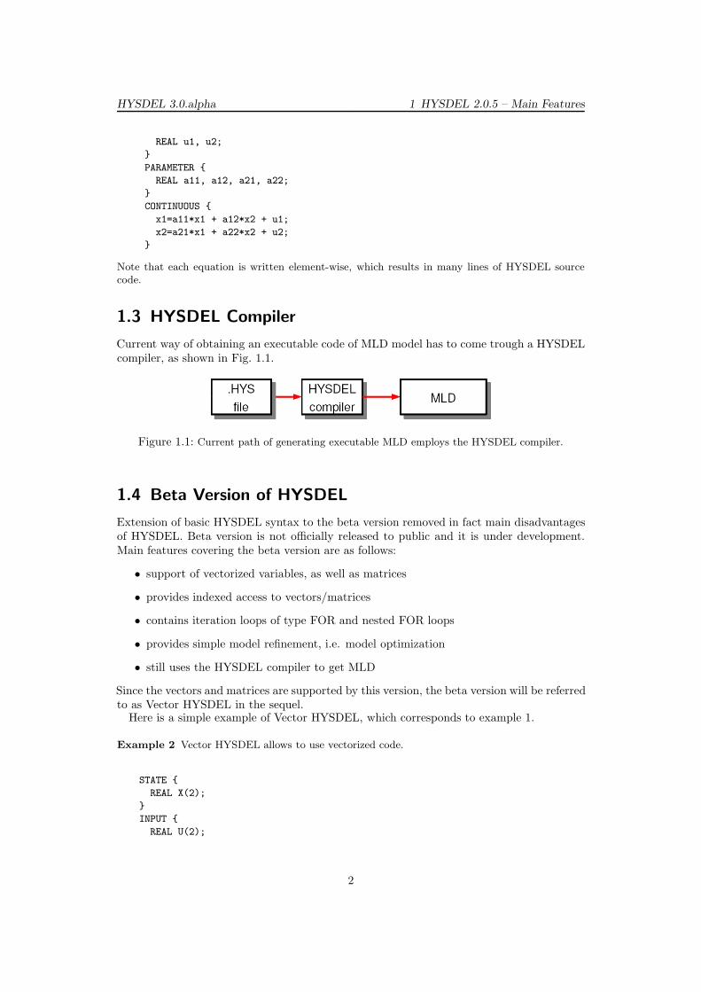
1.3 HYSDEL Compiler

Current way of obtaining an executable code of MLD model has to come trough a HYSDELcompiler, as shown in Fig. 1.1.

Figure 1.1: Current path of generating executable MLD employs the HYSDEL compiler.

1.4 Beta Version of HYSDEL

Extension of basic HYSDEL syntax to the beta version removed in fact main disadvantagesof HYSDEL. Beta version is not officially released to public and it is under development.Main features covering the beta version are as follows:

• support of vectorized variables, as well as matrices

• provides indexed access to vectors/matrices

• contains iteration loops of type FOR and nested FOR loops

• provides simple model refinement, i.e. model optimization

• still uses the HYSDEL compiler to get MLD

Since the vectors and matrices are supported by this version, the beta version will be referredto as Vector HYSDEL in the sequel.

Here is a simple example of Vector HYSDEL, which corresponds to example 1.

Example 2 Vector HYSDEL allows to use vectorized code.

STATE {

REAL X(2);

}

INPUT {

REAL U(2);

2

HYSDEL 3.0.alpha 1 HYSDEL 2.0.5 – Main Features

}

PARAMETER {

REAL A=[0.1,1; 0, 0.5];

}

CONTINUOUS {

X = A*X + U;

}

Although the size of HYSDEL code is reduced, the operation involved in processing such file stillremains complete, as will be shown in the sequel.

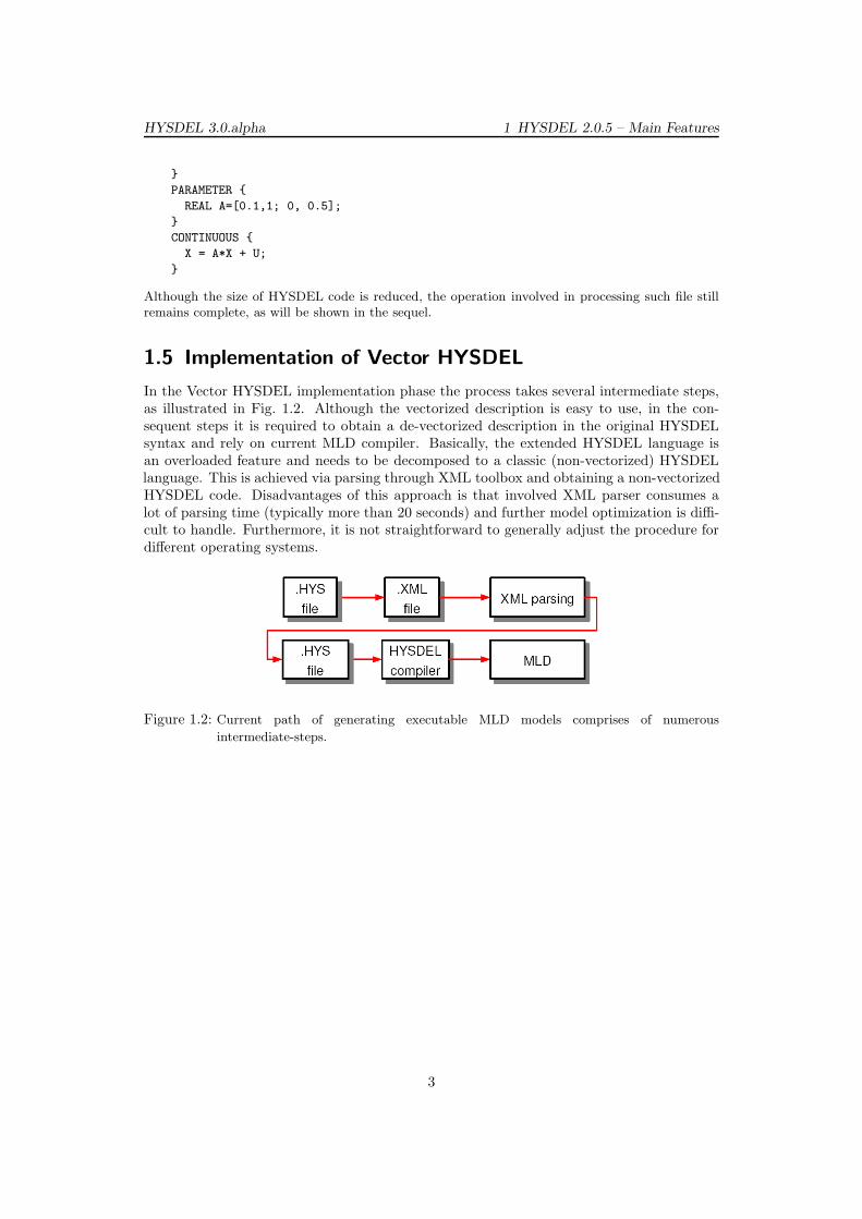
1.5 Implementation of Vector HYSDEL

In the Vector HYSDEL implementation phase the process takes several intermediate steps,as illustrated in Fig. 1.2. Although the vectorized description is easy to use, in the con-sequent steps it is required to obtain a de-vectorized description in the original HYSDELsyntax and rely on current MLD compiler. Basically, the extended HYSDEL language isan overloaded feature and needs to be decomposed to a classic (non-vectorized) HYSDELlanguage. This is achieved via parsing through XML toolbox and obtaining a non-vectorizedHYSDEL code. Disadvantages of this approach is that involved XML parser consumes alot of parsing time (typically more than 20 seconds) and further model optimization is diffi-cult to handle. Furthermore, it is not straightforward to generally adjust the procedure fordifferent operating systems.

Figure 1.2: Current path of generating executable MLD models comprises of numerous

intermediate-steps.

3

2 HYSDEL 3.0.alpha – Features

This chapter describes new features available in the version 3.0.alpha of the HYSDEL. Theaim will be to focus on differences comparing to HYSDEL 2.0.5 version and interpret thenew syntax on simple examples.

2.1 Extended Description of MLD system

To overcome identified shortcomings of the description (1.1) the model is rewritten into moreconvenient form. Arising from requirement, that each variables should be clearly distinct,new notations are adopted. More precisely, the new MLD description is given by

x(k + 1) = Ax(k) + Buu(k) + Bauxw(k) + Baff (2.1a)

y(k) = Cx(k) + Duu(k) + Dauxw(k) + Daff (2.1b)

Exx(k) + Euu(k) + Eauxw(k) ≤ Eaff (2.1c)

{indices} Jx, Ju, Jw, Jeq (2.1d)

where the auxiliary vector w(k) comprises of two elements w(k) = [δ(k), z(k)]T . Comparingto previous description (1.1), these changes are visible

• matrices B1, D1, and E1 are referred to as Bu, Du, and Eu, respectively

• auxiliary variables δ(k) and z(k) are merged together in one vector called w(k) =[δ(k), z(k)]T

• matrix couples B2 - B3, D2 - D3, E2 - E3 are referred to as Baux = [B2 B3], Daux =[D2 D3], Eaux = [E2 E3], respectively

• affine terms Baff , Daff are included

• E4 and E5 are now referred to as Ex and Eaff , respectively. Moreover, since inequal-ity (2.1c) is written in a standard form, i.e. Av ≤ b, and comparing to (1.1), theirrelations are Ex = −E4 and Eu = −E1.

• indices (2.1d) indicate which variables are real, and which are binary for states Jx,inputs Ju, auxiliary variables Jw and additionally, Jeq corresponds to indices withequality constraints

Structure of the indexed sets Jx, Ju, Jw is column-wise, distinguishing between binaryand real variables with strings. Precisely, string ’r’ refers to real and string ’b’ refers tobinary/Boolean variable, e.g.

{Jx, Ju, Jw} =

’r’

’r’

’b’

’r’

corresponds to

REAL

REAL

BOOL

REAL

4

HYSDEL 3.0.alpha 2 HYSDEL 3.0.alpha – Features

To determine location of equality constraints, the vector of indices Jeq will refer to theircorresponding rows in (2.1c), e.g.

Jeq =

158

corresponds to

1st row is an equality constraint5th row is an equality constraint8th row is an equality constraint

[Although labeling by strings clearly helps to distinguish the type of variables, it is notsuitable for further operations based on indexing. For this purpose, the information aboutthe position of variables in a vector will be stored in a substructure ’j’. Notation remainsthe same as in 2.0.5 version, and internal access is Matlab-like, e.g.]

S.j.xr /* indices of REAL states */

.j.xb /* indices of BOOL states */

.j.ur /* indices of REAL inputs */

.j.ub /* indices of BOOL inputs */

.j.yr /* indices of REAL outputs */

.j.yb /* indices of BOOL outputs */

.j.d /* indices of BOOL auxiliary variables */

.j.z /* indices of REAL auxiliary variables /*

.j.eq /* indices of equality constraints */

.j.ineq /* indices of inequality constraints */

Remaining notations of HYSDEL 2.0.5 remain the same, e.g. dimension of the statenx, or binary state nxr, etc. Once the HYSDEL file proceeds through the compiler wholeinformation will be stored in a structure format called S. Access to internal variables isMatlab-like, for instance one can access the dimension of states is as S.nx, and dimensionof states of type real as S.nxr. Matrices introduced in MLD model (2.1) will be stored as

S.A

.Bu

.Baux

.Baff

.C

.Du

.Daux

.Daff

.Ex

.Eu

.Eaux

.Eaff

Dimensions of the variables will have the following notations

S.nx /* dimension of states */

.nu /* dimension of inputs */

.ny /* dimension of outputs */

.nw /* dimension of auxiliary variables */

.nc /* dimension of constraints (equalities + inequalities) */

and indexed set will be accessible through

5


S.J.X /* string of indices (’r’ or ’b’) for states */

.J.U /* string of indices (’r’ or ’b’) for inputs */

.J.Y /* string of indices (’r’ or ’b’) for outputs */

.J.W /* string of indices (’r’ or ’b’) for auxiliary variables */

.J.eq /* numerical indices of equality constraints */

2.2 HYSDEL Language

This section points out the main differences comparing to old HYSDEL language. Thestructure follows the syntactical parts of HYSDEL scripting language. Before proceedingfurther, basics of the HYSDEL language will be given.

2.2.1 Preliminaries

A HYSDEL syntax was developed on C-language, and many symbols are similar. Struc-turally, a standard HYSDEL file comprises of two modes, namely INTERFACE and IM-PLEMENTATION. Each of the sections is delimited by curly brackets e.g.

section {

...

}

and this holds for every kind of subsections as well. If one wants to add comments, this issimply done via C-like comments, i.e.

section {

...

/* this line is commented */

...

}

An example of the simplest HYSDEL file might look as follows

SYSTEM name {

/* example of HYSDEL file structure */

INTERFACE {

/* interface part serves as declaration of variables */

}

IMPLEMENTATION {

/* implementation part defines relations between declared variables */

}

}

Note that the file begins with SYSTEM string which is followed by the name. The namecan be arbitrary, but it should be kept in mind that it usually points to a real object,therefore is recommended to use labels as e.g. tank, valve, pump, belt, etc. Other stringslike INTERFACE and IMPLEMENTATION are obligatory. HYSDEL file can be createdwithin any preferred text editor, however, the file should always have the suffix “.hys”, e.g.tank.hys. More importantly, it is recommended to use the name of the SYSTEM also asthe file name, e.g. system called tank will be a file tank.hys etc. This becomes reasonableif there are more HYSDEL files in one directory and helps to identify the files easily. In thenext content, the aim is to interpret new syntactical changes comparing to HYSDEL 2.0.5version.

6


2.2.2 List of Language Changes

The list of topics of syntactical changes in HYSDEL 3.0.alpha is briefly summarized in thesequel, while the details will be explained in particular sections.

• INTERFACE section

– extensions of the INTERFACE section

– declaration of INPUT, STATE, OUTPUT variables in scalar/vectorized form

– declaration of parameters

– declaration of subsystems

• IMPLEMENTATION section

– extensions of the IMPLEMENTATION section

– indexing

– FOR and nested FOR loops

– access to symbolic parameters

– operators and built-in functions

– AUX section

– CONTINUOUS section

– AUTOMATA section

– LINEAR section

– LOGIC section

– AD section

– DA section

– MUST section

– OUTPUT section

• Merging of HYSDEL files

2.2.3 INTERFACE Section

The INTERFACE section defines the main variables which appear for the given SYSTEM.More precisely, this section defines input, state and output variables distinguished by stringsINPUT, STATE and OUTPUT. Moreover, additional variables which do not belong to theseclasses are supposed to be declared in the section called PARAMETER. A new feature ofthis version is that sometimes the block SYSTEM may contain other subsystems and thisblock should describe the overall behavior of the system. If this is the case, the MODULEsection is to be present where subsystems are declared. This is the main change contrary toprevious version.

Syntactical structure of the INTERFACE section has the following structure

INTERFACE { interface_item }

which comprises of curly brackets and interface item. The interface item may take onlyfollowing forms

/* allowed INTERFACE items */

MODULE { /* module_item */ }

INPUT { /* input_item */ }

7


STATE { /* state_item */ }

OUTPUT { /* output_item */ }

PARAMETER { /* parameter_item */ }

where each item appears only once in this section. Each interface item is separated at leastwith one space character and may be omitted, if it is not required. The order of each itemcan be arbitrary, it does not play a role for further processing.

Example 3 A structure of a standard HYSDEL file is shown here, where the INTERFACE itemsare separated by paragraphs, and curly brackets denote visible start- and end-points of each section.

SYSTEM name {

/* example of HYSDEL file */

INTERFACE {

/* declaration of variables, subsystems */

MODULE {

/* declaration subsystems */

...

}

INPUT {

/* declaration input variables */

...

}

STATE {

/* declaration state variables */

...

}

OUTPUT {

/* declaration output variables */

...

}

PARAMETER {

/* declaration of parameters */

...

}

}

IMPLEMENTATION {

/* relations between declared variables */

...

}

}

Related subsections of the INTERFACE part will be explained in more detailed in the sequel.

INPUT section

In the input section are declared input variables of the SYSTEM which can be of type REAL(i.e. ur ∈ R), and BOOL (i.e. ub ∈ {0, 1}). General syntax of the INPUT section remainsthe same, i.e.

INPUT { input_item }

where each new input item is separated by at least one character space but the syntax ofinput item differs for real and binary variables. The input item for real variables takes theform of

8


REAL var [var_min, var_max];

where the string REAL, which denotes the type, is followed by var referring to name of theinput variable, the strings [var min, var max] express the lower and upper bounds, andsemicolon “;” denotes the end of the input item. If there are more than one input variables,they are separated by commas “,”, i.e.

REAL var1 [var_1_min, var_2_max], var2 [var_2min, var_2_max];

Example 4 Declaration of the scalar variable called “input flow”, which is bounded between 0 and10 m3/s will take the form

REAL input_flow [0, 10];

The input item for Boolean variables takes the form of

BOOL var;

where the string BOOL, which denotes the type, is followed by var referring to name of theinput variable, and semicolon “;” denotes the end of the input item. Here the specificationof bounds is not necessary because they are known but if even despite this one specifies thebounds on Boolean variables, HYSDEL will report an error. For more than one variables,separation by commas “,” is required, i.e.

BOOL var1, var2, var3;

Example 5 Declaration of the scalar Boolean variables called “switch” and “running” will takethe form

BOOL switch, running;

The main change comparing to previous version is that input variables may be definedas vectors, whereas the dimension of the input vector of real variables is nur and nub forbinary variables. This allows to define vectorized variables in the meaning of ur ∈ R

nur ,ub ∈ {0, 1}nub and the corresponding syntax is as follows

REAL var(nur) [var_1_min, var_1_max;

var_2_min, var_2_max;

..., ...;

var_nur_min, var nur_max];

for variables of type REAL and

BOOL var(nub);

for Boolean variables. Note that according to expression in normal brackets “(“ “)”, whichdenotes the dimension of the vector, the lower and upper bounds are specified for each vari-able in this vector. These bounds are separated by commas “,” and semicolon “;” denotes theend of row. If one declares variable in this way HYSDEL inherently assumes a column vector.

Note that the dimension of vector has to be always scalar and integer valued from the setN+ = {1, 2, . . .} and a particular value has to be always assigned. If the dimension of thevector is a symbolical parameter, HYSDEL will report an error. This holds similarly forSTATE, OUTPUT and PARAMETER section.

9


Example 6 We want to declare the input real vector ur ∈ R3 where the first variable may vary

in ur1 ∈ [−1, 2], the second variable in ur2 ∈ [0.5, 1.3], and the third variable in ur3 ∈ [−0.5, 0.5].Moreover, Boolean inputs of length 2, i.e. ub ∈ {0, 1}2 are present. The declaration of the INPUTsection will take the form

INPUT {

REAL ur(3) [-1, 2; 0.5, 1.3; -0.5, 0.5];

BOOL ub(2);

}

where it is not required to separate the lower and upper bounds into rows of the HYSDEL code.Important is that the semicolon as separator is present.

STATE section

STATE section declares state variables of the SYSTEM which can be of type REAL (i.e.xr ∈ R), and BOOL (i.e. xb ∈ {0, 1}) similarly as in the INPUT section. In general, thesyntax of the STATE section is as follows

STATE { state_item }

where each new state item is separated by at least one character space but the particularsyntax of state item differs for real and binary variables. The state item for real variablestakes the form of


where the string REAL, which denotes the type, is followed by var referring to name of theinput variable, the strings [var min, var max] express the lower and upper bounds, andsemicolon “;” denotes the end of the state item. If there are more than one input variables,they are separated by commas “,”, i.e.

REAL var1 [var_1_min, var_2_max], var2 [var_2_min, var_2_max];

Example 7 Declaration of the scalar variables called “position”, which is bounded between 0 and100 m, and “speed” (bounded from -10 to 10), will take the form

REAL position [0, 1000], speed [-10, 10];

The state item for Boolean variables takes the form of

BOOL var;

where the string BOOL, which denotes the type, is followed by var referring to name of theBoolean state, and semicolon “;” denotes the end of the state item. For more than onevariables, separation by commas “,” is required, i.e.

BOOL var1, var2, var3;

Example 8 Declaration of the scalar Boolean state called “is open” will take the form

BOOL is_open;

The main syntax difference, comparing to previous version, is that both REAL and BOOLvariables may be defined as vectors. Denoting the dimension of the real state vector asnxr and dimension of Boolean state vector nxb allows one to define vectors in the sense ofxr ∈ R

nxr , xb ∈ {0, 1}nxb and the corresponding syntax is as follows

10


REAL var(nxr) [var_1_min, var_1_max;

var_2_min, var_2_max;

..., ...;

var_nxr_min, var nxr_max];

for variables of type REAL and

BOOL var(nxb);

for Boolean variables. Note that according to expression in normal brackets “(“ “)”, whichdenotes the dimension of the vector, the lower and upper bounds are specified for eachvariable in this vector. These bounds are separated by semicolon “;” for each row. If onedeclares variable in this way HYSDEL inherently assumes a column vector.

Example 9 We want to declare the state real vector xr ∈ R2 where the first variable may vary in

xr1 ∈ [−1, 1], and the second variable in xr2 ∈ [0, 1]. Moreover, one Boolean state is present. Thedeclaration of the STATE section will take the form

STATE {

REAL xr(2) [-1, 1; 0, 1];

BOOL xb;

}

which defines a real vector xr in dimension 2 and scalar Boolean state xb.

Note that without specifying dimension of the variable, it is always considered as scalarvalue.

OUTPUT section

In the OUTPUT section, output variables of the SYSTEM are to be declared. These variablescan be of type REAL (i.e. yr ∈ R), and BOOL (i.e. yb ∈ {0, 1}), similarly as in the INPUTand STATE section. In general, the syntax of the OUTPUT section is as follows

OUTPUT { output_item }

where each new output item is separated by at least one character space and differs for realand binary variables. The output item for real variables takes the form of

REAL var;

where the string REAL, which denotes the type, is followed by var referring to name of theinput variable. More variables are delimited by commas “,” as in the INPUT and STATEsection.

Note that in the OUTPUT section no bounds are specified. It is because the output vari-able is always considered as an affine function of states and inputs, thus their bounds areautomatically inferred.

Example 10 Declaration of the scalar output variables called “y1” and “y2” will be as follows

REAL y1, y2;

where no bounds are specified.

11


The output item for Boolean variables takes the form of

BOOL var;

where the string BOOL, which denotes the type, is followed by var referring to name of theBoolean state, and semicolon “;” denotes the end of the state item. If there are more outputvariables, they are delimited by commas “,”.

Example 11 Declaration of the scalar Boolean output variables “d1”, “d2”, and “d3” will takethe form

BOOL d1, d2, d3;

which is the same as in HYSDEL 2.0.5.

Comparing to previous version, output variables may be defined as vectors. Denoting thedimension of the real output vector as nyr and dimension of Boolean output vector nyb

allows one to define vectors in the sense of yr ∈ Rnyr , yb ∈ {0, 1}nyb and the corresponding

syntax is then straightforward

REAL var(nyr);

for variables of type REAL where nyr denotes the dimension and

BOOL var(nub);

for Boolean variables with nub specifying the dimension of the column vector.

Example 12 We want to declare the output real vector yr ∈ R2, the second output real vector

q ∈ R2 and one binary vector outputs d ∈ {0, 1}3

OUTPUT {

REAL yr(2), q(2);

BOOL d(3);

}

Note that declaring the binary output in vectorized form is similar to example 11, but in this caseis shorter.

PARAMETER section

The PARAMETER section declares variables which will be treated as constants throughwhole HYSDEL file structure. In this case the syntax of the PARAMETER section is asfollows

PARAMETER { parameter_item }

where each parameter item may take one of the following forms

• declaration of constants

type var = value;

• declaration of constant column vectors with dimension n (the dimension does not haveto be present for constants)

type var = [value_1; value_2; ..., value_n];

12


• declaration of constant matrices with dimensions n×m (the dimension does not haveto be present for constants)

type var = [value_11, value_12, ..., value_1m;

value_21, value_22, ..., value_2m;

..., ..., ..., ...;

value_n1, value_n2, ..., value_nm];

where type can be either REAL or BOOL. If there are more parameters with constantvalues, they have to be separated using semicolons “;” as new variable, i.e.

type var1 = value1; type var2 = value2;

type var3 = value3;

Notations in vector and matrix description remain the same as in INPUT, STATE andOUTPUT section. That is, each element of the row is delimited with comma “,” and therow ends with semicolon “;” .

Example 13 We want to declare constants a = 1 as Boolean variable, b = [−1, 0.5, −7.3]T and

D =

„

−1 0 0.230.12 −0.78 2.1

«

as real variables. This can be done as follows

PARAMETER {

BOOL a = 1; REAL b = [-1; 0.5; -7.3];

REAL D = [-1, 0, 0.23; 0.12, -0.78, 2.1];

}

Moreover, PARAMETER section also allows symbolic parameters of type REAL, assumingthat their values will be specified later. If the parameter is symbolic, its declaration reads

PARAMETER {

type var; /* symbolic scalar */

type var(n); /* symbolic vector */

type var(n,m); /* symbolic matrix */

}

where the string type is either REAL or BOOL and the variable var can be scalar, vectorwith n rows, or matrix with dimensions n and m.

Note that dimension of symbolic vectors/matrices, i.e. n, m must not be symbolic parame-ters.

However, the presence of symbolic variables leads to bad conditioning of the resulting MLDmodel and therefore it is always required to assign particular values to symbolical expressionsbefore compilation.

If there is a strong need to keep symbolic parameter is MLD models, it is recommendedto specify lower and upper bounds on each declared symbolic parameter. The syntax in thiscase is similar to INPUT, STATE and OUTPUT section,


whereas the declared variable var can be only scalar. If there are more symbolic values,they are separated by commas “,”.

13


Note that huge number of symbolic parameters may prolong the compilation time as thenumber of involved operations is sensitive on symbolic expressions. Furthermore, symbolicexpressions have to be replaced with exact values, if the HYSDEL model is going to befurther processed.

HYSDEL language supports several numerical expressions, here is example of allowed for-mats

REAL a = 1.101;

REAL tol = 1e-3;

REAL eps = 0.5E-4;

REAL Na = 6.0221415e+23;

where the decimal number is separated with dot “.” and the decadic power is correspondsto sign “e” or “E”, i.e. 2.03×10−2 is written as 2.03e-10. Additionally, HYSDEL languagehas a set of predeclared variables, to which it suffices to refer with a given string. Precisely,

pi; /* pi = 3.141592653 */

MLD_epsilon; /* 1e-6 */

and their values can be overridden by the user.

Example 14 We want to declare boolean constant vector h = [1, 0, 1]T , real matrix A =„

π −0.05 × 102

−0.8 12 × 10−3

«

, symbolic vector v ∈ R2, and symbolic value p which may vary between

[−0.5, 1.8]. The HYSDEL syntax will take the form

PARAMETER {

BOOL h = [1; 0; 1]; /* constant vector */

REAL A = [pi, -0.05e2; -0.8, 12E-3]; /* constant matrix */

REAL v(2); /* symbolic vector, will be replaced with real

value before compilation */

REAL p [-0.5, 1.8]; /* symbolic parameter, which remains

symbolic also after compilation * /

}

MODULE section

The MODULE section is a new feature of HYSDEL 3.0.alpha which allows to create sub-systems. This is important especially when creating larger HYSDEL structures. To be ableto recognize which subsystem is a part of which system a concept of master and slave filesis adopted. A slave file will be referred to as a system, which is a part of bigger system, hasits own inputs, outputs and acts independently. A master file consist of at least one slavefile while inputs and outputs are created by subsystems.

Example 15 Example of a standard HYSDEL slave file, without any subsystems (i.e. without theMODULE section)

SYSTEM valveA {

/* example of slave HYSDEL file referring to a valveA */

INTERFACE {

/* declaration of variables */

INPUT { ... }

STATE { ... }

14


OUTPUT { ... }

PARAMETER { ... }

}

IMPLEMENTATION {


}

}

The syntax of the MODULE section is given by

MODULE { module_item }

where each of the module item is composed of

name par;

The string name refers to a name of the subsystem which contains parameter par. If thereare more parameters, they are separated by commas, i.e.

name par1, par2, par3;

The syntax is similar to defining symbolical parameters in the PARAMETER section whilethe exact values have to be assigned in the PARAMETER section before compilation.

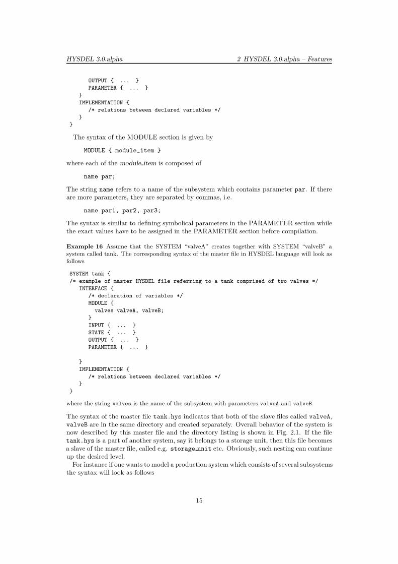
Example 16 Assume that the SYSTEM “valveA” creates together with SYSTEM “valveB” asystem called tank. The corresponding syntax of the master file in HYSDEL language will look asfollows

SYSTEM tank {

/* example of master HYSDEL file referring to a tank comprised of two valves */

INTERFACE {

/* declaration of variables */

MODULE {

valves valveA, valveB;

}

INPUT { ... }

STATE { ... }

OUTPUT { ... }

PARAMETER { ... }

}

IMPLEMENTATION {


}

}

where the string valves is the name of the subsystem with parameters valveA and valveB.

The syntax of the master file tank.hys indicates that both of the slave files called valveA,valveB are in the same directory and created separately. Overall behavior of the system isnow described by this master file and the directory listing is shown in Fig. 2.1. If the filetank.hys is a part of another system, say it belongs to a storage unit, then this file becomesa slave of the master file, called e.g. storage unit etc. Obviously, such nesting can continueup the desired level.

For instance if one wants to model a production system which consists of several subsystemsthe syntax will look as follows

15


Figure 2.1: Example of a SYSTEM tank containing two subsystems valveA, valveB and corre-

sponding directory listing.

SYSTEM production {

INTERFACE {

MODULE {

storage_tank tank1, tank2;

conveyor_belt belt;

packaging packer;

}

/* other section are omitted */

}

where the slave files are determined via name of the subsystem and corresponding files.

2.2.4 IMPLEMENTATION Section

Relations between variables are determined in the IMPLEMENTATION section. Accordingto type of variables, this section is further partitioned into subsections, which remain thesame as in previous version. Syntactical structure of the IMPLEMENTATION section hasthe following form

IMPLEMENTATION { implementation_item }

which comprises of curly brackets and implementation item. The implementation item maytake only following forms

AUX { /* aux_item */ }

CONTINUOUS { /* continuous_item */ }

AUTOMATA { /* automata_item */ }

LINEAR { /* linear_item }

LOGIC { /* logic_item }

AD { /* ad_item */ }

DA { /* da_item */ }

MUST { /* must_item */ }

OUTPUT { /* output_item */ }

where each item appears only once in this section. Each implementation item is separatedat least with one space character and may be omitted, if it is not required. The order ofeach item can be arbitrary, it does not play a role for further processing.

Note that OUTPUT section is also present as in the INTERFACE part but here it hasdifferent syntax and semantics.

16


New changes in the IMPLEMETATION section affect the syntax of each subsection andthe common features are listed as follows:

• indexing

• FOR and nested FOR loops

• operators and built-in functions

These changes will be explained first, before describing the individual changes in each IN-TERFACE subsection.

Example 17 A structure of the standard HYSDEL file is given next where the meaning of eachsubsection of the IMPLEMENTATION part is briefly explained

SYSTEM name {

INTERFACE {

/* declaration of variables, subsystems */

}

IMPLEMENTATION {


AUX {

/* declaration of auxiliary variables, needed for

calculations in the IMPLEMENTATION section */

}

CONTINUOUS {

/* state update equation for variables of type REAL */

}

AUTOMATA {

/* state update equation for variables of type BOOL */

}

LINEAR {

/* linear relations between variables of type REAL */

}

LOGIC {

/* logical relations between variables of type BOOL */

}

AD {

/* analog-digital block, specifying relations between

variables of type REAL to BOOL */

}

DA {

/* digital-analog block, specifying relations between

variables of type BOOL to REAL */

}

MUST {

/* specification of input/state/output constraints */

}

OUTPUT {

/* selection of output variables which can be of type

REAL or BOOL) */

}

}

}

17


Indexing

Introducing vectors and matrices induced the extension of the HYSDEL language to useindexed access to internal variables. The syntax is different for vectors and matrices since itdepends on the dimension of the variable. Access to vectorized variables has the followingsyntax

new_var = var(ind);

where new var denotes the name of the auxiliary variable (must be defined in AUX section),var is the name of the internal variable and ind is a vector of indices, referring to positionof given elements from a vector. Indexing is based on a Matlab syntax, where the argumentind must contain only N+ = {1, 2, . . .} valued elements and its dimension is less or equalto dimension of the variable var. Syntax of the ind vector can be one of the following:

• increasing/decreasing sequence

ind_start:increment:ind_end

where ind start denotes the starting position of indexed element, increment is thevalue of which the starting value increases/decreases, and ind end indicates the endposition of indexed element.

• increasing by one sequence

ind_start:ind_end

where the value increment is now omitted and HYSDEL automatically treats thevalue as +1

• particular positions

[pos_1, pos_2, ..., pos_n]

where pos 1, ..., pos n indicates the particular position of elements

• nested indices

ind(sub_ind)

where the vector ind is sub-indexed via the aforementioned ways by vector sub ind

with N+ values

Example 18 In the parameter section were defined two variables. The first variable is a constantvector h = [−0.5, 3, 1, π, 0]T and the second variable is a symbolical expression g ∈ R

3, g1 ∈[−1, 1], g2 ∈ [−2, 2], g3 ∈ [−3, 3]. We want to assign new variables z and v for particular elementsof these vectors. Examples are:

• increasing sequence, e.g. z = [−0.5, 1, 0]T

z = h(1:2:5);

• decreasing sequence, e.g. v = [g3, g2]T

v = g(3:-1:2);

18


• increasing by one, e.g. z = [1, π, 0]T

z = h(3:5);

• particular positions, e.g. v = [g1, g3]T

v = g([1,3]);

• nested indexing, e.g. z = [3, π]T , k = [2, 3, 4]

z = h(k([1, 3]));

where the variable k has to be declared first.

Indexing of matrices is similar, however, in this case two indices are required. The indexedsyntax takes the following form

new_var = var(ind_row,ind_col);

where new var denotes the name of the auxiliary variable (must be defined in AUX section),var is the name of the internal variable, ind row is a vector of indices referring to rows, andind col is a vector of indices referring to columns.

Note that indexing is based on a Matlab syntax, where the argument ind must contain onlyN+ = {1, 2, . . .} valued elements and its dimension is less or equal to dimension of thevariable var.

Syntax of the items ind row, ind col is the same as for vectors the item ind.

Example 19 In the parameter section a constant matrix is defined

A =

0

@

0 −5 −0.8 1−2 0.3 0.6 −1.20.5 0.1 −3.2 −1

1

A

We may extract values from matrix A to form new variable B as follows

• increasing sequence, e.g.

B =

„

0 −5−2 0.3

«

B = A(1:2,1:2);

• decreasing sequence, e.g.

B =

0

@

0.5 0.1 −3.2 −1−2 0.3 0.6 −1.20 −5 −0.8 1

1

A

B = A(3:-1:1,1:4);

• particular positions, e.g. B = [0, 0.3, −3.2]T

B = A(1:3,[1, 2, 3]);

• nested indexing, e.g. B = [0.6, −1.2]T , irow = [2, 3], icol = [1, 2, 3, 4]

B = h(i_row,i_col(3:4));

where the variables i row and i col have to be declared first.

19


FOR loops

FOR loops are another important feature of HYSDEL 3.0.alpha version. To create a repeatedexpression, one has to first define an iteration counter in the AUX section according to syntax

AUX {

INDEX iter;

}

where the prefix INDEX denotes the class, and iter is the name of the iteration variable. Ifthere are more iteration variables required, the additional variables are separated by commas“,”, i.e.

AUX {

INDEX iter1, iter2, iter3;

}

As the iteration variable is declared, the FOR syntax takes the form of

FOR ( iter = ind ) { repeated_expr }

where the string FOR is followed by expression in normal brackets “(”, “)” and expressionin curly brackets “{”, “}”. The expression in normal brackets is characterized by assign-ment iter = ind where the iteration variable iter incrementally follows the set defined byvariable ind and this variable takes one of the form shown in section indexing 2.2.4. Theexpression in curly brackets named repeated expr is recursively evaluated for each value ofiterator iter and can take the form of

aux_item

continuous_item

automata_item

linear_item

logic_item

ad_item

da_item

must_item

output_item

depending in which section the FOR loop lies. This allows to use the FOR loop within thewhole IMPLEMENTATION section.

Example 20 Suppose, that it is required to repeat ad item in the AD section for each binaryvariable di if state xri ≥ 0, i = 1, 2, 3, i.e.

d1 = xr1 ≥ 0

d2 = xr2 ≥ 0

d3 = xr3 ≥ 0

The iteration index, as well as auxiliary Boolean variable d has to defined first,

AUX {

INDEX i;

BOOL d(3);

}

20


and they can be consequently used in the AD section as follows

AD {

FOR (i=1:3) { d(i) = xr(i) >= 0; }

}

HYSDEL 3.0.alpha supports also nested loops. In this case the syntax remains the same,but the repeated expr have now the structure of

FOR ( iter = ind ) { repeated_expr }

which does not differ from the syntax outlined above.

Example 21 Suppose that we want to code a matrix multiplication for state update equation ofthe form

„

xr1(k + 1)xr2(k + 1)

«

=

„

1 0.50.2 0.9

« „

xr1(k)xr2(k)

«

+

„

10

«

ur(k)

Assuming that vectors x, u are already declared, we also declare constant matrices in the INTER-FACE section

PARAMETER {

REAL A = [1, 0.5; 0.2, 0.9];

REAL B = [1; 0];

}

Secondly, we define iteration counters in IMPLEMENTATION section

AUX {

INDEX i,j;

}

and then use the nested loop syntax as follows

CONTINUOUS {

FOR (i=1:2) {

x(i) = 0;

FOR (j=1:2) { x(i) = A(i,j)*x(j) + x(i); }

x(i) = x(i) + B(i)*u;

}

}

Example 22 FOR loops allow also to more complicated expressions. For instance, indexing in apower sequence 2i where i = 1, . . . , 5. Assume that for given vector h ∈ R

32 it is required to assigna real variable z ∈ R

5 according to power sequence indexing. In HYSDEL it can be written asfollows

FOR (i=1:5) { z(i) = h(2^i); }

where the variables i, z, and h were previously declared.

Accessing Symbolic Parameters

Symbolic parameters allow more flexibility when creating MLD models. They are declaredin the PARAMETER section and in the MODULE section independently, but access is thesame. In general, the access is like in Matlab structures. For a standard HYSDEL slave file(which does not have any MODULE section) the syntax takes the common form

21


SYSTEM name {

INTERFACE {

/* other parts are omitted */

...

PARAMETER {

type var;

type var(n);

type var(n,m);

type var [var_min, var_max];

}

}

IMPLEMENTATION {


}

}

and after compilation the symbolic variables are stored in a structure called S under fieldsparams, i.e.

S.params.var

If the HYSDEL file contains a MODULE section it is built from subsystems declared in thissection. The parameters of the subsystems can be now replaced with concrete values, usingthe following syntax

SYSTEM master {

INTERFACE {


MODULE {

subsystem name1, name2;

}

PARAMETER {

name1.var = value1;

name2.var = value2;

}

}

IMPLEMENTATION {


}

}

In the remaining IMPLEMENTATION section the symbolical values will be automaticallyreplaced with numerical values.

Example 23 Suppose that a master file tank is created by two subsystems valveA and valveB.Both of the slave file contains symbolical parameters height and width as in this example forvalveA

SYSTEM valveA {

INTERFACE {

/* some parts are omitted */

...

PARAMETER {

22


REAL width, height;

}

}

}

The exact values can be set in the master file as follows

SYSTEM tank {

INTERFACE {

/* some parts are omitted */

...

MODULE {

valves valveA, valveB;

}

PARAMETER {

valveA.width = 0.15;

valveA.height = 0.23;

valveB.width = 0.2;

valveB.height = 0.35;

}

}

}

HYSDEL operators and built-in functions

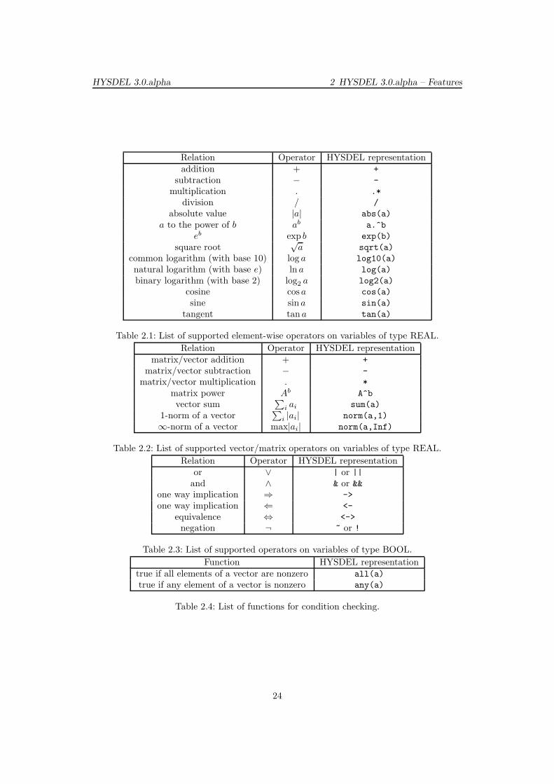
Throughout the whole HYSDEL file various relations between variables can be defined.Because the variables may be also vectors (matrices), the list of supported operators isdistinguished by

• element-wise operations, in Tab. 2.1

• and vector functions, in Tab. 2.2.

For Boolean variables HYSDEL supports operators, as summarized in Tab. 2.3. Additionally,syntactical functions are available, which allow condition checking and are summarized inTab. 2.4.

[toto neviem ci ma vobec zmysel udavat, lebo dovolene vyrazy uz mame definovane vaffine expr, etc. Ja by som to nasledovne uuplne vyhodil. ]

Since the variables may be constants as well as varying, the operators cannot be usedarbitrary. This holds especially for varying variables of type REAL (states, inputs, outputs,auxiliary). Denoting this group with notation v, only following relations are allowed

• relations between varying variables v1 and v2 of type REAL

– addition: v1 + v2

– subtraction: v1 - v2

• relations between varying variable v and constant parameter p of type REAL

– addition: v + p = p + v (v and p have the same dimension)

– subtraction: v − p = −p + v (v and p have the same dimension)

– multiplication: v ∗ p = p ∗ v (p is scalar)

– division: v/p = 1/p ∗ v (p is scalar except equal 0)

23


Relation Operator HYSDEL representationaddition + +

subtraction − -

multiplication . .*

division / /

absolute value |a| abs(a)

a to the power of b ab a.^b

eb exp b exp(b)

square root√

a sqrt(a)

common logarithm (with base 10) log a log10(a)

natural logarithm (with base e) ln a log(a)

binary logarithm (with base 2) log2 a log2(a)

cosine cos a cos(a)

sine sin a sin(a)

tangent tan a tan(a)

Table 2.1: List of supported element-wise operators on variables of type REAL.

Relation Operator HYSDEL representationmatrix/vector addition + +

matrix/vector subtraction − -

matrix/vector multiplication . *

matrix power Ab A^b

vector sum∑

i ai sum(a)

1-norm of a vector∑

i |ai| norm(a,1)

∞-norm of a vector max|ai| norm(a,Inf)

Table 2.2: List of supported vector/matrix operators on variables of type REAL.

Relation Operator HYSDEL representationor ∨ | or ||

and ∧ & or &&one way implication ⇒ ->

one way implication ⇐ <-

equivalence ⇔ <->

negation ¬ ~ or !

Table 2.3: List of supported operators on variables of type BOOL.

Function HYSDEL representationtrue if all elements of a vector are nonzero all(a)

true if any element of a vector is nonzero any(a)

Table 2.4: List of functions for condition checking.

24


• operations summarized in tables 2.1, 2.2, and 2.4 hold for relations between two pa-rameters p1, p2 of type REAL

• for variables of type BOOL are only Boolean expressions valid (Tab. 2.3. However,operations of type REAL can be used but only if the Boolean variable is retyped toclass REAL.

][Tu treba spomenut evaluaciu prednostnych operacii, ako aj zatvorkovanie - neviem, co

presne teraz hysdel podporuje. Na toto sa specialne pytali v ABB].[If in the expression two or more operators appear, their meaning will be evaluated se-

quentially, that is, no priorities are between operators. For instance, v = a + b ∗ c the resultis v = (a + b) ∗ c. ]

[If in the expression two or more operators appear, their evaluation is according to operatorpriority. That is for instance, v = a + b ∗ c will have the result is v = a + (b ∗ c).]

In general, it is recommended to use normal brackets “(“, “)” to separate variables intogroups and evaluate bracketed and hence prior expressions first. [Example?]

[Operators on symbolical expressions?]

AUX section

In the AUX section one has to declare auxiliary variables needed for derivations of furtherrelations in the IMPLEMENTATION section. The declaration of these variables followswith specifying the type of the variable (REAL, BOOL or INDEX) and defining the name,e.g.

type var;

where the string type can be REAL, BOOL or INDEX and it is followed by a variable var.If there are more variables, they are delimited by commas “,”.

Example 24 Suppose that in the AUX section we have to declare two iterators i, j, two realvectors z ∈ R

3, v ∈ R2 and Boolean variable d ∈ {0, 1}5. The AUX syntax takes the following form

AUX {

INDEX i,j; /* iteration counters */

REAL z(3),v(2); /* auxiliary REAL vectors */

BOOL d(5); /* auxiliary BOOL vector */

}

Contrary to INTERFACE section, here lower and upper bounds on the variables are notgiven. The values are automatically calculated from variables declared in the INTERFACEsection since AUX variables are affine functions of these variables. Moreover, no constants,as well as no parameters are here declared.

CONTINUOUS section

In the CONTINUOUS section the state update equations for variables of type REAL are tobe defined. The general syntax is given as

CONTINUOUS { continuous_item }

where the continuous item may be inside a FOR loop and takes the form

25


var = affine_expr;

The variable var corresponds to the state variable declared in the section STATE and itcan be scalar or vectorized expression. The affine expr is an affine function of parameters,inputs, states and auxiliary variables, which have been previously declared.

Note that only variables of type REAL, declared in STATE section can be assigned here.

Example 25 Suppose that the state update equation is driven by

x(k + 1) = Ax(k) + Bu(k) + f

where the matrices A, B, f are constant parameters, x is state, u is input. This can be written inHYSDEL language as short vectorized form, i.e.

CONTINUOUS {

x = A*x + B*u + f;

}

AUTOMATA section

The AUTOMATA section describes the state transition equations for variables of typeBOOL. The general syntax takes the form

AUTOMATA { automata_item }

where the automata item may be inside a FOR loop and is built by

var = Boolean_expr;

The variable var corresponds to the Boolean variable defined in the section STATE andit can be scalar or vectorized expression. The Boolean expr is a combination of Booleaninputs, Boolean states, and auxiliary Boolean variables with operators reported in Tab. 2.3.

Note that only variables of type BOOL, declared in STATE section can be assigned here.

Example 26 Suppose that the Boolean state update is driven by following relations

x2(k + 1) = u1(k) ∨ (u2(k) ∧ ¬x1(k))

Related HYSDEL syntax will take the form of

AUTOMATA {

xb(2) = ub(1) | (ub(2) & ~xb(1));

}

LINEAR section

In the LINEAR section it is allowed to define additional variables, which are build by affineexpressions of states, inputs, parameters and auxiliary variables of type REAL. In general,the structure of the LINEAR section is given by

LINEAR { linear_item }

where the linear item may be inside a FOR loop and takes the form of

26


var = affine_expr;

The variable var is of type REAL and was previously declared in the AUX section. Theaffine expr is an affine function of parameters, inputs, states and auxiliary variables of typeREAL, which have been previously declared.

Example 27 Consider that it is suitable to define an auxiliary continuous variable g = −0.5x1 +3which is an affine function of the state x ∈ R

2. The variable is firstly declared in the AUX section,

AUX {

REAL g;

}

and consequently, the expression in LINEAR section takes the form

LINEAR {

g = -0.5*x(1) + 3;

}

Furthermore, the LINEAR section is devoted to determine relations between subsystemsand applies only if there is MODULE section present. More precisely, the syntax is given by

var = linear_expr;

where the variable var access the internal input or output variable of type REAL of thedeclared subsystem. The linear expr is a linear function (i.e. without affine term) of internalinputs or output variables of type REAL of the declared subsystems. [Ma to byt skutocneiba linearna funkcia a nie affinna?] More detailed view for merging of subsystems will begiven in special section.

Note that LINEAR section serves also for declaration of interconnection between subsystems(if they are declared in MODULE section).

LOGIC section

LOGIC section allows to define additional relations between variables of type BOOL whichmight simplify the overall notations. In general the syntax is given by

LOGIC { logic_item }

where the logic item may be inside a FOR loop and is built by

var = Boolean_expr;

The variable var corresponds to the Boolean variable defined in the section AUX and it canbe scalar or vectorized expression. The Boolean expr is a combination of Boolean inputs,Boolean states, and auxiliary Boolean variables with operators reported in Tab. 2.3.

Example 28 Suppose that we want to introduce the Boolean variable d = x1 ∧ (¬x2 | ¬x3), whichis a function of Boolean states x ∈ {0, 1}3. We proceed first with variable declaration in AUXsection

AUX {

BOOL d;

}

and follow with LOGIC section

LOGIC {

d = x(1) & (~x(2) | ~x(3));

}

27


AD section

AD section is used to express the relations between variables of type REAL to Booleanvariables only with help of logical operator equivalence. Here, the equivalence operator <->

is replaced with = operator and the syntax is given as

AD { ad_item }

where the ad item might be inside a FOR loop and it can be one of the following

var = affine_expr >= real_num;

var = affine_expr <= real_num;

The variable var is of type BOOL and has to be declared in the AUX section. The affine expris a function of states, inputs, parameters and auxiliary variables of type REAL. Operator>= denotes the greater or equal inequality (≥) and operator <= is less or equal inequality(≤). Expression real num is a real valued number.

Example 29 Suppose that we want to assign to a Boolean variable d ∈ {0, 1}3 value 1 if certaininequality is satisfied, otherwise it will be 0.

d1 =

(

1 if x1 + 2u2 ≥ 0

0 otherwise, d2 =

(

1 if 0.5x2 − 3x3 ≤ 0

0 otherwise, d3 =

(

1 if x1 ≥ 1.2

0 otherwise

HYSDEL allows to model this behavior using AD syntax

AUX {

BOOL d(3);

}

AD {

d(1) = x(1) + 2*u(2) >= 0;

d(2) = 0.5*x(2) - 3*x(3) <= 0;

d(3) = x(1) >= 1.2;

}

Previous version required bounds on auxiliary variables var in the form of

var = affine_expr >= real_num [min, max, eps];

var = affine_expr <= real_num [min, max, eps];

but this syntax is obsolete and related bounds calculation are now obtained automatically.If the bounds will be provided anyway, HYSDEL will raise a warning.

Note that AD section does not use curly brackets “{“, “}” to assign the auxiliary variable.

DA section

The DA section defines continuous variables according to if-then-else conditions. HYSDEL3.0.alpha language supports the following syntax

DA { da_item }

where the da item might be inside a FOR loop or and it can be one of the following

var = { IF cond THEN affine_expr };

var = { IF cond THEN affine_expr ELSE affine_expr};

28


The variable var corresponds to auxiliary variable of type REAL, defined in the AUX section.Expression cond can be defined as

affine_expr >= real_num;

affine_expr <= real_num;

Boolean expr;

which denotes certain condition satisfaction. The affine expr is a function of states, inputs,parameters and auxiliary variables of type REAL. Operator >= denotes the greater or equalinequality (≥) and operator <= is less or equal inequality (≤). Expression real num is a realvalued number. The Boolean expr is a function of Boolean states, inputs, parameters andauxiliary variables combined with operators listed in Tab. 2.3.w

Note that if the ELSE string is missing, HYSDEL automatically treats the value equal 0.

Example 30 Suppose that we want to introduce an auxiliary variable z which depends on a con-tinuous state x and a binary input ub as follows

z =

(

x if ub = 1

−x if ub = 0

HYSDEL models this relation by

AUX {

REAL z;

}

DA {

z = { IF ub THEN x ELSE -x };

}

Example 31 It is also possible to define switching conditions using real expressions. Suppose thatwe want to introduce an auxiliary variable z which depends on continuous states x1 and x2

z =

(

2x1 if x2 ≥ 0

−x1 + 0.5x2 if x2 ≤ 0

HYSDEL 3.0.alpha allows to models this relation by

AUX {

REAL z;

}

DA {

z = { IF x(2) >= 0 THEN 2*x(1) ELSE -x(1)+0.5*x(2) };

}

and this syntax is more familiar to describe the behavior of PWA systems.

Similarly as in the AD section, previous version required bounds on variables

var = { IF cond THEN affine_expr [min, max, eps] };

var = { IF cond THEN affine_expr [min, max, eps]

ELSE affine_expr [min, max, eps] };

This syntax is obsolete and related bounds calculation is now performed automatically.HYSDEL will report a warning if this syntax will be used.

29


MUST section

MUST section specifies constraints on input, state, and output variables. Regardless of thetype of variables, it is required that these condition will be fulfilled for the whole time. TheMUST section takes the following syntax

MUST { must_item }

where the must item can be one of the following

real_cond;

Boolean_expr;

real_cond BO Boolean_expr;

Boolean_expr BO real_cond;

which denotes certain condition satisfaction. Expression real cond is given by

affine_expr >= real_num;

affine_expr <= real_num;

and BO is a Boolean operator from Tab. 2.3. The affine expr is a function of states, inputs,parameters and auxiliary variables of type REAL. Operator >= denotes the greater or equalinequality (≥) and operator <= is less or equal inequality (≤). Expression real num is a realvalued number. The Boolean expr is a function of Boolean states, inputs, parameters andauxiliary variables combined with operators listed in Tab. 2.3.

Example 32 Consider a system where the one input real variable ur ∈ R and five states xr ∈ R5.

Moreover, although the bounds on these variables have been declared, additional constraints areintroduced, which are subsets of the declared bounds, i.e. ur ∈ [−2, 2] and xr1 ∈ [−1, 5], xr2 ∈[−2, 3.4], xr3 ∈ [0.5, 2.8]. These constraints are written in MUST section as follows

MUST {

ur >= -2;

ur <= 2;

xr(1:3) >= [-1; -2; 0.5];

xr(1:3) <= [5; 3.4; 2.8];

}

Example 33 For binary variables, one way implications are allowed, as well as equivalence. Ex-ample is a system with binary inputs ub ∈ {0, 1}2 which implies that a value of auxiliary binaryvariable will we 0 or 1, e.g.

d1 ⇒ ub1, d2 ⇐ ub2, d3 ⇔ xb2

and it can be written in HYSDEL as

MUST {

d(1) -> ub(1);

d(2) <- ub(2);

d(3) <-> xb(2);

}

Example 34 HYSDEL 3.0.alpha supports also combined REAL–BOOL expressions. Consider astate vector x ∈ R

2, and binary input ub ∈ {0, 1}2. One may require the constraints as

ub1 ⇒ x1 ≥ 0,

x1 + 2x2 ≥ −2 ⇐ ¬ub2,

ub1 ∨ ub2 ⇔ x1 − x2 ≥ 1

and it can be written in HYSDEL as

30


MUST {

ub(10) -> x(1) >= 0;

x(1) + 2*x(2) <- ~ub(2);

ub(1) | ub(2) <-> x(1) - x(2) >= 1;

}

OUTPUT section

The OUTPUT section specifies the output variables for the overall MLD system. Outputvariables can be both of type REAL and BOOL. The following syntax is accepted

OUTPUT { output_item }

where the output item might be inside a FOR loop and it can be one of the following

var = affine_expr;

var = Boolean_expr;

The variable var corresponds to a variable declared in INTERFACE part, OUTPUT sectionwhich is either of type REAL and BOOL. According to its type, the affin expr is assignedto REAL output and Boolean expr is assigned to Boolean output.

Example 35 Suppose that current system has both real xr and Boolean states xb. If we want towrite output equations to these states, e.g.

yr = xr

yb = xb

the HYSDEL syntax takes the form of

OUTPUT {

yr = xr;

yb = xb;

}

Note that in OUTPUT section it is not allowed to assign other output variables, as declaredin OUTPUT section in INTERFACE part.

2.3 Merging of HYSDEL Files

This section introduces a new feature available in HYSDEL 3.0.alpha which allows mergingof hysdel files to subsystems. Initial information about merging was given in the MODULEsection but here will be this topic explained more in details.

Merging – INTERFACE part

Similarly as all the variables, subsystems needs to be declared first too. For this purposea new section of INTERFACE part is created called MODULE. Here are the subsystemsdeclared according their name and containing parameters, as explained in section 2.2.3. Sub-systems are independent HYSDEL files with given names, inputs, outpus, states, parametersand are contained in the same directory as the master file.

31


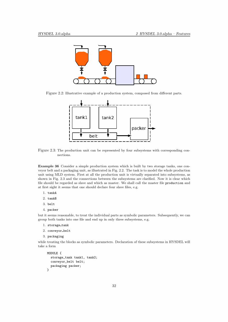
Figure 2.2: Illustrative example of a production system, composed from different parts.

Figure 2.3: The production unit can be represented by four subsystems with corresponding con-

nections.

Example 36 Consider a simple production system which is built by two storage tanks, one con-veyor belt and a packaging unit, as illustrated in Fig. 2.2. The task is to model the whole productionunit using MLD system. First at all the production unit is virtually separated into subsystems, asshown in Fig. 2.3 and the connections between the subsystems are clarified. Now it is clear whichfile should be regarded as slave and which as master. We shall call the master file production andat first sight it seems that one should declare four slave files, e.g.

1. tankA

2. tankB

3. belt

4. packer

but it seems reasonable, to treat the individual parts as symbolic parameters. Subsequently, we cangroup both tanks into one file and end up in only three subsystems, e.g.

1. storage tank

2. conveyor belt

3. packaging

while treating the blocks as symbolic parameters. Declaration of these subsystems in HYSDEL willtake a form

MODULE {


conveyor_belt belt;

packaging packer;

}

32


and it corresponds to three HYSDEL files which will be included, i.e.

1. storage tank.hys

2. conveyor belt.hys

3. packaging.hys

Each of these file is a slave file, structured without MODULE section. For instance, the filestorage tank.hys may be written in HYSDEL language as follows

SYSTEM storage_tank {

INTERFACE {

STATE { REAL level; }

INPUT { REAL u; }

OUTPUT { REAL y; }

PARAMETER {

REAL diameter;

REAL k=1e-2;

}

}

IMPLEMENTATION {

CONTINUOUS { level = level+1/diameter*(u-k*level);}

OUTPUT { y = level; }

}

}

Note that in this file some parameters are kept as symbolic and these values have to be set tonumerical values before compiling. If the slave files are defined, then we can define the INTERFACEpart of the master file as follows

INTERFACE {

MODULE {


conveyor_belt belt;

packaging packer;

}

STATE { REAL time [0, 1000]; }

INPUT { REAL raw_flow(2) [0, 5; 0, 5]; }

OUTPUT { REAL packages; }

PARAMETER {

tank1.diameter = 0.3;

tank2.diameter = 0.5;

belt.width = 1;

}

}

where the symbolic parameters are explicitly set. Moreover, the master file has two inputs raw flow,defined as vector, one state time, and one output called packages.

Merging – IMPLEMENTATION part

In the IMPLEMENTATION part it is required to specify connection between internal subsys-tems. This can be done in LINEAR section while keeping the standard syntax of linear item.The parameters of the slave files can be accessed like Matlab structures, as mentioned insection 2.2.4. The main change is that inputs will be referred with symbol u while outputswith symbol y as follows

33


par.u

.y

where par denotes the subsystem’s name.

Example 37 In this example we will return to example 36 and specify connections according thesketch Fig. 2.3. The IMPLEMENTATION section may be given as

IMPLEMENTATION {

LINEAR {

tank1.u = raw_flow(1);

tank2.u = raw_flow(2);

belt.u = tank1.y + tank2.y;

belt.y = packer.u;

}

CONTINUOUS {

time = time + 1;

}

OUTPUT {

packages = packer.y;

}

MUST {

tank1.level <= 1;

tank2.level <= 0.8;

}

}

where LINEAR section declares connections between subsystems. The section OUTPUT assigns thevariable packages to be output from packaging unit which is an overall output variable. Moreover,note that state update equation is also defined, as well as constraints.

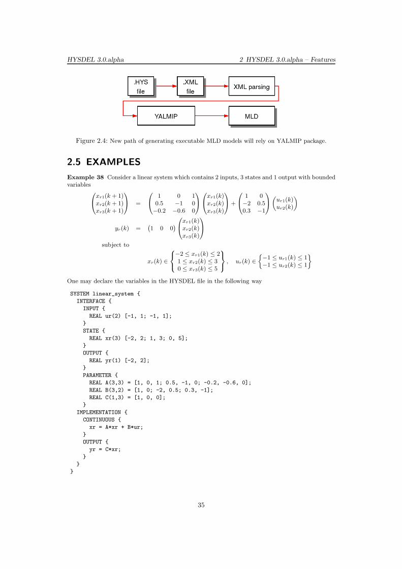
2.4 Implementation of new HYSDEL

Implementation of the HYSDEL 3.0.alpha will differ from the standard compilation proce-dure, as sketched in Fig. 1.1. The core will be replaced with YALMIP package [2] which hasmany advantages, namely

• direct handling of advanced syntax

• improved condition checking and merging features

• automatic model optimization.

Arising from this tool the compilation will be performed faster that standard HYSDELcompilator.

34


Figure 2.4: New path of generating executable MLD models will rely on YALMIP package.

2.5 EXAMPLES

Example 38 Consider a linear system which contains 2 inputs, 3 states and 1 output with boundedvariables

0

@

xr1(k + 1)xr2(k + 1)xr3(k + 1)

1

A =

0

@

1 0 10.5 −1 0−0.2 −0.6 0

1

A

0

@

xr1(k)xr2(k)xr3(k)

1

A +

0

@

1 0−2 0.50.3 −1

1

A

„

ur1(k)ur2(k)

«

yr(k) =`

1 0 0´

0

@

xr1(k)xr2(k)xr3(k)

1

A

subject to

xr(k) ∈

8

<

:

−2 ≤ xr1(k) ≤ 21 ≤ xr2(k) ≤ 30 ≤ xr3(k) ≤ 5

9

=

;

, ur(k) ∈

−1 ≤ ur1(k) ≤ 1−1 ≤ ur2(k) ≤ 1

ff

One may declare the variables in the HYSDEL file in the following way

SYSTEM linear_system {

INTERFACE {

INPUT {

REAL ur(2) [-1, 1; -1, 1];

}

STATE {

REAL xr(3) [-2, 2; 1, 3; 0, 5];

}

OUTPUT {

REAL yr(1) [-2, 2];

}

PARAMETER {

REAL A(3,3) = [1, 0, 1; 0.5, -1, 0; -0.2, -0.6, 0];

REAL B(3,2) = [1, 0; -2, 0.5; 0.3, -1];

REAL C(1,3) = [1, 0, 0];

}

IMPLEMENTATION {

CONTINUOUS {

xr = A*xr + B*ur;

}

OUTPUT {

yr = C*xr;

}

}

}

35

Bibliography

[1] A. Bemporad and M. Morari. Control of Systems Integrating Logic, Dynamics, andConstraints. Automatica, 35(3):407–427, March 1999.

[2] J. Lofberg. Yalmip : A toolbox for modeling and optimization in MATLAB. In Proceed-

ings of the CACSD Conference, Taipei, Taiwan, 2004.

36

Documents

Towards HYSDEL 3.0 - uiam.sk