Embed Size (px)
Citation preview
Diss. ETH No. 19344
Towards Many-Core Real-Time
Embedded Systems: Software Design of
Streaming Systems at System Level
A dissertation submitted to the
ETH ZURICH
for the degree of
Doctor of Sciences
presented by
KaiHuang
M.S. Computer ScienceLeiden University, the Netherland
born 02.10.1977citizen of China
accepted on the recommendation of
Prof. Dr. Lothar Thiele, examinerProf. Dr. Peter Marwedel, co-examiner
2010

Institut für Technische Informatik und KommunikationsnetzeComputer Engineering and Networks Laboratory
TIK-SCHRIFTENREIHE NR. 119
Kai Huang
Towards Many-Core Real-TimeEmbedded Systems: Software Design of
Streaming Systems at System Level
Eidgenössische Technische Hochschule ZürichSwiss Federal Institute of Technology Zurich
A dissertation submitted to theSwiss Federal Institute of Technology (ETH) Zürichfor the degree of Doctor of Sciences
Diss. ETH No. 19344
Prof. Dr. Lothar Thiele, examinerProf. Dr. Peter Marwedel, co-examiner
Examination date: 12. November, 2010
Abstract
Nowadays, multi-core architectures become popular for embeddedsystems. As VLSI technology is scaling to deep sub-micron domain,an envisioned trend is that the architectures of embedded systems aremoving from multiple cores to many cores. Although state-of-art multi-core and future many-core architectures provide enormous potential,scaling the number of computing cores does not directly translate intohigh performance and power efficiency. To exploit the potential of amulti(many)-core platform under stringent time-to-market constraints,software development does not only need to tackle the still-valid classicalrequirements, e.g., memory constraints, programming heterogeneity, andreal-time responsiveness, but also face new challenges stemming fromthe increasing number of computing cores, for instance, scalability of thetechnologies.
In this thesis, we focus on the class of streaming embedded systemsat system level and address three important aspects of the softwareconstruction of multi/many-core embedded systems, i. e. , programming,performance, and power. To address the programmability ofmulti/many-core embedded systems, we present a model-of-computation basedprogrammingmodelwhich supports scalable specifications of a system ina parametrized manner. In terms of performance estimation, we presentboth analytic and simulation-based techniques to tackle the complexinterference and correlations within multi/many-core embedded systemssuch that accurate estimation can be conducted. We also investigatepower-efficient design and propose offline and online algorithms fordynamic power management to reduce the static power consumptionunder hard real-time constraints.

Zusammenfassung
Mehrkernprozessoren werden bereits heute für eingebettete Systemeverwendet. Durch die weitere Miniaturisierung im SubmikrometerBereich ist zu erwarten, dass zukünftige Architekturen für eingebetteteSysteme auf Vielkernprozessoren anstatt Mehrkernprozessorenbasieren werden. Obwohl Mehrkernprozessoren und zukünftigeVielkernprozessoren enorme Möglichkeiten bieten, führt die steigendeAnzahl von Rechenkernen nicht direkt zu höherer Rechenleistungoder Energieeffizienz. Um die Möglichkeiten dieser Architekturen beikurzen Produktentwicklungszeiten ausschöpfen zu können, müssendaher bei der Softwareentwicklung sowohl bereits bekannte alsauch neue Aspekte berücksichtigt werden. Während beispielsweiseSpeichereinschränkungen, Heterogenität bei der Programmierung oderEchtzeitanforderungen weiterhin eine wichtige Rolle spielen, müssenzusätzlich die Skalierbarkeit bezüglich der Anzahl der Prozessorkerneoder technologische Einschränkungen bei der Softwareentwicklungbeachtet werden.
In der vorliegenden Dissertation liegt der Schwerpunkt auf einge-betteten Systemen für Streaming Anwendungen, wobei drei Aspekteder Softwareentwicklung näher betrachtet werden: Programmierung,Analyse des Zeitverhaltens und Leistungsaufnahme. Zur Program-mierung von eingebetteten Systemen mit Mehr-/Vielkernprozessorenwird ein Programmiermodell vorgestellt, das die skalierbare Spezifika-tion eines Systems in parametrisierter Form ermöglicht. Zur Analysedes Zeitverhaltenswerden analytische und simulationsbasierte Verfahrenvorgestellt, welche zur Erzielung genauer Resultate die kompliziertenzeitlichen Interferenzen undKorrelationen inMehr-/Vielkernprozessorenberücksichtigen. Schliesslich wird der Entwurf von Systemen miteffizienter Leistungsaufnahme betrachtet, wobei online und offlineAlgorithmen vorgestellt werden, um den statischen Leistungsverbrauchunter harten Echtzeitbedingungen zu reduzieren.


Acknowledgement
First of all, I would like to expressmy sincere gratitude to Prof. Dr. LotharThiele for offering the opportunity for a PhD and constantly patientlysupervisingmy research. Without his support, this thesis would have notbeen possible.
I would like to thank Prof. Dr. Peter Marwedel for being my co-examiner in this thesis.
I would also like to thank: Prof. Dr. Jian-jia Chen and Prof. Dr.Giorgio C. Buttazzo for the fruitful research cooperation; Dr. AlexanderMaxiaguine and Dr. Simon Künzli for their valuable suggestions andhelp in the beginning of my PhD life; Dr. Wolfgang Haid for the nicecollaboration in the four-year SHAPES project and for taking his time ofproofreading my thesis, and Dr. Iuliana Bacivarov and Luca Santinellifor nice research cooperation. Furthermore, I would like to thank all myformer and current colleagues of the whole TEC group for their companyand support, especially Dr. Clemens Moser for the great time we hadwhile sharing our office for more than four years.
Finally, my dearest thanks go to my family for their love and supportthroughout all these years of my PhD study.
The work presented in this thesis was supported by the EuropeanIntegrated Project SHAPES (grant no. 26825) under IST FET – AdvancedComputing Architecture (ACA). This support is gratefully acknowl-edged.

vi Acknowledgement

vii
To my wife, Yu, andto my daughter, Wei-yi.

viii Acknowledgement
Contents
Abstract i
Zusammenfassung iii
Acknowledgement v
1 Introduction 1
1.1 Multi-Core Embedded Systems . . . . . . . . . . . . . . . . 11.2 System Software Design . . . . . . . . . . . . . . . . . . . . 41.3 Thesis Outline and Contributions . . . . . . . . . . . . . . . 7
2 Programming Model 11
2.1 Overview . . . . . . . . . . . . . . . . . . . . . . . . . . . . . 122.2 Related Work . . . . . . . . . . . . . . . . . . . . . . . . . . 132.3 Kahn Process Network . . . . . . . . . . . . . . . . . . . . . 162.4 Syntax of Programming Model . . . . . . . . . . . . . . . . 17
2.4.1 Basic Principles . . . . . . . . . . . . . . . . . . . . . 172.4.2 Application Specification . . . . . . . . . . . . . . . 182.4.3 Architecture Specification . . . . . . . . . . . . . . . 232.4.4 Mapping Specification . . . . . . . . . . . . . . . . . 242.4.5 Experimental Results . . . . . . . . . . . . . . . . . . 25
2.5 Windowed-FIFO Communication . . . . . . . . . . . . . . . 272.5.1 Motivation . . . . . . . . . . . . . . . . . . . . . . . . 272.5.2 Semantics and Syntax . . . . . . . . . . . . . . . . . 292.5.3 Properties . . . . . . . . . . . . . . . . . . . . . . . . 312.5.4 Implementation Issues . . . . . . . . . . . . . . . . . 332.5.5 Empirical Case Studies . . . . . . . . . . . . . . . . . 34
2.6 Parallel SystemC Functional Simulation . . . . . . . . . . . 372.6.1 Simulation Framework Overview . . . . . . . . . . 382.6.2 SystemC Introduction . . . . . . . . . . . . . . . . . 392.6.3 Stand-alone SystemC Functional Simulation . . . . 412.6.4 Parallel SystemC Simulation . . . . . . . . . . . . . 412.6.5 Experimental Results . . . . . . . . . . . . . . . . . . 45
x Contents
2.7 Summary . . . . . . . . . . . . . . . . . . . . . . . . . . . . . 47
3 Performance Evaluation 49
3.1 Overview . . . . . . . . . . . . . . . . . . . . . . . . . . . . . 503.2 Modular Performance Analysis . . . . . . . . . . . . . . . . 51
3.2.1 Related Work . . . . . . . . . . . . . . . . . . . . . . 523.2.2 Introduction to Rtc-mpa . . . . . . . . . . . . . . . . 543.2.3 Analysis of Correlated Streams . . . . . . . . . . . . 573.2.4 Experimental Results . . . . . . . . . . . . . . . . . . 65
3.3 Trace-Based Simulation . . . . . . . . . . . . . . . . . . . . . 713.3.1 Related Work . . . . . . . . . . . . . . . . . . . . . . 713.3.2 Modeling . . . . . . . . . . . . . . . . . . . . . . . . 733.3.3 Simulation Framework . . . . . . . . . . . . . . . . . 773.3.4 Experimental Results . . . . . . . . . . . . . . . . . . 84
3.4 Summary . . . . . . . . . . . . . . . . . . . . . . . . . . . . . 87
4 Power Management 89
4.1 Overview . . . . . . . . . . . . . . . . . . . . . . . . . . . . . 904.2 Related Work . . . . . . . . . . . . . . . . . . . . . . . . . . 914.3 System Model and Problem Definition . . . . . . . . . . . . 93
4.3.1 System Model . . . . . . . . . . . . . . . . . . . . . . 934.3.2 Worst-Case Interval-Based Streaming Model . . . . 944.3.3 Problem Definition . . . . . . . . . . . . . . . . . . . 95
4.4 Real-Time Calculus Routines . . . . . . . . . . . . . . . . . 964.4.1 Bounded Delay . . . . . . . . . . . . . . . . . . . . . 964.4.2 Future Prediction with Historical Information . . . 984.4.3 Backlogged Demand . . . . . . . . . . . . . . . . . . 99
4.5 Online DPM for Single Stream . . . . . . . . . . . . . . . . . 1004.5.1 Deactivation Algorithm . . . . . . . . . . . . . . . . 1014.5.2 Activation Algorithms . . . . . . . . . . . . . . . . . 1024.5.3 Experimental Results . . . . . . . . . . . . . . . . . . 109
4.6 Online DPM for Multiple Streams . . . . . . . . . . . . . . 1134.6.1 FP Scheduling with Individual Backlog . . . . . . . 1134.6.2 EDF Scheduling with Individual Backlog . . . . . . 1154.6.3 EDF Scheduling with Global Backlog . . . . . . . . 1164.6.4 Experimental Results . . . . . . . . . . . . . . . . . . 118
4.7 Offline Periodic DPM . . . . . . . . . . . . . . . . . . . . . . 1214.7.1 System Model and Problem Definition . . . . . . . . 1214.7.2 Motivational Example . . . . . . . . . . . . . . . . . 1234.7.3 Bounded Delay Approximation . . . . . . . . . . . . 1234.7.4 Experimental Results . . . . . . . . . . . . . . . . . . 129
4.8 Summary . . . . . . . . . . . . . . . . . . . . . . . . . . . . . 131

Contents xi
5 Conclusions 1335.1 Main Results . . . . . . . . . . . . . . . . . . . . . . . . . . . 1335.2 Future Perspectives . . . . . . . . . . . . . . . . . . . . . . . 134
Bibliography 137
List of Publications 153
Curriculum Vitae 157

xii Contents

1Introduction
Multi-core architectures are widely used for embedded systems nowa-days. The number of computing cores is keeping on increasing as VLSItechnology is scaling to deep sub-micron domain. An envisioned trendis that embedded systems are moving frommultiple cores to many cores.This thesis presents a set of novel techniques for contemporary multi-core and future many-core embedded system design. In particular, wefocus on solutions for the new challenges imposed by CMOS technologyscaling. Section 1.1 and 1.2 survey the state-of-art platforms and softwaretool flows for multi-core embedded systems, respectively. Section 1.3draws the outline and summarizes the contributions of this thesis.
1.1 Multi-Core Embedded Systems
Modern embedded systems require massive computational power dueto computationally intensive embedded applications, e.g., real-timespeech recognition, video conferencing, software-defined radio, andcryptography. An embedded system running all these applicationsdemands a total performance payload of up to 10, 000 SPECInt benchmarkunits [ABM+04]. The situation will become even worse since the demandfor computation will further grow. Future embedded applications likeembedded computer vision [KBC09], for instance, require computationalpower far beyondwhat can be provided by state-of-art embedded systemarchitectures [WJM08].
Besides the computational demand, power consumption is another
2 Chapter 1. Introduction
first-class design concern for embedded systems. A major category ofembedded systems, for instance, are hand-held mobile devices whichare powered by batteries. The batteries for such devices are limitedin both power and energy output. The amount of energy availablethus severely limits a system’s lifespan. Although research continuesto develop batteries with higher energy-density, the slow growth of theenergy density of batteries lags far behind the tremendous increase ofdemands [ITR].
To copewith the ever increasingdemandof computation and stringentpower constraints ofmodern embedded systems,multi-core architecturesbecome the de facto choice. These are two driving forces to usemulti-corearchitectures: On the one hand, CMOS circuits advance to the deep sub-micro domain, which will aid sustaining Moore’s law in the future – thenumber of transistors within a chip doubles every 18 months. A recentevidence, for instance, is the newly unveiled Intel Single-chip CloudComputer (SCC) [SCC] which integrates 1.3 billion transistors within 567square millimeters manufactured using a 45 nm CMOS High-K metalgate process. On the other hand, increasing clock frequencies and deeperpipelines cannot sustain the performance increase under constraints ofpower consumption and thermal dissipation, i.e., hitting the powerwall [PH09]. Experience suggests that performance only doubles withquadrupled complexity of a chip [Bor07].
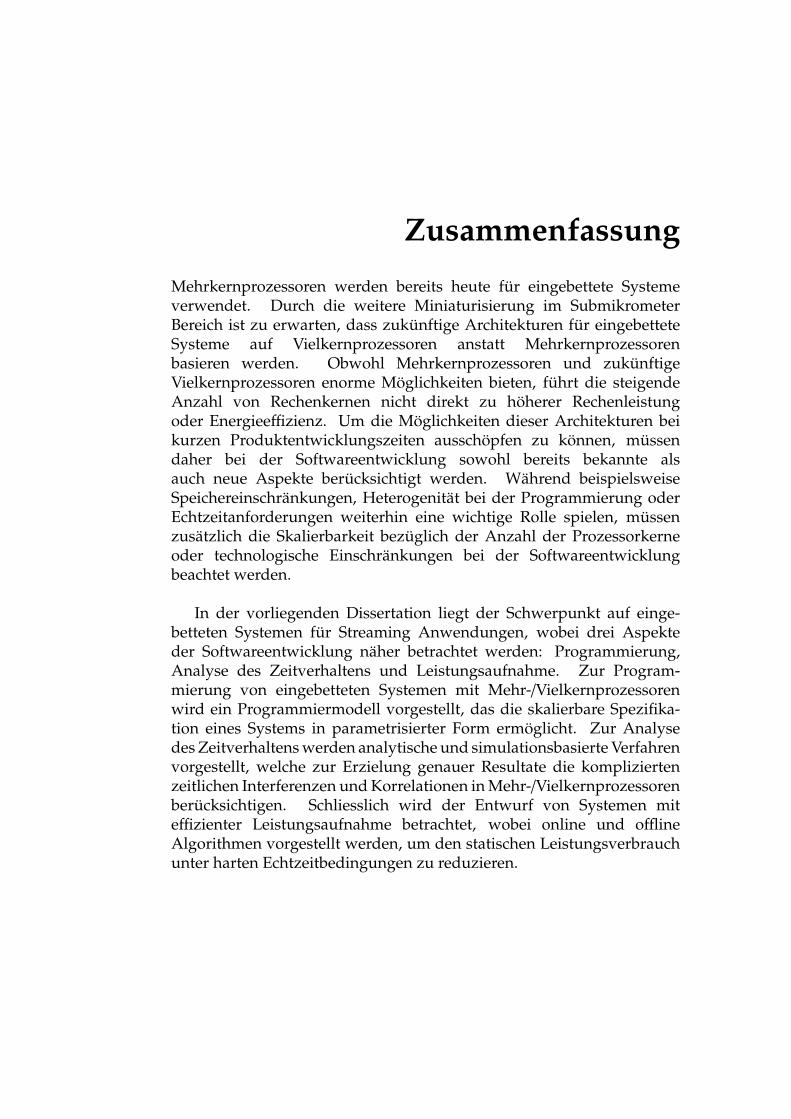
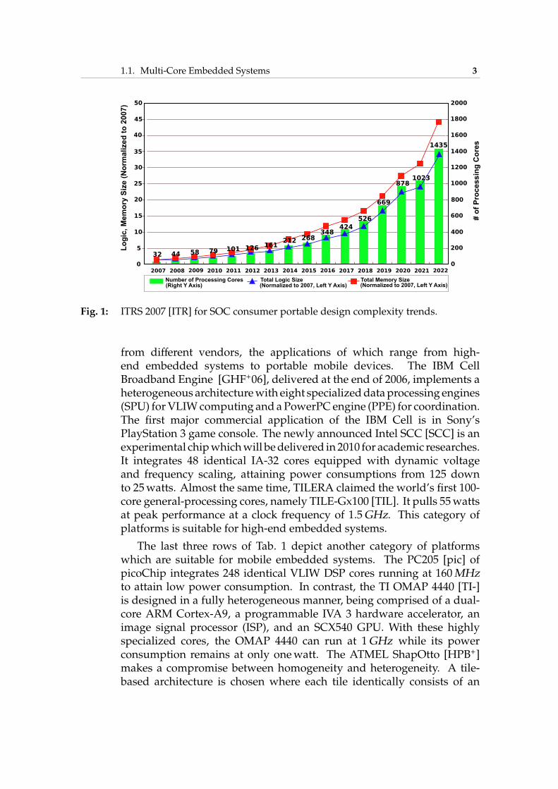
The main advantage of multi-core architectures is that raw per-formance increases can be accomplished by increasing the number ofcomputing cores rather than frequency, which translates into a slowergrowth in power consumption. For a given processor architecture ina given technology, under-clocking with lower supply voltage decreasespower consumptionmuchmore thanperformance. On the other hand, forthe samepower consumption, a dual-core solution clocked at a 20% lowerfrequency would bring in theory 73% more performance than a singlecore [CCBB09]. Therefore, multi-core architectures embody a good trade-off between technology scaling and strict power budget requirements.Consequently, ITRS predicts that by the end of the decade consumerportable Systems-on-Chip (SoC) will contain more than 1, 400 cores, asdepicted in Fig. 1. Multi-core embedded systems are inevitably evolvingto many-core embedded systems. In the rest of this section, we surveya few prominent cutting-edge multi-core embedded system platforms,some of which actually have many cores.
Multi-core architectures have a longer history in embedded systemsthan in desktop commercial products because embedded systems hitthe power wall earlier [WJM08]. One of the first commercial multi-coreplatforms, the Lucent Daytona [AAB+00], for instance, wasmanufactureda decade ago. Tab. 1 lists six state-of-art multi/many-core platforms
1.1. Multi-Core Embedded Systems 3
1435
2000
1800
1600
1400
1200
1000
800
600
400
200
02022202120202019201820172016201520142013201220112010200920082007
0
5
10
15
20
25
30
35
40
45
50
# o
f P
roce
ss
ing
Co
res
Lo
gic
, M
em
ory
Siz
e (
No
rmalize
d t
o 2
00
7)
32 44 58
1023878
669
526
424348
26821216112610179
Number of Processing Cores(Right Y Axis)
Total Logic Size(Normalized to 2007, Left Y Axis)
Total Memory Size(Normalized to 2007, Left Y Axis)
Fig. 1: ITRS 2007 [ITR] for SOC consumer portable design complexity trends.
from different vendors, the applications of which range from high-end embedded systems to portable mobile devices. The IBM CellBroadband Engine [GHF+06], delivered at the end of 2006, implements aheterogeneous architecturewith eight specializeddataprocessing engines(SPU) forVLIWcomputing and aPowerPC engine (PPE) for coordination.The first major commercial application of the IBM Cell is in Sony’sPlayStation 3 game console. The newly announced Intel SCC [SCC] is anexperimental chipwhichwill bedelivered in 2010 for academic researches.It integrates 48 identical IA-32 cores equipped with dynamic voltageand frequency scaling, attaining power consumptions from 125 downto 25watts. Almost the same time, TILERA claimed the world’s first 100-core general-processing cores, namely TILE-Gx100 [TIL]. It pulls 55wattsat peak performance at a clock frequency of 1.5GHz. This category ofplatforms is suitable for high-end embedded systems.
The last three rows of Tab. 1 depict another category of platformswhich are suitable for mobile embedded systems. The PC205 [pic] ofpicoChip integrates 248 identical VLIW DSP cores running at 160MHzto attain low power consumption. In contrast, the TI OMAP 4440 [TI-]is designed in a fully heterogeneous manner, being comprised of a dual-core ARM Cortex-A9, a programmable IVA 3 hardware accelerator, animage signal processor (ISP), and an SCX540 GPU. With these highlyspecialized cores, the OMAP 4440 can run at 1GHz while its powerconsumption remains at only onewatt. The ATMEL ShapOtto [HPB+]makes a compromise between homogeneity and heterogeneity. A tile-based architecture is chosen where each tile identically consists of an
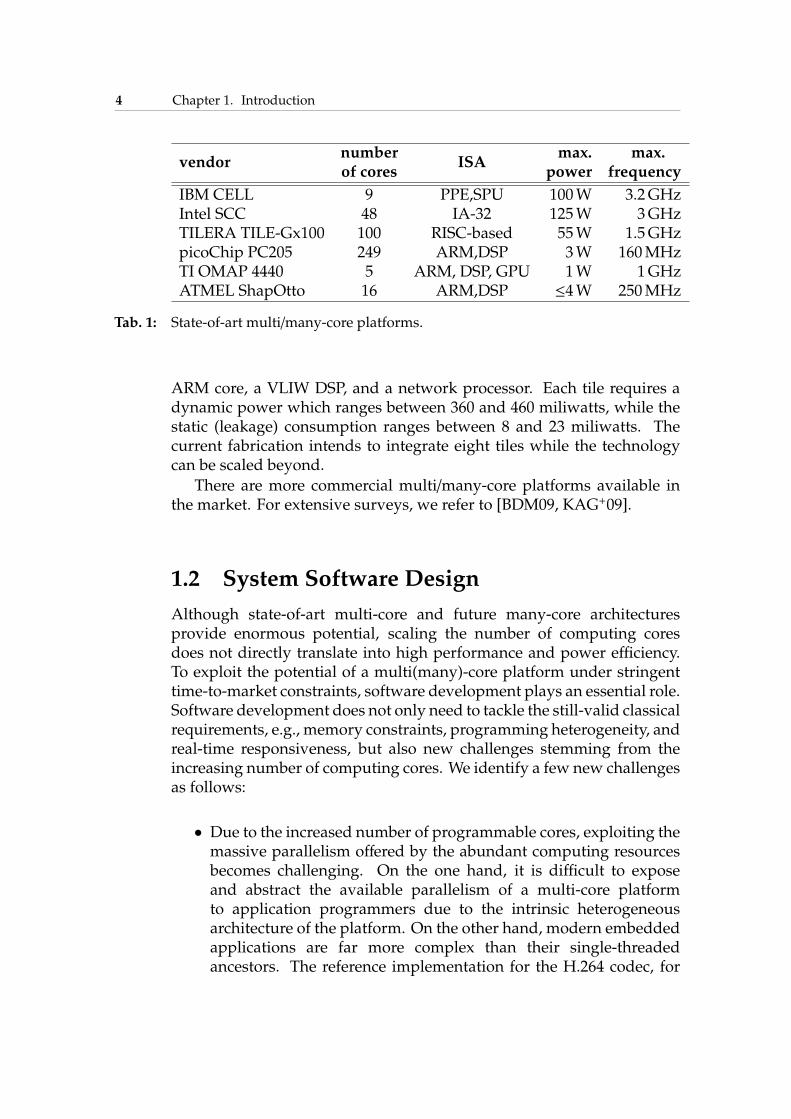
4 Chapter 1. Introduction
vendornumber
ISAmax. max.
of cores power frequency
IBM CELL 9 PPE,SPU 100W 3.2GHzIntel SCC 48 IA-32 125W 3GHzTILERA TILE-Gx100 100 RISC-based 55W 1.5GHzpicoChip PC205 249 ARM,DSP 3W 160MHzTI OMAP 4440 5 ARM, DSP, GPU 1W 1GHzATMEL ShapOtto 16 ARM,DSP ≤4W 250MHz
Tab. 1: State-of-art multi/many-core platforms.
ARM core, a VLIW DSP, and a network processor. Each tile requires adynamic power which ranges between 360 and 460 miliwatts, while thestatic (leakage) consumption ranges between 8 and 23 miliwatts. Thecurrent fabrication intends to integrate eight tiles while the technologycan be scaled beyond.
There are more commercial multi/many-core platforms available inthe market. For extensive surveys, we refer to [BDM09, KAG+09].
1.2 System Software Design
Although state-of-art multi-core and future many-core architecturesprovide enormous potential, scaling the number of computing coresdoes not directly translate into high performance and power efficiency.To exploit the potential of a multi(many)-core platform under stringenttime-to-market constraints, software development plays an essential role.Software development does not only need to tackle the still-valid classicalrequirements, e.g., memory constraints, programming heterogeneity, andreal-time responsiveness, but also new challenges stemming from theincreasing number of computing cores. We identify a few new challengesas follows:
• Due to the increased number of programmable cores, exploiting themassive parallelism offered by the abundant computing resourcesbecomes challenging. On the one hand, it is difficult to exposeand abstract the available parallelism of a multi-core platformto application programmers due to the intrinsic heterogeneousarchitecture of the platform. On the other hand, modern embeddedapplications are far more complex than their single-threadedancestors. The reference implementation for the H.264 codec, for
1.2. System Software Design 5
instance, consists of over 120, 000 lines of C code. Parallelizing it isa tedious and error-prone process. The questions are:
How to efficiently program an multi/many-core platform with respect toboth performance and time-to-market? Can such a programming modelscale to future many-core platforms?
• The increased number of computing cores would lead to average-case performance gains, whereas the worst-case performancemight decrease because of complex interactions within a system.Furthermore, even the average case is difficult to measure becauseof the intrinsic heterogeneity of modern multi-core platforms. Thetraditional cycle/instruction-accurate simulation techniques are fartoo slow. The question here is:
How to estimate the performance of large multi/many-core embeddedsystems with reasonable time and accuracy?
• The tremendous amount of integrated transistors within a chipincurs a new power-efficiency problem, i.e., static power consump-tion caused by leakage current. The leakage current originates inthe dramatic increase in both sub-threshold current and gate-oxideleakage current, which is projected to account for as much as 50percent of the total power dissipation for high-end processors in 90-nm technology [ABM+04]. The ITRS expects the static powerwill bemuch greater than its predictions due to variability and temperatureeffects [ITR]. The question hereby is:
How to effectively reduce the static power under real-time constraints?
This thesis aims to give partial answers to these new challengesimposed by the steadily increasing number of programming cores ofmodern multi-core and future many-core embedded systems. Beforepresenting our contributions, we review the state-of-art related workin the literature. Due to the vast amount of related work, onlya representative subset is discussed with an emphasis on multi-coreembedded systems. For extensive surveys, we refer to [MJU+09,HHBT09a, wPOH09, KB09].
To the first category belong compiler-based approaches where aconventional sequential language like C is used as an initial specificationfor applications and the compiler automatically extracts parallelism fromthe sequential representation. Example frameworks are MAPS [CCS+08],Compaan [SZT+04], and CriticalBlue multi-core Cascade [Cri]. Thisapproach is appreciated by application programmers because the com-plicated parallelism extraction is transparent and does not impose any
6 Chapter 1. Introduction
burden on the programmers. Automated parallelization, however, ischallenging and effective parallelism extraction is rather cumbersomewithout domain-specific knowledge. Therefore, compiler-based ap-proaches are normally limited to applications with evident data-parallelregions or with relatively static behavior.
To ease the job of compilers, one widely adopted approach is to use anexplicit application programming interface (API) during the applicationdevelopment. Using APIs, application programmers can make use oftheir domain-specific knowledge, e.g., identifying the parallel regions,and give hints to the compiler for better parallelization. Well-knownAPIs are OpenMP [Ope] for shared-memory architectures, MPI [MPI] fordistributed-memory architectures, and TTL [vdWdKH+04] for high-levelabstraction. Industrial chip vendors adopt this approach widely withintheir software development kits. CUDA [BFH+04, ati] from NVIDIA andBrook+ [CUD] from AMD ATI are parallel programming solutions forGPUs, which provide specific APIs to manipulate the GPU memory andto express single-instruction multiple-data (SIMD) data parallelism. TheAPI-based approach allows better low-level control of the parallelismby the programmer and, therefore, promises better performance if theAPIs are properly used. The major drawback of compiler/API-basedapproaches is that an application can be written in an arbitrary form,consequently complicating quantitative analysis.
Model-driven development is recently advocated as a viable alterna-tive. By restricting an application to a certain model of computation,quantitative analysis with respect to e.g. schedulability tests andworst-case behavior can be tackled in a reasonable manner. A well-known model-of-computation is the Kahn process network [Kah74]where an application is composed of autonomous processes whichcommunicate asynchronously via point-to-point FIFO channels. Designflows based on Kpn are e.g. Koski [KKO+06], DOL [TBHH07],SESAME/DAEDALUS [PEP06, NSD08]. Another widely used model-of-computation is the synchronous data flow (SDF) [LM87] which is arestricted version of Kpn. The SDF model enables static schedulinganalysis at compile time, which provides guarantees on, for instance,finite size of communication buffers and deadlock-free execution. Toolflows adopting the SDF are, for instance, SHIM [ET06], PEACE [HKL+07],and StreamIt [TKA02]. There are other frameworks supporting multiplemodels-of-computation simultaneously. For instance, Ptolemy [pto]supports heterogeneous modeling and Metropolis [BWH+03] defines ameta-model that can be refined into a specific model-of-computation. Tocompare different models-of-computation, E. Lee and A. S. Vincentellipresent a framework [LSV98]. An overview of applying models-of-computation in system design is presented in [ELLSV97].
1.3. Thesis Outline and Contributions 7
Although a vast amount of research effort has been devoted into thisfield, the aforementioned challenges are not completely solved. Thedeveloped techniques are not well suited for futuremany-core embeddedsystems, which motivates our work. In this thesis, we try to tacklethese challenges for both contemporary multi-core and future many-coreembedded systems, in particular for a specific application domain.
1.3 Thesis Outline and Contributions
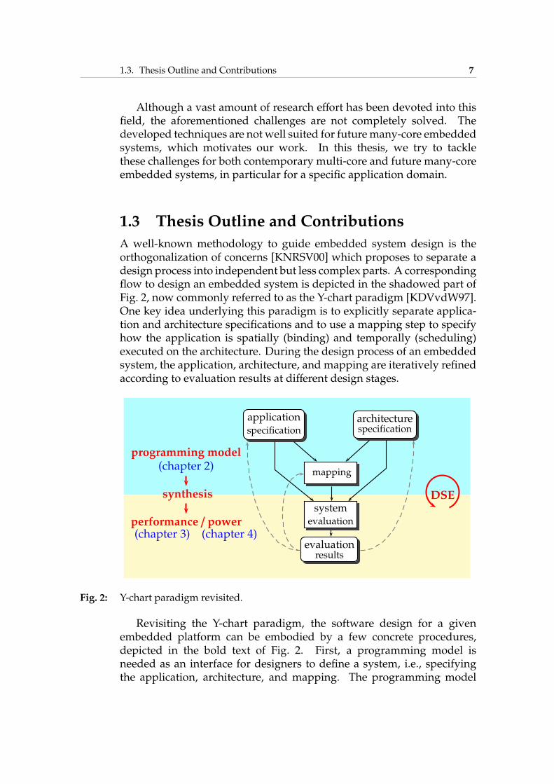
A well-known methodology to guide embedded system design is theorthogonalization of concerns [KNRSV00] which proposes to separate adesign process into independent but less complex parts. A correspondingflow to design an embedded system is depicted in the shadowed part ofFig. 2, now commonly referred to as the Y-chart paradigm [KDVvdW97].One key idea underlying this paradigm is to explicitly separate applica-tion and architecture specifications and to use a mapping step to specifyhow the application is spatially (binding) and temporally (scheduling)executed on the architecture. During the design process of an embeddedsystem, the application, architecture, and mapping are iteratively refinedaccording to evaluation results at different design stages.
applicationspecification
architecturespecification
mapping
systemevaluation
evaluationresults
programming model(chapter 2)
synthesis
performance / power(chapter 3) (chapter 4)
DSE
Fig. 2: Y-chart paradigm revisited.
Revisiting the Y-chart paradigm, the software design for a givenembedded platform can be embodied by a few concrete procedures,depicted in the bold text of Fig. 2. First, a programming model isneeded as an interface for designers to define a system, i.e., specifyingthe application, architecture, and mapping. The programming model

8 Chapter 1. Introduction
defineswhichmodel-of-computation to use and the programming syntaxof the specifications. Second, to evaluate a candidate design, metrics andthe corresponding evaluation model need to be defined. To analyticallyevaluate the performance of a system, for instance, a formal performancemodel for the system is needed. In addition, the programming modeland the evaluation model are normally defined at different levels ofabstraction. An automated synthesis is preferable to refine a systemfrom one level of abstraction to the next in a correct manner in terms offunctional and possibly non-functional properties. Last but not least, adesign space exploration (DSE) procedure is also desirable in order tofind the optimal design in a systematic and automated manner.
None of the procedures in the Y-chart paradigm is trivial. In thisthesis, we target the domain of streaming applications and provide aset of novel techniques for the software construction for contemporarymulti-core and future many-core embedded systems, trying to tackle theaforementioned design challenges. We demonstrate on the one hand howthe aforementioned challenges can be tackled in a systematic manner, onthe other hand the proposed solutions can be smoothly unified in a samesoftware framework for the assessment of system-level design decisions.Specifically, we focus on the programming model (chapter 2) and twodifferent metrics, i.e., performance (chapter 3) and energy (chapter 4), asdepicted in Fig. 2. For automated software synthesis and design spaceexploration, we refer to [HKH+09, Hai10] and [Gri04, Kü06], respectively.The major contributions of the thesis are summarized as follows:
Chapter 2: Programming Model
In Chapter 2, we present a programming model based on Kpn. Ourprogrammingmodel separates the application, architecture, andmappingspecifications of a system. For application modeling, the Kpn model-of-computation is strictly adhered. To avoid the costly communication andsynchronization overheads incurred by large scale process networks, theFIFO syntax of a Kpn is extended by a so-called windowed FIFO. We alsodevelop a distributed functional simulation as a proof-of-concept runtimeenvironment for our programmingmodel. The detailed contributions arelisted in the following:
• Following the orthogonalization-of-concerns methodology, we con-struct the syntax of our programming model. We define XMLschemata for the system specifications, i.e., the structure of theapplication, the abstract architecture, and the mapping. To assistthe design of large systems, a so-called iterator is developed bywhich a system can be arbitrarily scaled in a parametrized manner.We also define a set of C/C++ coding rules for the specification of
1.3. Thesis Outline and Contributions 9
the functionality of individual processes in an application processnetwork, To reduce theworkloads of application programmers, Ourcoding rules enable the reuse of a same piece of source code for aset of iterated processes.
• We propose a syntactical extension for the FIFO communication ofKpn, namely windowed-FIFO. We prove the syntactic coherency ofa windowed-FIFO process network to a standard Kpn. To validatethis concept, we develop a hardware implementation as well as theapplication software interface based on Xilinx FPGAs.
• To show the effectiveness of our programmingmodel, we develop aSystemC-based functional simulation as a runtime environment.To parallelize SystemC execution, we develop a library whichenables a concurrent execution of multiple SystemC kernels. Usingthis library, a functional simulation of an application can executeon an arbitrary number of Linux hosts connected via TCP/IP.Furthermore, the source code for the runtime environment canbe automatically generated from system specifications using ourprogramming model.
Chapter 3: Performance Estimation
InChapter 3, we consider the performancemetric in theY-chart paradigm.We investigate two techniques, i.e., an analytic method and a simulation-based approach, for worst and average case performance evaluation ofan sysetm at system level. For the formal method, we apply real-timecalculus [TCN00, CKT03] and develop new techniques for the analysisfor data stream correlations, which is typical for Kpn applications. For thesimulation-based approach, we develop a trace-based framework whichserves as a non-functional back-end of our programming model. Theproposed framework can estimate the performance of large streamingmulti/many-core systems within a reasonable time span with highaccuracy. Specifically, the detailed contributions are listed below:
• We investigate correlations of data streams within a fork-joinscenario in a Kpn network and present a method to analyze suchcorrelations based on different types of delays, e.g., splitting delayat the fork process and blocking delay at the join process. We showthe applicability of the presented methods by analyzing a concretemultimedia application.
• We propose a trace-based framework to simulate timing behaviorof multi/many-core embedded systems specified in aforementioned
10 Chapter 1. Introduction
programming model. By abstracting an application as coarse-grain traces, our framework can effectively and efficiently simulatecomplex systems, while considering different aspects pertaining toresource sharing, memory allocations, and multi-hop communica-tions. Wevalidate our framework bymapping anMPEG-2decodingalgorithm onto the ATMEL Diopsis-940 platform [Pao06]. We alsodemonstrate the scalability of our approach by simulating a scaledversion of the MPEG-2 algorithm on 16-core platform.
Chapter 4: Power Management
Chapter 4 explores system-level dynamic power management to reducestatic power consumption under real-time constraints. TheKpnmodelingof an application enables such an exploration at the same system level as tothe performance metric. For simplicity, we consider a dual-core scenario,i.e., a processing core for data stream processing and a control core forcoordination, for instance, to schedule the processing core. We proposeboth online and offline algorithms. To guarantee real-time requirements,We apply real-time calculus to predict future event arrivals and Real-Time Interface theory [TWS06] for the schedulability analysis. Basedon the adopted worst-case interval-based abstraction, our algorithmscannot only tackle arbitrary event arrivals (even with burstiness) butalso guarantee hard real-time constraints with respect to both timing andbacklog constraints. The contributions of this chapter are as follows:
• We formulate the problem of finding a periodic powermanagementscheme tominimize the average standby power consumption underhard real-time constraints. We provide optimal and approximatedoffline solutions for this problem. The light run-time overhead ofthe periodic power management scheme is particularly suitable forembedded systems with very limited power budgets.
• Alternatively, we propose online algorithms to reduce standbypower consumption. Our online algorithms adaptively predict thenextmode-switchmoment by considering both historical and futureevent arrivals, and procrastinate the buffered and future events aslate as possible.
• To handle multiple event streams with different characteristics,we develop solutions for two preemptive scheduling policies, i.e.,earliest-deadline-first and fixed priority, for resource sharing. Withrespect to system backlog organization, two different scenarios, i.e.,distributed and global backlog, are considered.
2Programming Model
The multi-core architectures of modern embedded platforms are highlyconcurrent and software-programmable. To exploit the available concur-rency and programmability, a multi-core platform has to be abstracted ata level where application programmers can efficiently develop softwarewithout digging deep into intricate hardware details. A programmingmodel is such an abstract representation. It defines an interface by whichapplication programmers specify an application and describe how theapplication runs on top of a platform. Reviewing Fig. 2, a programmingmodel is the starting point of the software development of an embeddedsystem. Besides the specification of a system, a programming model alsoaffects other procedures of the software construction, for instance, thewayhow system performance is evaluated and how design space explorationis conducted.
The highly concurrent and software-programmable nature of multi-core platforms does not directly translate into high performance andpower efficiency of a system. On the one hand, due to the heterogeneousarchitecture of multi-core platforms, it is difficult to expose and abstractthe availableparallelism in amulti-coreplatform in auniformand scalablemanner. On the other hand, an application needs to be parallelizedinto coarse-grained concurrent tasks to make use of the computing cores.However, modern embedded applications are far more complex thantheir single-threaded ancestors. The reference implementation for theH.264 video codec, for instance, consists of over 120, 000 lines of C code.Parallelizing an applicationwith such a complexity is a tedious and error-prone process. Furthermore, the performance gains obtained through
12 Chapter 2. Programming Model
this coarse-grained parallelization could be overshadowed by the costof communication and synchronization overhead among the partitionedconcurrent tasks. This effect will be accentuated as more computationalcores are integrated and finer-granularity tasks are partitioned.
The questions to answer are: How can a multi-core platform beefficiently programmed with respect to both performance and time-to-market? Can such a programming model scale to future many-coreplatforms?
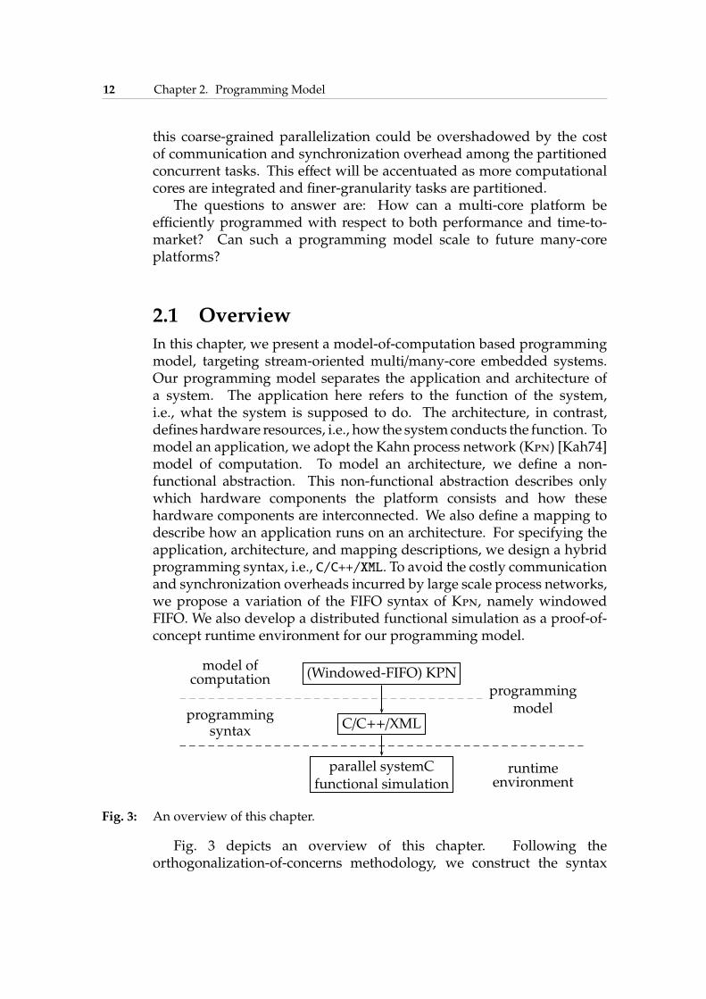
2.1 Overview
In this chapter, we present a model-of-computation based programmingmodel, targeting stream-oriented multi/many-core embedded systems.Our programming model separates the application and architecture ofa system. The application here refers to the function of the system,i.e., what the system is supposed to do. The architecture, in contrast,defines hardware resources, i.e., how the systemconducts the function. Tomodel an application, we adopt the Kahn process network (Kpn) [Kah74]model of computation. To model an architecture, we define a non-functional abstraction. This non-functional abstraction describes onlywhich hardware components the platform consists and how thesehardware components are interconnected. We also define a mapping todescribe how an application runs on an architecture. For specifying theapplication, architecture, and mapping descriptions, we design a hybridprogramming syntax, i.e., C/C++/XML. To avoid the costly communicationand synchronization overheads incurred by large scale process networks,we propose a variation of the FIFO syntax of Kpn, namely windowedFIFO. We also develop a distributed functional simulation as a proof-of-concept runtime environment for our programming model.
(Windowed-FIFO) KPN
C/C++/XML
parallel systemCfunctional simulation
model ofcomputation
programmingsyntax
runtimeenvironment
programmingmodel
Fig. 3: An overview of this chapter.
Fig. 3 depicts an overview of this chapter. Following theorthogonalization-of-concerns methodology, we construct the syntax
2.2. Related Work 13
of our programming model. We define XML schemata for systemspecifications, i.e., the structure of the application process network, theabstract architecture, and the mapping. To assist the design of largesystems, a so-called iterator is developed by which a system can bearbitrarily scaled in a parametrized manner. We also define a set ofC/C++ coding rules for the specification of the functionality of individualprocesses in an application process network. To reduce the workload ofapplication programmers, our coding rules enable the reuse of the samepiece of source code for a set of iterated processes. We propose a syntacticvariation for the FIFO communication of Kpn, namely windowed-FIFO.We prove the syntactic coherency of a windowed-FIFO process networkto a standard Kpn. To validate this concept, we also develop a hardwareIP based on Xilinx FPGAs.
To functionally verify an application specified in our programmingmodel, we develop a SystemC-based functional simulation, which servesas a prototype runtime environment. To efficiently execute a functionalsimulation, we parallelize SystemC execution by developing a librarywhich enables the concurrent execution of multiple SystemC kernels.Using this library, a functional simulation of an application can beexecuted on an arbitrary number of Linux hosts connected via TCP/IP.Furthermore, the source code for the runtime environment can beautomatically generated in a correct-by-constructionmanner from systemspecifications using our programming model.
The rest of the chapter is organized as follows: After a literaturereview in Section 2.2, we introduce the Kahn process network model-of-computation in Section 2.3. Section 2.4 describes the syntax ofour programming model and Section 2.5 presents the windowed-FIFOcommunication. Section 2.6 presents a functional simulation usingdistributed SystemC simulation. Finally, Section 2.7 summarizes thischapter.
2.2 Related Work
In the literature, a variety of different tool-flows has been developed toprogram multi-core embedded systems. One category are the classicalcompiler-based approaches, e.g., MAPS [CCS+08], Compaan [SZT+04],CriticalBlue Cascade [Cri], CUDA [BFH+04, ati], and Brook+ [CUD].For compiler-based approaches, a conventional sequential language, forinstance, C, C++, or Matlab, is used as the initial application specificationfrom which the compiler automatically extracts parallelism. To ease thejob of compilers, explicit application programming interfaces (API), forinstance, MPI [MPI], OpenMP [Ope], and TTL [vdWdKH+04], are often
14 Chapter 2. Programming Model
used to identifyparallel regions of an applicationwith thedomain-specificknowledge of programmers. The major problem of compiler-basedapproaches is that the level of abstraction of the underlying hardwareexposed to application programmers is often too low, thereby lackinga uniform and scalable manner to specify concurrency of computationand communication of an application. The consequence is that system-level verification and software synthesis of a target system are oftendifficult. As a viable alternative, amodel-of-computation-based approachis advocated. By restricting an application to a certain model-of-computation, the semantics of computation and concurrency can bemathematically defined. As a result, quantitative analysis pertainingto, for instance, schedulability tests and worst-case behavior, can betackled in a reasonable manner. Furthermore, software synthesis can beapplied, i.e., automatically generating implementations whose behavioris consistent with the abstract model behavior. Therefore, we focus onmodel-of-computation-based approaches in this chapter, in particularbased on the class of process network model-of-computation.
Among other models-of-computation, the Kahn process network(Kpn) [Kah74] and its ramifications are widely used because oftheir simple communication and synchronization mechanismsas well as coarse-grain parallelism. Besides the programmingmodel presented in this chapter, many other tool-flows, forinstance, Ptolemy [pto], Metropolis [BWH+03], Koski [KKO+06],and Artemis/SESAME/DAEDALUS [PEP06, NSD08], adopt processnetwork. The most well-known sub-class of Kpn is Synchronous DataFlow (SDF) [LM87, LP95] that enables static analysis of the specifiedapplication during compile time. Tool-flows based on SDF are, forinstance, SHIM [ET06], PEACE [HKL+07], and StreamIt [TKA02].Furthermore, Ptolemy [pto] supports heterogeneous modeling andMetropolis [BWH+03] defines a meta-model that can be refined into aspecific model-of-computation. In our programming model, we adoptKpn for application modeling. We only define the semantics of thecommunication as point-to-point first-in first-out (FIFO) channels, andleave the implementation open for later refinements in the mappingstage. Therefore, specialized process networks semantics such as SDFcan be obtained by imposing additional restrictions or semantics ontothe process network.
An model-of-computation defines the semantics of a programingmodel. A corresponding syntaxneeds to bedefined for the specification ofa system. In Metropolis, a Java-like meta-model language is developed.In StreamIt and SHIM, custom C-like languages are exploited. Koskiemploys UML as its application programming interface. We argue thatdesigning a new language is not the best option, since most of the legacy
2.2. Related Work 15
code for embedded systems are written in C/C++. To reuse legacy code asmuch as possible, we define a hybrid approach, which decouples thebehavior of the processes from the structure of the process network.Specifically, we propose an Xml Schema to specify the structure of theprocess network and C/C++ coding rules for the functionality of individualprocesses. This decoupling enables a separation of coarse-grain andfine-grain potential parallelism. To exploit coarse-grain parallelism,for instance, at process level, system-level optimization techniquescan be performed. To exploit fine-grain parallelism, for instance, atinstruction-level, mature compiler techniques can be applied. Similarhybrid approaches can be found in Artemis YML [PHL+01] and PtolemyMoML [LN00]. To assist the specifications of repetitive patterns forlarge systems, we propose a so-called iterator by which a system can bearbitrarily scaled in a parametrized manner. In the literature, only YML[PHL+01] reports a built-in scripting support but with less functionality.
The adopted Kpn model-of-computation for application modelingenables the functional verification of an application before the imple-mentation of a complete system. Therefore, we develop a functionalsimulation based on SystemC [Soc05, sys]. To efficiently simulate thefunctionality of a specified application, we develop a new technique toparallelize a SystemC simulation, enabling a geographically distributedSystemC simulation. There is related work in the literature focusingon distributing SystemC simulations. Approaches presented in [FFS01,MDC+05, Tra04] target geographically distributed IPCore verification.However, these approaches do not consider efficiency of the simulation.A synchronous data flow (SDF) extension of the simulation kernel ispresent in [PS05], where efficiency is gained by the concurrency of the SDFmodel. In [CCZ06], a functional parallel kernel has been developed byrunning multiple copies of the SystemC scheduler. The major drawbackof the two last approaches is the modification of the SystemC kernel,which is not desired for generality and portability reasons. The workin [CCZ06], for instance, cannot support all SystemC features. Aconcurrency re-assignment technique is presented in [SSG02], actingas a compiler front-end of a SystemC model of a system. However,this proposed re-assignment transformation might lead to semantic un-equivalence between the transformed model and the original one. Ourwork decouples the parallelization from the SystemC kernel, imposingno prerequisite to the execution semantics of the SystemC kernel.
16 Chapter 2. Programming Model
2.3 Kahn Process Network
The goal of our programming model is to assist the software design ofmulti/many-core embedded systems, specifically, mapping a streamingapplication onto an multi/many-core platform. In this context, sequentiallanguages such as C/C++ and Matlab, are not effective, because theylack the semantic constructs of specifying concurrency. As a viablealternative, formal-model based design, which is often referred as modelof computation, is promoted. A model-of-computation mathematicallydefines the semantics of computation and of concurrency. The rigiddefinition of model semantics enables system-level verification andsoftware synthesis of a target system. Therefore, our programmingmodeladopts model-of-computation-based design.
To model streaming applications, we adopt Kahn process network(Kpn) [Kah74] model-of-computation. A Kpn application consists ofa network of concurrent processes that connect exclusively by point-to-point first-in first-out (FIFO) channels. Each process is autonomous andexecutes a sequential program. A FIFO is defined to have unlimited size.Writing to a FIFO is non-blocking and reading is blocking, i.e., a readoperation will block the execution of a process if there is no data availablein the FIFO buffer. Based on the preceding definitions, the execution of aprocess can be abstracted by three constituents:
• Read: a communication primitive for fetching data from a FIFO viaan input port.
• Write: a communication primitive for sending data to a FIFO via anoutput port.
• Compute: a computation constituent, i.e., a segment of code betweentwo communication primitives.
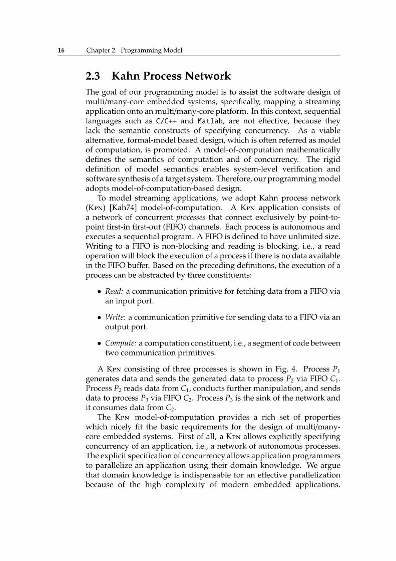
A Kpn consisting of three processes is shown in Fig. 4. Process P1
generates data and sends the generated data to process P2 via FIFO C1.Process P2 reads data from C1, conducts further manipulation, and sendsdata to process P3 via FIFO C2. Process P3 is the sink of the network andit consumes data from C2.
The Kpn model-of-computation provides a rich set of propertieswhich nicely fit the basic requirements for the design of multi/many-core embedded systems. First of all, a Kpn allows explicitly specifyingconcurrency of an application, i.e., a network of autonomous processes.The explicit specification of concurrency allows application programmersto parallelize an application using their domain knowledge. We arguethat domain knowledge is indispensable for an effective parallelizationbecause of the high complexity of modern embedded applications.
2.4. Syntax of Programming Model 17
P1 P2 P3
C1 C2
P1.compute( );
C1.write( );
C1.read( );
P2.compute( );
C2.write( );
C2.read( );
P3.compute( );
Fig. 4: An abstract view of a process network consisting of three processes.
Second, a Kpn separates the communication and computation of anapplication, as the example in Fig. 4 shown. The separation of com-munication and computation allows to separately design communicationand computation of a system. At an early design stage, for instance,application programmers can focus on the design of computation, whilereserving the communication at system level for later refinements. Oneimportant property of Kpn is that a Kpn network is determinate, i.e.,the functional behavior is independent from the timing of processesin the network. The determinism of Kpn decouples the function of anapplication from the underlying architecture of a system, i.e., decouplingwhat a system does and how it does. This property enables separaterefinements of application, architecture, and mapping during the designcycle. We will show in the rest of this thesis how we make use ofthese properties to assist software design of multi/many-core embeddedsystems.
2.4 Syntax of Programming Model
The Kpn model-of-computation defines the semantics of our program-ming model. This section presents the corresponding syntax for thespecification of a multi/many-core embedded system.
2.4.1 Basic Principles
A programming syntax provides a structural description of the variousexpressions that make up legal code in the programming model. Toassist the design of a system, we have identified the following syntacticrequirements.
• Separation of concerns: A key concept of the design of multi/many-core embedded systems is the separation of concerns, i.e., separatingthe application function and the underlying architecture, and

18 Chapter 2. Programming Model
separating the computation and communication of the application.A programming syntax should provide means to establish theseseparations.
• System-level abstraction: Due to the high complexity of modernmulti/many-core embedded systems, describing a system at system-level is an advisable starting point. A system-level abstractionallows verification of a system at an early design stage to detect baddesign decisions as soon as possible. This early decision makingis crucial because of the huge design space of modern embeddedsystems.
• Reuse of legacy code: In modern embedded system design, C/C++are still the dominant development languages to specify embeddedapplications. Whenever a new programming model is designed,the huge amount of legacy code should be considered. Completelyre-writing an application using a new language is time-consumingand error-prone. One would expect to reuse as much legacy code aspossible to reduce the development risk as well as time-to-market.
• Scalability: Future many-core embedded systems exhibit repetitivestructures for both hardware architectures and applications, forinstance, processor arrays and fast Fourier transform, respectively.Sizes and configurations of repetitive components vary for differentdesigns. Therefore, scaling and reconfiguration of repetitivecomponents need to be supported in a systematic way. In addition,the granularity of concurrency for an application should also bereconfigurable in order to explore the design space of a system andto find the optimal candidate design.
In the rest of this section, we present the syntax of our programmingmodel. We separate the specifications of the application, architecture,and mapping of a system. We adopt C/C++/XML as the programminglanguages and define grammar rules for the system specifications. Inaddition, applications written according to this syntax are amenable forautomated refinement with respect to the hardware and the operatingsystem.
2.4.2 Application Specification
We present the syntax for the application specification in this section.The explicit differentiation between computation and communication ofKpn enables the separation between the functionality and structure of anapplication. We use an Xml Schema [MLMK05] to define the syntax for
2.4. Syntax of Programming Model 19
the representation of the structure of the application, i.e., the topologyof the process network. For the functionality of individual processes,we define specific C/C++ coding rules. Using an Xml Schema for thestructure of application allows us, on the one hand, to verify the structureof the process network prior to the final implementation and, on the otherhand, to serve as an interface for other components in a software designtoolchain, for instance, a graphical editor.
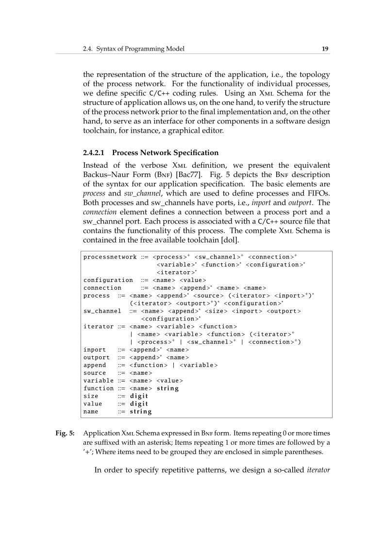
2.4.2.1 Process Network Specification
Instead of the verbose Xml definition, we present the equivalentBackus–Naur Form (Bnf) [Bac77]. Fig. 5 depicts the Bnf descriptionof the syntax for our application specification. The basic elements areprocess and sw_channel, which are used to define processes and FIFOs.Both processes and sw_channels have ports, i.e., inport and outport. Theconnection element defines a connection between a process port and asw_channel port. Each process is associated with a C/C++ source file thatcontains the functionality of this process. The complete Xml Schema iscontained in the free available toolchain [dol].
processnetwork ::= <process>+ <sw_channel >+ <connection >+
<variable >∗ <function >∗ <configuration >∗
<iterator >∗
configuration ::= <name> <value>connection ::= <name> <append>∗ <name> <name>process ::= <name> <append>∗ <source> (<iterator > <inport>+)∗
(<iterator > <outport>+)∗ <configuration >∗
sw_channel ::= <name> <append>∗ <size> <inport> <outport><configuration >∗
iterator ::= <name> <variable > <function >| <name> <variable > <function > (<iterator >+
| <process>+ | <sw_channel >+ | <connection >+)
inport ::= <append>∗ <name>outport ::= <append>∗ <name>append ::= <function > | <variable >source ::= <name>variable ::= <name> <value>function ::= <name> s t r ingsize ::= dig i tvalue ::= dig i tname ::= s t r ing
Fig. 5: Application Xml Schema expressed in Bnf form. Items repeating 0 ormore times
are suffixed with an asterisk; Items repeating 1 or more times are followed by a
’+’; Where items need to be grouped they are enclosed in simple parentheses.
In order to specify repetitive patterns, we design a so-called iterator
20 Chapter 2. Programming Model
<variable value="100" name="N"/>
<process name="P1">
<port type="output" name="10"/>
<source type="c" location="P1.c"/>
</process>
<sw_channel type="fifo" size="10" name="C1">
<iterator name="pipeline" variable="i" range="N">
<process name="P2">
<append function="i"/>
<port type="input" name="1"/>
<port type="output" name="2"/>
<source type="c" location="P2.c"/>
</process>
<sw_channel type="fifo" size="10" name="C2">
<append function="i"/>
<port type="input" name="0"/>
<port type="output" name="1"/>
</sw_channel>
</iterator>
<process name="P3">
<port type="input" name="100"/>
<source type="c" location="P3.c"/>
</process>
...
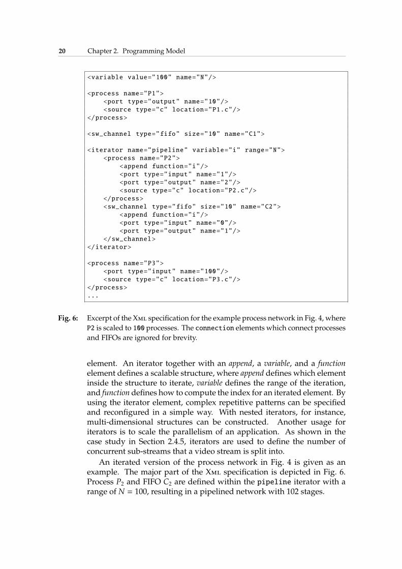
Fig. 6: Excerpt of the Xml specification for the example process network in Fig. 4, where
P2 is scaled to 100 processes. The connection elements which connect processes
and FIFOs are ignored for brevity.
element. An iterator together with an append, a variable, and a functionelement defines a scalable structure, where append defines which elementinside the structure to iterate, variable defines the range of the iteration,and function defines how to compute the index for an iterated element. Byusing the iterator element, complex repetitive patterns can be specifiedand reconfigured in a simple way. With nested iterators, for instance,multi-dimensional structures can be constructed. Another usage foriterators is to scale the parallelism of an application. As shown in thecase study in Section 2.4.5, iterators are used to define the number ofconcurrent sub-streams that a video stream is split into.
An iterated version of the process network in Fig. 4 is given as anexample. The major part of the Xml specification is depicted in Fig. 6.Process P2 and FIFO C2 are defined within the pipeline iterator with arange of N = 100, resulting in a pipelined network with 102 stages.
2.4. Syntax of Programming Model 21
2.4.2.2 Process Specification
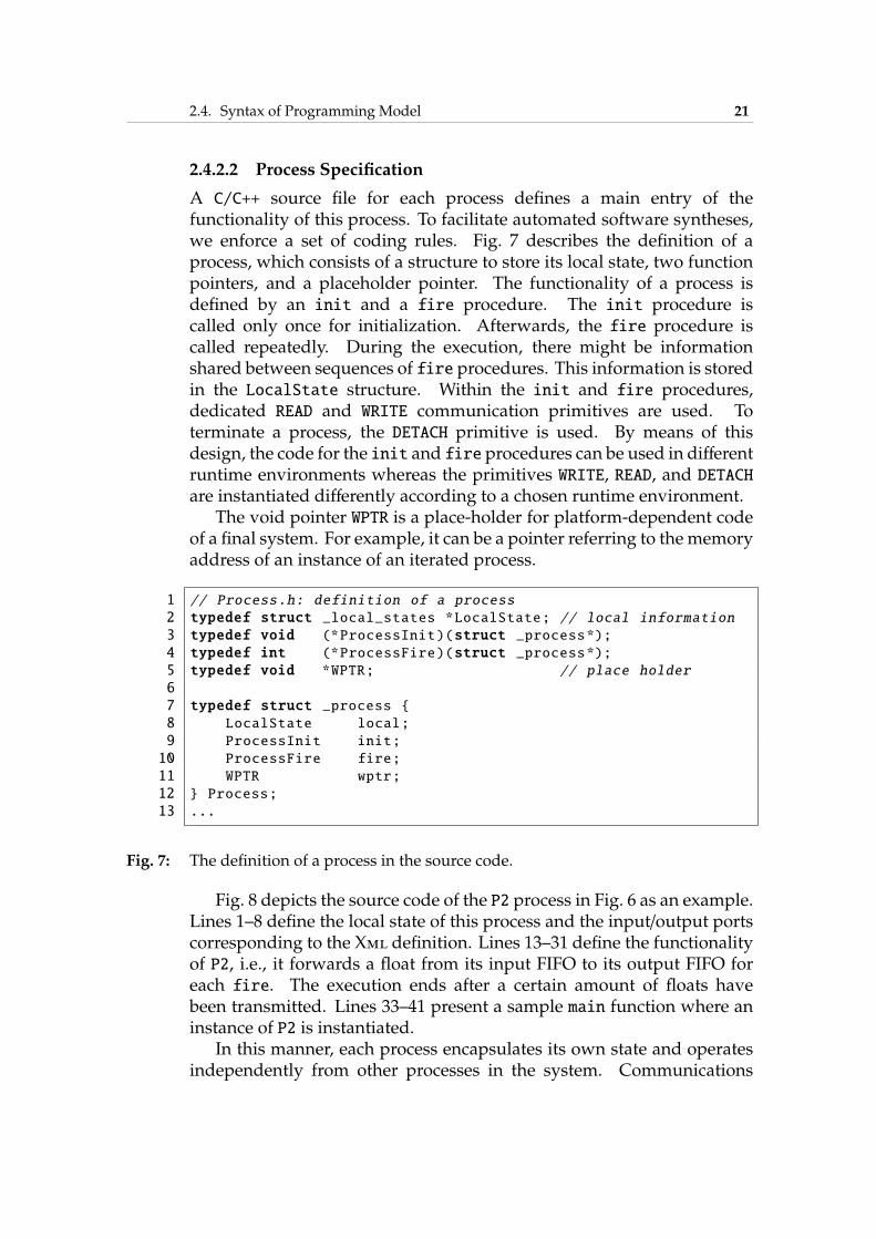
A C/C++ source file for each process defines a main entry of thefunctionality of this process. To facilitate automated software syntheses,we enforce a set of coding rules. Fig. 7 describes the definition of aprocess, which consists of a structure to store its local state, two functionpointers, and a placeholder pointer. The functionality of a process isdefined by an init and a fire procedure. The init procedure iscalled only once for initialization. Afterwards, the fire procedure iscalled repeatedly. During the execution, there might be informationshared between sequences of fire procedures. This information is storedin the LocalState structure. Within the init and fire procedures,dedicated READ and WRITE communication primitives are used. Toterminate a process, the DETACH primitive is used. By means of thisdesign, the code for the init and fire procedures can be used in differentruntime environments whereas the primitives WRITE, READ, and DETACHare instantiated differently according to a chosen runtime environment.
The void pointer WPTR is a place-holder for platform-dependent codeof a final system. For example, it can be a pointer referring to the memoryaddress of an instance of an iterated process.
1 // Process.h: definition of a process
2 typedef struct _local_states *LocalState; // local information
3 typedef void (*ProcessInit)(struct _process*);
4 typedef int (*ProcessFire)(struct _process*);
5 typedef void *WPTR; // place holder
6
7 typedef struct _process {
8 LocalState local;
9 ProcessInit init;
10 ProcessFire fire;
11 WPTR wptr;
12 } Process;
13 ...
Fig. 7: The definition of a process in the source code.
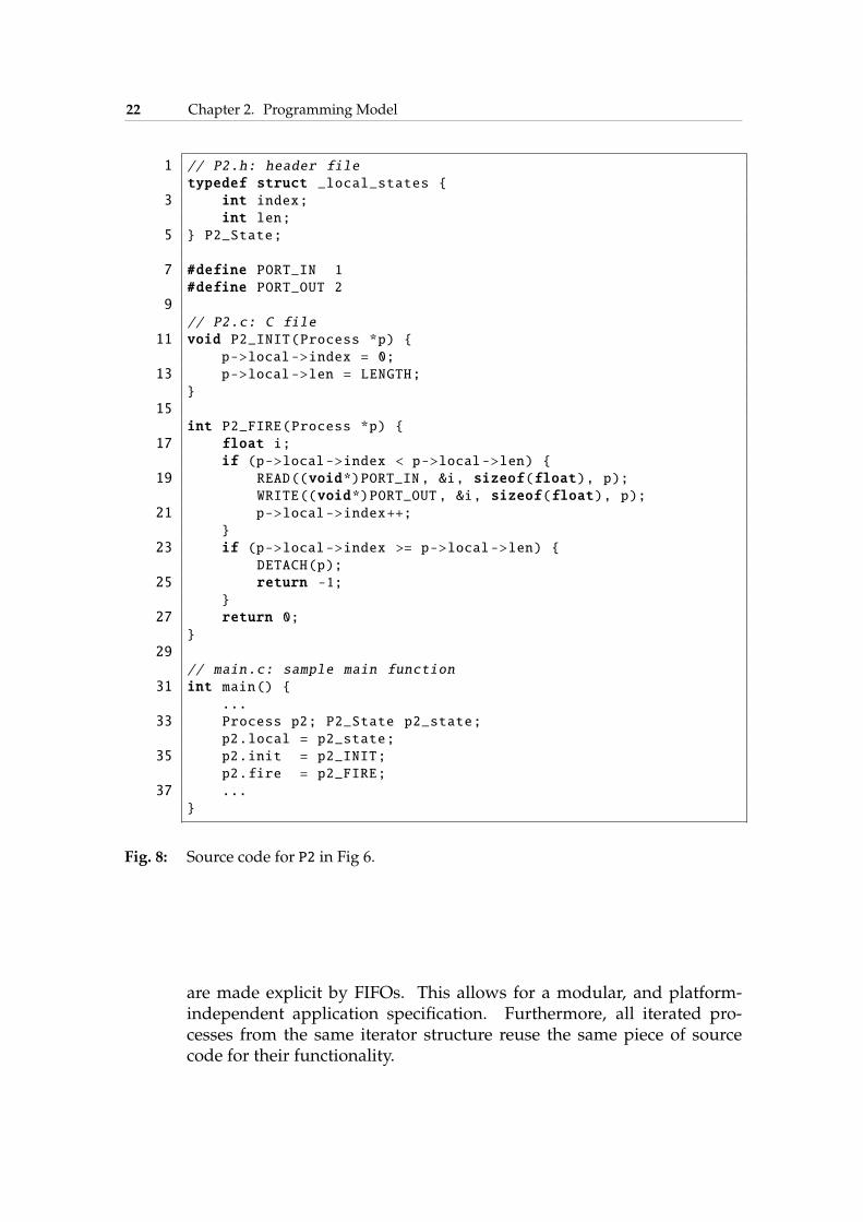
Fig. 8 depicts the source code of the P2 process in Fig. 6 as an example.Lines 1–8 define the local state of this process and the input/output portscorresponding to the Xml definition. Lines 13–31 define the functionalityof P2, i.e., it forwards a float from its input FIFO to its output FIFO foreach fire. The execution ends after a certain amount of floats havebeen transmitted. Lines 33–41 present a sample main function where aninstance of P2 is instantiated.
In this manner, each process encapsulates its own state and operatesindependently from other processes in the system. Communications
22 Chapter 2. Programming Model
1 // P2.h: header file
typedef struct _local_states {
3 int index;
int len;
5 } P2_State;
7 #define PORT_IN 1
#define PORT_OUT 2
9
// P2.c: C file
11 void P2_INIT(Process *p) {
p->local->index = 0;
13 p->local->len = LENGTH;
}
15
int P2_FIRE(Process *p) {
17 float i;
if (p->local->index < p->local->len) {
19 READ((void*)PORT_IN, &i, sizeof(float), p);
WRITE((void*)PORT_OUT , &i, sizeof(float), p);
21 p->local->index++;
}
23 if (p->local->index >= p->local->len) {
DETACH(p);
25 return -1;
}
27 return 0;
}
29
// main.c: sample main function
31 int main() {
...
33 Process p2; P2_State p2_state;
p2.local = p2_state;
35 p2.init = p2_INIT;
p2.fire = p2_FIRE;
37 ...
}
Fig. 8: Source code for P2 in Fig 6.
are made explicit by FIFOs. This allows for a modular, and platform-independent application specification. Furthermore, all iterated pro-cesses from the same iterator structure reuse the same piece of sourcecode for their functionality.
2.4. Syntax of Programming Model 23
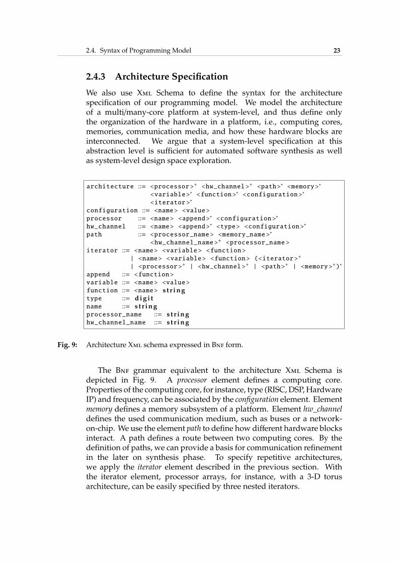
2.4.3 Architecture Specification
We also use Xml Schema to define the syntax for the architecturespecification of our programming model. We model the architectureof a multi/many-core platform at system-level, and thus define onlythe organization of the hardware in a platform, i.e., computing cores,memories, communication media, and how these hardware blocks areinterconnected. We argue that a system-level specification at thisabstraction level is sufficient for automated software synthesis as wellas system-level design space exploration.
architecture ::= <processor >+ <hw_channel >+ <path>∗ <memory>∗
<variable >∗ <function >∗ <configuration >∗
<iterator >∗
configuration ::= <name> <value>processor ::= <name> <append>∗ <configuration >∗
hw_channel ::= <name> <append>∗ <type> <configuration >∗
path ::= <processor_name > <memory_name >∗
<hw_channel_name >+ <processor_name >
iterator ::= <name> <variable > <function >| <name> <variable > <function > (<iterator >+
| <processor >+ | <hw_channel >+ | <path>+ | <memory>+)∗
append ::= <function >variable ::= <name> <value>function ::= <name> s t r ingtype ::= dig i tname ::= s t r ingprocessor_name ::= s t r inghw_channel_name ::= s t r ing
Fig. 9: Architecture Xml schema expressed in Bnf form.
The Bnf grammar equivalent to the architecture Xml Schema isdepicted in Fig. 9. A processor element defines a computing core.Properties of the computing core, for instance, type (RISC, DSP,HardwareIP) and frequency, can be associated by the configuration element. Elementmemory defines a memory subsystem of a platform. Element hw_channeldefines the used communication medium, such as buses or a network-on-chip. We use the element path to define how different hardware blocksinteract. A path defines a route between two computing cores. By thedefinition of paths, we can provide a basis for communication refinementin the later on synthesis phase. To specify repetitive architectures,we apply the iterator element described in the previous section. Withthe iterator element, processor arrays, for instance, with a 3-D torusarchitecture, can be easily specified by three nested iterators.
24 Chapter 2. Programming Model
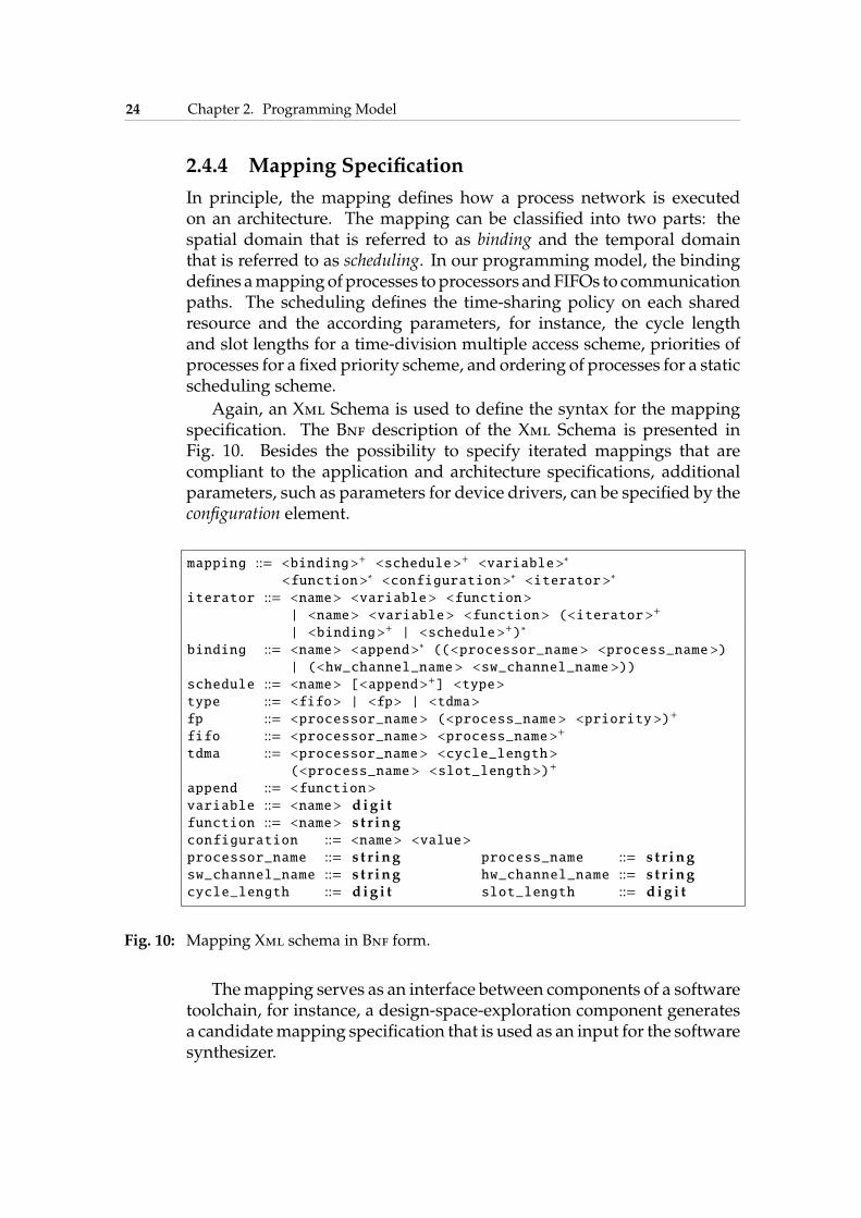
2.4.4 Mapping Specification
In principle, the mapping defines how a process network is executedon an architecture. The mapping can be classified into two parts: thespatial domain that is referred to as binding and the temporal domainthat is referred to as scheduling. In our programming model, the bindingdefines amappingofprocesses toprocessors andFIFOs to communicationpaths. The scheduling defines the time-sharing policy on each sharedresource and the according parameters, for instance, the cycle lengthand slot lengths for a time-division multiple access scheme, priorities ofprocesses for a fixed priority scheme, and ordering of processes for a staticscheduling scheme.
Again, an Xml Schema is used to define the syntax for the mappingspecification. The Bnf description of the Xml Schema is presented inFig. 10. Besides the possibility to specify iterated mappings that arecompliant to the application and architecture specifications, additionalparameters, such as parameters for device drivers, can be specified by theconfiguration element.
mapping ::= <binding>+ <schedule >+ <variable >∗
<function >∗ <configuration >∗ <iterator >∗
iterator ::= <name> <variable > <function >| <name> <variable > <function > (<iterator >+
| <binding>+ | <schedule >+)∗
binding ::= <name> <append>∗ ((<processor_name > <process_name >)| (<hw_channel_name > <sw_channel_name >))
schedule ::= <name> [<append>+] <type>type ::= <fifo> | <fp> | <tdma>fp ::= <processor_name > (<process_name > <priority >)+
fifo ::= <processor_name > <process_name >+
tdma ::= <processor_name > <cycle_length >(<process_name > <slot_length >)+
append ::= <function >variable ::= <name> dig i tfunction ::= <name> s t r ingconfiguration ::= <name> <value>processor_name ::= s t r ing process_name ::= s t r ingsw_channel_name ::= s t r ing hw_channel_name ::= s t r ingcycle_length ::= dig i t slot_length ::= dig i t
Fig. 10: Mapping Xml schema in Bnf form.
Themapping serves as an interface between components of a softwaretoolchain, for instance, a design-space-exploration component generatesa candidatemapping specification that is used as an input for the softwaresynthesizer.
2.4. Syntax of Programming Model 25
2.4.5 Experimental Results
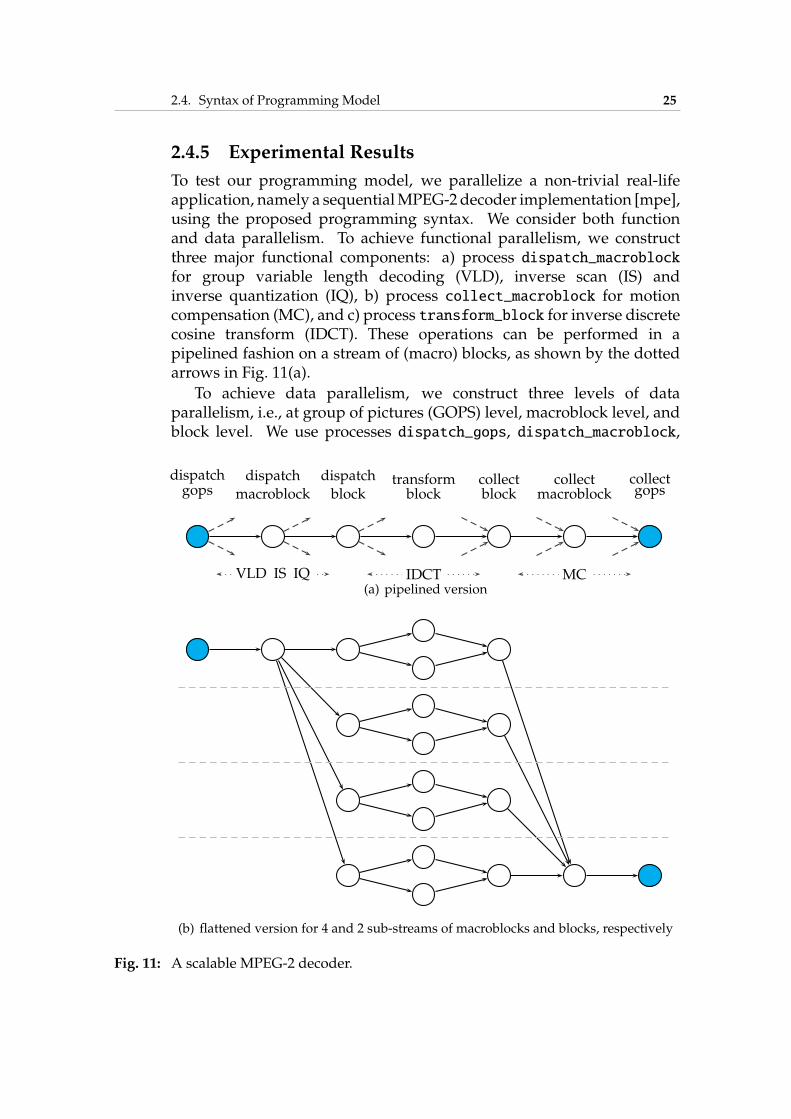
To test our programming model, we parallelize a non-trivial real-lifeapplication, namely a sequentialMPEG-2 decoder implementation [mpe],using the proposed programming syntax. We consider both functionand data parallelism. To achieve functional parallelism, we constructthree major functional components: a) process dispatch_macroblockfor group variable length decoding (VLD), inverse scan (IS) andinverse quantization (IQ), b) process collect_macroblock for motioncompensation (MC), and c) process transform_block for inverse discretecosine transform (IDCT). These operations can be performed in apipelined fashion on a stream of (macro) blocks, as shown by the dottedarrows in Fig. 11(a).
To achieve data parallelism, we construct three levels of dataparallelism, i.e., at group of pictures (GOPS) level, macroblock level, andblock level. We use processes dispatch_gops, dispatch_macroblock,
dispatchgops
dispatch
macroblock
dispatch
blocktransformblock
collectblock
collectmacroblock
collectgops
VLD IS IQ IDCT MC(a) pipelined version
(b) flattened version for 4 and 2 sub-streams of macroblocks and blocks, respectively
Fig. 11: A scalable MPEG-2 decoder.
26 Chapter 2. Programming Model
and dispatch_block to split a stream of GOPS, macroblocks, and blocksinto multiple independent sub-streams, respectively. Correspondingly,processes collect_block, collect_macroblock, and collect_gops areused to collect the decoded data and reassemble them into streams in thecorrect order. The data parallelism is indicated by the solid arrows inFig. 11(a).
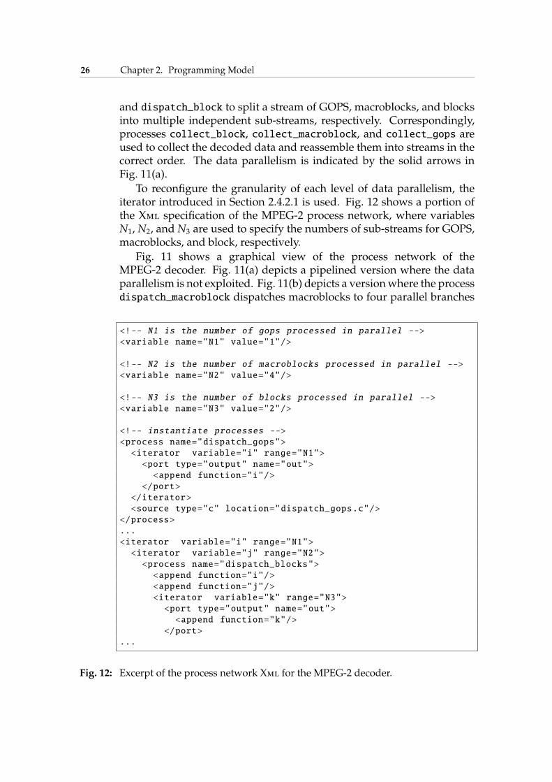
To reconfigure the granularity of each level of data parallelism, theiterator introduced in Section 2.4.2.1 is used. Fig. 12 shows a portion ofthe Xml specification of the MPEG-2 process network, where variablesN1, N2, and N3 are used to specify the numbers of sub-streams for GOPS,macroblocks, and block, respectively.
Fig. 11 shows a graphical view of the process network of theMPEG-2 decoder. Fig. 11(a) depicts a pipelined version where the dataparallelism is not exploited. Fig. 11(b) depicts a versionwhere the processdispatch_macroblock dispatches macroblocks to four parallel branches
<!-- N1 is the number of gops processed in parallel -->
<variable name="N1" value="1"/>
<!-- N2 is the number of macroblocks processed in parallel -->
<variable name="N2" value="4"/>
<!-- N3 is the number of blocks processed in parallel -->
<variable name="N3" value="2"/>
<!-- instantiate processes -->
<process name="dispatch_gops">
<iterator variable="i" range="N1">
<port type="output" name="out">
<append function="i"/>
</port>
</iterator>
<source type="c" location="dispatch_gops.c"/>
</process>
...
<iterator variable="i" range="N1">
<iterator variable="j" range="N2">
<process name="dispatch_blocks">
<append function="i"/>
<append function="j"/>
<iterator variable="k" range="N3">
<port type="output" name="out">
<append function="k"/>
</port>
...
Fig. 12: Excerpt of the process network Xml for the MPEG-2 decoder.
2.5. Windowed-FIFO Communication 27
and each branch will again be dispatched by dispatch_block to two sub-branches transform_block, resulting in a network of 20 processes. Notethat the source code of these two versions is identical. The only differenceis the values of variables N1, N2, and N3 in the Xml specification.
We also report the code size in terms of lines-of-code. The referencesequential implementation [mpe] contains 5727 lines of C code. Theparallel version using our programming model contains 4004 lines ofC code and 319 lines of Xml code. The difference can be explained bythe fact that the reference code is a full-fledged compilable source codefor IA-32 architecture whereas our version only contains the platform-independent portion of the decoder.
From this experiment, we conclude that our programming model ispracticable. In the next two sections, we will discuss the efficiency of ourprogramming model in terms of syntactic variation of the Kpn model-of-computation as well as runtime environments.
2.5 Windowed-FIFO Communication
The Kpn model-of-computation provides a set of useful properties fordesigning multi/many-core embedded systems. Partly, these propertiesare based on the FIFO communication. The rigorous FIFO commu-nication, however, has limitations in terms of programmability andefficiency. In this section, we present a syntactic variation for the FIFOcommunication of Kpn to increase the efficiency and programmability ofFIFO communication.
2.5.1 Motivation
Although the Kpn model-of-computation offers a simple interface forprogramming, it also has limitations that make the implementationof streaming applications difficult or inefficient. Furthermore, thecommunication overhead might overshadow the performance gainedby the coarse-grain parallelism. A few syntactic limitations that are ofinterest are addressed in the following:
• Reordering: A Kpn FIFO behaves in a strict first-in first-out manner,which does not allow reading data in an order other than the one inwhich the data have been written.
• Non-destructive read: A Kpn FIFO does not allow reading the samedata itemmore than once. After a data item is read, it will be deletedfrom the FIFO memory.
28 Chapter 2. Programming Model
• Skipping: It is not possible to remove adata item fromaFIFOwithouta read operation. Even if the FIFO contains unwanted data, allthese unwanted data have to be read out before subsequent datacan be accessed. An example for a skipping scenario is described inSection 2.5.5.2.
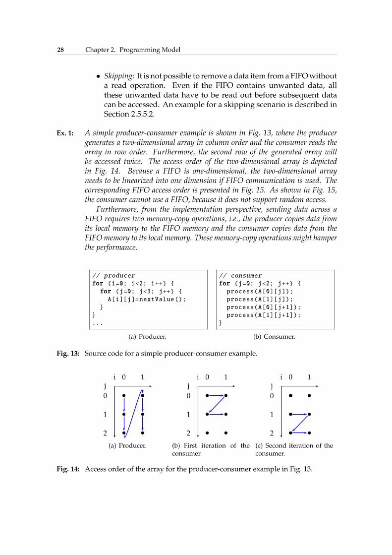
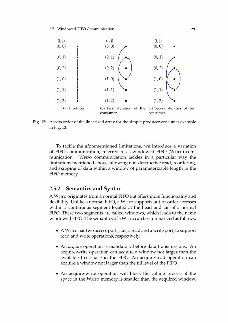
Ex. 1: A simple producer-consumer example is shown in Fig. 13, where the producergenerates a two-dimensional array in column order and the consumer reads thearray in row order. Furthermore, the second row of the generated array willbe accessed twice. The access order of the two-dimensional array is depictedin Fig. 14. Because a FIFO is one-dimensional, the two-dimensional arrayneeds to be linearized into one dimension if FIFO communication is used. Thecorresponding FIFO access order is presented in Fig. 15. As shown in Fig. 15,the consumer cannot use a FIFO, because it does not support random access.
Furthermore, from the implementation perspective, sending data across aFIFO requires two memory-copy operations, i.e., the producer copies data fromits local memory to the FIFO memory and the consumer copies data from theFIFOmemory to its local memory. These memory-copy operations might hamperthe performance.
// producer
for (i=0; i<2; i++) {
for (j=0; j<3; j++) {
A[i][j]=nextValue();
}
}
...
(a) Producer.
// consumer
for (j=0; j<2; j++) {
process(A[0][j]);
process(A[1][j]);
process(A[0][j+1]);
process(A[1][j+1]);
}
(b) Consumer.
Fig. 13: Source code for a simple producer-consumer example.
ij
0 1
0
1
2
(a) Producer.
ij
0 1
0
1
2
(b) First iteration of theconsumer.
ij
0 1
0
1
2
(c) Second iteration of theconsumer.
Fig. 14: Access order of the array for the producer-consumer example in Fig. 13.
2.5. Windowed-FIFO Communication 29
(i, j)
(0, 0)
(0, 1)
(0, 2)
(1, 0)
(1, 1)
(1, 2)
(a) Producer.
(i, j)
(0, 0)
(0, 1)
(0, 2)
(1, 0)
(1, 1)
(1, 2)
(b) First iteration of theconsumer.
(i, j)
(0, 0)
(0, 1)
(0, 2)
(1, 0)
(1, 1)
(1, 2)
(c) Second iteration of theconsumer.
Fig. 15: Access order of the linearized array for the simple producer-consumer example
in Fig. 13.
To tackle the aforementioned limitations, we introduce a variationof FIFO communication, referred to as windowed FIFO (Wfifo) com-munication. Wfifo communication tackles in a particular way thelimitations mentioned above, allowing non-destructive read, reordering,and skipping of data within a window of parameterizable length in theFIFO memory.
2.5.2 Semantics and Syntax
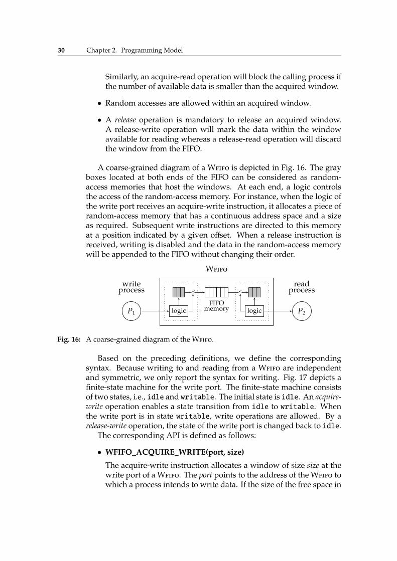
AWfifo originates from a normal FIFO but offers more functionality andflexibility. Unlike a normal FIFO, a Wfifo supports out-of-order accesseswithin a continuous segment located at the head and tail of a normalFIFO. These two segments are called windows, which leads to the namewindowed FIFO. The semantics of aWfifo can be summarized as follows:
• AWfifo has two access ports, i.e., a read and awrite port, to supportread and write operations, respectively.
• An acquire operation is mandatory before data transmissions. Anacquire-write operation can acquire a window not larger than theavailable free space in the FIFO. An acquire-read operation canacquire a window not larger than the fill level of the FIFO.
• An acquire-write operation will block the calling process if thespace in the Wfifo memory is smaller than the acquired window.
30 Chapter 2. Programming Model
Similarly, an acquire-read operation will block the calling process ifthe number of available data is smaller than the acquired window.
• Random accesses are allowed within an acquired window.
• A release operation is mandatory to release an acquired window.A release-write operation will mark the data within the windowavailable for reading whereas a release-read operation will discardthe window from the FIFO.
A coarse-grained diagram of a Wfifo is depicted in Fig. 16. The grayboxes located at both ends of the FIFO can be considered as random-access memories that host the windows. At each end, a logic controlsthe access of the random-access memory. For instance, when the logic ofthe write port receives an acquire-write instruction, it allocates a piece ofrandom-access memory that has a continuous address space and a sizeas required. Subsequent write instructions are directed to this memoryat a position indicated by a given offset. When a release instruction isreceived, writing is disabled and the data in the random-access memorywill be appended to the FIFO without changing their order.
logic logicP1 P2
writeprocess
readprocess
Wfifo
FIFOmemory
Fig. 16: A coarse-grained diagram of the Wfifo.
Based on the preceding definitions, we define the correspondingsyntax. Because writing to and reading from a Wfifo are independentand symmetric, we only report the syntax for writing. Fig. 17 depicts afinite-state machine for the write port. The finite-state machine consistsof two states, i.e., idle and writable. The initial state is idle. An acquire-write operation enables a state transition from idle to writable. Whenthe write port is in state writable, write operations are allowed. By arelease-write operation, the state of the write port is changed back to idle.
The corresponding API is defined as follows:
• WFIFO_ACQUIRE_WRITE(port, size)
The acquire-write instruction allocates a window of size size at thewrite port of a Wfifo. The port points to the address of the Wfifo towhich a process intends to write data. If the size of the free space in

2.5. Windowed-FIFO Communication 31
idle writable
acquire-write
release-write
write
Fig. 17: The finite-state machine for the write port of a Wfifo.
theWfifo is smaller than size, then this instruction blocks the callingprocess until enough memory is available.
• WFIFO_WRITE(port, offset, data)
The write instruction writes the data to the write window at theposition indicated by the offset. This instruction can be repeated anunlimited number of times. It is possible to write the same offsetposition more than once. In the case of multiple writing to a sameoffset address, the new value will overwrite the old one. If an offsetposition is never written, its value is undefined.
• WFIFO_RELEASE_WRITE(port)
The release instruction terminates the writing phase and appendsthe content of the window to an internal FIFO, from which it canlater be read. After releasing, no further writing to the window ispossible. Before more data can be written to the Wfifo, a new writewindow must be acquired.
The finite-state machine and API for the read port are analogous tothe write port. They contain acquire-read, read, and release-read operations.An acquire-read operation succeeds if there are enough data in a Wfifomemory for the acquired read window. After successful acquisition, datacan be read from thewindow. The release instruction deletes the acquiredwindow from the Wfifo.
2.5.3 Properties
A process network using Wfifo communication has properties similarto a Kpn. In particular, we will show that a Wfifo process network isdeterminate, i.e., the functional behavior is independent on the timing ofthe processes in the process network.
Lem. 1: A Wfifo process network can be simulated by a process network with bothblocking-read and blocking-write semantics.
Proof. The fundamental difference between a Wfifo process networkand a process network with blocking semantics is the replacement of
32 Chapter 2. Programming Model
FIFO communication with Wfifo. It must be shown that the windowedsemantics can be implemented using a FIFO with blocking semantics.Given the property that the read and write windows do not overlap eachother, the segment between the read and write windows is strictly first-come first-out, i.e., equivalent to a FIFO. The window mechanism canbe transformed into a software implementation within the connectedprocesses. For writing a Wfifo, when an acquire-write operation isinvoked, a segment in the local memory with a size as the size of theacquiredwindow is allocated. Subsequentwrite operations are redirectedto this segment until a release-write operation is received. The release-write operation will move the data within this segment to the FIFOmemory. Reading a Wfifo is similar. When an acquire-read operationis invoked, a segment in the local memory with a size as the size ofthe acquired window is allocated and data in the acquired window aremoved from the FIFO memory to this segment. All subsequent readoperations are redirected to this segment, i.e. reading from this piece oflocal memory. This segment will be freed upon a release-read operation.Under this transformation, a Wfifo process network can be simulated bya process network with blocking-read and blocking-write semantics.
�
Lem. 2: A process network with blocking-write (and blocking-read) semantics can besimulated by a KPN.
Lem. 2 is a known result [GB03]. Nevertheless, we show in thefollowing an intuitive description for how to simulate a process networkwith blocking semantics using a Kpn. A blocking-write semantics of aFIFO implies a bounded FIFO, i.e., with a finite size. A bounded FIFO,say Fi, with a size s in a process network can be replaced by a pair ofunbounded FIFOswith size s, where one (forward) has the same directionas Fi and the other (backward) has the opposite direction. If Fi initiallydoes not contain any data, i.e., an empty state, the backward FIFO is setto contain s dummy data tokens. In the source code of the calling process,a write operation to Fi is transformed into two operations: first read adummy token from the backward FIFO, and then write the actual data tothe forward FIFO. Similarly, a read operation of Fi is transformed into twooperations as well: first write a dummy token to the backward FIFO, andthen read the actual data from the forward FIFO. This backward-pressuremechanism guarantees that there are never more than s data tokens in theforward FIFO, which is tantamount to a bounded FIFOwith size s. Underthis transformation, a bounded FIFO can be implemented with a pair ofunbounded FIFOs with non-blocking write and blocking-read semantics.Therefore, the lemma holds.
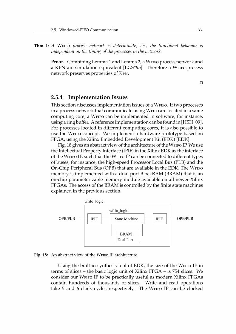
2.5. Windowed-FIFO Communication 33
Thm. 1: A Wfifo process network is determinate, i.e., the functional behavior isindependent on the timing of the processes in the network.
Proof. Combining Lemma 1 and Lemma 2, aWfifo process network anda KPN are simulation equivalent [LGS+95]. Therefore a Wfifo processnetwork preserves properties of Kpn.
�
2.5.4 Implementation Issues
This section discusses implementation issues of aWfifo. If two processesin a process network that communicate usingWfifo are located in a samecomputing core, a Wfifo can be implemented in software, for instance,using a ringbuffer. A reference implementation canbe found in [HSH+09].For processes located in different computing cores, it is also possible touse the Wfifo concept. We implement a hardware prototype based onFPGA, using the Xilinx Embedded Development Kit (EDK) [EDK].
Fig. 18 gives an abstract viewof the architecture of theWfifo IP.Weusethe Intellectual Property Interface (IPIF) in the Xilinx EDK as the interfaceof theWfifo IP, such that theWfifo IP can be connected to different typesof buses, for instance, the high-speed Processor Local Bus (PLB) and theOn-Chip Peripheral Bus (OPB) that are available in the EDK. The Wfifomemory is implemented with a dual-port BlockRAM (BRAM) that is anon-chip parameterizable memory module available on all newer XilinxFPGAs. The access of the BRAM is controlled by the finite state machinesexplained in the previous section.
wfifo_logic
BRAM
Dual Port
IPIFIPIF
wfifo_logic
OPB/PLBOPB/PLB State Machine
Fig. 18: An abstract view of the Wfifo IP architecture.
Using the built-in synthesis tool of EDK, the size of the Wfifo IP interms of slices – the basic logic unit of Xilinx FPGA – is 754 slices. Weconsider our Wfifo IP to be practically useful as modern Xilinx FPGAscontain hundreds of thousands of slices. Write and read operationstake 5 and 6 clock cycles respectively. The Wfifo IP can be clocked
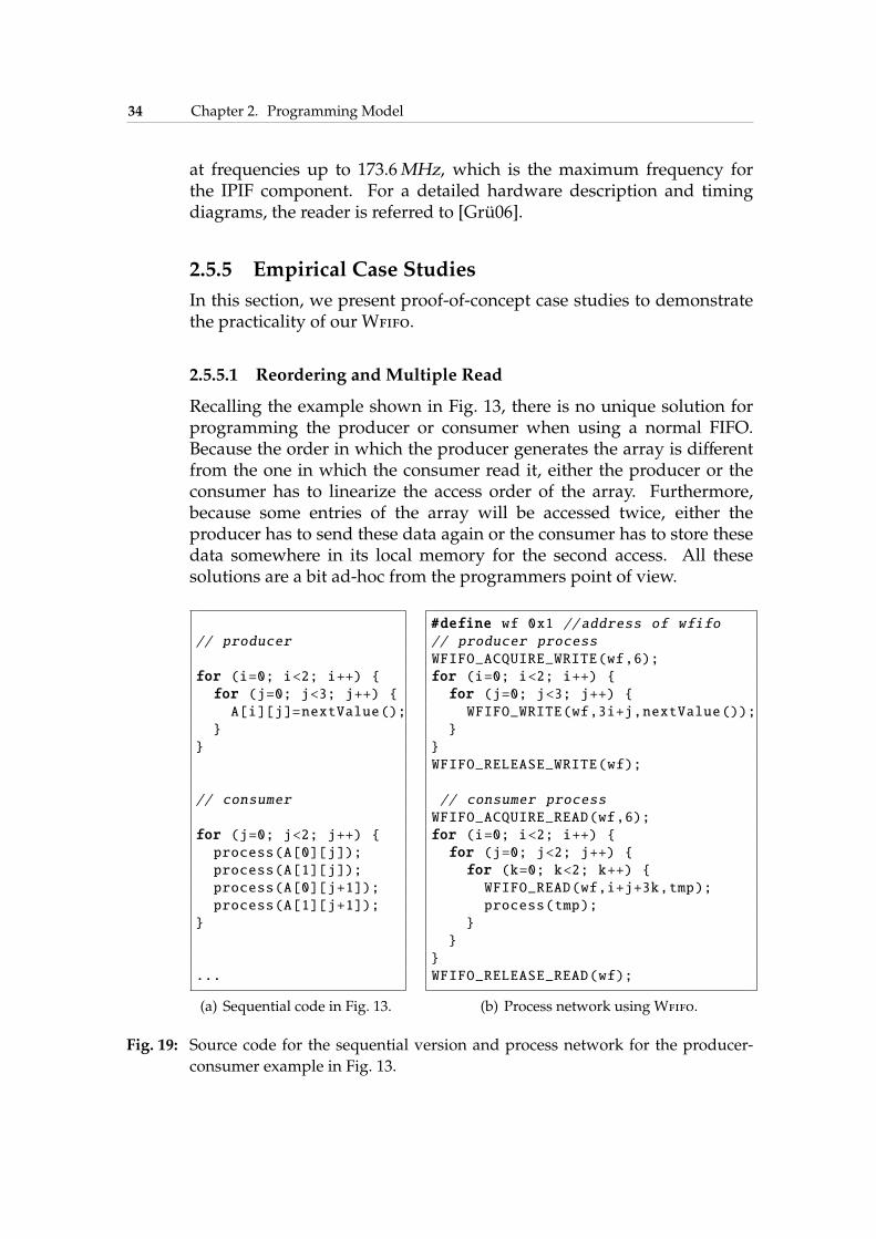
34 Chapter 2. Programming Model
at frequencies up to 173.6MHz, which is the maximum frequency forthe IPIF component. For a detailed hardware description and timingdiagrams, the reader is referred to [Grü06].
2.5.5 Empirical Case Studies
In this section, we present proof-of-concept case studies to demonstratethe practicality of our Wfifo.
2.5.5.1 Reordering and Multiple Read
Recalling the example shown in Fig. 13, there is no unique solution forprogramming the producer or consumer when using a normal FIFO.Because the order in which the producer generates the array is differentfrom the one in which the consumer read it, either the producer or theconsumer has to linearize the access order of the array. Furthermore,because some entries of the array will be accessed twice, either theproducer has to send these data again or the consumer has to store thesedata somewhere in its local memory for the second access. All thesesolutions are a bit ad-hoc from the programmers point of view.
// producer
for (i=0; i<2; i++) {
for (j=0; j<3; j++) {
A[i][j]=nextValue();
}
}
// consumer
for (j=0; j<2; j++) {
process(A[0][j]);
process(A[1][j]);
process(A[0][j+1]);
process(A[1][j+1]);
}
...
(a) Sequential code in Fig. 13.
#define wf 0x1 //address of wfifo
// producer process
WFIFO_ACQUIRE_WRITE(wf,6);
for (i=0; i<2; i++) {
for (j=0; j<3; j++) {
WFIFO_WRITE(wf,3i+j,nextValue());
}
}
WFIFO_RELEASE_WRITE(wf);
// consumer process
WFIFO_ACQUIRE_READ(wf,6);
for (i=0; i<2; i++) {
for (j=0; j<2; j++) {
for (k=0; k<2; k++) {
WFIFO_READ(wf,i+j+3k,tmp);
process(tmp);
}
}
}
WFIFO_RELEASE_READ(wf);
(b) Process network using Wfifo.
Fig. 19: Source code for the sequential version and process network for the producer-
consumer example in Fig. 13.
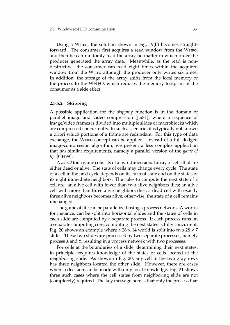
2.5. Windowed-FIFO Communication 35
Using a Wfifo, the solution shown in Fig. 19(b) becomes straight-forward. The consumer first acquires a read window from the Wfifo,and then he can randomly read the array no matter in which order theproducer generated the array data. Meanwhile, as the read is non-destructive, the consumer can read eight times within the acquiredwindow from the Wfifo although the producer only writes six times.In addition, the storage of the array shifts from the local memory ofthe process to the WFIFO, which reduces the memory footprint of theconsumer as a side effect.
2.5.5.2 Skipping
A possible application for the skipping function is in the domain ofparallel image and video compression [Jai81], where a sequence ofimage/video frames is divided into multiple slides or macroblocks whichare compressed concurrently. In such a scenario, it is typically not knowna priori which portions of a frame are redundant. For this type of dataexchange, the Wfifo concept can be applied. Instead of a full-fledgedimage-compression algorithm, we present a less complex applicationthat has similar requirements, namely a parallel version of the game oflife [GH99].
Aworld for a game consists of a two-dimensional array of cells that areeither dead or alive. The stats of cells may change every cycle. The stateof a cell in the next cycle depends on its current state and on the states ofits eight immediate neighbors. The rules to compute the next state of acell are: an alive cell with fewer than two alive neighbors dies; an alivecell with more than three alive neighbors dies; a dead cell with exactlythree alive neighbors becomes alive; otherwise, the state of a cell remainsunchanged.
The game of life can be parallelized using a process network. Aworld,for instance, can be split into horizontal slides and the states of cells ineach slide are computed by a separate process. If each process runs ona separate computing core, computing the next states is fully concurrent.Fig. 20 shows an example where a 28 × 14 world is split into two 28 × 7slides. These two slides are processed by two separate processes, namelyprocess X and Y, resulting in a process network with two processes.
For cells at the boundaries of a slide, determining their next states,in principle, requires knowledge of the states of cells located at theneighboring slide. As shown in Fig. 20, any cell in the two gray rowshas three neighbors located the other slide. However, there are caseswhere a decision can be made with only local knowledge. Fig. 21 showsthree such cases where the cell states from neighboring slide are not(completely) required. The key message here is that only the process that
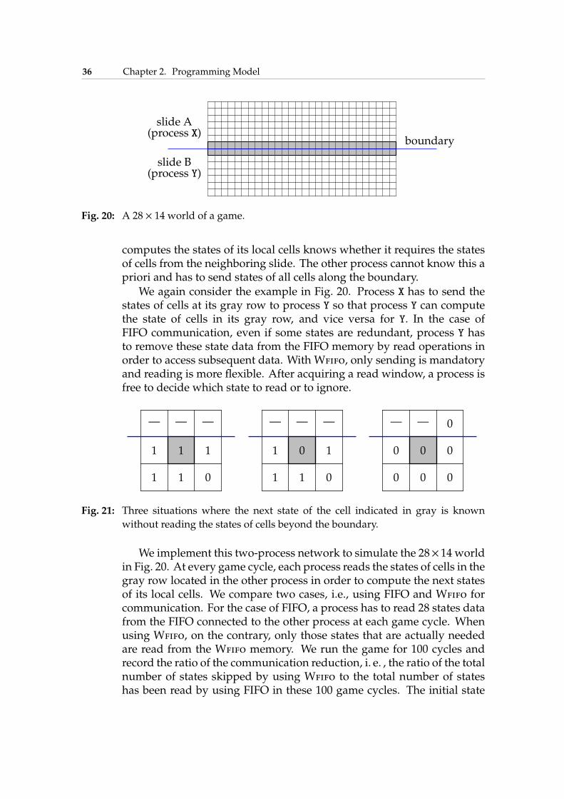
36 Chapter 2. Programming Model
boundary
slide A(process X)
slide B(process Y)
Fig. 20: A 28 × 14 world of a game.
computes the states of its local cells knows whether it requires the statesof cells from the neighboring slide. The other process cannot know this apriori and has to send states of all cells along the boundary.
We again consider the example in Fig. 20. Process X has to send thestates of cells at its gray row to process Y so that process Y can computethe state of cells in its gray row, and vice versa for Y. In the case ofFIFO communication, even if some states are redundant, process Y hasto remove these state data from the FIFO memory by read operations inorder to access subsequent data. With Wfifo, only sending is mandatoryand reading is more flexible. After acquiring a read window, a process isfree to decide which state to read or to ignore.
1 1 0
1 1 1
— — —
1 1 0
1 0 1
— — —
0 0 0
0 0 0
— — 0
Fig. 21: Three situations where the next state of the cell indicated in gray is known
without reading the states of cells beyond the boundary.
We implement this two-process network to simulate the 28× 14 worldin Fig. 20. At every game cycle, each process reads the states of cells in thegray row located in the other process in order to compute the next statesof its local cells. We compare two cases, i.e., using FIFO and Wfifo forcommunication. For the case of FIFO, a process has to read 28 states datafrom the FIFO connected to the other process at each game cycle. Whenusing Wfifo, on the contrary, only those states that are actually neededare read from the Wfifo memory. We run the game for 100 cycles andrecord the ratio of the communication reduction, i. e. , the ratio of the totalnumber of states skipped by using Wfifo to the total number of stateshas been read by using FIFO in these 100 game cycles. The initial state
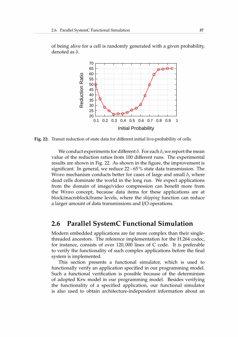
2.6. Parallel SystemC Functional Simulation 37
of being alive for a cell is randomly generated with a given probability,denoted as δ.
20 25 30 35 40 45 50 55 60 65 70
0.1 0.2 0.3 0.4 0.5 0.6 0.7 0.8 0.9 1
Red
uctio
n R
atio
Initial Probability
Fig. 22: Transit reduction of state data for different initial live-probability of cells.
Weconduct experiments for different δ. For each δ, we report themeanvalue of the reduction ratios from 100 different runs. The experimentalresults are shown in Fig. 22. As shown in the figure, the improvement issignificant. In general, we reduce 22 – 65% state data transmission. TheWfifo mechanism conducts better for cases of large and small δ, wheredead cells dominate the world in the long run. We expect applicationsfrom the domain of image/video compression can benefit more fromthe Wfifo concept, because data items for these applications are atblock/macroblock/frame levels, where the skipping function can reducea larger amount of data transmissions and I/O operations.
2.6 Parallel SystemC Functional Simulation
Modern embedded applications are far more complex than their single-threaded ancestors. The reference implementation for the H.264 codec,for instance, consists of over 120, 000 lines of C code. It is preferableto verify the functionality of such complex applications before the finalsystem is implemented.
This section presents a functional simulator, which is used tofunctionally verify an application specified in our programming model.Such a functional verification is possible because of the determinismof adopted Kpn model in our programming model. Besides verifyingthe functionality of a specified application, our functional simulatoris also used to obtain architecture-independent information about an
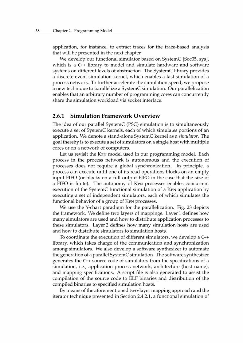
38 Chapter 2. Programming Model
application, for instance, to extract traces for the trace-based analysisthat will be presented in the next chapter.
We develop our functional simulator based on SystemC [Soc05, sys],which is a C++ library to model and simulate hardware and softwaresystems on different levels of abstraction. The SystemC library providesa discrete-event simulation kernel, which enables a fast simulation of aprocess network. To further accelerate the simulation speed, we proposea new technique to parallelize a SystemC simulation. Our parallelizationenables that an arbitrary number of programming cores can concurrentlyshare the simulation workload via socket interface.
2.6.1 Simulation Framework Overview
The idea of our parallel SystemC (PSC) simulation is to simultaneouslyexecute a set of SystemC kernels, each of which simulates portions of anapplication. We denote a stand-alone SystemC kernel as a simulator. Thegoal thereby is to execute a set of simulators on a single host withmultiplecores or on a network of computers.
Let us revisit the Kpn model used in our programming model. Eachprocess in the process network is autonomous and the execution ofprocesses does not require a global synchronization. In principle, aprocess can execute until one of its read operations blocks on an emptyinput FIFO (or blocks on a full output FIFO in the case that the size ofa FIFO is finite). The autonomy of Kpn processes enables concurrentexecution of the SystemC functional simulation of a Kpn application byexecuting a set of independent simulators, each of which simulates thefunctional behavior of a group of Kpn processes.
We use the Y-chart paradigm for the parallelization. Fig. 23 depictsthe framework. We define two layers of mappings. Layer 1 defines howmany simulators are used and how to distribute application processes tothese simulators. Layer 2 defines how many simulation hosts are usedand how to distribute simulators to simulation hosts.
To coordinate the execution of different simulators, we develop a C++library, which takes charge of the communication and synchronizationamong simulators. We also develop a software synthesizer to automatethe generation of a parallel SystemC simulation. The software synthesizergenerates the C++ source code of simulators from the specifications of asimulation, i.e., application process network, architecture (host name),and mapping specifications. A script file is also generated to assist thecompilation of the source code to ELF binaries and distribution of thecompiled binaries to specified simulation hosts.
Bymeans of the aforementioned two-layermapping approach and theiterator technique presented in Section 2.4.2.1, a functional simulation of
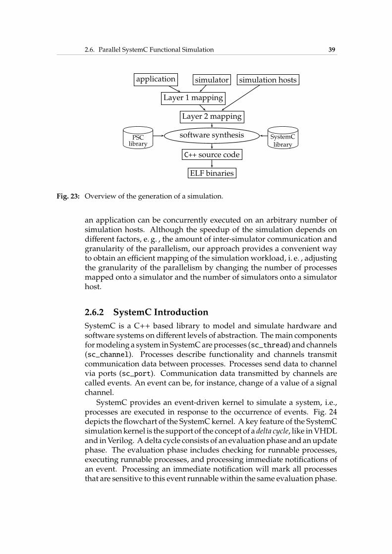
2.6. Parallel SystemC Functional Simulation 39
PSClibrary
SystemClibrary
application simulator simulation hosts
Layer 1 mapping
Layer 2 mapping
software synthesis
C++ source code
ELF binaries
Fig. 23: Overview of the generation of a simulation.
an application can be concurrently executed on an arbitrary number ofsimulation hosts. Although the speedup of the simulation depends ondifferent factors, e. g. , the amount of inter-simulator communication andgranularity of the parallelism, our approach provides a convenient wayto obtain an efficient mapping of the simulation workload, i. e. , adjustingthe granularity of the parallelism by changing the number of processesmapped onto a simulator and the number of simulators onto a simulatorhost.
2.6.2 SystemC Introduction
SystemC is a C++ based library to model and simulate hardware andsoftware systems on different levels of abstraction. Themain componentsformodeling a system in SystemCareprocesses (sc_thread) and channels(sc_channel). Processes describe functionality and channels transmitcommunication data between processes. Processes send data to channelvia ports (sc_port). Communication data transmitted by channels arecalled events. An event can be, for instance, change of a value of a signalchannel.
SystemC provides an event-driven kernel to simulate a system, i.e.,processes are executed in response to the occurrence of events. Fig. 24depicts the flowchart of the SystemC kernel. A key feature of the SystemCsimulationkernel is the support of the concept of a delta cycle, like inVHDLand inVerilog. Adelta cycle consists of an evaluationphase andanupdatephase. The evaluation phase includes checking for runnable processes,executing runnable processes, and processing immediate notifications ofan event. Processing an immediate notification will mark all processesthat are sensitive to this event runnablewithin the same evaluation phase.
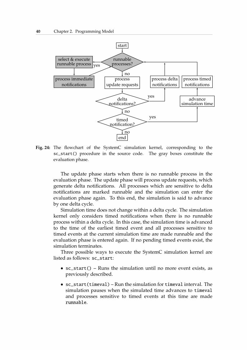
40 Chapter 2. Programming Model
start
select & executerunnable process
runnableprocesses?
process immediate
notifications
process
update requests
process delta
notifications
process timed
notifications
deltanotifications?
advancesimulation time
timednotification?
end
no
no
no
yes
yes
yes
Fig. 24: The flowchart of the SystemC simulation kernel, corresponding to the
sc_start() procedure in the source code. The gray boxes constitute the
evaluation phase.
The update phase starts when there is no runnable process in theevaluation phase. The update phase will process update requests, whichgenerate delta notifications. All processes which are sensitive to deltanotifications are marked runnable and the simulation can enter theevaluation phase again. To this end, the simulation is said to advanceby one delta cycle.
Simulation time does not change within a delta cycle. The simulationkernel only considers timed notifications when there is no runnableprocess within a delta cycle. In this case, the simulation time is advancedto the time of the earliest timed event and all processes sensitive totimed events at the current simulation time are made runnable and theevaluation phase is entered again. If no pending timed events exist, thesimulation terminates.
Three possible ways to execute the SystemC simulation kernel arelisted as follows: sc_start:
• sc_start() – Runs the simulation until no more event exists, aspreviously described.
• sc_start(timeval) – Run the simulation for timeval interval. Thesimulation pauses when the simulated time advances to timevaland processes sensitive to timed events at this time are maderunnable.
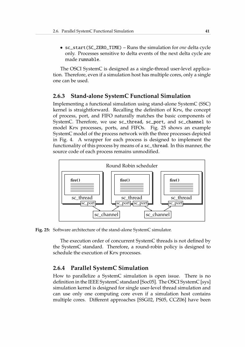
2.6. Parallel SystemC Functional Simulation 41
• sc_start(SC_ZERO_TIME) – Runs the simulation for one delta cycleonly. Processes sensitive to delta events of the next delta cycle aremade runnable.
The OSCI SystemC is designed as a single-thread user-level applica-tion. Therefore, even if a simulation host has multiple cores, only a singleone can be used.
2.6.3 Stand-alone SystemC Functional Simulation
Implementing a functional simulation using stand-alone SystemC (SSC)kernel is straightforward. Recalling the definition of Kpn, the conceptof process, port, and FIFO naturally matches the basic components ofSystemC. Therefore, we use sc_thread, sc_port, and sc_channel tomodel Kpn processes, ports, and FIFOs. Fig. 25 shows an exampleSystemCmodel of the process network with the three processes depictedin Fig. 4. A wrapper for each process is designed to implement thefunctionality of this process by means of a sc_thread. In this manner, thesource code of each process remains unmodified.
Round Robin scheduler
sc_thread
fire( )
sc_thread
fire( )
sc_thread
fire( )
sc_channel sc_channel
sc_port sc_port sc_port sc_port
Fig. 25: Software architecture of the stand-alone SystemC simulator.
The execution order of concurrent SystemC threads is not defined bythe SystemC standard. Therefore, a round-robin policy is designed toschedule the execution of Kpn processes.
2.6.4 Parallel SystemC Simulation
How to parallelize a SystemC simulation is open issue. There is nodefinition in the IEEE SystemC standard [Soc05]. TheOSCI SystemC [sys]simulation kernel is designed for single user-level thread simulation andcan use only one computing core even if a simulation host containsmultiple cores. Different approaches [SSG02, PS05, CCZ06] have been
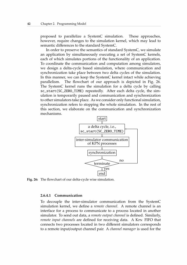
42 Chapter 2. Programming Model
proposed to parallelize a SystemC simulation. These approaches,however, require changes to the simulation kernel, which may lead tosemantic differences to the standard SystemC.
In order to preserve the semantics of standard SystemC, we simulatean application by simultaneously executing a set of SystemC kernels,each of which simulates portions of the functionality of an application.To coordinate the communication and computation among simulators,we design a delta-cycle based simulation, where communication andsynchronization take place between two delta cycles of the simulation.In this manner, we can keep the SystemC kernel intact while achievingparallelism. The flowchart of our approach is depicted in Fig. 26.The SystemC kernel runs the simulation for a delta cycle by callingsc_start(SC_ZERO_TIME) repeatedly. After each delta cycle, the sim-ulation is temporarily paused and communication and synchronizationto other simulators take place. Aswe consider only functional simulation,synchronization refers to stopping the whole simulation. In the rest ofthis section, we elaborate on the communication and synchronizationmechanisms.
start
a delta cycle, i.e.,sc_start(SC_ZERO_TIME)
inter-simulator communicationof KPN processes
synchronization
terminate
end
yes
no
Fig. 26: The flowchart of our delta-cycle wise simulation.
2.6.4.1 Communication
To decouple the inter-simulator communication from the SystemCsimulation kernel, we define a remote channel. A remote channel is aninterface for a process to communicate to a process located in anothersimulator. To send out data, a remote output channel is defined. Similarly,remote input channels are defined for receiving data. A Kpn FIFO thatconnects two processes located in two different simulators correspondsto a remote input/output channel pair. A channel manager is used for the
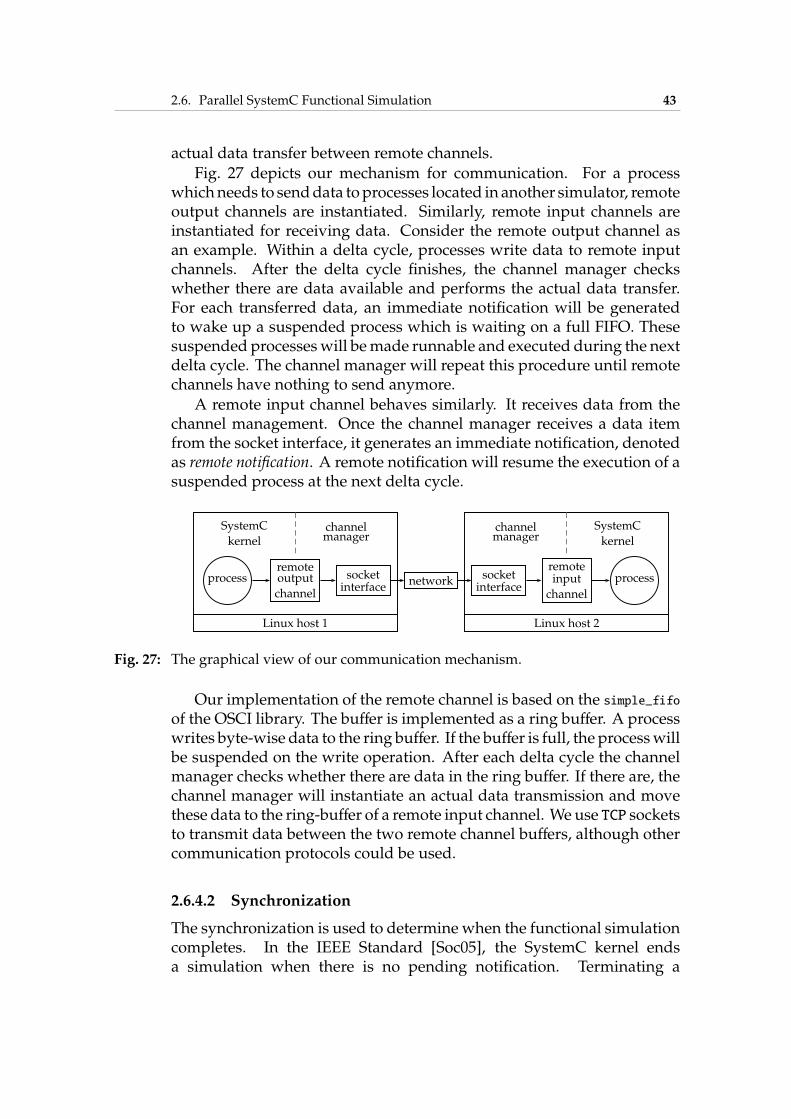
2.6. Parallel SystemC Functional Simulation 43
actual data transfer between remote channels.Fig. 27 depicts our mechanism for communication. For a process
whichneeds to senddata toprocesses located in another simulator, remoteoutput channels are instantiated. Similarly, remote input channels areinstantiated for receiving data. Consider the remote output channel asan example. Within a delta cycle, processes write data to remote inputchannels. After the delta cycle finishes, the channel manager checkswhether there are data available and performs the actual data transfer.For each transferred data, an immediate notification will be generatedto wake up a suspended process which is waiting on a full FIFO. Thesesuspended processeswill bemade runnable and executed during the nextdelta cycle. The channel manager will repeat this procedure until remotechannels have nothing to send anymore.
A remote input channel behaves similarly. It receives data from thechannel management. Once the channel manager receives a data itemfrom the socket interface, it generates an immediate notification, denotedas remote notification. A remote notification will resume the execution of asuspended process at the next delta cycle.
networksocket
interfacesocket
interface
remoteoutput
channel
remoteinput
channel
process process
Linux host 1 Linux host 2
SystemC
kernelchannelmanager
channelmanager
SystemC
kernel
Fig. 27: The graphical view of our communication mechanism.
Our implementation of the remote channel is based on the simple_fifoof the OSCI library. The buffer is implemented as a ring buffer. A processwrites byte-wise data to the ring buffer. If the buffer is full, the processwillbe suspended on the write operation. After each delta cycle the channelmanager checks whether there are data in the ring buffer. If there are, thechannel manager will instantiate an actual data transmission and movethese data to the ring-buffer of a remote input channel. We use TCP socketsto transmit data between the two remote channel buffers, although othercommunication protocols could be used.
2.6.4.2 Synchronization
The synchronization is used to determine when the functional simulationcompletes. In the IEEE Standard [Soc05], the SystemC kernel endsa simulation when there is no pending notification. Terminating a
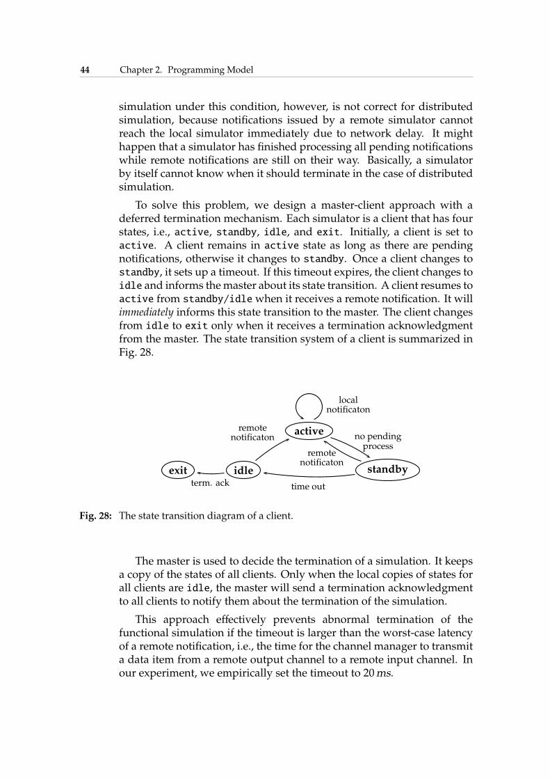
44 Chapter 2. Programming Model
simulation under this condition, however, is not correct for distributedsimulation, because notifications issued by a remote simulator cannotreach the local simulator immediately due to network delay. It mighthappen that a simulator has finished processing all pending notificationswhile remote notifications are still on their way. Basically, a simulatorby itself cannot know when it should terminate in the case of distributedsimulation.
To solve this problem, we design a master-client approach with adeferred termination mechanism. Each simulator is a client that has fourstates, i.e., active, standby, idle, and exit. Initially, a client is set toactive. A client remains in active state as long as there are pendingnotifications, otherwise it changes to standby. Once a client changes tostandby, it sets up a timeout. If this timeout expires, the client changes toidle and informs themaster about its state transition. A client resumes toactive from standby/idlewhen it receives a remote notification. It willimmediately informs this state transition to the master. The client changesfrom idle to exit only when it receives a termination acknowledgmentfrom the master. The state transition system of a client is summarized inFig. 28.
active
exit idle standby
no pendingprocess
remotenotificaton
time outterm. ack
remotenotificaton
localnotificaton
Fig. 28: The state transition diagram of a client.
The master is used to decide the termination of a simulation. It keepsa copy of the states of all clients. Only when the local copies of states forall clients are idle, the master will send a termination acknowledgmentto all clients to notify them about the termination of the simulation.
This approach effectively prevents abnormal termination of thefunctional simulation if the timeout is larger than the worst-case latencyof a remote notification, i.e., the time for the channel manager to transmita data item from a remote output channel to a remote input channel. Inour experiment, we empirically set the timeout to 20ms.
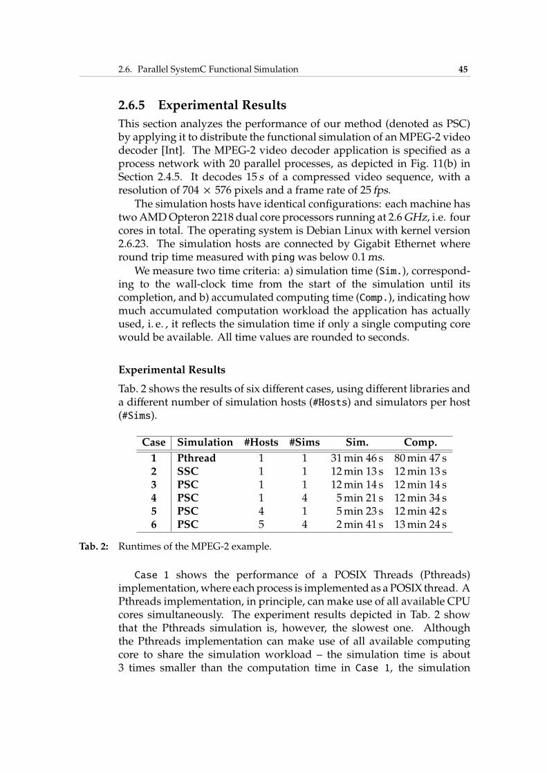
2.6. Parallel SystemC Functional Simulation 45
2.6.5 Experimental Results
This section analyzes the performance of our method (denoted as PSC)by applying it to distribute the functional simulation of anMPEG-2 videodecoder [Int]. The MPEG-2 video decoder application is specified as aprocess network with 20 parallel processes, as depicted in Fig. 11(b) inSection 2.4.5. It decodes 15 s of a compressed video sequence, with aresolution of 704 × 576 pixels and a frame rate of 25 fps.
The simulation hosts have identical configurations: each machine hastwoAMDOpteron 2218 dual core processors running at 2.6GHz, i.e. fourcores in total. The operating system is Debian Linux with kernel version2.6.23. The simulation hosts are connected by Gigabit Ethernet whereround trip time measured with ping was below 0.1ms.
We measure two time criteria: a) simulation time (Sim.), correspond-ing to the wall-clock time from the start of the simulation until itscompletion, and b) accumulated computing time (Comp.), indicating howmuch accumulated computation workload the application has actuallyused, i. e. , it reflects the simulation time if only a single computing corewould be available. All time values are rounded to seconds.
Experimental Results
Tab. 2 shows the results of six different cases, using different libraries anda different number of simulation hosts (#Hosts) and simulators per host(#Sims).
Case Simulation #Hosts #Sims Sim. Comp.
1 Pthread 1 1 31min 46 s 80min 47 s2 SSC 1 1 12min 13 s 12min 13 s3 PSC 1 1 12min 14 s 12min 14 s4 PSC 1 4 5min 21 s 12min 34 s5 PSC 4 1 5min 23 s 12min 42 s6 PSC 5 4 2min 41 s 13min 24 s
Tab. 2: Runtimes of the MPEG-2 example.
Case 1 shows the performance of a POSIX Threads (Pthreads)implementation,where eachprocess is implemented as aPOSIX thread. APthreads implementation, in principle, can make use of all available CPUcores simultaneously. The experiment results depicted in Tab. 2 showthat the Pthreads simulation is, however, the slowest one. Althoughthe Pthreads implementation can make use of all available computingcore to share the simulation workload – the simulation time is about3 times smaller than the computation time in Case 1, the simulation
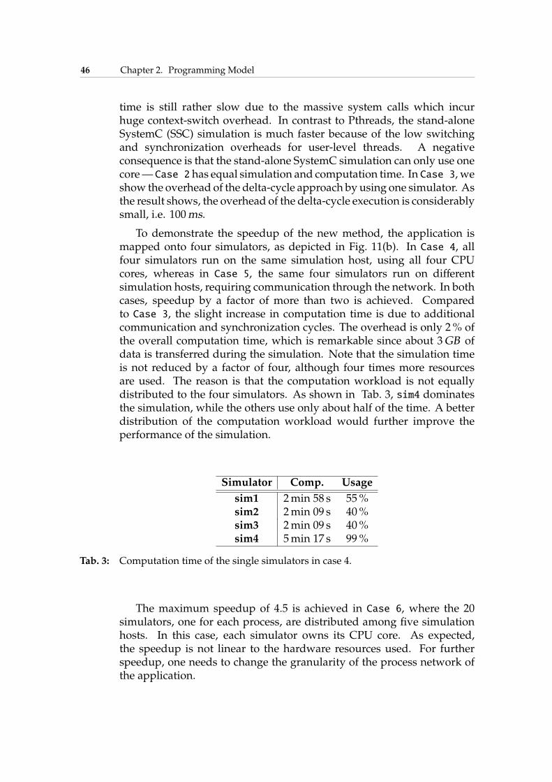
46 Chapter 2. Programming Model
time is still rather slow due to the massive system calls which incurhuge context-switch overhead. In contrast to Pthreads, the stand-aloneSystemC (SSC) simulation is much faster because of the low switchingand synchronization overheads for user-level threads. A negativeconsequence is that the stand-alone SystemC simulation can only use onecore— Case 2 has equal simulation and computation time. In Case 3, weshow the overhead of the delta-cycle approach by using one simulator. Asthe result shows, the overhead of the delta-cycle execution is considerablysmall, i.e. 100ms.
To demonstrate the speedup of the new method, the application ismapped onto four simulators, as depicted in Fig. 11(b). In Case 4, allfour simulators run on the same simulation host, using all four CPUcores, whereas in Case 5, the same four simulators run on differentsimulation hosts, requiring communication through the network. In bothcases, speedup by a factor of more than two is achieved. Comparedto Case 3, the slight increase in computation time is due to additionalcommunication and synchronization cycles. The overhead is only 2% ofthe overall computation time, which is remarkable since about 3GB ofdata is transferred during the simulation. Note that the simulation timeis not reduced by a factor of four, although four times more resourcesare used. The reason is that the computation workload is not equallydistributed to the four simulators. As shown in Tab. 3, sim4 dominatesthe simulation, while the others use only about half of the time. A betterdistribution of the computation workload would further improve theperformance of the simulation.
Simulator Comp. Usage
sim1 2min 58 s 55%sim2 2min 09 s 40%sim3 2min 09 s 40%sim4 5min 17 s 99%
Tab. 3: Computation time of the single simulators in case 4.
The maximum speedup of 4.5 is achieved in Case 6, where the 20simulators, one for each process, are distributed among five simulationhosts. In this case, each simulator owns its CPU core. As expected,the speedup is not linear to the hardware resources used. For furtherspeedup, one needs to change the granularity of the process network ofthe application.
2.7. Summary 47
2.7 Summary
In this chapter, we present a programmingmodel, suitable for developingstreaming multi/many-core embedded systems. Our programmingmodel follows the Y-chart paradigm, separating the concerns of appli-cation and architecture and of computation and communication. Forapplication modeling, we adopt the Kahn process network model ofcomputation. For specifying the application, architecture, mappingdescriptions, we design a hybrid programming syntax, i.e., C/C++/XML.To assist the design of future many-core embedded systems, an iteratortechnique is developed by which a specified system can be arbitrarilyscaled in a parametrizedmanner. To avoid the costly communication andsynchronization overhead incurred by large scale process networks, wepropose a variation of the FIFO syntax of Kpn, namely windowed FIFO.We also develop a distributed functional simulation as a proof-of-conceptruntime environment for our programmingmodel. The results presentedin this chapter lead to the free available embedded system software designtoolchain in [dol].
Our programming model specifies an embedded system at systemlevel, allowing a generic and versatile representation of a system. Theapplication specified in our programming model can be synthesized todifferent multi/many-core platforms. Platforms currently supported areIBMCell BroadbandEngine [HSH+09] (YellowDogLinux [yel] andGCC),ATMEL Shapeotto [HPB+] (DNA operating system [GP09] and C99), andMPARM [HHBT09b] (RTEMS real-time operating system [RTE] and C++).
Finally, our programming model offers more than programmabilityand scalability. In the next chapter, we present two performanceestimation techniques. Both of these techniques can be coupled to ourprogramming model and provide quantitative verifications for systemsspecified in our programing model.

48 Chapter 2. Programming Model
3Performance Evaluation
Performance is a prime metric in embedded system design as embeddedsystems are often subject to tight timing constraints such as throughput,latency, and response time. Analyzing timing behavior and reliablypredicting performance characteristics are essential to verify systemproperties and support important design decisions. Modern multi-coreand future many-core (often heterogeneous) architectures of embeddedsystems are, however, characterized by a large design space as thereis a large degree of freedom in the allocation of concurrent hardwarecomponents, the partitioning of parallel application tasks and theirbinding to hardware components, and the choice of appropriate resourceallocation schemes. Because of the overall system complexity, inspectingthe exact timing behavior of every design candidate of such an embeddedsystem is computationally prohibitive. Therefore, fast evaluationmethods in an early design stage are crucial for the exploration of thelarge design space.
Simulation-based methods for performance estimation are widelyused in industry. There are commercial tools such as Cadence VirtualComponent Co-design (VCC) [VCC] and CoWare Virtual Platform Ana-lyzer (VPA) [CoW], which support cycle/instruction-accurate simulationof complete HW/SW systems. Besides commercial tool suites, therealso exist open-source simulation frameworks that can be applied toperformance estimation, for instance, SystemC [sys]. Themain advantageof simulation-based approaches is their large and customizable modelingscope, which allows themodeling of systems at various abstraction levels.Simulation-based techniques, however, often suffer from long runtimesand high setup effort for each new architecture and mapping (process
50 Chapter 3. Performance Evaluation
allocation and scheduling discipline). Furthermore, worst-case boundson system properties like throughput and end-to-end delay cannot beobtained, in general, because of the exhaustive corner-case coveragecannot be guaranteed in simulation.
Formal analytic methods such as symbolic timing analysis forsystems (SymTA/S) [RE02], holistic analysis in the modeling and analysisfor systems (MAST) [PEP+04], and modular performance analysis(MPA) [TCN00, CKT03, WT06c], are viable alternatives, which provideexhaustive corner-case coverage and have a low setup effort. Therefore,to determine guaranteed performance limits, analytic methods arepreferable. The major disadvantage of analytic methods is that theytypically lack of effective ways to model complex interactions and state-dependent behavior, resulting in pessimistic bounds for certain scenarios.
The increasing number of integrated cores for future embeddedsystems accentuates the deficiencies of both simulation-based andanalytic approaches. In the case of simulations, the computing demandis super-linear to the number of cores to be simulated. In the caseof analytic methods, more cores involved result in more complexinteractions and correlations, which exceed themodeling scope of currentanalytic methods. The question hereby is how to accurately estimatethe performance for large-scale many-core embedded systems within areasonable time frame.
3.1 Overview
In this chapter, we investigate both analytic and simulation-basedtechniques for the performance estimation ofmulti/many-core embeddedsystems. In particular, we target streaming embedded systems thatexhibit complex interferences and correlations between data streams,computation, and communication. We present techniques to tackle thecomplex interference and correlations within these systems such thataccurate performance estimation can be conducted.
To analytically estimate the performance of a multi/many-core em-bedded system, we employ the modular performance analysis (MPA)framework [TCN00, CKT03, WT06c] that is based on real-time calculus(RTC). In Rtc-mpa, a system is decomposed into a network of abstractcomputation and communication components and is analyzed by theflow of event streams through this network of abstract components.The decompositional approach for performance analysis in Rtc-mpa,nevertheless, incurs an information loss among components. A typicalexample is that the timing correlations between event streams cannotbe effectively modeled, which leads to pessimistic analysis results. To
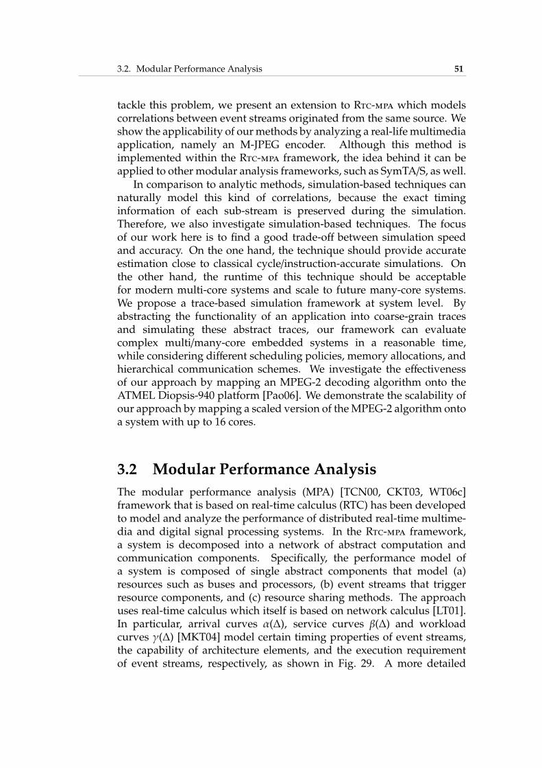
3.2. Modular Performance Analysis 51
tackle this problem, we present an extension to Rtc-mpa which modelscorrelations between event streams originated from the same source. Weshow the applicability of ourmethods by analyzing a real-life multimediaapplication, namely an M-JPEG encoder. Although this method isimplemented within the Rtc-mpa framework, the idea behind it can beapplied to other modular analysis frameworks, such as SymTA/S, as well.
In comparison to analytic methods, simulation-based techniques cannaturally model this kind of correlations, because the exact timinginformation of each sub-stream is preserved during the simulation.Therefore, we also investigate simulation-based techniques. The focusof our work here is to find a good trade-off between simulation speedand accuracy. On the one hand, the technique should provide accurateestimation close to classical cycle/instruction-accurate simulations. Onthe other hand, the runtime of this technique should be acceptablefor modern multi-core systems and scale to future many-core systems.We propose a trace-based simulation framework at system level. Byabstracting the functionality of an application into coarse-grain tracesand simulating these abstract traces, our framework can evaluatecomplex multi/many-core embedded systems in a reasonable time,while considering different scheduling policies, memory allocations, andhierarchical communication schemes. We investigate the effectivenessof our approach by mapping an MPEG-2 decoding algorithm onto theATMEL Diopsis-940 platform [Pao06]. We demonstrate the scalability ofour approach bymapping a scaled version of theMPEG-2 algorithm ontoa system with up to 16 cores.
3.2 Modular Performance Analysis
The modular performance analysis (MPA) [TCN00, CKT03, WT06c]framework that is based on real-time calculus (RTC) has been developedto model and analyze the performance of distributed real-time multime-dia and digital signal processing systems. In the Rtc-mpa framework,a system is decomposed into a network of abstract computation andcommunication components. Specifically, the performance model ofa system is composed of single abstract components that model (a)resources such as buses and processors, (b) event streams that triggerresource components, and (c) resource sharing methods. The approachuses real-time calculus which itself is based on network calculus [LT01].In particular, arrival curves α(∆), service curves β(∆) and workloadcurves γ(∆) [MKT04] model certain timing properties of event streams,the capability of architecture elements, and the execution requirementof event streams, respectively, as shown in Fig. 29. A more detailed

52 Chapter 3. Performance Evaluation
CPU CPU
EDFTDMA
α(∆)
γ(∆)
β(∆)
processnetwork
resourcesharing
executionplatform
Fig. 29: Elements of Rtc-mpa.
description of these elements is given in the following sections.
One drawback of using Rtc-mpa for performance analysis is that thedecomposition, nevertheless, leads to information loss. Considering asplit-join scenario that is typical for streaming applications, an inputstream is split into several sub-streams that will join again after beingprocessed separately. Obviously, the sub-streams are often highlycorrelated. Due to the decomposition in Rtc-mpa, these correlationscannot be effectively modeled. The phase information between the sub-streams with respect to the original input stream, for instance, is lostduring the analysis. In this work, we are interested in the correlationsin such a split-join scenario. We investigate techniques to model thecorrelations between streams that originate from the same input streamsuch that accurate performance analysis in terms of processing delaysand buffer space usage can be conducted.
3.2.1 Related Work
Although simulation-based methods are the most commonly usedtechniques for performance evaluation of embedded systems, formalanalytic methods are required, for instance, to determine guaranteedperformance limits and provide corner-case coverage These methodsprovide hard bounds that are needed to verify embedded systemswith respect to hard real-time requirements. In addition, performanceestimation using analyticmethods requires lower setup effort and smallercomputational demand,which is suitable for fast design space explorationat early design stages.
Several models and methods for analytic performance analysisof embedded systems have been developed. Holistic scheduling,
3.2. Modular Performance Analysis 53
for instance, extends well-known classical scheduling techniques todistributed systems [PGH98, TC94], combining the analysis of processorand bus scheduling. The modeling and analysis suite for real-timeapplications (MAST) [GHGGPGDM01] integrates a set of such holisticanalysis techniques. A more general approach to extend the conceptsof classical scheduling theory to distributed systems is presented in thesymbolic timing analysis of systems (SymTA/S) framework [RE02]. Incontrast to holistic approaches, this method applies existing analysistechniques in amodularmannerwhere single components of adistributedsystem are analyzed with classical algorithms, and the local results arepropagated through the system by appropriate interfaces relying on alimited set of event stream models. The modular performance analysis(MPA) framework [TCN00, CKT03, WT06c], which extends the basicconcepts of network calculus, presents a different analytic and modularapproach for performance analysis that does not rely on the classicalscheduling theory. It analyzes the flow of event streams through anetwork of computation and communication resources.
Thedisadvantage of analyticmethods is that they are typically not ableto model complex interactions and state-dependent behavior, resulting inpessimistic bounds for certain scenarios.
To achieve a shorter runtime in comparison to simulation-basedmethods and tighter performance bounds in comparison to analyticmethods, hybrid methods that combine simulation and analysis havebeen proposed. In [LRD01], a trace-based simulation method wasproposed, and in [KPBT06] a method is proposed to combine a SystemC-based cycle-accurate simulation [LAB+04] with an analytic technique[TCN00]. Although these hybrid methodologies can help to shorten theruntime of simulations, the problem of insufficient corner-case coverageis still present. Recently, a compositional and hybrid approach has beenpresented in [LPT09], which couples Rtc-mpa and state-based models inthe form of timed automata [AFM+02]. By defining a pattern to convertan abstract stream model, i. e. , periodic with jitter or time-interval basedmodels used in real-time calculus, to a network of co-operating timed-automata and vice versa, the proposed method enables a holistic analysisof a system composed of both MPA models and timed-automata.
In this section, we focus only on an analytic method, targeting thecorrelation between event streams. There are several approaches [JRE04,WT05] available to model event patterns and correlations within singleevent streams. In these approaches, models are developed to tacklecorrelations between different event types and workloads. None of theseexisting analytic approaches is able to model correlations between eventstreams, however. We present a method that can be used to analyze thecorrelation between different streams within a split-join scenario. By the
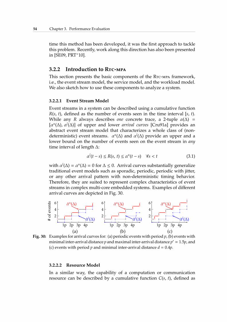
54 Chapter 3. Performance Evaluation
time this method has been developed, it was the first approach to tacklethis problem. Recently, work along this direction has also been presentedin [SE09, PRT+10].
3.2.2 Introduction to Rtc-mpa
This section presents the basic components of the Rtc-mpa framework,i.e., the event stream model, the service model, and the workload model.We also sketch how to use these components to analyze a system.
3.2.2.1 Event StreamModel
Event streams in a system can be described using a cumulative functionR(s, t), defined as the number of events seen in the time interval [s, t).While any R always describes one concrete trace, a 2-tuple α(∆) =[αu(∆), αl(∆)] of upper and lower arrival curves [Cru91a] provides anabstract event stream model that characterizes a whole class of (non-deterministic) event streams. αu(∆) and αl(∆) provide an upper and alower bound on the number of events seen on the event stream in anytime interval of length ∆:
αl(t − s) ≤ R(s, t) ≤ αu(t − s) ∀s < t (3.1)
with αl(∆) = αu(∆) = 0 for ∆ ≤ 0. Arrival curves substantially generalizetraditional event models such as sporadic, periodic, periodic with jitter,or any other arrival pattern with non-deterministic timing behavior.Therefore, they are suited to represent complex characteristics of eventstreams in complex multi-core embedded systems. Examples of differentarrival curves are depicted in Fig. 30.
2
4
6
1p 2p 3p 4p
bc bc
bc bc
bc bc
bc bc
bc bc
bc
r r
r r
r r
r r
r r
rαu(∆)
αl(∆)
(a)
#ofev
ents
2
4
6
1p 2p 3p 4p
bc bc
bc bc
bc bc
bc bc
bc bc
bc
r r
r r
r r
r r
αu(∆)
αl(∆)
(b)
2
4
6
1p 2p 3p 4p
bc bc
bc bc
bc bc
bc bc
bc bc
bc bc
bc
r r
r r
r r
r r
r r
rαu(∆)
αl(∆)
(c)Fig. 30: Examples for arrival curves for: (a) periodic events with period p, (b) events with
minimal inter-arrival distance p andmaximal inter-arrival distance p′ = 1.5p, and(c) events with period p and minimal inter-arrival distance d = 0.4p.
3.2.2.2 Resource Model
In a similar way, the capability of a computation or communicationresource can be described by a cumulative function C(s, t), defined as
3.2. Modular Performance Analysis 55
the number of available resources, e. g. , processor or bus cycles, in thetime interval [s, t). To provide an abstract resource model for a whole setof possible resource behavior, we define a 2-tuple β(∆) = [βu(∆), βl(∆)] ofupper and lower service curves:
βl(t − s) ≤ C(s, t) ≤ βu(t − s) ∀s < t (3.2)
with βl(∆) = βu(∆) = 0 for ∆ ≤ 0. Again, service curves substantiallygeneralize classical resource models such as the bounded delay or theperiodic resource model [SL04]. An example of the service curves for acommunication resource is shown in the following.
Ex. 2: Consider a bus with bandwidth B that implements the time division multipleaccess (TDMA) protocol. The length of individual TDMA slots is denoted bysi and the TDMA cycle length is denoted by c with c ≤
∑
si. Then, the servicecurves representing a slot are given as:
βli(∆) = B ·min{
⌈∆/c⌉ · si, ∆ − ⌊∆/c⌋ · (c − si)}
(3.3)
βui (∆) = B ·max{
⌊∆/c⌋ · si, ∆ − ⌈∆/c⌉ · (c − si)}
(3.4)
3.2.2.3 Workload Model
In the context of Rtc-mpa, the arrival curve is event-based whereas theservice curve is resource-based. To relate arrival and service curves,workload curves are used [MKT04]. The workload that an event streamimposes on a resource can be described by a cumulative functionW(s, t) defined as the number of clock cycles required to process events (included) to event t (excluded) – here we suppose that events aresuccessively numbered – on a computation or communication resource.We define a 2-tuple γ(∆) = [γu(∆), γl(∆)] of upper and lower workloadcurves:
γl(t − s) ≤W(s, t) ≤ γu(t − s) ∀s < t s, t ∈N0 (3.5)
Using the workload curve and its pseudo-inverse
(γu)−1(w) = sup{
e : γu(e) ≤ w}
(3.6)
(γl)−1(w) = inf{
e : γl(e) ≥ w}
(3.7)
arrival and service curves can be transformed from event-based toresource-based quantities and vice versa as follows:
αl(∆) = γl(
αl(∆))
βl(∆) = (γu)−1(
βl(∆))
(3.8)
αu(∆) = γu(
αu(∆))
βu(∆) = (γl)−1(
βu(∆))
(3.9)
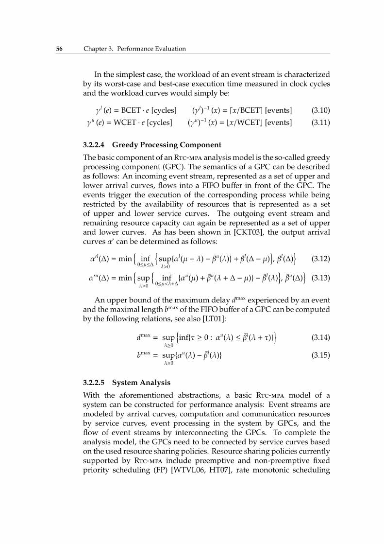
56 Chapter 3. Performance Evaluation
In the simplest case, the workload of an event stream is characterizedby its worst-case and best-case execution time measured in clock cyclesand the workload curves would simply be:
γl (e) = BCET · e [cycles] (γl)−1 (x) = ⌈x/BCET⌉ [events] (3.10)
γu (e) =WCET · e [cycles] (γu)−1 (x) = ⌊x/WCET⌋ [events] (3.11)
3.2.2.4 Greedy Processing Component
The basic component of an Rtc-mpa analysismodel is the so-called greedyprocessing component (GPC). The semantics of a GPC can be describedas follows: An incoming event stream, represented as a set of upper andlower arrival curves, flows into a FIFO buffer in front of the GPC. Theevents trigger the execution of the corresponding process while beingrestricted by the availability of resources that is represented as a setof upper and lower service curves. The outgoing event stream andremaining resource capacity can again be represented as a set of upperand lower curves. As has been shown in [CKT03], the output arrivalcurves α′ can be determined as follows:
α′l(∆) = min{
inf0≤µ≤∆
{
supλ>0
{αl(µ + λ) − βu(λ)} + βl(∆ − µ)}
, βl(∆)}
(3.12)
α′u(∆) = min{
supλ>0
{
inf0≤µ<λ+∆
{αu(µ) + βu(λ + ∆ − µ)} − βl(λ)}
, βu(∆)}
(3.13)
An upper bound of the maximum delay dmax experienced by an eventand themaximal length bmax of the FIFO buffer of a GPC can be computedby the following relations, see also [LT01]:
dmax = supλ≥0
{
inf{τ ≥ 0 : αu(λ) ≤ βl(λ + τ)}}
(3.14)
bmax = supλ≥0
{αu(λ) − βl(λ)} (3.15)
3.2.2.5 System Analysis
With the aforementioned abstractions, a basic Rtc-mpa model of asystem can be constructed for performance analysis: Event streams aremodeled by arrival curves, computation and communication resourcesby service curves, event processing in the system by GPCs, and theflow of event streams by interconnecting the GPCs. To complete theanalysis model, the GPCs need to be connected by service curves basedon the used resource sharing policies. Resource sharing policies currentlysupported by Rtc-mpa include preemptive and non-preemptive fixedpriority scheduling (FP) [WTVL06, HT07], rate monotonic scheduling
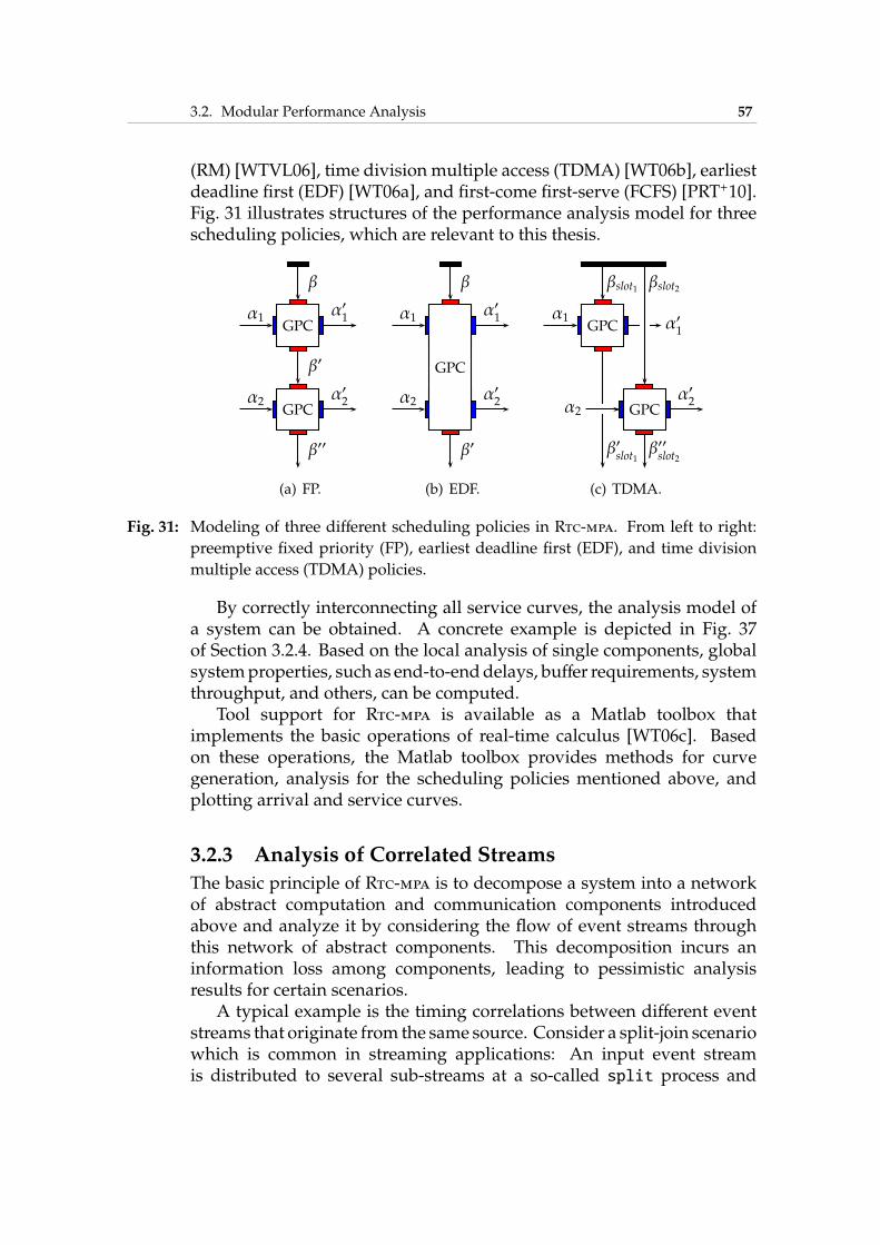
3.2. Modular Performance Analysis 57
(RM) [WTVL06], time division multiple access (TDMA) [WT06b], earliestdeadline first (EDF) [WT06a], and first-come first-serve (FCFS) [PRT+10].Fig. 31 illustrates structures of the performance analysis model for threescheduling policies, which are relevant to this thesis.
GPC
GPC
β
β′
β′′
α1 α′1
α2 α′2
(a) FP.
GPC
GPC
β
β′
α1 α′1
α2 α′2
GPC
(b) EDF.
GPCα1 α′
1
βslot1
β′slot1
GPCα2α′2
βslot2
β′′slot2
(c) TDMA.
Fig. 31: Modeling of three different scheduling policies in Rtc-mpa. From left to right:
preemptive fixed priority (FP), earliest deadline first (EDF), and time division
multiple access (TDMA) policies.
By correctly interconnecting all service curves, the analysis model ofa system can be obtained. A concrete example is depicted in Fig. 37of Section 3.2.4. Based on the local analysis of single components, globalsystemproperties, such as end-to-enddelays, buffer requirements, systemthroughput, and others, can be computed.
Tool support for Rtc-mpa is available as a Matlab toolbox thatimplements the basic operations of real-time calculus [WT06c]. Basedon these operations, the Matlab toolbox provides methods for curvegeneration, analysis for the scheduling policies mentioned above, andplotting arrival and service curves.
3.2.3 Analysis of Correlated Streams
The basic principle of Rtc-mpa is to decompose a system into a networkof abstract computation and communication components introducedabove and analyze it by considering the flow of event streams throughthis network of abstract components. This decomposition incurs aninformation loss among components, leading to pessimistic analysisresults for certain scenarios.
A typical example is the timing correlations between different eventstreams that originate from the same source. Consider a split-join scenariowhich is common in streaming applications: An input event streamis distributed to several sub-streams at a so-called split process and
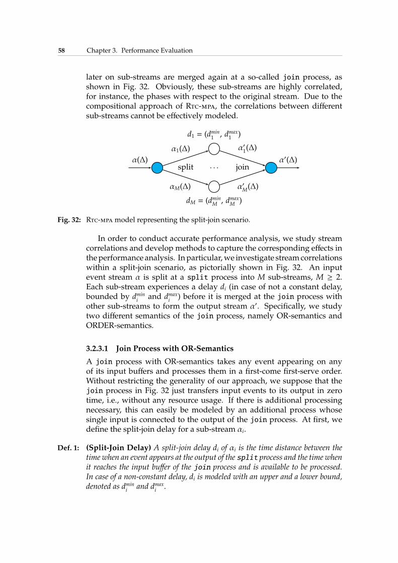
58 Chapter 3. Performance Evaluation
later on sub-streams are merged again at a so-called join process, asshown in Fig. 32. Obviously, these sub-streams are highly correlated,for instance, the phases with respect to the original stream. Due to thecompositional approach of Rtc-mpa, the correlations between differentsub-streams cannot be effectively modeled.
α1(∆)
αM(∆)
α′1(∆)
α′M(∆)
α(∆) α′(∆)
d1 = (dmin1, dmax
1)
dM = (dminM , d
maxM )
split join. . .
Fig. 32: Rtc-mpamodel representing the split-join scenario.
In order to conduct accurate performance analysis, we study streamcorrelations and develop methods to capture the corresponding effects intheperformance analysis. Inparticular,we investigate streamcorrelationswithin a split-join scenario, as pictorially shown in Fig. 32. An inputevent stream α is split at a split process into M sub-streams, M ≥ 2.Each sub-stream experiences a delay di (in case of not a constant delay,bounded by dmin
iand dmax
i) before it is merged at the join process with
other sub-streams to form the output stream α′. Specifically, we studytwo different semantics of the join process, namely OR-semantics andORDER-semantics.
3.2.3.1 Join Process with OR-Semantics
A join process with OR-semantics takes any event appearing on anyof its input buffers and processes them in a first-come first-serve order.Without restricting the generality of our approach, we suppose that thejoin process in Fig. 32 just transfers input events to its output in zerotime, i.e., without any resource usage. If there is additional processingnecessary, this can easily be modeled by an additional process whosesingle input is connected to the output of the join process. At first, wedefine the split-join delay for a sub-stream αi.
Def. 1: (Split-Join Delay) A split-join delay di of αi is the time distance between thetime when an event appears at the output of the split process and the time whenit reaches the input buffer of the join process and is available to be processed.In case of a non-constant delay, di is modeled with an upper and a lower bound,denoted as dmin
iand dmax
i.
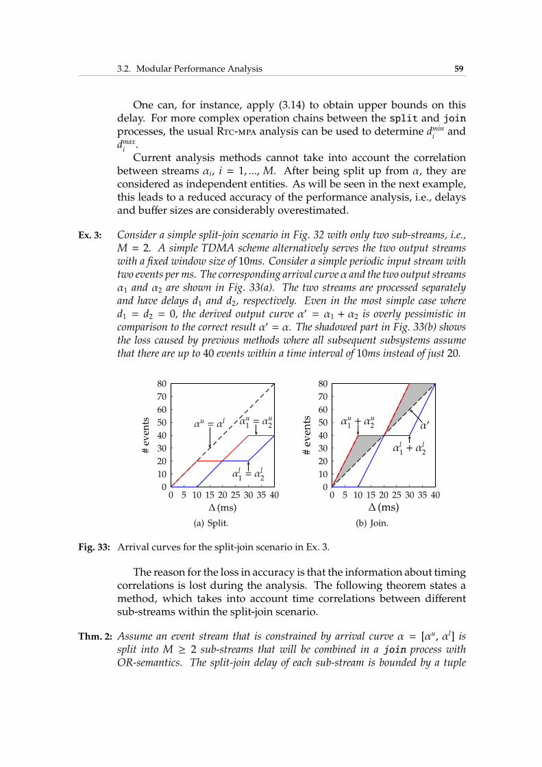
3.2. Modular Performance Analysis 59
One can, for instance, apply (3.14) to obtain upper bounds on thisdelay. For more complex operation chains between the split and joinprocesses, the usual Rtc-mpa analysis can be used to determine dmin
iand
dmaxi
.Current analysis methods cannot take into account the correlation
between streams αi, i = 1, ..., M. After being split up from α, they areconsidered as independent entities. As will be seen in the next example,this leads to a reduced accuracy of the performance analysis, i.e., delaysand buffer sizes are considerably overestimated.
Ex. 3: Consider a simple split-join scenario in Fig. 32 with only two sub-streams, i.e.,M = 2. A simple TDMA scheme alternatively serves the two output streamswith a fixed window size of 10ms. Consider a simple periodic input stream withtwo events perms. The corresponding arrival curveα and the two output streamsα1 and α2 are shown in Fig. 33(a). The two streams are processed separatelyand have delays d1 and d2, respectively. Even in the most simple case whered1 = d2 = 0, the derived output curve α′ = α1 + α2 is overly pessimistic incomparison to the correct result α′ = α. The shadowed part in Fig. 33(b) showsthe loss caused by previous methods where all subsequent subsystems assumethat there are up to 40 events within a time interval of 10ms instead of just 20.
0
10
20
30
40
50
60
70
80
0 5 10 15 20 25 30 35 40
#ev
ents
∆ (ms)
αu1= αu
2
αl1= αl
2
αu = αl
(a) Split.
0
10
20
30
40
50
60
70
80
0 5 10 15 20 25 30 35 40
#ev
ents
∆ (ms)
αu1+ αu2
αl1+ αl2
α′
(b) Join.
Fig. 33: Arrival curves for the split-join scenario in Ex. 3.
The reason for the loss in accuracy is that the information about timingcorrelations is lost during the analysis. The following theorem states amethod, which takes into account time correlations between differentsub-streams within the split-join scenario.
Thm. 2: Assume an event stream that is constrained by arrival curve α = [αu, αl] issplit into M ≥ 2 sub-streams that will be combined in a join process withOR-semantics. The split-join delay of each sub-stream is bounded by a tuple
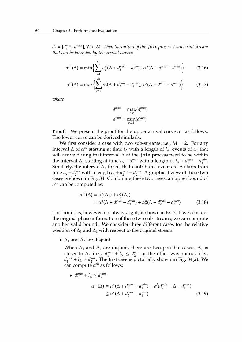
60 Chapter 3. Performance Evaluation
di = [dmini, dmax
i], ∀i ∈M. Then the output of the join process is an event stream
that can be bounded by the arrival curves
α′u(∆) =min{ M∑
i=1
αui (∆ + dmaxi − dmin
i ), αu(∆ + dmax − dmin)}
(3.16)
α′l(∆) =max{ M∑
i=1
αli(∆ + dmini − dmax
i ), αl(∆ + dmin − dmax)}
(3.17)
where
dmax = maxi∈M{dmax
i }
dmin = mini∈M{dmin
i }
Proof. We present the proof for the upper arrival curve α′u as follows.The lower curve can be derived similarly.
We first consider a case with two sub-streams, i.e., M = 2. For anyinterval ∆ of α′u starting at time t∆ with a length of l∆, events of α1 thatwill arrive during that interval ∆ at the join process need to be withinthe interval ∆1 starting at time t∆ − dmax
1with a length of l∆ + dmax
1− dmin
1.
Similarly, the interval ∆2 for α2 that contributes events to ∆ starts fromtime t∆ − d
max2 with a length l∆ + d
max2 − dmin
2 . A graphical view of these twocases is shown in Fig. 34. Combining these two cases, an upper bound ofα′u can be computed as:
α′u(∆) = αu1(∆1) + αu2(∆2)
= αu1(∆ + dmax1 − dmin
1 ) + αu2(∆ + dmax2 − dmin
2 ) (3.18)
This bound is, however, not always tight, as shown in Ex. 3. Ifwe considerthe original phase information of these two sub-streams, we can computeanother valid bound. We consider three different cases for the relativeposition of ∆1 and ∆2 with respect to the original stream:
• ∆1 and ∆2 are disjoint.
When ∆1 and ∆2 are disjoint, there are two possible cases: ∆1 iscloser to ∆, i. e. , dmax
1+ l∆ ≤ dmin
2 or the other way round, i. e. ,dmax1+ l∆ > dmin
2 . The first case is pictorially shown in Fig. 34(a). Wecan compute α′u as follows:
◮ dmax1+ l∆ ≤ dmin
2
α′u(∆) = αu(∆ + dmax2 − dmin
1 ) − αl(dmin2 − ∆ − dmax
1 )
≤ αu(∆ + dmax2 − dmin
1 ) (3.19)
3.2. Modular Performance Analysis 61
◮ dmax1+ l∆ > dmin
2
α′u(∆) = αu(∆ + dmax1 − dmin
2 ) − αl(dmin1 − ∆ − dmax
2 )
≤ αu(∆ + dmax1 − dmin
2 ) (3.20)
• ∆1 and ∆2 intersect.
When ∆1 and ∆2 intersect, there are again two cases: ∆1 is closerto ∆, i. e. , dmin
1< dmin
2 < dmax1+ l∆ or the other way round, i. e. ,
dmin2 < dmin
1< dmax
2 + l∆. Fig. 34(b) again shows the first case in which∆1 is closer to ∆. We compute α′u as follows:
◮ dmin1< dmin
2 < dmax1+ l∆
α′u(∆) = αu(∆ + dmax2 − dmin
1 ) (3.21)
◮ dmin2 < dmin
1< dmax
2 + l∆
α′u(∆) = αu(∆ + dmax1 − dmin
2 ) (3.22)
• One of ∆1 and ∆2 completely overlaps the other.
For the case of a complete overlap, we again have two cases: ∆1
overlaps ∆2, i. e. , dmin2 ≤ dmin
1and dmax
2 ≥ dmax1
or the other wayround, i. e. , dmin
1≤ dmin
2 and dmax1≥ dmax
2 . Fig. 34(c) shows the firstcase in which ∆1 overlaps ∆2. We derive α′u as follows:
◮ dmin2 ≤ dmin
1and dmax
2 ≥ dmax1
α′u(∆) = αu(∆ + dmax2 − dmin
2 ) (3.23)
◮ dmin1≤ dmin
2 and dmax1≥ dmax
2
α′u(∆) = αu(∆ + dmax1 − dmin
1 ) (3.24)
Combining (3.19)–(3.24), we have
α′u(∆) = αu(∆ + dmax − dmin) (3.25)
where dmax = max{dmax1, dmax
2 } and dmin = min{dmin1, dmin
2 }. The computed α′u
from (3.25) is also a valid upper bound for α′u. With (3.18) and (3.25), wehave
α′u(∆) = min{ 2∑
i=1
αui (∆ + dmaxi − dmin
i ), αu(∆ + dmax − dmin)}
(3.26)
Therefore, the theorem holds for M = 2.
62 Chapter 3. Performance Evaluation
t∆
t∆
∆1
∆2
dmin1
dmax1
dmin2
dmax2
(a) ∆1 and ∆2 are disjoint.
t∆
t∆
∆1
∆2
dmin1
dmax1
dmin2
dmax2
(b) ∆1 and ∆2 intersect.
t∆
t⊥∆
∆1
∆2
dmin1
dmax1
dmin2
dmax2
(c) ∆2 overlaps ∆1.
Fig. 34: Illustration for the proof of Theorem 2 in the case ofM = 2.
For cases M > 2, the proof is similar to M = 2. For each ∆ of α′u, wecan always compute ∆i for αi, i ∈ M. Moreover, based on enumerationssimilar to (3.19)–(3.24), the computed∆+dmax−dmin defines another upperbound for the interval inwhich events from the original streamwill arrivewithin ∆ of α′u. Therefore, the theorem holds.
�
3.2.3.2 Join Process with ORDER-Semantics
In OR-semantics, the join process greedily takes events from any of itsinputs whenever events are available. Thus, the order of events withrespect to the one in the original stream α is not guaranteed. Preservingthe order of events in α′ with respect to α is, however, necessary forcertain cases of streaming applications, e. g. , video codec applications.
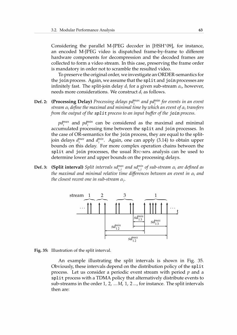
3.2. Modular Performance Analysis 63
Considering the parallel M-JPEG decoder in [HSH+09], for instance,an encoded M-JPEG video is dispatched frame-by-frame to differenthardware components for decompression and the decoded frames arecollected to form a video stream. In this case, preserving the frame orderis mandatory in order not to scramble the resulted video.
To preserve the original order, we investigate anORDER-semantics forthe joinprocess. Again, we assume that the split and joinprocesses areinfinitely fast. The split-join delay di for a given sub-stream αi, however,needs more considerations. We construct di as follows.
Def. 2: (Processing Delay) Processing delays pdmaxi
and pdmini
for events in an eventstream αi define the maximal and minimal time by which an event of αi transfersfrom the output of the split process to an input buffer of the join process.
pdmaxi
and pdmini
can be considered as the maximal and minimalaccumulated processing time between the split and join processes. Inthe case of OR-semantics for the join process, they are equal to the split-join delays dmax
iand dmin
i. Again, one can apply (3.14) to obtain upper
bounds on this delay. For more complex operation chains between thesplit and join processes, the usual Rtc-mpa analysis can be used todetermine lower and upper bounds on the processing delays.
Def. 3: (Split interval) Split intervals sdmaxi, j and sdmin
i, j of sub-stream αi are defined as
the maximal and minimal relative time differences between an event in αi andthe closest recent one in sub-stream α j.
t. . .
stream︷︸︸︷1︷︸︸︷2
︷ ︸︸ ︷3
︷ ︸︸ ︷1
. . .
sdmax1 2
sdmin1 2
sdmin1 3
sdmax1 3
Fig. 35: Illustration of the split interval.
An example illustrating the split intervals is shown in Fig. 35.Obviously, these intervals depend on the distribution policy of the splitprocess. Let us consider a periodic event stream with period p and asplit process with a TDMA policy that alternatively distribute events tosub-streams in the order 1, 2, ...M, 1, 2 ..., for instance. The split intervalsthen are:
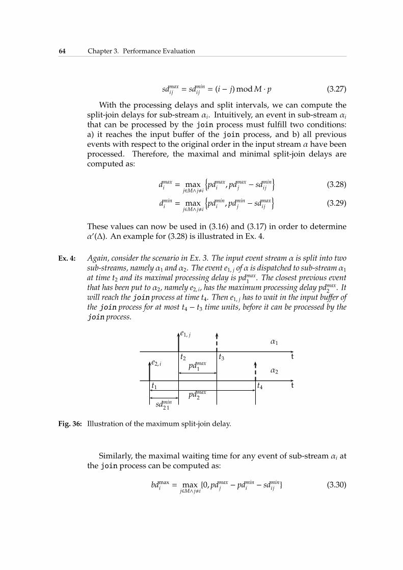
64 Chapter 3. Performance Evaluation
sdmaxij = sdmin
ij = (i − j)modM · p (3.27)
With the processing delays and split intervals, we can compute thesplit-join delays for sub-stream αi. Intuitively, an event in sub-stream αithat can be processed by the join process must fulfill two conditions:a) it reaches the input buffer of the join process, and b) all previousevents with respect to the original order in the input stream α have beenprocessed. Therefore, the maximal and minimal split-join delays arecomputed as:
dmaxi = max
j∈M∧ j,i
{
pdmaxi , pd
maxj − sdmin
ij
}
(3.28)
dmini = max
j∈M∧ j,i
{
pdmini , pd
minj − sdmax
ij
}
(3.29)
These values can now be used in (3.16) and (3.17) in order to determineα′(∆). An example for (3.28) is illustrated in Ex. 4.
Ex. 4: Again, consider the scenario in Ex. 3. The input event stream α is split into twosub-streams, namely α1 and α2. The event e1, j of α is dispatched to sub-stream α1at time t2 and its maximal processing delay is pdmax
1. The closest previous event
that has been put to α2, namely e2, i, has the maximum processing delay pdmax2 . It
will reach the join process at time t4. Then e1, j has to wait in the input buffer ofthe join process for at most t4 − t3 time units, before it can be processed by thejoin process.
t
t
α1
α2e2, i
t1 t4
e1, j
t2 t3
sdmin2 1
pdmax2
pdmax1
Fig. 36: Illustration of the maximum split-join delay.
Similarly, the maximal waiting time for any event of sub-stream αi atthe join process can be computed as:
bdmaxi = max
j∈M∧ j,i{0, pdmax
j − pdmini − sdmin
ij } (3.30)
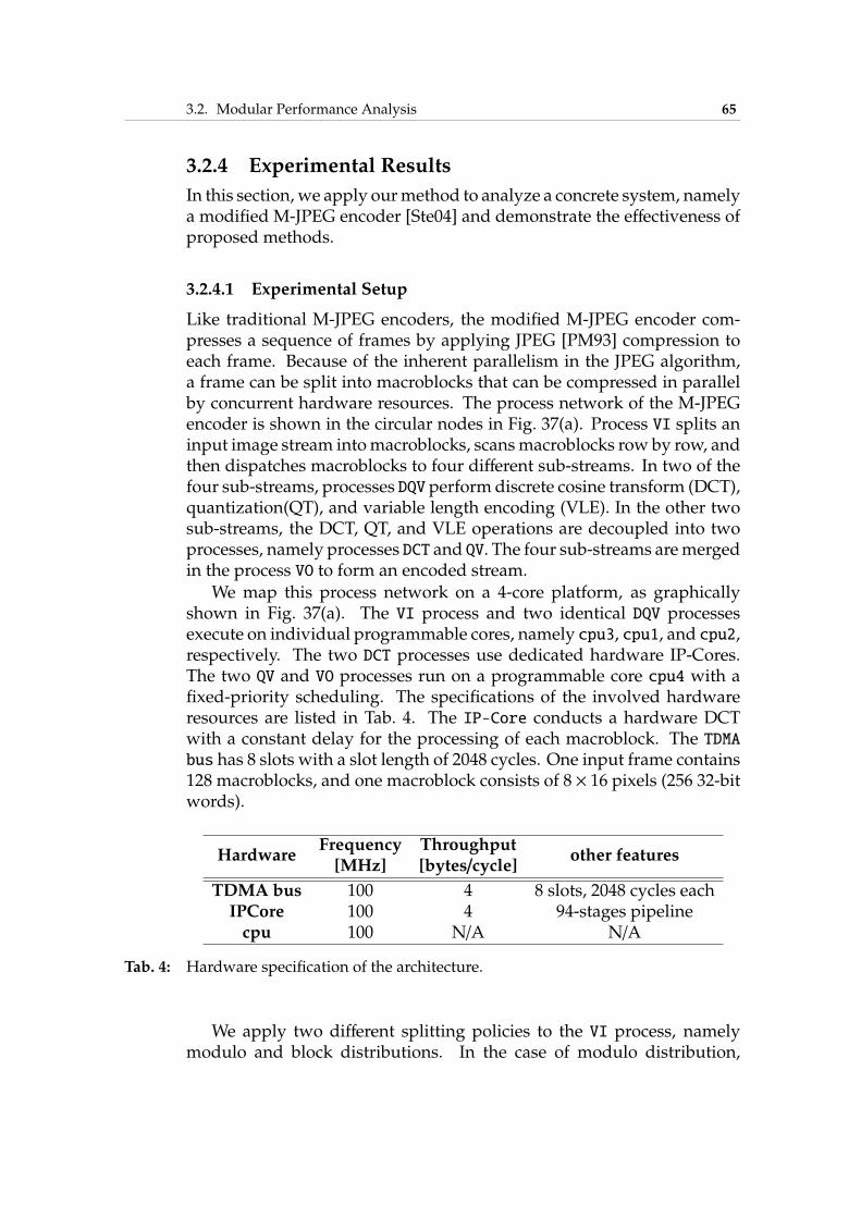
3.2. Modular Performance Analysis 65
3.2.4 Experimental Results
In this section, we apply ourmethod to analyze a concrete system, namelya modified M-JPEG encoder [Ste04] and demonstrate the effectiveness ofproposed methods.
3.2.4.1 Experimental Setup
Like traditional M-JPEG encoders, the modified M-JPEG encoder com-presses a sequence of frames by applying JPEG [PM93] compression toeach frame. Because of the inherent parallelism in the JPEG algorithm,a frame can be split into macroblocks that can be compressed in parallelby concurrent hardware resources. The process network of the M-JPEGencoder is shown in the circular nodes in Fig. 37(a). Process VI splits aninput image stream intomacroblocks, scansmacroblocks row by row, andthen dispatches macroblocks to four different sub-streams. In two of thefour sub-streams, processes DQV perform discrete cosine transform (DCT),quantization(QT), and variable length encoding (VLE). In the other twosub-streams, the DCT, QT, and VLE operations are decoupled into twoprocesses, namely processes DCT and QV. The four sub-streams aremergedin the process VO to form an encoded stream.
We map this process network on a 4-core platform, as graphicallyshown in Fig. 37(a). The VI process and two identical DQV processesexecute on individual programmable cores, namely cpu3, cpu1, and cpu2,respectively. The two DCT processes use dedicated hardware IP-Cores.The two QV and VO processes run on a programmable core cpu4 with afixed-priority scheduling. The specifications of the involved hardwareresources are listed in Tab. 4. The IP-Core conducts a hardware DCTwith a constant delay for the processing of each macroblock. The TDMAbus has 8 slots with a slot length of 2048 cycles. One input frame contains128 macroblocks, and one macroblock consists of 8 × 16 pixels (256 32-bitwords).
HardwareFrequency Throughput
other features[MHz] [bytes/cycle]
TDMA bus 100 4 8 slots, 2048 cycles eachIPCore 100 4 94-stages pipelinecpu 100 N/A N/A
Tab. 4: Hardware specification of the architecture.
We apply two different splitting policies to the VI process, namelymodulo and block distributions. In the case of modulo distribution,
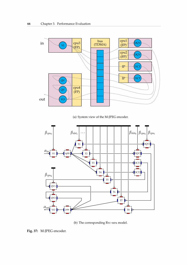
66 Chapter 3. Performance Evaluation
VIDQV
DQV
DCT
DCTQV
QV
VO
in
out
bus(TDMA)
cpu4
(FP)
cpu3
(FP)
cpu1
(FP)
cpu2
(FP)
IP
IP
(a) System view of the M-JPEG encoder.
VI split
QV1
QV2
VO join
T1
T2
T3
T4
T5
T6
T7
T8
DQV1
DQV2
DCT1
DCT2
βslot1 . . . βslot8
βcpu4
βcpu3 βcpu1βcpu2
αin
αout
(b) The corresponding Rtc-mpamodel.
Fig. 37: M-JPEG encoder.
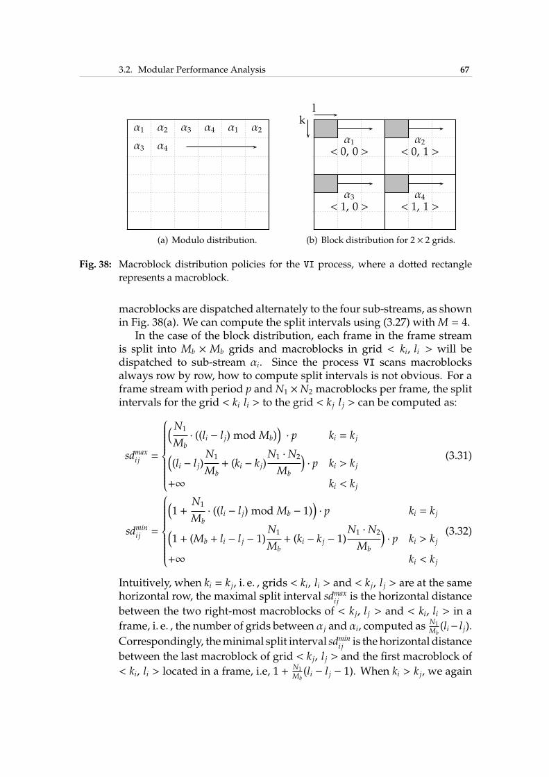
3.2. Modular Performance Analysis 67
α1 α2 α3 α4 α1 α2
α3 α4
(a) Modulo distribution.
kl
α1< 0, 0 >
α2< 0, 1 >
α3< 1, 0 >
α4< 1, 1 >
(b) Block distribution for 2 × 2 grids.
Fig. 38: Macroblock distribution policies for the VI process, where a dotted rectangle
represents a macroblock.
macroblocks are dispatched alternately to the four sub-streams, as shownin Fig. 38(a). We can compute the split intervals using (3.27) withM = 4.
In the case of the block distribution, each frame in the frame streamis split into Mb × Mb grids and macroblocks in grid < ki, li > will bedispatched to sub-stream αi. Since the process VI scans macroblocksalways row by row, how to compute split intervals is not obvious. For aframe stream with period p and N1 ×N2 macroblocks per frame, the splitintervals for the grid < ki li > to the grid < k j l j > can be computed as:
sdmaxij =
(N1
Mb· ((li − l j) mod Mb)
)
· p ki = k j
(
(li − l j)N1
Mb+ (ki − k j)
N1 ·N2
Mb
)
· p ki > k j
+∞ ki < k j
(3.31)
sdminij =
(
1 +N1
Mb· ((li − l j) mod Mb − 1)
)
· p ki = k j
(
1 + (Mb + li − l j − 1)N1
Mb+ (ki − k j − 1)
N1 ·N2
Mb
)
· p ki > k j
+∞ ki < k j
(3.32)
Intuitively, when ki = k j, i. e. , grids < ki, li > and < k j, l j > are at the samehorizontal row, the maximal split interval sdmax
ijis the horizontal distance
between the two right-most macroblocks of < k j, l j > and < ki, li > in a
frame, i. e. , the number of grids between α j and αi, computed as N1
Mb(li− l j).
Correspondingly, theminimal split interval sdminij
is the horizontal distance
between the last macroblock of grid < k j, l j > and the first macroblock of
< ki, li > located in a frame, i.e, 1 + N1
Mb(li − l j − 1). When ki > k j, we again
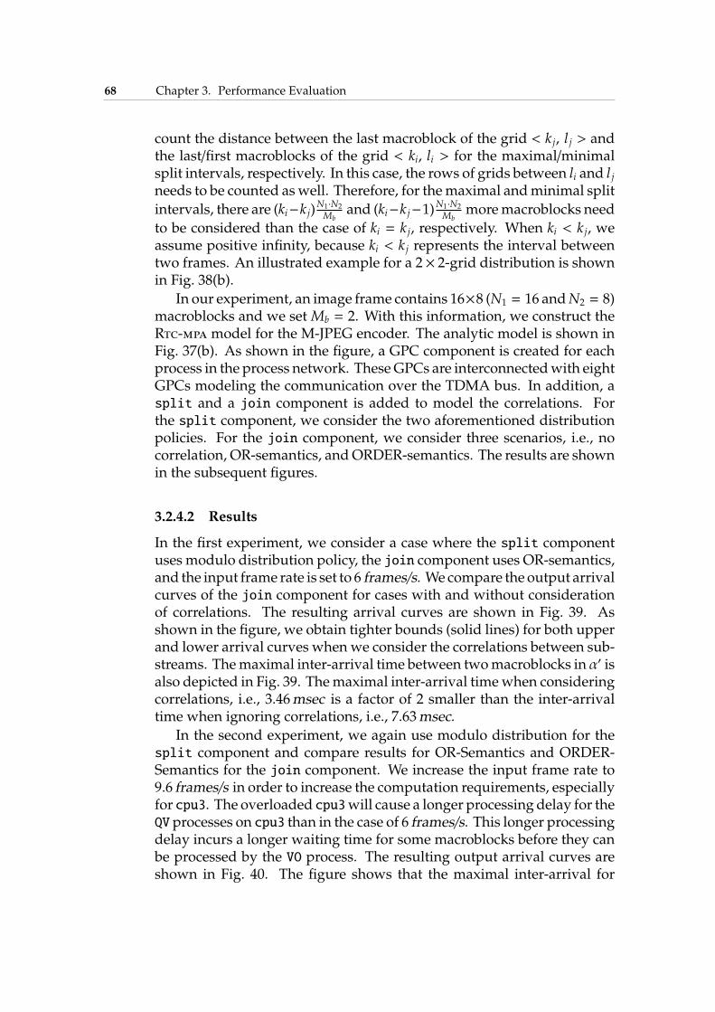
68 Chapter 3. Performance Evaluation
count the distance between the last macroblock of the grid < k j, l j > andthe last/first macroblocks of the grid < ki, li > for the maximal/minimalsplit intervals, respectively. In this case, the rows of grids between li and l jneeds to be counted aswell. Therefore, for themaximal andminimal split
intervals, there are (ki−k j)N1·N2
Mband (ki−k j−1)
N1·N2
Mbmoremacroblocks need
to be considered than the case of ki = k j, respectively. When ki < k j, weassume positive infinity, because ki < k j represents the interval betweentwo frames. An illustrated example for a 2× 2-grid distribution is shownin Fig. 38(b).
In our experiment, an image frame contains 16×8 (N1 = 16 andN2 = 8)macroblocks and we set Mb = 2. With this information, we construct theRtc-mpa model for the M-JPEG encoder. The analytic model is shown inFig. 37(b). As shown in the figure, a GPC component is created for eachprocess in the process network. TheseGPCs are interconnectedwith eightGPCs modeling the communication over the TDMA bus. In addition, asplit and a join component is added to model the correlations. Forthe split component, we consider the two aforementioned distributionpolicies. For the join component, we consider three scenarios, i.e., nocorrelation, OR-semantics, andORDER-semantics. The results are shownin the subsequent figures.
3.2.4.2 Results
In the first experiment, we consider a case where the split componentuses modulo distribution policy, the join component uses OR-semantics,and the input frame rate is set to 6 frames/s. We compare the output arrivalcurves of the join component for cases with and without considerationof correlations. The resulting arrival curves are shown in Fig. 39. Asshown in the figure, we obtain tighter bounds (solid lines) for both upperand lower arrival curves when we consider the correlations between sub-streams. Themaximal inter-arrival time between twomacroblocks in α′ isalso depicted in Fig. 39. Themaximal inter-arrival timewhen consideringcorrelations, i.e., 3.46msec is a factor of 2 smaller than the inter-arrivaltime when ignoring correlations, i.e., 7.63msec.
In the second experiment, we again use modulo distribution for thesplit component and compare results for OR-Semantics and ORDER-Semantics for the join component. We increase the input frame rate to9.6 frames/s in order to increase the computation requirements, especiallyfor cpu3. The overloaded cpu3will cause a longer processing delay for theQV processes on cpu3 than in the case of 6 frames/s. This longer processingdelay incurs a longer waiting time for some macroblocks before they canbe processed by the VO process. The resulting output arrival curves areshown in Fig. 40. The figure shows that the maximal inter-arrival for
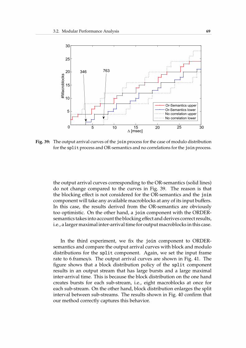
3.2. Modular Performance Analysis 69
∆ [msec]
# M
acro
blo
cks
0 5 10 15 20 25 30
5
10
15
20
25
30
346 763
Or-Semantics upper
Or-Semantics lowerNo correlation upper
No correlation lower
Fig. 39: The output arrival curves of the join process for the case of modulo distribution
for the split process andOR-semantics and no correlations for the join process.
the output arrival curves corresponding to the OR-semantics (solid lines)do not change compared to the curves in Fig. 39. The reason is thatthe blocking effect is not considered for the OR-semantics and the joincomponent will take any availablemacroblocks at any of its input buffers.In this case, the results derived from the OR-semantics are obviouslytoo optimistic. On the other hand, a join component with the ORDER-semantics takes into account theblocking effect andderives correct results,i.e., a largermaximal inter-arrival time for outputmacroblocks in this case.
In the third experiment, we fix the join component to ORDER-semantics and compare the output arrival curves with block and modulodistributions for the split component. Again, we set the input framerate to 6 frames/s. The output arrival curves are shown in Fig. 41. Thefigure shows that a block distribution policy of the split componentresults in an output stream that has large bursts and a large maximalinter-arrival time. This is because the block distribution on the one handcreates bursts for each sub-stream, i.e., eight macroblocks at once foreach sub-stream. On the other hand, block distribution enlarges the splitinterval between sub-streams. The results shown in Fig. 40 confirm thatour method correctly captures this behavior.
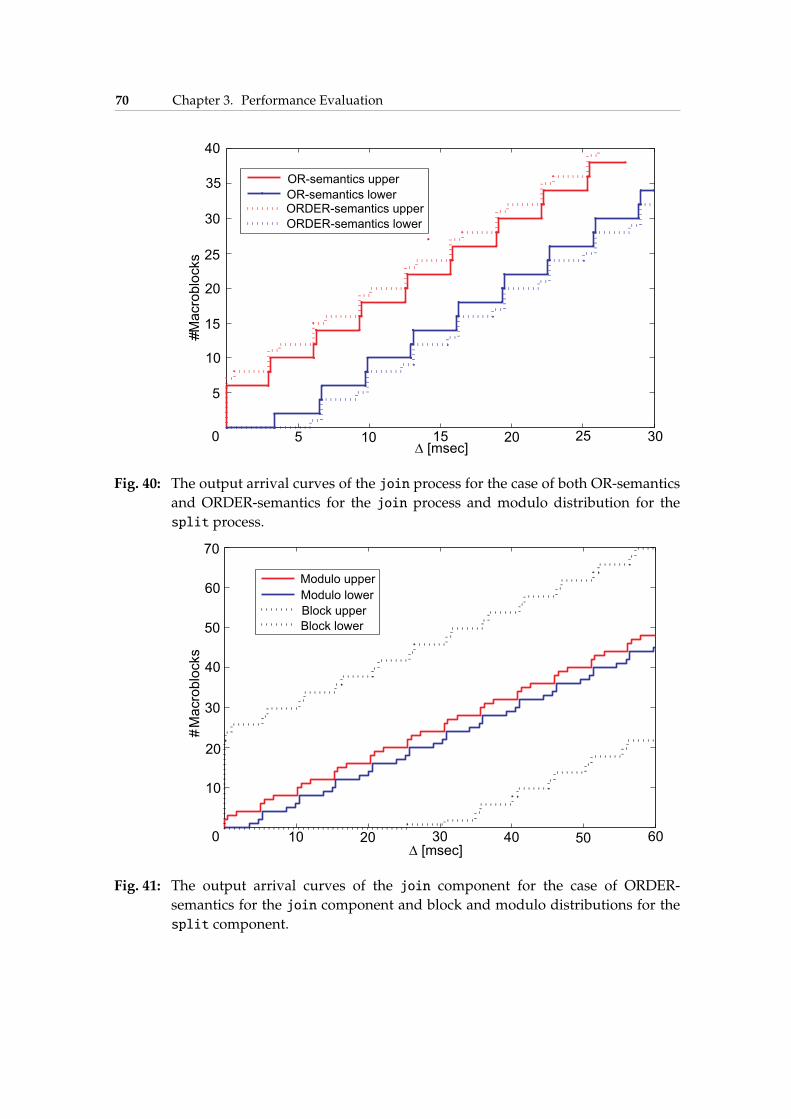
70 Chapter 3. Performance Evaluation
# M
acro
blo
cks
∆ [msec]0 5 10 15 20 25 30
5
10
15
20
25
30
OR-semantics upper
OR-semantics lowerORDER-semantics upper
ORDER-semantics lower
35
40
Fig. 40: The output arrival curves of the join process for the case of both OR-semantics
and ORDER-semantics for the join process and modulo distribution for the
split process.
# M
acro
blo
cks
∆ [msec]0 10 20 30 40 50 60
10
20
30
40
50
60
70
Modulo upper
Modulo lower
Block upper
Block lower
Fig. 41: The output arrival curves of the join component for the case of ORDER-
semantics for the join component and block and modulo distributions for the
split component.
3.3. Trace-Based Simulation 71
3.3 Trace-Based Simulation
To model and analyze the complex interference and correlations betweendata streams, simulation-based approaches can be used as well. Becausethe exact timing information of each sub-stream is preserved during thesimulation, the interference and correlations can be captured more natu-rally. Although simulation-based techniques cannot provide guaranteedbounds on system properties, they can be used to estimate average-caseperformance and to inspect properties at lower abstraction levels thatanalytic methods cannot capture. Therefore, we exploit simulation-basedtechniques in this section.
When using simulation-based techniques to estimate a multi/many-core embedded system, a major problem is the low simulation speed.Because the computing demand, in general, is super-linear to the numberof cores to be simulated, inspecting the system performance at a toodetailed level (at cycle-accurate level, for instance) is computationalprohibitive. This problem is accentuated especially at early design stageswhere a large number of design alternatives need to be inspected.
The focus of our work here is to find a good trade-off betweensimulation speed and accuracy. On the one hand, the techniqueshould provide accurate estimation results comparable to classicalcycle/instruction-accurate simulations by considering important aspectslike resource sharing and memory allocation schemes. On the otherhand, the runtime of this technique should be acceptable for modernmulti-core embedded system and scale for future many-core embeddedsystems. For these purposes, we propose a trace-based simulationframework at system level. By abstracting the behavior of an applicationas coarse-grain execution traces and simulating these abstract traces,our framework can evaluate large and complex embedded systems ina reasonable time frame. We investigate the effectiveness of our approachbymapping anMPEG-2decoding algorithmonto theATMELDiopsis-940platform [Pao06]. We demonstrate the scalability of our approachby mapping a scaled version of the MPEG-2 algorithm onto a scaledDiopsis-940 platform with up to 16 cores.
3.3.1 Related Work
Traditionally, simulation-based techniques are widely used for perfor-mance estimation of embedded systems. Examples are [VCC, CoW]at register-transfer level and [BZCJ02, MPND02] at system level. Adrawback of these approaches is that the application of a target systemhas to be executed for each run of the simulation to obtain correct timinginformation. As the embedded applications become ever complex and
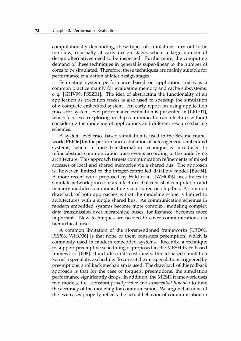
72 Chapter 3. Performance Evaluation
computationally demanding, these types of simulations turn out to betoo slow, especially at early design stages where a large number ofdesign alternatives need to be inspected. Furthermore, the computingdemand of these techniques in general is super-linear to the number ofcores to be simulated. Therefore, these techniques are mainly suitable forperformance evaluation at later design stages.
Estimating system performance based on application traces is acommon practice mainly for evaluating memory and cache subsystems,e. g. [GHV99, FSSZ01]. The idea of abstracting the functionality of anapplication as execution traces is also used to speedup the simulationof a complete embedded system. An early report on using applicationtraces for system-level performance estimation is presented in [LRD01],which focuses on exploring on-chip communication architectureswithoutconsidering the modeling of applications and different resource sharingschemes.
A system-level trace-based simulation is used in the Sesame frame-work [PEP06] for theperformance estimationofheterogeneous embeddedsystems, where a trace transformation technique is introduced torefine abstract communication trace events according to the underlyingarchitecture. This approach targets communication refinements of mixedaccesses of local and shared memories via a shared bus. The approachis, however, limited to the integer-controlled dataflow model [Buc94].A more recent work proposed by Wild et al. [WHO06] uses traces tosimulate network processor architectures that consist of computation andmemory modules communicating via a shared on-chip bus. A commondrawback of both approaches is that the modeling scope is limited toarchitectures with a single shared bus. As communication schemes inmodern embedded systems become more complex, modeling complexdata transmission over hierarchical buses, for instance, becomes moreimportant. New techniques are needed to cover communications viahierarchical buses.
A common limitation of the aforementioned frameworks [LRD01,PEP06, WHO06] is that none of them considers preemption, which iscommonly used in modern embedded systems. Recently, a techniqueto support preemptive scheduling is proposed in the MESH trace-basedframework [JP08]. It includes in its customized thread-based simulationkernel a speculative schedule. To correct themisspeculations triggered bypreemptions, a rollbackmechanism is used. Thedrawback of this rollbackapproach is that for the case of frequent preemptions, the simulationperformance significantly drops. In addition, the MESH framework usestwo models, i. e. , constant penalty value and exponential function to tunethe accuracy of the modeling for communication. We argue that none ofthe two cases properly reflects the actual behavior of communication in
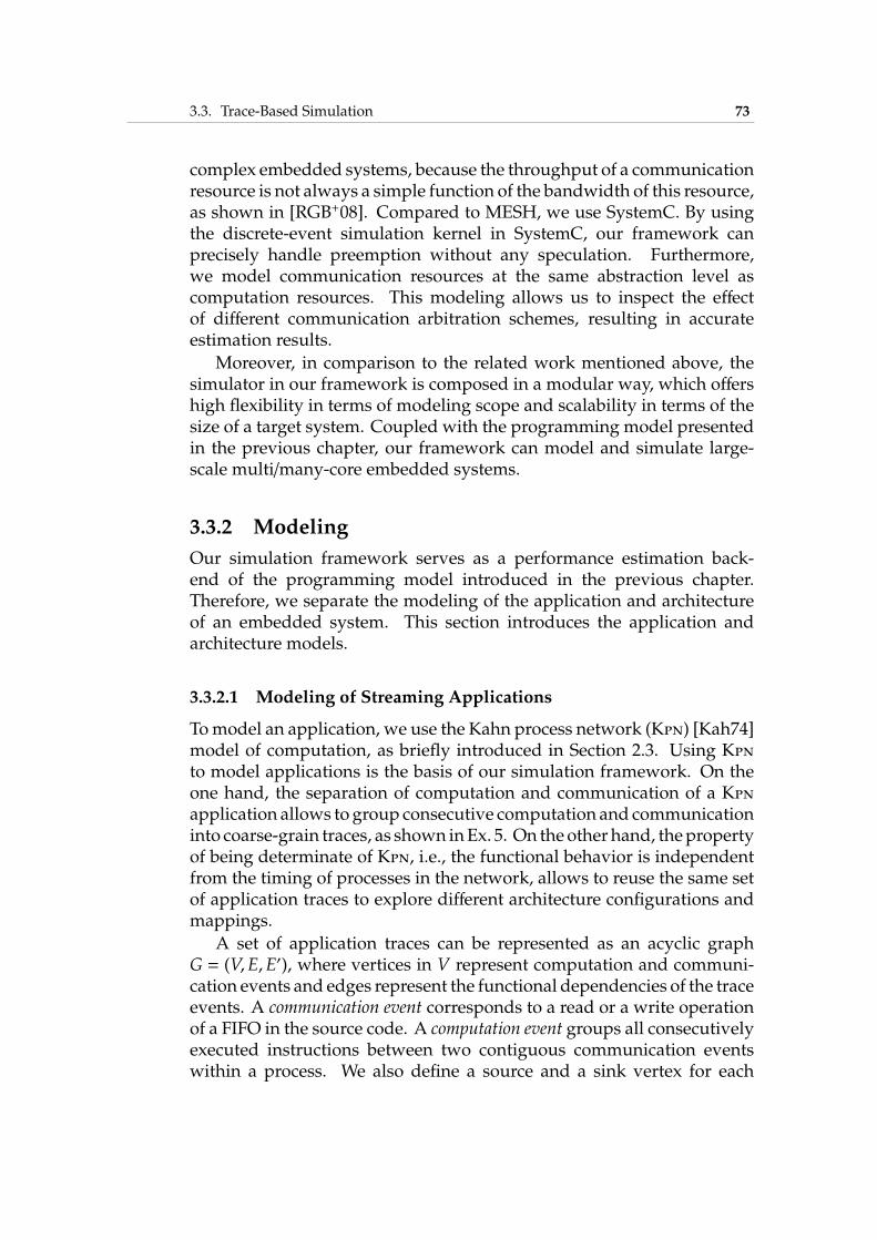
3.3. Trace-Based Simulation 73
complex embedded systems, because the throughput of a communicationresource is not always a simple function of the bandwidth of this resource,as shown in [RGB+08]. Compared to MESH, we use SystemC. By usingthe discrete-event simulation kernel in SystemC, our framework canprecisely handle preemption without any speculation. Furthermore,we model communication resources at the same abstraction level ascomputation resources. This modeling allows us to inspect the effectof different communication arbitration schemes, resulting in accurateestimation results.
Moreover, in comparison to the related work mentioned above, thesimulator in our framework is composed in a modular way, which offershigh flexibility in terms of modeling scope and scalability in terms of thesize of a target system. Coupled with the programming model presentedin the previous chapter, our framework can model and simulate large-scale multi/many-core embedded systems.
3.3.2 Modeling
Our simulation framework serves as a performance estimation back-end of the programming model introduced in the previous chapter.Therefore, we separate the modeling of the application and architectureof an embedded system. This section introduces the application andarchitecture models.
3.3.2.1 Modeling of Streaming Applications
Tomodel an application, we use the Kahn process network (Kpn) [Kah74]model of computation, as briefly introduced in Section 2.3. Using Kpnto model applications is the basis of our simulation framework. On theone hand, the separation of computation and communication of a Kpnapplication allows to group consecutive computation and communicationinto coarse-grain traces, as shown inEx. 5. On theother hand, thepropertyof being determinate of Kpn, i.e., the functional behavior is independentfrom the timing of processes in the network, allows to reuse the same setof application traces to explore different architecture configurations andmappings.
A set of application traces can be represented as an acyclic graphG = (V,E,E′), where vertices in V represent computation and communi-cation events and edges represent the functional dependencies of the traceevents. A communication event corresponds to a read or a write operationof a FIFO in the source code. A computation event groups all consecutivelyexecuted instructions between two contiguous communication eventswithin a process. We also define a source and a sink vertex for each
74 Chapter 3. Performance Evaluation
process to represent the starting and ending events for the traces of thisprocess. An edge in set E connects two consecutive events of a process,the direction of which specifies the functional order of these two events.An edge in set E′ connects inter-process communication events, i.e., awrite/read pair, corresponding to a data transmission via a Kpn FIFO.A graphical view of a set of application traces is shown in the followingexample.
Ex. 5: A process network consisting of three processes and the coarse-grained sourcecode of the processes are depicted in Fig. 42. The first iteration of the recurringpattern of the traces is shown in Fig. 43. A horizontal row in Fig. 43 representsa set of trace events for a process. The edges that connect two rows specify datadependencies between write/read pairs.
P1 P2 P3
C1
C2
C3
C4
P1.fire( ) {
P1_1.comp( );
C1.write( );
P1_2.comp( );
C2.read( );
}
P2.fire( ) {
C1.read( );
P2_1.comp( );
C3.write( );
C4.read( );
P2_2.comp( );
C2.write( );
}
p3.fire( ) {
P3_1.comp( );
C3.read( );
P3_2.comp( );
C4.write( );
}
Fig. 42: A process network with three processes and the coarse-grained source code of
processes.
In a set of application traces, the functionality of an application isabstracted as high-level trace events, whereas data dependencies betweenprocesses are captured as the ordering information between trace events.The trace sequence for a single process is totally ordered, i. e. , thechronological order of trace events is fixed. The edges in E′ impose apartial order on the trace events between different processes. The resultingacyclic partially ordered graph is fixed for a given input of the applicationand independent of any target architecture or mapping. This propertyallows to reuse the same partially ordered trace graph within the loop ofa design space exploration for inspecting differentmappings anddifferentarchitecture configurations.
To enable timing simulation, a computation event of a process isannotated with the runtime information of the corresponding code
3.3. Trace-Based Simulation 75
P1_1.comp C1.write P1_2.comp C2.read
C1.read P2_1.comp C3.write C4.read P2_2.comp C2.write
P3_1.comp C3.read P3_2.comp C4.write
Fig. 43: First iteration of the recurring pattern of the execution traces for the process
network in Fig. 42. Shadowed and black rectangles denote sources and sinks,
respectively.
segment for each processor to which the process can be mapped. We willexplain how to extract timing information of trace events in the follow-upsections. A communication event is annotated with the amount of datatransmitted from/to a FIFO. Note that a communication event will berefined to a set of new communication events during the simulation. Wedefine a basic unit by which a communication resource transmits data.During the simulation, a communication event will be split up into n newcommunication events, where n is the quotient between the amount ofdata in the original communication event and the basic unit.
3.3.2.2 Architecture modeling
One of our primary goals is to estimate the performance of embeddedsystems with multiple/many cores. In order to do so, we do notdifferentiate computation and communication resources in ourmodeling.We define virtual machines for timed processing of trace events andvirtual paths for the routing of communicated data. Based on thisscheme, an architecture for a target system can be easily composed. Bysimply varying the interconnects as well as scheduling policies of virtualmachines, different design alternatives can be quickly inspected, at anabstract level.
Virtual Machine
A virtual machine (VM) is defined as an autonomous unit, simulatingthe timing behavior of a computation and communication resource. Wemodel a VM as a 2-tuple V = (S,C), where S represents a schedulerand C is the capability, e.g. bus bandwidth or core frequency. Thescheduler S manages the mutual exclusive processing of multiple inputevent queues and C decides how time advances. For a computation
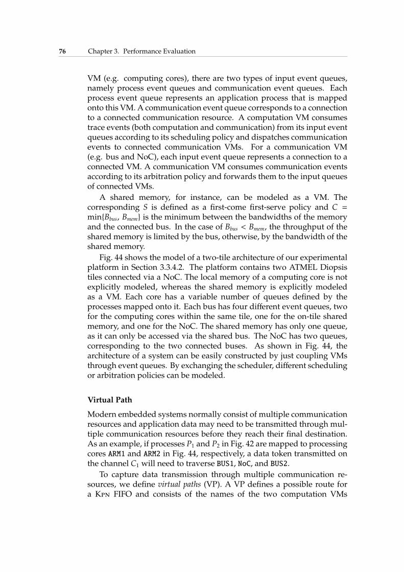
76 Chapter 3. Performance Evaluation
VM (e.g. computing cores), there are two types of input event queues,namely process event queues and communication event queues. Eachprocess event queue represents an application process that is mappedonto this VM. A communication event queue corresponds to a connectionto a connected communication resource. A computation VM consumestrace events (both computation and communication) from its input eventqueues according to its scheduling policy and dispatches communicationevents to connected communication VMs. For a communication VM(e.g. bus and NoC), each input event queue represents a connection to aconnected VM. A communication VM consumes communication eventsaccording to its arbitration policy and forwards them to the input queuesof connected VMs.
A shared memory, for instance, can be modeled as a VM. Thecorresponding S is defined as a first-come first-serve policy and C =min{Bbus, Bmem} is the minimum between the bandwidths of the memoryand the connected bus. In the case of Bbus < Bmem, the throughput of theshared memory is limited by the bus, otherwise, by the bandwidth of theshared memory.
Fig. 44 shows the model of a two-tile architecture of our experimentalplatform in Section 3.3.4.2. The platform contains two ATMEL Diopsistiles connected via a NoC. The local memory of a computing core is notexplicitly modeled, whereas the shared memory is explicitly modeledas a VM. Each core has a variable number of queues defined by theprocesses mapped onto it. Each bus has four different event queues, twofor the computing cores within the same tile, one for the on-tile sharedmemory, and one for the NoC. The shared memory has only one queue,as it can only be accessed via the shared bus. The NoC has two queues,corresponding to the two connected buses. As shown in Fig. 44, thearchitecture of a system can be easily constructed by just coupling VMsthrough event queues. By exchanging the scheduler, different schedulingor arbitration policies can be modeled.
Virtual Path
Modern embedded systems normally consist of multiple communicationresources and application data may need to be transmitted through mul-tiple communication resources before they reach their final destination.As an example, if processes P1 and P2 in Fig. 42 are mapped to processingcores ARM1 and ARM2 in Fig. 44, respectively, a data token transmitted onthe channel C1 will need to traverse BUS1, NoC, and BUS2.
To capture data transmission through multiple communication re-sources, we define virtual paths (VP). A VP defines a possible route fora Kpn FIFO and consists of the names of the two computation VMs
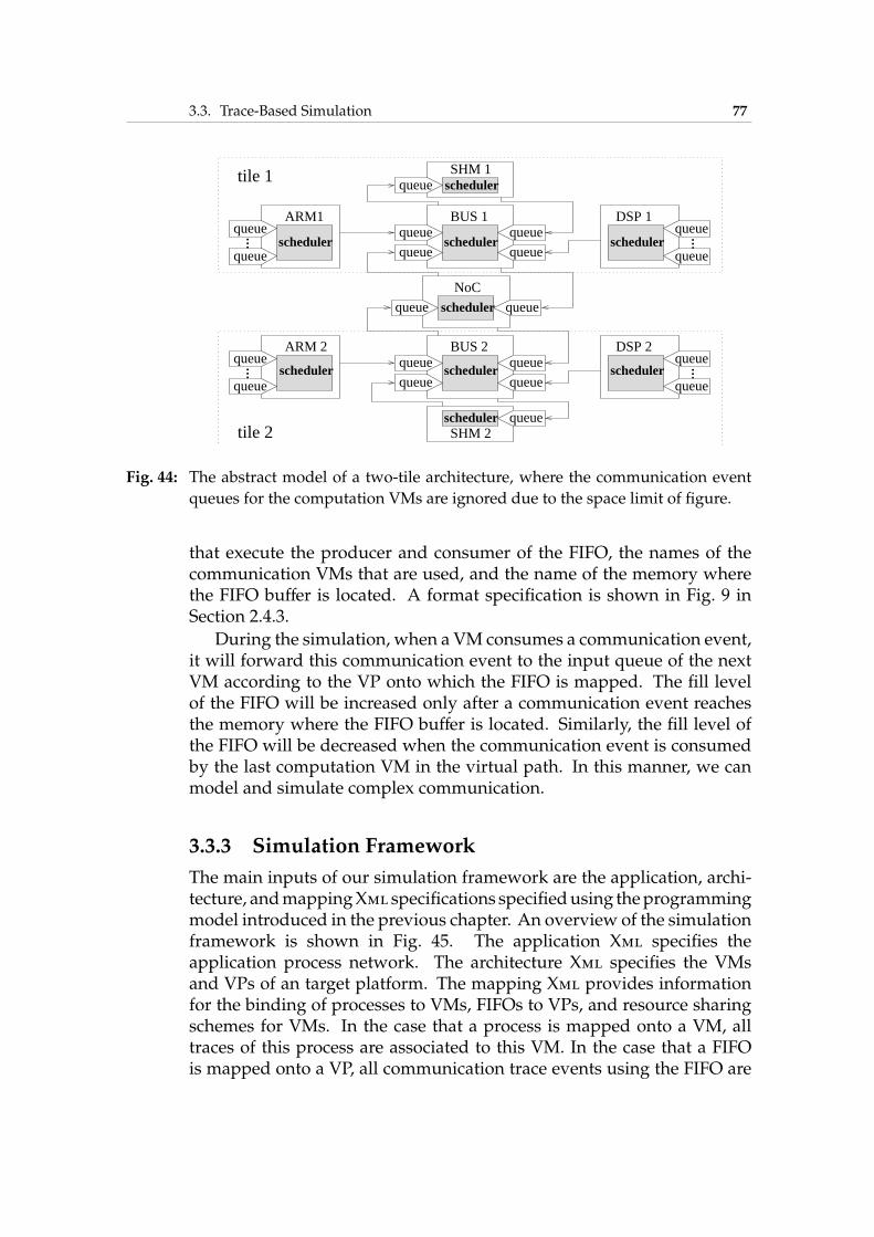
3.3. Trace-Based Simulation 77
...
...
...
...
NoC
DSP 2BUS 2ARM 2
ARM1
SHM 1
BUS 1 DSP 1
scheduler
scheduler
SHM 2scheduler
scheduler
schedulerscheduler
schedulerscheduler scheduler
queue
tile 2
queue
queue
queue
queue queue
queue
queue
queue
queue
queue queue
queue
queue
queue
queue
queue
tile 1
queue
queue
queue
Fig. 44: The abstract model of a two-tile architecture, where the communication event
queues for the computation VMs are ignored due to the space limit of figure.
that execute the producer and consumer of the FIFO, the names of thecommunication VMs that are used, and the name of the memory wherethe FIFO buffer is located. A format specification is shown in Fig. 9 inSection 2.4.3.
During the simulation, when a VM consumes a communication event,it will forward this communication event to the input queue of the nextVM according to the VP onto which the FIFO is mapped. The fill levelof the FIFO will be increased only after a communication event reachesthe memory where the FIFO buffer is located. Similarly, the fill level ofthe FIFO will be decreased when the communication event is consumedby the last computation VM in the virtual path. In this manner, we canmodel and simulate complex communication.
3.3.3 Simulation Framework
The main inputs of our simulation framework are the application, archi-tecture, andmappingXml specifications specifiedusing theprogrammingmodel introduced in the previous chapter. An overview of the simulationframework is shown in Fig. 45. The application Xml specifies theapplication process network. The architecture Xml specifies the VMsand VPs of an target platform. The mapping Xml provides informationfor the binding of processes to VMs, FIFOs to VPs, and resource sharingschemes for VMs. In the case that a process is mapped onto a VM, alltraces of this process are associated to this VM. In the case that a FIFOis mapped onto a VP, all communication trace events using the FIFO are
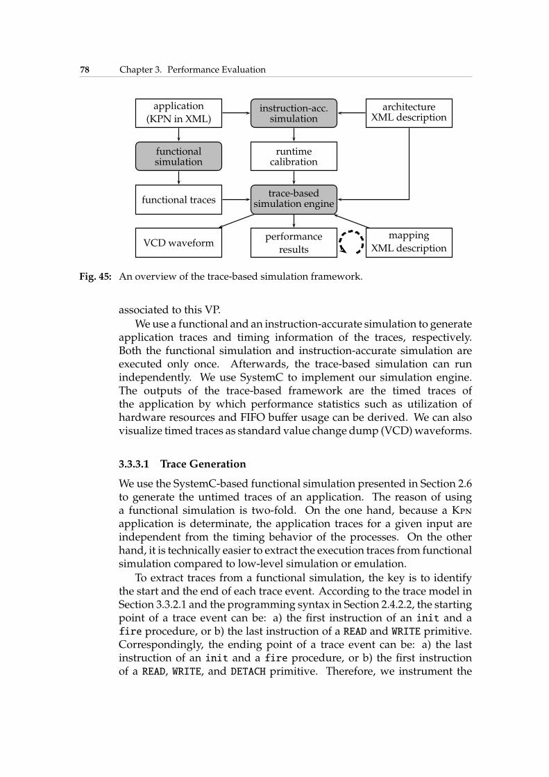
78 Chapter 3. Performance Evaluation
application
(KPN in XML)instruction-acc.
simulationarchitecture
XML description
functionalsimulation
runtimecalibration
functional tracestrace-based
simulation engine
VCD waveformperformance
results
mapping
XML description
Fig. 45: An overview of the trace-based simulation framework.
associated to this VP.
We use a functional and an instruction-accurate simulation to generateapplication traces and timing information of the traces, respectively.Both the functional simulation and instruction-accurate simulation areexecuted only once. Afterwards, the trace-based simulation can runindependently. We use SystemC to implement our simulation engine.The outputs of the trace-based framework are the timed traces ofthe application by which performance statistics such as utilization ofhardware resources and FIFO buffer usage can be derived. We can alsovisualize timed traces as standard value change dump (VCD)waveforms.
3.3.3.1 Trace Generation
We use the SystemC-based functional simulation presented in Section 2.6to generate the untimed traces of an application. The reason of usinga functional simulation is two-fold. On the one hand, because a Kpnapplication is determinate, the application traces for a given input areindependent from the timing behavior of the processes. On the otherhand, it is technically easier to extract the execution traces from functionalsimulation compared to low-level simulation or emulation.
To extract traces from a functional simulation, the key is to identifythe start and the end of each trace event. According to the trace model inSection 3.3.2.1 and the programming syntax in Section 2.4.2.2, the startingpoint of a trace event can be: a) the first instruction of an init and afire procedure, or b) the last instruction of a READ and WRITE primitive.Correspondingly, the ending point of a trace event can be: a) the lastinstruction of an init and a fire procedure, or b) the first instructionof a READ, WRITE, and DETACH primitive. Therefore, we instrument the
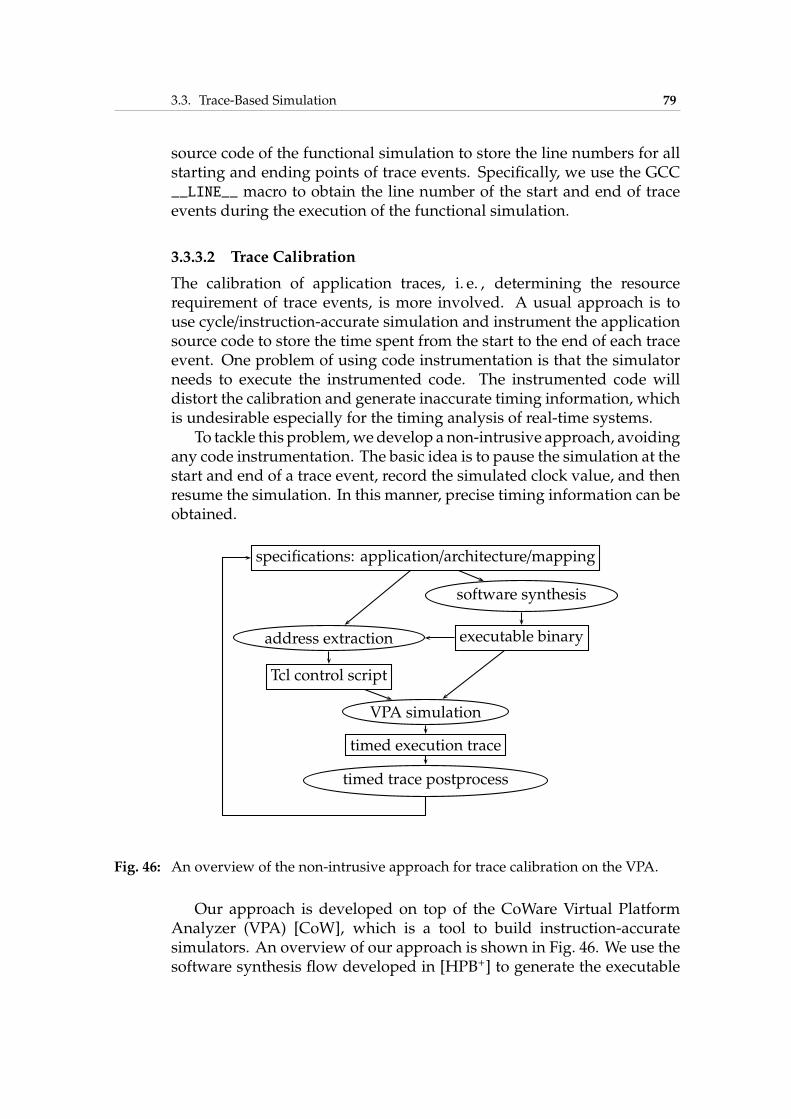
3.3. Trace-Based Simulation 79
source code of the functional simulation to store the line numbers for allstarting and ending points of trace events. Specifically, we use the GCC__LINE__ macro to obtain the line number of the start and end of traceevents during the execution of the functional simulation.
3.3.3.2 Trace Calibration
The calibration of application traces, i. e. , determining the resourcerequirement of trace events, is more involved. A usual approach is touse cycle/instruction-accurate simulation and instrument the applicationsource code to store the time spent from the start to the end of each traceevent. One problem of using code instrumentation is that the simulatorneeds to execute the instrumented code. The instrumented code willdistort the calibration and generate inaccurate timing information, whichis undesirable especially for the timing analysis of real-time systems.
To tackle this problem,wedevelop a non-intrusive approach, avoidingany code instrumentation. The basic idea is to pause the simulation at thestart and end of a trace event, record the simulated clock value, and thenresume the simulation. In this manner, precise timing information can beobtained.
specifications: application/architecture/mapping
software synthesis
address extraction executable binary
Tcl control script
VPA simulation
timed execution trace
timed trace postprocess
Fig. 46: An overview of the non-intrusive approach for trace calibration on the VPA.
Our approach is developed on top of the CoWare Virtual PlatformAnalyzer (VPA) [CoW], which is a tool to build instruction-accuratesimulators. An overview of our approach is shown in Fig. 46. We use thesoftware synthesis flow developed in [HPB+] to generate the executable
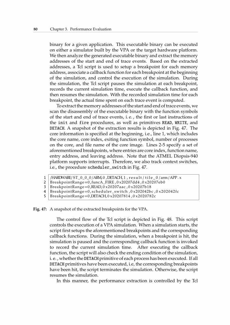
80 Chapter 3. Performance Evaluation
binary for a given application. This executable binary can be executedon either a simulator built by the VPA or the target hardware platform.We then analyze the generated executable binary and extract the memoryaddresses of the start and end of trace events. Based on the extractedaddresses, a Tcl script is used to setup a breakpoint for each memoryaddress, associate a callback function for each breakpoint at the beginningof the simulation, and control the execution of the simulation. Duringthe simulation, the Tcl script pauses the simulation at each breakpoint,records the current simulation time, execute the callback function, andthen resumes the simulation. With the recorded simulation time for eachbreakpoint, the actual time spent on each trace event is computed.
To extract thememoryaddresses of the start andendof trace events,wescan the disassembly of the executable binary with the function symbolsof the start and end of trace events, i. e. , the first or last instructions ofthe init and fire procedures, as well as primitives READ, WRITE, andDETACH. A snapshot of the extraction results is depicted in Fig. 47. Thecore information is specified at the beginning, i.e., line 1, which includesthe core name, core index, exiting function symbol, number of processeson the core, and file name of the core image. Lines 2-5 specify a set ofaforementioned breakpoints, where entries are core index, function name,entry address, and leaving address. Note that the ATMEL Diopsis-940platform supports interrupts. Therefore, we also track context switches,i.e., the procedure scheduler_switch in Fig. 47.
1 /HARDWARE/ ST_0_0_0 /ARM, 0 ,DETACH, 1 , r e su l t / t i l e _ 0 / arm /APP. x2 BreakpointRange=0 , funcA_FIRE , 0 x20207dd4 , 0 x20207eb03 BreakpointRange=0 ,READ, 0 x20207aac , 0 x20207b184 BreakpointRange=0 , scheduler_switch , 0 x202042bc , 0 x202042fc5 BreakpointRange=0 ,DETACH,0 x20207814 , 0 x2020782c
Fig. 47: A snapshot of the extracted breakpoints for the VPA.
The control flow of the Tcl script is depicted in Fig. 48. This scriptcontrols the execution of a VPA simulation. When a simulation starts, thescript first setups the aforementioned breakpoints and the correspondingcallback functions. During the simulation, when a breakpoint is hit, thesimulation is paused and the corresponding callback function is invokedto record the current simulation time. After executing the callbackfunction, the script will also check the ending condition of the simulation,i. e. , whether the DETACHprimitive of eachprocess has been executed. If allDETACH primitives have been executed, i.e, the corresponding breakpointshave been hit, the script terminates the simulation. Otherwise, the scriptresumes the simulation.
In this manner, the performance extraction is controlled by the Tcl
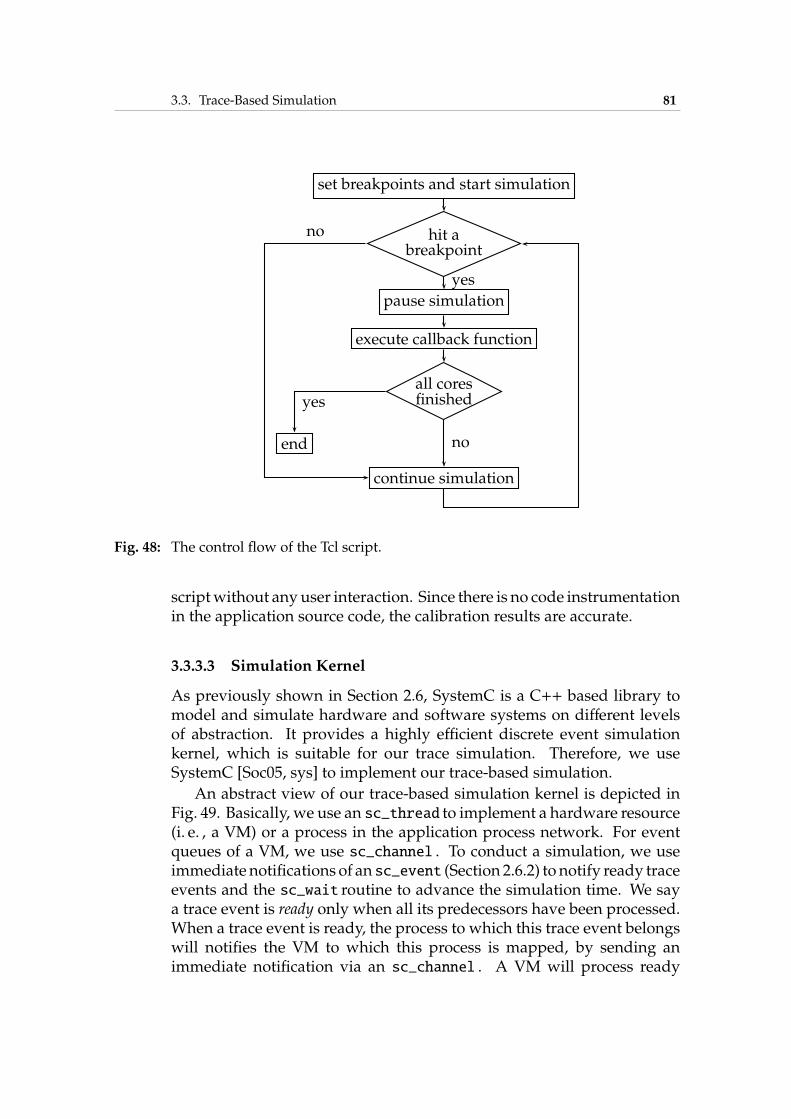
3.3. Trace-Based Simulation 81
set breakpoints and start simulation
hit abreakpoint
pause simulation
execute callback function
all coresfinished
end
continue simulation
no
yes
no
yes
Fig. 48: The control flow of the Tcl script.
scriptwithout anyuser interaction. Since there is no code instrumentationin the application source code, the calibration results are accurate.
3.3.3.3 Simulation Kernel
As previously shown in Section 2.6, SystemC is a C++ based library tomodel and simulate hardware and software systems on different levelsof abstraction. It provides a highly efficient discrete event simulationkernel, which is suitable for our trace simulation. Therefore, we useSystemC [Soc05, sys] to implement our trace-based simulation.
An abstract view of our trace-based simulation kernel is depicted inFig. 49. Basically, we use an sc_thread to implement a hardware resource(i. e. , a VM) or a process in the application process network. For eventqueues of a VM, we use sc_channel . To conduct a simulation, we useimmediate notifications of an sc_event (Section 2.6.2) to notify ready traceevents and the sc_wait routine to advance the simulation time. We saya trace event is ready only when all its predecessors have been processed.When a trace event is ready, the process to which this trace event belongswill notifies the VM to which this process is mapped, by sending animmediate notification via an sc_channel . A VM will process ready
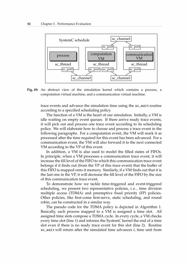
82 Chapter 3. Performance Evaluation
SystemC schedule
sc_channel sc_channel
sc_channel
sc_port sc_port sc_port sc_port
sc_port sc_port
sc_thread
process
sc_thread
computationVM
sc_thread
communicationVM
Fig. 49: An abstract view of the simulation kernel which contains a process, a
computation virtual machine, and a communication virtual machine.
trace events and advance the simulation time using the sc_wait routineaccording to a specified scheduling policy.
The function of a VM is the heart of our simulation. Initially, a VM isidle waiting on empty event queues. If there arrive ready trace events,it will pick out and process one trace event according to its schedulingpolice. We will elaborate how to choose and process a trace event in thefollowing paragraphs. For a computation event, the VM will mark it asprocessed after the time required for this event has been advanced. For acommunication event, the VM will also forward it to the next connectedVM according to the VP of this event.
In addition, a VM is also used to model the filled states of FIFOs.In principle, when a VM processes a communication trace event, it willincrease the fill level of the FIFO to which this communication trace eventbelongs if it finds out (from the VP of this trace event) that the buffer ofthis FIFO is mapped onto it memory. Similarly, if a VM finds out that it isthe last one in the VP, it will decrease the fill level of the FIFO by the sizeof this communication trace event.
To demonstrate how we tackle time-triggered and event-triggeredscheduling, we present two representative policies, i. e. , time divisionmultiple access (TDMA) and preemptive fixed priority (FP) policies.Other policies, like first-come first-serve, static scheduling, and roundrobin, can be constructed in a similar way.
The pseudo code for the TDMA policy is depicted in Algorithm 1.Basically, each process mapped to a VM is assigned a time slot. Allassigned time slots compose a TDMA cycle. In every cycle, a VM checksevery time slot (line 1) and informs the SystemC kernel the end of a timeslot even if there is no ready trace event for this slot (line 2). Routinesc_waitwill return after the simulated time advances ti time unit from
3.3. Trace-Based Simulation 83
the current simulated time. After time for a time slot is advanced, readytrace events that belong to this time slot are processed (line 3). If a traceevent cannot finish at currently slot, the unprocessed part of it will haveto wait for its slot in the next cycle, see line 5-6.
Algorithm 1 TDMA scheduling of a virtual machineV
1: for each slot i do2: sc_wait(ti) ⊲ ti is length of slot i3: while ∃ ei, j ∈ slot i∨ ti > 0 do ⊲ There is a ready event ei, j for slot i4: if tei, j > ti then ⊲ Required time longer than the length of slot i5: tei, j ← tei, j − ti6: ti ← 07: else8: ti ← ti − tei, j9: j + + ⊲ ei, j is processed. Can continue to the next ready
event10: end if11: end while12: end for
The pseudo code for the FP scheduling is depicted in Algorithm 2. Itworks differently in comparison to the TDMA scheduling. Only whenthere is a ready trace event, the scheduler will inform the SystemCkernel how much time it needs in order to process this trace event,as shown in line 3. Besides the timeout tei, j , the routine sc_waitwillregister an sc_event that serves as an interrupt event. If a trace event of ahigher priority process comes before the timeout tei, j , the interrupt eventIRQ_event will be activated and routine sc_waitwill return with theactual advanced time, as shown in line 5–7. The scheduler will continuewith the new highest priority trace event.
Algorithm 2 FP scheduling of a virtual machineV
1: while ∃ ei, j do ⊲ Get the highest ready event from all queues2: told ← sc_simulation_time( )3: sc_wait(tei, j , IRQ_event) ⊲ Interrupt event IRQ_event4: tnew ← sc_simulation_time( )5: if tnew − told < tei, j then ⊲ The actual advanced time6: tei, j ← tei, j − (tnew − told)7: end if8: end while
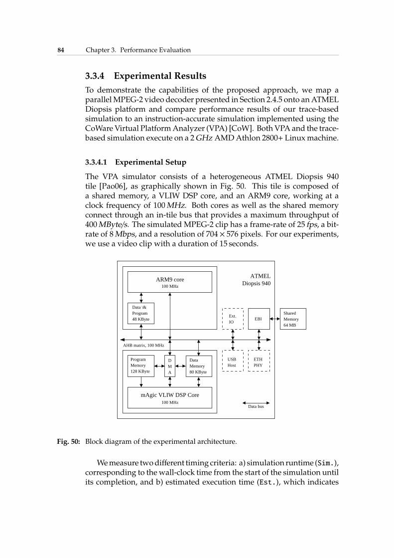
84 Chapter 3. Performance Evaluation
3.3.4 Experimental Results
To demonstrate the capabilities of the proposed approach, we map aparallelMPEG-2 video decoder presented in Section 2.4.5 onto anATMELDiopsis platform and compare performance results of our trace-basedsimulation to an instruction-accurate simulation implemented using theCoWare Virtual PlatformAnalyzer (VPA) [CoW]. BothVPA and the trace-based simulation execute on a 2GHz AMDAthlon 2800+ Linuxmachine.
3.3.4.1 Experimental Setup
The VPA simulator consists of a heterogeneous ATMEL Diopsis 940tile [Pao06], as graphically shown in Fig. 50. This tile is composed ofa shared memory, a VLIW DSP core, and an ARM9 core, working at aclock frequency of 100MHz. Both cores as well as the shared memoryconnect through an in-tile bus that provides a maximum throughput of400MByte/s. The simulated MPEG-2 clip has a frame-rate of 25 fps, a bit-rate of 8Mbps, and a resolution of 704 × 576 pixels. For our experiments,we use a video clip with a duration of 15 seconds.
Memory80 KByte
DataMemory128 KByte
Program
MD
A
Data \&Program48 KByte
USBHost PHY
ETH
Ext.IO
SharedMemory64 MB
ARM9 core
mAgic VLIW DSP Core100 MHz
AHB matrix, 100 MHz
EBI
Data bus
100 MHz
ATMELDiopsis 940
Fig. 50: Block diagram of the experimental architecture.
Wemeasure twodifferent timing criteria: a) simulation runtime (Sim.),corresponding to the wall-clock time from the start of the simulation untilits completion, and b) estimated execution time (Est.), which indicates
3.3. Trace-Based Simulation 85
how long the decoder needs to finish the decoding of the 15 second video.All time values are rounded to seconds.
3.3.4.2 Experimental Results
For the first experiment, we map a pipelined version of MPEG-2 decoder(shown in Fig. 11(a) in Section 2.4.5) onto a single Diopsis 940 tile. Weinvestigate three different mappings. Mapping 1 uses only the ARM coreof a tile, i.e., all processes are mapped onto an ARM core and all FIFObuffers are located in the local memory of the ARM core. Mapping 2uses the same process mapping as in Mapping 1whereas FIFO buffers aremapped to the shared memory. Mapping 3 maps the most computationintensive process, i.e., transform_block, onto the DSP core and thebuffers for those FIFOs connecting to transform_block are set to theshared memory.
CaseEst. time (hh:mm:ss) Sim. time (hh:mm:ss)TSim VPA Error TSim VPA Speedup
1 1:36:51 1:38:26 -3% 0:03:28 30:34:00 6112 1:54:13 1:52:20 +2% 0:03:30 31:30:00 6303 0:17:17 0:16:46 +3% 0:03:30 74:19:00 1466
Tab. 5: Estimated execution time and simulation time for the considered mappings,
when decoding a 15 s MPEG-2 video.
The experimental results are presented in Tab. 5. From the table, wecan find out that our trace-based simulation obtains a high accuracy forall three mappings. The error rate in comparison to the VPA instruction-accurate simulation iswithin 3%. Thedeviation ismainly due to the cacheeffect in the platform, which is currently not modeled in our trace-basedsimulation. In terms of simulation speed, our trace-based simulation isconsiderably faster than the VPA simulation. We obtain two and threeorders of magnitude speedup for the single core and dual cores cases,respectively. The reason is that our simulation does not execute theapplication, which is computationally expensive. In addition, a hardwareresource in our model, i.e., a virtual machine, works only as a traceevent dispatcher and does not simulate instruction-level behavior, whichfurther reduces the simulation runtime.
In the second experiment, we simulate Mapping 1with different sizesof the FIFOs in the process network. The simulation results are shown inTab. 6. From the table, we can find out that the error rate is again about3%. Note that the Est. time for MPEG-2 decode increases as the size of
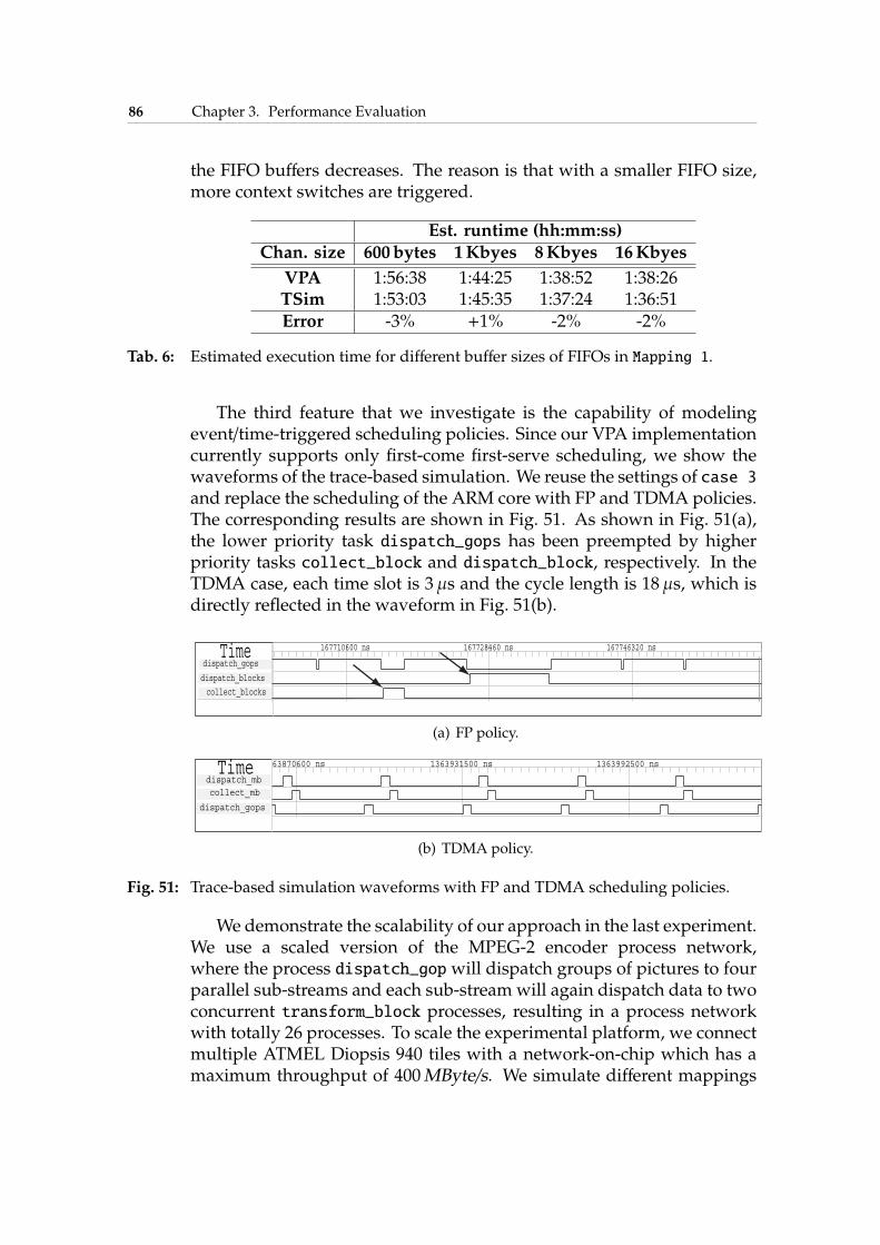
86 Chapter 3. Performance Evaluation
the FIFO buffers decreases. The reason is that with a smaller FIFO size,more context switches are triggered.
Est. runtime (hh:mm:ss)
Chan. size 600 bytes 1Kbyes 8Kbyes 16Kbyes
VPA 1:56:38 1:44:25 1:38:52 1:38:26TSim 1:53:03 1:45:35 1:37:24 1:36:51Error -3% +1% -2% -2%
Tab. 6: Estimated execution time for different buffer sizes of FIFOs in Mapping 1.
The third feature that we investigate is the capability of modelingevent/time-triggered scheduling policies. Since our VPA implementationcurrently supports only first-come first-serve scheduling, we show thewaveforms of the trace-based simulation. We reuse the settings of case 3and replace the scheduling of the ARM core with FP and TDMA policies.The corresponding results are shown in Fig. 51. As shown in Fig. 51(a),the lower priority task dispatch_gops has been preempted by higherpriority tasks collect_block and dispatch_block, respectively. In theTDMA case, each time slot is 3µs and the cycle length is 18µs, which isdirectly reflected in the waveform in Fig. 51(b).
(a) FP policy.
(b) TDMA policy.
Fig. 51: Trace-based simulation waveforms with FP and TDMA scheduling policies.
We demonstrate the scalability of our approach in the last experiment.We use a scaled version of the MPEG-2 encoder process network,where the process dispatch_gop will dispatch groups of pictures to fourparallel sub-streams and each sub-stream will again dispatch data to twoconcurrent transform_block processes, resulting in a process networkwith totally 26 processes. To scale the experimental platform, we connectmultiple ATMEL Diopsis 940 tiles with a network-on-chip which has amaximum throughput of 400MByte/s. We simulate different mappings
3.4. Summary 87
with up to eight tiles. The simulation time is shown in Tab. 7. Thesimulation time of our simulations increases only by 18%, even wheneight times more hardware resources are simulated. The reason for theincrement of the simulation time is that with more tiles added, morecommunication trace events need to be transmitted through multiplecommunication media. These multi-hop communication trace eventsconsume additional simulation time.
TilesSimulation time
(hh:mm:ss)
1 0:05:082 0:05:294 0:05:438 0:06:04
Tab. 7: Simulation time for 1, 2, 4, 8 tiles.
3.4 Summary
In this chapter, we investigate techniques to estimate the timing behaviorof streaming embedded systems. We describe two different methods, i.e.,a formal analytic method and a simulation-based technique.
For the analytic approach,we inspect timing correlations betweendatastreams and present a newmethod to analyze correlated data streams thatoriginate from the same source. By means of the proposed method, wecan obtain considerably tighter performance bounds than those usingprevious methods. We show the applicability of the presented methodby analyzing a concrete multimedia application. Although this methodis implemented within the Rtc-mpa framework, the idea behind can alsobe applied to other modular analysis frameworks, such as SymTA/S.
For the simulation-based approach, we propose a trace-based frame-work, which can simulate the timing behavior of complex multi/many-core embedded systems. By abstracting application functionalityinto coarse-grained traces and simulating a system at system level,our simulation is orders of magnitude faster than instruction-accuratesimulations. On the other hand, by capturing essential system properties,e. g. scheduling andbuffer location, togetherwith the intrinsic characteris-tics of streaming system, e. g. stable pipelined stage and small cache effect,we obtain high accuracy compared to instruction-accurate simulations.
Another advantage of our techniques is that both the analytic methodand the trace-based simulation can serve as a non-functional back-end for

88 Chapter 3. Performance Evaluation
the programmingmodel defined in the previous chapter. Both techniquescan thereby be embedded into an automated design space exploration toassist the software design of embedded systems.
In the next chapter, we will inspect another design metric, i.e., thepower metric. In particular, we investigate system-level power-efficientdesign under certain performance constraints.
4Power Management
Power dissipation has been an important design issue in a wide range ofcomputer systems in the past decades. Power management with energyefficiency considerations is helpful for server systems to reduce powerbills. Efficient power management is even more crucial for embeddedsystems. A major category of embedded systems, for instance, arehand-held mobile devices that are powered by batteries. The batteriesfor such devices are limited in both power and energy output. Theamount of energy available thus severely limits a system’s lifespan.Although research continues to develop batteries with higher energy-density, the slow growth of the energy density of batteries lags far behindthe tremendous increase of demands [ITR]. Because of these facts, powerconsumption becomes one of the first-class design concerns for moderncomputer systems, in particular for multi-core and future many-coreembedded systems.
Two major sources of power consumption of a CMOS circuit aredynamic power consumption due to transistor switching activitiesand static power consumption due to leakage current [JPG04]. Formicrometer-scale semiconductor technology, dynamic power dominatesthe power consumption of a processor. However, as modern VLSItechnology is scaling down to the deep sub-micron domain, chipsconsume significantly more static power. The leakage current thatoriginates from the dramatic increase in both sub-threshold currentand gate-oxide leakage current is projected to account for as much as50% of the total power dissipation for high-end processors in 90nmtechnologies [ABM+04]. The International Technology Road-map for
90 Chapter 4. Power Management
Semiconductors (ITRS) expects that the percentage of static power ofthe total power dissipation in the future will be much greater due tovariability and temperature effects [ITR].
On the other hand, the increasing number of integrated cores of anembedded platform provides opportunities to efficiently harness thestatic power consumption, e.g., switching those idle cores to a sleepmode to reduce leakage current. An interesting research question ishow to schedule the mode switches of those idle cores under real-timerequirements.
4.1 Overview
In the previous chapter, we investigated the performance metric ofmulti/many-core embedded systems and presented techniques forsystem-level performance estimation. This chapter studies anothermetric, i. e. , power metric. We focus on streaming embedded systemsat system level and study efficient power management under certainperformance constraints. Specifically, we make use of the worst-caseanalysis method, i.e., real-time calculus and explore how to applydynamic power management to reduce static power consumption whilesatisfying real-time constraints.
For simplicity, we consider a dual-core scenario, i.e., a processingcore for data stream processing and a control core for coordination, e.g.,scheduling. The processing core has three power modes, i.e., active,standby, and sleep modes, with different power consumptions. Thecontrol core decides when to change the power modes of the processingcore. Intuitively, the processing core can be switched off to sleep modeto reduce the power consumption when it becomes idle and switchedto active mode again upon the arrival of an event. These switchingoperations, however, need more careful consideration. On the one hand,the sleep period of the processing core after switching-off should be longenough to recuperate mode-switch overheads. On the other hand, whento activate the processing core is even more involved due to the possibleburstiness of future event arrivals. For every switching-on operation,sufficient time has to be reserved to serve the possible burstiness of futureevents in order to prevent deadline violation of events or overflow ofsystem backlog.
To resolve these concerns, we propose both online and offlinealgorithms that are applicable particularly for embedded systems.We apply real-time calculus to predict future event arrival and real-time interface theory [TWS06] for schedulability analysis, trying toprocrastinate the buffered and future events as late as possible. Our offline
4.2. Related Work 91
algorithms compute optimal and approximate schemes for periodicpower management. Alternatively, our online algorithms adaptivelypredict the next mode-switch moment by considering both past andfuture event arrivals. Based on the adopted worst-case interval-basedabstraction, our algorithms can not only tackle arbitrary event arrivals,e.g., with burstiness, but also guarantee hard real-time constraints withrespect to both timing and backlog constraints. To handle multiple eventstreams, we propose solutions for two preemptive scheduling policies,i.e., earliest-deadline-first and fixed priority. Although our algorithms aredeveloped for a dual-core scenario, the principle behind can be applied tomulti/many-core platforms, in particular the class of platforms using tile-based architectures, e. g. , Intel SCC [SCC] and ATMEL ShapOtto [HPB+].
The rest of this chapter is organized as follows: The next sectionreviews the related work in the literature. Section 4.3 provides systemmodels. Section 4.4 presents a set of new routines which will beused throughout this chapter. Section 4.5 presents our proposed onlinealgorithms for one event stream, while Section 4.6 copes with multipleevent streams. The offline periodic power management approach ispresented in Section 4.7. Simulations results are presented within eachsection and Section 4.8 summarizes the chapter.
4.2 Related Work
Power estimation techniques are important for energy-efficient em-bedded system designs. To estimate the power consumption of amicroprocessor at abstract level, analytic methods [BFSS00, MPS98]based on statistical or information-theoretic techniques and simulation-based approaches [BTM00, YVKI00] based on instruction set simulators(ISSs) are widely used. To leverage the trade-off between accuracy andestimation speed, trace-based power simulation [vSP10] is also proposedto evaluate the power consumption of a system.
To analyze power-aware real-time behavior of an embedded system,event-stream based models are commonly adopted. Baptiste [Bap06]proposes an algorithm based on dynamic programming to control whento turn on/off a device for aperiodic real-time events with the sameexecution time. For multiple low-power modes, Augustine et al. [AIS04]determine the mode that a processor should enter for aperiodic real-timeevents and propose a competitive algorithm for online use. Swaminathanet al. [SC05] explore dynamic power management and develop offlinealgorithms to find the exact starting time of real-time events and tocompute an approximation in polynomial time. To aggregate the idle timefor energy reduction, Shrivastava et al. [SEDN05] propose a framework
92 Chapter 4. Power Management
for code transformations. By considering platforms with both DPM anddynamic voltage scaling (DVS), Chen and Kuo [CK07] propose to executetasks at a certain speed and to control the procrastination of real-timeevents. By turning the device to the sleep mode, the execution of theprocrastinated real-time events is aggregated in a busy interval to reduceenergy consumption. Heo [HHLA07] et al. explore how to integratedifferent power management policies in a server farm. Alternatively,Devadas and Aydin [DA08, DA10] consider the interplay between DVSandDPMona systemwith aDVS-capable processor andmultiple devices.Basedon the concept of forbidden regions, the authorspropose algorithmsto determine the optimal processor speed as well as transition decisionsof device states to minimize overall system energy for periodic real-timetasks.
Most of the above approaches require either precise information ofevent arrivals, such as periodic real-time events [CK07], or aperiodic real-time events with known arrival time [Bap06, AIS04, ISG03]. We arguethat the abstraction is, however, too coarse. In practice, the precise timinginformation of event arrivals might not be known in advance since thearrival time depends on many factors. When the precise timing of eventarrivals is unknown, to our best knowledge, the only known approachesare to apply the online algorithms proposed by Irani et al. [ISG03] andAugustine et al. [AIS04] to control when to turn on the device. However,since the online algorithms in [AIS04, ISG03] greedily stay in the sleepmode as long as possible without referring to incoming events in the nearfuture, the resulting schedule might make an event miss its deadline.Such algorithms are not applicable for hard real-time systems.
Tomodel irregular arrival patterns of event streams, real-time calculus,based on Network Calculus [Cru91b], was proposed by Thiele et al.[TCN00, WTVL06] to characterize events with arrival curves. The arrivalcurve of an event stream describes the upper and lower bounds of thenumber of events arriving at the system for a specified interval. Therefore,schedulability analysis can be done based on the arrival curves of eventstreams. In [MCT05], Maxiaguine et al. apply real-time calculus withinthe DVS context and compute a safe frequency at periodical intervalswith predefined length to prevent buffer overflow of a system. Chenet al. [CST09] explore the schedulability for on-line DVS schedulingalgorithms when the event arrivals are constrained by a given upperarrival curve. In contrast to these closely related approaches, we focuson dynamic power management. We propose offline algorithms to findperiodic time-driven patterns to turn on/off devices for energy savingswithout sacrificing timing guarantees. The small run-time overhead ofthe periodic schemes is very suitable for embedded systems that onlyhave limited computational power. We also propose online algorithms
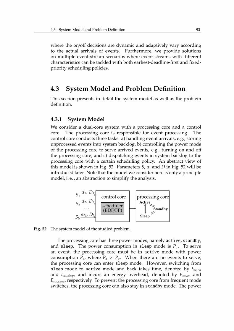
4.3. System Model and Problem Definition 93
where the on/off decisions are dynamic and adaptively vary accordingto the actual arrivals of events. Furthermore, we provide solutionson multiple event-stream scenarios where event streams with differentcharacteristics can be tackled with both earliest-deadline-first and fixed-priority scheduling policies.
4.3 System Model and Problem Definition
This section presents in detail the system model as well as the problemdefinition.
4.3.1 System Model
We consider a dual-core system with a processing core and a controlcore. The processing core is responsible for event processing. Thecontrol core conducts three tasks: a) handling event arrivals, e.g., storingunprocessed events into system backlog, b) controlling the power modeof the processing core to serve arrived events, e.g., turning on and offthe processing core, and c) dispatching events in system backlog to theprocessing core with a certain scheduling policy. An abstract view ofthis model is shown in Fig. 52. Parameters S, α, and D in Fig. 52 will beintroduced later. Note that the model we consider here is only a principlemodel, i. e. , an abstraction to simplify the analysis.
S1
S2
SN
α1, D1
α2, D2
αN, DN
. . . scheduler(EDF/FP)
control core
Sleep
Standby
Active
processing core
Fig. 52: The system model of the studied problem.
The processing core has three power modes, namely active, standby,and sleep. The power consumption in sleep mode is Pσ. To servean event, the processing core must be in active mode with powerconsumption Pa, where Pa > Pσ. When there are no events to serve,the processing core can enter sleep mode. However, switching fromsleep mode to active mode and back takes time, denoted by tsw, onand tsw, sleep, and incurs an energy overhead, denoted by Esw, on andEsw, sleep, respectively. To prevent the processing core from frequent modeswitches, the processing core can also stay in standby mode. The power
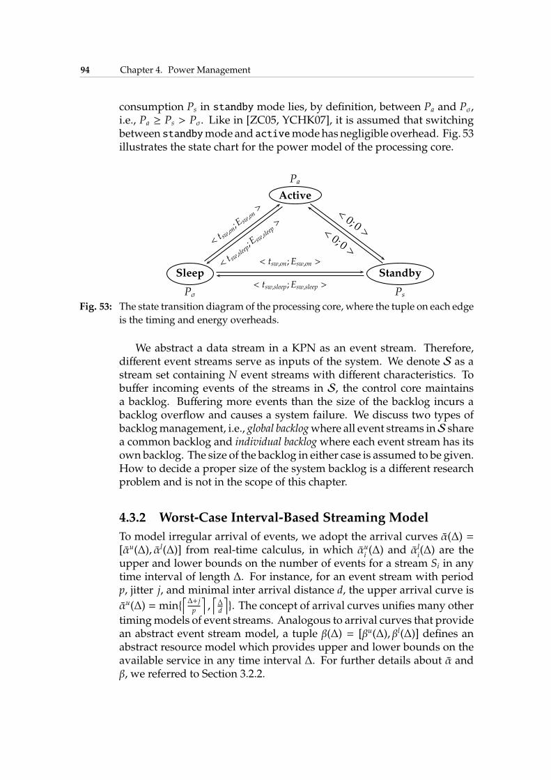
94 Chapter 4. Power Management
consumption Ps in standby mode lies, by definition, between Pa and Pσ,i.e., Pa ≥ Ps > Pσ. Like in [ZC05, YCHK07], it is assumed that switchingbetween standbymode and activemodehas negligible overhead. Fig. 53illustrates the state chart for the power model of the processing core.
Active
Pa
Standby
Ps
Sleep
Pσ
<0; 0 >
<0; 0 >
<t sw,sleep;E sw
,sleep>
< tsw,sleep;Esw,sleep >
<t sw,on;E sw
,on>
< tsw,on;Esw,on >
Fig. 53: The state transition diagram of the processing core, where the tuple on each edge
is the timing and energy overheads.
We abstract a data stream in a KPN as an event stream. Therefore,different event streams serve as inputs of the system. We denote S as astream set containing N event streams with different characteristics. Tobuffer incoming events of the streams in S, the control core maintainsa backlog. Buffering more events than the size of the backlog incurs abacklog overflow and causes a system failure. We discuss two types ofbacklogmanagement, i.e., global backlogwhere all event streams inS sharea common backlog and individual backlogwhere each event stream has itsown backlog. The size of the backlog in either case is assumed to be given.How to decide a proper size of the system backlog is a different researchproblem and is not in the scope of this chapter.
4.3.2 Worst-Case Interval-Based Streaming Model
To model irregular arrival of events, we adopt the arrival curves α(∆) =[αu(∆), αl(∆)] from real-time calculus, in which αu
i(∆) and αl
i(∆) are the
upper and lower bounds on the number of events for a stream Si in anytime interval of length ∆. For instance, for an event stream with periodp, jitter j, and minimal inter arrival distance d, the upper arrival curve is
αu(∆) = min{⌈∆+ j
p
⌉
,⌈∆d
⌉
}. The concept of arrival curves unifies many other
timingmodels of event streams. Analogous to arrival curves that providean abstract event stream model, a tuple β(∆) = [βu(∆), βl(∆)] defines anabstract resource model which provides upper and lower bounds on theavailable service in any time interval ∆. For further details about α andβ, we referred to Section 3.2.2.
4.3. System Model and Problem Definition 95
Note that an arrival curve αi(∆) specifies the number of events ofstream Si whereas a service curve β(∆) specifies the available amount ofservices in terms of time for an interval of length ∆. Therefore, αi(∆) hasto be transformed to αi(∆) to indicate the amount of computation timerequired for the arrived events in intervals. Suppose that the executiontime of any event in stream Si is wi. Then the transformation can be doneby αu
i= wi · αui , α
li= wi · αli and back by αu
i= ⌈αu/wi⌉, αli = ⌊α
l/wi⌋. Forvariable workloads in an event stream, our algorithms can be revisedslightly by adopting the variable workload model in Section 3.2.2.3.Moreover, the response time of an event in event stream Si must notexceed its specified relative deadline Di, where the response time of anevent is its finishing time minus the arrival time of the event. On thearrival of an event of stream Si at time t, the absolute deadline is t +Di.
4.3.3 Problem Definition
We explore how to effectively minimize the power consumption to servea stream set S by dynamic power management (DPM). Intuitively, staticpower can be reduced by a) turning the device to sleepmodewhen thereis no event to process, and b) staying at sleepmode as long as possible bypostponing the processing of arrived events. However, switching from/tosleepmode incurs both a timing and an energy overhead. Tomodel theseoverheads, we define a break-even time.
Def. 4: (Break Even Time) Suppose that a) switching the processing core to sleepmode takes tsw, sleep time and switching back to active/standby mode takestsw, on time, b) the corresponding energy consumption for the switching activitiesare Esw, sleep and Esw, on, and c) Ps and Pσ are the power consumption in thestandby and sleepmodes, respectively. The break-even time TBET is defined as:
TBETdef
= max{
tsw, on + tsw, sleep,Esw, on + Esw, sleep
Ps − Pσ
}
(4.1)
Consider the case that the processing core is switched to sleepmode.If the interval that the processing core can stay in sleep mode is shorterthan TBET, the mode-switch overhead is larger than the energy saving. Inthis case, amode switch does not pay off. On the other hand, retaining theprocessing core in sleepmode might incur backlog overflow or deadlinemisses for (burst) event arrivals in the near future. The question is whatis a proper moment to conduct a mode switch of the processing core.
We use the following notation: A schedule decides when to performa mode-switch of the processing core. A schedule is feasible if it is alwayspossible to meet the timing and backlog constraints of the system. Analgorithm is feasible if it always generates feasible scheduling decisions.
96 Chapter 4. Power Management
Therefore, the problem studied in this chapter is to determine a feasibleschedule a) when to turn the processing core to sleepmode to reduce the staticpower, and b) when to turn the processing core from sleep mode to activemode to serve events.
4.4 Real-Time Calculus Routines
To compute a feasible schedule for the processing core, real-timecalculus and real-time interface are applied. Within this context, theprocessing core is said to provide a guaranteed output service βG(∆).Correspondingly, a stream Si requests service demand βA(∆). To obtain afeasible schedule of theprocessing core that serves streamSi, the condition
βG(∆) ≥ βA(∆), ∀∆ ≥ 0 (4.2)
has to be fulfilled. In this section, we present how to construct properservice guarantees and demands such that (4.2) leads to a feasibleschedule.
4.4.1 Bounded Delay
Suppose that a service curve β(∆) can be constructed as a bounded delayfunction.
Def. 5: (Bounded Delay Service Curve) A bounded delay service curve is defined asfollows:
bdf (∆, τ)def= max
{
0, (∆ − τ)}
, ∀∆ ≥ 0, τ ≥ 0 (4.3)
where τ denote the sleep interval.
We say that a sleep interval is the accumulated time for which theprocessing core retains in sleep mode. In the case that the processingcore provides full service, i. e. , τ = 0, the processing core never switchesto sleepmode.
Def. 6: (Longest Feasible Sleep Interval) The longest feasible sleep interval τ∗ withrespect to a given service demand βA(∆) is thereby defined as:
τ∗ = max{
τ : bdf (∆, τ) ≥ βA(∆), ∀∆ ≥ 0}
(4.4)
Def. 7: (DeadlineServiceDemand)Suppose events in event streamSi are constrainedby a given relative deadline Di. To satisfy the required relative deadline Di, theminimal service demand β♭ of stream Si is
β♭(∆)def= αui (∆ −Di) (4.5)
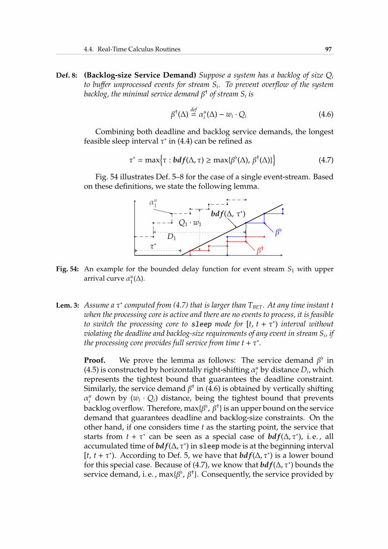
4.4. Real-Time Calculus Routines 97
Def. 8: (Backlog-size Service Demand) Suppose a system has a backlog of size Qi
to buffer unprocessed events for stream Si. To prevent overflow of the systembacklog, the minimal service demand β† of stream Si is
β†(∆)def= αui (∆) − wi ·Qi (4.6)
Combining both deadline and backlog service demands, the longestfeasible sleep interval τ∗ in (4.4) can be refined as
τ∗ = max{
τ : bdf (∆, τ) ≥ max{β♭(∆), β†(∆)}}
(4.7)
Fig. 54 illustrates Def. 5–8 for the case of a single event-stream. Basedon these definitions, we state the following lemma.
bdf (∆, τ∗)
τ∗D1
Q1 · w1
αu1
β♭
β†
b b
b b
b b
b b
b b
b b
b
b b
b b
b b
b
b
b b
b b
b b
b b
Fig. 54: An example for the bounded delay function for event stream S1 with upper
arrival curve αu1(∆).
Lem. 3: Assume a τ∗ computed from (4.7) that is larger than TBET. At any time instant twhen the processing core is active and there are no events to process, it is feasibleto switch the processing core to sleep mode for [t, t + τ∗) interval withoutviolating the deadline and backlog-size requirements of any event in stream Si, ifthe processing core provides full service from time t + τ∗.
Proof. We prove the lemma as follows: The service demand β♭ in(4.5) is constructed by horizontally right-shifting αu
iby distanceDi, which
represents the tightest bound that guarantees the deadline constraint.Similarly, the service demand β† in (4.6) is obtained by vertically shiftingαuidown by (wi · Qi) distance, being the tightest bound that prevents
backlog overflow. Therefore, max{β♭, β†} is an upper bound on the servicedemand that guarantees deadline and backlog-size constraints. On theother hand, if one considers time t as the starting point, the service thatstarts from t + τ∗ can be seen as a special case of bdf (∆, τ∗), i. e. , allaccumulated time of bdf (∆, τ∗) in sleepmode is at the beginning interval[t, t + τ∗). According to Def. 5, we have that bdf (∆, τ∗) is a lower boundfor this special case. Because of (4.7), we know that bdf (∆, τ∗) bounds theservice demand, i. e. , max{β♭, β†}. Consequently, the service provided by
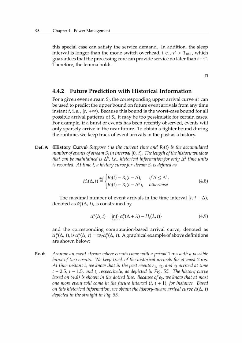
98 Chapter 4. Power Management
this special case can satisfy the service demand. In addition, the sleepinterval is longer than the mode-switch overhead, i. e. , τ∗ > TBET, whichguarantees that the processing core can provide service no later than t+τ∗.Therefore, the lemma holds.
�
4.4.2 Future Prediction with Historical Information
For a given event stream Si, the corresponding upper arrival curve αuican
be used to predict the upper bound on future event arrivals from any timeinstant t, i. e. , [t, +∞). Because this bound is the worst-case bound for allpossible arrival patterns of Si, it may be too pessimistic for certain cases.For example, if a burst of events has been recently observed, events willonly sparsely arrive in the near future. To obtain a tighter bound duringthe runtime, we keep track of event arrivals in the past as a history.
Def. 9: (History Curve) Suppose t is the current time and Ri(t) is the accumulatednumber of events of stream Si in interval [0, t). The length of the history windowthat can be maintained is ∆h, i.e., historical information for only ∆h time unitsis recorded. At time t, a history curve for stream Si is defined as
Hi(∆, t)def=
Ri(t) − Ri(t − ∆), if ∆ ≤ ∆h,
Ri(t) − Ri(t − ∆h), otherwise
(4.8)
The maximal number of event arrivals in the time interval [t, t + ∆),denoted as αu
i(∆, t), is constrained by
αui (∆, t) = infλ≥0
{
αui (∆ + λ) −Hi(λ, t)}
(4.9)
and the corresponding computation-based arrival curve, denoted asα u
i(∆, t), isαu
i(∆, t) = wi·αui (∆, t). Agraphical example of abovedefinitions
are shown below:
Ex. 6: Assume an event stream where events come with a period 1ms with a possibleburst of two events. We keep track of the historical arrivals for at most 2ms.At time instant t, we know that in the past events e1, e2, and e3 arrived at timet − 2.5, t − 1.5, and t, respectively, as depicted in Fig. 55. The history curvebased on (4.8) is shown in the dotted line. Because of e3, we know that at mostone more event will come in the future interval (t, t + 1), for instance. Basedon this historical information, we obtain the history-aware arrival curve α(∆, t)depicted in the straight in Fig. 55.
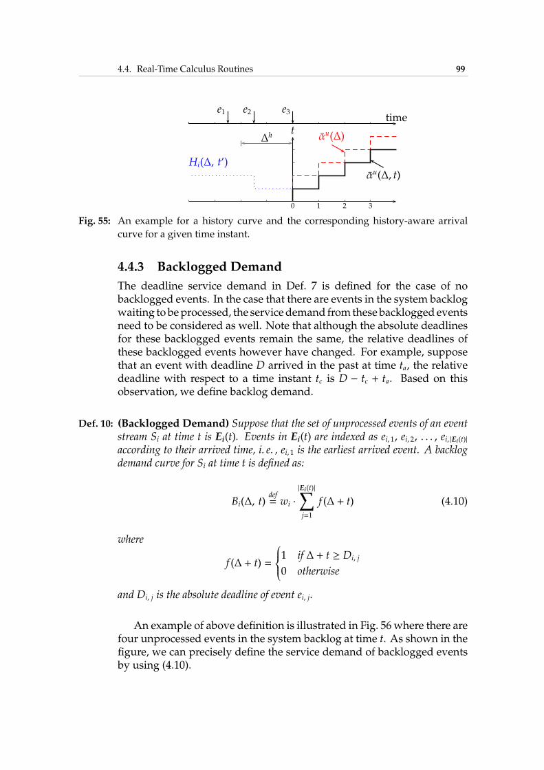
4.4. Real-Time Calculus Routines 99
ttime
e3e2e1
∆h
0 1 2 3
αu(∆)
αu(∆, t)Hi(∆, t′)
Fig. 55: An example for a history curve and the corresponding history-aware arrival
curve for a given time instant.
4.4.3 Backlogged Demand
The deadline service demand in Def. 7 is defined for the case of nobacklogged events. In the case that there are events in the system backlogwaiting to beprocessed, the servicedemand from these backlogged eventsneed to be considered as well. Note that although the absolute deadlinesfor these backlogged events remain the same, the relative deadlines ofthese backlogged events however have changed. For example, supposethat an event with deadline D arrived in the past at time ta, the relativedeadline with respect to a time instant tc is D − tc + ta. Based on thisobservation, we define backlog demand.
Def. 10: (Backlogged Demand) Suppose that the set of unprocessed events of an eventstream Si at time t is Ei(t). Events in Ei(t) are indexed as ei, 1, ei, 2, . . . , ei, |Ei(t)|
according to their arrived time, i. e. , ei, 1 is the earliest arrived event. A backlogdemand curve for Si at time t is defined as:
Bi(∆, t)def= wi ·
|Ei(t)|∑
j=1
f (∆ + t) (4.10)
where
f (∆ + t) =
1 if ∆ + t ≥ Di, j
0 otherwise
and Di, j is the absolute deadline of event ei, j.
An example of above definition is illustrated in Fig. 56 where there arefour unprocessed events in the system backlog at time t. As shown in thefigure, we can precisely define the service demand of backlogged eventsby using (4.10).
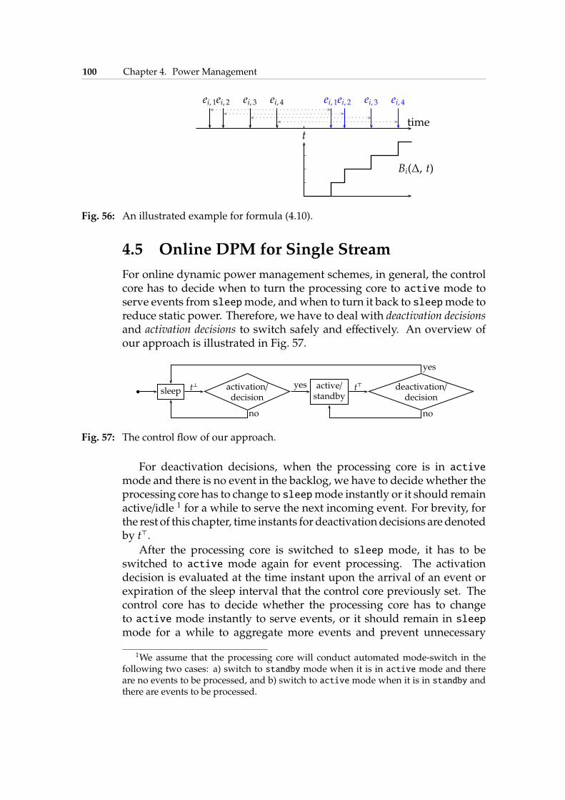
100 Chapter 4. Power Management
Bi(∆, t)
ttime
ei, 1 ei, 1ei, 2 ei, 2ei, 3 ei, 3ei, 4 ei, 4
Fig. 56: An illustrated example for formula (4.10).
4.5 Online DPM for Single Stream
For online dynamic power management schemes, in general, the controlcore has to decide when to turn the processing core to active mode toserve events from sleepmode, andwhen to turn it back to sleepmode toreduce static power. Therefore, we have to deal with deactivation decisionsand activation decisions to switch safely and effectively. An overview ofour approach is illustrated in Fig. 57.
. sleep activation/decision
active/standby
deactivation/decision
t⊥ yes t⊤
yes
nono
Fig. 57: The control flow of our approach.
For deactivation decisions, when the processing core is in activemode and there is no event in the backlog, we have to decide whether theprocessing core has to change to sleepmode instantly or it should remainactive/idle 1 for a while to serve the next incoming event. For brevity, forthe rest of this chapter, time instants for deactivationdecisions aredenotedby t⊤.
After the processing core is switched to sleep mode, it has to beswitched to active mode again for event processing. The activationdecision is evaluated at the time instant upon the arrival of an event orexpiration of the sleep interval that the control core previously set. Thecontrol core has to decide whether the processing core has to changeto active mode instantly to serve events, or it should remain in sleepmode for a while to aggregate more events and prevent unnecessary
1We assume that the processing core will conduct automated mode-switch in thefollowing two cases: a) switch to standby mode when it is in active mode and thereare no events to be processed, and b) switch to activemode when it is in standby andthere are events to be processed.
4.5. Online DPM for Single Stream 101
mode switches. For brevity, for the rest of this chapter, time instants foractivation decisions are denoted by t⊥.
In this section, we present our online algorithms that are applied to thecontrol core and minimize static power consumption of the processingcore. The assumption of our approach is that the timing and backlogconstraints of system can always be guaranteed if the processing coreprovides full service all the time, i.e., the processing core never turns tosleep mode. For simplicity, we first consider only the case of a singleevent stream S1. We present how to deal with the deactivation decisionand then propose two methods for activation decision. The solutions formultiple event streams are presented in the subsequent two sections.
4.5.1 Deactivation Algorithm
The History-Aware Deactivation (HAD) algorithm analyzes whether theprocessing core should be turned to sleep mode from active mode.The principle is to switch the processing core only when energy savingsare possible. One obvious fact is that as long as there are events in thesystem backlog, the processing core can be kept busy in active modeuntil all backlogged events are processed. In this case, no static poweris wasted and any mode-switch will introduce an additional time andenergy overhead. In order to reduce the mode-switch overhead, thedeactivation decision therebymakes sense only when the processing coreis in active or standby mode while there is no new arrival of events aswell as no event in system backlog. Suppose that t⊤ is such a time instant.
Turning the processing core instantly at time t⊤ to sleep mode,however, does still not always help. The reason is that we pay a time andenergy overhead for each mode switch. In the case that there are eventsarriving in the very near future, the processing core has to be switched toactivemode again to process these events. If the energy savings obtainedfrom a short sleep interval cannot outweigh the switching overhead, thismode switch only introduces additional energy consumption. Therefore,the idea is firstly to compute the maximal possible sleep interval τ∗
and check whether this τ∗ is sufficient to cover the break-even time.Specifically, we calculate the arrival curve αu
1(∆, t⊤) at time t⊤ by (4.9)
and refine the service demands in (4.5) and (4.6) as
β♭(∆) = αu1(∆ −D1, t⊤) (4.11)
β†(∆) = αu1(∆, t⊤) −Q1 · w1 (4.12)
By applying (4.11) and (4.12) to (4.7), the maximal sleep interval τ∗ iscomputed. If τ∗ is larger than TBET, the processing core is switched tosleep mode at time t⊤. Otherwise, the processing core is retained in
102 Chapter 4. Power Management
active/standby mode. The pseudo code of the algorithm is shown inAlgorithm 3.
Algorithm 3 HAD deactivation
procedure at time instant t⊤:1: compute τ∗ of (4.7) by β♭ and β† in (4.11) and (4.12);2: if τ∗ > TBET then3: deactivate the processing core;4: end if
The algorithm leads to the following theorem:
Thm. 3: Algorithm HAD guarantees a feasible scheduling upon a deactivation decisionat any time t⊤ for a single event-stream system if the processing core providesfull service starting from time t⊤ + τ∗, where τ∗ is computed from line 1 of thealgorithm.
Proof. We prove this theorem by contradiction. At any time instant t⊤
at which Algorithm HAD decides to deactivate the processing core, thelatest activation time to prevent constraint violations is t⊤ + τ∗. Supposeat a later time instant t⊤ +λ, the deadline of an event which comes withinthe interval [t⊤, t⊤+λ) is missed. We denote the number of events arrivedwithin this interval as u. Because of the deadline missing, the servicedemand u ·w1 in this interval is larger than our constructed service supplybdf (λ, τ∗) which actually bounds the service demand of the maximumnumber of events that can arrive, i.e., w1 · αu1(λ, t
⊤). The inequalityu > αu
1(λ, t⊤) contradicts the definition in (4.9), however. Therefore, the
theorem holds.
�
4.5.2 Activation Algorithms
Once the processing core is in sleep mode, the control core needs toswitch it back to active mode at a later moment for event processing.How to decide the actual switch moment needs more consideration. Onthe one hand, it is preferable to aggregate as many events as possiblefor each switch operation to not only reduce the standby period but alsominimize the number of switch operations. On the other hand, the real-time constraints of the aggregated and future events need to be respected.In addition, a polling mechanism is not desirable which will overload thecontrol core. In this section, we present two algorithms, namely worst-case-greedy (WCG) algorithmand event-driven-greedy (EDG) algorithm,for activation scheduling decisions. The differences between these twoalgorithms are:
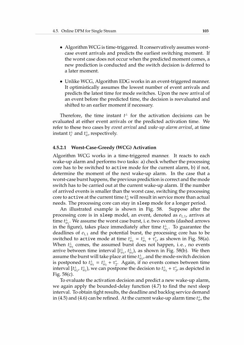
4.5. Online DPM for Single Stream 103
• AlgorithmWCG is time-triggered. It conservatively assumesworst-case event arrivals and predicts the earliest switching moment. Ifthe worst case does not occur when the predicted moment comes, anew prediction is conducted and the switch decision is deferred toa later moment.
• Unlike WCG, Algorithm EDG works in an event-triggered manner.It optimistically assumes the lowest number of event arrivals andpredicts the latest time for mode switches. Upon the new arrival ofan event before the predicted time, the decision is reevaluated andshifted to an earlier moment if necessary.
Therefore, the time instant t⊥ for the activation decisions can beevaluated at either event arrivals or the predicted activation time. Werefer to these two cases by event arrival and wake-up alarm arrival, at timeinstant t⊥e and t⊥w, respectively.
4.5.2.1 Worst-Case-Greedy (WCG) Activation
Algorithm WCG works in a time-triggered manner. It reacts to eachwake-up alarm and performs two tasks: a) check whether the processingcore has to be switched to active mode for the current alarm, b) if not,determine the moment of the next wake-up alarm. In the case that aworst-case burst happens, the previous prediction is correct and themodeswitch has to be carried out at the current wake-up alarm. If the numberof arrived events is smaller than the worst case, switching the processingcore to active at the current time t⊥w will result in servicemore than actualneeds. The processing core can stay in sleepmode for a longer period.
An illustrated example is shown in Fig. 58. Suppose after theprocessing core is in sleep model, an event, denoted as e1, 1, arrives attime t⊥w1
. We assume the worst case burst, i. e. two events (dashed arrowsin the figure), takes place immediately after time t⊥w1
. To guarantee thedeadlines of e1, 1 and the potential burst, the processing core has to beswitched to active mode at time t⊥w2
= t⊥w1+ τ∗
1, as shown in Fig. 58(a).
When t⊥w2comes, the assumed burst does not happen, i. e. , no events
arrive between time interval [t⊥w1, t⊥w2
), as shown in Fig. 58(b). We thenassume the burst will take place at time t⊥w2
, and themode-switch decisionis postponed to t⊥w3
= t⊥w2+ τ∗2. Again, if no events comes between time
interval [t⊥w2, t⊥w3
), we can postpone the decision to t⊥w3+ τ∗3, as depicted in
Fig. 58(c).To evaluate the activation decision and predict a new wake-up alarm,
we again apply the bounded-delay function (4.7) to find the next sleepinterval. To obtain tight results, the deadline and backlog service demandin (4.5) and (4.6) can be refined. At the current wake-up alarm time t⊥w, the
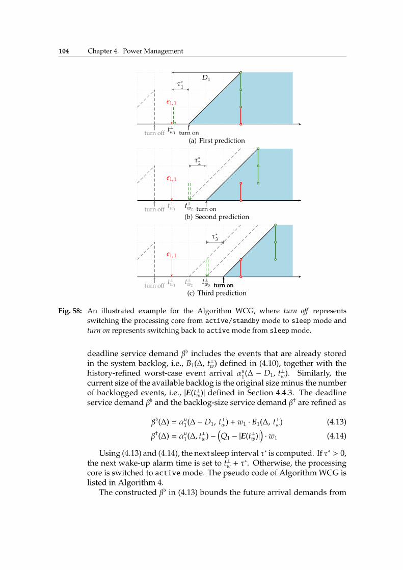
104 Chapter 4. Power Management
turn off
D1
e1, 1
t⊥w1 turn on
τ∗1
(a) First prediction
turn off
e1, 1
t⊥w2t⊥w1 turn on
τ∗2
(b) Second prediction
turn off
e1, 1
t⊥w3t⊥w1
t⊥w2
τ∗3
turn onturn on
(c) Third prediction
Fig. 58: An illustrated example for the Algorithm WCG, where turn off represents
switching the processing core from active/standby mode to sleep mode and
turn on represents switching back to activemode from sleepmode.
deadline service demand β♭ includes the events that are already storedin the system backlog, i.e., B1(∆, t⊥w) defined in (4.10), together with thehistory-refined worst-case event arrival αu
1(∆ − D1, t⊥w). Similarly, the
current size of the available backlog is the original size minus the numberof backlogged events, i.e., |E(t⊥w)| defined in Section 4.4.3. The deadlineservice demand β♭ and the backlog-size service demand β† are refined as
β♭(∆) = αu1(∆ −D1, t⊥w) + w1 · B1(∆, t
⊥w) (4.13)
β†(∆) = αu1(∆, t⊥w) −(
Q1 − |E(t⊥w)|)
· w1 (4.14)
Using (4.13) and (4.14), the next sleep interval τ∗ is computed. If τ∗ > 0,the next wake-up alarm time is set to t⊥w + τ
∗. Otherwise, the processingcore is switched to activemode. The pseudo code of AlgorithmWCG islisted in Algorithm 4.
The constructed β♭ in (4.13) bounds the future arrival demands from
4.5. Online DPM for Single Stream 105
Algorithm 4WCG activation
procedure event arrival at time t⊥e :1: do nothing;
procedure wake-up alarm arrival at time t⊥w:1: compute τ∗ of (4.7) with β♭ and β† by (4.13) and (4.14);2: if τ∗ > 0 then3: new wake-up alarm at time t⊥w ← t⊥w + τ
∗;4: else5: switch processing core to activemode;6: end if
t⊥w on and β† in (4.14) guarantees the system backlog from overflowing,leading to following theorem:
Thm. 4: AlgorithmWCG guarantees a feasible scheduling upon an activation decision atany wake-up alarm time t⊥w for single event-stream system, if the processing coreprovides full service from time t⊥w on.
We omit the proof due to the similarity to Theorem 1. AlgorithmWCG is effective in the sense that it greedily extends the sleep period aslong as a scheduling decision is feasible. It is also efficient when actualevent arrivals are close to the worst case, where the reevaluation of thewake-up alarm time does not take place often. Furthermore, the numberof reevaluation is bounded by αu
1(D1 − w1).
The last question is when to set the first wake-up alarm. There are twopossibilities: a) at the time of the first arrived event after the processingcore is deactivated, and b) at the deactivation time instant t⊤ + τ∗ (τ∗
is computed by (4.11), (4.12), and (4.7) in the HAD algorithm). Bothapproaches will result in feasible schedule. For consistency, we adopt thesecond approach and thus AlgorithmWCG is purely time-driven.
4.5.2.2 Event-Driven-Greedy (EDG) Activation
In contrast to Algorithm WCG that predicts the earliest wake-up alarmtime t⊥w, Algorithm EDG predicts the latest one. It computes the latestmoment by assuming the lowest number of event arrivals in the nearfuture. Unlike Algorithm WCG where the evaluation of the activationdecisions takes place upon each wake-up alarm arrives, the decision hereis refined upon event arrivals.
At time t⊥e1, i at which an event e1, i arrives, it is not obvious when thecorresponding latest wake-up alarm t⊥w will be. One intuitive guess ist⊥e1, i +D1 − w1. This time instant is however too optimistic except for thefirst event e1, 1 after the processing core has been deactivated. Our EDG
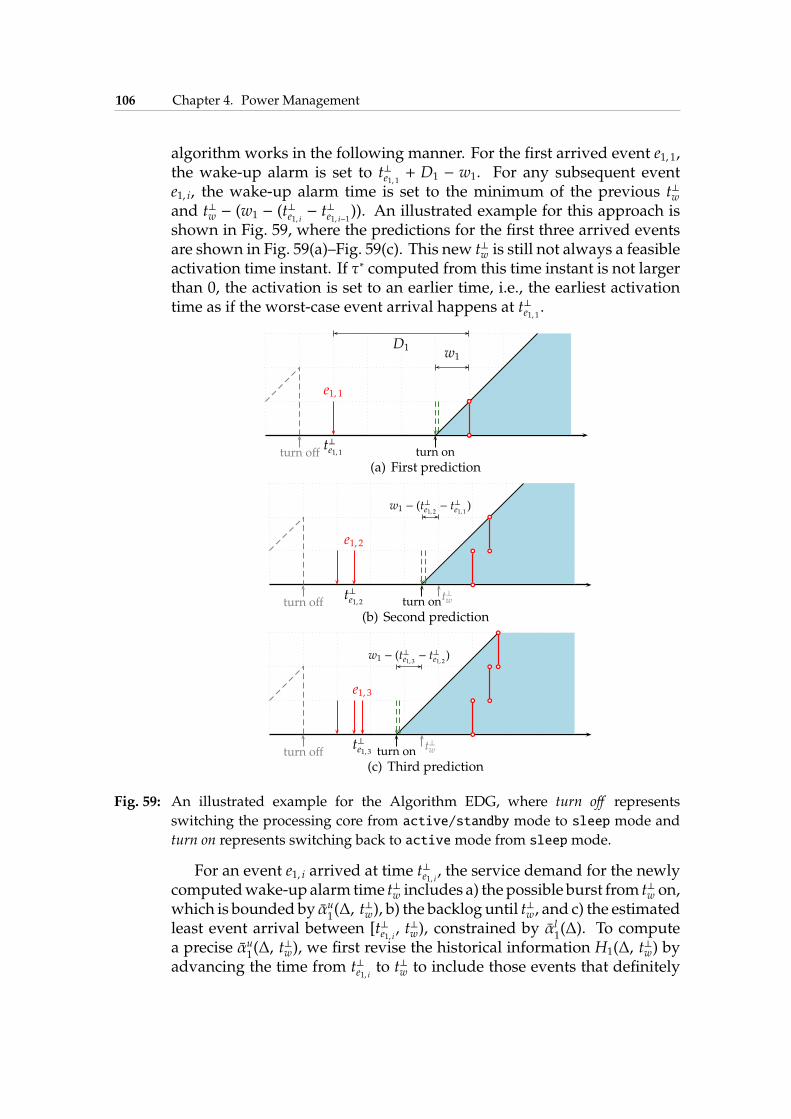
106 Chapter 4. Power Management
algorithm works in the following manner. For the first arrived event e1, 1,the wake-up alarm is set to t⊥e1, 1 + D1 − w1. For any subsequent evente1, i, the wake-up alarm time is set to the minimum of the previous t⊥wand t⊥w − (w1 − (t⊥e1, i − t⊥e1, i−1)). An illustrated example for this approach isshown in Fig. 59, where the predictions for the first three arrived eventsare shown in Fig. 59(a)–Fig. 59(c). This new t⊥w is still not always a feasibleactivation time instant. If τ∗ computed from this time instant is not largerthan 0, the activation is set to an earlier time, i.e., the earliest activationtime as if the worst-case event arrival happens at t⊥e1, 1 .
turn off
e1, 1
t⊥e1, 1 turn on
D1 w1
(a) First prediction
turn off
e1, 2
t⊥e1, 2 turn ont⊥w
w1 − (t⊥e1, 2 − t⊥e1, 1 )
(b) Second prediction
turn off
e1, 3
t⊥e1, 3 t⊥wturn on
w1 − (t⊥e1, 3 − t⊥e1, 2 )
(c) Third prediction
Fig. 59: An illustrated example for the Algorithm EDG, where turn off represents
switching the processing core from active/standby mode to sleep mode and
turn on represents switching back to activemode from sleepmode.
For an event e1, i arrived at time t⊥e1, i , the service demand for the newlycomputedwake-up alarm time t⊥w includes a) thepossible burst from t⊥w on,which is bounded by αu
1(∆, t⊥w), b) the backlog until t
⊥w, and c) the estimated
least event arrival between [t⊥e1, i , t⊥w), constrained by αl
1(∆). To compute
a precise αu1(∆, t⊥w), we first revise the historical information H1(∆, t⊥w) by
advancing the time from t⊥e1, i to t⊥w to include those events that definitely
4.5. Online DPM for Single Stream 107
have to come between [t⊥e1,i , t⊥w). We denote such a trace as H′(∆, t⊥w):
H′1(∆, t⊥w) =
αl1(ǫ) − αl
1(ǫ − ∆), if∆ < ǫ,
H1(∆, t⊥e1,i) + αl1(ǫ), if ǫ < ∆ < ∆h − ǫ,
H1(∆h − ǫ, t⊥e1,i) + α
l1(ǫ), otherwise,
(4.15)
where ǫ = t⊥w − t⊥e1, i for brevity and ∆h is length of the history window.The curve H′
1can be considered as the concatenation of the historical
information H1 until t⊥e1, i and the time inversion of αl1in the interval
[0, ǫ). The worst-case arrival curve after time t⊥w with the new historicalinformation H′
1is
αu1(∆, t⊥w) = inf
λ≥0
{
αu1(∆ + λ) −H′1(λ, t⊥w)}
(4.16)
and αu1(∆, t⊥w) = w1 · αu1(∆, t
⊥w).
The corresponding backlog demand curve that expresses the esti-mated lowest number of arrival events within the interval [t⊥e1,i , t
⊥w) is
B′1(∆, t⊥w)
def= w1 ·
|E1(t)|+αl1(ǫ)∑
j=1
f (∆ + t⊥w) (4.17)
where
f (∆ + t⊥w) =
1 if ∆ + t⊥w ≥ D1, j
0 otherwise
and D1, j is the absolute deadline of event e1, j and ǫ = t⊥w − t⊥e1, i .
With the refined historical information and backlog demand, the twoservice demands β♭ and β† are refined as:
β♭(∆) = αu1(∆ −D1, t⊥w) + w1 · B
′1(∆, t
⊥w) (4.18)
β†(∆) = αu1(∆, t⊥w) −(
Q − |E(t⊥)| − αl1(ǫ))
· w1 (4.19)
By applying (4.18) and (4.19), the sleep interval τ∗ in (4.7) is computedfor event e1, i. If τ∗ > 0, the wake-up alarm is valid. Otherwise, thenew wake-up alarm is set to an earlier moment. The pseudo code of thealgorithm is depicted in Algorithm 5.
Thm. 5: Algorithm EDG guarantees a feasible scheduling upon an activation decision atany wake-up alarm time t⊥w for single event-stream system, if the processing coreprovides full service starting from time t⊥w.
108 Chapter 4. Power Management
Algorithm 5 EDG activation
procedure event arrival at time t⊥e1, i :1: if t⊥e1, i − t⊥e1, i−1 < w1 then2: t⊥w ← t⊥w − (w1 − (t⊥e1, i − t⊥e1, i−1))3: end if4: calculate τ∗ at time t⊥w by (4.15–4.19);5: if τ∗ ≤ 0 then6: t⊥w ← t⊥e1, 1 + τ
⊥, where τ⊥ computed from (4.5) – (4.7)7: end if
procedure wake-up alarm arrival at time t⊥w:1: activate the processing core;
Proof. We differentiate between two mode switch decisions: when thecondition in line 5 is fulfilled and when this is not the case. When thecondition is not fulfilled, the feasibility of the decision is guaranteed by(4.15)–(4.19) where the actually arrived events before time instant t⊥w andthe potential burst afterwards are both considered in each evaluation. Inthe case that the condition in line 5 is fulfilled, we need to prove thatthe arrival time t⊥e1, i of event e1, i is always earlier than t⊥e1, 1 + τ
⊥. For timeinstant t⊥e1, 1 at which e1, 1 arrives, the maximum number of events thatcan be stored in the system backlog is min{Q1, αu1(τ
⊥) − 1}, denoted as u.Based on the construction in line 1, τ∗ ≤ 0 is only fulfilled if the numberof arrived events reaches this maximum. According to the subadditivityof an upper arrival curve and the linearity of the bounded delay servicecurve, the time interval to generate u events is bounded by τ⊥, i.e., theinequality (αu)−1(τ⊥) > u always holds2. Therefore, t⊥e1, 1+τ
⊥ > t⊥e1, i . Becauset⊥e1, 1 + τ
⊥ assumes that the worst-case event arrivals happen at the timeinstant of the arrival of the first event after the processing core is switchedto sleep mode, switching the processing core to active mode at thistime always results in a feasible scheduling decision. As the schedulingdecisions are feasible for both cases, the theorem holds.
�
According to Thm. 5, Algorithm EDG results in a feasible schedule.The algorithm is efficient as well. It is designed for scenarios whereevents come sparsely and the worst case seldom occurs. In suchscenarios, the pessimistic decision, i.e., the condition in line 5 is fulfilled,takes place seldom. In addition, the theoretical upper bound of thenumber on reevaluations is min{Q1, αu1(τ
⊥)}. In practice, the number ofreevaluations is approximately equal to the number of actually arrived
2Symbol (αu)−1 represents the inverse function of αu.
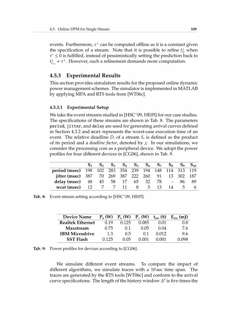
4.5. Online DPM for Single Stream 109
events. Furthermore, τ⊥ can be computed offline as it is a constant giventhe specification of a stream. Note that it is possible to refine t⊥w whenτ∗ ≤ 0 is fulfilled, instead of pessimistically setting the prediction back tot⊥e1,1 + τ
⊥. However, such a refinement demands more computation.
4.5.3 Experimental Results
This section provides simulation results for the proposed online dynamicpowermanagement schemes. The simulator is implemented inMATLABby applying MPA and RTS tools from [WT06c].
4.5.3.1 Experimental Setup
We take the event streams studied in [HSC+09, HE05] for our case studies.The specifications of these streams are shown in Tab. 8. The parametersperiod, jitter, and delay are used for generating arrival curves definedin Section 4.3.2 and wcet represents the worst-case execution time of anevent. The relative deadline Di of a stream Si is defined as the productof its period and a deadline factor, denoted by χ. In our simulations, weconsider the processing core as a peripheral device. We adopt the powerprofiles for four different devices in [CG06], shown in Tab. 9.
S1 S2 S3 S4 S5 S6 S7 S8 S9 S10
period (msec) 198 102 283 354 239 194 148 114 313 119jitter (msec) 387 70 269 387 222 260 91 13 302 187delay (msec) 48 45 58 17 65 32 78 - 86 89wcet (msec) 12 7 7 11 8 5 13 14 5 6
Tab. 8: Event stream setting according to [HSC+09, HE05].
Device Name Pa (W) Ps (W) Pσ (W) tsw (S) Esw (mJ)
Realtek Ethernet 0.19 0.125 0.085 0.01 0.8Maxstream 0.75 0.1 0.05 0.04 7.6
IBM Microdrive 1.3 0.5 0.1 0.012 9.6SST Flash 0.125 0.05 0.001 0.001 0.098
Tab. 9: Power profiles for devices according to [CG06].
We simulate different event streams. To compare the impact ofdifferent algorithms, we simulate traces with a 10 sec time span. Thetraces are generated by the RTS tools [WT06c] and conform to the arrivalcurve specifications. The length of the history window∆h is five times the
110 Chapter 4. Power Management
period of an event stream. We evaluate two DPM schemes, i.e., switchingto sleep with the HAD algorithm and switching back with the WCG orEDG algorithm, denoted as WCG-HAD and EDG-HAD. To show theeffects of our schemes, we report the average idle power that is computedas the total idle energy consumption divided by the time span of thesimulation. The average idle power is formally defined as follows:
Def. 11: (Average Idle Power Consumption) Suppose that: Esw, on and Esw, slepp arethe energy overheads for the switches to active and sleep modes, respectively;Con and Csleep are the total numbers of switches to active and sleep modes,respectively; Ton, sum the sum of all the time intervals in which the device stays inactive/standby modes; and Pσ is the power consumption in standby mode.The average idle power consumption is defined as:
Esw, on · Con + Esw, sleep · Csleep + Ton, sum · Pσ
total_time_span(4.20)
For comparison, two other power management schemes describedin 4.7 are measured as well, i.e., a periodic scheme (OPT) and anaive event-driven scheme (ED). The OPT scheme is a periodic powermanagement (PPM) scheme which controls the processing core with afixed on-off period. The lengths of the on and off periods are optimallycomputed with respect to the average idle power by an offline algorithmpresented in the upcoming Section 4.7. The ED scheme turns on theprocessing core whenever an event arrives and turns off when theprocessing core becomes idle. Note that OPT does not consider the sizeof the system backlog. For a fair comparison, we smooth out the effectof a small backlog-size by setting the backlog size to a relatively largenumber, i.e., 60 events for this experiment.
4.5.3.2 Results
First, we show the effectiveness of the proposed WCG-HAD and EDG-HAD schemes comparing to the OPT and ED schemes. Fig. 60 showsthe normalized values of average idle power with respect to OPT for thestreams in Tab. 8 individually processed on the four devices in Tab. 9. Asdepicted in the figure, both schemes proposed in this section outperformthe pure event-driven scheme as well as the OPT periodic scheme for allcases. On average, 25% of the average idle power with respect to OPT issaved for the deadline factor χ = 1.6.
In general, a small wcet/period ratio results in higher idle powersavings, as the cases for event streams S3, S4, S5, and S9. Counter-examples are event streams S2, S7, and S8. Event stream S8 has thelargest wcet/period ratio, conducting the worst idle power savings for
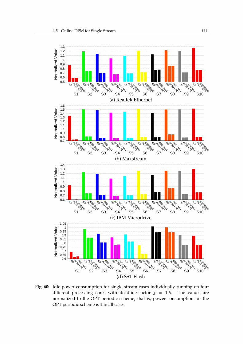
4.5. Online DPM for Single Stream 111
0.5 0.6 0.7 0.8 0.9
1 1.1 1.2 1.3
ED WCG-HAD
EDG-HAD
ED WCG-HAD
EDG-HAD
ED WCG-HAD
EDG-HAD
ED WCG-HAD
EDG-HAD
ED WCG-HAD
EDG-HAD
ED WCG-HAD
EDG-HAD
ED WCG-HAD
EDG-HAD
ED WCG-HAD
EDG-HAD
ED WCG-HAD
EDG-HAD
ED WCG-HAD
EDG-HAD
Nor
mal
ized
Val
ue
S10S9S8S7S6S5S4S3S2S1
(a) Realtek Ethernet
0.7 0.8 0.9
1 1.1 1.2 1.3 1.4 1.5 1.6
ED WCG-HAD
EDG-HAD
ED WCG-HAD
EDG-HAD
ED WCG-HAD
EDG-HAD
ED WCG-HAD
EDG-HAD
ED WCG-HAD
EDG-HAD
ED WCG-HAD
EDG-HAD
ED WCG-HAD
EDG-HAD
ED WCG-HAD
EDG-HAD
ED WCG-HAD
EDG-HAD
ED WCG-HAD
EDG-HAD
Nor
mal
ized
Val
ue
S10S9S8S7S6S5S4S3S2S1
(b) Maxstream
0.6 0.7 0.8 0.9
1 1.1 1.2 1.3 1.4
ED WCG-HAD
EDG-HAD
ED WCG-HAD
EDG-HAD
ED WCG-HAD
EDG-HAD
ED WCG-HAD
EDG-HAD
ED WCG-HAD
EDG-HAD
ED WCG-HAD
EDG-HAD
ED WCG-HAD
EDG-HAD
ED WCG-HAD
EDG-HAD
ED WCG-HAD
EDG-HAD
ED WCG-HAD
EDG-HAD
Nor
mal
ized
Val
ue
S10S9S8S7S6S5S4S3S2S1
(c) IBM Microdrive
0.6 0.65 0.7
0.75 0.8
0.85 0.9
0.95 1
1.05
ED WCG-HAD
EDG-HAD
ED WCG-HAD
EDG-HAD
ED WCG-HAD
EDG-HAD
ED WCG-HAD
EDG-HAD
ED WCG-HAD
EDG-HAD
ED WCG-HAD
EDG-HAD
ED WCG-HAD
EDG-HAD
ED WCG-HAD
EDG-HAD
ED WCG-HAD
EDG-HAD
ED WCG-HAD
EDG-HAD
Nor
mal
ized
Val
ue
S10S9S8S7S6S5S4S3S2S1
(d) SST Flash
Fig. 60: Idle power consumption for single stream cases individually running on four
different processing cores with deadline factor χ = 1.6. The values are
normalized to the OPT periodic scheme, that is, power consumption for the
OPT periodic scheme is 1 in all cases.
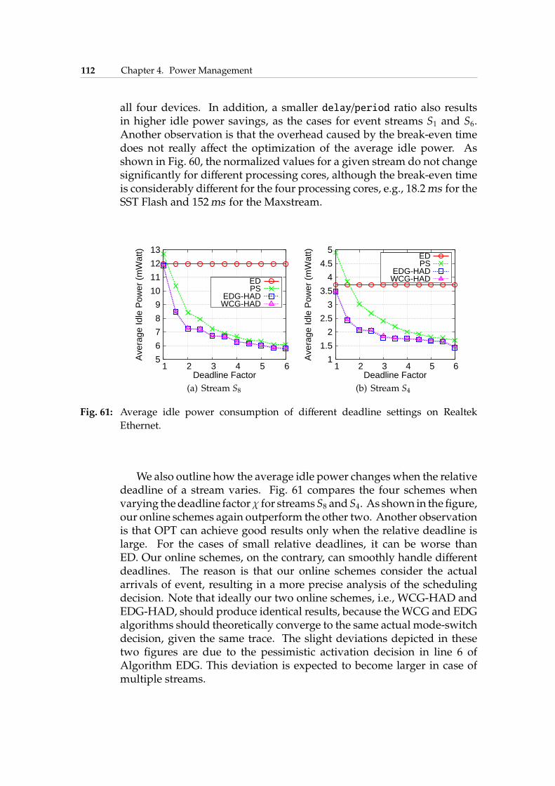
112 Chapter 4. Power Management
all four devices. In addition, a smaller delay/period ratio also resultsin higher idle power savings, as the cases for event streams S1 and S6.Another observation is that the overhead caused by the break-even timedoes not really affect the optimization of the average idle power. Asshown in Fig. 60, the normalized values for a given stream do not changesignificantly for different processing cores, although the break-even timeis considerably different for the four processing cores, e.g., 18.2ms for theSST Flash and 152ms for the Maxstream.
5
6
7
8
9
10
11
12
13
1 2 3 4 5 6
Ave
rage
Idle
Pow
er (
mW
att)
Deadline Factor
EDPS
EDG-HADWCG-HAD
(a) Stream S8
1
1.5
2
2.5
3
3.5
4
4.5
5
1 2 3 4 5 6
Ave
rage
Idle
Pow
er (
mW
att)
Deadline Factor
EDPS
EDG-HADWCG-HAD
(b) Stream S4
Fig. 61: Average idle power consumption of different deadline settings on Realtek
Ethernet.
We also outline how the average idle power changes when the relativedeadline of a stream varies. Fig. 61 compares the four schemes whenvarying thedeadline factorχ for streamsS8 andS4. As shown in thefigure,our online schemes again outperform the other two. Another observationis that OPT can achieve good results only when the relative deadline islarge. For the cases of small relative deadlines, it can be worse thanED. Our online schemes, on the contrary, can smoothly handle differentdeadlines. The reason is that our online schemes consider the actualarrivals of event, resulting in a more precise analysis of the schedulingdecision. Note that ideally our two online schemes, i.e., WCG-HAD andEDG-HAD, should produce identical results, because theWCG and EDGalgorithms should theoretically converge to the same actual mode-switchdecision, given the same trace. The slight deviations depicted in thesetwo figures are due to the pessimistic activation decision in line 6 ofAlgorithm EDG. This deviation is expected to become larger in case ofmultiple streams.
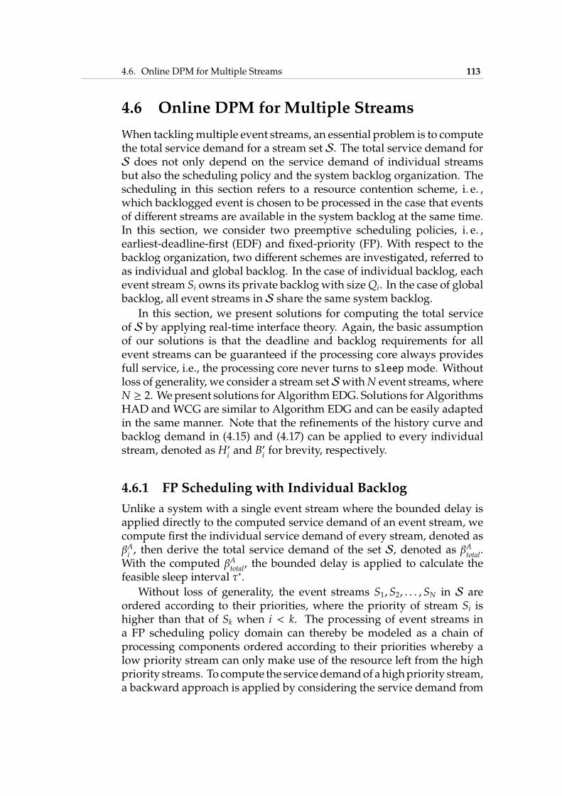
4.6. Online DPM for Multiple Streams 113
4.6 Online DPM for Multiple Streams
When tacklingmultiple event streams, an essential problem is to computethe total service demand for a stream set S. The total service demand forS does not only depend on the service demand of individual streamsbut also the scheduling policy and the system backlog organization. Thescheduling in this section refers to a resource contention scheme, i. e. ,which backlogged event is chosen to be processed in the case that eventsof different streams are available in the system backlog at the same time.In this section, we consider two preemptive scheduling policies, i. e. ,earliest-deadline-first (EDF) and fixed-priority (FP). With respect to thebacklog organization, two different schemes are investigated, referred toas individual and global backlog. In the case of individual backlog, eachevent stream Si owns its private backlog with sizeQi. In the case of globalbacklog, all event streams in S share the same system backlog.
In this section, we present solutions for computing the total serviceof S by applying real-time interface theory. Again, the basic assumptionof our solutions is that the deadline and backlog requirements for allevent streams can be guaranteed if the processing core always providesfull service, i.e., the processing core never turns to sleepmode. Withoutloss of generality, we consider a stream setSwithN event streams, whereN ≥ 2. Wepresent solutions forAlgorithmEDG. Solutions forAlgorithmsHAD and WCG are similar to Algorithm EDG and can be easily adaptedin the same manner. Note that the refinements of the history curve andbacklog demand in (4.15) and (4.17) can be applied to every individualstream, denoted as H′
iand B′
ifor brevity, respectively.
4.6.1 FP Scheduling with Individual Backlog
Unlike a system with a single event stream where the bounded delay isapplied directly to the computed service demand of an event stream, wecompute first the individual service demand of every stream, denoted asβAi, then derive the total service demand of the set S, denoted as βA
total.
With the computed βAtotal
, the bounded delay is applied to calculate thefeasible sleep interval τ∗.
Without loss of generality, the event streams S1,S2, . . . ,SN in S areordered according to their priorities, where the priority of stream Si ishigher than that of Sk when i < k. The processing of event streams ina FP scheduling policy domain can thereby be modeled as a chain ofprocessing components ordered according to their priorities whereby alow priority stream can only make use of the resource left from the highpriority streams. To compute the servicedemandof ahighpriority stream,a backward approach is applied by considering the service demand from
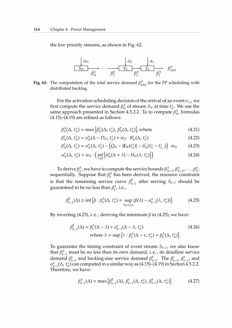
114 Chapter 4. Power Management
the low priority streams, as shown in Fig. 62.
SN. . . S2 S1 βA
total
αN α2 α1
βAN βA3 βA2 βA1
Fig. 62: The computation of the total service demand βAtotal
for the FP scheduling with
distributed backlog.
For the activation scheduling decision of the arrival of an event e1, i, wefirst compute the service demand βAN of stream SN at time t⊥w. We use thesame approach presented in Section 4.5.2.2. To to compute βAN, formulas(4.15)–(4.19) are refined as follows:
βAN(∆, t⊥w) = max
{
β♭N(∆, t⊥w), β
†N(∆, t
⊥w)}
,where (4.21)
β♭N(∆, t⊥w) = α
uN(∆ −DN, t
⊥w) + wN · B
′N(∆, t
⊥w) (4.22)
β†N(∆, t⊥w) = α
uN(∆, t
⊥w) −(
QN − |EN(t⊥w)| − α
lN(t⊥w − t⊥e1, i)
)
· wN (4.23)
αuN(∆, t⊥w) = wN ·
(
infλ≥0
{
αuN(∆ + λ) −HN(λ, t⊥w)})
(4.24)
To derive βA1, we have to compute the service bounds βA
N−1, βAN−2, . . . , β
A2 ,
sequentially. Suppose that βAkhas been derived, the resource constraint
is that the remaining service curve β♯k−1
after serving Sk−1 should be
guaranteed to be no less than βAk, i.e.,
β♯k−1
(∆) ≥ inf{
β : βAk (∆, t⊥w) = sup
0≤λ≤∆
{β(λ) − αuk−1(λ, t⊥w)}}
(4.25)
By inverting (4.25), i. e. , deriving the minimum β in (4.25), we have:
β♯k−1
(∆) = βAk (∆ − λ) + αuk−1(∆ − λ, t
⊥w) (4.26)
where λ = sup{
τ : βAk (∆ − τ, t⊥w) = β
Ak (∆, t
⊥w)}
To guarantee the timing constraint of event stream Sk−1, we also knowthat βA
k−1must be no less than its own demand, i. e. , its deadline service
demand β♭k−1
and backlog-size service demand β†k−1
. The β♭k−1
, β†k−1
, andαuk−1
(∆, t⊥w) can computed in a similarway as (4.15)–(4.19) in Section 4.5.2.2.Therefore, we have:
βAk−1(∆) = max{
β♯k−1
(∆), β♭k−1(∆, t⊥w), β
†k−1(∆, t
⊥w)}
(4.27)
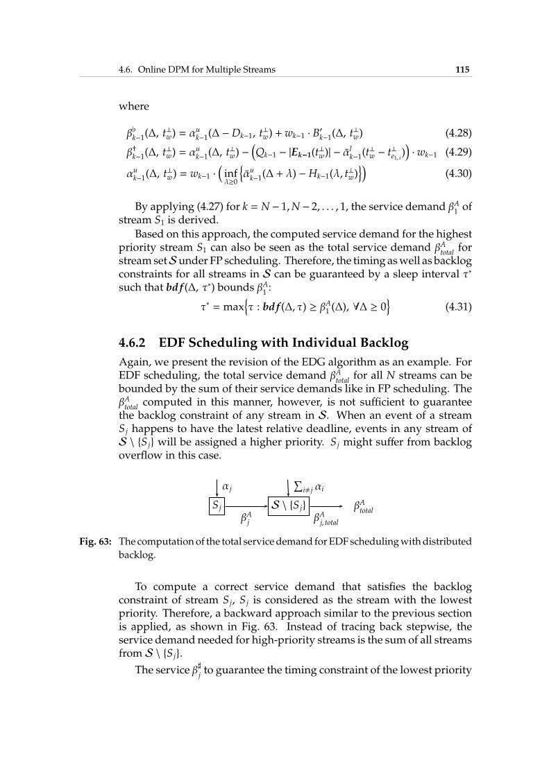
4.6. Online DPM for Multiple Streams 115
where
β♭k−1(∆, t⊥w) = α
uk−1(∆ −Dk−1, t
⊥w) + wk−1 · B
′k−1(∆, t
⊥w) (4.28)
β†k−1(∆, t⊥w) = α
uk−1(∆, t
⊥w) −(
Qk−1 − |Ek−1(t⊥w)| − α
lk−1(t
⊥w − t⊥e1, i)
)
· wk−1 (4.29)
αuk−1(∆, t⊥w) = wk−1 ·
(
infλ≥0
{
αuk−1(∆ + λ) −Hk−1(λ, t⊥w)})
(4.30)
By applying (4.27) for k = N − 1,N − 2, . . . , 1, the service demand βA1of
stream S1 is derived.
Based on this approach, the computed service demand for the highestpriority stream S1 can also be seen as the total service demand βA
totalfor
streamsetSunder FP scheduling. Therefore, the timing aswell as backlogconstraints for all streams in S can be guaranteed by a sleep interval τ∗
such that bdf (∆, τ∗) bounds βA1:
τ∗ = max{
τ : bdf (∆, τ) ≥ βA1 (∆), ∀∆ ≥ 0}
(4.31)
4.6.2 EDF Scheduling with Individual Backlog
Again, we present the revision of the EDG algorithm as an example. ForEDF scheduling, the total service demand βA
totalfor all N streams can be
bounded by the sum of their service demands like in FP scheduling. TheβAtotal
computed in this manner, however, is not sufficient to guaranteethe backlog constraint of any stream in S. When an event of a streamS j happens to have the latest relative deadline, events in any stream ofS \ {S j} will be assigned a higher priority. S j might suffer from backlogoverflow in this case.
S j S \ {S j} βAtotal
α j∑
i, j αi
βAj
βAj, total
Fig. 63: The computationof the total servicedemand forEDF schedulingwithdistributed
backlog.
To compute a correct service demand that satisfies the backlogconstraint of stream S j, S j is considered as the stream with the lowestpriority. Therefore, a backward approach similar to the previous sectionis applied, as shown in Fig. 63. Instead of tracing back stepwise, theservice demand needed for high-priority streams is the sum of all streamsfrom S \ {S j}.
The service β♯jto guarantee the timing constraint of the lowest priority
116 Chapter 4. Power Management
stream S j should be more than the demand βAjof S j, i.e.,
β♯j(∆) ≥ inf
{
β : βAj (∆, t⊥w) = sup
0≤λ≤∆
{β(λ) −N∑
i, j
αui (λ, t⊥w)}}
(4.32)
By inverting (4.32), we can derive β♯j(∆) as:
β♯j(∆) = βAj (∆ − λ, t
⊥w) +
N∑
i, j
αui (∆ − λ, t⊥w) (4.33)
where λ = sup{
τ : βAj(∆ − τ, t⊥w) = β
Aj(∆, t⊥w)
}
, and
βAj (∆, t⊥w) = max
{
β♭j(∆, t⊥w), β
†j (∆, t
⊥w), β
♯j(∆)}
(4.34)
where β♭jand β†
jare from (4.28) and (4.29). To guarantee the timing
constraint of all higher-priority streams, we also know that βAj,total
must be
no less than the demand of S \ {S j} as well. Therefore, we know that attime t⊥w,
βAj,total(∆) = max{
β♯j(∆),
N∑
i, j
β♭i (∆, t⊥w)}
(4.35)
Applying (4.35) to each steam inS, the service demand for each steamis computed. Because each stream could be the one with the lowestpriority in the worst case, only the maximum of them can be seen asthe total service demand for stream set S. Therefore, a feasible sleepinterval τ∗ that guarantees both deadline and backlog-size constraints canbe computed from the bounded delay function that bounds themaximumof individual streams:
τ∗ = max{
τ : bdf (∆, τ) ≥ maxi∈N{βAi,total(∆)}, ∀∆ ≥ 0
}
(4.36)
4.6.3 EDF Scheduling with Global Backlog
The approach to get the total service demand of S for global backlogis different from the approach for individual backlog. Without loss ofgenerality, we assume that a backlog with size Q is shared by all eventstreams in S.
For the HAD algorithm, because there is no backlog for eachevaluation, the relative deadline for each event ei, j in every stream Si
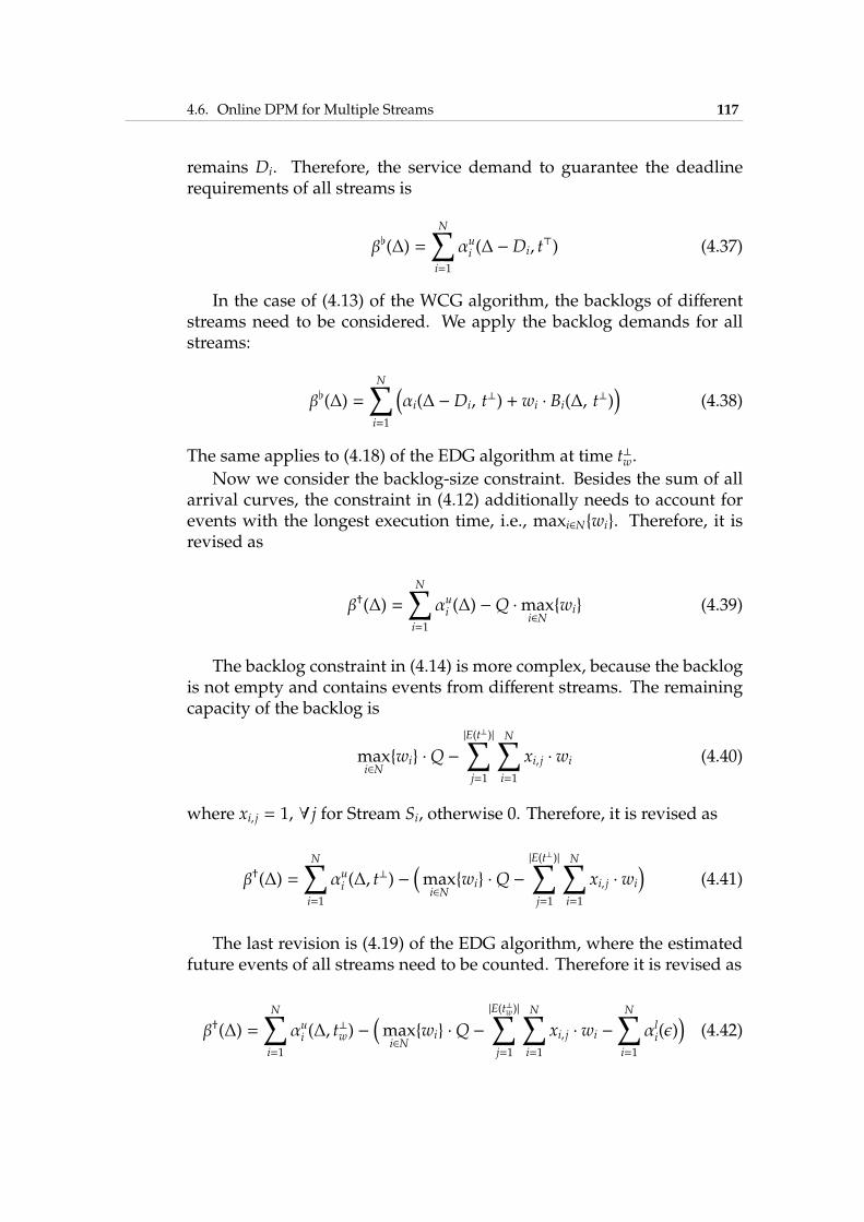
4.6. Online DPM for Multiple Streams 117
remains Di. Therefore, the service demand to guarantee the deadlinerequirements of all streams is
β♭(∆) =N∑
i=1
αui (∆ −Di, t⊤) (4.37)
In the case of (4.13) of the WCG algorithm, the backlogs of differentstreams need to be considered. We apply the backlog demands for allstreams:
β♭(∆) =N∑
i=1
(
αi(∆ −Di, t⊥) + wi · Bi(∆, t
⊥))
(4.38)
The same applies to (4.18) of the EDG algorithm at time t⊥w.
Now we consider the backlog-size constraint. Besides the sum of allarrival curves, the constraint in (4.12) additionally needs to account forevents with the longest execution time, i.e., maxi∈N{wi}. Therefore, it isrevised as
β†(∆) =N∑
i=1
αui (∆) −Q ·maxi∈N{wi} (4.39)
The backlog constraint in (4.14) is more complex, because the backlogis not empty and contains events from different streams. The remainingcapacity of the backlog is
maxi∈N{wi} ·Q −
|E(t⊥)|∑
j=1
N∑
i=1
xi, j · wi (4.40)
where xi, j = 1, ∀ j for Stream Si, otherwise 0. Therefore, it is revised as
β†(∆) =N∑
i=1
αui (∆, t⊥) −(
maxi∈N{wi} ·Q −
|E(t⊥)|∑
j=1
N∑
i=1
xi, j · wi
)
(4.41)
The last revision is (4.19) of the EDG algorithm, where the estimatedfuture events of all streams need to be counted. Therefore it is revised as
β†(∆) =N∑
i=1
αui (∆, t⊥w) −(
maxi∈N{wi} ·Q −
|E(t⊥w)|∑
j=1
N∑
i=1
xi, j · wi −
N∑
i=1
αli(ǫ))
(4.42)
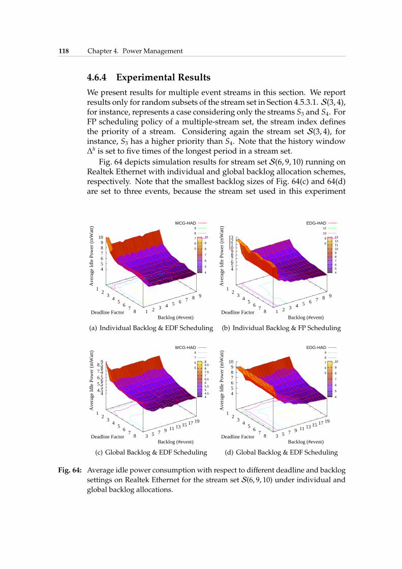
118 Chapter 4. Power Management
4.6.4 Experimental Results
We present results for multiple event streams in this section. We reportresults only for random subsets of the stream set in Section 4.5.3.1. S(3, 4),for instance, represents a case considering only the streams S3 and S4. ForFP scheduling policy of a multiple-stream set, the stream index definesthe priority of a stream. Considering again the stream set S(3, 4), forinstance, S3 has a higher priority than S4. Note that the history window∆h is set to five times of the longest period in a stream set.
Fig. 64 depicts simulation results for stream set S(6, 9, 10) running onRealtek Ethernet with individual and global backlog allocation schemes,respectively. Note that the smallest backlog sizes of Fig. 64(c) and 64(d)are set to three events, because the stream set used in this experiment
4
5
6
7
8
9
10
1 2
3 4
5 6
7 8 1 2 3 4 5 6 7 8 9
4 5 6 7 8 9
10
Ave
rage
Idl
e Po
wer
(m
Wat
t)
WCG-HAD 9
8
7
6
5
Deadline FactorBacklog (#event)
(a) Individual Backlog & EDF Scheduling
4 5 6 7 8 9 10 11 12 13
1 2
3 4
5 6
7 8 1 2 3 4 5 6 7 8 9
4 5 6 7 8 9
10 11 12 13
Ave
rage
Idl
e Po
wer
(m
Wat
t)EDG-HAD
12
10
8
6
Deadline FactorBacklog (#event)
(b) Individual Backlog & FP Scheduling
1 2
3 4
5 6
7 8 3 5 7 9 11 13 15 17 19
4 4.5
5 5.5
6 6.5
7 7.5
8 8.5
9
Ave
rage
Idl
e Po
wer
(m
Wat
t)
WCG-HAD 8
7
6
5
Deadline FactorBacklog (#event)
4 4.5 5 5.5 6 6.5 7 7.5 8 8.5 9
(c) Global Backlog & EDF Scheduling
1 2
3 4
5 6
7 8 3 5 7 9 11 13 15 17 19
4 5 6 7 8 9
10
Ave
rage
Idl
e Po
wer
(m
Wat
t)
EDG-HAD 9
8
7
6
5
Deadline FactorBacklog (#event)
4
5
6
7
8
9
10
(d) Global Backlog & EDF Scheduling
Fig. 64: Average idle power consumption with respect to different deadline and backlog
settings on Realtek Ethernet for the stream set S(6, 9, 10) under individual andglobal backlog allocations.
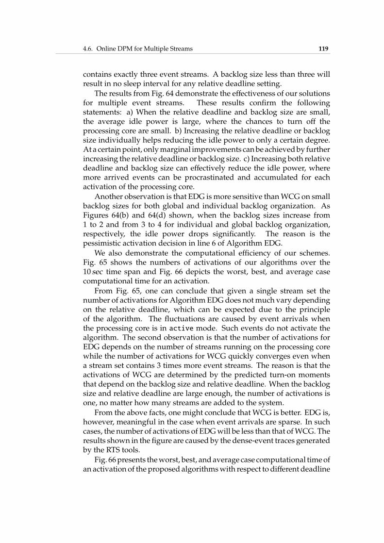
4.6. Online DPM for Multiple Streams 119
contains exactly three event streams. A backlog size less than three willresult in no sleep interval for any relative deadline setting.
The results from Fig. 64 demonstrate the effectiveness of our solutionsfor multiple event streams. These results confirm the followingstatements: a) When the relative deadline and backlog size are small,the average idle power is large, where the chances to turn off theprocessing core are small. b) Increasing the relative deadline or backlogsize individually helps reducing the idle power to only a certain degree.At a certainpoint, onlymarginal improvements canbeachievedby furtherincreasing the relative deadline or backlog size. c) Increasing both relativedeadline and backlog size can effectively reduce the idle power, wheremore arrived events can be procrastinated and accumulated for eachactivation of the processing core.
Another observation is that EDG ismore sensitive thanWCG on smallbacklog sizes for both global and individual backlog organization. AsFigures 64(b) and 64(d) shown, when the backlog sizes increase from1 to 2 and from 3 to 4 for individual and global backlog organization,respectively, the idle power drops significantly. The reason is thepessimistic activation decision in line 6 of Algorithm EDG.
We also demonstrate the computational efficiency of our schemes.Fig. 65 shows the numbers of activations of our algorithms over the10 sec time span and Fig. 66 depicts the worst, best, and average casecomputational time for an activation.
From Fig. 65, one can conclude that given a single stream set thenumber of activations for AlgorithmEDGdoes notmuch vary dependingon the relative deadline, which can be expected due to the principleof the algorithm. The fluctuations are caused by event arrivals whenthe processing core is in active mode. Such events do not activate thealgorithm. The second observation is that the number of activations forEDG depends on the number of streams running on the processing corewhile the number of activations for WCG quickly converges even whena stream set contains 3 times more event streams. The reason is that theactivations of WCG are determined by the predicted turn-on momentsthat depend on the backlog size and relative deadline. When the backlogsize and relative deadline are large enough, the number of activations isone, no matter how many streams are added to the system.
From the above facts, one might conclude that WCG is better. EDG is,however, meaningful in the case when event arrivals are sparse. In suchcases, the number of activations of EDGwill be less than that ofWCG. Theresults shown in the figure are caused by the dense-event traces generatedby the RTS tools.
Fig. 66presents theworst, best, andaverage case computational timeofan activation of the proposed algorithmswith respect to different deadline
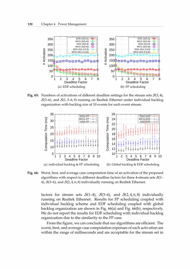
120 Chapter 4. Power Management
0
50
100
150
200
250
300
350
1 2 3 4 5 6 7 8
# A
ctiv
atio
n
Deadline Factor
EDG (S(3,4))WCG (S(3,4))EDG (S(3-6)
WCG (S(3-6))EDG (S(1,3-6,9)
WCG (S(1,3-6,9))
(a) EDF scheduling
0
50
100
150
200
250
300
350
1 2 3 4 5 6 7 8
# A
ctiv
atio
n
Deadline Factor
EDG (S(3,4))WCG (S(3,4))EDG (S(3-6)
WCG (S(3-6))EDG (S(1,3-6,9)
WCG (S(1,3-6,9))
(b) FP scheduling
Fig. 65: Numbers of activations of different deadline settings for the stream sets S(3, 4),S(3–6), and S(1, 3–6, 9) running on Realtek Ethernet under individual backlog
organization with backlog size of 10 events for each event stream.
5
10
15
20
25
30
35
1 2 3 4 5 6 7 8 9 10
Com
puta
tion
Tim
e (m
s)
Deadline Factor
EDG-FPWCG-FPHAD-FP
(a) individual backlog & FP scheduling
10
12
14
16
18
20
22
24
26
1 2 3 4 5 6 7 8 9 10
Com
puta
tion
Tim
e (m
s)
Deadline Factor
EDG-EDFWCG-EDFHAD-EDF
(b) Global backlog & EDF scheduling
Fig. 66: Worst, best, and average case computation time of an activation of the proposed
algorithms with respect to different deadline factors for three 4-stream sets S(1–
4), S(3–6), and S(2, 4, 6, 8) individually running on Realtek Ethernet.
factors for stream sets S(1–4), S(3–6), and S(2, 4, 6, 8) individuallyrunning on Realtek Ethernet. Results for FP scheduling coupled withindividual backlog scheme and EDF scheduling coupled with globalbacklog organization are shown in Fig. 66(a) and Fig. 66(b), respectively.We do not report the results for EDF scheduling with individual backlogorganization due to the similarity to the FP case.
From the figure, we can conclude that our algorithms are efficient. Theworst, best, and average case computation expenses of each activation arewithin the range of milliseconds and are acceptable for the stream set in
4.7. Offline Periodic DPM 121
Tab. 8. Specifically, the time to evaluate a decision is almost constanteven with large relative deadlines. In general, EDG is more expensivethan WCG and HAD, which can be expected from the definition inSection 4.5. The last observation is that the computation time is notnegligible. There are also means to tackle this problem, for instance,setting these computation overheads as a safe margin for the computedsleep period or making the activation itself the highest priority eventstream of the system.
4.7 Offline Periodic DPM
Distinct from the online adaptive algorithms in the previous sections, wepropose offline algorithms to derive optimal and approximated schemesfor periodic dynamic power management (PPM) in this section. Unlikethe online algorithms for which the activation/deactivation schedulingdecisions heavily depend on the complexity of the arrival curves, theoffline approaches off-load computation overhead to design time. Thelight run-time overhead of the periodic power management schemes isparticularly suitable for embedded systems that only have limited poweron computation. By simply using a hardware timer, an offline computedperiodic power management scheme can be applied to the processingcore. The control core is not necessary for the PPM in this section.
4.7.1 System Model and Problem Definition
Anabstractmodel of ourperiodic powermanagement (PPM) is illustratedin Fig. 67, inwhich powermanagement schemes are derived by analyzingthe arrival curves of event streamsS statically. Specifically, we first decidea period T = Ton + To f f , then switch the system to active/standbymodefor Ton time units, followed by To f f time units in sleepmode.
Based on model in Fig. 67, the energy consumption for a time intervalL, where L ≫ T and L
Tis an integer, consists of mode-switch overheads,
the energy in standby and sleep modes, and the energy for processingarrived events. Supposing that γi(L) is the number of events of eventstream Si served in interval L and all the served events finish in timeinterval L, the energy consumption E(L, Ton, To f f ) can be computed as
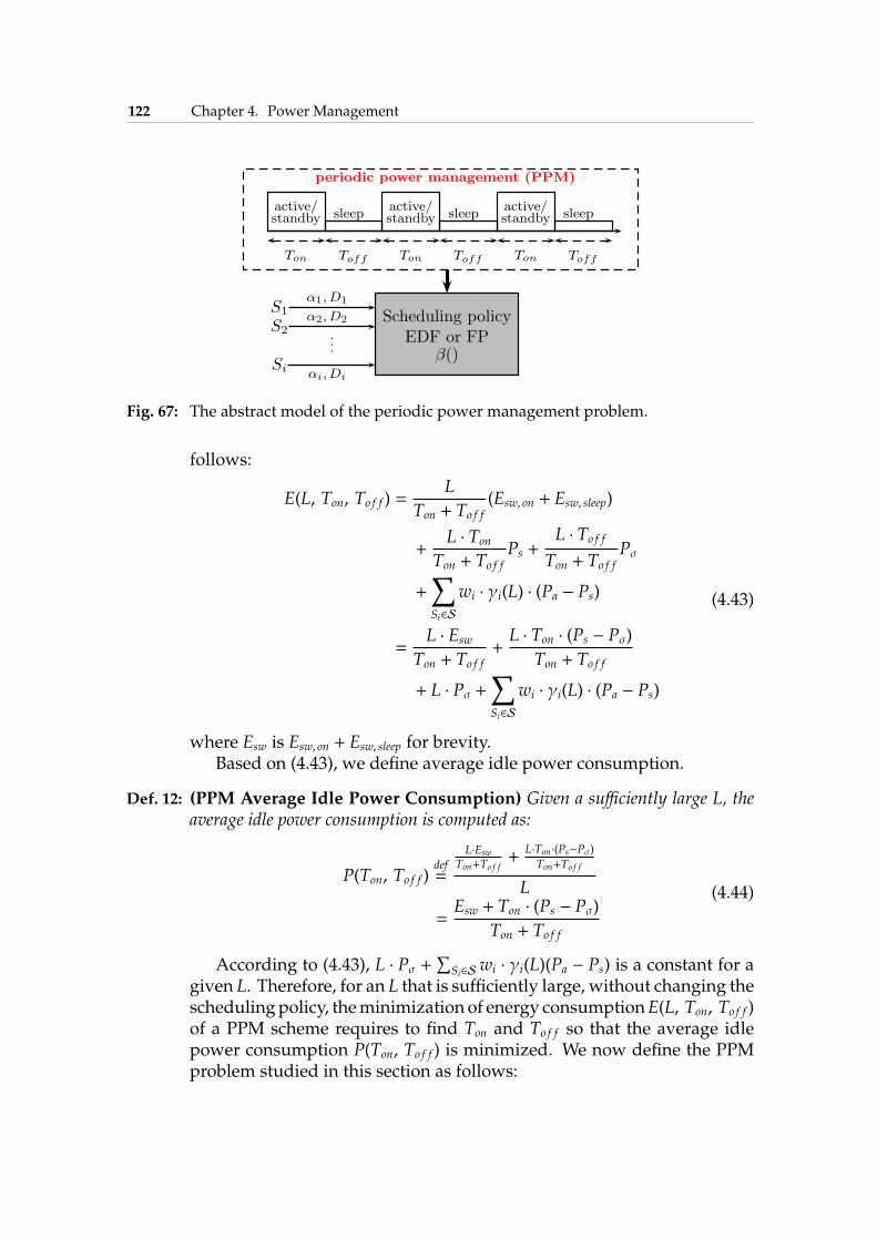
122 Chapter 4. Power Management
periodic power management (PPM)
Ton Toff Ton Toff Ton Toff
active/standby sleep
active/standby sleep
active/standby sleep
S1
S2
Si
α1, D1
α2, D2
...
αi, Di
Scheduling policyEDF or FP
β()
Fig. 67: The abstract model of the periodic power management problem.
follows:
E(L, Ton, To f f ) =L
Ton + To f f(Esw, on + Esw, sleep)
+L · Ton
Ton + To f fPs +
L · To f f
Ton + To f fPσ
+∑
Si∈S
wi · γi(L) · (Pa − Ps)
=L · Esw
Ton + To f f+L · Ton · (Ps − Pσ)
Ton + To f f
+ L · Pσ +∑
Si∈S
wi · γi(L) · (Pa − Ps)
(4.43)
where Esw is Esw, on + Esw, sleep for brevity.Based on (4.43), we define average idle power consumption.
Def. 12: (PPM Average Idle Power Consumption) Given a sufficiently large L, theaverage idle power consumption is computed as:
P(Ton, To f f )def=
L·Esw
Ton+To f f+
L·Ton·(Ps−Pσ)
Ton+To f f
L
=Esw + Ton · (Ps − Pσ)
Ton + To f f
(4.44)
According to (4.43), L · Pσ +∑
Si∈Swi · γi(L)(Pa − Ps) is a constant for a
given L. Therefore, for an L that is sufficiently large, without changing theschedulingpolicy, theminimization of energy consumptionE(L, Ton, To f f )of a PPM scheme requires to find Ton and To f f so that the average idlepower consumption P(Ton, To f f ) is minimized. We now define the PPMproblem studied in this section as follows:
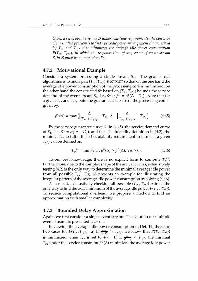
4.7. Offline Periodic DPM 123
Given a set of event streams S under real-time requirements, the objectiveof the studied problem is to find a periodic powermanagement characterizedby Ton and To f f that minimizes the average idle power consumptionP(Ton, To f f ), in which the response time of any event of event streamSi in S must be no more than Di.
4.7.2 Motivational Example
Consider a system processing a single stream S1. The goal of ouralgorithms is to find a pair (Ton,To f f ) ∈ R
+×R+ so that on the one hand theaverage idle power consumption of the processing core is minimized, onthe other hand the constructed βG based on (Ton,To f f ) bounds the servicedemand of the event stream S1, i.e., βG ≥ βA = αu1(∆ − D1). Note that fora given Ton and To f f pair, the guaranteed service of the processing core isgiven by:
βG(∆) = max(⌊ ∆
Ton + To f f
⌋
· Ton, ∆ −⌈ ∆
Ton + To f f
⌉
· To f f
)
(4.45)
By the service guarantee curve βG in (4.45), the service demand curveof S1, i.e., βA = αu1(∆ − D1), and the schedulability definition in (4.2), theminimal Ton to fulfill the schedulability requirement in terms of a givenTo f f can be defined as:
Tminon = min
{
Ton : βG(∆) ≥ βA(∆), ∀∆ ≥ 0
}
. (4.46)
To our best knowledge, there is no explicit form to compute Tminon .
Furthermore, due to the complex shape of the arrival curves, exhaustivelytesting (4.2) is the only way to determine the minimal average idle powerfrom all possible Ton. Fig. 68 presents an example for illustrating theirregular pattern of the average idle power consumption by solving (4.46).
As a result, exhaustively checking all possible (Ton, To f f ) pairs is theonlyway to find the exactminimumof the average idle powerP(Ton, To f f ).To reduce computational overhead, we propose a method to find anapproximation with smaller complexity.
4.7.3 Bounded Delay Approximation
Again, we first consider a single event stream. The solution for multipleevent streams is presented later on.
Reviewing the average idle power consumption in Def. 12, there aretwo cases for P(Ton,To f f ): a) If Esw
Ps−Pδ≥ To f f , we know that P(Ton,To f f )
is minimized when Ton is set to +∞. b) If Esw
Ps−Pδ< To f f , the minimal
Ton under the service constraint βG(∆) minimizes the average idle power
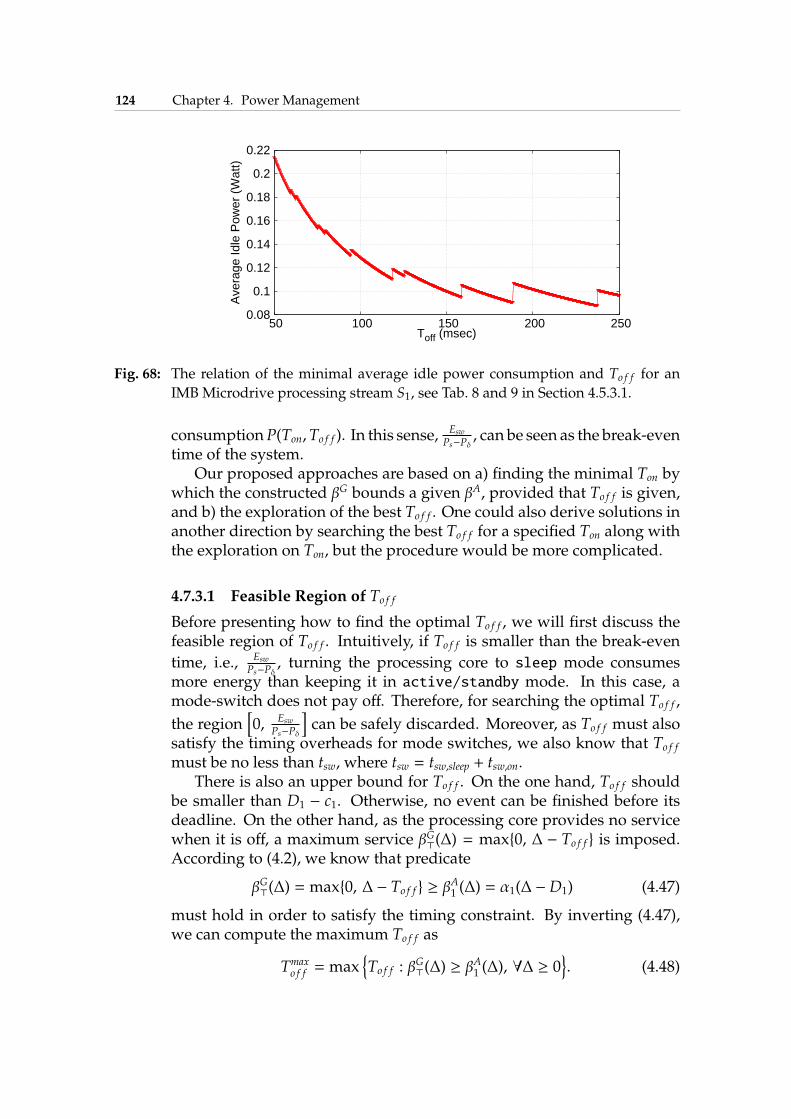
124 Chapter 4. Power Management
0.08
0.1
0.12
0.14
0.16
0.18
0.2
0.22
50 100 150 200 250
Ave
rage
Idle
Pow
er (
Wat
t)
Toff (msec)
Fig. 68: The relation of the minimal average idle power consumption and To f f for an
IMB Microdrive processing stream S1, see Tab. 8 and 9 in Section 4.5.3.1.
consumptionP(Ton,To f f ). In this sense, Esw
Ps−Pδ, can be seen as the break-even
time of the system.Our proposed approaches are based on a) finding the minimal Ton by
which the constructed βG bounds a given βA, provided that To f f is given,and b) the exploration of the best To f f . One could also derive solutions inanother direction by searching the best To f f for a specified Ton along withthe exploration on Ton, but the procedure would be more complicated.
4.7.3.1 Feasible Region of To f f
Before presenting how to find the optimal To f f , we will first discuss thefeasible region of To f f . Intuitively, if To f f is smaller than the break-even
time, i.e., Esw
Ps−Pδ, turning the processing core to sleep mode consumes
more energy than keeping it in active/standby mode. In this case, amode-switch does not pay off. Therefore, for searching the optimal To f f ,
the region[
0, Esw
Ps−Pδ
]
can be safely discarded. Moreover, as To f f must alsosatisfy the timing overheads for mode switches, we also know that To f f
must be no less than tsw, where tsw = tsw,sleep + tsw,on.There is also an upper bound for To f f . On the one hand, To f f should
be smaller than D1 − c1. Otherwise, no event can be finished before itsdeadline. On the other hand, as the processing core provides no servicewhen it is off, a maximum service βG⊤(∆) = max{0, ∆ − To f f } is imposed.According to (4.2), we know that predicate
βG⊤(∆) = max{0, ∆ − To f f } ≥ βA1 (∆) = α1(∆ −D1) (4.47)
must hold in order to satisfy the timing constraint. By inverting (4.47),we can compute the maximum To f f as
Tmaxo f f = max
{
To f f : βG⊤(∆) ≥ β
A1 (∆), ∀∆ ≥ 0
}
. (4.48)
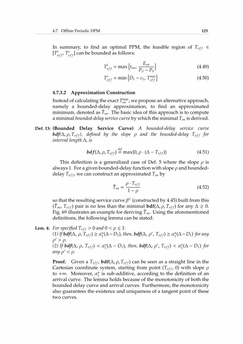
4.7. Offline Periodic DPM 125
In summary, to find an optimal PPM, the feasible region of To f f ∈
[Tlo f f, Tr
o f f] can be bounded as follows:
Tlo f f = max
{
tsw,Esw
PS − Pδ
}
(4.49)
Tro f f = min
{
D1 − c1, Tmaxo f f
}
(4.50)
4.7.3.2 Approximation Construction
Instead of calculating the exact Tminon , we propose an alternative approach,
namely a bounded-delay approximation, to find an approximatedminimum, denoted as Ton. The basic idea of this approach is to computea minimal bounded-delay service curve bywhich the minimal Ton is derived.
Def. 13: (Bounded Delay Service Curve) A bounded-delay service curvebdf(∆, ρ,To f f ), defined by the slope ρ and the bounded-delay To f f forinterval length ∆, is
bdf (∆, ρ,To f f )def= max{0, ρ · (∆ − To f f )} (4.51)
This definition is a generalized case of Def. 5 where the slope ρ isalways 1. For a given bounded-delay functionwith slope ρ and bounded-delay To f f , we can construct an approximated Ton by
Ton =ρ · To f f
1 − ρ(4.52)
so that the resulting service curve βG (constructed by 4.45) built from this(Ton, To f f ) pair is no less than the minimal bdf(∆, ρ,To f f ) for any ∆ ≥ 0.Fig. 69 illustrates an example for deriving Ton. Using the aforementioneddefinitions, the following lemma can be stated:
Lem. 4: For specified To f f > 0 and 0 < ρ ≤ 1:(1) If bdf(∆, ρ,To f f ) ≥ αu1(∆−D1), then, bdf(∆, ρ′, To f f ) ≥ αu1(∆−D1) for anyρ′ > ρ.(2) If bdf(∆, ρ, To f f ) < αu1(∆ − D1), then, bdf(∆, ρ′, To f f ) < αu1(∆ − D1) forany ρ′ < ρ.
Proof. Given a To f f , bdf(∆, ρ,To f f ) can be seen as a straight line in theCartesian coordinate system, starting from point (To f f , 0) with slope ρto +∞. Moreover, αu
1is sub-additive, according to the definition of an
arrival curve. The lemma holds because of the monotonicity of both thebounded delay curve and arrival curves. Furthermore, the monotonicityalso guarantees the existence and uniqueness of a tangent point of thesetwo curves.
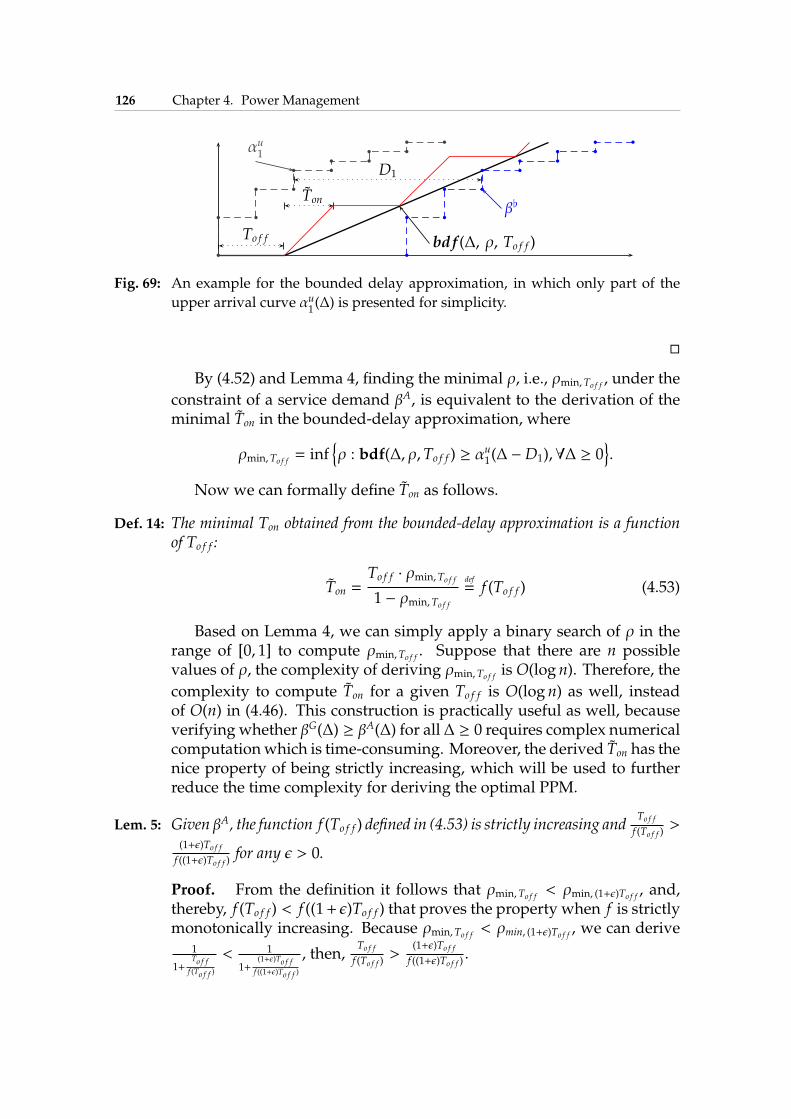
126 Chapter 4. Power Management
bdf (∆, ρ, To f f )
Ton
To f f
D1
αu1
β♭
b
b b
b b
b b
b b
b b
b b
b
b b
b b
b b
b b
b b
b b
Fig. 69: An example for the bounded delay approximation, in which only part of the
upper arrival curve αu1(∆) is presented for simplicity.
�
By (4.52) and Lemma 4, finding the minimal ρ, i.e., ρmin,To f f, under the
constraint of a service demand βA, is equivalent to the derivation of theminimal Ton in the bounded-delay approximation, where
ρmin,To f f= inf
{
ρ : bdf(∆, ρ,To f f ) ≥ αu1(∆ −D1),∀∆ ≥ 0
}
.
Now we can formally define Ton as follows.
Def. 14: The minimal Ton obtained from the bounded-delay approximation is a functionof To f f :
Ton =To f f · ρmin,To f f
1 − ρmin,To f f
def
= f (To f f ) (4.53)
Based on Lemma 4, we can simply apply a binary search of ρ in therange of [0, 1] to compute ρmin,To f f
. Suppose that there are n possiblevalues of ρ, the complexity of deriving ρmin,To f f
is O(log n). Therefore, the
complexity to compute Ton for a given To f f is O(logn) as well, insteadof O(n) in (4.46). This construction is practically useful as well, becauseverifying whether βG(∆) ≥ βA(∆) for all ∆ ≥ 0 requires complex numericalcomputationwhich is time-consuming. Moreover, the derived Ton has thenice property of being strictly increasing, which will be used to furtherreduce the time complexity for deriving the optimal PPM.
Lem. 5: Given βA, the function f (To f f ) defined in (4.53) is strictly increasing andTo f f
f (To f f )>
(1+ǫ)To f f
f ((1+ǫ)To f f )for any ǫ > 0.
Proof. From the definition it follows that ρmin,To f f< ρmin, (1+ǫ)To f f
, and,thereby, f (To f f ) < f ((1+ ǫ)To f f ) that proves the property when f is strictlymonotonically increasing. Because ρmin,To f f
< ρmin, (1+ǫ)To f f, we can derive
1
1+To f ff (To f f )
< 1
1+(1+ǫ)To f ff ((1+ǫ)To f f )
, then,To f f
f (To f f )>
(1+ǫ)To f f
f ((1+ǫ)To f f ).
4.7. Offline Periodic DPM 127
�
Based on the monotonicity of f (To f f ), we claim that the objectivefunction P(Ton, To f f ) obtained from the application of bounded-delayapproximated Ton defined in Def. 14 is convex.
Thm. 6: Using the bounded-delay algorithm approach to compute Ton = f (To f f ) asdepicted in (4.53), P(Ton, To f f ) = P( f (To f f ),To f f ) is a convex function.
Proof. The objective function P(Ton, To f f ) can be split into two parts:Esw
Ton+To f fand (Ps+Pδ) ·
Ton
Ton+To f f. For the first part Esw
Ton+To f f=
Esw
f (To f f )+To f f, f (To f f )+
To f f is strictly increasing according to Lemma 5. Therefore Esw
Ton+To f fis a
monotonically decreasing convex function. For the second part (Ps +
Pδ) ·Ton
Ton+To f f=
Ps+Pδ
1+To f ff (To f f )
, according to Lemma 5, we know that 1
1+To f ff (To f f )
is
monotonically increasing and is a convex function as well. As a linearcombination of convex functions is also a convex function, the originalfunction P(Ton, To f f ) is a convex function of To f f .
�
Thm. 6 allows to efficiently compute the optimal PPM, rather thanexhaustively searching for every possible To f f . The complexity, forinstance, is reduced to O(log n · logm) by applying a bisection search tothe feasible region of To f f . The pseudo code of the algorithm is describedin the Algorithm 6.
4.7.3.3 Optimal PPM
For comparison, we also present a brute-force algorithm, denoted as OPT,to find the minimal average idle power consumption P(Ton, To f f ), byexhaustively searching all possible (Ton, To f f ) pairs. The pseudo codeof OPT is depicted in Algorithm 7.
Due to the irregular shape of P(Ton, To f f ) as previously shown inFig. 68, OPT is the only way to find the exact optimum for our PPMproblem. Suppose that there are m possible To f f within the region[Tl
o f f, Tr
o f f], the complexity of OPT is thereby O(n ·m).
4.7.3.4 Multiple Streams Extension
When tacklingmultiple event streams, an essential problem is to computethe total service demand for a stream set S. The total service demand forS does not only depend on the service demand of individual streamsbut also the scheduling policy of the processing core. For fixed priority
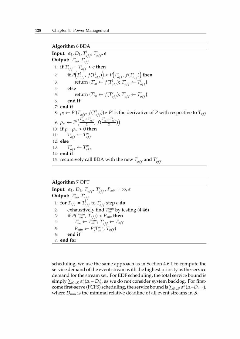
128 Chapter 4. Power Management
Algorithm 6 BDA
Input: α1, D1, Tlo f f
, Tro f f
, ǫOutput: T′on, T
′o f f
1: if Tro f f− Tl
o f f< ǫ then
2: if P(
Tlo f f, f (Tl
o f f))
< P(
Tro f f, f (Tr
o f f))
then
3: return {T′on ← f (Tlo f f
); T′o f f← Tl
o f f}
4: else5: return {T′on ← f (Tr
o f f); T′
o f f← Tr
o f f}
6: end if7: end if8: ρl ← P′(Tl
o f f, f (Tl
o f f)) ⊲ P′ is the derivative of Pwith respective to To f f
9: ρm ← P′(Tl
o f f+Tr
o f f
2, f (
Tlo f f+Tr
o f f
2))
10: if ρl · ρm > 0 then11: Tl
o f f← Tm
o f f
12: else13: Tr
o f f← Tm
o f f
14: end if15: recursively call BDA with the new Tl
o f fand Tr
o f f
Algorithm 7 OPT
Input: α1, D1, Tlo f f
, Tro f f
, Pmin = ∞, ǫOutput: T′on, T
′o f f
1: for To f f = Tlo f f
to Tro f f
step ǫ do
2: exhaustively find Tminon by testing (4.46)
3: if P(Tminon , To f f ) < Pmin then
4: T′on ← Tminon ; T′
o f f← To f f
5: Pmin ← P(Tminon , To f f )
6: end if7: end for
scheduling, we use the same approach as in Section 4.6.1 to compute theservice demand of the event streamwith the highest priority as the servicedemand for the stream set. For EDF scheduling, the total service bound issimply
∑
Si∈Sαui(∆ −Di), as we do not consider system backlog. For first-
comefirst-serve (FCFS) scheduling, the service bound is∑
Si∈Sαui(∆−Dmin),
where Dmin is the minimal relative deadline of all event streams in S.
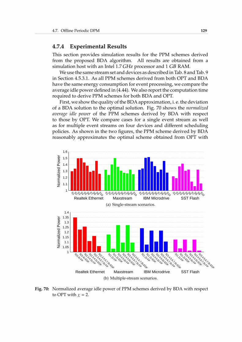
4.7. Offline Periodic DPM 129
4.7.4 Experimental Results
This section provides simulation results for the PPM schemes derivedfrom the proposed BDA algorithm. All results are obtained from asimulation host with an Intel 1.7GHz processor and 1 GB RAM.
Weuse the same streamset anddevices asdescribed inTab. 8 andTab. 9in Section 4.5.3.1. As all PPM schemes derived from both OPT and BDAhave the same energy consumption for event processing, we compare theaverage idle power defined in (4.44). We also report the computation timerequired to derive PPM schemes for both BDA and OPT.
First, we show the quality of theBDAapproximation, i. e. the deviationof a BDA solution to the optimal solution. Fig. 70 shows the normalizedaverage idle power of the PPM schemes derived by BDA with respectto those by OPT. We compare cases for a single event stream as wellas for multiple event streams on four devices and different schedulingpolicies. As shown in the two figures, the PPM scheme derived by BDAreasonably approximates the optimal scheme obtained from OPT with
1
1.1
1.2
1.3
1.4
1.5
1.6
S1 S2 S3 S4 S5 S6 S7 S8 S9 S10
S1 S2 S3 S4 S5 S6 S7 S8 S9 S10
S1 S2 S3 S4 S5 S6 S7 S8 S9 S10
S1 S2 S3 S4 S5 S6 S7 S8 S9 S10
Nor
mal
ized
Pow
er
SST FlashIBM MicrodriveMaxstreamRealtek Ethernet
(a) Single-stream scenarios.
1
1.05
1.1
1.15
1.2
1.25
1.3
1.35
1.4
S(3,4)-FP
S(3,4)-EDF
S(2,3,4,5)-FP
S(2,3,4,5)-EDF
S(2,3,4,5,7,9)-FP
S(2,3,4,5,7,9)-EDF
S(1,2)-FP
S(1,2)-EDF
S(3,4,5,6)-FP
S(3,4,5,6)-EDF
S(3,4,5,6,7,9)-FP
S(3,4,5,6,7,9)-EDF
S(1,2)-FP
S(1,2)-EDF
S(3,4,5,6)-FP
S(3,4,5,6)-EDF
S(3,4,5,6,7,9)-FP
S(3,4,5,6,7,9)-EDF
S(1,2)-FP
S(1,2)-EDF
S(3,4,5,6)-FP
S(3,4,5,6)-EDF
S(3,4,5,6,7,9)-FP
S(3,4,5,6,7,9)-EDF
Nor
mal
ized
Pow
er
SST FlashIBM MicrodriveMaxstreamRealtek Ethernet
(b) Multiple-stream scenarios.
Fig. 70: Normalized average idle power of PPM schemes derived by BDA with respect
to OPT with χ = 2.
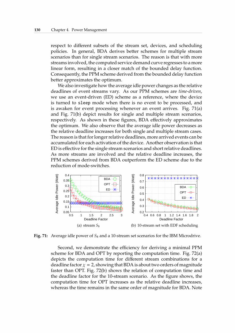
130 Chapter 4. Power Management
respect to different subsets of the stream set, devices, and schedulingpolicies. In general, BDA derives better schemes for multiple streamscenarios than for single stream scenarios. The reason is that with morestreams involved, the computed service demand curve regresses to amorelinear form, resulting in a closer match of the bounded delay function.Consequently, the PPM scheme derived from the bounded delay functionbetter approximates the optimum.
We also investigate how the average idle power changes as the relativedeadlines of event streams vary. As our PPM schemes are time-driven,we use an event-driven (ED) scheme as a reference, where the deviceis turned to sleep mode when there is no event to be processed, andis awaken for event processing whenever an event arrives. Fig. 71(a)and Fig. 71(b) depict results for single and multiple stream scenarios,respectively. As shown in these figures, BDA effectively approximatesthe optimum. We also observe that the average idle power decreases asthe relative deadline increases for both single and multiple stream cases.The reason is that for longer relative deadlines, more arrived events can beaccumulated for each activation of the device. Another observation is thatED is effective for the single stream scenarios and short relative deadlines.As more streams are involved and the relative deadline increases, thePPM schemes derived from BDA outperform the ED scheme due to thereduction of mode-switches.
0.05
0.1
0.15
0.2
0.25
0.3
0.35
0.4
0.5 1 1.5 2 2.5 3
Ave
rage
Idle
Pow
er (
Wat
t)
Deadline Factor
BDA
OPT
ED
(a) stream S8
0.2
0.3
0.4
0.5
0.6
0.7
0.8
0.4 0.6 0.8 1 1.2 1.4 1.6 1.8 2
Ave
rage
Idle
Pow
er (
Wat
t)
Deadline Factor
BDA
OPT
ED
(b) 10-stream set with EDF scheduling
Fig. 71: Average idle power of S8 and a 10-stream set scenarios for the IBM Microdrive.
Second, we demonstrate the efficiency for deriving a minimal PPMscheme for BDA and OPT by reporting the computation time. Fig. 72(a)depicts the computation time for different stream combinations for adeadline factorχ = 2, showing that BDA is about twoorders ofmagnitudefaster than OPT. Fig. 72(b) shows the relation of computation time andthe deadline factor for the 10-stream scenario. As the figure shows, thecomputation time for OPT increases as the relative deadline increases,whereas the time remains in the same order of magnitude for BDA. Note
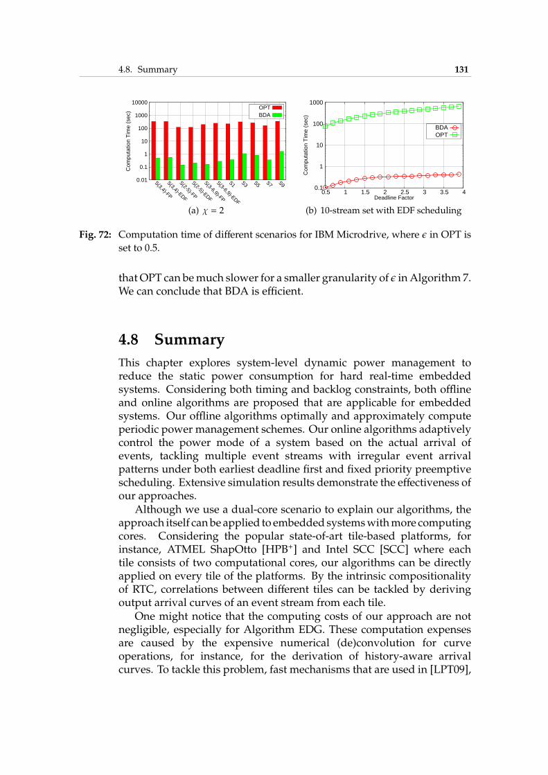
4.8. Summary 131
0.01
0.1
1
10
100
1000
10000
S(3,4)-FP
S(3,4)-EDF
S(2-5)-FP
S(2-5)-EDF
S(3-6,9)-FP
S(3-6,9)-EDF
S1 S3 S5 S7 S9
Com
puta
tion
Tim
e (s
ec)
OPTBDA
(a) χ = 2
0.1
1
10
100
1000
0.5 1 1.5 2 2.5 3 3.5 4
Com
puta
tion
Tim
e (s
ec)
Deadline Factor
BDAOPT
(b) 10-stream set with EDF scheduling
Fig. 72: Computation time of different scenarios for IBM Microdrive, where ǫ in OPT is
set to 0.5.
that OPT can bemuch slower for a smaller granularity of ǫ in Algorithm 7.We can conclude that BDA is efficient.
4.8 Summary
This chapter explores system-level dynamic power management toreduce the static power consumption for hard real-time embeddedsystems. Considering both timing and backlog constraints, both offlineand online algorithms are proposed that are applicable for embeddedsystems. Our offline algorithms optimally and approximately computeperiodic power management schemes. Our online algorithms adaptivelycontrol the power mode of a system based on the actual arrival ofevents, tackling multiple event streams with irregular event arrivalpatterns under both earliest deadline first and fixed priority preemptivescheduling. Extensive simulation results demonstrate the effectiveness ofour approaches.
Although we use a dual-core scenario to explain our algorithms, theapproach itself canbe applied to embedded systemswithmore computingcores. Considering the popular state-of-art tile-based platforms, forinstance, ATMEL ShapOtto [HPB+] and Intel SCC [SCC] where eachtile consists of two computational cores, our algorithms can be directlyapplied on every tile of the platforms. By the intrinsic compositionalityof RTC, correlations between different tiles can be tackled by derivingoutput arrival curves of an event stream from each tile.
One might notice that the computing costs of our approach are notnegligible, especially for Algorithm EDG. These computation expensesare caused by the expensive numerical (de)convolution for curveoperations, for instance, for the derivation of history-aware arrivalcurves. To tackle this problem, fast mechanisms that are used in [LPT09],
132 Chapter 4. Power Management
for instance, can be exploited to replace the expensive numericalcomputation.
5Conclusions
5.1 Main Results
The aim of this thesis is to address new challenges stemming from futuremany-core technologies for real-time embedded system. We categorizethe challenges into a few major topics and provide correspondingsolutions. The main contributions are summarized in the following:
• We present a programming model, which is suitable for streamingembedded systems. We adopt the Kahn process network forapplication modeling and design a hybrid programming syntax forthe specification of a target system. To assist the design ofmany-coreembedded systems, an iterator technique is developed by which aspecified system can be arbitrarily scaled in a parametrizedmanner.To avoid the costly communication and synchronization overheadincurred by large scale process networks, we propose a variation ofthe FIFO syntax ofKahnprocess network. Wealsodevelop aparallelfunctional simulation as a proof-of-concept runtime environmentfor this programming model. The presented results lead to the freeavailable software design toolchain in [dol].
• We investigate both analytic and simulation-based techniques forthe performance evaluation of multi/many-core embedded systemsat system level. For the analytic approach, we investigate modularperformance analysis basedon real-time calculus. We inspect timingcorrelations between data streams and present new methods toanalyze correlated data streams that originate from a same source.
134 Chapter 5. Conclusions
For simulation-basedmethod, we develop a trace-based frameworkwhich can estimate the performance of large-scale embeddedsystems with reasonable time as well as high accuracy. Both theanalytic method and the trace-based simulation can be served asa non-functional back-end for the aforementioned programmingmodel. They can be embedded into an automated design spaceexploration to assist the software design of embedded systems.
• we also investigate system-level power-efficient design in particularunder performance constraints. We propose offline and onlinealgorithms fordynamicpowermanagement, targeting the reductionof static power consumption under hard real-time constraints. Ouroffline algorithms compute periodic power management schemewhich switches the powermode of a systemby afixedperiodduringthe execution of the system. Alternatively, our online algorithmsadaptively control the powermode of a systemduring the executionof the system. We also develop methods to tackle multiple eventstreams under both preemptive earliest-deadline-first and fixed-priority scheduling policies.
5.2 Future Perspectives
The contributions presented in this thesis provide partial solutions for afew topics for future many-core real-time embedded systems. RevisitingFig. 2 in Section 1.3, more things deserve further investigation in order tocomplete the software design cycle. A few important future perspectivesare listed in the following:
• Themodernmulti-core and futuremany-core (often heterogeneous)architecture of embedded systems is characterized by a large designspace as there is a large degree of freedom in the partitioning ofparallel application tasks, the allocation of concurrent hardwarecomponents, their binding to application processes, and the choiceof appropriate resource allocation schemes. Because of theoverall system complexity, inspecting all design alternatives ofsuch a system, even analytically, is computationally prohibitive.Therefore, design space exploration techniques are critical tosupport important design decisions. The key for an efficient designspace exploration is efficient search methods. An efficient searchmethod requires not only fast convergence to the optimum but alsofair distribution of the search results in the case of multi-objectiveoptimization. To tackle this problem, evolutionary algorithmwouldbe a viable candidate as a starting point.
5.2. Future Perspectives 135
• The model-based design methodology opens a gap between thesystem-level specifications and the actual implementation of a sys-tem, sometimes referred to as the implementation gap [HHBT09a].Bringing this gap is challenging because on the one hand thesemantics of a model-of-computation has to be correctly preservedon the other hand desired performance of the complete HW/SWsystem has to be achieved. In the case of performance analysis atsystem level, this gap is also valid between the system specificationand the formal model of a system. Because the complexity ofmodern embedded systems increases, manually deriving the formalmodel of a system becomes error-prone. Therefore, an automatedsynthesis is desirable to close the gap.
• The energy issue is always valid. In this thesis, we consider only dy-namic power management to reduce the static power consumptionof a system. One interesting topic would be to combine dynamicpower management and dynamic voltage/frequency scaling toreduce both dynamic and static power consumption.
• Last but not least, an important topic is the thermal issue. Asmore computing cores are integrated into a single chip, the powerdensity of a chip is rapidly increased. The high temperature andheat generated by the high power density affect vital aspects of themulti/many-core embedded system pertaining to timing, reliability,fault-tolerance, and packaging and cooling costs. Therefore,thermal-aware design becomes crucial. A starting point at thisdirection could be to apply the techniques in Chapter 4 to considerthermal issue.

136 Chapter 5. Conclusions
Bibliography
[AAB+00] B. Ackland, A. Anesko, D. Brinthaupt, S.J. Daubert,A. Kalavade, J. Knobloch, E. Micca, M. Moturi, C.J.Nicol, J.H. O’Neill, J. Othmer, E. Sackinger, K.J. Singh,J. Sweet, C.J. Terman, and J. Williams. A single-chip, 1.6-billion, 16-b mac/s multiprocessor dsp. IEEEJournal of Solid-State Circuits, 35(3):412–424, March2000.
[ABM+04] Todd Austin, David Blaauw, Scott Mahlke, TrevorMudge, ChaitaliChakrabarti, andWayneWolf. Mobilesupercomputers. IEEE Computer, 37:81–83, 2004.
[AFM+02] T. Amnell, E. Fersman, L.Mokrushin, P. Petterson, andW. Yi. Times - a tool for medlling and implementationof embedded systems. In Proceedings of the 8thInternational Conference on Tools and Algorithms for theConstruction and Analysis of Systems (TACAS), pages460–464, 2002.
[AIS04] John Augustine, Sandy Irani, and Chaitanya Swamy.Optimal power-down strategies. In 45th Symposium onFoundations of Computer Science (FOCS), pages 530–539,October 2004.
[ati] Ati steam computing–technical overview.http://developer.amd.com/gpu_assets/Stream_Comp
uting_Overview.pdf.
[Bac77] John Backus. Can programming be liberated from thevon neumann style?: a functional style and its algebraof programs. ACM Turing award lectures, 1977.
[Bap06] Philippe Baptiste. Scheduling unit tasks to minimizethe number of idle periods: A polynomial timealgorithm for offline dynamic power management. In
138 Bibliography
Proceedings of the 17th annual ACM-SIAM symposium onDiscrete algorithm (SODA), pages 364–367, 2006.
[BDM09] G. Blake, R.G. Dreslinski, and T. Mudge. A survey ofmulticore processors. IEEE Signal ProcessingMagazine,26(6):26–37, November 2009.
[BFH+04] Ian Buck, Tim Foley, Daniel Horn, Jeremy Sugerman,Kayvon Fatahalian,MikeHouston, andPatHanrahan.Brook for gpus: stream computing on graphicshardware. In ACM SIGGRAPH, pages 777–786, NewYork, NY, USA, 2004. ACM.
[BFSS00] C. Brandolese, W. Fornaciari, F. Salice, andD. Sciuto. An instruction-level functionally-basedenergy estimation model for 32-bits microprocessors.In Proceedings of the 37th Annual Design AutomationConference (DAC), pages 346–351, 2000.
[Bor07] Shekhar Borkar. Thousand core chips: a technologyperspective. In Proceedings of the 44th annual DesignAutomation Conference (DAC), pages 746–749, NewYork, NY, USA, 2007. ACM.
[BTM00] D. Brooks, V. Tiwari, and M. Martonosi. Wattch: aframework for architectural-level power analysis andoptimizations. In Proceedings of the 27th InternationalSymposiumonComputerArchitecture, pages 83–94, 2000.
[Buc94] J.T. Buck. Static scheduling and code generation fromdynamic dataflow graphs with integer-valued controlstreams. In Conference Record of the Twenty-EighthAsilomar Conference on Signals, Systems and Computers,volume 1, pages 508–513, 1994.
[BWH+03] Felice Balarin, Yosinori Watanabe, Harry Hsieh,Luciano Lavagno, Claudio Passerone, and AlbertoSangiovanni-Vincentelli. Metropolis: An IntegratedElectronic System Design Environment. Computer,36(4):45–52, April 2003.
[BZCJ02] Amer Baghdadi, Nacer-Eddine Zergainoh, Wander O.Cesário, and Ahmed Amine Jerraya. Combin-ing a Performance Estimation Methodology witha Hardware/Software Codesign Flow Supporting
Bibliography 139
Multiprocessor Systems. IEEE Trans. on SoftwareEngineering, 28(9):822–831, 2002.
[CCBB09] Y.-K. Chen, C. Chakrabarti, S. Bhattacharyya, andB. Bougard. Signal processing on platformswith multiple cores: Part 1 - overview andmethodologies. IEEE Signal Processing Magazine,26(6):24–25, November 2009.
[CCS+08] J. Ceng, J. Castrillon, W. Sheng, H. Scharwachter,R. Leupers, G. Ascheid, H. Meyr, T. Isshiki, andH. Kunieda. Maps: An integrated framework formpsoc application parallelization. In Proceedings of the45th ACM/IEEE Design Automation Conference(DAC),pages 754–759, June 2008.
[CCZ06] B. Chopard, P. Combes, and J. Zory. A conservativeapproach to systemc parallelization. In InternationalConference on Computational Science (ICCS) Part IV,pages 653–660, 2006.
[CG06] Hui Cheng and Steve Goddard. Online energy-awareI/O device scheduling for hard real-time systems. InProceedings of the 9th Design, Automation and Test inEurope (DATE), pages 1055–1060, 2006.
[CK07] Jian-Jia Chen and Tei-Wei Kuo. Procrastinationdetermination for periodic real-time tasks in leakage-aware dynamic voltage scaling systems. In Int’l Conf.on Computer-Aided Design (ICCAD), pages 289–294,2007.
[CKT03] S. Chakraborty, S. Künzli, and L. Thiele. Ageneral framework for analysing system properties inplatform-based embedded systemdesigns. InProc. 6thDesign, Automation and Test in Europe (DATE), pages190–195, March 2003.
[CoW] CoWare Virtual Platform Analyzer.http://www.coware.com.
[Cri] Criticalblue multicore cascade.http://www.criticalblue.com/criticalblue_products/
multicore.html.
140 Bibliography
[Cru91a] R.L. Cruz. A calculus for network delay. IEEE Trans.Information Theory, 37(1):114–141, 1991.
[Cru91b] R.L. Cruz. A calculus for network delay. I. networkelements in isolation. IEEE Transactions on InformationTheory, 37(1):114–131, Jan 1991.
[CST09] Jian-Jia Chen, Nikolay Stoimenov, and Lothar Thiele.Feasibility analysis of on-line dvs algorithms forscheduling arbitrary event streams. In Proceedingsof the 30th IEEE Real-Time Systems Symposium (RTSS),2009.
[CUD] nvidia cuda.http://www.nvidia.com/cuda.
[DA08] Vinay Devadas and Hakan Aydin. On the interplayof dynamic voltage scaling and dynamic powermanagement in real-time embedded applications.In Proceedings of ACM International Conference onEmbedded software (EMSOFT), pages 99–108, 2008.
[DA10] Vinay Devadas and Hakan Aydin. DFR-EDF: Aunified energy management framework for real-timesystems. IEEE Real-Time and Embedded Technology andApplications Symposium (RTAS), pages 121–130, 2010.
[dol] Distributed Operation Layer.http://www.tik.ee.ethz.ch/∼shapes.
[EDK] Xilinx Platform Studio and the Embedded Develop-ment Kit, EDK version 7.1i edition.http://www.xilinx.com/ise/.
[ELLSV97] Stephan Edwards, Luciano Lavagno, Edward A.Lee, and Alberto Sangiovanni-Vincentelli. Design ofEmbedded Systems: Formal Models, Validation, andSynthesis. Proceedings of the IEEE, 85(3):366–390,March1997.
[ET06] Stephan A. Edwards and Olivier Tardieu. SHIM: ADeterministic Model for Heterogeneous EmbeddedSystems. IEEE Trans. VLSI Syst., 14(8):854–867, August2006.
Bibliography 141
[FFS01] Alessandro Fin, Franco Fummi, and Denis Signoretto.The use of SystemC for design verification andintegration test of IP-cores. In Proceedings of the 14thAnnual IEEE International ASIC/SoC Conference, pages76–80, September 2001.
[FSSZ01] William Fornaciari, Donatella Sciuto, Cristina Silvano,and Vittorio Zaccaria. A Design Framework toEfficiently Explore Energy-Delay Tradeoffs. In Proc.of the international symposium on Hardware/softwarecodesign (CODES), pages 260–265, 2001.
[GB03] Marc Geilen and Twan Basten. Requirements on theexecution of Kahn process networks. In Proceedings ofthe 12th European conference on Programming (ESOP),pages 319–334, Berlin, Heidelberg, 2003. Springer-Verlag.
[GH99] B. Gennart and R. Hersch. Computer-aided synthesisof parallel image processing applications. InProceedings Conf. Parallel and Distributed Methods forImage Processing III, SPIE Int. Symp. on Opt. Science,Denver, SPIE Vol-3817, 48-61, 1999.
[GHF+06] Michael Gschwind, H. Peter Hofstee, Brian Flachs,Martin Hopkins, Yukio Watanabe, and TakeshiYamazaki. Synergistic processing in cell’s multicorearchitecture. IEEE Micro, 26:10–24, 2006.
[GHGGPGDM01] Michael González Harbour, José Javier Gutiérrez Gar-cía, José Carlos Palencia Gutiérrez, and José MaríaDrake Moyano. MAST: Modeling and AnalysisSuite for Real Time Applications. In Proc. EuromicroConference on Real-Time Systems, pages 125–134, Delft,The Netherlands, June 2001.
[GHV99] Tony D. Givargis, Henkel Henkel, and Frank Vahid.Interface andCachePowerExploration forCore-BasedEmbedded System Design. In Proc. of the IEEE/ACMint’l conf. on Computer-Aided Design (ICCAD), page 270,1999.
[GP09] Xavier Guerin and Frédéric Petrot. A system frame-work for the design of embedded software targetingheterogeneous multi-core socs. In Proceedings of the

142 Bibliography
2009 20th IEEE International Conference on Application-specific Systems, Architectures and Processors (ASAP),pages 153–160, Washington, DC, USA, 2009. IEEEComputer Society.
[Gri04] Matthias Gries. Methods for evaluating and coveringthe design space during early design development.Journal of Integrated VLSI, 38(2):131–183, 2004.
[Grü06] David Grünert. Window based fifos for communi-cation in on-chip multiprocessor systems. Master’sthesis, ETH Zürich, Switzerland, 2006.
[Hai10] Wolfgang Haid. Design and Performance Analysis ofMultiprocessor Streaming Applications. PhD thesis, ETHZurich, 2010.
[HE05] ArneHamann andRolf Ernst. Tdma time slot and turnoptimization with evolutionary search techniques. InProceedings of the 8th Design, Automation and Test inEurope (DATE), pages 312–317, 2005.
[HHBT09a] Wolfgang Haid, Kai Huang, Iuliana Bacivarov, andLothar Thiele. Multiprocessor soc software designflows. IEEE Signal Processing Magazine, 26(6):64–71,2009.
[HHBT09b] Kai Huang, Wolfgang Haid, Iuliana Bacivarov, andLothar Thiele. CouplingMPARMwithDOL. TechnicalReport 314, D-ITET, TIK, ETH Zürich, Nov. 2009.
[HHLA07] Jin Heo, Dan Henriksson, Xue Liu, and TarekAbdelzaher. Integrating adaptive components: Anemerging challenge in performance-adaptive systemsand a server farm case-study. In Proceedings of the 28thIEEE Real-Time Systems Symposium (RTSS), pages 227–238, 2007.
[HKH+09] Wolfgang Haid, Matthias Keller, Kai Huang, IulianaBacivarov, and Lothar Thiele. Generation andcalibration of compositional performance analysismodels for multi-processor systems. In Proc. IntlConference on Systems, Architectures, Modeling andSimulation (SAMOS), pages 92–99, Samos, Greece,2009.
Bibliography 143
[HKL+07] Soonhoi Ha, Sungchan Kim, Choonseung Lee,Youngmin Yi, Seongnam Kwon, and Young-Pyo Joo.Peace: A hardware-software codesign environmentfor multimedia embedded systems. ACM Trans. Des.Autom. Electron. Syst., 12(3):1–25, 2007.
[HPB+] Wolfgang Haid, Pier Paolucci, Iuliana Bacivarov, KaiHuang, Francesco Simula, Piero Vicini, Xavier Guerin,Alexandre Chagoya-Garzon, Stefan Kraemer, andRainer Leupers. Shapes: A scalable HW/SW platformfor embedded systems. Unpublished.
[HSC+09] Kai Huang, Luca Santinelli, Jian-Jia Chen, LotharThiele, and Giorgio C. Buttazzo. Periodic powermanagement schemes for real-time event streams. Inthe 48th IEEEConf. onDecision andControl (CDC), pages6224–6231, Shanghai, China, 2009.
[HSH+09] Wolfgang Haid, Lars Schor, Kai Huang, IulianaBacivarov, and Lothar Thiele. Efficient execution ofkahn process networks on multi-processor systemsusing protothreads and windowed fifos. In Proc. IEEEWorkshop on Embedded Systems for Real-TimeMultimedia(ESTIMedia), pages 35–44, Grenoble, France, 2009.
[HT07] Wolfgang Haid and Lothar Thiele. Complex TaskActivation Schemes in System Level PerformanceAnalysis. In Proc. Int’l Conf. on Hardware/SoftwareCodesign and System Synthesis (CODES/ISSS), pages173–178, Salzburg, Austria, October 2007.
[Int] ISO/IEC 13818-2: Information technology — GenericCoding of moving pictures and associated audioinformation — Part 2: Video.
[ISG03] Sandy Irani, Sandeep Shukla, and Rajesh Gupta.Algorithms for power savings. InProceedings of the 14thAnnual ACM-SIAM Symposium on Discrete Algorithms(SODA), pages 37–46, 2003.
[ITR] International technology roadmap for semiconductors2007 edition: System drivers.http://www.itrs.net/Links/2007ITRS/2007_Chapters/
2007_SystemDrivers.pdf.
144 Bibliography
[Jai81] A.K. Jain. Image data compression: A review.Proceedings of the IEEE, 69(3):349–389, march 1981.
[JP08] F. Ryan Johnson and Joann M. Paul. InterruptModeling for Efficient High-Level Scheduler DesignSpace Exploration. ACM Trans. Des. Autom. Electron.Syst., 13(1):1–22, 2008.
[JPG04] R. Jejurikar, C. Pereira, and R. Gupta. Leakage awaredynamic voltage scaling for real-time embeddedsystems. In ACM/IEEE Design Automation Conference(DAC), pages 275–280, 2004.
[JRE04] M. Jersak, R.Henai, and R. Ernst. Context-awareperformance analysis for efficient embedded systemdesign. In Proc. Design, Automation and Test in Europe(DATE), March 2004.
[KAG+09] L.J. Karam, I. AlKamal, A. Gatherer, G.A. Frantz, D.V.Anderson, and B.L. Evans. Trends in multicore dspplatforms. IEEE Signal Processing Magazine, 26(6):38–49, November 2009.
[Kah74] Gilles Kahn. The Semantics of a Simple Language forParallel Programming. In Proceedings of IFIP Congress,North Holland Publishing Co, 1974.
[KB09] Hahn Kim and Robert Bond. Multicore softwaretechnologies. IEEE Signal Processing Magazine,26(6):80–89, November 2009.
[KBC09] BranislavKisacanin, Shuvra S. Bhattacharyya, and SekChai, editors. Embedded Computer Vision. SpringerLondon, 2009.
[KDVvdW97] Bart Kienhuis, Ed Deprettere, Kees Vissers, and Pietervan der Wolf. An Approach for Quantitative Analysisof Application-Specific Dataflow Architectures. InProceedings of the IEEE International Conference onApplication-Specific Systems, Architectures and Processors(ASAP), pages 338–349, July 1997.
[KKO+06] TeroKangas, Petri Kukkala, HeikkiOrsila, Erno Salmi-nen, Marko Hännikäinen, and Timo D. Hämäläinen.UML-Based Multiprocessor SoC Design Framework.ACM Transaction on Embedded Comp. Systems, 5(2):281–320, May 2006.
Bibliography 145
[KNRSV00] K. Keutzer, A.R. Newton, J.M. Rabaey, andA. Sangiovanni-Vincentelli. System-Level Design:Orthogonalization Of Concerns and Platform-BasedDesign. IEEETrans. Computer-AidedDesign of IntegratedCircuits and Systems, 19(12):1523–1543, Dec 2000.
[KPBT06] S. Künzli, F. Poletti, L. Benini, and L. Thiele.Combining simulation and formal methods forsystem-level performance analysis. In Proc. Design,Automation and Test in Europe (DATE), March 2006.
[Kü06] Simon Künzli. Efficient Design Space Exploration forEmbedded Systems. PhD thesis, ETH Zurich, 2006.
[LAB+04] Mirko Loghi, Federico Angiolini, Davide Bertozzi,Luca Benini, and Roberto Zafalon. Analyzing on-chip communication in a MPSoC environment. InProceedings of the Design, Automation and Test in EuropeConference and Exhibition Volume II (DATE), pages 752–757, 2004.
[LGS+95] C. Loiseaux, S. Graf, J. Sifakis, A. Bouajjani, andS. Bensalem. Property preserving abstractions for theverification of concurrent systems. Form.Methods Syst.Des., 6(1):11–44, 1995.
[LM87] Edward Ashford Lee and David G. Messerschmitt.Synchronous Data Flow. In Proceedings of the IEEE,volume 75, pages 1235–1245, January 1987.
[LN00] Edward A. Lee and Steve Neuendorffer. MoML: AModeling Markup Language in XML. Version 0.4.Technical Report UCB/ERL M00/12, University ofCalifornia at Berkeley, March 2000.
[LP95] Edward A. Lee and Thomas M. Parks. DataflowProcess Networks. Proceedings of the IEEE, 83(5):773–799, May 1995.
[LPT09] Kai Lampka, Simon Perathoner, and Lothar Thiele.Analytic real-time analysis and timed automata:A hybrid method for analyzing embedded real-time systems. In Proceedings of ACM internationalconference on Embedded software (EMSOFT), pages 107–116, Grenoble, France, 2009. ACM.
146 Bibliography
[LRD01] K. Lahiri, A. Raghunathan, and S. Dey. Systemlevel performance analysis for designing on-chipcommunication architectures. IEEE Transactionson Computer Aided-Design of Integrated Circuits andSystems, 20(6):768–783, 2001.
[LSV98] Edward A. Lee and Alberto Sangiovanni-Vincentelli.A Framework for ComparingModels of Computation.IEEE Transaction on Computer-Aided Design of IntegratedCircuits Systems, 17(12):1217–1229, December 1998.
[LT01] J.Y. Le Boudec and P. Thiran. Network Calculus - ATheory of Deterministic Queuing Systems for the Internet.LNCS 2050, Springer Verlag, 2001.
[MCT05] Alexander Maxiaguine, Samarjit Chakraborty, andLothar Thiele. DVS for buffer-constrained architec-tures with predictable QoS-energy tradeoffs. In theInternational Conference on Hardware-Software Codesignand System Synthesis (CODES+ISSS), pages 111–116,2005.
[MDC+05] Samy Meftali, Anouar Dziri, Luc Charest, PhilippeMarquet, and Jean-Luc Dekeyser. SOAP baseddistributed simulation environment for System-on-Chip (SoC) design. In Forum on Specification and DesignLanguages (FDL), December 2005.
[MJU+09] M. Mehrara, T. Jablin, D. Upton, D. August,K. Hazelwood, and S. Mahlke. Multicore compilationstrategies and challenges. IEEE Signal ProcessingMagazine, 26(6):55–63, November 2009.
[MKT04] Alexander Maxiaguine, Simon Künzli, and LotharThiele. Workload characterization model for taskswith variable execution demand. In Proceedings of the7th Design, Automation and Test in Europe (DATE), 2004.
[MLMK05] Makoto Murata, Dongwon Lee, Murali Mani, andKohsuke Kawaguchi. Taxonomy of xml schemalanguages using formal language theory. ACM Trans.Internet Technol., 5(4):660–704, 2005.
[mpe] Reference MPEG-2 Decoder.http://www.mpeg.org/MPEG/video/mssg-free-mpeg
-software.html.
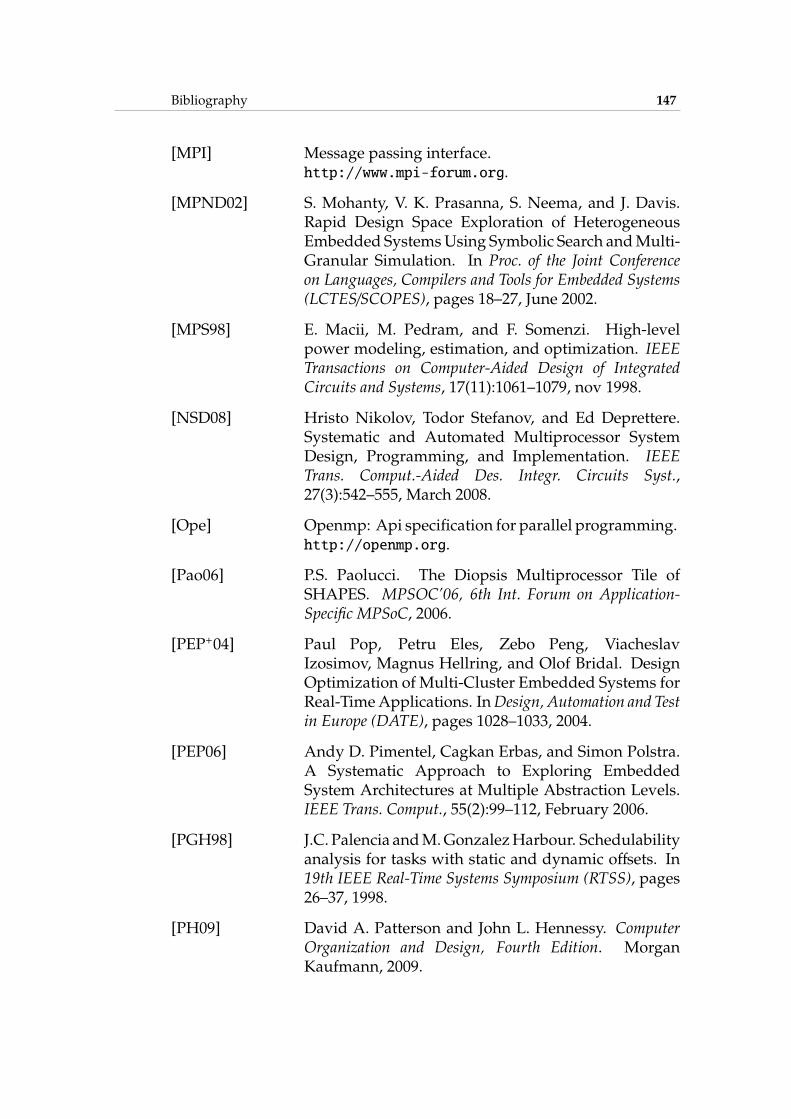
Bibliography 147
[MPI] Message passing interface.http://www.mpi-forum.org.
[MPND02] S. Mohanty, V. K. Prasanna, S. Neema, and J. Davis.Rapid Design Space Exploration of HeterogeneousEmbedded SystemsUsing Symbolic Search andMulti-Granular Simulation. In Proc. of the Joint Conferenceon Languages, Compilers and Tools for Embedded Systems(LCTES/SCOPES), pages 18–27, June 2002.
[MPS98] E. Macii, M. Pedram, and F. Somenzi. High-levelpower modeling, estimation, and optimization. IEEETransactions on Computer-Aided Design of IntegratedCircuits and Systems, 17(11):1061–1079, nov 1998.
[NSD08] Hristo Nikolov, Todor Stefanov, and Ed Deprettere.Systematic and Automated Multiprocessor SystemDesign, Programming, and Implementation. IEEETrans. Comput.-Aided Des. Integr. Circuits Syst.,27(3):542–555, March 2008.
[Ope] Openmp: Api specification for parallel programming.http://openmp.org.
[Pao06] P.S. Paolucci. The Diopsis Multiprocessor Tile ofSHAPES. MPSOC’06, 6th Int. Forum on Application-Specific MPSoC, 2006.
[PEP+04] Paul Pop, Petru Eles, Zebo Peng, ViacheslavIzosimov, Magnus Hellring, and Olof Bridal. DesignOptimization of Multi-Cluster Embedded Systems forReal-TimeApplications. InDesign, Automation and Testin Europe (DATE), pages 1028–1033, 2004.
[PEP06] Andy D. Pimentel, Cagkan Erbas, and Simon Polstra.A Systematic Approach to Exploring EmbeddedSystem Architectures at Multiple Abstraction Levels.IEEE Trans. Comput., 55(2):99–112, February 2006.
[PGH98] J.C. Palencia andM.GonzalezHarbour. Schedulabilityanalysis for tasks with static and dynamic offsets. In19th IEEE Real-Time Systems Symposium (RTSS), pages26–37, 1998.
[PH09] David A. Patterson and John L. Hennessy. ComputerOrganization and Design, Fourth Edition. MorganKaufmann, 2009.
148 Bibliography
[PHL+01] Andy D. Pimentel, Louis O. Hertzberger, PaulLieverse, Pieter van der Wolf, and Ed F. Deprettere.Exploring Embedded-Systems Architectures withArtemis. Computer, 34(11):57–63, 2001.
[pic] picochip pc205.http://www.picochip.com/page/76/Multi-core-PC205.
[PM93] W.B. Pennebacker and J.L. Mitchel. JPEG Still ImageData Compression Standard. Van Nostrand Reinhold,New York, 1993.
[PRT+10] Simon Perathoner, Tobias Rein, Lothar Thiele, KaiLampka, and Jonas Rox. Modeling structured eventstreams in system level performance analysis. InACMSIGPLAN/SIGBED Conference on Languages, Compilersand Tools for Embedded Systems (LCTES), pages 37–46,Stockholm, Sweden, 2010. ACM.
[PS05] H.D. Patel and S.K. Shukla. Towards a heterogeneoussimulation kernel for system-level models: a systemckernel for synchronous data flow models. IEEETransactions on Computer-Aided Design of IntegratedCircuits and Systems, 24(8):1261–1271, August 2005.
[pto] Ptolemy Project Home Page.http://ptolemy.eecs.berkeley.edu.
[RE02] K. Richter and R. Ernst. Event model interfaces forheterogeneous system analysis. In Proc. 5th Design,Automation and Test in Europe (DATE), pages 506–513,March 2002.
[RGB+08] Martino Ruggiero, Alessio Guerri, Davide Bertozzi,Michela Milano, and Luca Benini. A Fast andAccurate Technique for Mapping Parallel Applica-tions on Stream-Oriented MPSoC Platforms withCommunication Awareness. Int’l Journal of ParallelProgramming, 36(1):3–36, February 2008.
[RTE] RTEMS Steering Committee. RTEMS Home Page.
[SC05] Vishnu Swaminathan and Krishnendu Chakrabarty.Pruning-based, energy-optimal, deterministic I/Odevice scheduling for hard real-time systems. ACMTransactions in Embedded Computing Systems, 4(1):141–167, 2005.
Bibliography 149
[SCC] Single-chip cloud computer.http://techresearch.intel.com/articles/Tera-Scale/
1826.htm.
[SE09] Simon Schliecker and Rolf Ernst. A recursiveapproach to end-to-end path latency computation inheterogeneous multiprocessor systems. In Proc. 7thInternational Conference on Hardware Software Codesignand System Synthesis (CODES-ISSS), Grenoble, France,October 2009. ACM.
[SEDN05] Aviral Shrivastava, Eugene Earlie, Nikil Dutt, andAlex Nicolau. Aggregating processor free time for en-ergy reduction. In Proceedings of the 3rd IEEE/ACM/IFIPinternational conference on Hardware/software codesignand system synthesis (CODES+ISSS), pages 154–159,2005.
[SL04] Insik Shin and Insup Lee. Compositional Real-TimeScheduling Framework. In Proceedings of the Real-TimeSystems Symposium (RTSS), pages 57–67. IEEE Press,2004.
[Soc05] IEEE Computer Society. IEEE 1666 Standard SystemCLanguage Reference Manual.http://standards.ieee.org/getieee/1666/index.html,December 2005.
[SSG02] N. Savoiu, S.K. Shukla, and R.K. Gupta. Automatedconcurrency re-assignment in high level system mod-els for efficient system-level simulation. Proceedingsof Design, Automation and Test in Europe Conference andExhibition (DATE), pages 875–881, 2002.
[Ste04] Todor Stefanov. Converting weakly dynamic pro-grams to equivalent process network specifications,September 2004. Ph.D. dissertation book, LeidenUniversity, Leiden, The Netherlands, September 2004,ISBN: 90-9018629-8.
[sys] The Open SystemC Initiative (OSCI).http://www.systemc.org.
[SZT+04] T. Stefanov, C. Zissulescu, A. Turjan, B. Kienhuis,and E. Deprette. System design using khan processnetworks: the compaan/laura approach. InProceedings
150 Bibliography
of the Design, Automation and Test in Europe (DATE),pages 3400–345 Vol.1, February 2004.
[TBHH07] Lothar Thiele, Iuliana Bacivarov, Wolfgang Haid,and Kai Huang. Mapping applications to tiledmultiprocessor embedded systems. In Proc. 7th IntlConference on Application of Concurrency to SystemDesign (ACSD), pages 29–40, Bratislava, SlovakRepublic, 2007.
[TC94] Ken Tindell and John Clark. Holistic schedulabilityanalysis for distributed hard real-time systems.Microprocessing and Microprogramming, 40(2–3):117–134, 1994. Parallel Processing in Embedded Real-timeSystems.
[TCN00] Lothar Thiele, Samarjit Chakraborty, and MartinNaedele. Real-time calculus for scheduling hard real-time systems. In Proc. IEEE International Symposium onCircuits and Systems (ISCAS), volume 4, pages 101–104,2000.
[TI-] TI OMAP 4440.http://focus.ti.com/lit/ml/swpt034/swpt034.pdf.
[TIL] Tilera tile-gx100.http://www.tilera.com/products/TILE-Gx.php.
[TKA02] William Thies, Michal Karczmarek, and SamanAmarasinghe. StreamIt: A Language for StreamingApplications. In Proc. Int’l Conf. on CompilerConstruction, pages 179–196, Grenoble, France, April2002.
[Tra04] Mario Trams. Conservative distributed discrete eventsimulation with SystemC using explicit lookahead.http://digital-force.net/publications, 2004.
[TWS06] Lothar Thiele, Ernesto Wandeler, and NikolayStoimenov. Real-time interfaces for composing real-time systems. In International Conference On EmbeddedSoftware (EMSOFT), pages 34–43, 2006.
[VCC] The Cadence Virtual Component Co-design (VCC).http://www.cadence.com/products/vcc.html.
Bibliography 151
[vdWdKH+04] Pieter van der Wolf, Erwin de Kock, Tomas Hen-riksson, Wido Kruijtzer, and Gerben Essink. Designand Programming of Embedded Multiprocessors:An Interface-Centric Approach. In Proceedingsof the 2nd IEEE/ACM/IFIP international conferenceon Hardware/software codesign and system synthesis(CODES+ISSS), pages 206–217, Stockholm, Sweden,2004.
[vSP10] Peter van Stralen and Andy D. Pimentel. A high-levelmicroprocessor power modeling technique based onevent signatures. Journal of Signal Processing Systems,60(2):239–250, 2010.
[WHO06] T. Wild, A. Herkersdorf, and R. Ohlendorf. Perfor-mance Evaluation for System-on-Chip ArchitecturesUsing Trace-Based transaction fLevel Simulation. InProc. Design, Automation and Test in Europe (DATE),pages 248–253, 2006.
[WJM08] W. Wolf, A.A. Jerraya, and G. Martin. Multiprocessorsystem-on-chip (mpsoc) technology. IEEE Transactionson Computer-Aided Design of Integrated Circuits andSystems, 27(10):1701–1713, October 2008.
[wPOH09] Hae woo Park, Hyunok Oh, and Soonhoi Ha.Multiprocessor soc design methods and tools. IEEESignal Processing Magazine, 26(6):72–79, November2009.
[WT05] E. Wandeler and L. Thiele. Characterizing WorkloadCorrelations in Multi Processor Hard Real-Tim eSystems. In 11th IEEE Real-Time and EmbeddedTechnology and Applications Sympo sium (RTAS), pages46–55, March 2005.
[WT06a] Ernesto Wandeler and Lothar Thiele. Interface-Based Design of Real-Time Systems with HierarchicalScheduling. In Proc. Real-Time and Embedded TechnologyandApplications Symposium (RTAS), pages 243–252, SanJose, USA, 2006.
[WT06b] Ernesto Wandeler and Lothar Thiele. Optimal TDMATime Slot and Cycle Length Allocation for HardReal-Time Systems. In Proc. Asia and South Pacific
152 Bibliography
Conf. onDesignAutomation (ASP-DAC), pages 479–484,Yokohama, Japan, January 2006.
[WT06c] Ernesto Wandeler and Lothar Thiele. Real-TimeCalculus (RTC) Toolbox.http://www.mpa.ethz.ch/Rtctoolbox, 2006.
[WTVL06] Ernesto Wandeler, Lothar Thiele, Marcel Verhoef, andPaul Lieverse. System Architecture Evaluation UsingModular Performance Analysis: A Case Study. Int’lJournal on Software Tools for Technology Transfer (STTT),8(6):649–667, November 2006.
[YCHK07] Chuan-Yue Yang, Jian-Jia Chen, Chia-Mei Hung, andTei-Wei Kuo. System-level energy-efficiency for real-time tasks. In the 10th IEEE International SymposiumonObject/component/service-oriented Real-time distributedComputing (ISORC), pages 266–273, 2007.
[yel] Yellow Dog Linux.http://www.yellowdoglinux.com.
[YVKI00] W. Ye, N. Vijaykrishnan, M. Kandemir, andM.J. Irwin.The design and use of simplepower: a cycle-accurateenergy estimation tool. InProceedings of the 37thAnnualDesign Automation Conference (DAC), pages 340–345,2000.
[ZC05] Jianli Zhuo and Chaitali Chakrabarti. System-level energy-efficient dynamic task scheduling. InProceedings of the 42nd ACM/IEEE Design AutomationConference(DAC), pages 628–631, 2005.

List of Publications
The following list summarizes the publications on which this thesis arebased. The pertinent chapters of this thesis are given in brackets.
K. Huang, L. Santinelli, J. J. Chen, L. Thiele, and G. C. Buttazzo. AdaptiveDynamic Power Management for Hard Real-Time Streams. In Real-TimeSystems Journal (accepted)(Chapter 4)
K.Huang, L. Santinelli, J. J. Chen, L. Thiele, andG. C. Buttazzio. Adaptivepower management for real-time event streams. In the 15th IEEE Conf.on Asia and South Pacific Design Automation Conference (ASP-DAC), pages7–12, 2010.(Chapter 4)
K.Huang, L. Santinelli, J. J. Chen, L. Thiele, andG. C. Buttazzio. Adaptivedynamic power management for hard real-time systems. In the 30th IEEEReal-Time Systems Symposium (RTSS), pages 23–32, Washington D.C. U.S.,2009.(Chapter 4)
K. Huang, L. Santinelli, J.-J. Chen, L. Thiele, and G. C. Buttazzio. Periodicpowermanagement schemes for real-time event streams. In the 48th IEEEConf. on Decision and Control (CDC), pages 6224–6231, China, 2009.(Chapter 4)
K. Huang, I. Bacivarov, J. Liu, and W. Haid. A modular fast simulationframework for stream-oriented mpsoc. In IEEE Symposium on IndustrialEmbedded Systems (SIES), pages 74–81, Ecole Polytechnique Fédérale deLausanne, Switzerland, 2009.(Chapter 3)
K. Huang, L. Thiele, T. Stefanov, and E. Deprettere. Performanceanalysis of multimedia applications using correlated streams. In Design,Automation and Test in Europe (DATE), pages 912–917, Nice, France, 2007.(Chapter 3)
154 List of Publications
K.Huang, I. Bacivarov, F. Hugelshofer, and L. Thiele. Scalably distributedsystemc simulation for embedded applications. In IEEE Symposium onIndustrial Embedded Systems (SIES), pages 271–274, 2008.(Chapter 2)
K. Huang, D. Gruenert, and L. Thiele. Windowed fifos for fpga-based multiprocessor systems. In IEEE 18th International Conference onApplication-specific Systems, Architectures and Processors (ASAP), pages 36–42, Montreal, Canada, 2007.(Chapter 2)
L. Thiele, I. Bacivarov, W. Haid, and K. Huang. Mapping Applications toTiled Multiprocessor Embedded Systems. In Proceedings of InternationalConference on Application ofConcurrency to System Design (ACSD), pages29–40, Bratislava, Slovak Republic, July 2007.(Chapter 2)
It follows a list of publications that are not fully covered in this thesis.
K. Huang, W. Haid, I. Bacivarov, M. Keller and L. Thiele. Embeddingperformance analysis into the design cycle of mpsocs for real-timemultimedia. ACM Transactions on Embedded Computing Systems. (toappear)
J. J. Chen and K. Huang and L. Thiele Power Management Schemes forHeterogeneous Clusters under Quality of Service Requirements Streams26th ACM Symposium On Applied Computing (SAC) 2011
I. Bacivarov, W. Haid, K. Huang, and L. Thiele. Methods and Toolsfor Mapping Process Networks Onto Multi-Processor Systems. InBhattacharyya, Shuvra S. and Deprettere, Ed F. and Leupers, Rainer andTakala, Jarmo, editors Handbook of Signal Processing Systems. Springer,pages 1007—1040, Oct. 2010.
155
W. Haid, K. Huang, I. Bacivarov, and L. Thiele. Multiprocessor socsoftware design flows. IEEE Signal Processing Magazine, 26(6):64–71,2009.
W. Haid, L. Schor, Kai Huang, I. Bacivarov, and L. Thiele. Efficientexecution of kahn process networks on multi-processor systems usingprotothreads and windowed fifos. In Proc. IEEE Workshop on EmbeddedSystems for Real-Time Multimedia (ESTIMedia), pages 35–44, Grenoble,France, 2009.
K. Huang, W. Haid, I. Bacivarov, and L. Thiele. Coupling MPARM withDOL. Technical Report 314, D-ITET, TIK, ETH Zürich, Nov. 2009.
W. Haid, M. Keller, K. Huang, I. Bacivarov, and L. Thiele. Generationand calibration of compositional performance analysis models for multi-processor systems. In Proc. Intl Conference on Systems, Architectures,Modeling and Simulation (SAMOS), pages 92–99, Samos, Greece, 2009.
J. Liu, Z. h. Li, I. Bacivarov, and K. Huang. Scheduling mechanisms inhigh-level simulation framework. Microelectronics & Computer, 25(8):64–68, 2008.
T. Sporer, A. Franck, I. Bacivarov, M. Beckinger, W. Haid, K. Huang,L. Thiele, P. Paolucci, P. Bazzana, P. Vicini, J. J. Ceng, S. Kraemer, andR. Leupers. Shapes - a scalable parallel hw/sw architecture applied towave field synthesis. In Proc. 32nd Intl Audio Engineering Society (AES)Conference, pages 175–187, Hillerod, Denmark, 2007. Audio EngineeringSociety.
K. Huang, J. Gu, T. Stefanov, and E. Deprettere. Automatic PlatformSynthesis andApplicationMapping forMultiprocessor SystemsOn-Chip.Technical Report 05-30, LIACS, Leiden University, Aug. 2005.

156 Curriculum Vitae
Curriculum Vitae
Name Kai Huang
Date of Birth 2 October 1977
Nationality China
Website www.tik.ee.ethz.ch/∼khuang
Education:
10/2005–11/2010 ETH Zurich, Computer Engineering and Networks Labora-tory, SwitzerlandDoctor Thesis under the Supervision of Prof. Dr. Lothar Thiele
01/2004–08/2005 Leiden University, Leiden Institute of Advanced ComputerScience, the NetherlandsMaster of Computer Science
09/1995–06/1999 Fudan University, Dept. Computer Science, ChinaBachelor of Computer Science
Professional Experience:
10/2005–now Research & Teaching Assistant at ETH Zurich
10/2001–12/2003 Senior Software Engineer at Redsonic Inc, Shanghai, China
07/2001–10/2001 Program Analyzer at National Computer Systems Pte Ltd(NCS), Shanghai, China
07/1999–05/2001 Software Engineer at Fudan Network Ltd., Shanghai, China
Honors:
2010 Student Travel Grant for the 15th IEEE Conf. on Asia andSouth Pacific Design Automation Conference (ASP-DAC)
2009 General Chairs’ Recognition Award for Interactive Papers forthe 48th IEEE Conf. on Decision and Control (CDC)
2009 Co-recipient for the Best Paper Award Nomination for the7th IEEE Workshop on Embedded Systems for Real-TimeMultimedia (ESTIMedia)
2009 Co-recipient for the Best Paper Award for the Int’l Sympo-sium on Systems, Architectures, Modeling and Simulation(SAMOS)


![Soft Core] Soft-Core Processors for Embedded Systems](https://img.pdfslide.net/doc/110x75/577d25661a28ab4e1e9eb4a3/soft-core-soft-core-processors-for-embedded-systems.jpg)