Towards Statistical Modeling and Machine Learning Based

Towards Statistical Modeling and Machine Learning BasedEnergy Usage Forecasting in Smart Grid

Wei Yu∗, Dou An

§, David Griffith

†,Qingyu Yang

§, and Guobin Xu

∗

∗Towson University

Towson, MD [email protected]

[email protected]

§Xi’an Jiaotong UniversityXi’an, Shaanxi, China

[email protected]@mail.xjtu.edu.cn

†National Institute of

Standards and TechnologyGaithersburg, MD 20899

[email protected]

ABSTRACT

Developing effective energy resource management strategiesin the smart grid is challenging due to the entities on boththe demand and supply sides experiencing numerous fluctu-ations. In this paper, we address the issue of quantifyinguncertainties on the energy demand side. Specifically, wefirst develop approaches using statistical modeling analysisto derive a statistical distribution of energy usage. We thenutilize several machine learning based approaches such asthe Support Vector Machines (SVM) and neural networksto carry out accurate forecasting on energy usage. We per-form extensive experiments of our proposed approaches us-ing a real-world meter reading data set. Our experimentaldata shows that the statistical distribution of meter readingdata can be largely approximated with a Gaussian distribu-tion and the two SVM-based machine learning approachesto achieve a high accuracy of forecasting energy usage. Ex-tensions to other smart grid applications (e.g., forecastingenergy generation, determining optimal demand response,and anomaly detection of malicious energy usage) are dis-cussed as well.1

Categories and Subject Descriptors

C.4 [Performance of Systems]: Modeling Techniques

General Terms

Measurement, Performance

Keywords

Statistical Modeling Analysis, Energy Usage Forecasting,Machine Learning, Real-world Meter Reading Data, SmartGrid

1. INTRODUCTION

With recent developments in sensing, information, andcommunication technologies, the smart grid becomes a propos-ing system that makes the power grid more efficient, reliable,

1Copyright is held by the authors. This work isbased on an earlier work: RACS’14 Proceedings ofthe 2014 ACM Research in Adaptive and Conver-gent Systems, Copyright 2014 ACM 978-1-4503-3060-2.http://dx.doi.org/10.1145/2663761.2663768

and secure. To efficiently deliver energy resources in thesmart grid, an energy resource management strategy needsto be developed to balance the energy demand and supply[28]. Nonetheless, developing effective energy resource man-agement schemes is challenging due to the entities on boththe demand and supply sides experiencing numerous fluctu-ations. For example, on the supply side, fluctuations couldcome from distributed renewable energy resources due tosolar irradiance, wind speed, etc. On the demand side, nu-merous effects, including natural disasters, plug-in vehicles,personal habits of using energy, weather and temperature,etc., could make it difficult to predict energy usage.

To address these issues, in this paper, we develop tech-niques to effectively manage energy resources and usage inorder to adapt to fluctuations. Particularly, to balance en-ergy demand and supply, we develop effective techniques toaccurately model and forecast the amount of energy genera-tion and demand over time. Therefore, the issue of quantify-ing fluctuations on the energy demand side can be addressed.It is worth noting that the techniques developed in this papercan be applied to the energy generation side as well. We alsoconduct the modeling analysis to derive a statistical modelof energy usage and develop several machine learning basedapproaches to perform accurate forecasting of energy usage.The extensions to areas, including forecasting energy gener-ation, determining optimal demand response, and anomalydetection of malicious energy usage, are discussed as well.

To summarize, the key contributions of this paper are asfollows:

• First, using the real-world meter reading data set fromStanford University that consists of meter readingsfrom houses over 200 days2 as described in [18], westudy the statistical distribution of real-world meterreading data using non-parametric tests, including theShapiro-Wilk test [31] and the Quantile-Quantile plotnormality test [9]. The experimental data shows thatthe distribution of meter reading data can be approx-imated with a Gaussian distribution.

• Second, we develop machine learning based approachesto conduct accurate energy usage forecasting. Partic-

2The authors would like to acknowledge Mr. SebastienHoude at Stanford University for his dedicated help on pro-viding the real-world smart meter measurement data set.

APPLIED COMPUTING REVIEW MAR. 2015, VOL. 15, NO. 1 6

ularly, we consider the standard Radial Basis Func-tion (RBF) based SVM, the Least Squares (LS) basedSVM, and the Backward Propagation Neural Network(BPNN). In addition, we conduct extensive experi-ments using the aforementioned real-world meter read-ing data set to validate the effectiveness of these ap-proaches. The experimental data shows that the twoSVM-based approaches achieve a higher prediction ac-curacy than the BPNN based approach.

• Third, the techniques that we developed in this pa-per can be expanded to other areas as well, includ-ing the modeling and forecasting of energy generation,the optimal demand response, and anomaly detectionof malicious energy usage. Using the prediction ofwind speed as an example, the use of the SVM ma-chine learning based approach can be used to effec-tively conduct the forecasting on the distributed en-ergy resources in the energy supply side. In addition,the developed statistical modeling and forecasting re-sults can be applied to derive the upper and lowerbounds of energy usage and determine optimal demandresponse as well as anomaly detection of malicious en-ergy usage.

The remainder of this paper is organized as following: Theliterature review is conducted in Section 2. The problem ofbalancing the energy demand supply and the developed ap-proaches to perform the statistical modeling and forecastingof energy usage are presented in Section 3. The experi-mental results using real-world meter reading data set tovalidate the effectiveness of the developed approaches areshown in Section 4. The extensions of the work to otherareas (e.g., forecasting energy generation, determining opti-mal demand response, and performing anomaly detection ofmalicious energy usage) are presented in Section 5. Finally,the conclusion is drawn in Section 6.

2. RELATED WORK

A number of research efforts have been conducted to im-prove energy transmission and distribution efficiency [6, 10,25, 5, 20, 11]. For example, Guan et al. [10] proposed min-imizing the overall cost of electricity and natural gas for abuilding operation. Chen et al. [5] proposed an optimal de-mand response scheme that could match electricity supplyand shape electricity demand accordingly in both competi-tive and oligopolistic markets.

The challenges associated with the forecasting and de-mand response associated with energy usage were also dis-cussed in [23]. Broadly speaking, energy usage forecastingcan be categorized into short-term, medium-term, and long-term forecasting. For example, Hong et al. [13] adopted amultiple linear regression mechanism for conducting short-term forecasting, which provides an interpretability of thebehavior of the electricity usage in the service territory. Asemi-parametric additive model proposed by Fan et al. in[8] used a regression mechanism and investigated the nonlin-ear relationships between energy usage data and variables inthe short-term time period. In addition, a human-machineco-construct intelligence framework was proposed in [14] todetermine the horizon year load for a long term load fore-casting.

Machine learning methods such as SVM and neural net-works have been used in carrying out forecasting [2, 32, 37,35, 1, 19, 15, 29]. For example, Shi et al. [32] developed aSVM-based model for one-day-ahead power output forecast-ing using the characteristics of weather classification.

Different from the existing research efforts, using the real-world meter reading data set [18], non-parametric tests wereused to investigate the statistical distribution of energy us-age. To the best of our knowledge, our paper is one ofthe first to validate that the statistical distribution of me-ter reading data can be largely approximated with a Gaus-sian distribution. In addition, two SVM and neural networkbased approaches were used to systematically perform theenergy usage forecasting and the effectiveness of these ma-chine learning approaches was systematically evaluated andcompared. The findings from the paper can be extended toother areas, including the energy generation forecasting, theoptimal demand response, and anomaly detection of mali-cious energy usage.

3. OUR APPROACHES

In this section, we first present an overview of the problemand our proposed approaches. We then describe the real-world data set and develop the non-parametric test basedapproaches to carry out statistical modeling. Finally, wediscuss machine learning based approaches to perform en-ergy usage forecasting.

3.1 Overview

In the smart grid, the electric power from generators canbe delivered through the power grid to large geographicalareas. High efficiency in power production and energy uti-lization can be realized through monitoring and control ofpower transmission and distribution processes. How to man-age both bulk and distributed energy resources and the con-sumption levels of consumers to balance energy supply anddemand is important. Nonetheless, developing effective man-agement techniques to balance energy supply and demandis a challenging task because both sides experience variousfluctuations.

To address this issue, we developed a statistical analysisand model of energy usage in this paper. We also developedmachine learning based approaches to conduct accurate fore-casting of energy usage. For the statistical modeling, weuse two types of non-parametric test approaches to derivethe distribution of energy usage based on real-world meterreading data. For forecasting energy usage, we developedseveral machine learning based approaches to conduct ac-curate energy usage forecasting. Energy providers can usethese techniques to schedule energy generation and to makeenergy transmission and distribution efficient.

3.2 Real-world Energy Usage Data Set

We now introduce the real-world data set from StanfordUniversity, which consists of meter readings from houses over200 days (between February 2010 and October 2010) [18].In this data set, weather information (e.g., mean tempera-ture) for each 24 hour period is taken from archival data atWeather Underground website. We use meter readings andweather information for 283 houses in our experiments inSection 4.


An example of meter reading is shown in Table 1. Fromthe table, each house is assigned an ID. The meter readingdata for energy usage is measured hourly. The fields con-tained in the data set are shown in Table 2, which consists ofthe house ID , time, energy usage, the maximum, mean, andminimum value of temperature, and maximum and meanvalue of wind speeds. The house size (i.e., the area) is in-cluded as well. As an example, the information shown inTable 3 is the data associated with house 1001 that is fora rented townhouse, built in 2004, with 92.90 − 139.35 sq.meters. In Table 4, we show an example of meter readingsfor energy usage and weather information at 2 p.m. fromdays 100 to 102 for house 1001. On day 100, the energyusage is 2.20 kilowatt hours (KWh) and the mean values oftemperature and wind speed are 50 Fahrenheit degrees (F )and 20.92 Km Per Hour (KmPH), respectively.

Table 1. Data Range and Time Scale

Data Type Range

ID of Houses 1-283Time Interval Hourly

Time Span Approximately 200 daysNumber of Data Points Approximately 4800 (one per hour)

Table 2. Data Fields

Max Temp Mean Temp Min TempMax WindSpeed Mean WindSpeed ID

Day-of-Year Hour Electricity Consumption

Table 3. Sample of House Information

ID Building Rent Year Const. Size

1001Townhouse, duplex

or row houseRent 2004 92.90-139.35

sq. meters

1002Single Family

Detached HouseOwn 1992 185.81-232.37

sq. meters

3.3 Statistical Model of Energy Usage

To establish a statistical model of energy usage, we de-velop two non-parametric test based approaches to derivethe statistical distribution of energy usage based on theaforementioned real-world meter reading data. We use anon-parametric test to carry out the analysis of the energyusage data. For a set of one-dimensional data, commonnon-parametric test approaches include the Shapiro-Wilktest [31] and the Kolmogorov-Smirnov (K-S) test [12]. Itis worth noting that because the K-S test demands the pre-knowledge of the distribution of the sample data, the testresult will not be credible if the population’s CumulativeDistribution Function (CDF) is estimated from the sampledata. It is worth noting that the predetermined CDF of themeter data is not known, so we consider the Shapiro-Wilktest to test the distribution of the sample data. We also useanother non-parametric test approach, which is also calledQuantile-Quantile (Q-Q) plot normality test, to confirm thedistribution of meter reading data [36]. On the plot, whentwo data sets are identically distributed, the Q-Q plot willbe shown a line. Then, we know that the greater the depar-ture from the reference line, the greater the chance that thetwo data sets are drawn with different distributions.

Table 4. An Example of Real-World MeterReading Data

Day EU Max T Mean T Min T Max W Mean W

100 2.20 55 50 46 33.80 20.92

101 1.29 57 54 50 22.53 12.87102 1.58 59 54 50 22.53 11.27

1 T stands for temperature (Fahrenheit degree (F )), W stands for wind

speed (Km per hour (KmPH)), and EU stands for energy usage (kilo-watt hour (KWh))

3.4 Machine Learning Based Approaches forEnergy Usage Forecasting

To accurately forecast energy usage in the smart grid, weuse the following machine learning based approaches: neuralnetwork based machine learning, the standard SVM and theleast squares SVM.

3.4.1 Neural Network Based Machine Learning

There are a number of research efforts on neural networks[16, 17]. A classic example of one of these neural networksis the Backward Propagation (BP) neural network, whichconsists of three layers: input layer, hidden layer, and outputlayer. Note that the error between real value and estimatedvalue will be propagated backward from output layer to hid-den layer and from hidden layer to input layer. The errorof each layer can be re-estimated and the weights can beassigned correspondingly. Parameters for neural networksare set through a training process that use known data setsas input. After the training process, the trained model canthen be used to carry out forecasting.

3.4.2 Standard SVM and LS-SVM

The standard SVM was originally proposed by V. N. Vap-nik et al. [7]. Generally speaking, the SVM is one of thepopular methods to efficiently classify data and to build aclassifier, which can be further used to carry out forecasting.In SVM, the data and associated features can be treated asa point and vectors in multi-dimensional space. The basicprinciple of a standard SVM is to find a hyperplane, whichcould divide the points into different spaces. By doing so,we can classify data into different categories [27]. In orderto minimize the classification error, the proper hyperplaneneeds to be determined.

The least squares SVM that is also denoted as LS-SVM isan enhanced SVM [33]. In a LS-SVM, there are two majorenhancements in comparison with the standard SVM. First,the inequality constraints are substituted by equality con-straints. Second, the squared loss function is used in theobjective function [34]. In our experiment, we use the radialbasis function as the kernel function in LS-SVM due to itswide use.

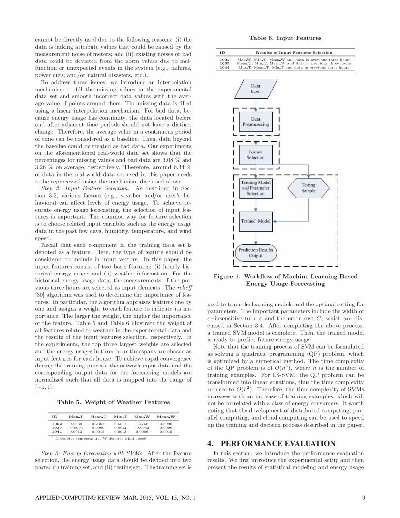
3.4.3 Workflow for Energy Usage Forecasting

As shown in Figure 1, the main process of machine learn-ing based approaches can be divided into the following threesteps: (i) data preprocessing, (ii) input feature selection, and(iii) energy usage forecasting. In the following, we describethese steps in detail.

Step 1: Data Preprocessing. To make our data more suit-able for energy forecasting, data preprocessing needs to per-formed first. Note that the real-world energy usage data


cannot be directly used due to the following reasons: (i) thedata is lacking attribute values that could be caused by themeasurement noise of meters; and (ii) existing noises or baddata could be deviated from the norm values due to mal-function or unexpected events in the system (e.g., failures,power cuts, and/or natural disasters, etc.).

To address these issues, we introduce an interpolationmechanism to fill the missing values in the experimentaldata set and smooth incorrect data values with the aver-age value of points around them. The missing data is filledusing a linear interpolation mechanism. For bad data, be-cause energy usage has continuity, the data located beforeand after adjacent time periods should not have a distinctchange. Therefore, the average value in a continuous periodof time can be considered as a baseline. Then, data beyondthe baseline could be treated as bad data. Our experimentson the aforementioned real-world data set shows that thepercentages for missing values and bad data are 3.08 % and3.26 % on average, respectively. Therefore, around 6.34 %of data in the real-world data set used in this paper needsto be reprocessed using the mechanism discussed above.

Step 2: Input Feature Selection. As described in Sec-tion 3.2, various factors (e.g., weather and/or user’s be-haviors) can affect levels of energy usage. To achieve ac-curate energy usage forecasting, the selection of input fea-tures is important. The common way for feature selectionis to choose related input variables such as the energy usagedata in the past few days, humidity, temperature, and windspeed.

Recall that each component in the training data set isdenoted as a feature. Here, the type of feature should beconsidered to include in input vectors. In this paper, theinput features consist of two basic features: (i) hourly his-torical energy usage, and (ii) weather information. For thehistorical energy usage data, the measurements of the pre-vious three hours are selected as input elements. The relieff[30] algorithm was used to determine the importance of fea-tures. In particular, the algorithm appraises features one byone and assigns a weight to each feature to indicate its im-portance. The larger the weight, the higher the importanceof the feature. Table 5 and Table 6 illustrate the weight ofall features related to weather in the experimental data andthe results of the input features selection, respectively. Inthe experiments, the top three largest weights are selectedand the energy usages in three hour timespans are chosen asinput features for each house. To achieve rapid convergenceduring the training process, the network input data and thecorresponding output data for the forecasting models arenormalized such that all data is mapped into the range of[−1, 1].

Table 5. Weight of Weather Features

ID Max T Mean T Min T Max W Mean W

1002 0.2539 0.2367 0.5011 1.4756 0.6090

1035 -0.0004 0.0060 0.0032 -0.0032 0.0090

1044 0.0013 0.0015 0.0013 0.0006 0.0019

1 T denotes temperature, W denotes wind speed

Step 3: Energy forecasting with SVMs. After the featureselection, the energy usage data should be divided into twoparts: (i) training set, and (ii) testing set. The training set is

Table 6. Input Features

ID Results of Input Features Selection

1002 Max W, Min T, Mean W and data in previous three hours1035 Mean T, Min T, Mean W and data in previous three hours

1044 Max T, Mean T, Min T and data in previous three hours

Figure 1. Workflow of Machine Learning BasedEnergy Usage Forecasting

used to train the learning models and the optimal setting forparameters. The important parameters include the width ofε−insensitive tube ε and the error cost C, which are dis-cussed in Section 3.4. After completing the above process,a trained SVM model is complete. Then, the trained modelis ready to predict future energy usage.

Note that the training process of SVM can be formulatedas solving a quadratic programming (QP) problem, whichis optimized by a numerical method. The time complexityof the QP problem is of O(n3), where n is the number oftraining examples. For LS-SVM, the QP problem can betransformed into linear equations, thus the time complexityreduces to O(n2). Therefore, the time complexity of SVMsincreases with an increase of training examples, which willnot be correlated with a class of energy consumers. It worthnoting that the development of distributed computing, par-allel computing, and cloud computing can be used to speedup the training and decision process described in the paper.

4. PERFORMANCE EVALUATION

In this section, we introduce the performance evaluationresults. We first introduce the experimental setup and thenpresent the results of statistical modeling and energy usage


forecasting.Based on the real-world meter reading data set described

in Section 3.2, we carried out extensive experiments to eval-uate the effectiveness of our developed statistical modelingand machine learning based energy usage forecasting ap-proaches. MATLAB R2010b3 was used to implement ourdeveloped approaches and the experiments were performedon a laptop PC (Centrino Duo, 2.3 GHz, 3 GB RAM). Thetoolkit LIBSVM in Matlab [4], a library for SVMs that in-cludes the implementation of both SVM and LS-SVM, wasused in our experiments. For comparison purposes, the neu-ral network toolbox in Matlab was also used to evaluate theperformance of the Backward Propagation (BP) neural net-work based forecasting approach, one of the classical neuralnetworks that consists of three layers: input layer, hiddenlayer, and output layer [17].

4.1 Results of Statistical Modeling

To perform the statistical modeling of energy usage, thetwo non-parametric test approaches: Shapiro-Wilk test andQ-Q plot normality test as we discussed in Section 3.3 areused. In our experiments, the meter reading measurementsover the following three time windows are aggregated: (i)morning (8:00-12:00), (ii) afternoon (14:00-18:00), and (iii)evening (20:00-24:00). Due to the space limitations, we onlyshow limited scenarios here using the energy usage measure-ments for house 1002, house 1035, and house 1044 as exam-ples. It is worth noting that two non-parametric tests on 200houses were performed at a significance level of α = 0.05.The experimental data shows that the meter readings of 148houses could be approximated by a Gaussian distribution.In addition, more than 40 % of the remaining 52 housescontain a number of 0 values and error information, whichlargely deviate from the normal values, leading to the fail-ures of the tests.

The Shapiro-Wilk test [31] with a significance level (α =0.05) is used for the measurements in individual time win-dows. It is worth noting that α is defined as the probabilitythat a Gaussian distribution approximation is mistakenlyrejected whereas it is actually true. Here, we consider twohypotheses: (i) H0: the data follows a Gaussian distribu-tion; and (ii) H1: the data does not follow a Gaussian dis-tribution. The P -value, in contrast to the threshold α, iscomputed based on the test statistics, which can be denotedas the probability, in the case of the null hypothesis H0, ofsampling results being equal to or being closer to the actualsampling results. As such, when the P -value is less than thepredetermined significance level α, the observed results arebe highly unlikely under the null hypothesis.

In our experiments, the P -value obtained from the me-ter reading measurements for the morning, afternoon, andevening windows are illustrated in Table 7. As shown in thetable, in addition to the P -value for the morning meter read-ing measurements at house 1002, the remaining P -values are

3Certain commercial equipment, instruments, or materialsare identified in this paper in order to specify the experimen-tal procedure adequately. Such identification is not intendedto imply recommendation or endorsement by the NationalInstitute of Standards and Technology (NIST), nor is it in-tended to imply that the materials or equipment identifiedare necessarily the best available for the purpose.

larger than the threshold of 0.05. Therefore, the energy us-age in morning, afternoon, and evening windows of thesehouses can be approximated with a Gaussian distribution.It is worth noting that the Shapiro-Wilk test on morningdata measurements from house 1002, in which the P -valueis 0.000813, is an example of a failure case. As the P -valueis far less than the threshold of 0.05, the morning data fromhouse 1002 cannot be approximated with a Gaussian distri-bution.

The Q-Q plot normality test [36] is also used to test thedistribution of meter reading measurements. As an exam-ple, the energy usage in house 1002 in three time windows isshown in Figure 2. The trend of points in Figures 2(b) and2(c) has a higher degree of approximation to a straight linethan the one in Figure 2(a), which indicates that the energyusages at noon and evening times can be better be approx-imated with the Gaussian distribution. This is because thecloser the points are to a line, the closer the reading is to aGaussian distribution. In Figure 2, there is significant devi-ation in the quantiles associated with the tails of the distri-bution whereas there is close agreement near the median. Tosummarize, the results of the two statistical test approachesdraw the same conclusion, that is, the meter reading mea-surements for the three time windows at the three housescan be approximated with a Gaussian distribution.

Table 7. Results of Shapiro-Wilk Test

ID Time Window P-value Hypothesis

Morning 0.000813 Reject

1002 Noon 0.3407 AcceptEvening 0.3236 Accept

Morning 0.08509 Accept1035 Noon 0.6062 Accept

Evening 0.526 Accept

Morning 0.4816 Accept1044 Noon 0.6121 Accept

Evening 0.6593 Accept

4.2 Results of Energy Usage Forecast

Experiments based on the real-world meter reading dataset used in this paper were conducted to validate the effec-tiveness of two types of SVM presented in Section 3 and BPneural network based approaches in terms of the accuracy ofenergy usage forecasting. In our experiments, based on themodels learned through the training process from the his-torical energy usage of the past 500 hours, we show the theaccuracy of energy usage forecasting in the next 48 hours.

To measure the accuracy of forecasting, the following threemetrics are considered: (i) MAPE (Mean Absolute Percent-age Error), (ii) MSE (Mean Square Error), and (iii) Co-efficient of Regression γ2, which are used to measure theerror between the actual and predicted energy usage. These

metrics are defined as follows: MAPE = 100n

∑ni=1

∣∣∣yi−yiyi

∣∣∣,

MSE = 1n

∑ni=1(yi − yi)

2, and γ2 =∑n

i (yi−y)2∑ni(yi−y)2

, where yi,

yi and y are actual value, forecasted value, and mean valueof the actual value, respectively.

We conducted a large number of experiments on meterreading data for 200 houses. Due to space limitations, onlya limited number of results are shown here for demonstrationpurposes. Based on the workflow showed in Section 3.4.3,the generic optimization mechanism provided by the LIB-


−2 −1 0 1 2

1.2

1.4

1.6

1.8

2.0

Theoretical Quantiles

Sam

ple

Qua

ntile

s

(a)

−2 −1 0 1 2

1.0

1.2

1.4

1.6

1.8

2.0

2.2


Sam

ple

Qua

ntile

s

(b)

−2 −1 0 1 2

0.5

1.0

1.5

2.0

2.5

3.0

3.5


Sam

ple

Qua

ntile

s

(c)

Figure 2. Q-Q Plot on No. 1002 House (a) Morning, (b) Noon, and (c) Evening

0 10 20 30 40 500.1

0.15

0.2

0.25

0.3

0.35

0.4

0.45

Hour

Energ

y C

onsu

mpti

on

Actual

Predict

(a)

0 10 20 30 40 50

0.2

0.25

0.3

0.35

0.4

0.45

0.5

Hour

Energ

y C

onsum

pti

on

Actual

Predict

(b)

0 100 200 300 400 5000.1

0.2

0.3

0.4

0.5Train Set Regression Predict by SVM

original

predict

0 10 20 30 40 500.2

0.25

0.3

0.35

0.4

Hour

Energ

y C

onsum

pti

on

Test Set Regression Predict by SVM

original

predict

(c)

Figure 3. Forecasting Accuracy of (a) BPNN, (b) LS-SVM and (c) SVM on No. 1002 House

0 10 20 30 40 500.35

0.4

0.45

0.5

0.55

0.6

0.65

0.7

Hour

Energ

y C

onsum

pti

on

Actual

Predict

(a)

0 10 20 30 40 50

0.35

0.4

0.45

0.5

0.55

0.6

0.65

0.7

0.75

Hour

Energ

y C

onsum

pti

on

original

predict

(b)

0 100 200 300 400 5000.2

0.4

0.6

0.8

1Train Set Regression Predict by SVM

originalpredict

0 10 20 30 40 50

0.4

0.5

0.6

0.7

Hour

Energ

y C

onsum

pti

on


originalpredict

(c)

Figure 4. Forecast Accuracy of (a) BPNN, (b) LS-SVM and (c) SVM on No. 1035 House

SVM toolkit [4] is used to select key parameters for the SVM,including the width of insensitive tube ε and the cost of er-ror C. Table 8 shows the forecasting accuracy of the twoSVM based approaches in comparison with the BP neuralnetwork based approach (denoted as BPNN). From this ta-ble, the standard SVM based approach achieves the MSE ata magnitude of 10−4 and the highest coefficient of 0.88 in

comparison with the LS-SVM and BPNN based approaches.For the LS-SVM based approach, all its MAPE values aresmaller than 10 % whereas the MSE values are around 0.01.Further, the coefficient of regression approaches 0.84, whichis better than the one achieved by the BPNN based ap-proach. This can be explained as the neural network caneasily fall into a local minimum instead of the global mini-


0 10 20 30 40 500

0.05

0.1

0.15

0.2

0.25

0.3

0.35

0.4

0.45

Hour

MA

PE

BPNNLS−SVMSVM

(a)

0 10 20 30 40 500

0.05

0.1

0.15

0.2

0.25

0.3

0.35

Hour

MA

PE

LS−SVMBPNNSVM

(b)

0 10 20 30 40 500

0.05

0.1

0.15

0.2

0.25

0.3

0.35

0.4

0.45

Hour

MA

PE

LSBPNNSVM

(c)

Figure 5. MAPE of (a) No. 1002, (b) 1035, (c) 1044 Houses

mum, leading to a lower accuracy of prediction.

Table 8. Effectiveness of Forecasting Results

ID Index SVM LS-SVM BPNN

MSE 4.595e-04 0.0015 0.0352

1002 γ2 0.8531 0.7482 0.2054

MAPE(%) 6.9435 9.9221 13.6712

MSE 8.2092e-04 0.0039 0.0278

1035 γ2 0.7871 0.6939 0.1037MAPE(%) 5.7728 9.5013 11.2417

MSE 6.3689e-04 0.0341 0.0174

1044 γ2 0.8819 0.8405 0.3345MAPE(%) 4.3568 10.1023 10.6735

Table 9. Overall Forecasting Results

Method Statistics MAPE γ2 MSE Time(s)

SVM Mean 7.1261% 0.7593 0.0037 335.39Variance 0.0004 0.0144 0.0009

LS-SVM Mean 14.5649% 0.6219 0.0321 36.22Variance 0.002 0.0128 0.0014

BPNN Mean 16.8356% 0.4338 0.0732 29.28Variance 0.007 0.0130 0.0571

The accuracy of energy usage forecasting for all 283 houses,including the statistical mean and standard derivation ofMAPE, γ2, and MSE for the three machine learning ap-proaches, are demonstrated in Table 9. From this table,we can observe that the SVM achieves the highest forecast-ing accuracy and the BPNN achieves the worst forecastingaccuracy. In addition, the time overhead of these machinelearning based forecasting approaches, which is defined asthe total time taken for inputting data, preprocessing data,selecting features, conducting training process, and generat-ing forecasting results based on a training model for a singlehouse, is evaluated. The experiments were conducted on alaptop PC (Centrino Duo, 2.3GHz, 3GB RAM). As shownin Table 9, the time overhead for the SVM, LS-SVM, andBPNN are 335.39 s, 36.22 s, and 29.28 s, respectively.

It is worth noting that in order to further improve thetime efficiency, more powerful PC, conducting forecast usinglow level language (instead of using MATLAB), and lever-aging techniques (e.g., cloud computing and parallel com-puting) can be used. For the SVM, time overhead is muchgreater than that of the LS-SVM and BPNN as the genetic

algorithm optimization mechanism is used to select the keyparameters for the SVM, including the width of insensitivetube ε and the cost of error C. For the LS-SVM, as explainedbefore, two major enhancements of the LS-SVM in compar-ison with the standard SVM: (i) using equality constraintsinstead of inequality constraints, and (ii) using square lossfunction that can significantly simplify the complexity of theproblem solving process, leading to a smaller processing timefor carrying our energy usage forecasting.

In Figures 3 and 4, the accuracy of forecasting for thethree machine learning approaches on houses 1002 and 1035is demonstrated. As we can see from these figures, the blueand red curves represent the actual energy usage and fore-casted energy usage, respectively. The blue curve and redcurve for the SVM based approaches are highly coincidentalwith each other as shown in Figures 3(b)(c) and 4(b)(c)whereas the results of the BPNN based approach are shownin Figures 3(a) and 4(a). A higher consistency between thereal data and forecasted data in the SVM based approachesindicates that the forecast of the SVM based approaches aremore accurate than the BPNN based approach. In addi-tion, note that the blue and red curves in the SVM basedapproaches almost follow the same trend, indicating the fore-casted results of these approaches are accurate. For the twoSVM based approaches, because a generic algorithm is usedto obtain the optimal ε and C, the standard SVM basedapproach actually achieves a higher accuracy than the ex-perimental data shown in Figure 5.

5. EXTENSION

In this section, the extensions are made from the followingaspects: the modeling of energy generation, the optimal de-mand response, and anomaly detection of malicious energyusage.

5.1 Modeling of Energy Generation

The distributed energy resources are inherently stochas-tic. Using wind energy as an example, the total wind energyflowing through an imaginary area A at time t can be for-malized as: E = 1

2Atv3 [24], where is the density of air

and v is the wind speed. Here, the wind energy E is highly


correlated with the wind speed v. Therefore, the forecast-ing of wind speed is one critical issue before wind energyresources can be broadly integrated in the smart grid.

Using the prediction of wind speeds as an example and ap-plying it to the modeling approach developed in this paper,we are able to improve the ability of forecasting distributedenergy resources at the energy supply side. Similar to theprediction of energy usage shown in Sections 3.4.2 and 4,the standard SVM machine learning approach can be usedto carry out the prediction of wind speeds. We conductedexperiments on the wind speed data of 193 days at No. 1002house. Recall that as shown in Table 2, the wind data inthe real-world data set used in this paper consists of boththe max wind speed and mean wind speed for a day. Themaximum and mean value of wind speeds in three days areselected as the input features in the standard SVM machinelearning approach. The learning and forecasting process fol-low the same workflow as we described in Section 3.4.3. Themean value of wind speeds of the next two weeks is used totest the accuracy of forecasting. Figure 6 illustrates the ac-curacy of wind speed forecasting. The error metrics definedin Section 4 are also used to evaluate the accuracy of fore-casting. The results of error metrics are 9.3876, 1.0339, and0.5392, respectively, showing that the standard SVM ma-chine learning approach could achieve a high accuracy ofpredicting wind speeds.

5.2 Optimal Demand Response

The results developed in this paper can also be used to de-termine optimal demand response, which allows customersto obtain real time energy prices and enables load shiftingand reduction. In the following, we show an example ofhow to integrate our developed modeling results into theoptimization model originally proposed in [5] for conductingoptimal demand response. In [5], Chen et al. derived an ef-ficient equilibrium based on the upper and lower bounds ofcustomer’s energy usage in a competitive market. Nonethe-less, their original work did not show how to derive thosebounds.

In the following, we briefly show how to apply the resultsdeveloped in Section 3.2 to determine the optimal demandresponse. Without loss of generality, we assume that a powergrid system consists of N customers, who are served by apower generator. On the demand side, let the power load ofeach customer be qi(t) at time t. Then, in a time window[1 : T ], the bounds for minimum and maximum total energyusages, denoted as, Q

iand Qi, can be derived. On one

hand, based on the results of the energy usage forecasting,the Q

iand Qi in a near future time window are derived.

In this way, the bound can be precise and is suitable for ashort-time demand response process. On the other hand,based on the result of the developed statistical modelinganalysis, the bounds in each time window can be derivedas well. It is worth noting that bounds based on statisticalmodeling analysis are more general and suitable for a long-term demand response process. Choosing either the long-term bound or short-term bound can be determined by thetime scope of demand response process. In the following,the bounds based on the statistical modeling are used as anexample to demonstrate our idea.

Denote the mean and the standard deviation of energyusage as: X = 1

T

∑Tt=1 qi(t) and Sn = 1

T−1

∑Tt=1(qi(t) −

X)2, respectively. Based on the statistical modeling resultsdeveloped by this paper, Q

iand Qi can be derived through

the interval estimation mechanism [26] and are given by,Q

i= X − tα

2(T − 1) ST

√

T, and Qi = X + tα

2(T − 1) ST

√

T,

where tα2(T − 1), X and ST are the upper quantile fractile

of student t distribution at the confidence level of α, meanvalue and standard deviation, respectively. Then, assumethat each user i satisfies the following constraints in [1 : T ],∑T

t=1 qi(t) ≥ Qi, where i ∈ N , and

∑Tt=1 qi(t) ≥ Qi, where

i ∈ N . For each user i, a utility function: Ui(qi, t) is definedto measure its satisfaction for the energy service, supplied bythe energy generator, where qi is the energy usage at time t.We also assume that Ui(qi, t) is continuously differentiableand increasing with respect to t monotonically.

On the supply side, depending on the state of the powergrid, the energy price will be dynamic over time. Assumethat the energy generator has a cost of C(Q, t) when itsupplies energy Q at time t. We also assume that C(Q, t)increases with respect to Q and the marginal cost increaseswith respect to Q.

5.3 Anomaly Detection of Malicious EnergyUsage

In an energy resource management system, it is importantto report energy usage information from consumers to theutility supply. Nonetheless, this decision process could beimpacted by an adversary, who might compromise metersand launch false data injection attacks to disrupt the smartgrid operations [22, 21, 3]. Therefore, the detection of falsedata injections attacks becomes a critical issue. Note thatour developed energy usage forecasting can be leveraged tocarry out anomaly detection. To be specific, we can com-pute the lower and upper bounds of energy usage in a nearfuture time window and use them as the baseline profile forconducting anomaly detection. In the following, we brieflydemonstrate how to use our statistical modeling analysis re-sults to detect malicious energy usages.

Based on the results in Section 3.2, we now present a hy-pothesis testing based detection scheme. We consider twohypotheses: (i) H0: the measurement is valid, and (ii) H1:the measurement is under attack. Based on our statisticalmodeling results, we assume that the energy usage measure-ments X = (X1, X2, . . . , Xn) in the three time windows (i.e.,morning, noon, and evening) follow the Gaussian distribu-tion N(µ, σ2), in which µ and σ are all unknown parametersand n is the total number of measurements.

It is worth noting that the malicious measurement’s de-viation from the mean value can be treated as noise andthe value of µ and σ are unknown to the detection sys-tem. Therefore, we consider that the standard deviationof samples, denoted as Sn=

1n−1

∑(Xi−X)2, can reflect the

dispersion of difference between the compromised measure-

ment and the normal one. After letting T = X−µ0Sn/

√

n, we

have T ∼ t(n − 1). Based on this, the hypothesis test can

be formalized as, TH1≷H0

τ, where τ = tα2(n−1) is the thresh-

old determined by considering the null hypothesis given acertain false positive rate α.


0 20 40 60 80 100 1205

10

15

20

25Train Set Regression Predict by SVM

original

predict

0 2 4 6 8 10 12 145

10

15

Day

Win

d S

pee

d


original

predict

Figure 6. SVM PredictionAccuracy on Wind Speed

0.1 0.15 0.2 0.25 0.3 0.35 0.4 0.45 0.5 0.550.25

0.3

0.35

0.4

0.45

0.5

0.55

0.6

0.65

False Positive Rate

De

tect

ion

Ra

te

SAR=11dB

Figure 7. ROC Curve whenSAR=11dB

0.1 0.2 0.3 0.4 0.5 0.60.5

0.55

0.6

0.65

0.7

0.75

0.8

0.85

0.9

0.95

1

False Positive Rate

De

tect

ion

Ra

te

SAR=8dB

Figure 8. ROC Curve whenSAR=8dB

To evaluate the effectiveness of anomaly detection basedon hypothesis test, we choose the following two metrics,which are detection rate (same as the true positive) and falsepositive rate. Detection rate PD is defined as the probabilitythat the attack is correctly recognized and false positive ratePF is defined as the probability that a normal measurementvector is misclassified as malicious. We use Receiver Oper-ating Characteristic (ROC) curve to show the relationshipbetween PD and PF and measure tradeoffs between detec-tion rate and false positive rate. We run simulations basedon measurements (e.g., measurements in the morning of 100days on house No. 1002) to collect enough samples and es-timate the mean value µ0. Then, we set detection thresholdτ based on the false positive rate α = 0.05. We use the mea-surements of 100 days to present the normal measurements,which are not manipulated by the adversary and derive PF

with the detection threshold. After that, we simulate themalicious measurements in the following way. Similar to thesignal-to-noise ratio (SNR), we first define signal-to-attackratio (SAR) that is defined as SAR = 10log10

Xi

cito quantify

the strength of attacks, where Xi and ci are the maliciouslymanipulated measurement and true measurement, respec-tively. We then apply the anomaly detection discussed aboveto derive detection accuracy PD. Note that SAR = 11dBand SAR = 8dB represent that the adversary could change8% and 12% of measurement values, respectively.

Figures 7 and 8 show the ROC curve of our detectionalgorithm. As we can see, when SAR = 11dB, the detectionalgorithm achieves an accuracy of 60% with a false positiverate of 55%, while the adversary could only change up to 8%of the true value of measurements. When SAR = 8dB, thedetection rate approaches almost 100% with a false positiverate of 55% when the adversary can manipulate up to 12%of the true value of measurements. Here, we can obtain 90%detection rate with a false positive rate of less than 40%. Aswe can see from these figures, detection rate becomes higherwhen the attack strength increases. This is as expected,the standard deviation of malicious measurements is higherwhen the attack becomes stronger.

6. CONCLUSION

In this paper, the critical issue of quantifying uncertainty

on the energy usage was addressed. Particularly, the Shapiro-Wilk test and Quantile-Quantile plot normality test wereadopted to investigate the statistical distribution of energyusage and the machine learning based approaches (e.g., SVMand neural network) were developed to conduct the accu-rate forecasting of energy usage. Extensive experiments ona real-world meter reading data set were conducted to vali-date the effectiveness of the developed approaches. The ex-perimental data shows that the energy usage can be largelyapproximated with a Gaussian distribution and the SVM-based machine learning approaches can accurately predictthe energy usage. The extensions to other areas (e.g., fore-casting energy generation, determining optimal demand re-sponse, and anomaly detection of malicious energy usage)were discussed as well.

7. REFERENCES[1] M. Afshin, A. Sadeghian, and K. Raahemifar. On

efficient tuning of ls-svm hyper-parameters inshort-term load forecasting: A comparative study. InProceedings of IEEE Power Engineering SocietyGeneral Meeting, pages 1–6, Jun. 2007.

[2] Z. A. Bashir and M. E. El-Hawary. Applying waveletsto short-term load forecasting using pso-based neuralnetworks. IEEE Transactions on Power Systems,24(1):20–27, Feb. 2009.

[3] A. A. Cardenas, S. Amin, and S. Sastry. Securecontrol: Towards survivable cyber-physical systems. InProceedings of the First International Workshop onCyber-Physical Systems, pages 495–500, Jun. 2008.

[4] C.-C. Chang and C.-J. Li. Libsvm: A library forsupport vector machines. ACM Transactions onIntelligent Systems and Technology, 2(3):27, Apr.2011.

[5] L. Chen, N. Li, H. Low, and J. C.Doyle. Two marketmodels for demand response in power networks. InProceedings of IEEE International Conference onSmart Grid Communications, pages 397–402, Oct.2010.

[6] A. J. Conejo, J. M. Morales, and L. Baringo.Real-time demand response model. IEEE Transactionson Smart Grid, 1(3):236–242, Dec. 2010.


[7] C. Corinna and V. Vapnik. Support-vector networks.Machine Learning, 20(3):273–297, Sep. 1995.

[8] S. Fan and R. J. Hyndman. Short-term loadforecasting based on a semi-parametric additivemodel. IEEE Transactions on Power Systems,27(1):134–141, Feb. 2012.

[9] R. Gnanadesikan. Methods for Statistical DataAnalysis of Multivariate Observations.Wiley-Interscience, 2011.

[10] X. Guan, Z. Xu, and Q.-S. Jia. Energy-efficientbuildings facilitated by microgrid. IEEE Transactionson Smart Grid, 1(3):243–252, Dec. 2010.

[11] Y. Guo, M. Pan, and Y. Fang. Optimal powermanagement of residential customers in the smartgrid. IEEE Transactions on Parallel and DistributedSystems, 23(9):1593–1606, Sep. 2012.

[12] Hazewinkel and Michiel. Kolmogorov-Simirnov test.Springer, 2001.

[13] T. Hong, M. Gui, M. Baran, and H. Willis. Modelingand forecasting hourly electric load by multiple linearregression with interactions. In Proceedings of IEEEPower and Energy Society General Meeting, pages1–8, Jul. 2010.

[14] T. Hong, S. Hisiang, and L. Xu. Human-machineco-construct intelligence on horizon year load in longterm spatial load forecasting. In Proceedings of IEEEPower and Energy Society General Meeting, pages1–6, Jul. 2009.

[15] T. Hong, P. Wang, A. Pahwa, M. Gui, and S. M.Hsiang. Cost of temperature history data uncertaintiesin short term electric load forecasting. In Proceedingsof International Conference on Probabilistic MethodsApplied to Power Systems, pages 212–217, Jun. 2010.

[16] J. J. Hopfield. Neural networks and physical systemswith emergent collective computational abilities.Proceedings of The National Academy of Sciences,79(8):2554–2558, Apr. 1982.

[17] J. J. Hopfield. Neural networks and physical systemswith emergent collective computational abilities. Proc.NatL Acad. Sci., 79:2554–2558, 1982.

[18] S. Houdea, A. Todd, A. Sudarshan, J. A. Flora, andK. C. Armel. Real-time Feedback and ElectricityConsumption: A Field Experiment Assessing thePotential for Savings and Persistence.http://www.stanford.edu/~shoude/

FieldExperimentPowermeter_vfinal_July2011.pdf.

[19] W. Li and P. Choudhury. Probabilistic planning oftransmission systems: Why, how and an actualexample. In Proceedings of IEEE Power and EnergySociety General Meeting Conversion and Delivery ofElectrical Energy in the 21st Century, pages 1–8, Jul.2008.

[20] R.-H. Liang and J.-H. Liao. A fuzzy-optimizationapproach for generation scheduling with wind andsolar energy systems. IEEE Transactions on PowerSystems, 22(4):1665–1674, Nov. 2007.

[21] J. Lin, W. Yu, X. Yang, G. Xu, and W. Zhao. On falsedata injection attacks against distributed energyrouting in smart grid. In Proceedings of ACM/IEEEThird International Conference on Cyber-Physical

Systems (ICCPS), pages 183–192, Apr. 2012.

[22] Y. Liu, M. K. Reiter, and P. Ning. False data injectionattacks against state estimation in electric powergrids. In Proceedings of the 16th ACM conference onComputer and communications security, pages 21–32,Nov. 2009.

[23] P. Luh, L. Michel, P. Frieland, C. Guan, and Y. Wang.Load forecasting and demand response. In Proceedingsof IEEE Power and Energy Society General Meeting,pages 1–3, Jul. 2010.

[24] G. Masters. Wind power systems. Renewable andEfficient Electric Power Systems, pages 307–383, 2004.

[25] J. Medina, N. Muller, and I. Roytelman. Demandresponse and distribution grid operations:Opportunities and challenges. IEEE Transactions onSmart Grid, 1(2):193–198, Sep. 2010.

[26] J. Neyman. Outline of a theory of statisticalestimation based on the classical theory of probability.Philosophical Transactions of the Royal Society ofLondon, 236(767):333–380, 1937.

[27] W. S. Noble. What is a support vector machine?Nature biotechnology, 24(12):1565–1567, 2006.

[28] D. of Energy. Demand Response.http://energy.gov/oe/technology-development/

smart-grid/demand-response.

[29] P. Pinson, C. Chevallier, and G. N. Kariniotakis.Trading wind generation from short-term probabilisticforecasts of wind power. IEEE Transactions on PowerSystems, 22(3):1148–1156, Aug. 2007.

[30] M. Robnik-Sikonja and I. Kononenko. Theoretical andempirical analysis of relieff and rrelieff. MachineLearning, 53(1-2):23–69, Oct.-Nov. 2003.

[31] S. S. Shapiro and M. B. Wilk. An analysis of variancetest for normality (complete samples). Biometrika,52(3-4):591–611, 1965.

[32] J. Shi, W.-J. Lee, Y. Liu, and Y. Yang. Forecastingpower output of photovoltaic systems based onweather classification and support vector machines.IEEE Transactions on Industry Applications,48(3):1064–1069, May 2012.

[33] J. A. Suykens and V. J. Least squares support vectormachine classifiers. Neural Processing Letters,9(3):293–300, Jun. 1999.

[34] J. A. Suykens, T. Van Gestel, J. De Brabanter,B. De Moor, J. Vandewalle, J. Suykens, andT. Van Gestel. Least squares support vector machines,volume 4. World Scientific, 2002.

[35] Y. Wang, Q. Xia, and C. Kang. Secondary forecastingbased on deviation analysis for short-term loadforecasting. IEEE Transcation On Power Systems,26(2):500–507, 2011.

[36] M. B. Wilk and R. Gnanadesikan. Probability plottingmethods for the analysis of data. Biometrika,55(1):1–17, 1968.

[37] Z. Yun, Z. Quan, and S. Caixin. Rbf neural networkand anfis-based short-term load forecasting approachin real-time price environment. IEEE Transactions onPower Systems, 23(3):853–858, Aug. 2008.


ABOUT THE AUTHORS:

Wei Yu received the B.S. degree in electrical engineering from Nanjing University of Technology, Nanjing, China, in 1992, the M.S. degree in electrical engineering from Tongji University, Shanghai, China in 1995, and the Ph.D. degree in computer engineering from Texas A&M University in 2008. He is currently an Associate Professor with the Department of Computer and Information Sciences, Towson University. Before joining Towson, he was with Cisco Systems Inc. for nine years. His research interests include cyberspace security, computer networks, and cyber-physical systems. He received the NSF Faculty Early Career Development (CAREER) award in 2014 and the Best Paper Award at the 2013 and 2008 IEEE International Conference on Communications (ICC), respectively.

Dou An received the B.S. degree in applied mathematics from Northwestern Polytechnical University, China, in 2011. He is currently working toward the Ph.D. degree in the Department of Automation Science and Technology, Xi'an Jiaotong University. His current research interests include cyber-physical systems, power grid security.

Qingyu Yang received the B.S. and M.S. degrees both in mechatronics engineering from Xi'an Jiaotong University, China, in 1996 and 1999, respectively, the PhD degree in control science and engineering from Xi'an Jiaotong University, China, in 2003. He is a professor in School of Electronics & Information Engineering at Xi'an Jiaotong University. He is also with the State Key Laboratory for Manufacturing System Engineering, Xi'an Jiaotong University. His current research interests include cyber-physical systems, power grid security, control and diagnosis of power system, and intelligent control of industrial process.

David Griffith received the PhD in electrical engineering from the University of Delaware. He worked on satellite communications systems at Stanford Telecommunications and Raytheon, and is currently with the Communication Technology Laboratory at the National Institute of Standards and Technology (NIST). His research interests include mathematical modeling and simulation of wireless communications networks, including public safety broadband networks and communications for the smart grid. He is also working on spectrum monitoring and spectrum sharing.

Guobin Xu received the B.S. degrees in mathematics and economics from Qingdao University, in 2009. He is currently a Ph.D. candidate in the Department of Computer and Information Sciences at Towson University. His research interests include cyber-physical systems, computer networks, and cyber security.


Documents

Towards Statistical Modeling and Machine Learning Based