Towards unbiased constraints on the expansion history from

Towards unbiased constraints on the expansion history from galaxy clustering

Cristiano G. Sabiuwith YongSeon Song

Joint Winter Conference on Particle Physics, String and Cosmology - High1- Jan 2015

Cosmology Group at Korea Astronomy and Space Science Institute

http://cosmology.kasi.re.krCosmology Group at Korea Astronomy and Space Science Institute

New and still expanding Cosmology group at KASI

Theoretical front:InflationDark MatterModified Gravity

Observational front:Cosmology using Galaxy Clusters

Dark Energy from Galaxy Clustering in SDSS and future DESI (official member)

Testing GR and other cosmological assumptions using current and future data.

CosKASI Group (KASI, Daejeon)

http://cosmology.kasi.re.kr

http://cosmology.kasi.re.kr

Outline

ㅁ 2-point Correlations (Anisotropic)- Baryon Oscillations (BAOs)- Alcock-Paczynski effect- Minimal theory approach (proof of concept)- Checking systematics

ㅁClustering Shells- Methodology- Forecasting constraints

ㅁConclusions

Key observables in spectroscopic surveys:

Angular diameter distance DA- Exploiting BAO as standard rulers which measure the angular diameter distance and expansion rate as a function of redshift.

Radial distance H-1

- Exploiting redshift distortions as intrinsic anisotropy to decompose the radial distance represented by the inverse of Hubble rate as a function of redshift. (Useful for Arman’s Om statistics, see his talk on web!)

Coherent motion GΘ- The coherent motion, or flow, of galaxies can be statistically estimated from their effect on the clustering measurements of large redshift surveys, or through the measurement of redshift space distortions.

These are essential to test theoretical models explaining cosmic acceleration; ΛCDM, Dynamical DE, Einstein’s gravity

4

Background

5

BAOBOSS - Baryon Acoustic Oscillation• Imprint of the acoustic phenomena caused by the coupling of the

photon and gas perturbations in the early-universe (< 0.4 Myr). • The physical scale is well-understood, thus can be used as a

standard ruler.• It shows up as an enhanced overdensity with a characteristic scale

of ~ 150 Mpc.

(From D. Eisenstein) (www.sdss3.org)Monday, 20 January 14

- Imprint of the acoustic phenomena caused by the coupling of the photon and gas perturbations in the early-universe (< 0.4 Myr). - The physical scale is well-understood, thus can be used as a standard ruler. - It shows up as an enhanced overdensity with a characteristic scale of ~ 150 Mpc.

• How can we use BAOs to arrive at the dark energy equation of state?– By analyzing matter power spectrum we

can deduce the wavelength of the “wiggles” in k-space or the BAO ‘peak’ in configuration-space

– We’ll call this wavelength kA

• kA can be obtained through theory by the following steps:– kA can be related to sound horizon at last scattering through

– At high redshift, affects of dark energy can be neglected, and s is given by

– ar and aeq are scale factors at recombination and matter radiation equality

– cs is sound speed (~c/√3)

BAOs to Dark Energy

7

Correlation Functions- Galaxy catalogues show rich and complex structures in the spatial distribution, with filaments, walls, voids, etc.

- These structures encode a lot of info on the physics and underlying models of cosmology.

- We want to quantify the structure of our data. How do we condense this information into a manageable form?

We want to evaluate:where is the density contrast

(x)(x + r)

We call this the Two Point Correlation Function (2PCF) i(r) =

ni(r)n.dV

1

The estimator for this statistic is: (r) =

DD 2DR + RR

RR

σπ

rBin galaxy pairs in two distances (π,σ) instead of the single distance between pairs, r.

Apart from the binning this is the same as doing the 2PCF.

And if there are no preferred directions then the correlation function will give perfectly circular contours in (π,σ).

observer 8

Anisotropic 2PCF

(r) =DD 2DR + RR

RR

9

2D clustering on large scale

BOSS CMASS DR11

690,826 galaxies

See Minji Oh’s talk later for details and

cosmological constraints

0 50 100 15050100150

0

50

100

150

50

100

3

FIG. 1. The measured 2D clustering correlation function ξ(σ, π) is plotted, adopting early universe priors from WMAP9 (left)or Planck (right).

based on the passive galaxy template of [41]. The ma-jority of CMASS galaxies are bright, central galaxies (inthe halo model framework) and are thus highly biased(b ∼ 2) [42].The CMASS sample [43] is defined by

z > 0.4 (3)

17.5 < icmod < 19.9

rmod − imod < 2.0

d⊥ > 0.55

ifib2 < 21.5

icmod < 19.86 + 1.6(d⊥ − 0.8)

ipsf − imod > 0.2 + 0.2(20.0− imod)

zpsf − zmod > 9.125− 0.46zmod ,

where the last two conditions provide a star-galaxy sep-arator and d⊥ is defined as [44],

d⊥ = rmod − imod − (gmod − rmod)/8.0 . (4)

Each spectroscopically observed galaxy is weighted toaccount for three distinct observational effects: redshiftfailure, wfail; minimum variance, wFKP ; and angularvariation, wsys. These weights are described in more de-tail in [45] and [46]. Firstly, galaxies that lack a redshiftdue to fiber collisions or inadequate spectral informationare accounted for by reweighting the nearest galaxy by aweight wfail = (1 +N), where N is the number of closeneighbours without an estimated redshift. Secondly, thefinite sampling of the density field leads to use of the min-imum variance FKP prescription [47] where each galaxy

is assigned a weight according to

wiFKP =

1

1 + ni(z)P0

, (5)

where ni(z) is the comoving number density of galaxypopulation i at redshift z and one conventionally eval-uates the weight at a constant power P0 ∼ P (k =0.1 h/Mpc) ∼ 2 × 104 h−3 Mpc3, as in [45]. (But seeAppendix A.)The third weight corrects for angular variations in com-

pleteness and systematics related to the angular varia-tions in stellar density that make detection of galaxiesharder in over-crowded regions of the sky [46]. The totalweight for each galaxy is then the product of these threeweights, wtotal = wfailwFKPwsys. The random catalogpoints are also weighted but they only include the mini-mum variance FKP weight.The CMASS galaxy sample is distributed over the

range 0.43 < z < 0.7, with an effective redshift

zeff =

∑Ngal

i wFKP,i zi∑Ngal

i wFKP,i

, (6)

giving the value zeff = 0.57. The effective volume

Veff =∑

(

n(zi)P0

1 + n(zi)P0

)2

∆V (zi) , (7)

where ∆V (z) is the volume of a shell at redshift z, isVeff ∼ 2.2Gpc3.

3

FIG. 1. The measured 2D clustering correlation function ξ(σ, π) is plotted, adopting early universe priors from WMAP9 (left)or Planck (right).

based on the passive galaxy template of [41]. The ma-jority of CMASS galaxies are bright, central galaxies (inthe halo model framework) and are thus highly biased(b ∼ 2) [42].The CMASS sample [43] is defined by

z > 0.4 (3)

17.5 < icmod < 19.9

rmod − imod < 2.0

d⊥ > 0.55

ifib2 < 21.5

icmod < 19.86 + 1.6(d⊥ − 0.8)

ipsf − imod > 0.2 + 0.2(20.0− imod)

zpsf − zmod > 9.125− 0.46zmod ,

where the last two conditions provide a star-galaxy sep-arator and d⊥ is defined as [44],

d⊥ = rmod − imod − (gmod − rmod)/8.0 . (4)

Each spectroscopically observed galaxy is weighted toaccount for three distinct observational effects: redshiftfailure, wfail; minimum variance, wFKP ; and angularvariation, wsys. These weights are described in more de-tail in [45] and [46]. Firstly, galaxies that lack a redshiftdue to fiber collisions or inadequate spectral informationare accounted for by reweighting the nearest galaxy by aweight wfail = (1 +N), where N is the number of closeneighbours without an estimated redshift. Secondly, thefinite sampling of the density field leads to use of the min-imum variance FKP prescription [47] where each galaxy

is assigned a weight according to

wiFKP =

1

1 + ni(z)P0

, (5)

where ni(z) is the comoving number density of galaxypopulation i at redshift z and one conventionally eval-uates the weight at a constant power P0 ∼ P (k =0.1 h/Mpc) ∼ 2 × 10

4h−3

Mpc3, as in [45]. (But see

Appendix A.)The third weight corrects for angular variations in com-

pleteness and systematics related to the angular varia-tions in stellar density that make detection of galaxiesharder in over-crowded regions of the sky [46]. The totalweight for each galaxy is then the product of these threeweights, wtotal = wfailwFKPwsys. The random catalogpoints are also weighted but they only include the mini-mum variance FKP weight.The CMASS galaxy sample is distributed over the

range 0.43 < z < 0.7, with an effective redshift

zeff =

∑

Ngal

i wFKP,i zi∑

Ngal

i wFKP,i

, (6)

giving the value zeff = 0.57. The effective volume

Veff =∑

(

n(zi)P0

1 + n(zi)P0

)

2

∆V (zi) , (7)

where ∆V (z) is the volume of a shell at redshift z, isVeff ∼ 2.2Gpc

3.

3

FIG.1.Themeasured2Dclusteringcorrelationfunctionξ(σ,π)isplotted,adoptingearlyuniversepriorsfromWMAP9(left)orPlanck(right).

basedonthepassivegalaxytemplateof[41].Thema-jorityofCMASSgalaxiesarebright,centralgalaxies(inthehalomodelframework)andarethushighlybiased(b∼2)[42].

TheCMASSsample[43]isdefinedby

z>0.4(3)

17.5<icmod<19.9

rmod−imod<2.0

d⊥>0.55

ifib2<21.5

icmod<19.86+1.6(d⊥−0.8)

ipsf−imod>0.2+0.2(20.0−imod)

zpsf−zmod>9.125−0.46zmod,

wherethelasttwoconditionsprovideastar-galaxysep-aratorandd⊥isdefinedas[44],

d⊥=rmod−imod−(gmod−rmod)/8.0.(4)

Eachspectroscopicallyobservedgalaxyisweightedtoaccountforthreedistinctobservationaleffects:redshiftfailure,wfail;minimumvariance,wFKP;andangularvariation,wsys.Theseweightsaredescribedinmorede-tailin[45]and[46].Firstly,galaxiesthatlackaredshiftduetofibercollisionsorinadequatespectralinformationareaccountedforbyreweightingthenearestgalaxybyaweightwfail=(1+N),whereNisthenumberofcloseneighbourswithoutanestimatedredshift.Secondly,thefinitesamplingofthedensityfieldleadstouseofthemin-imumvarianceFKPprescription[47]whereeachgalaxy

isassignedaweightaccordingto

wiFKP=

1

1+ni(z)P0

,(5)

whereni(z)isthecomovingnumberdensityofgalaxypopulationiatredshiftzandoneconventionallyeval-uatestheweightataconstantpowerP0∼P(k=0.1h/Mpc)∼2×104h−3Mpc3,asin[45].(ButseeAppendixA.)

Thethirdweightcorrectsforangularvariationsincom-pletenessandsystematicsrelatedtotheangularvaria-tionsinstellardensitythatmakedetectionofgalaxiesharderinover-crowdedregionsofthesky[46].Thetotalweightforeachgalaxyisthentheproductofthesethreeweights,wtotal=wfailwFKPwsys.Therandomcatalogpointsarealsoweightedbuttheyonlyincludethemini-mumvarianceFKPweight.

TheCMASSgalaxysampleisdistributedovertherange0.43<z<0.7,withaneffectiveredshift

zeff=

∑Ngal

iwFKP,izi∑Ngal

iwFKP,i

,(6)

givingthevaluezeff=0.57.Theeffectivevolume

Veff=∑

(

n(zi)P0

1+n(zi)P0

)2

∆V(zi),(7)

where∆V(z)isthevolumeofashellatredshiftz,isVeff∼2.2Gpc3.

3

FIG.1.Themeasured2Dclusteringcorrelationfunctionξ(σ,π)isplotted,adoptingearlyuniversepriorsfromWMAP9(left)orPlanck(right).

basedonthepassivegalaxytemplateof[41].Thema-jorityofCMASSgalaxiesarebright,centralgalaxies(inthehalomodelframework)andarethushighlybiased(b∼2)[42].TheCMASSsample[43]isdefinedby

z>0.4(3)

17.5<icmod<19.9

rmod−imod<2.0

d⊥>0.55

ifib2<21.5

icmod<19.86+1.6(d⊥−0.8)

ipsf−imod>0.2+0.2(20.0−imod)

zpsf−zmod>9.125−0.46zmod,

wherethelasttwoconditionsprovideastar-galaxysep-aratorandd⊥isdefinedas[44],

d⊥=rmod−imod−(gmod−rmod)/8.0.(4)

Eachspectroscopicallyobservedgalaxyisweightedtoaccountforthreedistinctobservationaleffects:redshiftfailure,wfail;minimumvariance,wFKP;andangularvariation,wsys.Theseweightsaredescribedinmorede-tailin[45]and[46].Firstly,galaxiesthatlackaredshiftduetofibercollisionsorinadequatespectralinformationareaccountedforbyreweightingthenearestgalaxybyaweightwfail=(1+N),whereNisthenumberofcloseneighbourswithoutanestimatedredshift.Secondly,thefinitesamplingofthedensityfieldleadstouseofthemin-imumvarianceFKPprescription[47]whereeachgalaxy

isassignedaweightaccordingto

wiFKP=

1

1+ni(z)P0

,(5)

whereni(z)isthecomovingnumberdensityofgalaxypopulationiatredshiftzandoneconventionallyeval-uatestheweightataconstantpowerP0∼P(k=0.1h/Mpc)∼2×10

4h−3

Mpc3,asin[45].(Butsee

AppendixA.)Thethirdweightcorrectsforangularvariationsincom-

pletenessandsystematicsrelatedtotheangularvaria-tionsinstellardensitythatmakedetectionofgalaxiesharderinover-crowdedregionsofthesky[46].Thetotalweightforeachgalaxyisthentheproductofthesethreeweights,wtotal=wfailwFKPwsys.Therandomcatalogpointsarealsoweightedbuttheyonlyincludethemini-mumvarianceFKPweight.TheCMASSgalaxysampleisdistributedoverthe

range0.43<z<0.7,withaneffectiveredshift

zeff=

∑

Ngal

iwFKP,izi∑

Ngal

iwFKP,i

,(6)

givingthevaluezeff=0.57.Theeffectivevolume

Veff=∑

(

n(zi)P0

1+n(zi)P0

)

2

∆V(zi),(7)

where∆V(z)isthevolumeofashellatredshiftz,isVeff∼2.2Gpc

3.

σ [h−1 Mpc]

π [h−

1 M

pc]

Linder, Oh, Okumura, Sabiu, Song (2013) arXiv:1311.5226 (DR9 paper)Song, Sabiu, Okumura, Oh, Linder (2014) arXiv:1407.2257 (DR11 paper)

BAO Ring

Alcock-Paczynski Effect

z1 z2

We measure RA, Dec and Redshift for each galaxy. However we must choose a cosmological model to convert these positions into a cartesian comoving coordinate system.

Even without a standard ruler, we can measure the clustering along and perpendicular to the line of sight and thus constrain the combination of DA * H

DA(z)

1/H(z)

Observer10

Alcock-Paczynski EffectTheoretically the geometric distortions of the AP effect can be modeled exactly:

11

DA, H vary peak positions off the BAO ring.

10% variation in DA

10% variation in H

We want to avoid fitting the full shape of the anisotropic correlation function, as it depends on unknown systematic and physics, like scale dependent bias, etc.

A cleaner method would be to just measure the shape of the BAO ring.

We can do this by looking at many thin wedges in this 2D projection, i.e. many directionally constrained 1-D correlation functions.

12

Anisotropic BAO Peaks

2 Cristiano G. Sabiu, Yong-Seon Song

ter, respectively. In the particular case of a flat universe withconstant dark energy EoS, they take the forms of

H(z) = H0

qma3 + (1 m)a3(1+w),

DA(z) =1

1 + zr(z) =

11 + z

Z z

0

dz0

H(z0), (2)

where a = 1/(1 + z) is the cosmic scale factor, H0

is thepresent value of Hubble parameter and r(z) is the comovingdistance.

The observed distance between two galaxies r definedassuming a fiducial or reference cosmological model, and theobserved cosine of the angle the pair makes with respect tothe los µ are given by

r2 = r2|| + r2?; µ =r||r

(3)

where r|| is the los separation and r? is the transverse sep-aration. The estimate of these separations is dependent onthe assumed cosmology model.

We estimate the 2-point correlation function (2PCF)in reshift-space and in the anisotropic s, µ-decomposition.The correlation functions are calculated using the “Landy-Szalay” estimator,

(s, µ) =DD(s, µ) 2DR(s, µ) +RR(s, µ)

RR(s, µ), (4)

where DD is the number of galaxy–galaxy pairs, DR thenumber of galaxy-random pairs, and RR is the number ofrandom–random pairs, all separated by a distance s ± sand angle µ±µ. The pair counts are normalised since weuse 20 times as many randoms and data point to reduce shotnoise contributions to the correlation estimation.

We can model the correlation function well using,

µ(s) s2 = A.s2 +B.s+ Ee(sD)

2/C + F, (5)

which is just a quadratic function plus a gaussian (for theBAO peak). In our work the focus will be on constrainingthe scale parameter, D, as a function of the anisotropy angle,µ.

In Fig.1 we show the 2PCF, (s) for various µ values. Inall µ-directions the BAO feature is clearly seen. These corre-lation functions are the average of 16 2LPT mocks CMASSsamples in the redshift range 0.43 < z < 0.7.

In Fig.2 we show the values of D obtained from fittingthe model of Eq5 to the measured curves of Fig.1. Thefitting was done using a 20,000 chain mcmc. The fitting wasdone of the range 70 < s[Mpc/h] < 150, sampled in 1 Mpc/hbins. The errors on the measurements were assumed to besmall, 1%. The obtains errors are due to a combination ofthe assumed measurement errors and the tension in from themodel with the data. The straight line plus gaussian modelmay be too inflexible to obtains the desired fit thus allowingdegeneracies to widen the constraints on the parameters.

The general expression for an ellipse in polar coordi-nates is,

r() =abp

(a cos )2 + (b sin )2(6)

where a and b are the semi-major and semi-minor axes re-spectively.

If we now fit the above elliptic equation to the datapoints with errors as see in Fig.2 we can obtain constraints

80 100 120 140 160 180−80

−60

−40

−20

0

20

40

60

80

100

r [Mpc]

ξ(r).r2

Figure 1. We plot (s) for various values of µ. The black squares

from top to bottom correspond to µ=0.9167, 0.7500, 0.5833,

0.4167, 0.2500, 0.0833, respectively. The black dashed line cor-

responds to eq.5.

0 0.2 0.4 0.6 0.8 1100

101

102

103

104

105

106

107

108

109

110

µ

D(

µ) [Mpc/h]

Figure 2. The obtained values of the scaling parameter, D, as a

function of los angle µ. The values and errorbars were obtained

from an mcmc analysis.

on the values of a and b which represent our scaling param-eter along the line of sight, D// and across the line of sight,D?. The 1- and 2-sigma constraints are represented in Fig.3.

3 BAO PEAK STRUCTURE SENSITIVITIES

The BAO ring will remain unchanged due to the overall am-plitude shift induced by variations in galaxy bias. Howeverit should be checked how the peak structure is e↵ected whenwe consider finger-of-god distortions, non-linear growth and,variations in the overall shape induced by unknown h andof course the AP e↵ect. We wish to isolate the latter ef-fect since it encodes distance information which in turn caninform is of the expansion history.

c 0000 RAS, MNRAS 000, 000–000

A simple function to approximate the shape of the correlation functionWe use a quadratic plus a gaussian, fitted over the range 80<r<180 Mpc

We care only about locating the BAO peak position. The centre of the gaussian is controlled by D.



H(z) = H0

qma3 + (1 m)a3(1+w),

DA(z) =1

1 + zr(z) =

11 + z

Z z

0

dz0

H(z0), (2)




r2 = r2|| + r2?; µ =r||r

(3)



(s, µ) =DD(s, µ) 2DR(s, µ) +RR(s, µ)

RR(s, µ), (4)




2/C + F, (5)





r() =abp

(a cos )2 + (b sin )2(6)



80 100 120 140 160 180−80

−60

−40

−20

0

20

40

60

80

100

r [Mpc]

ξ(r).r2




responds to eq.5.

0 0.2 0.4 0.6 0.8 1100

101

102

103

104

105

106

107

108

109

110

µ

D(

µ) [Mpc/h]







c 0000 RAS, MNRAS 000, 000–000

μ=1

μ=0

μ=0.5

13

Simply we can fit an elliptic function to the obtained D(μ) and get a semi-major and minor distance defining an ellipse.



H(z) = H0

qma3 + (1 m)a3(1+w),

DA(z) =1

1 + zr(z) =

11 + z

Z z

0

dz0

H(z0), (2)




r2 = r2|| + r2?; µ =r||r

(3)



(s, µ) =DD(s, µ) 2DR(s, µ) +RR(s, µ)

RR(s, µ), (4)




2/C + F, (5)





r() =abp

(a cos )2 + (b sin )2(6)



80 100 120 140 160 180−80

−60

−40

−20

0

20

40

60

80

100

r [Mpc]

ξ(r).r2




responds to eq.5.

0 0.2 0.4 0.6 0.8 1100

101

102

103

104

105

106

107

108

109

110

µ

D(

µ) [Mpc/h]







c 0000 RAS, MNRAS 000, 000–000

D() =D||D?q

D|| cos 2

+ (D? sin )2

From this we constrain the two distances, D// along the line of sight and D⊥ across the line of sight.

Anisotropic BAO Peaks2 Cristiano G. Sabiu, Yong-Seon Song


H(z) = H0

qma3 + (1 m)a3(1+w),

DA(z) =1

1 + zr(z) =

11 + z

Z z

0

dz0

H(z0), (2)




r2 = r2|| + r2?; µ =r||r

(3)



(s, µ) =DD(s, µ) 2DR(s, µ) +RR(s, µ)

RR(s, µ), (4)




2/C + F, (5)





r() =abp

(a cos )2 + (b sin )2(6)



80 100 120 140 160 180−80

−60

−40

−20

0

20

40

60

80

100

r [Mpc]

ξ(r).r2




responds to eq.5.

0 0.2 0.4 0.6 0.8 1100

101

102

103

104

105

106

107

108

109

110

µ

D(

µ) [Mpc/h]







c 0000 RAS, MNRAS 000, 000–000



H(z) = H0

qma3 + (1 m)a3(1+w),

DA(z) =1

1 + zr(z) =

11 + z

Z z

0

dz0

H(z0), (2)




r2 = r2|| + r2?; µ =r||r

(3)



(s, µ) =DD(s, µ) 2DR(s, µ) +RR(s, µ)

RR(s, µ), (4)




2/C + F, (5)





r() =abp

(a cos )2 + (b sin )2(6)



80 100 120 140 160 180−80

−60

−40

−20

0

20

40

60

80

100

r [Mpc]

ξ(r).r2




responds to eq.5.

0 0.2 0.4 0.6 0.8 1100

101

102

103

104

105

106

107

108

109

110

µ

D(

µ) [Mpc/h]







c 0000 RAS, MNRAS 000, 000–000

14

Next we create theoretical models that include different systematics and and observational effects.

In the fiducial case we obtain a simultaneous measurement of DA and H-1

Assuming 1% error on the clustering measurements leads to ~1% error on the distances.

Lord of the (BAO) Ring 3

D// [Mpc/h]

D⊥ [Mpc/h]

102 103 104 105 106102

102.5

103

103.5

104

104.5

105

105.5

106

Figure 3. Contour of 1- and 2-sigma for the fitting of Eq.6.

D⊥ [Mpc/h]

D|| [Mpc/h]

102 103 104 105 106 107 108 109 110 111

102

103

104

105

106

107

108

xi−sigma−pi−fid

xi−sigma−pi−hp−3


3.1 Velocities

We first consider the fingers-of-god e↵ect where the galaxydistribution is elongated in redshift space, with an axis ofelongation pointed toward the observer. It is caused by aDoppler shift associated with the random peculiar velocitiesof galaxies bound in structures such as clusters. The devi-ation from the Hubble’s law relationship between distanceand redshift is altered, and this leads to inaccurate distancemeasurements.

We now proceed to check if the FoG distortion e↵ectsthe BAO peak position. In Fig.5 we show the derived dis-tance measurements using models with various v choices,of 0, 2, 4, 6, 8 Mpc/h. We find no significant trend or devi-ation with these values of v with either D// or D? and allmeasurements lie within a 1% error margin.

3.2 Non-linear

Comparing linear theory prediction with RegPT ref ref

151 152 153 154 155 156 157 158

148

149

150

151

152

153

154

155

D⊥ [Mpc]

D|| [Mpc]


D⊥ [Mpc]

D|| [Mpc]

153.5 154 154.5 155 155.5 156

151

151.5

152

152.5

153

153.5

154

154.5

155


3.3 Hubble value

In Fig.6 we show the e↵ect of changing the hubble constantin the primordial spectra on the derived distance measures.However we do not include the AP distortion in this theo-retical template. We find that variations of ±6Mpc in h donot alter the obtained values of D// and D?.

3.4 Bias

In Fig.7 we show the e↵ect of changing the bias factor ofthe theoretical 2pcf on the derived distance measures. Sincethe bias a linear we should not expect a shift in the BAOpeak position however we investigate this change in the casethat our minimal model can still fit the peak position with-out introducing any systematic variation due to inaccuratefitting. We find that values of b = 1.2, 1.4,1.6, 1.8 all giveconsistent values of D// and D?.

3.5 Alcock-Paczynski

The AP e↵ect is now included ....In Fig.8 we

c 0000 RAS, MNRAS 000, 000–000


-> H

-1

-> DA

D() =D||D?q

D|| cos 2

+ (D? sin )2

15

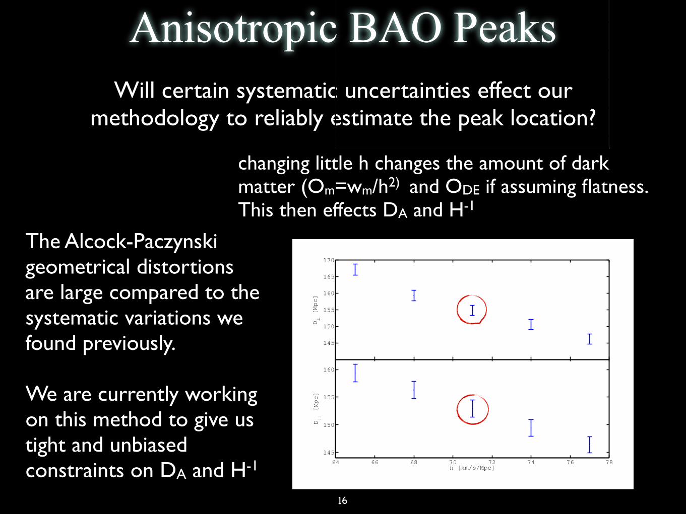
Will certain systematic uncertainties effect our methodology to reliably estimate the peak location?


163 164 165 166 167 168 169

156

157

158

159

160

161

162

163

D⊥ [Mpc]

D|| [Mpc]


64 66 68 70 72 74 76 78

145

150

155

160

D|| [Mpc]

h [km/s/Mpc]

145

150

155

160

165

170

D⊥ [Mpc]


4 TESTS ON SIMULATED DATA

In this section we test our methodology on simulated mockdata and check if we can recover the fiducial parameters.

4.1 Data

In order to check the validity of our overall approach, wetest it against simulations. We use the PTHALO mock galaxycatalogs created by Manera et al. (2012), which are de-signed to investigate the various systematics in the galaxysample from Data Release 11 (DR11) of the Baryon Oscil-lation Spectroscopic Survey (BOSS) (Schlegel et al. 2009;Eisenstein et al. 2011; Anderson et al. 2012), referred toas the “CMASS” galaxy sample. In constructing the mockgalaxy catalogs, (Manera et al. 2012) utilized second-orderLagrangian perturbation theory (2LPT) for the galaxy clus-tering driven by gravity, which enables the creation of amock catalog much faster than running an N -body simula-tion. The mocks catalogs constitute 600 density field realiza-tions which span the redshift range of the observed galaxiesin our sample i.e. 0.43 < z < 0.7. Each catalog contains

7 105 galaxies, 90% of which are central galaxies resid-ing in dark matter halos of 1013h1M.

4.2 results

5 CONCLUSIONS

We have investigated the sensitivity of the shape of the BAOring to various systematics. We find that the shape of theBAO ring is invariant to non-linearities in the density field,non-linear FoG distortions and unknown shape change inthe primordial spectra quantified using h. This invarianceallowed us to focus on measurements of the AP e↵ect andto infer cosmological parameters pertaining to the expansionhistory.

We tested this methodology using mock galaxy cata-logues and found that we can recover the input cosmology....

ACKNOWLEDGEMENTS

Thanks to all the people.....

REFERENCES

Alcock, C., & Paczynski, B. 1979, Nature, 281, 358Anderson, L., Aubourg, E., Bailey, S., et al. 2012, MNRAS,427, 3435

Ballinger, W.E., Peacock, J.A., & Heavens, A.F. 1996, MN-RAS, 282, 877

Beutler, F., Saito, S., Seo, H.-J., et al. 2013, MNRAS, 443,1065

Blake, C., Glazebrook, K., Davis, T. M., 2011, MNRAS,418, 1725

Chuang, C.-H., & Wang, Y. 2012, MNRAS, 426, 226Eisenstein, D. J., Weinberg, D. H., Agol, E., et al. 2011,APJ, 142, 72

Jeong, D., Dai, L., Kamionkowski, M., & Szalay, A.S. 2014,arXiv:1408.4648

Lavaux, G., & Wandelt, B.D. 2012, ApJ, 754, 109Linder, E.V., Minji, O., Okumura, T., Sabiu, C.G., & Song,Y.-S. 2014, Phys. Rev. D., 89, 063525

M. Manera, R. Scoccimarro, W. J. Percival, L. Samushia,C. K. McBride, A. Ross, R. Sheth and M. White et al.,Mon. Not. Roy. Astron. Soc. 428, no. 2, 1036 (2012)

Marinoni, C., & Buzzi, A. 2010, Nature, 468, 539Matsubara T., & Suto, Y. 1996, ApJ, 470, L1Outram, P.J., Shanks, T., Boyle, B.J., Croom, S.M., Hoyle,F., Loaring, N.S., Miller, L., & Smith, R.J. 2004, MNRAS,348, 745

Perlmutter, S., Aldering, G., Goldhaber, G., et al. 1999,ApJ, 517, 565

Reid, B. A., Samushia, L., White, M., et al. 2012, MNRAS,426, 2719

Riess, A. G., Filippenko, A. V., Challis, P., et al. 1998, AJ,116, 1009

Ryden, B.S. 1995, ApJ, 452, 25Schlegel, D., White, M., & Eisenstein, D. 2009, astro2010:The Astronomy and Astrophysics Decadal Survey, 2010,314

Song, Y.-S., et al. 2014, arXiv:1407.2257

c 0000 RAS, MNRAS 000, 000–000

Lord of the (BAO) Ring 3

D// [Mpc/h]

D⊥ [Mpc/h]

102 103 104 105 106102

102.5

103

103.5

104

104.5

105

105.5

106


D⊥ [Mpc/h]

D|| [Mpc/h]

102 103 104 105 106 107 108 109 110 111

102

103

104

105

106

107

108

xi−sigma−pi−fid

xi−sigma−pi−hp−3


3.1 Velocities

We first consider the fingers-of-god e↵ect where the galaxydistribution is elongated in redshift space, with an axis ofelongation pointed toward the observer. It is caused by aDoppler shift associated with the random peculiar velocitiesof galaxies bound in structures such as clusters. The devi-ation from the Hubble’s law relationship between distanceand redshift is altered, and this leads to inaccurate distancemeasurements.

We now proceed to check if the FoG distortion e↵ectsthe BAO peak position. In Fig.5 we show the derived dis-tance measurements using models with various v choices,of 0, 2, 4, 6, 8 Mpc/h. We find no significant trend or devi-ation with these values of v with either D// or D? and allmeasurements lie within a 1% error margin.

3.2 Non-linear

Comparing linear theory prediction with RegPT ref ref

151 152 153 154 155 156 157 158

148

149

150

151

152

153

154

155

D⊥ [Mpc]

D|| [Mpc]


D⊥ [Mpc]

D|| [Mpc]

153.5 154 154.5 155 155.5 156

151

151.5

152

152.5

153

153.5

154

154.5

155


3.3 Hubble value

In Fig.6 we show the e↵ect of changing the hubble constantin the primordial spectra on the derived distance measures.However we do not include the AP distortion in this theo-retical template. We find that variations of ±6Mpc in h donot alter the obtained values of D// and D?.

3.4 Bias

In Fig.7 we show the e↵ect of changing the bias factor ofthe theoretical 2pcf on the derived distance measures. Sincethe bias a linear we should not expect a shift in the BAOpeak position however we investigate this change in the casethat our minimal model can still fit the peak position with-out introducing any systematic variation due to inaccuratefitting. We find that values of b = 1.2, 1.4,1.6, 1.8 all giveconsistent values of D// and D?.

3.5 Alcock-Paczynski

The AP e↵ect is now included ....In Fig.8 we

c 0000 RAS, MNRAS 000, 000–000

We show the derived distance measurements using models with various σv choices, of 0, 2, 4, 6, 8 Mpc/h. No significant trend or deviation with these values of σv with either D// or D⊥ and all measurements lie within a 1% error margin.

we show the effect of changing the bias factor on the derived distance measures. We find that values of b = 1.2, 1.4,1.6, 1.8 all give consistent values of D// and D⊥.


We also checked the effect of shifting the overall shape of the spectrum and looked at Linear vs NonLinear templates. However all give 1% level or less deviations on the distances. So our fitting function seems to have enough freedom to accommodate many unknown factors that, in the end, we don’t want to deal with!

16

Will certain systematic uncertainties effect our methodology to reliably estimate the peak location?

changing little h changes the amount of dark matter (Om=wm/h2) and ODE if assuming flatness. This then effects DA and H-1


163 164 165 166 167 168 169

156

157

158

159

160

161

162

163

D⊥ [Mpc]

D|| [Mpc]


64 66 68 70 72 74 76 78

145

150

155

160

D|| [Mpc]

h [km/s/Mpc]

145

150

155

160

165

170

D⊥ [Mpc]


4 TESTS ON SIMULATED DATA

In this section we test our methodology on simulated mockdata and check if we can recover the fiducial parameters.

4.1 Data

In order to check the validity of our overall approach, wetest it against simulations. We use the PTHALO mock galaxycatalogs created by Manera et al. (2012), which are de-signed to investigate the various systematics in the galaxysample from Data Release 11 (DR11) of the Baryon Oscil-lation Spectroscopic Survey (BOSS) (Schlegel et al. 2009;Eisenstein et al. 2011; Anderson et al. 2012), referred toas the “CMASS” galaxy sample. In constructing the mockgalaxy catalogs, (Manera et al. 2012) utilized second-orderLagrangian perturbation theory (2LPT) for the galaxy clus-tering driven by gravity, which enables the creation of amock catalog much faster than running an N -body simula-tion. The mocks catalogs constitute 600 density field realiza-tions which span the redshift range of the observed galaxiesin our sample i.e. 0.43 < z < 0.7. Each catalog contains

7 105 galaxies, 90% of which are central galaxies resid-ing in dark matter halos of 1013h1M.

4.2 results

5 CONCLUSIONS

We have investigated the sensitivity of the shape of the BAOring to various systematics. We find that the shape of theBAO ring is invariant to non-linearities in the density field,non-linear FoG distortions and unknown shape change inthe primordial spectra quantified using h. This invarianceallowed us to focus on measurements of the AP e↵ect andto infer cosmological parameters pertaining to the expansionhistory.

We tested this methodology using mock galaxy cata-logues and found that we can recover the input cosmology....

ACKNOWLEDGEMENTS

Thanks to all the people.....

REFERENCES

Alcock, C., & Paczynski, B. 1979, Nature, 281, 358Anderson, L., Aubourg, E., Bailey, S., et al. 2012, MNRAS,427, 3435




Chuang, C.-H., & Wang, Y. 2012, MNRAS, 426, 226Eisenstein, D. J., Weinberg, D. H., Agol, E., et al. 2011,APJ, 142, 72


Lavaux, G., & Wandelt, B.D. 2012, ApJ, 754, 109Linder, E.V., Minji, O., Okumura, T., Sabiu, C.G., & Song,Y.-S. 2014, Phys. Rev. D., 89, 063525

M. Manera, R. Scoccimarro, W. J. Percival, L. Samushia,C. K. McBride, A. Ross, R. Sheth and M. White et al.,Mon. Not. Roy. Astron. Soc. 428, no. 2, 1036 (2012)

Marinoni, C., & Buzzi, A. 2010, Nature, 468, 539Matsubara T., & Suto, Y. 1996, ApJ, 470, L1Outram, P.J., Shanks, T., Boyle, B.J., Croom, S.M., Hoyle,F., Loaring, N.S., Miller, L., & Smith, R.J. 2004, MNRAS,348, 745

Perlmutter, S., Aldering, G., Goldhaber, G., et al. 1999,ApJ, 517, 565

Reid, B. A., Samushia, L., White, M., et al. 2012, MNRAS,426, 2719

Riess, A. G., Filippenko, A. V., Challis, P., et al. 1998, AJ,116, 1009

Ryden, B.S. 1995, ApJ, 452, 25Schlegel, D., White, M., & Eisenstein, D. 2009, astro2010:The Astronomy and Astrophysics Decadal Survey, 2010,314

Song, Y.-S., et al. 2014, arXiv:1407.2257

c 0000 RAS, MNRAS 000, 000–000

The Alcock-Paczynski geometrical distortions are large compared to the systematic variations we found previously.

We are currently working on this method to give us tight and unbiased constraints on DA and H-1


17

Clustering ShellsEven without a standard ruler, we can measure the clustering along and perpendicular to the line of sight and thus constrain the combination of DA and H-1

In this statistical analysis we aim to constrain the AP effect.Rather than using the BAO peak position, we use the integrated clustering signal in different directions.

Pictorially what happens to cosmological positions if translated using an incorrect cosmological model.

4 Xiao-Dong Li, Changbom Park, Cristiano G. Sabiu and Juhan Kim

To probe the anisotropy, ξ is measured at different di-rections, and integrated over the interval ∆s = smax − smin.We evaluate,

ξ∆s(µ) ≡

∫ smax

smin

ξ(s, µ) ds. (5)

We limit the integral at both small and large scales. At smallscales the shape of ξ∆s(µ) is seriously distorted by the FoGeffect, and the distortion is more significant at lower redshiftwhere structure undergoes more non-linear growth. This in-troduces redshift evolution in ξ∆s(µ) which is rather diffi-cult to model. At large scales the measurement is dominatedby noise due to poor statistics. In our analysis, we choosesmin = 6 Mpc/h and smax = 50 Mpc/h, which we found toprovide consistent and unbiased results.

As an example Figure 2 shows how the 2pCF is affectedby AP and volume effects in the Ωm = 0.41, w = −1.3cosmology. In choosing incorrect cosmological parameters,we expect the 2pCF to be influenced in three ways. First,as a result of the AP effect, structures appear compressedin the radial direction. This induces a nonuniform variationin ξ∆s(µ) as a function of angle. Second, as a result of thevolume effect, the size of structures are shrunk. For example,a structures whose original size is s0 = 50 Mpc/h will showsup with a size s1 < 50 Mpc/h. As a result, the amplitudeof ξ∆s(µ) changes. Finally, as another consequence of thevolume effect, in the wrong cosmology structures on largerscales enter the statistics. For example, halos within the bluesolid box are not considered in the correct cosmology, butthey are taken into consideration in the wrong cosmology, asshown by the black dashed box. This also results in a changein the amplitude of ξ∆s(µ) since the binning in s, µ-spacewill be inconsistent between different cosmological models.The combined effects of choosing an incorrect cosmology onshear and volume have been noted by Park & Kim (2010),who used the volume effects measured by the genus statisticto constrain the expansion history of the universe.

5 RESULT

Figure 3 shows the ξ∆s measured from HR3 mock surveys,adopting the correct cosmology (left), the Ωm = 0.11, w =−0.7 cosmology (middle), and the Ωm = 0.41, w = −1.3cosmology (right). To study the redshift evolution, we dividethe redshift range z = 0− 1.5 into five equal-width redshiftbins 1. To measure anisotropy, we further divide the fullangular range µ = 0 − 1 is into 10 equal-width bins. So wehave

ξ∆s(zi, µj) ≡ ξ∆s in the i − th redshift bin, j − th µ bin(6)

where i = 1, 2, ..., 5, j = 1, 2, ...10. Measurements with-out/with considering RSD effect are plotted in solid/dashedlines, respectively.

The result for the correct cosmology is plotted in theupper left panel of Figure 3. In the absence of RSD, we ob-tain flat curves of ξ∆s(µ) in all redshift bins, with the am-plitude slightly different from one redshift bin to another.

1 We do not show the result of the first redshift bin, which isnoisy due to poor statistics.

This difference can arise from two sources; (a) The growthof clustering with the decreasing of redshift (b) The redshiftevolution of the bias of halos having the same comoving den-sity. The result is significantly changed when we include theRSD effect. Near the LOS direction (µ → 1), structures arecompressed due to the Kaiser effect, so the value of ξ∆s(µ)is smaller compared with measurements near the tangentialdirection2. But it should be noted that the shape of ξ∆s(µ)is nearly the same at all redshifts, indicating the small red-shift dependence of the RSD effect. It is this observation thatmakes our method both feasible and statistically powerful.Even though the 2pCF becomes very anisotropic in redshiftspace, the anisotropy due to RSD does not change much asa function of redshift and its redshift-dependence is dom-inated by the geometric effects introduced by the adoptedcosmology.

The results of the Ωm = 0.11, w = −0.7 and Ωm = 0.41,w = −1.3 cosmologies are plotted in the middle and rightpanels, respectively. We can see that ξ∆s is significantly al-tered by the volume and AP effects. In the Ωm = 0.41,w = −1.3 cosmology, the shrinkage of comoving volume sup-presses the amplitude of ξ∆s(µ), and the LOS shape com-pression of structures results in a suppression of amplitudein the LOS direction compared with the tangential. Botheffects become increasingly more significant at higher red-shift. Similarly, in the Ωm = 0.11, w = −0.7 cosmology, wesee an enhancement of amplitude and relative enhancementin the LOS direction, and these effects are more significantat earlier times.

In real observational data the redshift evolution of thebias of observed galaxies is difficult to model. Thus to miti-gate this systematic uncertainty we wish to rely on the shapeof ξ∆s(µ), rather than its amplitude. In the lower panel ofFigure 3, we show the normalized ξ∆s(µ) in each redshiftbin, defined as

ξ∆s(µ) ≡ξ∆s(µ)

∫ 1

0ξ∆s(µ) dµ

. (7)

In the correct cosmology ξ∆s at different redshifts are iden-tical to each other, while in the wrong cosmologies we seeclear redshift evolution.

Overall, the effect of RSD on the 2pCF is large but itsredshift dependence is small. Even with RSD, we can stillcorrectly determine the true cosmology by using the relativechange of ξ∆s with redshift. Based on this fact, we define ourχ2 as follows

χ2 ≡

4∑

i=1

10∑

j=1

[ξ∆s(zi, µj)− ξ∆s(z5, µj)]2

σ2ξ∆s(zi,µj)

+ σ2ξ∆s(z5,µj)

. (8)

The 2pCF measured in the 1-4 redshift bins are compared(or normalized) to the measurement in the last redshift bin.This χ2 will prefer minimal shape change over the redshiftrange, with little of no weight given to the amplitude of theclustering statistic.

Similar to Li et al. (2014), we further correct the resid-ual RSD effect, i.e., the following quantity is computed inthe correct cosmology and subtracted from our results,

2 The FoG effect will enhance ξ∆s(µ) in the LOS direction. Itdoes not significantly show up in our figures since we impose thecut smin = 6 Mpc/h.

c© 2002 RAS, MNRAS 000, 1–8

with Xiao-Dong Li & Changbom Park (KIAS)

Cosmological Constraints from the Redshift Dependence of AP and Volume Effects 3

Figure 1. The redshift dependence of AP and volume effect in two wrongly assumed cosmologies Ωm = 0.41, w = −1.3 and Ωm = 0.11,w = −0.7, assuming a true cosmology of Ωm = 0.26, w = −1. Upper panel shows the apparent distortion of four perfect squares. Theapparently distorted shapes are plotted in red solid lines. The underlying true shapes are plotted in blue dashed lines. Lower panel showsthe evolution of Equations (1) and (2). In our mock surveys we split the samples at z = 0.3, 0.6, 0.9 and 1.2, as marked by the verticallines.

separation. Then the Physically Self Bound (PSB) subha-los that are gravitationally self-bound and tidally stable areidentified (Kim & Park 2006).

An all-sky, very deep light cone survey reaching redshiftz = 4.3 was made by placing an observer located at the cen-ter of the box. The co-moving positions and velocities of allCDM particles are saved as they cross the past light coneand PSB subhalos are identified from this particle data. Tomatch the observations of recent LRG surveys (Choi et al.2010; Gott et al. 2009, 2008), a volume-limited sample of ha-los with constant number density of 3×10−4(h−1Mpc)−3 areselected by imposing a minimum halo mass limit and red-shift range. The light cone survey sample consists of subha-los at different redshifts, and thus their redshift dependenceon velocities and evolution of clustering are automaticallyincluded. The peculiar velocity of the sub halo is set to thatof the most-bound particle in that subhalo.

We divide the whole-sky survey sample into eight equalsky area subsamples and impose the redshift range z =0 − 1.5. This mock data will be relevant for future galaxyspectroscopic surveys (e.g. DESI Levi et al. 2013).

4 METHODOLOGY

We probe the effects discussed in §2 using the 2pCF. The2pCF is a mature statistic in cosmology and its optimalestimation considers minimal variance while dealing withcomplicated masks and selection functions. The most com-monly adopted formulation is that of the Landy-Szalay es-timator (Landy & Szalay 1993),

ξ(s, µ) =DD − 2DR +RR

RR, (4)

where DD is the number of galaxy–galaxy pairs, DR thenumber of galaxy-random pairs, and RR is the number ofrandom–random pairs, all separated by a distance definedby s ± ∆s and µ ± ∆µ, where s is the distance betweenthe pair and µ = cos(θ), with θ being the angle betweenthe line joining the pair of points and the LOS direction.This statistic therefore captures the radial anisotropy of theclustering signal.

The random point catalogue constitutes an unclusteredbut observationally representative sample of our mock sur-veys. To reduce the statistical variance of the estimator weuse ∼15 times as many randoms as we have galaxies.

c© 2002 RAS, MNRAS 000, 1–8

For Om=0.41, w=-1.3, we see a stretch of the shape in the LOS direction and magnification of the volume

For Om=0.11, w=-0.7, we see a LOS shape compression and volume shrinkage.

18

Clustering ShellsThe integrated clustering strength as a function of angle at varies redshifts.

In the no RSD case in the correct cosmology the curves are flat. In the wrong cosmologies they are distorted.

With RSDs we see much more variation in shape and amplitude.

If we normalise the curves, then we remove amplitude information and minimise the volume effect thus focusing on a pure AP measurement.


Figure 3. The 2pCF measured in four redshift bins, in the correct cosmology (left) and two wrongly assumed cosmologies (middle:Ωm = 0.11, w = −0.7; right: Ωm = 0.41, w = −1.3). The clustering signal is measure as a function of 1 − µ ,where µ = cos(θ) and θis the angle between the LOS and the vector joining the pair of galaxies. Dashed and solid lines show the results with and without theRSD effect, respectively. Upper panel: In the wrongly assumed cosmologies, we observe a clear change in the amplitudes and shapes ofξ due to the volume and AP effect. Additionally, due to the redshift dependence of volume and AP effect, the amplitudes and shapes inthe four redshift bins are different from each other. Lower panel: The same as the upper panel, except that the amplitudes of curves arenormalized to 1.

constraints become much tighter, with δΩm ∼ 0.007 andδw ∼ 0.035. Also, the direction of degeneracy changes andis very different from mainstream techniques of CMB, SNIaand BAO, meaning that combining our method with thesetechniques can significantly improve the constraint. To im-plement it in real observational cases, it is necessary tomodel the evolution of the clustering amplitude for the ob-served galaxies.

6 CONCLUSION

We have presented a new anisotropic clustering statistic thatcan probe the cosmic expansion history, while making mini-mal assumptions about the underlying cosmological model.We measure the integrated 2pCF, ξ∆s(µ) ≡

∫ smax

sminξ(s, µ)ds,

as a function of direction µ. The amplitude of ξ∆s(µ) is af-fected by the volume effect, and the shape is affected bythe AP effect. Due to the redshift dependence of the volumeand AP effects, in wrongly adopted cosmologies there areredshift evolutions of the amplitude and shape. The RSD

c© 2002 RAS, MNRAS 000, 1–8

Using mock many catalogues drawn from the Horizon Run simulations (from Juhan Kim, KIAS)

19

Clustering Shells

The clustering shells provide a similar constraints to those obtained from standard BAO analysis.

The volume effect, which causes redshift evolution in the amplitude of 2pCF, leads to very tight constraint on cosmological parameters. But it suffers from systematic effects of growth of clustering and the variation of galaxy sample with redshift.

Cosmological Constraints from the Redshift Dependence of AP and Volume Effects 7

Figure 4. Left: Expected cosmological constraints from a 1/8-sky, z < 1.5 survey with a constant galaxy number density of n = 3×10−4 .We achieve unbiased constraints with δw ∼ 0.1 and δΩm ∼ 0.03 by comparing the shapes of ξ∆s(µ) measured in different redshift bins.The gray contours denote 1, 2, 3σ. Right: Here we use the unnormalized ξ∆s(µ), which is sensitive to the volume change and thus providesmuch tighter constraints. Although to use this in practice would mean overcoming some observational systematic uncertainties like galaxyevolution and selection bias.

effect due to galaxy peculiar velocities, although having astrong effect on ξ∆s(µ), does not exhibit significant redshiftevolution. Thus by focusing on the redshift dependence ofξ∆s(µ), we are able to derive accurate and unbiased esti-mates of cosmological parameters in spite of contaminationinduced by RSD.

The concept of this paper is similar to Li et al. (2014),where the redshift dependence of the AP effect is mea-sured from the anisotropy in the galaxy density gradientfield. However, in this paper we choose a different statisticalmethod, i.e. the 2pCF. They differ from each other in severalaspects. 1) Using the 2pCF method it is more convenient tochoose the scales we investigate. 2) The advantage of thedensity gradient field method is that, it allows us to utilizethe information on small scales of ∼10 Mpc/h (dependingon the scale of smoothing). 3) In the 2pCF method we areable to probe the volume effect, which is not possible for thegalaxy density field method. 4) The 2pCF is a mature statis-tic in cosmology and its optimal estimation and statisticalproperties are well understood.

The volume effect, which causes redshift evolution in theamplitude of 2pCF, leads to very tight constraint on cosmo-logical parameters. But it suffers from systematic effects ofgrowth of clustering and the variation of galaxy sample withredshift. It would be great if one can reliably model thesetwo effects and utilize the volume effect. In case that thesystematic effect can not be correctly modelled, one can fo-cus on the AP effect by normalizing the amplitude of ξ∆s(µ)and just investigating the redshift evolution of the shape.

When dealing with real observational data, it will be im-portant to accurately model the galaxy clustering to removethe residual RSD effects on the 2pCF. It will also requirethe handling of various observation effects such as surveygeometry, fiber collisions, etc. We will report the results ofsuch investigations in forthcoming studies.

ACKNOWLEDGMENTS

We thank the Korea Institute for Advanced Study for pro-viding computing resources (KIAS Center for AdvancedComputation Linux Cluster System). We thank SeokcheonLee and Graziano Rossi for many helpful discussions.

REFERENCES

Alcock, C., & Paczynski, B. 1979, Nature, 281, 358Anderson, L., Aubourg, E., Bailey, S. et al. 2014, MNRAS,441, 24




Choi, Y.-Y., Park, C., Kim, J., Gott, J.R., Weinberg, D.H.,Vogeley, M.S., & Kim, S.S. 2010, ApJS, 190, 181

Chuang, C.-H., & Wang, Y. 2012, MNRAS, 426, 226Gott, J.R., Choi, Y.-Y., Park, C., & Kim, J. 2009, ApJ,695, L45

Gott, J.R., Hambrick, D.C., Vogeley, M.S., Kim, J., Park,C., Choi, Y.-Y., Cen, R., Ostriker, J.P., & Nagamine, K.2008, ApJ, 675, 16


Kim, J., & Park, C. 2006, ApJ, 639, 600Kim, J., Park, C., Gott, J. R., III, & Dubinski, J. 2009,ApJ, 701, 1547

Kim, J., Park, C., Rossi, G., Lee, S.M., & Gott, J.R., 2011,JKAS, 44, 217

Komatsu, E., Smith, K. M., Dunkley, J., et al. 2011, ApJS,192, 18

S. D. Landy, & A. S. Szalay, 1993, ApJ, 412, 64

c© 2002 RAS, MNRAS 000, 1–8


which leads to apparent anisotropy even if the adopted cos-mology is correct (Ballinger Peacock & Heavens 1996). In Liet al. (2014) we proposed a new method utilizing the red-shift dependence of AP effect to overcome the RSD problem,which uses the isotropy of the galaxy density gradient field.We found that the redshift dependence of the anisotropycreated by RSD is much less significant compared with theanisotropy caused by AP. Thus we measured the redshift de-pendence of the galaxy density gradient field, which is lessaffected by RSD, but still sensitive to cosmological parame-ters.

The two-point correlation analysis is the most widelyused method to study the large scale clusterings of galax-ies. So, in this paper we revisit the topic of Li et al. (2014)using the galaxy two-point correlation function (2pCF). Byinvestigating the redshift dependence of anisotropic galaxyclustering we can measure the AP effect despite of contam-ination from RSD. Moreover, if the redshift evolution ofgalaxy bias can be reliably modelled, then we can measurethe redshift evolution of volume effect from the amplitudeof 2pCF. The change of the comoving volume size is anotherconsequence of a wrongly adopted cosmology, which has mo-tivated methods constraining cosmological parameters fromnumber counting of galaxy clusters (Press & Shechter 1974;Viana & Liddle 1996) and topology (Park & Kim 2010).

The outline of this paper proceeds as follows. In §2 webriefly review the nature and consequences of the AP effectand volume changes when performing coordinate transformsin a cosmological context. In §3 we describe the N-bodysimulations and mock galaxy catalogues that are used totest our methodology. In §4 we will describe our new analysismethod for quantifying the anisotropic clustering as well asproposing a way to deal with the RSD that are convolvedwith the AP distortion. Here we will also present results ofour optimised estimator. We conclude in §5.

2 THE AP AND VOLUME EFFECT DUE TO

WRONGLY ASSUMED COSMOLOGICAL

PARAMETERS

The AP and volume effect due to wrongly assumed cosmo-logical parameters are shown in the upper panel of Figure1. Suppose that the true cosmology is a flat ΛCDM withpresent density parameter Ωm = 0.26 and standard darkenergy equation of state (EoS) w = −1. If we were to dis-tribute four perfect squares at various distances from 500Mpc/h to 3,000 Mpc/h, and an observer were to measuretheir redshifts and compute their positions and shapes us-ing redshift-distance relations of two incorrect cosmologies:

(i) Ωm = 0.41, w = −1.3,(ii) Ωm = 0.11, w = −0.7,

the shapes of the squares appear distorted (AP effect), andtheir volumes are changed (volume effect). In the cosmolog-ical model (ii) with Ωm = 0.11, w = −0.7, we see a stretchof the shape in the LOS direction (hereafter “LOS shapestretch”) and magnification of the volume (hereafter “vol-ume magnification”), while in the model with Ωm = 0.41,w = −1.3, we see opposite effects, with LOS shape compres-sion and volume shrinkage.

The degree of LOS shape stretch and volume magnifi-cation can be described by the following quantities

[∆r‖/∆r⊥]wrong

[∆r‖/∆r⊥]true=

[DA(z)H(z)]true[DA(z)H(z)]wrong

, (1)

Volumewrong

Volumetrue=

[DA(z)2/H(z)]wrong

[DA(z)2/H(z)]true, (2)

where ∆r‖, ∆r⊥ are the angular and radial sizes of the ob-jects, and “true” and “wrong” denote the values of quanti-ties in the true cosmology and wrongly assumed cosmology.DA and H are the angular diameter distance and Hubbleparameter, respectively. In the particular case of a flat uni-verse with constant dark energy EoS, they take the formsof

H(z) = H0

√

Ωma−3 + (1− Ωm)a−3(1+w),

DA(z) =1

1 + zr(z) =

11 + z

∫ z

0

dz′

H(z′), (3)

where a = 1/(1 + z) is the cosmic scale factor, H0 is thepresent value of Hubble parameter and r(z) is the comovingdistance.

In the lower panel of Figure 1, we plot the degree ofLOS shape stretch and volume magnification as functionsof redshift. In cosmology (i), both quantities have valueless than 1, indicating LOS shape compression and volumeshrink. The effect in cosmology (ii) is slightly more subtle.At low redshift, the effect of dark energy is important, andthere is LOS shape compression and volume reduction dueto the quintessence like dark energy EoS. However, at higherredshift the role of dark matter is more important, and wesee LOS shape stretch and volume magnification due to thesmall Ωm.

More importantly, Figure 1 highlights the redshift de-pendence of the AP and volume effects. For example, in thecosmology with Ωm = 0.41, w = −1.3, both the LOS shapestretch and volume magnification become more significantwith increasing redshift. In the cosmology with Ωm = 0.11,w = −0.7, not only do the magnitudes of the effects evolvewith redshift, but there is also a turnover from LOS shapecompression and volume shrink at lower redshift to LOSshape stretch and volume magnification at higher redshift.

3 DATA

We test the methodology using mock surveys constructedfrom one of the Horizon Run simulations, HR3. HR3 are asuite of large volume N-body simulations that have resolu-tions and volumes capable of reproducing the observationalstatistics of many current major redshift surveys like SDSSBOSS etc (Park et al. 2005; Kim et al. 2009, 2011). HR3adopts a flat-space ΛCDM cosmology with the WMAP 5year parameters Ωm = 0.26, H0 = 72km/s/Mpc, ns = 0.96and σ8 = 0.79 (Komatsu et al. 2011). The simulation wasmade in a cube of volume (10.815 h−1Gpc)3 using 71203

particles with particle mass of 1.25 × 1011h−1M% .The simulations were integrated from z = 27 and

reached z = 0 after making Nstep = 600 timesteps. Darkmatter halos were identified using the Friend-of-Friend algo-rithm with the linking length of 0.2 times the mean particle

c© 2002 RAS, MNRAS 000, 1–8


which leads to apparent anisotropy even if the adopted cos-mology is correct (Ballinger Peacock & Heavens 1996). In Liet al. (2014) we proposed a new method utilizing the red-shift dependence of AP effect to overcome the RSD problem,which uses the isotropy of the galaxy density gradient field.We found that the redshift dependence of the anisotropycreated by RSD is much less significant compared with theanisotropy caused by AP. Thus we measured the redshift de-pendence of the galaxy density gradient field, which is lessaffected by RSD, but still sensitive to cosmological parame-ters.

The two-point correlation analysis is the most widelyused method to study the large scale clusterings of galax-ies. So, in this paper we revisit the topic of Li et al. (2014)using the galaxy two-point correlation function (2pCF). Byinvestigating the redshift dependence of anisotropic galaxyclustering we can measure the AP effect despite of contam-ination from RSD. Moreover, if the redshift evolution ofgalaxy bias can be reliably modelled, then we can measurethe redshift evolution of volume effect from the amplitudeof 2pCF. The change of the comoving volume size is anotherconsequence of a wrongly adopted cosmology, which has mo-tivated methods constraining cosmological parameters fromnumber counting of galaxy clusters (Press & Shechter 1974;Viana & Liddle 1996) and topology (Park & Kim 2010).

The outline of this paper proceeds as follows. In §2 webriefly review the nature and consequences of the AP effectand volume changes when performing coordinate transformsin a cosmological context. In §3 we describe the N-bodysimulations and mock galaxy catalogues that are used totest our methodology. In §4 we will describe our new analysismethod for quantifying the anisotropic clustering as well asproposing a way to deal with the RSD that are convolvedwith the AP distortion. Here we will also present results ofour optimised estimator. We conclude in §5.

2 THE AP AND VOLUME EFFECT DUE TO

WRONGLY ASSUMED COSMOLOGICAL

PARAMETERS

The AP and volume effect due to wrongly assumed cosmo-logical parameters are shown in the upper panel of Figure1. Suppose that the true cosmology is a flat ΛCDM withpresent density parameter Ωm = 0.26 and standard darkenergy equation of state (EoS) w = −1. If we were to dis-tribute four perfect squares at various distances from 500Mpc/h to 3,000 Mpc/h, and an observer were to measuretheir redshifts and compute their positions and shapes us-ing redshift-distance relations of two incorrect cosmologies:

(i) Ωm = 0.41, w = −1.3,(ii) Ωm = 0.11, w = −0.7,

the shapes of the squares appear distorted (AP effect), andtheir volumes are changed (volume effect). In the cosmolog-ical model (ii) with Ωm = 0.11, w = −0.7, we see a stretchof the shape in the LOS direction (hereafter “LOS shapestretch”) and magnification of the volume (hereafter “vol-ume magnification”), while in the model with Ωm = 0.41,w = −1.3, we see opposite effects, with LOS shape compres-sion and volume shrinkage.

The degree of LOS shape stretch and volume magnifi-cation can be described by the following quantities

[∆r‖/∆r⊥]wrong

[∆r‖/∆r⊥]true=

[DA(z)H(z)]true[DA(z)H(z)]wrong

, (1)

Volumewrong

Volumetrue=

[DA(z)2/H(z)]wrong

[DA(z)2/H(z)]true, (2)

where ∆r‖, ∆r⊥ are the angular and radial sizes of the ob-jects, and “true” and “wrong” denote the values of quanti-ties in the true cosmology and wrongly assumed cosmology.DA and H are the angular diameter distance and Hubbleparameter, respectively. In the particular case of a flat uni-verse with constant dark energy EoS, they take the formsof

H(z) = H0

√

Ωma−3 + (1− Ωm)a−3(1+w),

DA(z) =1

1 + zr(z) =

11 + z

∫ z

0

dz′

H(z′), (3)

where a = 1/(1 + z) is the cosmic scale factor, H0 is thepresent value of Hubble parameter and r(z) is the comovingdistance.

In the lower panel of Figure 1, we plot the degree ofLOS shape stretch and volume magnification as functionsof redshift. In cosmology (i), both quantities have valueless than 1, indicating LOS shape compression and volumeshrink. The effect in cosmology (ii) is slightly more subtle.At low redshift, the effect of dark energy is important, andthere is LOS shape compression and volume reduction dueto the quintessence like dark energy EoS. However, at higherredshift the role of dark matter is more important, and wesee LOS shape stretch and volume magnification due to thesmall Ωm.

More importantly, Figure 1 highlights the redshift de-pendence of the AP and volume effects. For example, in thecosmology with Ωm = 0.41, w = −1.3, both the LOS shapestretch and volume magnification become more significantwith increasing redshift. In the cosmology with Ωm = 0.11,w = −0.7, not only do the magnitudes of the effects evolvewith redshift, but there is also a turnover from LOS shapecompression and volume shrink at lower redshift to LOSshape stretch and volume magnification at higher redshift.

3 DATA

We test the methodology using mock surveys constructedfrom one of the Horizon Run simulations, HR3. HR3 are asuite of large volume N-body simulations that have resolu-tions and volumes capable of reproducing the observationalstatistics of many current major redshift surveys like SDSSBOSS etc (Park et al. 2005; Kim et al. 2009, 2011). HR3adopts a flat-space ΛCDM cosmology with the WMAP 5year parameters Ωm = 0.26, H0 = 72km/s/Mpc, ns = 0.96and σ8 = 0.79 (Komatsu et al. 2011). The simulation wasmade in a cube of volume (10.815 h−1Gpc)3 using 71203

particles with particle mass of 1.25 × 1011h−1M% .The simulations were integrated from z = 27 and

reached z = 0 after making Nstep = 600 timesteps. Darkmatter halos were identified using the Friend-of-Friend algo-rithm with the linking length of 0.2 times the mean particle

c© 2002 RAS, MNRAS 000, 1–8

We construct a likelihood function by requiring that the shape change as a function of redshift is minimized. Of course there is a redshift evolution of the clustering, however this is modeled to first-order using N-body simulations.

Conclusions

Davis etal 2011

- we have shown that the anisotropic BAO peak positions are unaffected by the systematics we consider, namely bias, FoG, non-linear templates.

- this method therefore provides an unbiased constraints on DA(z) and H-1(z).

- we are working now on the constraining power of this method considering current and future data from SDSS BOSS -> DESI.

- The anisotropic ‘clustering shells’ provide unbiased and tight constraints on w and Om, considering flat LCDM model.

- However more generally this methodology can be used to track the expansion history.

Cosmology Group at Korea Astronomy and Space Science Institute

Documents

Towards unbiased constraints on the expansion history from