Embed Size (px)
Citation preview

The copyright of this thesis rests with the University of Cape Town. No
quotation from it or information derived from it is to be published
without full acknowledgement of the source. The thesis is to be used
for private study or non-commercial research purposes only.
Univers
ity of
Cap
e Tow
n
Pattern recognition to detect fetal alcohol
syndrome using stereo facial images
Prepared by: Mahalingam Veeraragoo
Supervised by: T. S. Douglas
Department of Human Biology
University of Cape Town
10 May 2010
Univers
ity O
f Cap
e Tow
n

Declaration
I declare that this dissertation is my own, unaided work. It is being submitted in partial
fulfilment of the requirements for the degree of Msc(Med) in Biomedical Engineering at
the University of Cape Town. It has not been submitted before for any degree or exami-
nation in any other university.
Signature of Author . . . . . . . . . . . . . . . . . . . . . . . . . . . . . . . . . . . . . . . . . . . . . . . . . . . . . . . . . . . . . .
Cape Town
10 May 2010
i
Univers
ity O
f Cap
e Tow
n

Acknowledgements
I would like to thank Associate Professor T.S. Douglas for the precious opportunity pre-
sented to me and for all the help and guidance offered during the course of this degree.
I would also like to acknowledge Dr. Rolf P. Würtz and Manuel Günther from the Institut
für Neuroinformatik, Ruhr-Universität Bochum, Germany, who assisted me in the use of
the elastic bunch graph matching software.
Special thanks goes to Dr. T.E.M. Mutsvangwa for his continuous assistance with stereo-
photogrammetry, facial shape analysis, his permission to use his pictures in the thesis and
the fun trips to Ceres for data collection.
Thanks also goes to the Foundation for Alcohol Related Research (FARR) for making
data collection possible.
Finally I would like to thank my family for their lifelong support and encouragement.
ii
Univers
ity O
f Cap
e Tow
n

Abstract
Fetal alcohol syndrome (FAS) is a condition which is caused by excessive consumption
of alcohol by the mother during pregnancy. A FAS diagnosis depends on the presence of
growth retardation, central nervous system and neurodevelopment abnormalities together
with facial malformations. The main facial features which best distinguish children with
and without FAS are smooth philtrum, thin upper lip and short palpebral fissures. Diagno-
sis of the facial phenotype associated with FAS can be done using methods such as direct
facial anthropometry and photogrammetry.
The project described here used information obtained from stereo facial images and ap-
plied facial shape analysis and pattern recognition to distinguish between children with
FAS and control children. Other researches have reported on identifying FAS through the
classification of 2D landmark coordinates and 3D landmark information in the form of
Procrustes residuals. This project built on this previous work with the use of 3D informa-
tion combined with texture as features for facial classification.
Stereo facial images of children were used to obtain the 3D coordinates of those facial
landmarks which play a role in defining the FAS facial phenotype. Two datasets were
used: the first consisted of facial images of 34 children whose facial shapes had previously
been analysed with respect to FAS. The second dataset consisted of a new set of images
from 40 subjects.
Elastic bunch graph matching was used on the frontal facial images of the study popula-
iii
Univers
ity O
f Cap
e Tow
n
tion to obtain texture information, in the form of jets, around selected landmarks. Their
2D coordinates were also extracted during the process. Faces were classified using k-
nearest neighbor (kNN), linear discriminant analysis (LDA) and support vector machine
(SVM) classifiers. Principal component analysis was used for dimensionality reduction
while classification accuracy was assessed using leave-one-out cross-validation.
For dataset 1, using 2D coordinates together with texture information as features during
classification produced a best classification accuracy of 72.7% with kNN, 75.8% with
LDA and 78.8% with SVM. When the 2D coordinates were replaced by Procrustes resid-
uals (which encode 3D facial shape information), the best classification accuracies were
69.7% with kNN, 81.8% with LDA and 78.6% with SVM. LDA produced the most con-
sistent classification results.
The classification accuracies for dataset 2 were lower than for dataset 1. The different
conditions during data collection and the possible differences in the ethnic composition
of the datasets were identified as likely causes for this decrease in classification accuracy.
iv
Univers
ity O
f Cap
e Tow
n

Contents
Declaration i
Acknowledgements ii
Abstract iii
1 Introduction 2
1.1 Background . . . . . . . . . . . . . . . . . . . . . . . . . . . . . . . . . 2
1.2 Objectives and significance . . . . . . . . . . . . . . . . . . . . . . . . . 3
1.3 Thesis outline . . . . . . . . . . . . . . . . . . . . . . . . . . . . . . . . 4
2 Literature review 5
2.1 Fetal alcohol syndrome . . . . . . . . . . . . . . . . . . . . . . . . . . . 5
2.2 Direct anthropometry . . . . . . . . . . . . . . . . . . . . . . . . . . . . 6
2.2.1 Direct anthropometry for FAS diagnosis . . . . . . . . . . . . . . 6
2.3 Indirect anthropometry . . . . . . . . . . . . . . . . . . . . . . . . . . . 7
2.3.1 Photography . . . . . . . . . . . . . . . . . . . . . . . . . . . . 7
2.3.2 Stereo-photogrammetry . . . . . . . . . . . . . . . . . . . . . . 8
2.4 3D surface imaging systems for syndrome diagnosis . . . . . . . . . . . 10
2.5 Facial shape analysis for FAS diagnosis . . . . . . . . . . . . . . . . . . 11
2.6 Pattern recognition for syndrome diagnosis . . . . . . . . . . . . . . . . 13
2.7 Landmark location . . . . . . . . . . . . . . . . . . . . . . . . . . . . . 15
v
Univers
ity O
f Cap
e Tow
n

3 Pattern recognition theory 17
3.1 Wavelets and jets . . . . . . . . . . . . . . . . . . . . . . . . . . . . . . 17
3.2 Elastic bunch graph matching (EBGM) . . . . . . . . . . . . . . . . . . 23
3.2.1 Jet similarity function . . . . . . . . . . . . . . . . . . . . . . . 25
3.2.2 Displacement estimation . . . . . . . . . . . . . . . . . . . . . . 25
3.2.3 Matching procedure . . . . . . . . . . . . . . . . . . . . . . . . 26
3.2.4 Graph information . . . . . . . . . . . . . . . . . . . . . . . . . 27
3.3 Generalised Procrustes analysis . . . . . . . . . . . . . . . . . . . . . . . 27
3.4 Classification methods . . . . . . . . . . . . . . . . . . . . . . . . . . . 30
3.4.1 K-Nearest Neighbour . . . . . . . . . . . . . . . . . . . . . . . . 30
3.4.2 Linear discriminant analysis . . . . . . . . . . . . . . . . . . . . 31
3.4.3 Support vector machines . . . . . . . . . . . . . . . . . . . . . . 33
3.4.4 Feature selection using principal component analysis . . . . . . . 35
3.4.5 Leave-one-out cross-validation . . . . . . . . . . . . . . . . . . . 37
4 Methods 38
4.1 Facial landmarks . . . . . . . . . . . . . . . . . . . . . . . . . . . . . . 38
4.2 Study population . . . . . . . . . . . . . . . . . . . . . . . . . . . . . . 39
4.2.1 Dataset 1 . . . . . . . . . . . . . . . . . . . . . . . . . . . . . . 39
4.2.2 Dataset 2 . . . . . . . . . . . . . . . . . . . . . . . . . . . . . . 40
4.3 Image acquisition . . . . . . . . . . . . . . . . . . . . . . . . . . . . . . 41
4.4 Methods of analysis . . . . . . . . . . . . . . . . . . . . . . . . . . . . 41
4.4.1 EBGM software and 2D feature extraction . . . . . . . . . . . . . 42
4.4.2 3D feature extraction and generalised Procrustes analysis . . . . . 43
4.5 Building the database . . . . . . . . . . . . . . . . . . . . . . . . . . . . 44
4.6 Classification . . . . . . . . . . . . . . . . . . . . . . . . . . . . . . . . 46
4.6.1 K-nearest neighbour . . . . . . . . . . . . . . . . . . . . . . . . 46
4.6.2 Linear discriminant analysis . . . . . . . . . . . . . . . . . . . . 46
vi
Univers
ity O
f Cap
e Tow
n

4.6.3 Support vector machines . . . . . . . . . . . . . . . . . . . . . . 47
4.6.4 Leave-one-out cross-validation . . . . . . . . . . . . . . . . . . . 48
4.7 Principal component analysis . . . . . . . . . . . . . . . . . . . . . . . . 49
4.7.1 Snapshot PCA . . . . . . . . . . . . . . . . . . . . . . . . . . . 49
4.7.2 Principal component selection . . . . . . . . . . . . . . . . . . . 51
4.8 Varying graph structure . . . . . . . . . . . . . . . . . . . . . . . . . . . 51
4.9 Analysing the datasets . . . . . . . . . . . . . . . . . . . . . . . . . . . 53
4.9.1 Dataset 1 . . . . . . . . . . . . . . . . . . . . . . . . . . . . . . 54
4.9.2 Dataset 2 . . . . . . . . . . . . . . . . . . . . . . . . . . . . . . 54
5 Classification results when using jets and 2D coordinates, dataset 1 55
5.1 Classification of combined age groups using jets and 2D coordinates . . . 56
5.2 Classification of five-year-old subjects using jets and 2D coordinates . . . 58
5.3 Classification of twelve-year-old subjects using jets and 2D coordinates . 60
5.4 Support vector machine classification using jets and 2D coordinates . . . 62
5.5 Summary and discussion . . . . . . . . . . . . . . . . . . . . . . . . . . 64
6 Classification results when using jets and Procrustes residuals, dataset 1 67
6.1 Classification of combined age groups using jets and Procrustes residuals 68
6.2 Classification of five-year-old subjects using jets and Procrustes residuals 69
6.3 Classification of twelve-year-old subjects using jets and Procrustes residuals 70
6.4 Support vector machine classification using jets and Procrustes residuals . 71
6.5 Summary and discussion . . . . . . . . . . . . . . . . . . . . . . . . . . 72
7 Classification results with jets and Procrustes residuals, dataset 2 75
7.1 Classification with PCA and LDA . . . . . . . . . . . . . . . . . . . . . 75
7.2 Classification with SVM . . . . . . . . . . . . . . . . . . . . . . . . . . 76
7.3 Summary and discussion . . . . . . . . . . . . . . . . . . . . . . . . . . 76
8 Conclusions and recommendations 78
vii
Univers
ity O
f Cap
e Tow
n

Bibliography 80
Bibliography 80
viii
Univers
ity O
f Cap
e Tow
n

List of Figures
2.1 Stereo-photogrammetric equipment for capturing images (Mutsvangwa
et al., 2009b) . . . . . . . . . . . . . . . . . . . . . . . . . . . . . . . . 10
3.1 Gabor functions of (a) fixed Gaussian shapes and (b) varied Gaussian
shapes (Shen and Bai, 2006). . . . . . . . . . . . . . . . . . . . . . . . 18
3.2 Gabor wavelet in (a) the spatial domain and (b) in the frequency domain
(Shen and Bai, 2006). . . . . . . . . . . . . . . . . . . . . . . . . . . . . 19
3.3 Variation of orientation between 0 and 3π
4 of a Gabor wavelet (Bolme,
2003). . . . . . . . . . . . . . . . . . . . . . . . . . . . . . . . . . . . . 20
3.4 Wavelet with wavelength between 8 and 16 pixels (Bolme, 2003). . . . . 20
3.5 Variation of the wavelet phase between 0 and 3π
2 (Bolme, 2003). . . . . . 20
3.6 Gaussian envelope between 16 and 4 (Bolme, 2003). . . . . . . . . . . . 21
3.7 Values between 0.5 and 1.5 for aspect ratio (Bolme, 2003). . . . . . . . . 21
3.8 Example of a jet (Loos et al., 2003). . . . . . . . . . . . . . . . . . . . . 22
3.9 Example of an image graph with 9 nodes and 13 edges (Wiskott et al.,
1999). . . . . . . . . . . . . . . . . . . . . . . . . . . . . . . . . . . . . 22
3.10 Image showing Gabor wavelets and jets as well as an image graph (Wiskott
et al., 1999). . . . . . . . . . . . . . . . . . . . . . . . . . . . . . . . . 23
3.11 Grids used in face recognition (Wiskott et al., 1999). . . . . . . . . . . . 24
3.12 Face bunch graph (Wiskott et al., 1999). . . . . . . . . . . . . . . . . . . 24
3.13 Illustration of Procrustes superimposition for 2 shapes (Mutsvangwa, 2009). 29
3.14 Illustration of GPA (adapted from Mutsvangwa (2009)). . . . . . . . . . . 29
ix
Univers
ity O
f Cap
e Tow
n

3.15 Example of a 2D kNN classification problem (StatSoft, 1984-2008a). . . 31
3.16 3-class feature data (DTREG, 2003). . . . . . . . . . . . . . . . . . . . 32
3.17 Dataset and test vector (Balakrishnama and Ganapathiraju, 1998). . . . . 32
3.18 Datasets in original space and transformed space for class independent
type of LDA of a 2-class problem (Balakrishnama and Ganapathiraju,
1998). . . . . . . . . . . . . . . . . . . . . . . . . . . . . . . . . . . . . 33
3.19 Example of linear margin classifier (StatSoft, 1984-2008b). . . . . . . . . 34
3.20 Degree 3 polynomial kernel (StatSoft, 1984-2008b). . . . . . . . . . . . . 34
4.1 Landmarks used on the frontal view . 1. exR - right exocanthion, 2. enR
- right endocnathion, 3. g - glabella, 4. n - nasion, 5. se - sellion, 6. enL
- left endocanthion, 7. exL - left exocanthion, 8. psn - pronasale, 9. alR -
right alare, 10. alL - left alare 11. sbalR - right subalare, 12. s - subnasale,
13. sbalL - left sub alare, 14. Phl - centre of philtrum furrow, 15. chR -
right cheilion, 16. ls’R - right crista philtri, 17. ls - labilae superius, 18.
ls’L - left crista philtri, 19. chL - left cheilion, 20. li - labiale inferius, 21.
umeR - right upper mid eye ridge, 22. umeR - right lower mid eye ridge,
23 umeL - left upper mid eye ridge, 24. umeL - left lower mid eye ridge,
25. phmR - mid right philtrum ridge, 26. PhmL - mid left philtrum ridge,
27. right pupil centre, 28. left pupil centre, 29. tr - trichion and 30. pg -
pogonion . . . . . . . . . . . . . . . . . . . . . . . . . . . . . . . . . . . 39
4.2 Snapshot of the EBGM software with the located nodes. . . . . . . . . . 43
4.3 Algorithm for node extraction. . . . . . . . . . . . . . . . . . . . . . . . 45
4.4 Algorithm for obtaining Procrustes residuals. . . . . . . . . . . . . . . . 45
4.5 k-NN algorithm using the PrTools toolbox in Matlab. . . . . . . . . . . . 46
4.6 Algorithm of the SVM classifier. . . . . . . . . . . . . . . . . . . . . . . 48
4.7 Schematic of leave-one-out cross-validation. . . . . . . . . . . . . . . . . 49
4.8 Manually labeled graph of 30 nodes detected on an image. . . . . . . . . 52
4.9 Automatically labeled graph of 30 nodes detected on an image. . . . . . . 53
4.10 Automatically detected graph of 48 nodes. . . . . . . . . . . . . . . . . 53
x
Univers
ity O
f Cap
e Tow
n

5.1 Overall process of feature extraction and classification with jet informa-
tion and 2D coordinates. . . . . . . . . . . . . . . . . . . . . . . . . . . 55
6.1 Overall process of including 3D information with jet information for clas-
sification. . . . . . . . . . . . . . . . . . . . . . . . . . . . . . . . . . . 68
xi
Univers
ity O
f Cap
e Tow
n

List of Tables
2.1 Classification of Procrustes residuals after principal component analysis
(Mutsvangwa, 2009). . . . . . . . . . . . . . . . . . . . . . . . . . . . . 13
4.1 Age-related statistics (in years) of subjects in dataset 1. . . . . . . . . . . 40
4.2 Age-related statistics (in years) of subjects in dataset 2. . . . . . . . . . . 41
5.1 Classification results when the 30-node manual graph was used. . . . . . 56
5.2 Classification results when the 30-node automatic graph was used. . . . . 57
5.3 Classification results when the 48-node automatic graph was used. . . . . 57
5.4 Classification results of five-year-olds using manually placed graphs with
30 nodes. . . . . . . . . . . . . . . . . . . . . . . . . . . . . . . . . . . 58
5.5 Classification results of five-year-olds using the automatically placed graph
with 30 nodes. . . . . . . . . . . . . . . . . . . . . . . . . . . . . . . . . 59
5.6 Classification results of five-year-olds using an automatically placed graph
with 48 nodes. . . . . . . . . . . . . . . . . . . . . . . . . . . . . . . . . 59
5.7 Classification results of twelve-year-olds using the manually placed graph
with 30 nodes. . . . . . . . . . . . . . . . . . . . . . . . . . . . . . . . 60
5.8 Classification results of twelve-year-olds using the automatically placed
graph with 30 nodes. . . . . . . . . . . . . . . . . . . . . . . . . . . . . 61
5.9 Classification results of twelve-year-olds using the automatically placed
graph with 48 nodes. . . . . . . . . . . . . . . . . . . . . . . . . . . . . 61
5.10 Results of the SVM classifier with linear kernel. . . . . . . . . . . . . . . 62
5.11 Results of the SVM classifier with quadratic kernel. . . . . . . . . . . . . 63
xii
Univers
ity O
f Cap
e Tow
n
5.12 Results of the SVM classifier with multilayer perceptron kernel. . . . . . 64
5.13 Best results when analysing jets and 2D coordinates. . . . . . . . . . . . 66
6.1 Classification of combined age group using jet information and Procrustes
residuals. . . . . . . . . . . . . . . . . . . . . . . . . . . . . . . . . . . 69
6.2 Classification of five-year-old subjects using jet information and Procrustes
residuals. . . . . . . . . . . . . . . . . . . . . . . . . . . . . . . . . . . 70
6.3 Classification of twelve-year-old subjects using jet information and Pro-
crustes residuals. . . . . . . . . . . . . . . . . . . . . . . . . . . . . . . 71
6.4 Classification results for all age groups using jet information and Pro-
crustes residuals. . . . . . . . . . . . . . . . . . . . . . . . . . . . . . . 72
6.5 Best results when analysing jets and Procrustes residuals. . . . . . . . . . 73
7.1 Classification of dataset 2. . . . . . . . . . . . . . . . . . . . . . . . . . 76
7.2 SVM classification of dataset 2. . . . . . . . . . . . . . . . . . . . . . . 76
1
Univers
ity O
f Cap
e Tow
n

Chapter 1
Introduction
1.1 Background
Fetal alcohol syndrome (FAS) is a condition which is caused by excessive consumption
of alcohol by the mother during pregnancy. As early as 1892 correlations between the
excessive consumption of alcohol and infant mortality were observed (Burd et al., 2003).
A characteristic physical phenotype describing a number of facial malformations, plays a
significant role in identifying the condition.
Recent studies in a high prevalence community in South Africa found that the FAS preva-
lence rate was increasing. Viljoen et al. (2005) found a FAS prevalence of 65.2-74.2 per
1000 children in the first grade population, which was 33-148 times greater than U.S. es-
timates and higher than in a previous cohort study in the same community (40.5-46.4 per
1,000). In a subsequent study, the rate of FAS and partial FAS in a class of first graders in
a South African community was reported to be 68.0-89.2 per 1000 (May et al., 2007).
Individuals affected by FAS suffer from life-long disabilities that are usually accompanied
by secondary disabilities such as low self esteem, depression, aggression, school failure
and juvenile detention. These disabilities entail a high cost to the individual as well as
to their families (Astley and Clarren, 1996). It is therefore important that the diagnosis
of FAS is done as early as possible for appropriate interventions to be introduced. The
2
Univers
ity O
f Cap
e Tow
n

lack of correct diagnosis also hinders the tracking of statistical data associated with FAS
(Astley and Clarren, 1995).
Diagnosis of the facial phenotype associated with FAS by dysmorphologists using the
gestalt approach, namely observing the facial features of the individual, is only effective
when performed by experienced dysmorphologists (Astley and Clarren, 1995; Hammond,
2007). Alternatively, direct measurements of facial features are made with rulers, calipers
or tape measures, and compared with reference values. More recently, information from
facial photographs has been used in FAS diagnosis.
1.2 Objectives and significance
Shape analysis has been shown to hold promise for diagnosing the FAS facial phenotype,
while pattern recognition methods have been used in the delineation of other syndromes.
The objectives of this project were to use information from stereo facial images for both
shape analysis and pattern recognition to distinguish between children with FAS and con-
trol children.
The following steps were taken to achieve the objectives of this study:
• Elastic bunch graph matching (EBGM) was used to extract texture information, in
the form of Gabor wavelet coefficients, from stereo facial images.
• 2D and 3D landmark coordinates and hence shape information were extracted from
stereo facial images.
• Classification was performed using texture and shape information as features to
separate children with FAS and controls.
• The performance of different classifiers was assessed.
The thesis builds on the progression in the use of facial features for syndrome delineation
from 2D coordinates alone (Sokol et al., 1991), to 2D coordinates and texture (Loos et al.,
3
Univers
ity O
f Cap
e Tow
n
2003; Boehringer et al., 2006; Vollmar et al., 2008) to 3D information in the form of
Procrustes residuals (Mutsvangwa, 2009; Mutsvangwa et al., 2009a). A further advance
is achieved with the use of 3D information and texture as features for classification to
detect the FAS facial phenotype.
1.3 Thesis outline
Chapter2 explores the different FAS diagnosis methods such as traditional direct anthro-
pometry, photogrammetry and 3D imaging. Other methods, such as facial shape analysis,
are also mentioned. Pattern recognition techniques used in assessing FAS are described.
Finally, a few automatic landmark location techniques are presented.
Chapter 3 begins with a background on wavelet theory and elastic bunch graph match-
ing (EBGM). Generalised Procrustes analysis (GPA) is also described. Finally, various
classification methods which are used in the project are described.
Chapter 4 covers the acquisition of stereo facial images, the study population statistics,
the different software used for EBGM and for extracting 2D and 3D shape information
from the images and the implementation of the classification methods.
Chapter 5 shows the results of classifying 2D image information while Chapter 6 shows
the results of classifying 2D texture information and 3D shape information; in both cases,
image data from a previous study are used.
Chapter7 shows the results of the experiments analysing a larger dataset collected during
the present study.
Chapter 8 draws conclusions and presents some recommendations for future work.
4
Univers
ity O
f Cap
e Tow
n

Chapter 2
Literature review
2.1 Fetal alcohol syndrome
Alcohol consumption during pregnancy results in damage to the fetus, including a spec-
trum of structural anomalies and behavioral and neurocognitive disabilities, which fall
under the category of fetal alcohol spectrum disorders (FASD) (Hoyme et al., 2005). In-
dividuals at the most extreme end of the spectrum, displaying the complete phenotype,
are said to suffer from fetal alcohol syndrome (FAS) (Astley and Clarren, 1996; Hoyme
et al., 2005). Jones & Smith (1973) were among the first to describe in detail the set of
malformation patterns in children whose mothers had a high alcohol consumption. Spe-
cific patterns of malformations, with a confirmed history of maternal alcohol consumption
during pregnancy, prenatal and postnatal growth deficiency, central nervous neurodevel-
opment abnormalities together with facial malformations are regarded as diagnostic cri-
teria for FAS (Clarren et al., 1987; Astley and Clarren, 1995, 1996; Burd et al., 2003;
Hoyme et al., 2005; May et al., 2007).
According to one set of diagnostic guidelines, the broader range of FASD include (Hoyme
et al., 2005):
• FAS with confirmed maternal alcohol exposure.
• FAS without confirmed maternal alcohol exposure.
• Partial FAS with confirmed maternal alcohol exposure.
5
Univers
ity O
f Cap
e Tow
n

• Alcohol-related birth defects (ARBD).
• Alcohol-related neurodevelopmental disorder (ARND).
A second set of criteria, known as the Washington criteria, was developed by Astley
and Clarren (2000). Their criteria include the four key diagnostic features of FAS, i.e,
growth deficiency, characteristic FAS facial phenotype, central nervous system damage,
and alcohol exposure during pregnancy. The extent to which each of these four factors
is present for any subject is ranked on a 4-point Likert scale, with 1 representing the
complete absence of the feature and 4 representing a typical feature. Each subject is
assigned a 4-digit diagnostic code, with each digit corresponding to the degree to which
one of the four main features of FAS is present (Astley, 2006).
2.2 Direct anthropometry
Anthropometry can be defined as the biological science of measuring size, weight and
proportions of the human body (Farkas, 1998). Direct anthropometry involves recording
of measurements on the human body using physical measurement devices. Typical mea-
surements are lengths, angles and circumferences. Direct anthropometry usually requires
the direct contact of those measurement devices with the parts of the body being investi-
gated. Examples of measurement devices are hand-held rulers, cloth tapes, calipers and
protractors (Mutsvangwa, 2009). The main advantages of obtaining measurements from
direct anthropometry are its cheap cost of operation together with the simplicity of the
procedure. The main disadvantages are the discomfort to the patient and the increased
risk of measurement errors such as parallax errors.
2.2.1 Direct anthropometry for FAS diagnosis
Attempts have been made to reduce the number of facial features considered in FAS di-
agnosis. Astley & Clarren (1995) proposed a FAS screening tool which made use of
a combination of direct anthropometry and 3-point Likert scale ratings of some features.
Thirteen physical and facial measurements were taken including those from the eyes, mid-
face and mouth, weight, height and occipital frontal circumference. The study population
6
Univers
ity O
f Cap
e Tow
n
was split and the one with the FAS subjects was used to create a list of the most differ-
entiating features between FAS and and normal subjects using a discriminant function.
The discriminant function found that the features which most differentiated between FAS
subjects and normal controls were a thin upper lip, smooth philtrum, and shorter palpebral
fissures.
Moore et al. (2001) used direct anthropometry to take 21 craniofacial measurements
of subjects, who were prenatally exposed to alcohol, as well as control subjects. They
used discriminant analysis to find the set of craniofacial measurements which best dif-
ferentiated between FAS, partial FAS and normal faces. One of their most important
findings was that discriminant analysis identified six craniofacial measurements which
could differentiate between alcohol exposed and non-alcohol exposed subjects with 98%
sensitivity and 90% specificity.
2.3 Indirect anthropometry
2.3.1 Photography
Photographs can be used as an alternative to direct anthropometry for the process of ob-
taining measurements of body parts. Photographs allow for easily reproducible results
and are less intrusive than direct anthropometric methods. Obtaining photographs from
subjects is also a relatively simple procedure. However, photographs have some disad-
vantages when compared to direct anthropometry. These include the inability to take
measurements where the landmarks are not clearly visible, such as bony structures cov-
ered with hair. Owing to the nature of the 2D photographs, distances along arcs cannot be
measured.
Photography in FAS diagnosis
Clarren et al. (1987) used photographs for examining the facial malformations of subjects
affected by fetal alcohol exposure. Frontal view and side view facial photographs of a
7
Univers
ity O
f Cap
e Tow
n
group of 42 seven-year-old children were examined. Half of these had been exposed to
large quantities of alcohol, while the other half had been exposed to negligible amounts of
alcohol. They used morphometric methods which analysed the digitised 2D coordinates
of certain landmarks obtained. Sets of three landmarks were used to produce triangles.
The mean shapes of these triangles were compared between the two groups. The group
with higher fetal alcohol exposure confirmed the facial phenotype associated with FAS,
that is, short palpebral fissures, flattened midface and a retrusive mandible.
Sokol et al. (1991) used an amateur ‘Polaroid’ instant photography camera with a single
built-in electronic flash to capture frontal and side view ‘snapshots’ of neonates. Three
reference landmarks were chosen in both frontal and profile views to define seven frontal
and profile landmarks with which they attempted to group the neonatal facial features of
FAS. The landmarks were digitised and their coordinates were used for stepwise discrim-
inant analyses. The results indicated that features which contributed to the facial phe-
notype of FAS were a small nose with long philtrum, thin vermilion, scooped bridge of
the nose and a short palpebral fissure. These observations agreed with the facial features
found by others to consistently characterise FAS.
Astley & Clarren (1996) compared frontal facial photographs of 42 subjects (0 to 27
years of age) with FAS, matched to 84 subjects without FAS. The study population was
randomly divided into two groups. The first was used to identify the facial features that
best differentiated individuals with and without FAS while the second group was used for
cross-validation. A stepwise discriminant analysis identified three facial features (reduced
palpebral fissure length/inner canthal distance ratio, smooth philtrum, and thin upper lip)
as the subset of features that differentiated individuals with and without FAS.
2.3.2 Stereo-photogrammetry
Photogrammetry is the process of obtaining measurements from using photographs, while
stereo-photogrammetry refers to the special case where two or more cameras are used to
obtain 3D information of a scene (Douglas, 2004). Photogrammetry may be used to
8
Univers
ity O
f Cap
e Tow
n
obtain morphometric measurements. Photogrammetric measurements have been more
often used on the face than on any other body part for medical purposes (Mitchell and
Newton, 2002). Another use of photogrammetry is in surgical planning, to investigate
changes taking place over short periods of time prior to and after surgery (Mitchell and
Newton, 2002).
Meintjes et al. (2002) proposed a method of measuring in 3D, the facial dysmorphol-
ogy of children using stereo-photogrammetry. A control frame using eleven markers was
used. The system was calibrated using the direct linear transformation which was used
to obtain the 3D coordinates of the facial landmarks from their corresponding 2D im-
age coordinates. The study aimed at comparing facial distances (palpebral fissure length,
inner canthal distance, inter-pupillary distance) obtained using stereo-photogrammetry
to those measured by two independent dysmorphologists. It was found that the stereo-
photogrammetric palpebral fissure length agreed with directly measured values. The
discrepancies observed in the inner canthal and inter-pupillary measurements were at-
tributed to the inexperience of the investigators in selecting the correct landmarks from
the photographs, as well as to parallax error while the dysmorphologists were taking the
measurements.
Using the same control frame as used in Meintjes et al. (2002), Douglas et al. (2003)
implemented an algorithm to automatically extract and measure eye features from stereo
photographs. The palpebral fissure length, the inner canthal distance, the outer canthal
distance and the inter-pupillary distance were calculated from manual and automatically
selected points on the images. The automatically obtained measurements were compared
with measurements obtained manually. It was found that the mean absolute differences
between automatic and manual measurements were less than 1mm for palpebral fissure
length and inter-pupillary distance.
Mutsvangwa et al. (2009b) designed a stereo-photogrammetric system using 3 cameras
as illustrated in Figure 2.1
9
Univers
ity O
f Cap
e Tow
n
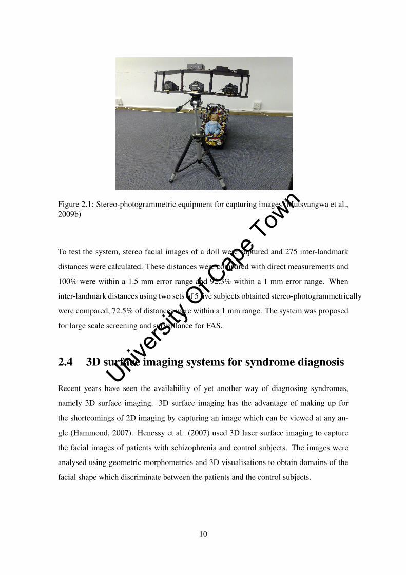
Figure 2.1: Stereo-photogrammetric equipment for capturing images (Mutsvangwa et al.,2009b)
To test the system, stereo facial images of a doll were captured and 275 inter-landmark
distances were calculated. These distances were compared with direct measurements and
100% were within a 1.5 mm error range and 92.3% within a 1 mm error range. When
inter-landmark distances using two sets of 5 live subjects obtained stereo-photogrammetrically
were compared, 72.5% of distances were within a 1 mm range. The system was proposed
for large scale screening and surveillance for FAS.
2.4 3D surface imaging systems for syndrome diagnosis
Recent years have seen the availability of yet another way of diagnosing syndromes,
namely 3D surface imaging. 3D surface imaging has the advantage of making up for
the shortcomings of 2D imaging by capturing an image which can be viewed at any an-
gle (Hammond, 2007). Henessy et al. (2007) used 3D laser surface imaging to capture
the facial images of patients with schizophrenia and control subjects. The images were
analysed using geometric morphometrics and 3D visualisations to obtain domains of the
facial shape which discriminate between the patients and the control subjects.
10
Univers
ity O
f Cap
e Tow
n
Moore et al. (2007) examined 276 subjects from 4 sites (Cape Town, South Africa;
Helsinki, Finland; Buffalo, New York; and San Diego, California) to classify subjects
as either fetal alcohol syndrome positive (FAS; 43%) or control (57%). Facial images
were captured using a commercially available laser scanner. Commercial packages were
used to reconstruct the 3D model of a subject’s face. A discriminant function analysis
was performed on facial measurements obtained from those models to distinguish FAS
patients from controls. It was observed that a reduced size of the eye orbit was a consis-
tent feature discriminating FAS and controls in all populations.
3D photogrammetry can be used to obtain the 3D landmark coordinates of the face as was
demonstrated in (Meintjes et al., 2002; Mutsvangwa et al., 2009b). It can also be used
to reconstruct the craniofacial surface in 3D. As with landmark-based photogrammetry,
multiple digital cameras are used to capture images from different viewing angles but
the craniofacial surface is reconstructed in 3D (Wong et al., 2008). The main advantages
of 3D surface photogrammetry over laser surface scanning is that its data capture time
is very small and hence it minimises motion artifacts. On comparison of a particular
3D surface photogrammetric system (the 3dMD face digital photogrammetry system) to
direct anthropometry, Wong et al. (2008) showed that the 3D system produced results that
were valid and reliable.
2.5 Facial shape analysis for FAS diagnosis
Facial shape can be compared and averaged by analysing the differences in position of
different landmarks as investigated by Clarren et al. (1987) and Streissguth et al. (1991).
These studies were performed by using the mean shapes of triangles defined by three
sets of landmarks on subjects who were either exposed to more alcohol or less alcohol
prenatally.
Mutsvangwa & Douglas (2007) applied Procrustes analysis and principal component
analysis (these methods are described in Chapter 3) to stereo-photogrammetrically ob-
11
Univers
ity O
f Cap
e Tow
n
tained 3D landmarks to analyse the differences in landmark-based facial shapes between
subjects suffering from FAS and those of the normal controls. They found significant
differences in shape between the groups, which confirmed the dysmorphology expected
in FAS subjects.
Mutsvangwa et al. (2009a) described an application of facial shape analysis to charac-
terise the facial anomalies associated with fetal alcohol syndrome (FAS) in a mixed an-
cestry population, in which the influence of size and age on shape was removed by re-
gression. Stereo facial images were acquired using the equipment shown in Figure 2.1
and generalised Procrustes analysis and discriminant function analysis were applied to
3D coordinates. Facial shape comparisons of FAS and control subjects at ages 5 and 12,
a comparison of the FAS facial shape at ages 5 and 12 and a comparison of control facial
shapes at ages 5 and 12 were done. The first two comparisons indicated that the facial fea-
tures which most differentiated between FAS and control were small palpebral fissures,
a thin upper lip and midface hypoplasia. The classification accuracy for the 5-year-old
group was 95.46% while that for the 12-year-old group was 80.13%. The remaining com-
parisons confirmed that the FAS facial anomalies diminish with age.
Using the same shape analysis techniques as in Mutsvangwa and Douglas (2007), Mutsvangwa
(2009) applied classification techniques to the shape information extracted from stereo
images in order to classify the FAS and normal subjects. The results are shown in Table
2.1.
12
Univers
ity O
f Cap
e Tow
n
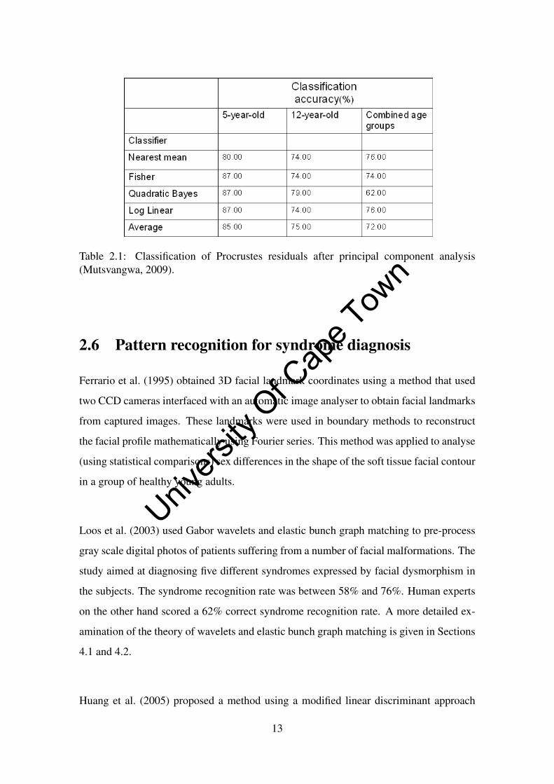
Table 2.1: Classification of Procrustes residuals after principal component analysis(Mutsvangwa, 2009).
2.6 Pattern recognition for syndrome diagnosis
Ferrario et al. (1995) obtained 3D facial landmark coordinates using a method that used
two CCD cameras interfaced with an automatic image analyser to obtain facial landmarks
from captured images. These landmarks were used in boundary methods to reconstruct
the facial profile mathematically using Fourier series. This method was applied to analyse
(using statistical comparisons) sex differences in the shape of the soft tissue facial contour
in a group of healthy young adults.
Loos et al. (2003) used Gabor wavelets and elastic bunch graph matching to pre-process
gray scale digital photos of patients suffering from a number of facial malformations. The
study aimed at diagnosing five different syndromes expressed by facial dysmorphism in
the subjects. The syndrome recognition rate was between 58% and 76%. Human experts
on the other hand scored a 62% correct syndrome recognition rate. A more detailed ex-
amination of the theory of wavelets and elastic bunch graph matching is given in Sections
4.1 and 4.2.
Huang et al. (2005) proposed a method using a modified linear discriminant approach
13
Univers
ity O
f Cap
e Tow
n

(LDA) called the enhanced Fisher model for identifying FAS positive faces using facial
images. The images were cropped and normalised into the region that contains only the
face. The method consisted of two steps. The first projected a face image to a face
subspace via principal component analysis, by selecting the features (pixels) which con-
tributed most to identifying those images of positive FAS subjects. The second step used
LDA to obtain a linear classification. The accuracy of the classifier was 70.0% when 25
principal components were used.
Vollmar et al. (2008) attempted to classify subjects suffering from 1 of 14 facial malfor-
mation syndromes using frontal and side view images. The authors located specific land-
marks on the face and extracted Gabor coefficients at those landmarks. The coefficients
(jets) store texture information of the area under investigation (Section 3.1). They also
extracted 2D coordinates of the facial landmarks from the frontal and side view images.
The texture information and the coordinates were used as features for classification. The
classification methods tested were: linear discriminant analysis, support vector machines
and the k-nearest neighbour classifier. From the results, its was deduced that substantial
information can be obtained from side poses and geometry. The classification accuracy
when investigating 14 syndromes from frontal images and side-views using wavelets was
76% but increased to 93% when geometric information (landmark coordinates) was in-
cluded.
Fang et al. (2008) developed an automated facial feature analysis technique which com-
pared mathematically defined surface features within selected regions of FAS and control
facial surface images, obtained using a laser scanner. It extracted a subset of these fea-
tures which provided the most discriminatory power to identify the FAS subjects. The
feature measurements used in this study were: area, aspect ratio, flatness and curvature.
A correlation-based feature selection approach was used to reduce the size of the feature
vector. The selected feature vector was analysed using radial basis function networks as
well as support vector machines. The study used two different test populations. The ac-
curacy for the first group was 88.2% while for the second group the accuracy for correctly
14
Univers
ity O
f Cap
e Tow
n
classifying FAS was 90.9%.
2.7 Landmark location
Locating facial landmarks on a photograph is an important step in various operations
such as face recognition and classification. The most common way of doing so is to
manually select the facial landmarks by visual inspection. The advantage of this method
is its accuracy, however, the location procedure depends on the experience of the user in
identifying the landmarks. The problem with manual detection of the facial landmarks
arises when a large number of photographs is needed. For this reason, automatic facial
landmark location is ideal when dealing with a dataset of considerable size.
An algorithm, developed by Douglas et al. (2003), was applied to photographs of 46 six
to seven-year-old children. The algorithm uses peak and valley maps and integral projec-
tion functions, to locate the eyes and extract the iris, and genetic algorithms to fit cubic
splines to the upper and lower eyelids. Automatically obtained measurements using this
algorithm were compared with manually obtained measurements from the photographs.
It was found that the mean absolute differences between automatic and manual measure-
ments were less than 1mm for palpebral fissure length (PFL) and interpupillary distance
(IPD).
Elastic bunch graph matching (EBGM) is one technique of automatic landmark detection
which was developed by Wiskott et al. (1999) and has been used for face recognition.
The theory behind EBGM is given in detail in Section 4.2. EBGM uses Gabor wavelets
to store information about the local facial features. EBGM was used by Loos et al. (2003),
Boehringer et al. (2006) and Vollmar et al. (2008) to locate landmarks in digital facial
photographs for the analysis of facial malformations. The studies included classification
exercises to identify the syndromes causing the dysmorphisms.
15
Univers
ity O
f Cap
e Tow
n

Naftel and Trenouth (2004) used a semi-automated approach to 3D landmark digitiza-
tion of the face which uses a combination of active shape model-driven feature detection
and stereo-photogrammetric analysis. A hybrid stereo-photogrammetric and structured-
light imaging system was used for acquiring 3D face models. Landmark-based statistical
analysis of facial shape change was then carried out using Procrustes registration, prin-
cipal component analysis and thin plate spline warping on 2D facial midline profiles and
automatically digitized 3D landmarks. It was shown that the method was capable of dis-
tinguishing between changes in facial morphology due to simulated surgical correction
and changes due to other factors. The study also showed that the proposed method may
be used for evaluating the results of clinical treatment or surgical procedures which result
in changes to facial soft tissue morphology.
Grobbelaar and Douglas (2007) developed an algorithm that automatically found matched
feature points on the second of a pair of stereo images, after manual landmarking of the
first. Palpebral fissure length, interpupillary distance, inner canthal distance and outer
canthal distance, as well as distances that can be used to approximate the circularity of the
upper lip, were obtained from manually marking both images, and automatically marking
the second image. The results showed that the mean differences between manual and
automatic marking were less than 1 mm.
Wang et al. (2008) developed a method which automatically detects and tracks facial
landmarks in videos, and then extracts geometric features to characterise facial expression
changes. A face is detected in the first frame of the video. Once the face has been detected,
58 landmarks which are important to characterise facial features are identified by using
active appearance models (AAM). AAM is a statistical method to model face appearance
as well as facial shape. These methods were applied to healthy controls and case studies
of patients with schizophrenia and Asperger’s syndrome. The results demonstrated the
ability of the video-based expression analysis method in capturing subtleties of facial
expression.
16
Univers
ity O
f Cap
e Tow
n
Chapter 3
Pattern recognition theory
This chapter gives an overview on the theory of Gabor wavelets and jets. The process
of elastic bunch graph matching (EBGM) is then explained. EBGM is used as a face
detection and feature extraction method from facial images. The features extracted in
EBGM are in the form of texture information (jets). Texture information together with
geometry information (2D or 3D coordinates) can be used as features to classify new
faces. Details of various classifiers (k-nearest neighbour, linear discriminant analysis
and support vector machines) are given. Procrustes analysis, which is a shape analysis
method, is also described.
3.1 Wavelets and jets
Loos et al. (2003) and Vollmar et al. (2008) employed a method using Gabor wavelets to
diagnose syndromes associated with dysmorphic faces. Wavelets are functions that satisfy
certain mathematical requirements and are used in representing data or other functions,
similar to sines and cosines in the Fourier transform. However, the wavelet transform
represents data at different scales or resolutions, which distinguishes it from the Fourier
transform (Dai and Yan, 2007).
Gabor wavelets can be described as Gaussian functions modulated by a sinusoidal signal
as described by the equations (Shen and Bai, 2006):
17
Univers
ity O
f Cap
e Tow
n

ϕ(t) = exp(−α2t2)exp(− j2π f0t)
where α is the sharpness of the Gaussian, f0 is the centre frequency of the sinusoidal
signal and j is the complex root of −1.
Gabor wavelets can also be represented in the frequency domain by:
Φ( f ) =√
π
α2 exp(− π2
α2 ( f − f0)2)
Figure 3.1(a) shows how the shapes of the wavelets are decided by the Gaussian sharpness
and are invariant to the frequency. In order to make the sharpness of the Gaussian depen-
dent on the central frequency f0, a constant ratio γ = f0α
is defined so that the functions on
different frequencies behave as scaled versions of each other. The equation now becomes:
ϕ(t) =| f0γ√
πexp(− f 2
0γ2 t2)
exp(− j2π f0t) |
Figure 3.1(b) shows examples of such wavelets.
Figure 3.1: Gabor functions of (a) fixed Gaussian shapes and (b) varied Gaussian shapes(Shen and Bai, 2006).
Wavelets can also be represented in 3D as shown in Figure 3.2 :
18
Univers
ity O
f Cap
e Tow
n
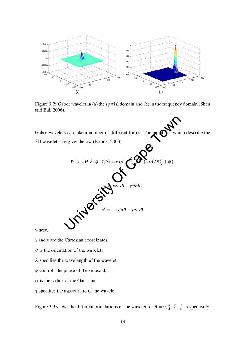
Figure 3.2: Gabor wavelet in (a) the spatial domain and (b) in the frequency domain (Shenand Bai, 2006).
Gabor wavelets can take a number of different forms. The equations which describe the
3D wavelets are given below (Bolme, 2003):
W (x,y,θ ,λ ,φ ,σ ,γ) = exp(−x′2+γ2y′2
2σ2 )cos(2πx′λ
+φ),
x′ = xcosθ + ysinθ ,
y′ =−xsinθ + ycosθ
where,
x and y are the Cartesian coordinates,
θ is the orientation of the wavelet,
λ specifies the wavelength of the wavelet,
φ controls the phase of the sinusoid,
σ is the radius of the Gaussian,
γ specifies the aspect ratio of the wavelet.
Figure 3.3 shows the different orientations of the wavelet for θ = 0, π
4 , π
2 , 3π
4 , respectively.
19
Univers
ity O
f Cap
e Tow
n
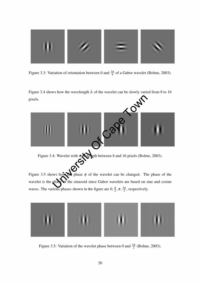
Figure 3.3: Variation of orientation between 0 and 3π
4 of a Gabor wavelet (Bolme, 2003).
Figure 3.4 shows how the wavelength λ of the wavelet can be slowly varied from 8 to 16
pixels.
Figure 3.4: Wavelet with wavelength between 8 and 16 pixels (Bolme, 2003).
Figure 3.5 shows how the phase φ of the wavelet can be changed. The phase of the
wavelet is the phase of the sinusoid since Gabor wavelets are based on sine and cosine
waves. The various phases shown in the figure are 0, π
2 ,π, 3π
2 , respectively.
Figure 3.5: Variation of the wavelet phase between 0 and 3π
2 (Bolme, 2003).
20
Univers
ity O
f Cap
e Tow
n
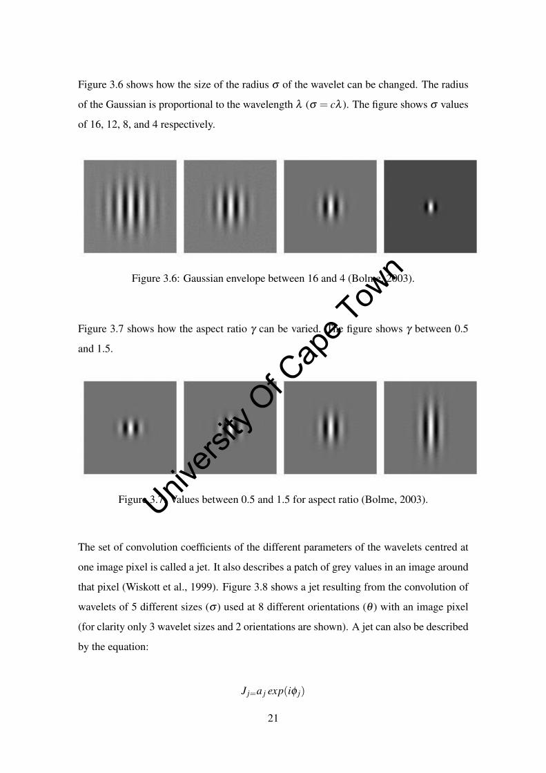
Figure 3.6 shows how the size of the radius σ of the wavelet can be changed. The radius
of the Gaussian is proportional to the wavelength λ (σ = cλ ). The figure shows σ values
of 16, 12, 8, and 4 respectively.
Figure 3.6: Gaussian envelope between 16 and 4 (Bolme, 2003).
Figure 3.7 shows how the aspect ratio γ can be varied. The figure shows γ between 0.5
and 1.5.
Figure 3.7: Values between 0.5 and 1.5 for aspect ratio (Bolme, 2003).
The set of convolution coefficients of the different parameters of the wavelets centred at
one image pixel is called a jet. It also describes a patch of grey values in an image around
that pixel (Wiskott et al., 1999). Figure 3.8 shows a jet resulting from the convolution of
wavelets of 5 different sizes (σ ) used at 8 different orientations (θ ) with an image pixel
(for clarity only 3 wavelet sizes and 2 orientations are shown). A jet can also be described
by the equation:
J j=a j exp(iφ j)
21
Univers
ity O
f Cap
e Tow
n

where a j is the magnitude of the jet and φ j is the phase.
Figure 3.8: Example of a jet (Loos et al., 2003).
2D facial images can be represented by image graphs. This is done by convolving the fa-
cial images, at the location of selected landmarks on the facial image, with Gabor wavelets
of different parameters. In this way, each landmark of the facial image is represented by
a jet in an image graph. The convolution coefficients (jets) at each landmark describe a
small patch of gray values around that region. Each landmark is referred to as a node, and
each node is connected to another node by an edge. This is illustrated in Figure 3.9.
Figure 3.9: Example of an image graph with 9 nodes and 13 edges (Wiskott et al., 1999).
22
Univers
ity O
f Cap
e Tow
n
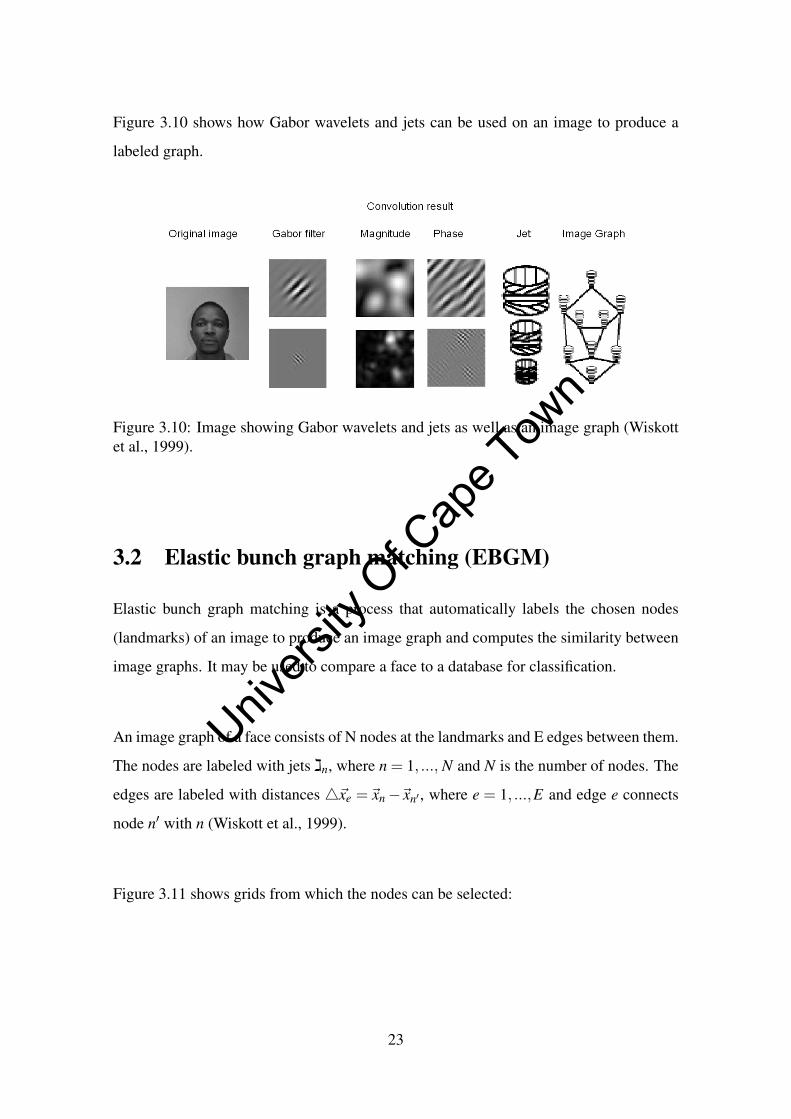
Figure 3.10 shows how Gabor wavelets and jets can be used on an image to produce a
labeled graph.
Figure 3.10: Image showing Gabor wavelets and jets as well as an image graph (Wiskottet al., 1999).
3.2 Elastic bunch graph matching (EBGM)
Elastic bunch graph matching is a process that automatically labels the chosen nodes
(landmarks) of an image to produce an image graph and computes the similarity between
image graphs. It may be used to compare a face to a database for classification.
An image graph of a face consists of N nodes at the landmarks and E edges between them.
The nodes are labeled with jets ,nג where n = 1, ..., N and N is the number of nodes. The
edges are labeled with distances 4~xe =~xn−~xn′ , where e = 1, ...,E and edge e connects
node n′ with n (Wiskott et al., 1999).
Figure 3.11 shows grids from which the nodes can be selected:
23
Univers
ity O
f Cap
e Tow
n
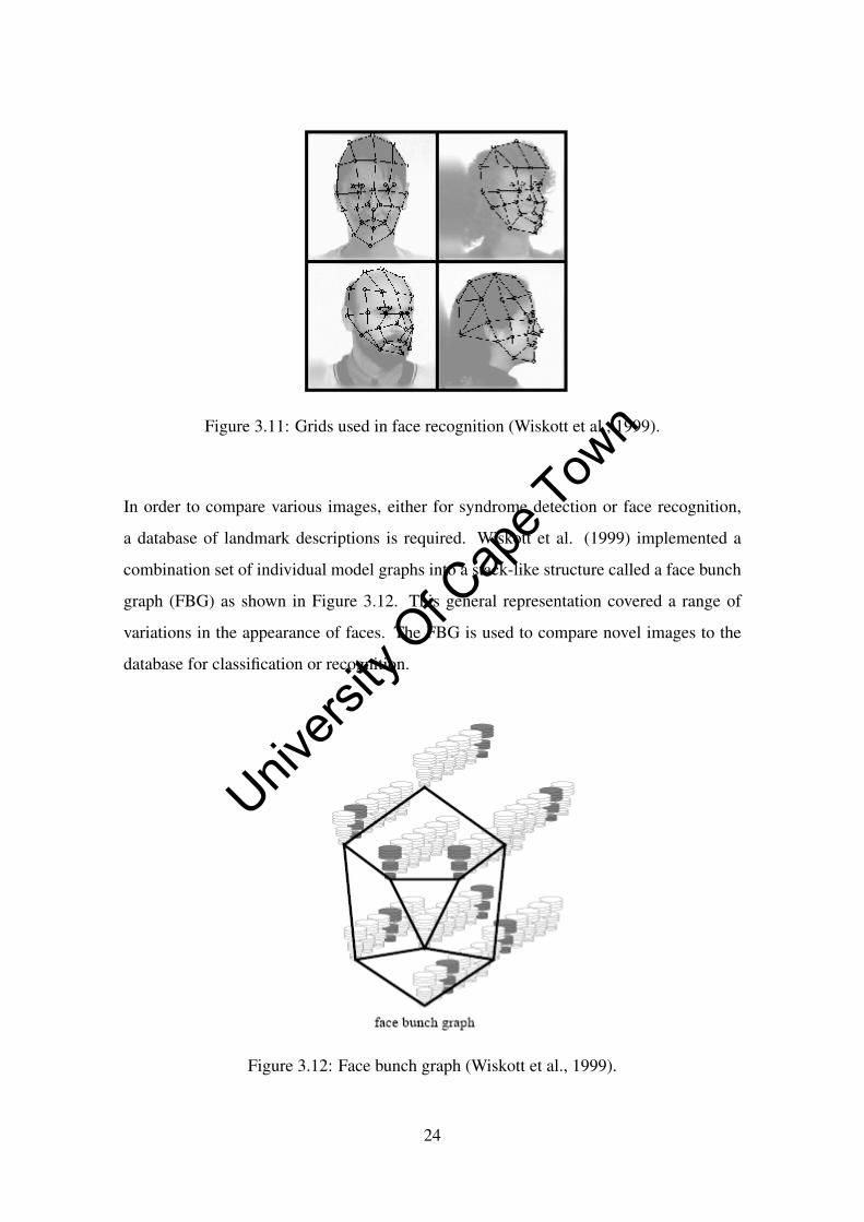
Figure 3.11: Grids used in face recognition (Wiskott et al., 1999).
In order to compare various images, either for syndrome detection or face recognition,
a database of landmark descriptions is required. Wiskott et al. (1999) implemented a
combination set of individual model graphs into a stack-like structure called a face bunch
graph (FBG) as shown in Figure 3.12. This general representation covered a range of
variations in the appearance of faces. The FBG is used to compare novel images to the
database for classification or recognition.
Figure 3.12: Face bunch graph (Wiskott et al., 1999).
24
Univers
ity O
f Cap
e Tow
n

Each of the models have the same grid structure and the nodes correspond to identical
landmarks. Each node is represented by a set of jets which is called a bunch.
The EBGM algorithm computes the similarity of two images. To do so, it applies a Gabor
wavelet convolution to the landmark location or node of a particular facial feature (such as
the nose tip, the eye and mouth) on an image to extract information about the feature (as
a jet). A face graph is constructed after locating all the landmarks required. Two images
can be compared using a similarity function which computes the similarities of the jets in
the face graphs.
3.2.1 Jet similarity function
Jets can be compared using two types of similarity functions, one ignoring the phase
component of jets and one which takes the phase into account. The following equation
describes the similarity function between jets J and J′ which ignores the phase (Wiskott
et al., 1999):
Sa(J,J′) =∑ja ja′j√
∑ja2
j ∑ja′2j
with a and a′ being their magnitudes respectively. The phase sensitive function is given
as shown:
Sφ (J,J′) =∑ja ja′jcos(φ j−φ ′j−~d~k j)√
∑ja2
j ∑ja′2j
where φ j and φ ′j are the phase components and ~d is the small displacement vector between
the two jets and ~k j is the spatial frequency of the kernels.
3.2.2 Displacement estimation
To estimate the displacement vector ~d = (dx,dy) a method used for disparity estimation
is used. The aim is to maximise the similarity Sφ in its Taylor expansion (Wiskott et al.,
25
Univers
ity O
f Cap
e Tow
n

1999):
Sφ (J,J′) =∑ja ja′j[1−0.5(φ j−φ ′j−~d~k j)2]√
∑ja2
j ∑ja′2j
Setting ∂
∂dxSφ = ∂
∂dySφ = 0 and solving for ~d leads to
~d(J,J′) =(
dxdy
)= 1
ΓxxΓyy−ΓxyΓyx×
Γyy −Γyx
−Γxy Γxx
(ΦxΦy
),
if ΓxxΓyy−ΓxyΓyx 6= 0, with
Φx = ∑ja ja′jk jx
(φ j−φ ′j
),
Γxy = ∑ja ja′jk jxk jy
and Φy,Γxx,Γyx,Γyy defined correspondingly.
3.2.3 Matching procedure
The goal of EBGM on a new image is to automatically find the landmarks and hence
extract a face graph so that it can be compared to the database. The matching process
consists of 4 steps (Wiskott et al., 1999):
1. Find approximate face position. Condense the face bunch graph (FBG) into an
average graph by taking the average magnitude of the jets in each bunch of the
FBG. This is used as a rigid model. Evaluate its similarity to the input image at
each location of a square lattice with a spacing of 4 pixels. At this step the similarity
function Sa without phase is used. The scanning is repeated around the best fitting
position with a spacing of 1 pixel. The best fitting position serves as the starting
point for the next step.
2. Refine position and size. The FBG is now used without averaging, varying it in
position and size. Check the four different positions ([±3,±3] pixels) displaced
from the position found in Step 1, and at each position check two different sizes
26
Univers
ity O
f Cap
e Tow
n

which have the same centre position. For each of these eight variations, the best
fitting jet for each node or landmark is selected and its displacement (see Section
4.2.2) is computed. The grids are then rescaled and repositioned to minimise the
square sum over the displacements. The best of the eight variations are retained for
the next step.
3. Refine size and find aspect ratio. A similar relaxation process as described for Step
2 is applied but relaxing the x− and y− dimensions independently.
4. Local distortion. By applying a pseudo-random sequence, the position of each
individual image node is varied to further increase the similarity to the FBG. In
this step, only those positions are considered for which the estimated displacement
vector is small.
3.2.4 Graph information
The steps described in Sections 3.2.1, 3.2.2 and 3.2.3 form part of the EBGM operation.
The graph obtained after EBGM contains information about the landmarks and their sur-
roundings. The nodes are labeled with jets. A jet contains local texture information and
is calculated with a set of Gabor wavelets as described in Section 3.1. The nodes are
connected by edges and these edges code the topology between the nodes. Hence the
2D information of the landmarks is also inherently stored in an image graph. The jets
together with the geometry information can be used for classification at a later stage.
3.3 Generalised Procrustes analysis
The shape of an object can be defined as all the geometrical information that remains
when location, scale and rotational effects are eliminated. Two shapes can be compared
by adjusting for size and superimposing one shape on the other (Dryden and Mardia,
1998). Any differences remaining are attributed to the differences in shape. Morpho-
metrics is the study of shape variation and its covariation with other variables. Tradi-
27
Univers
ity O
f Cap
e Tow
n
tionally, morphometrics was the application of multivariate statistical analyses to sets of
quantitative variables such as length, width, and height (Adams et al., 2004). Traditional
morphometrics made use of linear distance measurements and often included counts, ra-
tios and angles. The covariation in the morphological measurements could be quantified
and the patterns of variation could be assessed. However, owing to the correlation of lin-
ear distance measurements with size, size-free shape variables could not be extracted for
analysis. Because of these shortcomings, it was necessary to explore alternative methods
which captured the geometry of morphological structure for both outline and landmark
data. A ‘new’ method called geometric morphometrics was suggested. Superimposition
methods aid in removing non-shape variation in configurations of landmarks by an opti-
mised method of overlaying them. One such method is the generalised Procrustes anal-
ysis (GPA) which superimposes landmark configurations using least-square estimates for
translation and rotation parameters (Adams et al., 2004). Optimum superposition of shape
objects is achieved when translation and rotation effects are adjusted so as to minimise
the distances between landmarks (Halazonetis, 2004). The process of landmark-based
morphometrics starts with the collection of 2D or 3D coordinates.
An n -point/landmark shape in k -dimensions can be mathematically represented by con-
catenating each dimension into a (kxn) vector. The Procrustes method is used to fit all
n landmarks for N objects with optimal superimposing of landmarks (Rohlf and Slice,
1990). The method also minimises the sum of the squared distances between correspond-
ing points (Halazonetis, 2004). The process of superimposition of 2 shapes is described
below (Mutsvangwa, 2009):
1. The centroid size of each shape is calculated (i.e, the centre of gravity of the shape).
2. Each shape is normalised by dividing by the centroid size.
3. The shapes are aligned with respect to position at their centroids.
4. Each shape is then realigned with respect to rotational orientation about their cen-
troids.
28
Univers
ity O
f Cap
e Tow
n
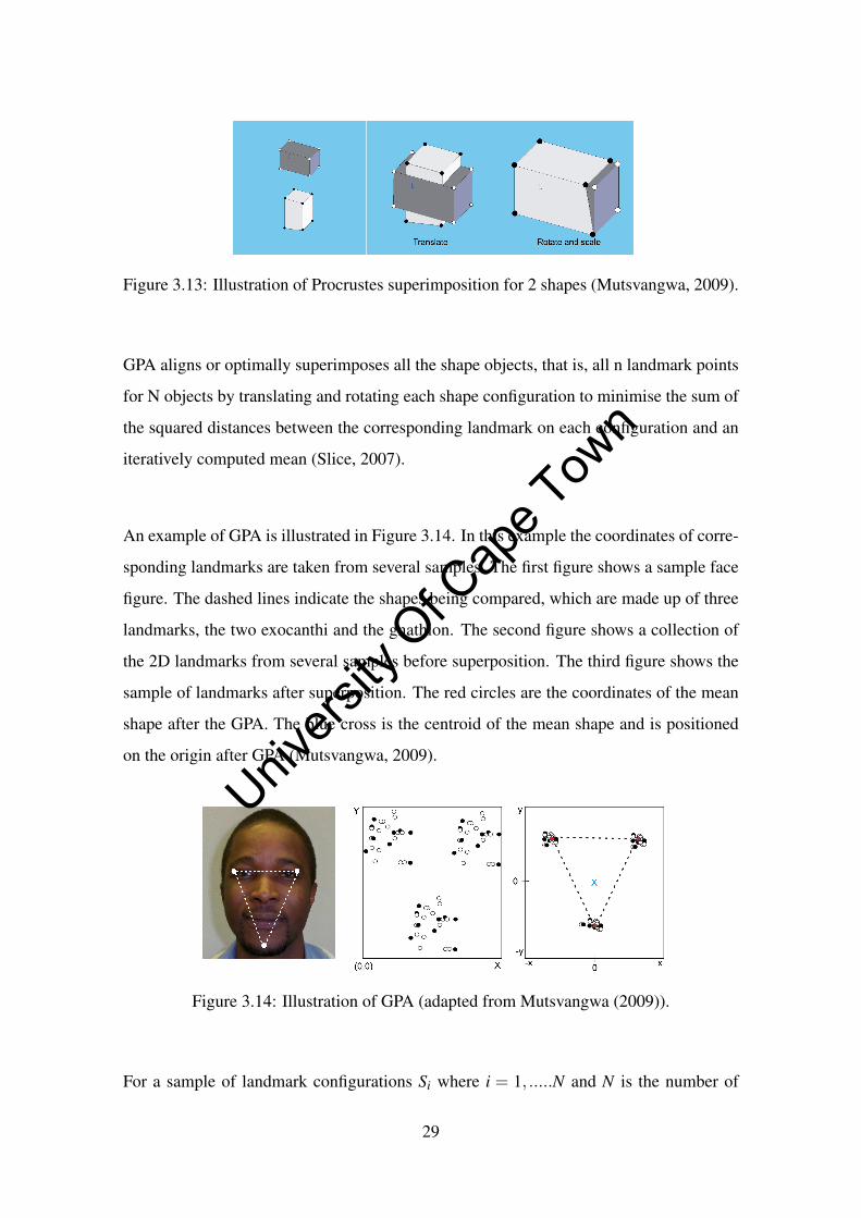
Figure 3.13: Illustration of Procrustes superimposition for 2 shapes (Mutsvangwa, 2009).
GPA aligns or optimally superimposes all the shape objects, that is, all n landmark points
for N objects by translating and rotating each shape configuration to minimise the sum of
the squared distances between the corresponding landmark on each configuration and an
iteratively computed mean (Slice, 2007).
An example of GPA is illustrated in Figure 3.14. In this example the coordinates of corre-
sponding landmarks are taken from several samples. The first figure shows a sample face
figure. The dashed lines indicate the shapes being compared, which are made up of three
landmarks, the two exocanthi and the gnathion. The second figure shows a collection of
the 2D landmarks from several samples before superposition. The third figure shows the
sample of landmarks after superposition. The red circles are the coordinates of the mean
shape after the GPA. The blue cross is the centroid of the mean shape and is positioned
on the origin after GPA (Mutsvangwa, 2009).
Figure 3.14: Illustration of GPA (adapted from Mutsvangwa (2009)).
For a sample of landmark configurations Si where i = 1, .....N and N is the number of
29
Univers
ity O
f Cap
e Tow
n
specimens, α , the Procrustes mean shape after convergence can be estimated by:
α =1N
N
∑i=1
αi
and gives the Procrustes mean coordinates (α jx,α jy,α jz,) where j = 1, ...n (n is the number
of landmarks). The full Procrustes fit coordinates SPi are found by fitting each shape Si to
the Procrustes mean α using most commonly a least-squares method (Halazonetis, 2004).
Therefore each Procrustes fit SPi has coordinates (SP
i jx, SP
i jy, SP
i jz,). Procrustes residuals SPR
i
are the difference between the full Procrustes fit coordinates and the Procrustes mean co-
ordinates and are denoted by (SPRi jx
, SPRi jy
, SPRi jz
,) (Robinson et al., 2001). Procrustes residuals
have properties which may be useful for statistical analysis (McIntyre and Mossey, 2003).
3.4 Classification methods
Given a query vector (object) x0 and a set of N labeled instances xi,yiN1 , the task of
the classifier is to predict the class label of x0 on the predefined P classes. An object is a
k-dimensional vector of feature value or class membership. Each object has the same set
of features with different values and this is called the feature space.
3.4.1 K-Nearest Neighbour
The k-nearest neighbor (kNN) classification algorithm tries to find the k nearest neighbors
of x0 and uses a majority vote to determine the class label of x0. Without prior knowledge,
the kNN classifier usually applies Euclidean distances as the distance metric (Song et al.,
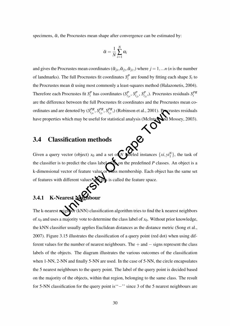
2007). Figure 3.15 illustrates the classification of a query point (red dot) when using dif-
ferent values for the number of nearest neighbours. The + and− signs represent the class
labels of the objects. The diagram illustrates the various outcomes of the classification
when 1-NN, 2-NN and finally 5-NN are used. In the case of 5-NN, the circle encapsulates
the 5 nearest neighbours to the query point. The label of the query point is decided based
on the majority of the objects, within that region, belonging to the same class. The result
for 5-NN classification for the query point is‘‘−’’ since 3 of the 5 nearest neighbours are
30
Univers
ity O
f Cap
e Tow
n
of the ‘‘−’’ class.
Figure 3.15: Example of a 2D kNN classification problem (StatSoft, 1984-2008a).
3.4.2 Linear discriminant analysis
Discriminant analysis is a statistical technique which allows for the study of differences
between two or more groups of objects with respect to several variables simultaneously
(Klecka, 1980). Linear discriminant analysis (LDA) finds a linear transformation of the
variables which improves the discriminative power of the variables. There are different
approaches to classification using LDA (Balakrishnama and Ganapathiraju, 1998). These
modifications of LDA are given by:
• Class dependent transformation which maximises the ratio of between-class vari-
ance to within-class variance.
• Class independent transformation which maximises the ratio of overall variance to
within-class variance.
Typically, class-dependent transformation is used, in which the optimisation criterion
maximises the ratio of between-class variance to within-class variance. The solution ob-
tained by maximising this criterion defines the axes of a transformed space. A transfor-
mation is done by projecting the data onto the new set of axes which have been rotated in
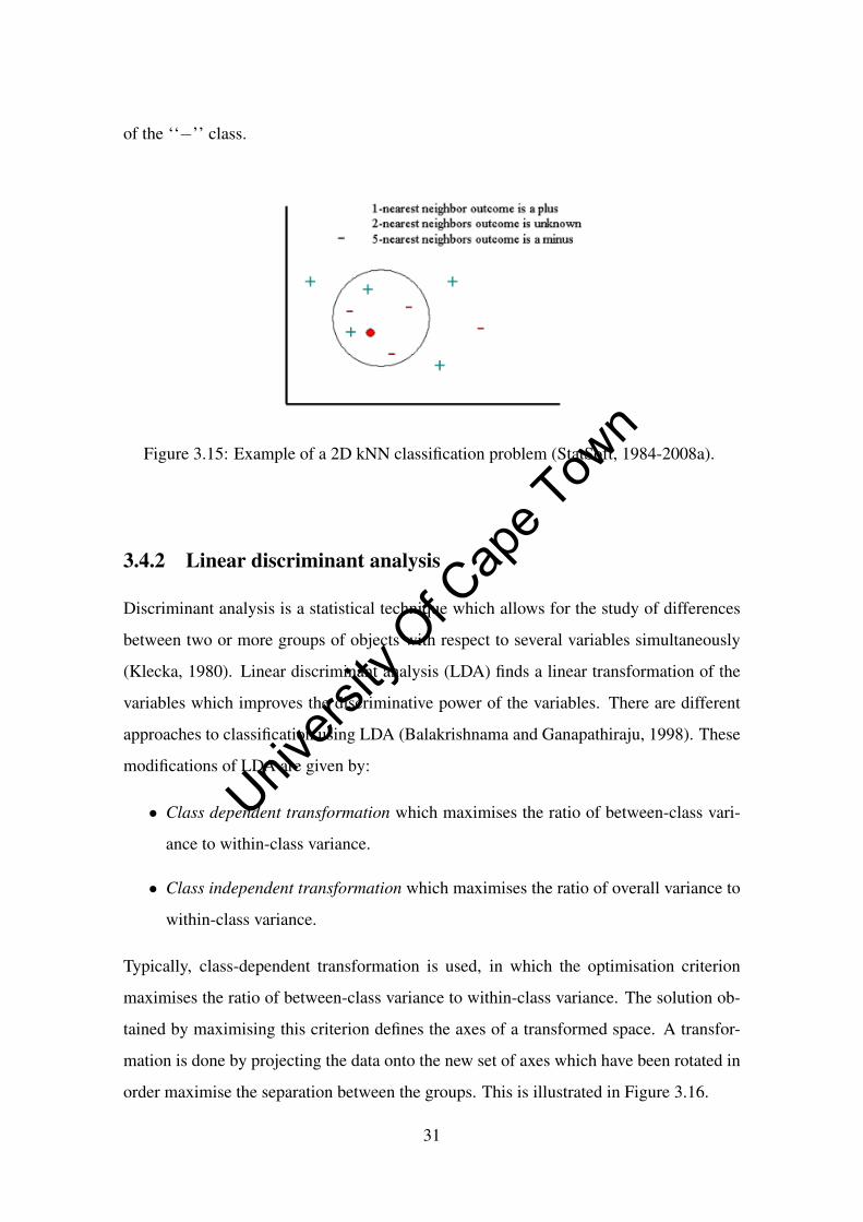
order maximise the separation between the groups. This is illustrated in Figure 3.16.
31
Univers
ity O
f Cap
e Tow
n
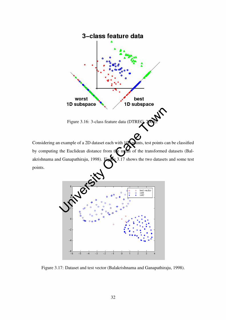
Figure 3.16: 3-class feature data (DTREG, 2003).
Considering an example of a 2D dataset each with 100 points, test points can be classified
by computing the Euclidean distance from the mean of the transformed datasets (Bal-
akrishnama and Ganapathiraju, 1998). Figure 3.17 shows the two datasets and some test
points.
Figure 3.17: Dataset and test vector (Balakrishnama and Ganapathiraju, 1998).
32
Univers
ity O
f Cap
e Tow
n
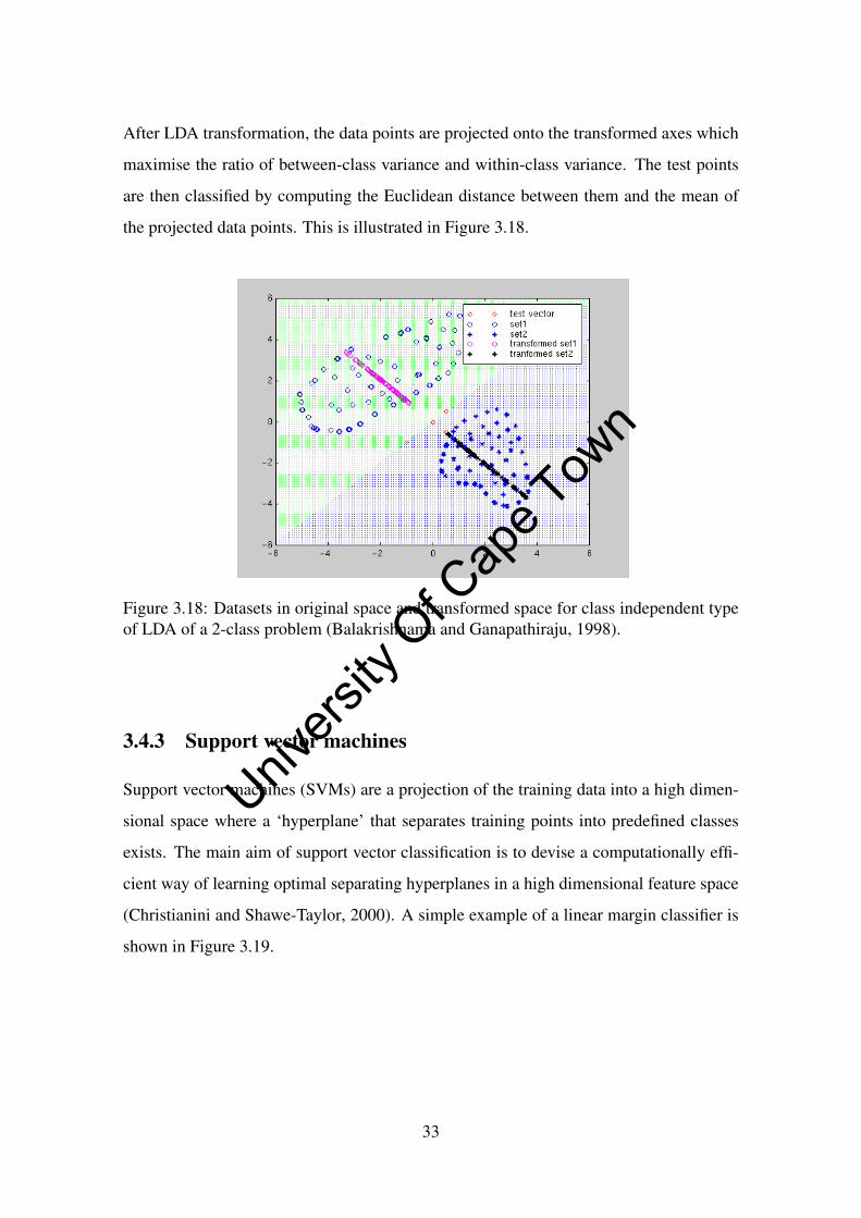
After LDA transformation, the data points are projected onto the transformed axes which
maximise the ratio of between-class variance and within-class variance. The test points
are then classified by computing the Euclidean distance between them and the mean of
the projected data points. This is illustrated in Figure 3.18.
Figure 3.18: Datasets in original space and transformed space for class independent typeof LDA of a 2-class problem (Balakrishnama and Ganapathiraju, 1998).
3.4.3 Support vector machines
Support vector machines (SVMs) are a projection of the training data into a high dimen-
sional space where a ‘hyperplane’ that separates training points into predefined classes
exists. The main aim of support vector classification is to devise a computationally effi-
cient way of learning optimal separating hyperplanes in a high dimensional feature space
(Christianini and Shawe-Taylor, 2000). A simple example of a linear margin classifier is
shown in Figure 3.19.
33
Univers
ity O
f Cap
e Tow
n
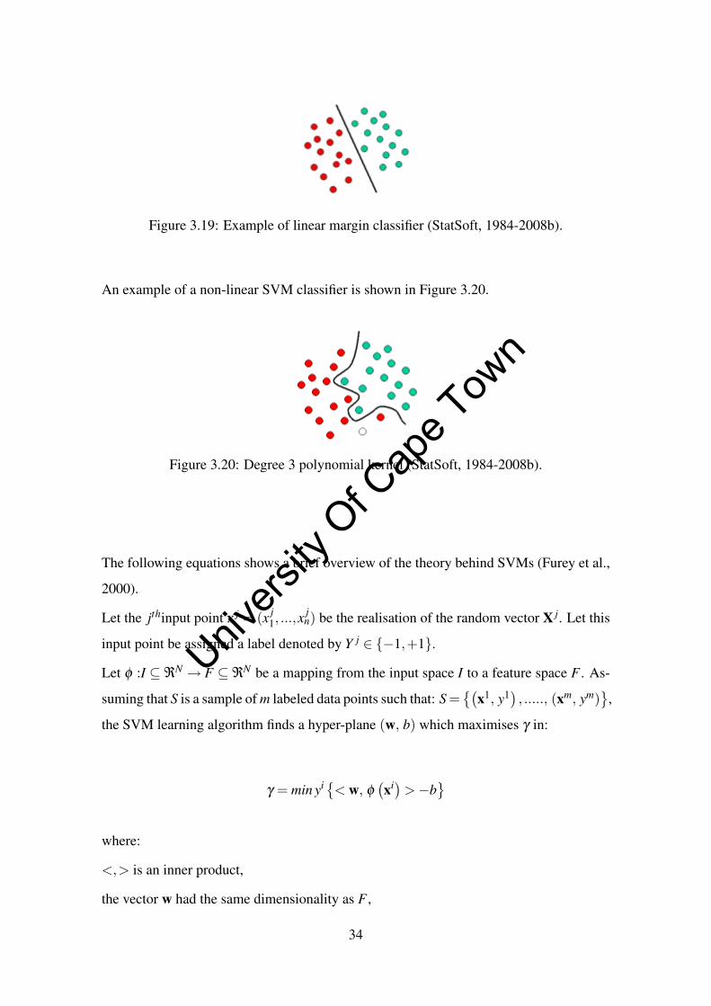
Figure 3.19: Example of linear margin classifier (StatSoft, 1984-2008b).
An example of a non-linear SVM classifier is shown in Figure 3.20.
Figure 3.20: Degree 3 polynomial kernel (StatSoft, 1984-2008b).
The following equations shows a brief overview of the theory behind SVMs (Furey et al.,
2000).
Let the jthinput point x j = (x j1, ...,x
jn) be the realisation of the random vector X j. Let this
input point be assigned a label denoted by Y j ∈ −1,+1.
Let φ :I ⊆ℜN → F ⊆ℜN be a mapping from the input space I to a feature space F . As-
suming that S is a sample of m labeled data points such that: S =(
x1, y1) , ....., (xm, ym)
,
the SVM learning algorithm finds a hyper-plane (w, b) which maximises γ in:
γ = min yi< w, φ(xi)>−b
where:
<,> is an inner product,
the vector w had the same dimensionality as F ,
34
Univers
ity O
f Cap
e Tow
n

‖ w ‖is held constant,
b is a real number and
γ is the margin.
The quantity(< w, φ
(xi)>−b
)corresponds to the distance between the point xi and
the decision boundary. When it is multiplied by yi it either gives a positive value for a
correct classification or a negative value for incorrect ones. Given a unknown data point
x, a label is assigned to it depending on its relationship to the decision boundary. The
decision function is given by:
f (x) = sign(< w, φ (x) >−b)
3.4.4 Feature selection using principal component analysis
Classification using a large number of features can lead to a common problem known as
the ‘curse of dimensionality’. Working with a large number of features with respect to the
number of subjects adversely affects the classification accuracy (Janecek and Gansterer,
2008). Working in lower dimensions yields less complex classifiers and hence better
generalisations can be obtained.
Therefore principal component analysis can be used to reduce the dimensionality of the
database before attempting any classification methods. Each subject and their features are
stored in the format which follows (Yambor, 2000).
xi =[xi
1 . . . xiN]T
i = number of subjects,
N = number of features,
T here means that the vector is transposed.
The mean of all subjects is subtracted from the individual subject as follows:
35
Univers
ity O
f Cap
e Tow
n

xi =[xi−m
], where m =
1P
P
∑i=1
xi
P = number of subjects
The vectors of the subject features are then grouped together to form a matrix.
X =[x1 x2 . . . xP]
X is the database.
The covariance matrix is then calculated by:
Ω = XXT
The eigenvalues and corresponding eigenvectors are found by solving for:
ΩV = hV
where,
V = eigenvectors,
h = eigenvalues
The eigenvectors are then sorted according to their corresponding eigenvalues. Only those
eigenvectors corresponding to non-zero eigenvalues and sometimes other criteria, are re-
tained. These eigenvectors are known as the principal components (PCs). As will be seen
in Section 3.4.4, the PC selection operation can be modified to optimise the classification
accuracy.
The eigenvectors represent the eigenspace onto which the original data can be projected.
36
Univers
ity O
f Cap
e Tow
n
In other words, the eigenvectors are the new axes of the data being investigated. The
vectors are grouped as shown:
V = [v1 v2 . . .vm]
where,
m = the number of eigenvectors retained
To project the original data to eigenspace
X = V T X
where,
X = the projected data
Thus the same dataset can be represented in a subspace with fewer dimensions than it
originally had. A reduced dimensionality implies that there are fewer features to be clas-
sified. Hence PCA can be regarded here as a feature selection scheme.
3.4.5 Leave-one-out cross-validation
Cross-validation is often used to estimate the generalisation ability of a statistical clas-
sifier (that is, the performance on previously unseen data). Under cross-validation, the
available data is divided into k disjoint sets; k models are then trained, each on a different
combination of k− 1 partitions and tested on the remaining partition. The most extreme
form of cross-validation, where k is equal to the number of training patterns, is known
as leave-one-out cross-validation. Cross-validation thus makes good use of the available
data as each pattern is used both as training and test data (Cawley and Talbot, 2003).
37
Univers
ity O
f Cap
e Tow
n
Chapter 4
Methods
Two methods are used for extracting image features for classifying faces as having the
FAS facial phenotype, namely elastic bunch graph matching and generalised Procrustes
analysis. This chapter gives details about the study population and how the various fea-
tures (jet information, 2D and 3D coordinates) are extracted. It explains how the database
used for classification is built. The implementation of the classifiers is explained and the
different experiments performed on the database are described.
4.1 Facial landmarks
Several facial features contribute to the unique facial phenotype of FAS, which is mainly
defined by the contraction of the middle third of the face with resultant shortened palpe-
bral fissures, flattened nasal bridge, shortened and upturned nose, smooth philtrum, and
thin upper lip. These features have been emphasized in clinical diagnoses since they
are the only aspect of the syndrome that is specific to FAS (Meintjes et al., 2002). The
anatomical landmarks which aid in analysing these features are shown in Figure 4.1.
38
Univers
ity O
f Cap
e Tow
n

Figure 4.1: Landmarks used on the frontal view . 1. exR - right exocanthion, 2. enR -right endocnathion, 3. g - glabella, 4. n - nasion, 5. se - sellion, 6. enL - left endocanthion,7. exL - left exocanthion, 8. psn - pronasale, 9. alR - right alare, 10. alL - left alare 11.sbalR - right subalare, 12. s - subnasale, 13. sbalL - left sub alare, 14. Phl - centre ofphiltrum furrow, 15. chR - right cheilion, 16. ls’R - right crista philtri, 17. ls - labilaesuperius, 18. ls’L - left crista philtri, 19. chL - left cheilion, 20. li - labiale inferius, 21.umeR - right upper mid eye ridge, 22. umeR - right lower mid eye ridge, 23 umeL - leftupper mid eye ridge, 24. umeL - left lower mid eye ridge, 25. phmR - mid right philtrumridge, 26. PhmL - mid left philtrum ridge, 27. right pupil centre, 28. left pupil centre, 29.tr - trichion and 30. pg - pogonion .
4.2 Study population
4.2.1 Dataset 1
Although the sample size of dataset 1 is relatively small, the same subjects were used in
a study by Mutsvangwa (2009) and Mutsvangwa et al. (2009a) described in Section 2.5.
The use of this dataset allows comparison of the results of the present study to those of the
previous studies. The study population consisted of thirty-four subjects, divided into two
age groups of 5 and 12-years-old. The subjects were of mixed ancestry. These subjects
were part of a larger population of children whose pictures were taken during a large-
scale FASD screening program in the Northern Cape Province of South Africa. Those
39
Univers
ity O
f Cap
e Tow
n

exhibiting signs of growth retardation based on height, weight and head circumference
were evaluated by a dysmorphologist for FAS. A FAS diagnosis was confirmed by the
presence of substantial facial dysmorphology, by the subject being approximately two
standard deviations below the mean on either verbal or non-verbal intelligence quotient
tests, by the subject exhibiting behavioural problems as measured by the Personal Check-
List (PBCL-36) and by the subject having confirmation of prenatal alcohol exposure. The
PBCL-36 is a scale that measures the behavioural characteristics of FAS, irrespective of
age, race, sex, or intelligence quotient, consisting of 36 items regarding several areas
of functioning: academic performance, social skills and interactions, bodily functions,
communication and speech, personal manner, emotions, and motor skills (May et al.,
2007).
Table 4.1 shows the age-related statistics of the subjects.
Table 4.1: Age-related statistics (in years) of subjects in dataset 1.
4.2.2 Dataset 2
The images of 40 subjects were acquired during a FAS screening program in the Western
Cape Province of South Africa, in which the author participated. The subjects were exam-
ined using the same criteria as those described in Section 4.2.1. The age-related statistics
are shown in Table 4.2. The subjects were of mixed ancestry.
40
Univers
ity O
f Cap
e Tow
n

Table 4.2: Age-related statistics (in years) of subjects in dataset 2.
4.3 Image acquisition
Images were acquired using the stereo-photogrammetry imaging equipment shown in Fig-
ure 2.1 (Mutsvangwa et al., 2009b) and described in Section 2.3.2. Three high-resolution
Canon 350D Digital SLR with 18-55mm variable lens were used to capture images. Each
produces an 8 mega-pixel image with a resolution of 3450 (width) by 2304 (height) pixels.
Images taken were in the CR2 format (proprietary to Canon). The Canon Utilities soft-
ware was used to convert the images into grayscale ‘PNG’ format of 600 x 400 pixels.
This format was chosen for compatibility with the requirements of the EBGM software.
4.4 Methods of analysis
The study combines different methods used in previous studies and applies them to the
two datasets described in Section 4.2.
Sokol et al. (1991) identified several landmarks and their 2D coordinates on frontal and
side view facial images which were used in stepwise discriminant analyses to identify
features which most separated FAS from normal subjects.
Elastic bunch graph matching (EBGM) was used by Loos et al. (2003) and Vollmar et al.
(2008) on facial images of subjects suffering from various facial malformation syndromes.
The aim of the investigations was to classify the different syndromes using wavelets and
41
Univers
ity O
f Cap
e Tow
n
jets. The inclusion of geometric information (Cartesian coordinates of landmarks) in the
study was shown to increase the accuracy of classification.
Mutsvangwa & Douglas (2007) and Mutsvangwa (2009) obtained 3D coordinates of fa-
cial landmarks from stereo-photogrammetrically acquired images. Procrustes analysis
was applied to these coordinates to obtain Procrustes residuals which, after principal com-
ponent analysis, were used to analyse the differences between FAS and normal subjects.
The above progression in features for classification from 2D coordinates alone (Sokol
et al., 1991), to 2D coordinates and texture (Loos et al., 2003; Boehringer et al., 2006;
Vollmar et al., 2008), to 3D information in the form of Procrustes residuals (Mutsvangwa,
2009; Mutsvangwa et al., 2009a) is represented in this study. A further advance is achieved
with the use of 3D information and texture as features for classification. 2D coordinates
are not classified on their own.
The study uses EBGM to extract texture information (in form of jets) and 2D coordinates
from frontal images acquired stereo-photogrammetrically. The jets and 2D coordinates
are used as features in classification of FAS and control subjects. To investigate the
performance of the classification methods when 3D information is combined with jets,
Procrustes residuals are obtained from 3D coordinates of facial landmarks. The 2D co-
ordinates are replaced by Procrustes residuals and classification accuracies for features
consisting of jets and Procrustes residuals are assessed.
4.4.1 EBGM software and 2D feature extraction
The elastic bunch graph matching software used was obtained during a visit to the Institut
für Neuroinformatik, Ruhr-Universität Bochum, Germany. As mentioned in Section 3.2,
EBGM detects a face in a new image, labels the landmarks as nodes and connects these
nodes with edges. The frontal view pictures of the subjects were used during this experi-
ment. The first step is to manually label a few sample images with the desired nodes and
42
Univers
ity O
f Cap
e Tow
n
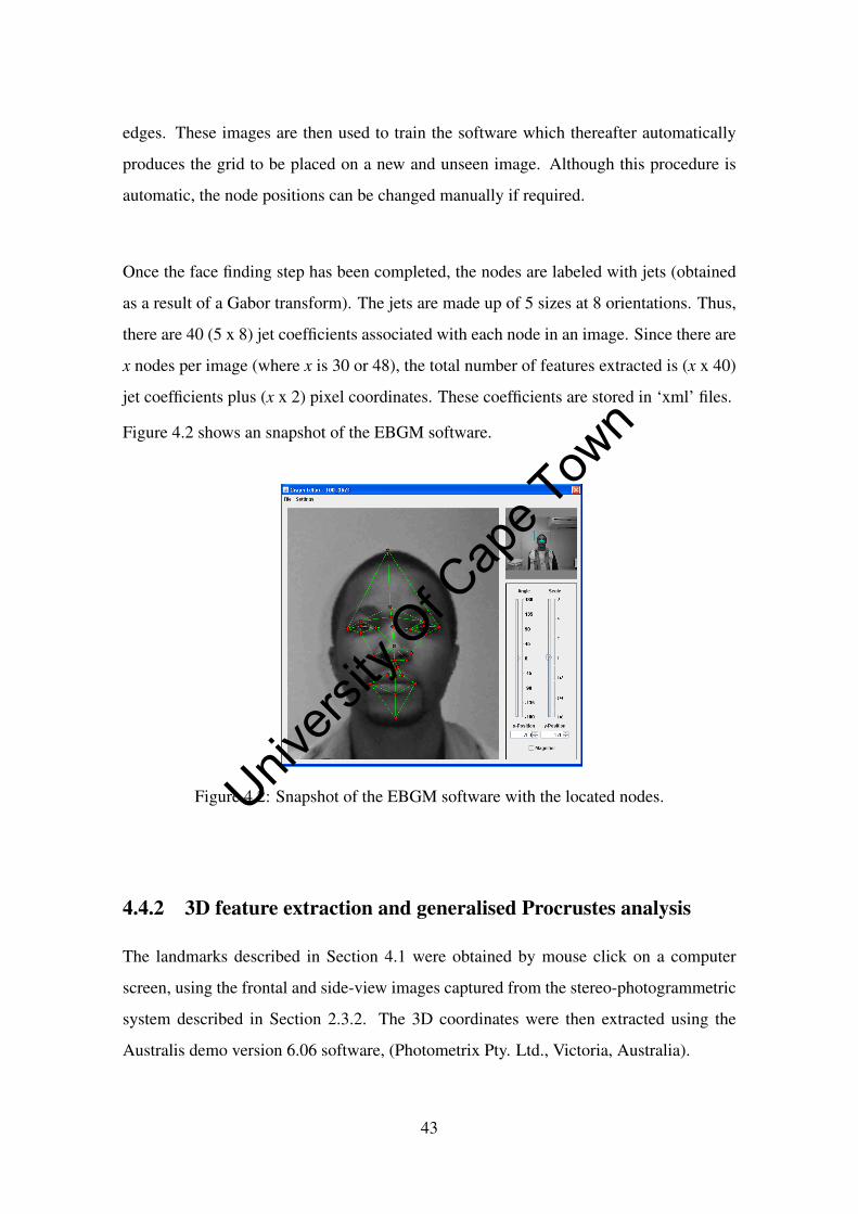
edges. These images are then used to train the software which thereafter automatically
produces the grid to be placed on a new and unseen image. Although this procedure is
automatic, the node positions can be changed manually if required.
Once the face finding step has been completed, the nodes are labeled with jets (obtained
as a result of a Gabor transform). The jets are made up of 5 sizes at 8 orientations. Thus,
there are 40 (5 x 8) jet coefficients associated with each node in an image. Since there are
x nodes per image (where x is 30 or 48), the total number of features extracted is (x x 40)
jet coefficients plus (x x 2) pixel coordinates. These coefficients are stored in ‘xml’ files.
Figure 4.2 shows an snapshot of the EBGM software.
Figure 4.2: Snapshot of the EBGM software with the located nodes.
4.4.2 3D feature extraction and generalised Procrustes analysis
The landmarks described in Section 4.1 were obtained by mouse click on a computer
screen, using the frontal and side-view images captured from the stereo-photogrammetric
system described in Section 2.3.2. The 3D coordinates were then extracted using the
Australis demo version 6.06 software, (Photometrix Pty. Ltd., Victoria, Australia).
43
Univers
ity O
f Cap
e Tow
n

The coordinates were originally stored in text files. MorphoJ (Klingenberg, 2008), a geo-
metric morphometrics software package, was used to compute Procrustes residuals; gen-
eralised Procrustes analysis is described in Sections 2.5 and 3.3. The Procrustes residuals
were stored in a text file which is later converted to a ‘dat’ file for processing in Matlab.
4.5 Building the database
The information required for classification was obtained using the two different methods
given in Section 4.4. The jet information and the 2D coordinates were obtained from the
EBGM (Section 4.4.1). This data was stored in ‘xml’ files and these files were read in
using Matlab and the ‘xmltree’ toolbox. The information was then saved in the ‘dat’ file
format for investigating the classification accuracies when using jet information together
with 2D coordinates.
The Procrustes residuals obtained in Section 4.4.2 are added to the jet information (replac-
ing the 2D coordinates from Section 4.4.1) to form a separate dataset for classification.
Thus there are two datasets, the first combining jet information and 2D coordinates while
the second is made up of jet information and Procrustes residuals.
Figure 4.3 shows the algorithm for the extraction of the jet coefficients and 2D landmark
coordinates and figure 4.4 shows how the Procrustes residuals were obtained.
44
Univers
ity O
f Cap
e Tow
n
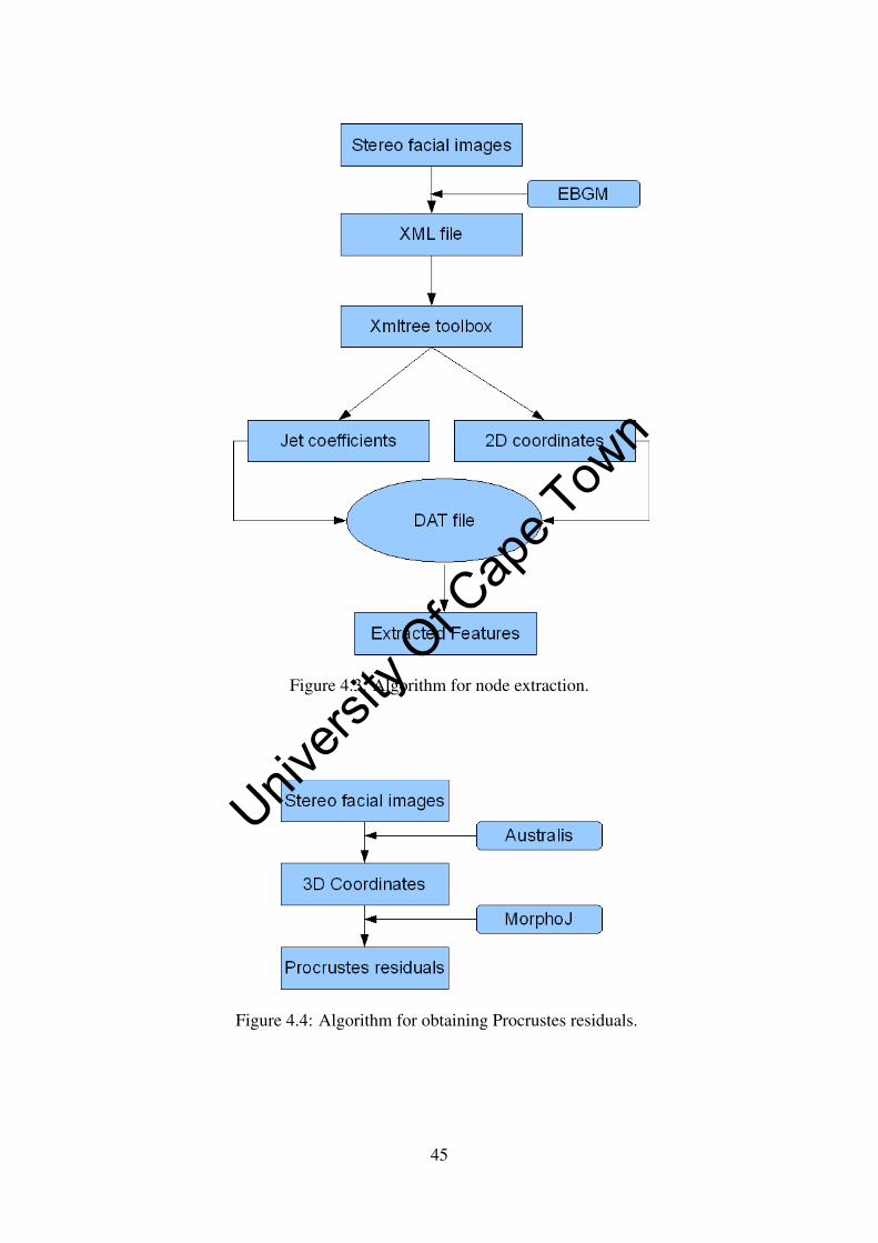
Figure 4.3: Algorithm for node extraction.
Figure 4.4: Algorithm for obtaining Procrustes residuals.
45
Univers
ity O
f Cap
e Tow
n
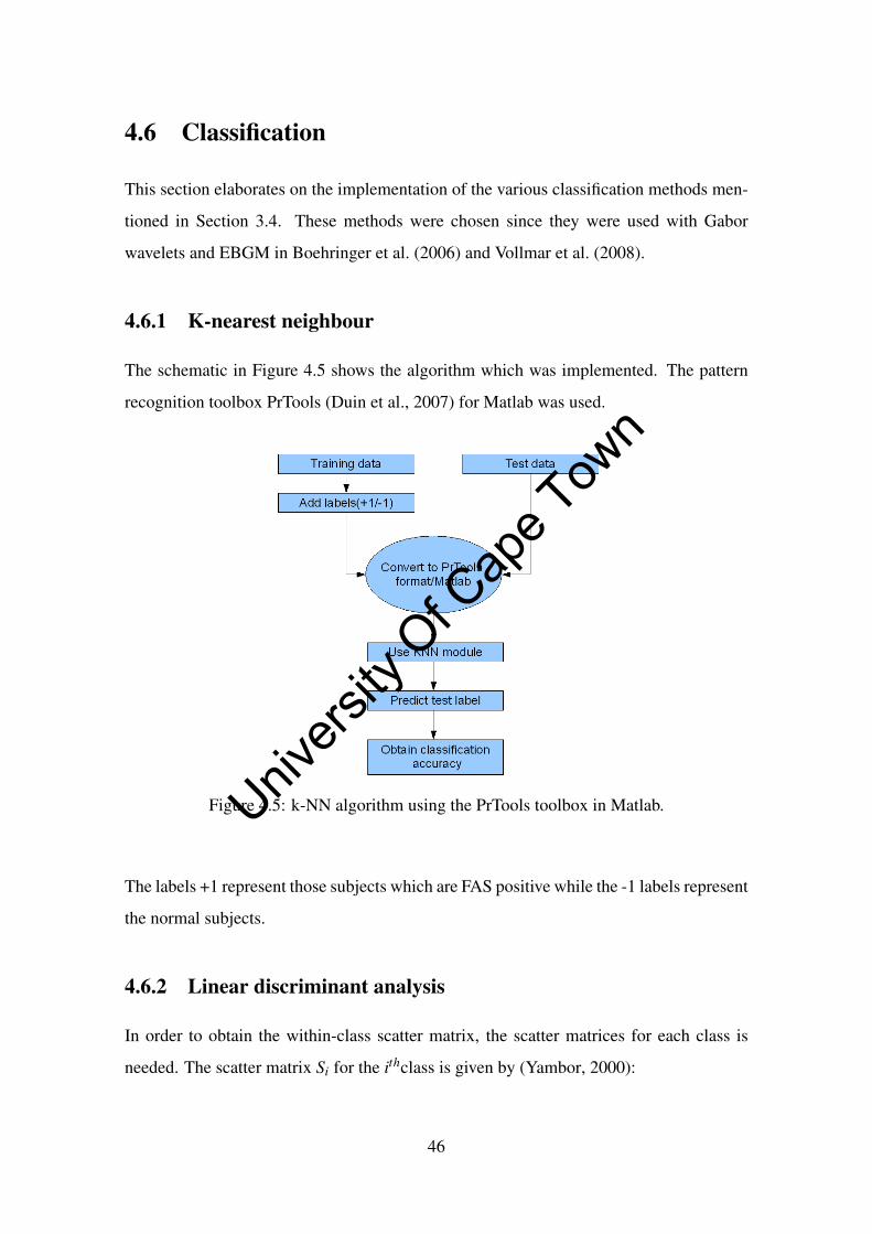
4.6 Classification
This section elaborates on the implementation of the various classification methods men-
tioned in Section 3.4. These methods were chosen since they were used with Gabor
wavelets and EBGM in Boehringer et al. (2006) and Vollmar et al. (2008).
4.6.1 K-nearest neighbour
The schematic in Figure 4.5 shows the algorithm which was implemented. The pattern
recognition toolbox PrTools (Duin et al., 2007) for Matlab was used.
Figure 4.5: k-NN algorithm using the PrTools toolbox in Matlab.
The labels +1 represent those subjects which are FAS positive while the -1 labels represent
the normal subjects.
4.6.2 Linear discriminant analysis
In order to obtain the within-class scatter matrix, the scatter matrices for each class is
needed. The scatter matrix Si for the ithclass is given by (Yambor, 2000):
46
Univers
ity O
f Cap
e Tow
n

Si = ∑x∈X
(x−mi)(x−mi)T
where mi is the mean of each class.
The within-class scatter matrix Sw is given by:
Sw =C
∑i=1
Si
where C is the number of classes. In our case, since there are only 2 classes (positive FAS
and normal), the within-class scatter matrix is the sum of the class scatter matrices S1 (for
class 1) and S2 (for class 2).
The between-class scatter matrix SB is given by:
SB =C
∑i=1
(mi−m)(mi−m)T
where m is the mean of all the classes. As with PCA, we solve for the eigenvectors and
eigenvalues of the equation:
SBV = hSwV
where V are the eigenvalues and h are the eigenvectors. The eigenvectors are sorted by
their associated eigenvalues from high to low and the first C−1 eigenvectors are retained.
4.6.3 Support vector machines
The linear kernel function was used for the SVM classifier. The general algorithm for
the classification process is shown in Figure 4.6. During classification, the classifiers
distinguish between given sets of binary labeled training data with a hyper-plane which
is maximally distant from them (‘maximum margin hyper-plane’). For cases that are not
linearly separable, ‘kernel methods’ can be used for a non linear mapping to a feature
47
Univers
ity O
f Cap
e Tow
n
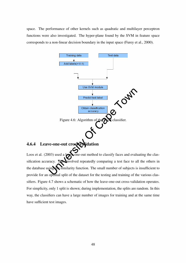
space. The performance of other kernels such as quadratic and multilayer perceptron
functions were also investigated. The hyper-plane found by the SVM in feature space
corresponds to a non-linear decision boundary in the input space (Furey et al., 2000).
Figure 4.6: Algorithm of the SVM classifier.
4.6.4 Leave-one-out cross-validation
Loos et al. (2003) used a leave-one-out method to classify faces and evaluating the clas-
sification accuracy. This involved repeatedly comparing a test face to all the others in
the database using the similarity function. The small number of subjects is insufficient to
provide for an optimal split of the dataset for the testing and training of the various clas-
sifiers. Figure 4.7 shows a schematic of how the leave-one-out cross-validation operates.
For simplicity, only 1 split is shown; during implementation, the splits are random. In this
way, the classifiers can have a large number of images for training and at the same time
have sufficient test images.
48
Univers
ity O
f Cap
e Tow
n

Figure 4.7: Schematic of leave-one-out cross-validation.
4.7 Principal component analysis
4.7.1 Snapshot PCA
The method of eigenvector selection described in Section 3.4.4 works very well on datasets
with a relatively small number of features. However, in our case, the number of features
is 1260 or more as will be seen later. This would give us a covariance matrix of size
(1260 x 1260) or more. Problems arise when attempting to evaluate the eigenvectors and
the eigenvalues of such a large matrix. It was therefore decided to use a method called
the ‘snapshot PCA’, (described below) which reduces computing time considerably but
achieves the same result as the method described in Section 3.4.4.
When analyzing a matrix X of size NxM (where N is the number of rows and M is the
number of columns), the maximum number of non-zero eigenvectors is min (N−1,M−1).
The eigenvalues of XXT are the same as those of XT X and the eigenvectors of XXT are the
same as those of XT X multiplied by X normalised. This is known as the snapshot method
for PCA. The following steps show the method in detail (Yambor, 2000):
xi =[xi
1 . . . xiN]T
49
Univers
ity O
f Cap
e Tow
n

xi =[xi−m
], where m =
1P
P
∑i=1
xi
X =[x1 x2 . . . xP]
These three steps are the same in the original PCA method, that is, subtracting the total
mean m from each subject xi and grouping them to form the data matrix.
The covariance matrix is then calculated by:
Ω′ = XT X
The eigenvectors and eigenvalues are found by:
Ω′V ′ = h′V ′
where
V ′ = eigenvectors,
h′= eigenvalues
The eigenvectors vi of XXT are found by:
V = XV ′
and
vi =vi
‖ vi ‖
The first of the above 2 steps consists of multiplying the eigenvectors of Ω′ by X and the
second step divides the individual eigenvectors by their norm.
50
Univers
ity O
f Cap
e Tow
n

The eigenvectors are then ordered as before, by selecting the eigenvectors corresponding
to the highest eigenvalues. These are used as the new axes of the dataset.
4.7.2 Principal component selection
As mentioned in Section 3.4.4, PCA aims to reduce the dimensionality of the data for
more accurate classification and also to obtain faster results by reducing the computational
time. The selection of the principal components (PCs) plays an important role in this
process. In this section we investigate a few PC selection schemes and also compare their
effect on the classification accuracy. The various methods are described below (Yambor,
2000):
1. Selecting the PCs corresponding to non-zero eigenvalues.
2. Eliminating the last 40% of the ordered PCs.
3. Calculating the ‘energy’ of the ith eigenvector by the following formula (this is
known as the ‘energy dimension’ method) :
ei =
∑iλ j
j=1
∑kλ j
j=i
where ei is the energy of the ith eigenvector , ∑iλ j
j=1is the sum of the first i (sorted) eigenval-
ues and ∑kλ j
f =iis the sum of the all the eigenvalues. The number of PCs selected depends
on whether ei is greater than a threshold. A typical value of the threshold is 0.9.
4.8 Varying graph structure
As mentioned in Section 4.1, the landmarks chosen to define the graph structure are those
which are important in discriminating between FAS and normal subjects, according to the
literature. Therefore, we perform experiments investigating the classification accuracy
when using different graph structures. In the first experiment, a grid using 30 manually
51
Univers
ity O
f Cap
e Tow
n

placed landmarks was used and the classification results were compared to the results of
using 30 automatically placed landmarks as well as 48 automatically placed landmarks.
The 30-landmark graph represents those facial features deemed important in FAS diag-
nosis (see Figure 4.1). The 48 node graph was used in (Loos et al., 2003; Vollmar et al.,
2008).
The term ‘manual’ indicates that the initial landmark location was done automatically but
was then corrected manually by moving the nodes to the desired location. This was aided
by the ‘magnifier’ function in the EBGM software which increased the accuracy of the
overall landmark location.
The various graphs used are shown in the Figures 4.8, 4.9, and 4.10.
Figure 4.8: Manually labeled graph of 30 nodes detected on an image.
52
Univers
ity O
f Cap
e Tow
n

Figure 4.9: Automatically labeled graph of 30 nodes detected on an image.
Figure 4.10: Automatically detected graph of 48 nodes.
4.9 Analysing the datasets
All the extracted features from EBGM and Procrustes analysis were stored in a format
which were compatible with Matlab. Statistical calculations in this section were all per-
formed using Matlab.
53
Univers
ity O
f Cap
e Tow
n

4.9.1 Dataset 1
The database consisted of a 5-year-old group and a 12-year-old group. The experiments
were performed separately on the two groups and on a larger combined group. The pur-
pose of the experiments was to investigate the performance of the classifiers and to com-
pare the outcome of the different graphs used. The groups were also investigated indi-
vidually in order to verify the effect of age on the classification accuracy, sensitivity and
specificity. As mentioned earlier, leave-one-out cross-validation was used to obtain the
classification accuracy. Sensitivity is defined as the proportion of true positives correctly
identified as positive while specificity is the proportion of true negatives correctly identi-
fied as negative. The classification accuracy for different principal component selection
schemes was examined.
4.9.2 Dataset 2
This group was made of up subjects of a similar age (Section 4.2). Only the methods
which proved to be successful with dataset 1 were investigated with this group. As with
dataset 1, the classification accuracies, sensitivities and specificities are obtained using
leave-one-out cross-validation.
54
Univers
ity O
f Cap
e Tow
n
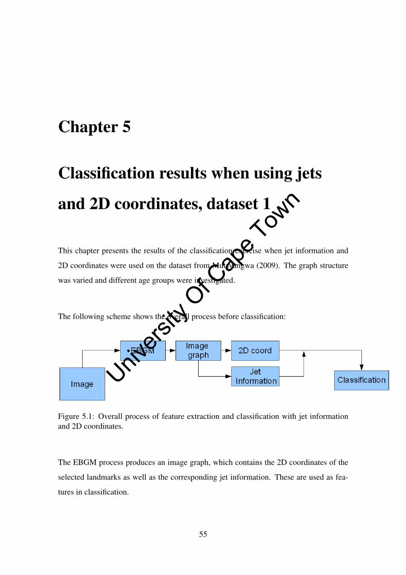
Chapter 5
Classification results when using jets
and 2D coordinates, dataset 1
This chapter presents the results of the classification exercise when jet information and
2D coordinates were used on the dataset from Mutsvangwa (2009). The graph structure
was varied and different age groups were investigated.
The following scheme shows the overall process before classification:
Figure 5.1: Overall process of feature extraction and classification with jet informationand 2D coordinates.
The EBGM process produces an image graph, which contains the 2D coordinates of the
selected landmarks as well as the corresponding jet information. These are used as fea-
tures in classification.
55
Univers
ity O
f Cap
e Tow
n

5.1 Classification of combined age groups using jets and
2D coordinates
Table 5.1 shows the the classification accuracies when using kNN and LDA on the com-
bined age group using the graph with 30 manually placed nodes.
Table 5.1: Classification results when the 30-node manual graph was used.
Table 5.2 shows the classification accuracies when using kNN and LDA classifiers on the
combined age group using the graph with 30 automatically placed nodes.
56
Univers
ity O
f Cap
e Tow
n

Table 5.2: Classification results when the 30-node automatic graph was used.
Table 5.3 shows the classification accuracies when using kNN and LDA classifiers on the
combined age group using the graph with 48 automatically placed nodes.
Table 5.3: Classification results when the 48-node automatic graph was used.
57
Univers
ity O
f Cap
e Tow
n
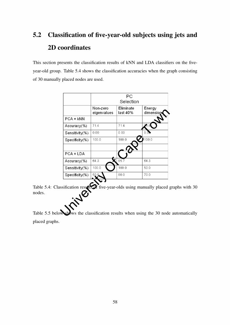
5.2 Classification of five-year-old subjects using jets and
2D coordinates
This section presents the classification results of kNN and LDA classifiers on the five-
year-old group. Table 5.4 shows the classification accuracies when the graph consisting
of 30 manually placed nodes are used.
Table 5.4: Classification results of five-year-olds using manually placed graphs with 30nodes.
Table 5.5 below shows the classification results when using the 30 node automatically
placed graphs.
58
Univers
ity O
f Cap
e Tow
n
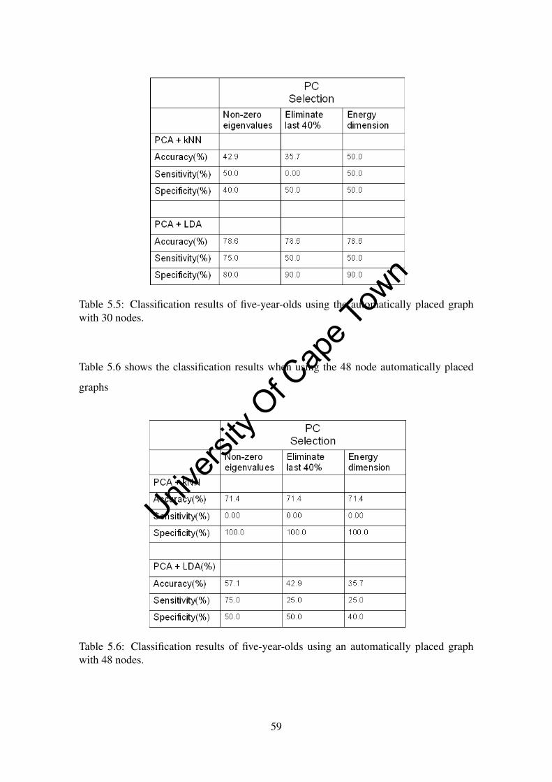
Table 5.5: Classification results of five-year-olds using the automatically placed graphwith 30 nodes.
Table 5.6 shows the classification results when using the 48 node automatically placed
graphs
Table 5.6: Classification results of five-year-olds using an automatically placed graphwith 48 nodes.
59
Univers
ity O
f Cap
e Tow
n

5.3 Classification of twelve-year-old subjects using jets
and 2D coordinates
This section presents the results of classification on the twelve-year-old subjects.
Table 5.7 below shows the results of classification when the 30-node manual graph was
used.
Table 5.7: Classification results of twelve-year-olds using the manually placed graph with30 nodes.
Table 5.8 shows the results of the classification when the 30-node automatically placed
graph was used.
60
Univers
ity O
f Cap
e Tow
n
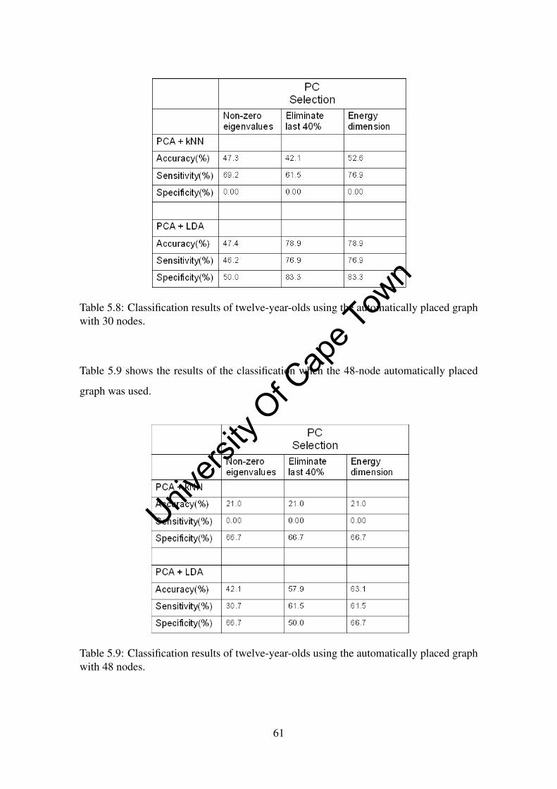
Table 5.8: Classification results of twelve-year-olds using the automatically placed graphwith 30 nodes.
Table 5.9 shows the results of the classification when the 48-node automatically placed
graph was used.
Table 5.9: Classification results of twelve-year-olds using the automatically placed graphwith 48 nodes.
61
Univers
ity O
f Cap
e Tow
n

5.4 Support vector machine classification using jets and
2D coordinates
The experiments using the SVM classifier were performed separately since no PCA was
needed before classification. The different parameters for the SVM classifier were the
linear kernel, quadratic kernel and the multilayer perceptron.
Table 5.10 shows the classification results when the linear kernel was used.
Table 5.10: Results of the SVM classifier with linear kernel.
Table 5.11 shows the classification results when the quadratic kernel was used.
62
Univers
ity O
f Cap
e Tow
n
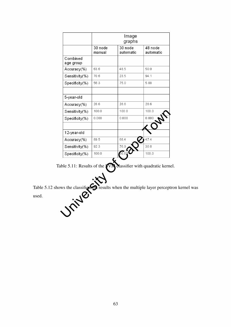
Table 5.11: Results of the SVM classifier with quadratic kernel.
Table 5.12 shows the classification results when the multiple layer perceptron kernel was
used.
63
Univers
ity O
f Cap
e Tow
n
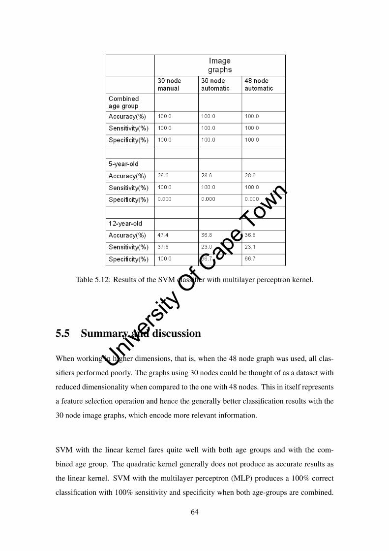
Table 5.12: Results of the SVM classifier with multilayer perceptron kernel.
5.5 Summary and discussion
When working in higher dimensions, that is, when the 48 node graph was used, all clas-
sifiers performed poorly. The graphs using 30 nodes could be thought of as a dataset with
reduced dimensionality when compared to the one with 48 nodes. This in itself represents
a feature selection operation and hence the generally better classification results with the
30 node image graphs, which encode more relevant information.
SVM with the linear kernel fares quite well with both age groups and with the com-
bined age group. The quadratic kernel generally does not produce as accurate results as
the linear kernel. SVM with the multilayer perceptron (MLP) produces a 100% correct
classification with 100% sensitivity and specificity when both age-groups are combined.
64
Univers
ity O
f Cap
e Tow
n
However, when the age-groups are analysed separately, MLP performs poorly. These
observations show that there is a high degree of variability with the quadratic and MLP
classification accuracies. The differences in the classification accuracies may be a result
of the nature of those classifiers and do not represent the true separability of the dataset.
There were 15 five-year-old subjects of which 11 were normal and 4 were FAS positive.
This small number of FAS positive subjects in this age group led to low sensitivities and
higher specificities. The twelve-year-old group consisted of 13 FAS positive subjects and
6 normal subjects. The sensitivities in this age group were higher while the specificities
were usually lower with kNN. The generally low kNN classification accuracies may be
explained by the relatively large number of features compared to the number of subjects.
Boehringer et al. (2006) and Vollmar et al. (2008) observed that manual placement of
nodes results in better classification accuracies. Automatic landmark location can result in
the nodes being placed at incorrectly placed landmarks. The data point thus encodes noise
instead of useful information, leading to lower classification accuracies. No such trend
was observed in the present study for 30 node graphs across all age groups. However, the
results for the combined age group appear to be most reliable, given the more balanced
combination of FAS and non-FAS subjects in this group. For this group, LDA produced
better results on the 30-node manual graph. Considering the superiority of LDA and its
improved performance on the 30-node manual graph, for the combined age group, the
30-node manual graph is used in the chapters that follow.
Table 5.13 shows the best set of results for the different classifiers, with the 30-node-
manual graphs. LDA is the classifier which performs most consistently while the PC
selection using the energy dimension also performs well. SVM can only be used consis-
tently with the linear kernel.
65
Univers
ity O
f Cap
e Tow
n
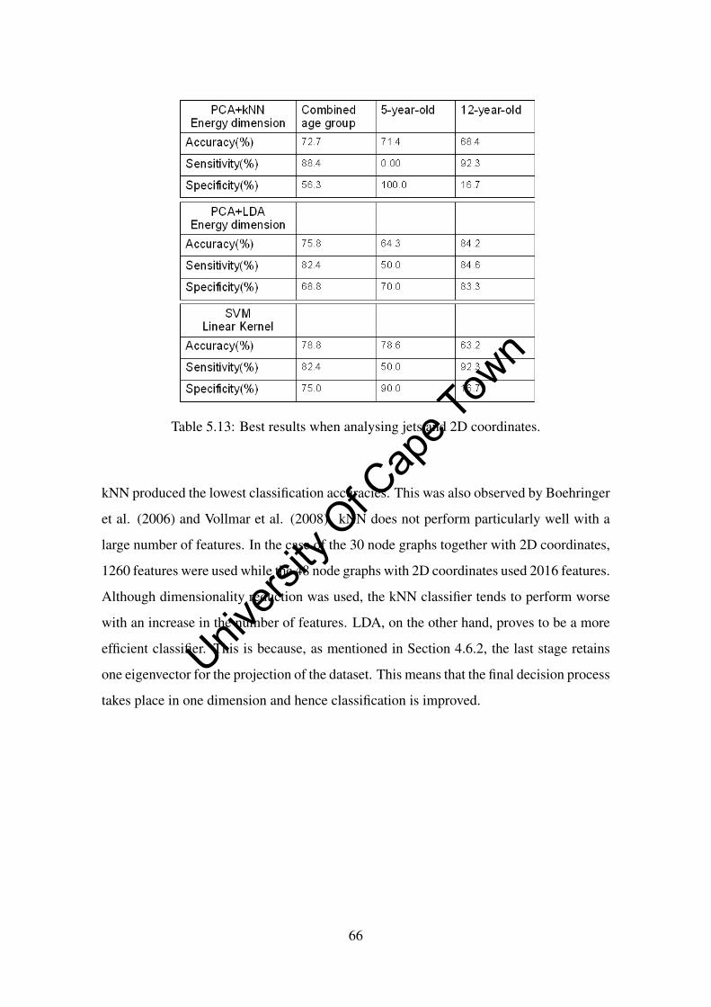
Table 5.13: Best results when analysing jets and 2D coordinates.
kNN produced the lowest classification accuracies. This was also observed by Boehringer
et al. (2006) and Vollmar et al. (2008). kNN does not perform particularly well with a
large number of features. In the case of the 30 node graphs together with 2D coordinates,
1260 features were used while the 48 node graphs with 2D coordinates used 2016 features.
Although dimensionality reduction was used, the kNN classifier tends to perform worse
with an increase in the number of features. LDA, on the other hand, proves to be a more
efficient classifier. This is because, as mentioned in Section 4.6.2, the last stage retains
one eigenvector for the projection of the dataset. This means that the final decision process
takes place in one dimension and hence classification is improved.
66
Univers
ity O
f Cap
e Tow
n

Chapter 6
Classification results when using jets
and Procrustes residuals, dataset 1
The results shown here are based on the classification of jet information and Procrustes
residuals, which are representative of the 3D coordinates of the facial landmarks. Pro-
crustes residuals were used instead of 3D coordinates since Vollmar et al. (2008) stan-
dardised the 2D coordinates in their application of the same methods and Procrustes anal-
ysis is a form of standardisation, by requiring all shapes to be compared to the centroid
of the group. This dataset is the same as that used in Mutsvangwa (2009) and was also
used in Chapter 5. The use of Procrustes residuals rather than 3D coordinates facilitates
comparison with the results of Mutsvangwa (2009). Since labeling of the stereo facial
images before the application of generalised Procrustes analysis was done manually, only
the jet information from the manually labeled graph with 30 nodes was used.
The scheme in Figure 6.1 shows how the Procrustes residuals and the jet information were
used for classification.
67
Univers
ity O
f Cap
e Tow
n

Figure 6.1: Overall process of including 3D information with jet information for classifi-cation.
The EBGM process produces, as before, 2D coordinates of specific landmarks together
with the corresponding jet information. The 3D coordinates and Procrustes residuals are
obtained from the bundle adjustment and Procrustes superimposition processes, respec-
tively. Stereo facial images were used for this purpose. However, in this case, only the
Procrustes residuals and jet information were used as features in classification.
6.1 Classification of combined age groups using jets and
Procrustes residuals
Table 6.1 shows the classification results when 3D information, that is, the Procrustes
residuals, are included in the dataset.
68
Univers
ity O
f Cap
e Tow
n
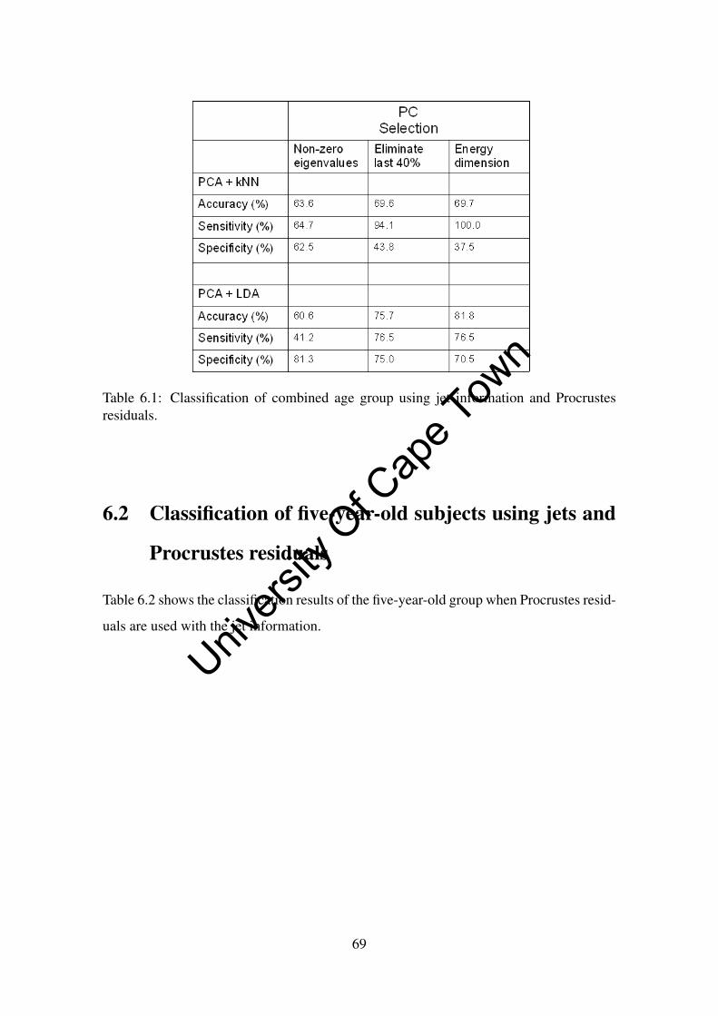
Table 6.1: Classification of combined age group using jet information and Procrustesresiduals.
6.2 Classification of five-year-old subjects using jets and
Procrustes residuals
Table 6.2 shows the classification results of the five-year-old group when Procrustes resid-
uals are used with the jet information.
69
Univers
ity O
f Cap
e Tow
n

Table 6.2: Classification of five-year-old subjects using jet information and Procrustesresiduals.
6.3 Classification of twelve-year-old subjects using jets
and Procrustes residuals
Table 6.3 show the results of the classification on the twelve-year-old group of subjects.
70
Univers
ity O
f Cap
e Tow
n

Table 6.3: Classification of twelve-year-old subjects using jet information and Procrustesresiduals.
6.4 Support vector machine classification using jets and
Procrustes residuals
Table 6.4 shows the results of the classification using SVM on all age groups and when
the linear kernel is used. The quadratic and multilayer perceptron kernels were not used,
given their poor performance in Chapter 5.
71
Univers
ity O
f Cap
e Tow
n
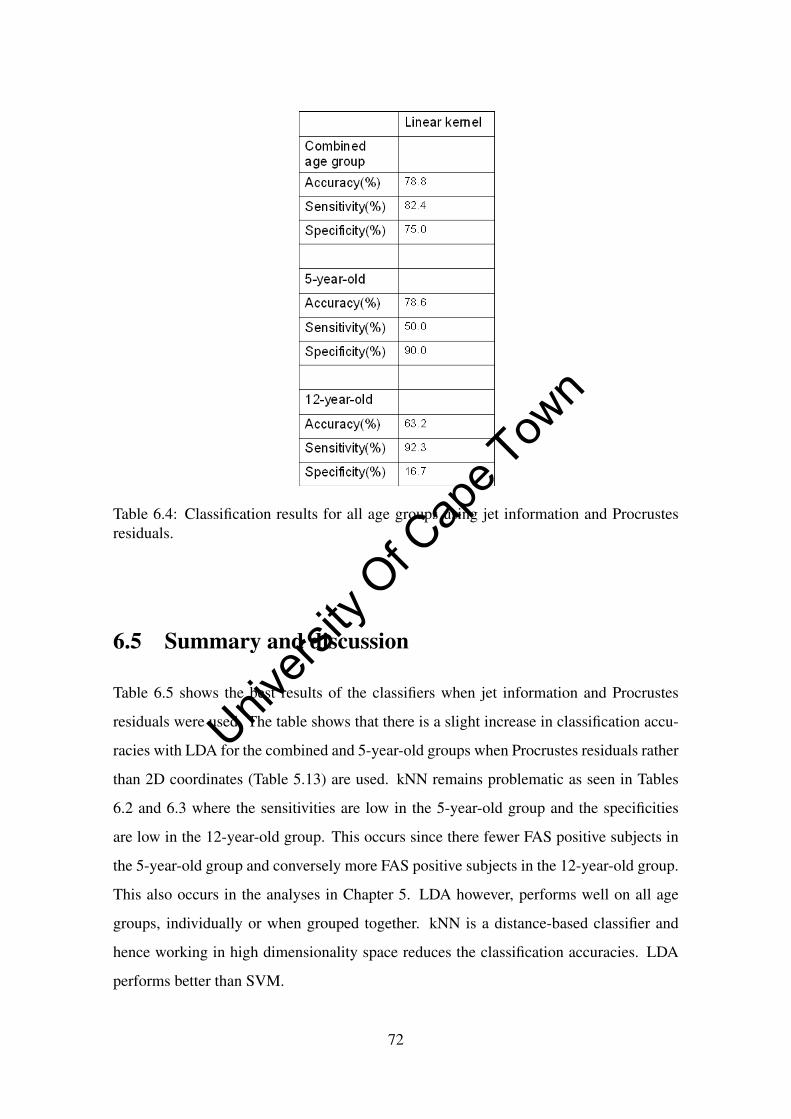
Table 6.4: Classification results for all age groups using jet information and Procrustesresiduals.
6.5 Summary and discussion
Table 6.5 shows the best results of the classifiers when jet information and Procrustes
residuals were used. The table shows that there is a slight increase in classification accu-
racies with LDA for the combined and 5-year-old groups when Procrustes residuals rather
than 2D coordinates (Table 5.13) are used. kNN remains problematic as seen in Tables
6.2 and 6.3 where the sensitivities are low in the 5-year-old group and the specificities
are low in the 12-year-old group. This occurs since there fewer FAS positive subjects in
the 5-year-old group and conversely more FAS positive subjects in the 12-year-old group.
This also occurs in the analyses in Chapter 5. LDA however, performs well on all age
groups, individually or when grouped together. kNN is a distance-based classifier and
hence working in high dimensionality space reduces the classification accuracies. LDA
performs better than SVM.
72
Univers
ity O
f Cap
e Tow
n
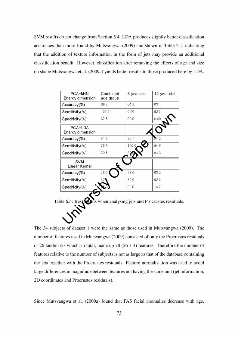
SVM results do not change from Section 5.4. LDA produces slightly better classification
accuracies than those found by Mutsvangwa (2009) and shown in Table 2.1, indicating
that the addition of texture information in the form of jets may provide an additional
classification benefit. However, classification after removing the effects of age and size
on shape Mutsvangwa et al. (2009a) yields better results to those produced here by LDA.
Table 6.5: Best results when analysing jets and Procrustes residuals.
The 34 subjects of dataset 1 were the same as those used in Mutsvangwa (2009). The
number of features used in Mutsvangwa (2009) consisted of only the Procrustes residuals
of 26 landmarks which, in total, made up 78 (26 x 3) features. Therefore the number of
features relative to the number of subjects is not as large as that of the database containing
the jets together with the Procrustes residuals. Feature normalisation was used to avoid
large differences in magnitude between features not having the same unit (jet information,
2D coordinates and Procrustes residuals).
Since Mutsvangwa et al. (2009a) found that FAS facial anomalies decrease with age,
73
Univers
ity O
f Cap
e Tow
n

lower classification accuracy is expected in 12-year-olds. While the LDA sensitivity is
higher in 5-year-olds, overall accuracy is similar in the 5 and the 12-year-old groups.
Larger sample size maybe be needed for definitive conclusions in the absence of adjust-
ment for the effects of size and age on shape, as made by Mutsvangwa et al. (2009a).
74
Univers
ity O
f Cap
e Tow
n

Chapter 7
Classification results with jets and
Procrustes residuals, dataset 2
This chapter shows the results of analysing the dataset of 7-year old subjects acquired
during the study and described in Section 4.2.2.
7.1 Classification with PCA and LDA
Because the addition of 3D information produced slightly better results with LDA in
Chapter 6, only jets in combination with Procrustes residuals were analysed. Manual
landmark location and a 30-node graph was used for EBGM.
Table 7.1 shows the classification results when using PCA and LDA on the second dataset.
kNN classification was not performed, given its poor performance in Chapter 6.
75
Univers
ity O
f Cap
e Tow
n
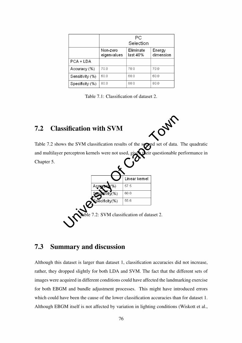
Table 7.1: Classification of dataset 2.
7.2 Classification with SVM
Table 7.2 shows the SVM classification results of the second set of data. The quadratic
and multilayer perceptron kernels were not used, given their questionable performance in
Chapter 5.
Table 7.2: SVM classification of dataset 2.
7.3 Summary and discussion
Although this dataset is larger than dataset 1, classification accuracies did not increase,
rather, they dropped slightly for both LDA and SVM. The fact that the different sets of
images were acquired in different conditions could have affected the landmarking exercise
for both EBGM and bundle adjustment processes. This might have introduced errors
which could have been the cause of the lower classification accuracies than for dataset 1.
Although EBGM itself is not affected by variation in lighting conditions (Wiskott et al.,
76
Univers
ity O
f Cap
e Tow
n
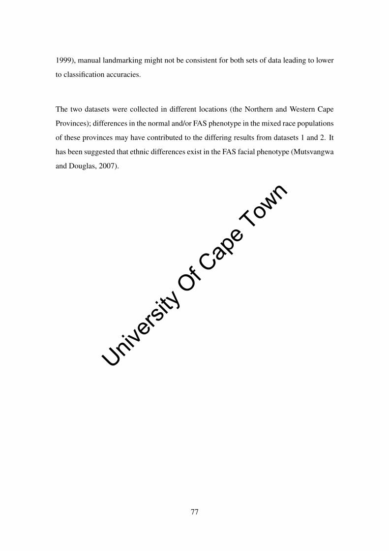
1999), manual landmarking might not be consistent for both sets of data leading to lower
to classification accuracies.
The two datasets were collected in different locations (the Northern and Western Cape
Provinces); differences in the normal and/or FAS phenotype in the mixed race populations
of these provinces may have contributed to the differing results from datasets 1 and 2. It
has been suggested that ethnic differences exist in the FAS facial phenotype (Mutsvangwa
and Douglas, 2007).
77
Univers
ity O
f Cap
e Tow
n

Chapter 8
Conclusions and recommendations
The study made use of Gabor wavelets and elastic bunch graph matching, an already
successful approach in discriminating between various facial malformation syndromes
(Loos et al., 2003; Boehringer et al., 2006; Vollmar et al., 2008), to distinguish between
FAS and normal subjects. In addition to the jet information obtained from EBGM, 3D
information was incorporated in the dataset to analyse whether shape information would
increase the classification accuracy.
The results indicate that jet information together with 2D information give classifica-
tion accuracies that vary, depending on the classifier used, the type of image graph used
(manual or automatic) and the number of nodes used (30 or 48). No clear trend was
observed with respect to manual compared to automatic labelling and classification ac-
curacy. However, manual landmarking resulted in improved classification with the best
performing classifier and the most balanced age group. A reliable automatic landmark
location algorithm would reduce the time spent on manual labelling of landmarks
The results show that the classification accuracies vary widely from one classifier to an-
other. LDA performed most consistently. SVM using the linear kernel also showed some
promising results on the first dataset.
78
Univers
ity O
f Cap
e Tow
n

In Chapter 6, 2D coordinates were replaced by 3D information in the form of Procrustes
residuals. The results indicate a slight increase in the classification accuracies in dataset
1 when using LDA. The increase in accuracy may be attributed to the additional spatial
shape information included in the experiments. This shape information is very important
for differentiating FAS subjects from normal subjects as a result of the mid-face hypopla-
sia (contraction of the mid-face), which can only be observed in the facial profile.
The 30-node graphs gave better accuracies than the 48-node graphs. The 30 nodes, which
were mostly located in the midface area, contained the more discriminating features be-
tween FAS and normal. However, the number of features in the dataset was still quite
large when compared to the number of subjects. Principal component analysis reduced
the dimensionality. One could attempt to investigate feature selection schemes like a pop-
ulation based incremental learning scheme (PBIL) or a genetic algorithm (GA).
The larger dataset analysed in Chapter 7 produced lower classification accuracies possibly
due to different imaging conditions and/or dataset composition.
Removing the effects of age and size on shape by regression, as done by Mutsvangwa
et al. (2009a) may improve classification accuracies.
79
Univers
ity O
f Cap
e Tow
n

Bibliography
Adams, D., Rohlf, F., Slice, D., 2004. Geometric morphometrics ten years of progress
following the revolution. Ital J Zool 71, 5–16.
Astley, S., 2006. Comparison of the 4-digit diagnostic code and the hoyme diagnostic
guidelines for fetal alcohol spectrum disorders. Pediatrics: An official journal of the
american acedemy of pediatrics 118, 1532–1545.
Astley, S., Clarren, S., 1995. A fetal alcohol syndrome screening tool. Alcohol Clin Exp
Res 6, 1565–1571.
Astley, S., Clarren, S., 1996. A case definition and photographic screening tool for the
facial phenotype of fetal alcohol syndrome. J Pediatr 129, 33–41.
Astley, S., Clarren, S., 2000. Diagnosing the full spectrum of fetal alcohol exposed indi-
viduals: introducing the 4-digit diagnostic code. Alcohol Alcohol 35, 400–410.
Balakrishnama, S., Ganapathiraju, A., 1998. Linear discriminant analysis - a brief tutorial.
Tech. rep., Institute for Signal and Information Processing Department of Electrical and
Computer Engineering Mississippi State University.
Boehringer, S., Vollmar, T., Tasse, C., Wurtz, R., Gillensen-Kaesbach, G., Horsthemke,
B., Wieczorek, D., 2006. Syndrome identification based on 2d analysis software. Euro-
pean Journal of Human Genetics, 1–8.
Bolme, D., 2003. Elastic bunch graph matching. Master’s thesis, Colorado State Univer-
sity.
Burd, L., Cotsonas, T., Martsolf, J., Kerbeshian, J., 2003. Recognition and management
of fetal alcohol syndrome. Neurotoxicology and Teratology 25, 681–688.
80
Univers
ity O
f Cap
e Tow
n
Burges, C., 1998. A tutorial on support vector machines for pattern recognition. Data
Mining and Knowledge Discovery 2, 121–167.
Cawley, G., Talbot, N., 2003. Effcient leave one out cross-validation of kernel fisher dis-
criminant classifiers. The Journal of the Pattern Recognition Society 36, 2585–2592.
Christianini, N., Shawe-Taylor, J., 2000. An introduction to support vector machines and
other kernel-based learning methods. The press syndicate of the University of Cam-
bridge.
Clarren, S., Sampson, P., Larsen, J., 1987. Facial effects of fetal alcohol exposure: assess-
ment by photographs and morphometric analysis. Am J Med Genet 26, 651–666.
Dai, D., Yan, H., 2007. Wavelets and Face Recognition.
Dalal, A., Phadke, S., 2007. Morphometric analysis of face in dysmorphology. Computer
methods and programs in biomedicine 85, 165–172.
Douglas, T., 2004. Image processing for craniofacial landmark identification and mea-
surement: a review of photogrammetry and cephalometry. Computerized Medical
Imaging and Graphics 28, 401–409.
Douglas, T., Martinez, F., Meintjes, E., Vaughan, C., Viljoen, D., 2003. Eye feature ex-
traction for diagnosing the facial phenotype associated with fetal alcohol syndrome.
Med. Biol. Eng. Computer 41, 101–106.
Dryden, I., Mardia, K., 1998. Statistical Shape Analysis. John Wiley & Sons.
DTREG, 2003. Software for predictive modelling and forecasting. Web.
URL http://www.dtreg.com/lda.htm
Duin, R., Juszczak, P., Paclik, P., Pekalska, E., de Ridder, D., Tax, D., Verzakov, S.,
2007. Prtools version 4.1: A matlab toolbox for pattern recognition. Delft University
of Technology.
Fang, S., McLaughlin, J., Fang, J., Autti-Ramo, I., Fagerlund, A., Jacobson, S., Robinson,
L., Hoyme, H., Mattson, S., Riley, E., Zhou, F., Ward, R., Moore, E., Foroud, T., 2008.
81
Univers
ity O
f Cap
e Tow
n
Automated diagnosis of fetal alcohol syndrome using 3d facial image analysis. Orthod
Craniofac Res 11, 162–171.
Farkas, L., 1998. Anthropometry of the head and face. New York: Raven Press.
Ferrario, V., Sforza, C., Schmitz, J., MianiJr, A., Taronu, G., 1995. Fourier analysis of
human soft tissue facial shape: sex differences in normal adults. J Anat 187, 593–602.
Furey, T., Cristianini, N., Duffy, N., Bednarski, D., Schummer, M., D.Haussler, 2000.
Support vector machine classification and validation of cancer tissue samples using
microarray expression data. Bioinformatics 16, 906–914.
Grobbelaar, R., Douglas, T., 2007. Stereo image matching for facial feature measurement
to aid in fetal alcohol syndrome screening. Medical Engineering & Physics 29, 459–
464.
Halazonetis, D., 2004. Morphometrics for cephalometric diagnosis. Am J Orthod Dento-
facial Orthop 125, 571–81.
Hammond, P., 2007. The use of 3d face shape modelling in dysmorphology. Arch. Dis.
Child 92, 1120–1126.
Hammond, P., Hutton, T., Allanson, J., Campbell, L., Hennekam, R., Holden, S., Murphy,
K., Pattan, M. A., Shaw, A., Temple, I., Trotter, M., Winter, R., 2004. 3d analysis of
facial morphology. American Journal of medical genetics 126A, 339–348.
Henessy, R., Baldwin, P., Browne, D., Kinsella, A., Waddington, J., 2007. Three-
dimensional laser surface imaging and geometric morphometrics resolve frontonasal
dysmorphology in schizophrenia. Biol Psychiatry 61, 1187–1194.
Holden, E., Owens, R., 2002. Automatic facial point detection. In: The 5th Asian Confer-
ence on Computer Vision.
Hoyme, H. E., , May, P. A., , Kalberg, W. O., Kodituwakku, P., Gossage, J. P., M.Trujillo,
P., Buckley, D. G., Miller, J. H., Aragon, A. S., Khaole, N., Viljoen, D. L., Jones,
K. L., Robinson., L. K., 2005. A practical clinical approach to diagnosis of fetal alcohol
82
Univers
ity O
f Cap
e Tow
n

spectrum disorders: Clarification of the 1996 institute of medicine criteria. Pediatrics:
An official journal of the american acedemy of pediatrics 115, 39–47.
Huang, J., Jain, A., Fang, S., Riley, E., 2005. Using facial images to diagnose fetal alcohol
syndrome (fas). Proc. of International Conference on Information Technology: Coding
and Computing 1, 66–71.
Janecek, A., Gansterer, W., 2008. On the relationship between feature selection and clas-
sification accuracy. In: JMLR: Workshop and Conference Proceedings. Vol. 4. pp. 90–
105.
Jones, K., Smith, D., 1973. Recognition of the fetal alcohol syndrome in early infancy.
Lancet 2, 999–1001.
Klecka, W., 1980. Discriminant Analysis. SAGE.
Klingenberg, C., 2008. Morphoj, faculty of life sciences, university of manchester.
Loos, H., Wieczorek, D., Wurtz, R., Malsburg, C., Horsthemke, B., 2003. Computer-
based recognition of dysmorphic faces. European Journal of Human Genetics 11, 555–
560.
May, P., Gossage, J., Marais, A., Adnams, C., Hoyme, H., Jones, K., Robinson, L.,
Khaole, N., Snell, C., Kalberg, W., Hendricks, L., Brooke, L., Stellavato, C., Viljoen,
D., 2007. The epidemiology of fetal alcohol syndrome and partial fas in a south african
community. Drug and Alcohol Dependence 88, 259–271.
McIntyre, G., Mossey, P., 2003. Size and shape measurement in contemporary cephalo-
metrics. Eur J Orthod 25, 231–242.
Meintjes, E., Douglas, T., Martinez, F., Vaughan, C., Adams, L., Stekhoven, A., Viljoen,
D., 2002. A stereo-photogrammetric method to measure the facial dysmorphology of
children in the diagnosis of fetal alcohol syndrome. Medical Engineering and Physics
28, 683–689.
83
Univers
ity O
f Cap
e Tow
n
Milborrow, S., Nicolls, F., 2007. Location facial features with an extended active shape
model. Master’s thesis, Department of Electrical Engineering, University of Cape
Town.
Mitchell, H., Newton, I., 2002. Medical photogrammetric measurement:overview and
prospects. ISPRS Journal of Photogrammetry & Remote Sensing 56, 286–294.
Moore, A., 2001. Support vector machines. School of Computer Science, Carnegie Mel-
lon University.
URL http://www.cs.cmu.edu/ awm/tutorials
Moore, E., Ward, R., Jamison, P., Morris, C., Bader, P., Hall, B., 2001. The subtle facial
signs of prenatal exposure to alcohol: an anthropometric approach. J Pediatr 139, 215–
9.
Moore, E., Ward, R., Wetherill, L., Rogers, J., Autti-Ra¨mo¨, I., Fagerlund, A., Jacobson,
S., Robinson, L., Hoyme, H., Mattson, S., Foroud, T., CIFASD, 2007. Unique facial
features distinguish fetal alcohol syndrome patients and controls in diverse ethnic pop-
ulations. Alcoholism: Clinical and Experimental Research 31, 1707–1713.
Mutsvangwa, T., 2009. Characterisation of the facial phenotype associated with fetal alco-
hol syndrome using stereo-photogrammetry and geometric morphometrics. Ph.D. the-
sis, University of Cape Town.
Mutsvangwa, T., Douglas, T., 2007. Morphometric analysis of facial landmark data to
characterize the facial phenotype associated with fetal alcohol syndrome. Journal of
Anatomy 210, 209–220.
Mutsvangwa, T., Meintjes, E., Viljoen, D., Douglas, T., 2009a. Morphometric analysis
and classification of the facial phenotype associated with fetal alcohol syndrome in 5-
and 12-year-old children. American Journal of Medical Genetics 152A (1), 32–41.
Mutsvangwa, T. E., Smit, J., Hoyme, H. E., Kalberg, W., Viljoen, D. L., Meintjes, E. M.,
Douglas, T. S., 2009b. Design, construction and testing of a stereophotogrammetric tool
for the diagnosis of fetal alcohol syndrome in infants. IEEE Transactions on Medical
Imaging 28(9), 1448–58.
84
Univers
ity O
f Cap
e Tow
n
Naftel, A., Trenouth, M., 2004. Stereo-assisted landmark detection for the analysis of
changes in 3-d facial shape. Informatics for health and social care 29, 137–155.
Norman McLeod, P. L. F., 2002. Morphology, Shape and Phylogeny. Taylor & Francis.
Parry, C., 2002. Alcohol problems in developing countries: Challenges for the new mil-
lennium. Suchtmed 2(4), 216–220.
Robinson, D., Blackwell, P., Stillman, E., Brook, A., 2001. Planar procrustes analysis of
tooth shape. Archives of Oral Biology 46, 191–199.
Rohlf, F., Slice, D., 1990. Extensions of the procrustes method for the optimal superim-
position of landmarks. Syst Zool 39, 40–59.
Shen, L., Bai, L., 2006. A review on gabor wavelets for face recognition. Pattern Anal
Applic 9, 273–292.
Slice, D., 2007. Geometric morphometrics. Annu. Rev. Anthropol. 36, 261–281.
Sokol, R., Chick, L., Martier, S., Salari, V., 1991. Morphometry of the neonatal fetal
alcohol syndrome face from ’snapshots’. Alcohol & Alcoholism, Suppl. 1, 531–534.
Song, Y., Huang, J., Zhou, D., Zha, H., Giles, C., 2007. Informative k-nearest neighbor
pattern classification. PKDD 4702, 248–264.
Souza, A., Ruiz, E., Cruz, A., 2000. Palpebral fissure morphology segmentation and mea-
surement using image processing-a semi automated method for detection eyelid related
pathologies. IEEE Engineering in medicine and biology 19, 114–119.
StatSoft, 1984-2008a. Web.
URL http://www.statsoft.com/textbook/stknn.html
StatSoft, 1984-2008b. Web.
URL http://www.statsoft.com/textbook/stsvm.html
Streissguth, A., Aase, J., Clarren, S., Randels, S., LaDue, R., Smith, D., 1991. Fetal
alcohol syndrome in adolescents and adults. JAMA 265, 1961–1967.
85
Univers
ity O
f Cap
e Tow
n

Viljoen, D., Gossage, J., Brooke, L., Adnams, C., Jones, K., Robinson, L., Hoyme, H.,
Snell, C., Khaole, N., Kodituwakku, P., Asante, K., Findlay, R., Quinton, B., Marais,
A., Kalberg, W., May, P., 2005. Fetal alcohol syndrome epidemiology in a south african
community: A second study of a very high prevalence area. J. Stud. Alcohol 66, 593–
604.
Vollmar, T., Maus, B., Wurtz, R., Gillensen-Kaesbach, G., Horsthemke, B., Wieczorek,
D., Boehringer, S., 2008. Impact of geometry on viewing angle on classification accu-
racy of 2d based analysis of dysmorphic faces. European Journal of Medical Genetics
51, 44–53.
Vukadinovic, D., Pantic, M., 2005. Fully automatic facial feature point detection using
gabor feature based boosted classifiers. In: IEEE International Conference on Systems,
Man and Cybernetics.
Wang, P., Barrett, F., Martin, E., Milanova, M., Gur, R., Gur, R., Kohler, C., Verma, R.,
2008. Automated video based facial expression analysis of neuropsychiatric disorders.
J Neurosci Methods 168(1), 224–238.
Wiskott, L., Fellous, J., Kruger, N., der Malsburg, C., 1999. Face recognition by elastic
bunch graph matching. CRC press.
Wong, J., A.K.Oh, E.Ohta, A.T.Hunt, G.F.Rogers, J.Mulliken, C.K.Deutsch, 2008. Valid-
ity and reliability of craniofacial anthropometric measurement of 3d digital photogram-
metric images. Cleft Palate-Craniofacial Journal 45 No 3.
Yambor, W., 2000. Analysis of pca-based and fisher discriminant-based image recogni-
tion. Tech. rep., Computer Science Department, Colorado State University.
86
Univers
ity O
f Cap
e Tow
n