Candidate number: 311990Word count: 6399

TP19: Spatial Networks and Human Mobility: An Application of the InterveningOpportunites Model to the London Cycle Hire Scheme

Supervisor: Dr. M. A. Porter

Human mobility drives a variety of physical phenomenon in the modern world. Our understandingof human mobility has been dominated by two theoretical models: the gravity model and the inter-vening opportunities (IO) model. In this thesis we derive these models with spatial network theoryformalism and consider their application to the London Cycle Hire Scheme (LCHS). We demon-strate theoretically why an opportunistic model is more appropriate than the Gravity model andshow that the most appropriate opportunistic model is an intervening opportunities model modifiedwith a theory of Spatial Dominance (IOSD) for the case of LCHS. Furthermore, we also challengethe convention of ignoring self-loops commonly employed when analysing physical networks, and weshow how self-loops found in the LCHS can be successfully assimilated into the application of theIOSD.

I. BACKGROUND

Although it is a difficult task, modelling human mo-bility is extremely important if we hope to understanda diverse range of physical systems from modelling viruspandemics [2] to traffic flows [3]. The difficulty stemsfrom the myriad of unknown factors associated with bothhuman-decision making and the physical systems them-selves. However, it has been shown that strong spatialand temporal patterns can exist [1] - in human mobilityand models have been developed that successfully de-scribe a variety of networks.

The understanding of human mobility is limited by theability to collect data about individuals. Given the in-creasingly sophisticated ability to track individuals, mod-elling human mobility has seen rapid progression, and itis now possible to test models against complex systemswith interesting dynamics (e.g. Levy flights [1]). How-ever the field is still dominated by two theoretical mod-els developed in the early studies of human mobility, thegravity model and intervening opportunities (IO) model.The gravity model has existed for a significant time, firstintroduced to describe trade flows in 1781 by Monge [5],with its modern form appearing in a 1946 paper by Zipf[6]. The IO model was introduced in 1940 by Stouffer[4] as an alternative theoretical model to predict humanmigration.

In Section II of this report, we give a brief descrip-tion of simple networks and a brief description of themathematical formulations we use to describe physicalsystems. Whilst the models are independent of any spe-cific mathematical representation, for our application inunderstanding physical systems, we have chosen to usenetwork theory formalism. In the following sections, wederive the gravity model (Section III) and IO model (Sec-tion IV). Furthermore, in Section V, we describe a mod-ification to the IO model known as the theory of spatialdominance to form the intervening opportunities model

with spatial dominance (IOSD), that acts to include ele-ments of the gravity model into the IO model.

In Section VI, we investigate the application of theIO and IOSD models to the London Cycle Hire Scheme(LCHS). We first discuss how we are able to model theLCHS as a mathematical network and justify certain pa-rameter choices we make in translating physical proper-ties to mathematical objects. Following this, we discussour choice of models for the network. In a recent paper byAustwick et al. [7], they chose to model the LCHS witha gravity model approach. We, however, chose to use aopportunistic approach. We will discuss our motivationsfor suggesting, from first principles, why an opportunis-tic model would be more appropriate than the gravityapproach presented by Austwick et al. [7]. Furthermore,after generating an IO trip distribution for the LCHS,we demonstrate that an IOSD model is more appropri-ate theoretically and generates a better trip distribution.

In Sections VII and VIII we delve deeper into under-standing the LCHS system. In Section VII we followAustwick et al. [7] in treating weekend trips and week-day trips separately and discuss the differences betweenthe trip distributions. In Section VIII we discuss the na-ture of self-loops and the typical treatment of ignoringthem in physical systems. Furthermore, we assimilateself-loops into our IOSD model as applied to the LCHS.

II. NETWORKS

Before we consider physical networks, we first discussbasic network (graph) theory and how we have used it todescribe simple networks.

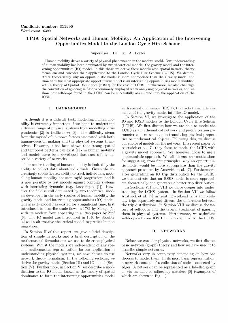
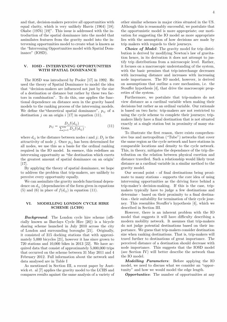
Networks vary in complexity depending on how onechooses to model them. In its most basic representation,a network consists of a collection of nodes connected byedges. A network can be represented as a labelled graphor via incident or adjacency matrices [8] (examples ofwhich are shown in Fig. 1).

2

5

1

2

3

4

(a) Simple Network

5

1

2

3

4

(b) Directed networkwith multi-edges

5

1

2

3

4

10

12

3

41

1

7

4

(c) Directed networkwith weighted edges

0 1 1 0 11 0 1 1 11 1 0 1 00 1 1 0 01 1 0 0 0

(d) Adjacencymatrix for (a)

1 2 0 0 00 0 1 1 00 0 1 3 00 1 0 0 01 1 0 0 0

(e) Adjacencymatrix for (b)

3 4 0 0 00 0 1 1 00 0 1 7 00 4 0 0 010 12 0 0 0

(f) Adjacency matrix

for (c)

FIG. 1: Various networks represented graphical and by cor-responding adjacency matrices. (a) A simple graph i.e. agraph that is undirected, unweighted, has no multi-edges andno self loops. (b) A non simple graph with multi-edges andself-loop. (c) A non simple weighted graph, where each edgelabel represent the weight of the edge. (d) Adjacency matrixrepresentation of graph shown in (a). (e) Adjacency matrixrepresentation of graph shown in (b). (f) Adjacency matrixrepresentation of graph shown in (c).

Two nodes are considered “adjacent” if an edge con-nects them. From this we can define the adjacent matrixas:

Aij = n, (1)

where n is the number of edges connecting node i to nodej. Incident matrix representation is an analogous repre-sentation where we consider two edges to be “incident” ifa node connects them. Incident matrix representation isof little interest in physical application where edges arenot well-defined, as is the case of the LCHS.

Furthermore, networks are sub-classified as directedand undirected. A directed network is where flows arerestricted to a single direction across edges, and undi-rected are where flows are bidirectional along edges. Notethat adjacency matrices for undirected networks must besymmetric, and for networks with no multi-edges the ad-jacency matrix is only populated with 0s and 1s. Werestrict our discussion to undirected networks with nomulti-edges.

Before being able to understand the trip-distributionmodels, we must first choose how we define three im-portant network characteristics, node importance, edgelength and self-edges.

Node Importance : In most physical networks, thenodes are not equal. This inequality is due to either cer-tain zones experiencing greater flows or, certain zones be-ing more “well connected” than others (e.g. some nodeshave greater numbers of edges originating from them).

One can use measures of node importance to help char-acterise these differences.

There are many ways of measuring node importance.The simplest definition is to define a node’s importanceas its “population”. In the case of a city, this could be thehuman population; or in the case of a traffic network, thiscould be the number of trips originating or terminatingat the zone. More complicated definitions define this as afunction of other parameters. For example, we will laterdefine node importance as a function of time of day whenapplying models to the LCHS.Edge Length : In any network, nodes are connected by

edges, and these do not remain uniform between differentzone pairs. This is of great importance when consideringspatial networks as edge length is often used to representthe topography of the surface the network is embedded.

There are a variety of ways of transforming physicalconnections between nodes to the mathematical edgesthat we need to model. Simple definitions include a linearrelationship of Euclidean distance between pairs of zonesto their respective edge length, whereas more complexdefinitions account for specific characteristics of routingdistances and factors that affect journey time.

Self-Edges (Self-Loops): Self-edges, also known asself-loops, occur when an edge connects a node to itself.They are represented by non-zero elements in the diago-nal of the adjacency matrix A (see Fig.1) Self-loops canbe very problematic in understanding spatial networks.Most investigations ignore self-loops, as either the flowsthrough the loops are small compared to the non-zeronon-diagonal elements of A, or they will not mathemati-cally affect parameters being calculated. Further, in thecase of the LCHS, due to the method of tracking used,they make it very difficult to properly model the network.At first, we will ignore self-loops in our application to theLCHS, but we will return to them later in Section VIII.

III. THE GRAVITY MODEL

As its name suggests, the gravity model is based onthe functional form of the Newton’s law of Gravitation.Gravity-law based models appear in a variety of socialand natural sciences, and human mobility is no excep-tion. The gravity model has been used to describe tripdistributions from as early as the 18th century by Monge[5]. The way in which it is presented today can be tracedback to Voorhees’ application of the gravity model totraffic in urban areas [9].

The gravity model states that the trip-interchange be-tween two nodes is directly proportional to the attrac-tion between the two nodes and inversely proportionallyto some function of the spatial separation between thenodes. The model assumes trip makers will aim to min-imise the ‘cost’ of a trip. The “cost” of a trip is usuallya function of spatial separation that also contains theinformation on other parameters that affect the trip dis-tribution [9].

3

To derive the gravity model for trip distribution, wefirst consider the gravity model of Newtonian physicsthat relates the force, Fij , between objects i and j, tothe objects masses, mi and mj , and the respective sepa-ration, dij , between the bodies:

Fij = Gmimj

d2ij, (2)

By analogy, we take equation (2) and make the followingchanges to instead predict the number of trips, Tij , be-tween mi and mj . Consider i and j as nodes instead ofbodies; replace the mi term with Oi, where Oi representsthe number of trips originating from node i; replace themj term with Dj , where Dj represents the number oftrips that terminate at node j; replace the dependence

of dij with a cost friction factor, Cβij (where β is some

constant, which is measures empirically) that is designedto incorporate the distance between the zones and anyother parameters that affect the trip distribution. Thisgives:

Tij = θOiDj

Cβij, (3)

where θ is some proportionality constant.A more general form of the gravity model is given as:

Tij =OiDjf(Cij)Kij∑nDn(Cin)Kin

, (4)

where Kij are “zone-to-zone adjustment factors”, Kij .Although originally introduced with no theoretical basis,attempts have been made to attribute them to “socioeco-nomic influences on travel otherwise unaccounted for inthe model” [15]. Derivation of equation (4) from (3) canbe seen in appendix A. There are two commonly usedfunctions for f(Cij):

f(Cij) = C−βij , (5)

f(Cij) = exp(−βCij), (6)

Equation (6), known as the “doubly constrained gravitymodel” [10], was initially derived by Wilson [11] to solvethe divergence issue that occurs with equation (5) forsmall values of Cij .

IV. THE INTERVENING OPPORTUNITIES(IO) MODEL

The opportunistic approach to modelling networks wasfirst proposed by Stouffer [4], who applied this approachto migration patterns between services and residences.The theory was further developed by Schneider [12] tothe general framework that is used today.

The law of intervening opportunities as proposed byStouffer [4] states “The number of persons going a given

distance is directly proportional to the number of oppor-tunities at that distance and inversely proportional to thenumber of intervening opportunities.” An “opportunity”is a destination that a trip-maker considers as a possibletermination point for their journey and an “interveningopportunity” is an opportunity that is closer to the tripmaker than the final destination but is rejected by thetrip-maker [4]. Mathematically, we have:

Tij = kDj

Vj, (7)

where k is a proportionality constant, Dj represents thetotal number of opportunities at node j, and the quantityVj is the number of intervening opportunities betweennodes i and j.

Schneider proposed a modified Stouffer hypothesis [12]:“The probability that a trip will terminate in some vol-ume of destination points is equal to the probability thatthis volume contains an acceptable destination times theprobability that an acceptable destination closer to theorigin of the trips has not been found.”

This was represented mathematically by Ruiter [13] as

dP = L[1− P (V )]dV, (8)

where dP is the probability that a trip will terminatewhen considering dV possible destinations; the ‘sub-tended volume’ V is the cumulative total number of des-tination opportunities considered up to the destinationbeing considered; dV is an element of the subtended vol-ume at the surface of the volume; P (V ) represents theopportunity that a trip terminates when V destinationsare considered; L is a constant probability of a possibledestination being accepted if it is considered. The solu-tion of equation (8) is

P (V ) = 1− exp(−LV ), (9)

With the expected trip-interchange, Tij , we get

Tij = Oi[P (Vj+1)− P (Vj)], (10)

where Oi represents the total number of opportunitiesat node i. Note that Eash [14] showed that the gravityand IO models are “fundamentally the same” and areboth derivable from entropy maximization theory. Eashalso noted that the difference is how the “cost” of travelis considered [14]. Although the gravity model consid-ers this “cost’ as a function of distance, the opportunitymodel considers the “cost” as the difficulty to satisfy atrip’s purpose. The gravity model then treats the dis-tance variable as a continuous cardinal variable, whilstthe opportunity model treats the distance as an ordinalvariable.

At this juncture it is necessary to recognise the ma-jor shortcoming of the conventional intervening oppor-tunities model. As described by Pooler [16]: ”Themodel implies that the linear distance between nodeshas no direct effect on the perception of opportunities,

4

and that, decision-makers perceive all opportunities withequal clarity, which is very unlikely Harris (1964) [18];Okabe (1976) [19]”. This issue is addressed with the in-troduction of the spatial dominance into the model thatassimilates features from the gravity model into the in-tervening opportunities model to create what is known asthe “Intervening Opportunities model with Spatial Dom-inance” (IOSD).

V. IOSD - INTERVENING OPPORTUNITIESWITH SPATIAL DOMINANCE

The IOSD was introduced by Pooler [17] in 1992. Heused the theory of Spatial Dominance to model the ideathat “decision-makers are influenced not just by the sizeof a destination or distance but rather by these two fac-tors in combination”. To do this, one applies the func-tional dependence on distance seen in the gravity basedmodels to the ranking process of the intervening models.We define the“theoretical spatial dominance”, pij of adestination j on an origin i [17] in equation (11).

pij =Djf(dij)∑mj=1Djf(dij)

, (11)

where dij is the distance between nodes i and j; Dj is theattractivity of node j. Once pij has been determined forall nodes, we use this as a basis for the ordinal rankingrequired in the IO model. In essence, this redefines anintervening opportunity as “the destination which exertsthe greatest amount of spatial dominance on an origin’[17].

By applying the theory of spatial dominance, we hopeto address the problem that trip-makers, are unlikely toperceive every opportunity equally.

We can assimilate the gravity models functional depen-dence on dij (dependancies of the form given in equations(5) and (6) in place of f(dij) in equation (11).

VI. MODELLING LONDON CYCLE HIRESCHEME (LCHS)

Background : The London cycle hire scheme (offi-cially known as Barclays Cycle Hire [20]) is a bicyclesharing scheme launched in July 2010 across the cityof London and surrounding boroughs [21]. Originally,it consisted of 315 docking stations that with approxi-mately 5,000 bicycles [21], however it has since grown to720 stations and 10,000 bikes in 2013 [22]. We have ac-quired data that consist of approximately 5,000,000 tripsthat occurred on the scheme between 31 May 2011 and 4February 2012. Full information about the network anddata analysed are in Table I

As mentioned in Section III, a recent paper by Aust-wick et. al [7] applies the gravity model to the LCHS andcompares results against the same analysis of a variety of

other similar schemes in major cities situated in the US.Although this is reasonably successful, we postulate thatthe opportunistic model is more appropriate; our moti-vation for suggesting the IO model as more appropriatelies with the assumption of how decisions are made bytrip makers with regards to their journeys.Choice of Model : The gravity model for trip distri-

bution is derived by modifying Newton’s law of gravita-tion hence, in its derivation it does not attempt to jus-tify trip distributions from a microscopic level. Rather,it focuses on a macroscopic understanding of the system,with the basic premises that trip-interchange decreaseswith increasing distance and increases with increasingnode importances. The IO model, however, is derivedon assumptions that outline a core mechanism, i.e. theStouffer hypothesis [4], that drive the macroscopic prop-erties of the system.

Furthermore, we postulate that trip-makers do notview distance as a cardinal variable when making theirdecisions but rather as an ordinal variable. Our rationaleis based on two facts: trip-makers are not restricted tousing the cycle scheme to complete their journeys; trip-makers likely have a final destination that is not situatedexactly at a single station but in proximity of many sta-tions.

To illustrate the first reason, there exists comprehen-sive bus and metropolitan (“Tube”) networks that coverthe same region as the cycle network and have stations incomparable locations and density to the cycle network.This, in theory, mitigates the dependance of the trip dis-tribution on the relation between physical exertion anddistance travelled. Such a relationship would likely treatdistance as a cardinal variable in a similar method to thegravity model.

Our second point - of final destinations being proxi-mate to many stations - supports the core idea of usingintervening opportunities as the driving force behind atrip-maker’s decision-making. If this is the case, trip-makers typically have to judge a few destinations anddetermine - based on their proximity to a final destina-tion - their suitability for termination of their cycle jour-ney. This resembles Stouffer’s hypothesis [4], which wedescribed in Section III.

However, there is an inherent problem with the IOmodel that suggests it will have difficulty describing amodern mobility network. It assumes that trip-makersdo not judge potential destinations based on their im-portance. We guess that trip-makers consider destinationsize when ranking destinations. That is, trip-makers willtravel further to destinations of great importance. Theperceived distance of a destination should decrease withnode importance. This suggests that the IOSD model(see Section IV) will better describe the network thanthe IO model.Modelling Parameters: Before applying the IO

model, we need to discuss what we consider an “oppor-tunity” and how we would model the edge length.Opportunties: The number of opportunities at any

5

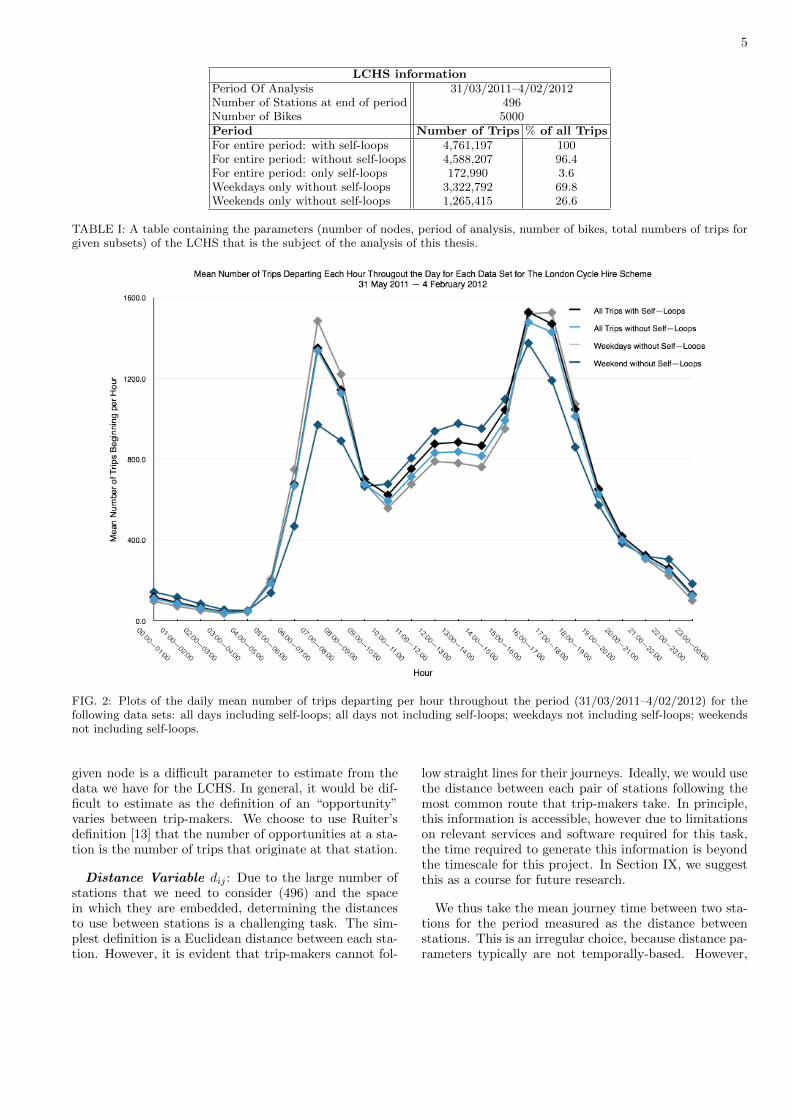
LCHS informationPeriod Of Analysis 31/03/2011–4/02/2012Number of Stations at end of period 496Number of Bikes 5000Period Number of Trips % of all TripsFor entire period: with self-loops 4,761,197 100For entire period: without self-loops 4,588,207 96.4For entire period: only self-loops 172,990 3.6Weekdays only without self-loops 3,322,792 69.8Weekends only without self-loops 1,265,415 26.6

TABLE I: A table containing the parameters (number of nodes, period of analysis, number of bikes, total numbers of trips forgiven subsets) of the LCHS that is the subject of the analysis of this thesis.

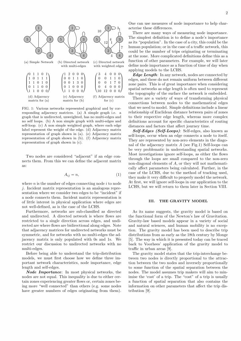
FIG. 2: Plots of the daily mean number of trips departing per hour throughout the period (31/03/2011–4/02/2012) for thefollowing data sets: all days including self-loops; all days not including self-loops; weekdays not including self-loops; weekendsnot including self-loops.

given node is a difficult parameter to estimate from thedata we have for the LCHS. In general, it would be dif-ficult to estimate as the definition of an “opportunity”varies between trip-makers. We choose to use Ruiter’sdefinition [13] that the number of opportunities at a sta-tion is the number of trips that originate at that station.

Distance Variable dij : Due to the large number ofstations that we need to consider (496) and the spacein which they are embedded, determining the distancesto use between stations is a challenging task. The sim-plest definition is a Euclidean distance between each sta-tion. However, it is evident that trip-makers cannot fol-

low straight lines for their journeys. Ideally, we would usethe distance between each pair of stations following themost common route that trip-makers take. In principle,this information is accessible, however due to limitationson relevant services and software required for this task,the time required to generate this information is beyondthe timescale for this project. In Section IX, we suggestthis as a course for future research.

We thus take the mean journey time between two sta-tions for the period measured as the distance betweenstations. This is an irregular choice, because distance pa-rameters typically are not temporally-based. However,

6

the models do not require that the distance parametermust be a spatial one. Furthermore, journey time con-tains relevant information, that we argue makes meanjourney time a more appropriate a metric than physicaldistance. This is largely due to the idea that trip makersare likely to be sensitive to journey time, and that traf-fic effects are likely to change the “perceived distance”between nodes. Furthermore, this allows us to considerchanging edge lengths (that are functions of time of day).

Austwick et. al took the approach of using Eu-clidean/Great Circle distances as edge lengths as, in theiropinion, “Euclidean/Great Circle distance is at least freefrom these additional assumptions”, where “these addi-tional assumptions” refer to assumptions that would haveto be made if routing information was used instead. Ouruse of mean journey time would also be subject to simi-lar assumptions. However, this is not as great a problemas we are using an opportunistic model where we treatdistance as ordinal rather than cardinal i.e. since we donot care about the absolute values of distances betweennodes (rather we only care about the relative order ofdistance length) we are able to make assumptions aboutedge length as long as they do not greatly affect the rank-ings of destinations.

Model results: Given the definitions for the oppor-tunities of each node and the edge length between eachpair of nodes, we can now analyse the data to determinethe nature of the trip distributions and compare againstthe results found by Austwick et. al.

When applying our model, we to consider the networkat each hour of the day. We split our data into hoursets by considering only trips that departed their originin that hour. We calculated the mean journey time be-tween each pair of nodes and created a ranking matrixthat ranked destinations, j, for each origin, i, based uponthe “temporal distance” between them. We then followthe theory given in Section IV for the IOs model to deter-mine the probability, P (V ), of a trip terminating, after Vopportunities are considered. Then the probability is ob-tained by dividing the number of trips occurring againstthe total number of trips.

When fitting distributions to the data, we applieda nonlinear least-squares method Mathworks MatlabCurve Fitting ToolboxTM[23]. The methodology behindthe fit is given in Appendix B.

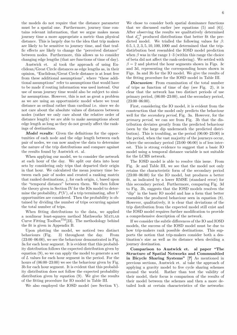
Upon plotting the model, we noticed two distinctbehaviours (Fig. 3) throughout the day. From(23:00–06:00), we see the behaviour demonstrated in Fig.3a for each hour segment. It is evident that this probabil-ity distribution follows the expected distribution given byequation (9), so we can apply the model to generate a setof L values for each hour segment in the period. For thehours of (06:00–23:00) we see the behaviour given by Fig.3b for each hour segment. It is evident that this probabil-ity distribution does not follow the expected probabilitydistribution given by equation (9). We give the resultsof the fitting procedure for IO model in Table III.

We also employed the IOSD model (see Section V).

We chose to consider both spatial dominance functionsthat we discussed earlier [see equations (5) and (6)].After observing the results we qualitatively determinedthat d−bij produced distributions that better fit the pre-dicted model. We trialled the following values for β:0.5, 1, 2, 3, 5, 10, 100, 1000 and determined that the trip-distirbution best resembled the IOSD model predictionwhen β was in the range 1–3 (within this range the choiceof beta did not affect the rank-ordering). We settled withβ = 2 and plotted the hour segments shown in Figs. 3cand 3d, representing the corresponding hours shown inFigs. 3a and 3b for the IO model. We give the results ofthe fitting procedure for the IOSD model in Table III.

Discussion : From examination of the total numberof trips as function of time of day (see Fig. 2), it isclear that the network has two distinct periods of useprimary period, (06:00–23:00), and the secondary period,(23:00–06:00).

First, considering the IO model, it is evident from theconstruction that the model only predicts the behaviourwell for the secondary period, Fig. 3a. However, for theprimary period, we can see from Fig. 3b that the dis-tribution deviates greatly from the predicted behaviour(seen by the large dip underneath the predicted distri-bution). This is troubling, as the period (06:00–23:00) isthe period, when the vast majority of the journeys occur,where the secondary period (23:00–06:00) is of less inter-est. This is strong evidence to suggest that a basic IOmodel using a temporal distance variable is not suitablefor the LCHS network.

The IOSD model is able to resolve this issue. FromFig. 3c and Table III, we see that the model not onlyretains the characteristic form of the secondary period(23:00–06:00) for the IO model, but produces a betterfit, as indicated by a lower RMSE (standard error) forthis secondary period. Furthermore, comparing Fig. 3dto Fig. 3b, suggests that the IOSD models resolves the“dip” in the basic IO model and has a form that betterresembles the produced behaviour seen in equation (8).However, qualitatively, it is clear that deviations of thetrip distribution from the expected model still exist andthe IOSD model requires further modification to providea comprehensive description of the network.

If we consider the subtle differences of the IO and IOSDmodels, the success of the IOSD model must be due tohow trip-makers rank possible destinations. This sup-ports the notion that trip-makers consider both a des-tination’s size as well as its distance when deciding ajourney destination.

Comparison to Austwick et. al paper “TheStructure of Spatial Networks and Communitiedin Bicycle Sharing Systems” [7] As mentioned inprevious sections, Austwick et. al take the approach ofapplying a gravity model to five cycle sharing schemesaround the world. Rather than test the validity oftheir model, their focus is comparison of the results oftheir model between the schemes and then a more de-tailed look at certain characteristics of the networks:

7

(a) (b)

(c) (d)

FIG. 3: Plots of the probability distributions for both IO and IOSD models representing the two behaviours demonstrated bythe models. (a) IO model plot of hour (01:00–02:00) demonstrating the general behaviour of network in the period (23:00–06:00).(b) IO model plot of hour (16:00–17:00) demonstrating the general behaviour of network in the period (06:00–23:00). (c) IOSDmodel equivalent plot of (a). (d) IOSD model equivalent plot of (b).

time-dependance; seasonality; detection of communities(“subregions within the bike sharing flow networks whichare linked to one another more strongly than nodesfrom other subregions”). Furthermore, Austwick et. al.choose to use a Euclidean/Great Circle method for cal-culating distances.

Austwick et. al are able to show that all the schemesthey analysed behave similarly, with trip distributionsbearing reasonable similarity. They show the overallshape of the “probability mass function of journeys”(probability distribution function of trips made againstEuclidean distances) is consistent between schemes, butthere exists a large deviation between the networks thatsuggests that a better model exists for cycle schemes.Furthermore, their calculated model’s dependance on dis-tance is not a standard functional dependance as wewould expect from the gravity model (see equations 5and 6).

In comparison, although our model suffers similarproblems, we are able to generate trip distributions ofthe overall functional form expected of our IOSD model.However, during the secondary period, the data clearlydeviates from the expected model. Our IOSD model re-sults offer a slight improvement in that we are able tofit the standard form for the IOSD model to our tripdistribution.

Furthermore, we have been able to show our modelis viable, whilst using a more complex distance variablethan Austwick et al. Our use of mean journey time overEuclidean distance is preferable as it includes the effect ofother important characteristics of the cycle hire schemes,namely traffic conditions.

There are a few factors that might be the cause of thediscrepancies between the IO and IOSD models. Themore likely issue is the use of “mean journey time”as the distance variable. However, as we have seen in

8

Network Characteristics Number of Trips Number of EdgesWith Self-Loops Without Self-Loops With Self-Loops Without Self-Loops

Hour of Day Everyday Everyday Weekdays Only Weekends Only Everyday Everyday Weekdays Only Weekends Only“Primary Period” (06:00–23:00)

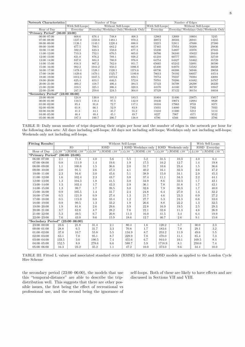
06:00–07:00 668.6 676.4 748.8 468.3 12963 12669 10604 524507:00–08:00 1337.0 1350.6 1484.1 970.2 30872 30503 26941 1424508:00–09:00 1126.1 1143.1 1220.4 890.8 53215 52811 47688 2738009:00–10:00 677.5 700.5 682.2 665.8 57465 57054 50209 2983610:00–11:00 592.2 623.3 558.0 677.3 55230 54807 45976 2794511:00–12:00 713.3 752.1 676.5 805.0 56766 56340 45822 2944912:00–13:00 831.8 876.2 789.1 938.2 61210 60777 50051 3274913:00–14:00 837.0 884.3 780.9 976.8 64754 64327 53462 3572914:00–15:00 816.3 867.2 762.0 951.7 65665 65242 53891 3659015:00–16:00 992.2 1044.2 950.3 1096.8 65400 64970 53582 3603816:00–17:00 1478.4 1528.1 1520.1 1374.6 68736 68308 56946 3905817:00–18:00 1429.6 1470.1 1525.7 1189.8 78613 78192 68057 4451418:00–19:00 1012.3 1047.5 1073.6 859.5 79754 79337 70394 4209119:00–20:00 625.4 653.1 646.5 572.8 70701 70286 61682 3476720:00–21:00 400.2 418.7 406.4 384.5 57123 56708 28298 2622021:00–22:00 310.5 325.1 306.4 320.8 44570 44160 36739 1894722:00–23:00 247.3 259.6 224.5 304.0 37529 37122 30154 16034

“Secondary Period” (23:00–06:00)23:00–00:00 124.8 130.8 101.3 183.5 31804 31406 23875 1501700:00–01:00 110.5 118.4 97.5 142.9 19440 19074 12884 982801:00–02:00 85.4 91.0 72.7 117.1 18316 17963 9733 837102:00–03:00 61.8 66.1 52.9 83.9 15031 14680 7502 703303:00–04:00 41.3 44.1 35.7 55.3 11610 11300 5212 511304:00–05:00 46.4 48.4 45.1 49.7 8227 7967 4571 353205:00–06:00 187.3 190.7 206.7 138.8 6796 6566 10604 2786

TABLE II: Daily mean number of trips departing their origin per hour and the number of edges in the network per hour forthe following data sets: All days including self-loops; All days not including self-loops; Weekdays only not including self-loops;Weekends only not including self-loops.

Fitting Results Without Self-Loops With Self-LoopsIO IOSD IOSD Weekdays only IOSD Weekends only IOSD Everyday

Hour of Day L(10−5) RMSE (10−5) L(10−5) RMSE (10−3) L(10−5) RMSE (10−5) L(10−5) RMSE (10−5) L(10−5) RMSE (10−5)“Primary Period” (06:00–23:00)

06:00–07:00 2.1 71.3 4.0 5.6 5.5 5.2 31.5 10.3 4.0 6.407:00–08:00 0.8 111.9 1.4 19.6 1.9 17.5 10.2 12.7 1.4 19.808:00–09:00 1.1 100.8 1.5 36.6 2.0 31.7 10.6 23.4 1.5 36.609:00–10:00 2.0 91.5 2.6 47.3 4.1 40.2 16.1 32.3 2.6 47.210:00–11:00 2.3 94.6 3.0 45.6 5.1 38.9 15.0 34.1 2.9 45.311:00–12:00 1.6 102.4 2.3 43.7 3.8 37.4 11.1 34.3 2.2 44.112:00–13:00 1.3 104.3 1.8 41.5 3.0 34.9 8.6 32.3 1.7 42.113:00–14:00 1.3 102.4 1.7 42.3 2.9 36.1 7.8 31.8 1.7 42.114:00–15:00 1.3 99.7 1.7 39.5 3.0 32.6 7.9 30.3 1.7 40.015:00–16:00 0.9 105.5 1.4 31.7 2.4 24.8 6.4 27.0 1.4 32.216:00–17:00 0.5 121.9 0.9 27.4 1.3 21.7 4.6 23.3 0.9 27.217:00–18:00 0.5 115.9 0.8 33.4 1.2 27.7 5.3 24.3 0.8 33.018:00–19:00 0.9 99.5 1.3 33.2 1.9 26.6 8.8 22.2 1.3 32.519:00–20:00 1.9 81.8 2.6 29.6 3.9 22.8 16.9 19.5 2.5 29.320:00–21:00 3.7 62.8 4.7 28.2 7.6 22.1 32.6 11.3 4.6 26.921:00–22:00 5.3 49.5 6.7 20.8 11.3 16.0 41.5 3.4 6.4 19.922:00–23:00 7.6 43.0 9.6 15.9 18.6 12.7 46.7 2.6 9.1 15.6

“Secindary Period” (23:00–06:00)23:00–00:00 23.6 21.8 31.4 2.1 80.4 1.6 120.2 5.7 30.0 2.300:00–01:00 28.8 6.5 31.7 3.3 70.8 1.7 183.6 7.8 29.1 3.201:00–02:00 37.0 10.7 55.8 5.5 134.9 8.7 253.2 11.9 49.6 5.502:00–03:00 63.1 7.0 95.1 8.7 229.9 7.8 470.0 11.1 85.4 7.303:00–04:00 133.5 3.0 190.5 7.4 455.6 6.7 944.0 10.1 169.5 8.404:00–05:00 152.5 8.8 278.6 6.6 580.7 5.9 1718.9 8.1 250.0 7.405:00–06:00 16.3 23.2 35.2 1.1 47.2 10.0 373.0 9.6 34.4 10.0

TABLE III: Fitted L values and associated standard error (RMSE) for IO and IOSD models as applied to the London CycleHire Scheme

the secondary period (23:00–06:00), the models that usethis “temporal-distance” are able to describe the trip-distribution well. This suggests that there are other pos-sible issues, the first being the effect of recreational vsprofessional use, and the second being the ignorance of

self-loops. Both of these are likely to have effects and arediscussed in Sections VII and VIII.

9

VII. WEEKDAY VS WEEKEND USE

Following the example of Austwick et. al, we investi-gate the difference between weekday and weekend use.We predict a difference between trip distributions forweekdays and weekends to reflect that we expect greatercommuter use during weekdays and greater leisure use atthe weekend.

Examination of Fig. 2 (daily mean of number of tripsdeparting their origin per hour for different data sets)demonstrates there is a difference in use of the LCHSbetween weekdays and weekends.

Both data sets show two peaks in trip numbersduring the same hours of the day (04:00–10:00) and(16:00–21:00). Weekends have maxima at (07:00–08:00)and (16:00–17:00), whilst weekdays have maxima at(07:00–08:00) and (17:00–18:00). Furthermore, the week-day peaks are equally tall and both wider and taller thanthe corresponding weekend peaks. This supports the no-tion that weekday use of the LCHS is dominated by com-muter use, as the peaks are situated at the hours directlybefore and after the working day (typically 09:00–17:00).Furthermore, the morning peak for weekend use is 30%smaller than the afternoon peak, and during periods be-tween peaks (07:00–08:00) and (16:00–17:00), there isgreater use than that seen during weekdays. The combi-nation of these, provides evidence the idea of commuteruse being less dominant during weekends.

We applied the IOSD model via the same method asapplied to the full data set, detailed in section VI. Fittingresults of this process for both weekdays and weekendsare given in Table III, whilst plots of the total number oftrips as a function of hour of day are give in Fig. 2.

As in Section VI, we examined the fits and were ableto determine that the behaviour of the network for bothweekday use and weekend use were not qualitatively dif-ferent from the the overall network use. For both datasets there is a clear difference in behaviour during the“primary period” (06:00–23:00) and “secondary period”(23:00–06:00). Furthermore, there was little differencebetween weekday and weekend use, beyond the differ-ence in total trip use throughout the day, as discussed inthe previous paragraph.

This leads us to conclude that beyond evidence ofgreater commuter use during the weekday morning pe-riod, the network can be modelled similarly throughoutthe week.

VIII. SELF-LOOPS

We will now return to discussing self-loops. As dis-cussed in Section II, self-loops are situations where anedge connects a node directly to itself, represented as anon-zero diagonal element in the adjacency matrix. Theyare difficult to understand in physical systems where weonly have origin-destination data on trip-makers, as is thecase of the LCHS. With typical treatment of journeys,

they appear as journeys for which the distance dij = 0.Application of a zero dij to the standard gravity model(5) provides a nonsensical result due to the divergence ofthe model as dij approaches zero.

Choosing to ignore self-loops when applying networktheory is typically used as a solution as often flows alongself-loops are small compared to flows along other edges.In Austwick et. al’s paper [7] on cycle hire schemes, theytake this approach with the justification that “displace-ments are not reasonably calculable for these journeys”[7].

In prior sections, we took the same approach as Aust-wick et. al in our treatment of self-loops. Self-loops con-stitute 3.6% (see Table I) and thus cannot be consid-ered insignificant for this network. Therefore, our IOSDmodel without self-loops provides an incomplete under-standing of the network as a whole and needs to be ad-dressed.

Typically, we are unable to assimilate self-loops intostandard gravity models and IO models, as the availabledata does not allow us to know the edge length of anytrip that starts and ends at the same destination. How-ever, our choice of using mean journey time as the edgelength offers a solution to this problem. Using the sametreatment for self-loops as we have for the rest of the net-work, we model each node’s self-loop with an edge lengthequal to the mean journey time for all self-loop trips andthen follow the steps detailed in Section V.

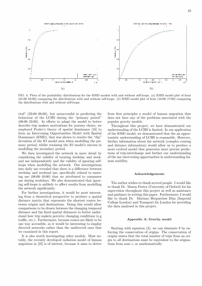
Using the IOSD model (as used in Section VI), the fit-ted results of the modelling of the network are shownin Table III and the self-loop distributions for hours(01:00–02:00) and (16:00–17:00) are shown in Fig. 4aand 4b, alongside the distributions without self-loops in-cluded.

From Fig. 4, we observe that our inclusion of self-loops with identical treatment to the other trips doesnot cause any significant deviation from the distributionswithout self-loops. Furthermore, the small difference offitted L values between with and without self-loops datasets (see Table III), this suggest that self-loops do not af-fect the trip-distributions greatly and ignoring self-loopsis a reasonable approach when attempting to understandthe global properties of the network. However, the differ-ence supports our premise that self-loops are relevant fora complete understanding go the system. In summary,the exclusion of self-loops causes an our model to under-estimate the probability that a trip will terminate whena trip makers considers an opportunity.

IX. SUMMARY

The aim of this project was to assess the suitabilityof the intervening opportunity (IO) model as an alter-native to the gravity model for describing human mobil-ity patterns seen in the LCHS. By applying the model,we showed that the IO model can successfully modelthe trip distribution during the daily “secondary pe-

10

(a) (b)

FIG. 4: Plots of the probability distributions for the IOSD models with and without self-loops. (a) IOSD model plot of hour(01:00–02:00) comparing the distributions with and without self-loops. (b) IOSD model plot of hour (16:00–17:00) comparingthe distributions with and without self-loops.

riod” (23:00–06:00), but unsuccessful in predicting thebehaviour of the LCHS during the “primary period”(06:00–23:00). In efforts to adapt the model to betterdescribe trip makers motivations for journey choice, weemployed Pooler’s theory of spatial dominance [16] toform an Intervening Opportunities Model with SpatialDominance (IOSD), that was shown to resolve the “dip”deviation of the IO model seen when modelling the pri-mary period, whilst retaining the IO model’s success inmodelling the secondary period.

We then investigated the network in more detail byconsidering the validity of treating weekday and week-end use independently and the validity of ignoring self-loops when modelling the network. Our investigationsinto daily use revealed that there is a difference betweenweekday and weekend use, specifically related to morn-ing use (08:00–10:00) that we attributed to commuteruse during weekdays. We also demonstrated that ignor-ing self-loops is unlikely to affect results from modellingthe network significantly.

For further investigations, it would be most interest-ing from a theoretical perspective to produce a spatialdistance matrix that represents the shortest routes be-tween origins and destinations. Doing this would allowcomparisons to be drawn between the changing temporaldistance and the fixed spatial distances to better under-stand how trip makers perceive changing conditions (e.gtraffic, etc.). Furthermore, because routes are likely to beone way accessible, so it would be interesting to employdirected networks rather than the undirected ones thatwe examined in this report.

It is also worth investigating other models. Most no-tably, the recently developed radiation model of humanmigration in [25] is of interest, because it aims to derive

from first principles a model of human migration thatdoes not have any of the problems associated with thepopular gravity models.

Throughout this project, we have demonstrated ourunderstanding of the LCHS is limited. In our applicationof the IOSD model, we demonstrated that the an oppor-tunistic understanding of LCHS is reasonable. However,further information about the network (complex routingand distance information) would allow us to produce amore evolved model that generates more precise predic-tions of trip-interchange and further our understandingof the use intervening opportunities in understanding hu-man mobility.

Acknowledgements

The author wishes to thank several people. I would liketo thank Dr. Mason Porter (University of Oxford) for hissupervision throughout this project as well as assistanceand guidance in writing this paper. Furthermore, I wouldlike to thank Dr. Mariano Berguerisse Dıaz (ImperialCollege London) and Transport for London for providingthe data analysed in this project.

Appendix A: Gravity model

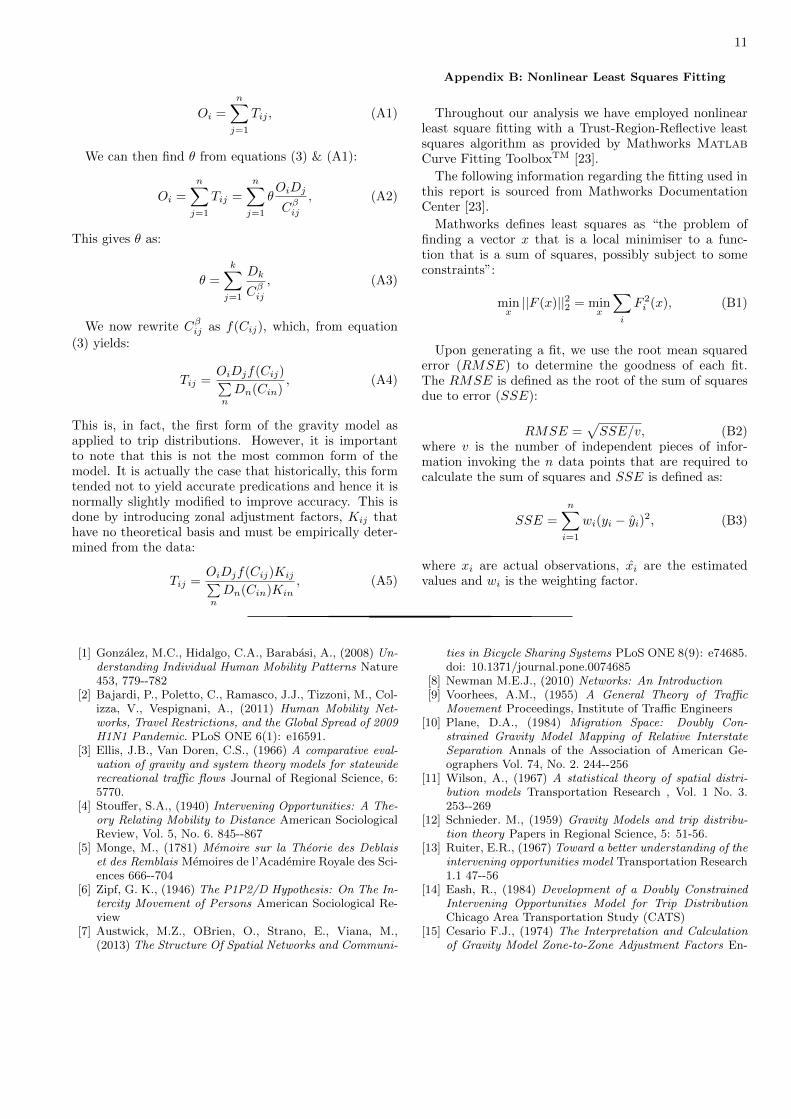
Starting with equation (3), we can eliminate θ by en-forcing the conservation of origins. The conservation oforigins states that the total number of trips from an ori-gin to all destinations must be equivalent to the origina-tions from zone i, or mathematically

11

Oi =

n∑j=1

Tij , (A1)

We can then find θ from equations (3) & (A1):

Oi =

n∑j=1

Tij =

n∑j=1

θOiDj

Cβij, (A2)

This gives θ as:

θ =

k∑j=1

Dk

Cβij, (A3)

We now rewrite Cβij as f(Cij), which, from equation

(3) yields:

Tij =OiDjf(Cij)∑nDn(Cin)

, (A4)

This is, in fact, the first form of the gravity model asapplied to trip distributions. However, it is importantto note that this is not the most common form of themodel. It is actually the case that historically, this formtended not to yield accurate predications and hence it isnormally slightly modified to improve accuracy. This isdone by introducing zonal adjustment factors, Kij thathave no theoretical basis and must be empirically deter-mined from the data:

Tij =OiDjf(Cij)Kij∑nDn(Cin)Kin

, (A5)

Appendix B: Nonlinear Least Squares Fitting

Throughout our analysis we have employed nonlinearleast square fitting with a Trust-Region-Reflective leastsquares algorithm as provided by Mathworks MatlabCurve Fitting ToolboxTM [23].

The following information regarding the fitting used inthis report is sourced from Mathworks DocumentationCenter [23].

Mathworks defines least squares as “the problem offinding a vector x that is a local minimiser to a func-tion that is a sum of squares, possibly subject to someconstraints”:

minx||F (x)||22 = min

x

∑i

F 2i (x), (B1)

Upon generating a fit, we use the root mean squarederror (RMSE) to determine the goodness of each fit.The RMSE is defined as the root of the sum of squaresdue to error (SSE):

RMSE =√SSE/v, (B2)

where v is the number of independent pieces of infor-mation invoking the n data points that are required tocalculate the sum of squares and SSE is defined as:

SSE =

n∑i=1

wi(yi − yi)2, (B3)

where xi are actual observations, xi are the estimatedvalues and wi is the weighting factor.

[1] Gonzalez, M.C., Hidalgo, C.A., Barabasi, A., (2008) Un-derstanding Individual Human Mobility Patterns Nature453, 779--782

[2] Bajardi, P., Poletto, C., Ramasco, J.J., Tizzoni, M., Col-izza, V., Vespignani, A., (2011) Human Mobility Net-works, Travel Restrictions, and the Global Spread of 2009H1N1 Pandemic. PLoS ONE 6(1): e16591.

[3] Ellis, J.B., Van Doren, C.S., (1966) A comparative eval-uation of gravity and system theory models for statewiderecreational traffic flows Journal of Regional Science, 6:5770.

[4] Stouffer, S.A., (1940) Intervening Opportunities: A The-ory Relating Mobility to Distance American SociologicalReview, Vol. 5, No. 6. 845--867

[5] Monge, M., (1781) Memoire sur la Theorie des Deblaiset des Remblais Memoires de l’Academire Royale des Sci-ences 666--704

[6] Zipf, G. K., (1946) The P1P2/D Hypothesis: On The In-tercity Movement of Persons American Sociological Re-view

[7] Austwick, M.Z., OBrien, O., Strano, E., Viana, M.,(2013) The Structure Of Spatial Networks and Communi-

ties in Bicycle Sharing Systems PLoS ONE 8(9): e74685.doi: 10.1371/journal.pone.0074685

[8] Newman M.E.J., (2010) Networks: An Introduction[9] Voorhees, A.M., (1955) A General Theory of Traffic

Movement Proceedings, Institute of Traffic Engineers[10] Plane, D.A., (1984) Migration Space: Doubly Con-

strained Gravity Model Mapping of Relative InterstateSeparation Annals of the Association of American Ge-ographers Vol. 74, No. 2. 244--256

[11] Wilson, A., (1967) A statistical theory of spatial distri-bution models Transportation Research , Vol. 1 No. 3.253--269

[12] Schnieder. M., (1959) Gravity Models and trip distribu-tion theory Papers in Regional Science, 5: 51-56.

[13] Ruiter, E.R., (1967) Toward a better understanding of theintervening opportunities model Transportation Research1.1 47--56

[14] Eash, R., (1984) Development of a Doubly ConstrainedIntervening Opportunities Model for Trip DistributionChicago Area Transportation Study (CATS)

[15] Cesario F.J., (1974) The Interpretation and Calculationof Gravity Model Zone-to-Zone Adjustment Factors En-

12

vironment and Planning, Vol 6 247 --257[16] Pooler, J.A., (1992) Spatial Uncertainty and Spatial

Dominance in Interaction Modelling: A Theoretical Per-spective on Spatial Competition Environment and Plan-ning Vol. 24 995--1008

[17] Pooler, J.A., Akwawu, S., (2001) The development of anintervening opportunities model with spatial dominanceeffects J Geograph Syst 3:69--86

[18] Harris, B., (1964) A Note on the Probability of Interac-tion at a Distance Journal of regional Science 2(2): 31--35

[19] Okabe, A., (1976) Applied Models in Urban and RegionalAnalysis Prentice-Hall Inc. Englewood Cliff NJ

[20] 2010 Barclays’ 25m sponsorship of London cyclehire scheme BBC News, http://www.bbc.co.uk/news/

10182833 (5 April 2014)

[21] 2010 London saddles up for new bike hirescheme BBC News, http://www.bbc.co.uk/news/

uk-england-london-10810869 (5 April 2014)[22] 2010 Barclays Cycle Hire / Key Facts BBC

News, http://www.tfl.gov.uk/modes/cycling/

barclays-cycle-hire/find-a-docking-station?

intcmp=5386 (5 April 2014)[23] Curve Fitting Toolbox MathWorks http:

//www.mathworks.co.uk/help/curvefit/

product-description.html(5 April 2014)[24] Barthelemy, M. (2010)Spatial Networks Physics Reports

499:1--101[25] Simini, F., Gonza M.C., Maritan, A., Barabasi, A.,

(2012) A Universal Model For Mobility and MigrationPatterns Nature Vol. 484 96--100