TR 2010-136 A1b - Defence Research Reportscradpdf.drdc-rddc.gc.ca/PDFS/unc111/p535180_A1b.pdf · These echoes are processed using an automatic classiﬁer that quantiﬁes the timbre

DEFENCE DÉFENSE&

Defence R&D Canada – Atlantic

Copy No. _____

Defence Research andDevelopment Canada

Recherche et développementpour la défense Canada

Aural classification and temporal robustness

Stefan M. MurphyPaul C. Hines

Technical Report

DRDC Atlantic TR 2010-136

November 2010

This page intentionally left blank.


Stefan M. MurphyPaul C. Hines

Defence R&D Canada – AtlanticTechnical ReportDRDC Atlantic TR 2010-136November 2010

Principal Author

Original signed by Stefan M. Murphy

Stefan M. Murphy

Defence Scientist

Approved by

Original signed by Garry Heard for

Daniel Hutt Head/Underwater Sensing

Approved for release by

Original signed by Ron Kuwahara for

Calvin Hyatt

Head/Document Review Panel

© Her Majesty the Queen in Right of Canada, as represented by the Minister of National Defence, 2010

© Sa Majesté la Reine (en droit du Canada), telle que représentée par le ministre de la Défense nationale, 2010

Abstract

Active sonar systems are used to detect underwater manmade objects of interest (targets)

that are too quiet to be reliably detected with passive sonar. In coastal waters, the perfor-

mance of active sonar is degraded by false alarms caused by echoes returned from geo-

logical seabed structures (clutter) found in these shallow regions. To reduce false alarms,

a method of distinguishing target echoes from clutter echoes is required. Research has

demonstrated that perceptual signal features similar to those employed in the human audi-

tory system can be used to automatically discriminate between target and clutter echoes,

thereby improving sonar performance by reducing the number of false alarms.

An active sonar experiment on the Malta Plateau was conducted during the Clutter07 sea

trial and repeated during the Clutter09 sea trial. Broadband sources were used to transmit

linear FM sweeps (600–3400 Hz) and a cardioid towed-array was used as the receiver. The

dataset consists of over 95 000 pulse-compressed echoes returned from two targets and

many geological clutter objects.

These echoes are processed using an automatic classifier that quantifies the timbre of each

echo using a number of perceptual signal features. Using echoes from 2007, the aural

classifier is trained to establish a boundary between targets and clutter in the feature space.

Temporal robustness is then investigated by testing the classifier on echoes from the 2009

experiment.

Resume

Les sonars actifs servent a detecter sous l’eau des objets d’interet artificiels (cibles) trop

silencieux pour etre detectes efficacement par un sonar passif. En eaux cotieres, les echos

provenant de structures geologiques du fond marin (clutter) causent des fausses alarmes qui

alterent les performances des sonars actifs dans ces eaux peu profondes. Une methode per-

mettant de distinguer les echos de cibles et les echos de clutter est necessaire pour reduire le

taux de fausses alarmes. Des recherches ont montre que des caracteristiques perceptuelles

du signal, semblables a celles utilisees par l’oreille humaine, peuvent servir a distinguer

automatiquement entre les echos des cibles et le clutter, ce qui permet d’ameliorer le ren-

dement du sonar en reduisant le nombre de fausses alarmes. Une experience a ete effectuee

au moyen d’un sonar actif sur le plateau de Malte au cours des essais en mer Clutter07 et

Clutter09. Des sources a large bande ont servi a emettre des balayages FM lineaires (de 600

a 3 400 Hz), et un reseau remorque cardioıde a servi de recepteur. L’ensemble de donnees

est compose de plus de 95 000 echos a compression d’impulsion provenant de cibles actives

et de nombreux objets geologiques produisant le clutter.

Les echos sont traites a l’aide d’un classificateur auditif automatique qui quantifie la so-

norite de chaque echo a partir d’un nombre de caracteristiques perceptuelles du signal. On

DRDC Atlantic TR 2010-136 i

entraıne le classificateur a etablir, a partir d’echos de l’essai de 2007, la limite entre les

cibles et le clutter dans l’espace de caracteristiques. La robustesse temporelle est ensuite

examinee en faisant l’essai du classificateur au moyen d’echos de l’essai de 2009.

ii DRDC Atlantic TR 2010-136

Executive summary

Aural classification and temporal robustnessStefan M. Murphy, Paul C. Hines; DRDC Atlantic TR 2010-136; Defence R&DCanada – Atlantic; November 2010.

Background: The project’s aim is to develop a robust classifier using aural-based features

that can discriminate active sonar target echoes from unwanted clutter echoes.

Principal results: The temporal robustness of the aural classifier was examined by training

the classifier using data collected during a 2007 field trial (Clutter07) and testing it on

data collected during a 2009 field trial (Clutter09.) One of the most useful metrics to rate

classifier performance is the area under the receiver-operating-characteristic (ROC) curve,

AROC. The AROC evaluated for a classifier is 1.0 for perfect classification and 0.5 for random

guessing. The ROC curve for the aural classifier in testing yields a value of AROC = 0.903,

indicative of a very successful, and in this case a temporally robust, classifier.

Significance of results: Military sonar systems must detect, localize, classify, and track

submarine threats from distances safely outside their circle of attack. Active sonar operat-

ing at low frequency is favoured for the long range detection of quiet targets. However, in

coastal waters, operational sonars frequently mistake echoes from geological features (clut-

ter) for targets of interest. This results in high false alarm rates and degradation in sonar

performance. Conventional approaches, using signal features based on the echo spectra or

using signal features derived from physics-based models of specific target types, have had

only limited success; moreover, they ignore a potentially valuable tool for target-clutter

discrimination – the human auditory system. That said, even if aural discrimination is pos-

sible, discriminating targets from clutter is labour intensive and requires near-fulltime effort

from the operator. Automation of on-board systems such as automated aural classification

is essential since future military platforms will have to support smaller complements, and

near-future operations will have to accommodate additional mission-specific forces. The

technique is well suited to autonomous systems since a much smaller telemetry bandwidth

is needed to transmit a classification result than to transmit raw acoustic data.

Future work: Investigation of signal-to-noise ratio (SNR) dependence on classification

performance is ongoing. Understanding SNR dependence may provide insight on how to

best approach the low SNR (hard case) classification problem.

DRDC Atlantic TR 2010-136 iii

Sommaire

Aural classification and temporal robustnessStefan M. Murphy, Paul C. Hines ; DRDC Atlantic TR 2010-136 ; R & D pour ladefense Canada – Atlantique ; novembre 2010.

Contexte : Le present projet vise le developpement d’un classificateur robuste qui utilise

des caracteristiques basees sur l’audition pour distinguer les echos de cibles sonar actifs et

les echos brouilleurs de clutter.

Resultats principaux : Nous avons examine la robustesse temporelle du classificateur

auditif en l’entraınant au moyen de donnees recueillies lors d’un essai en mer en 2007

(Clutter07) et le testant au moyen de donnees recueillies lors d’un essai en mer en 2009

(Clutter09.) L’un des parametres les plus utiles pour coter les performances d’un classi-

ficateur est l’aire sous la courbe caracteristique de fonctionnement du recepteur (ROC),

AROC. L’AROC evaluee pour un classificateur est de 1,0 pour un classement parfait et de 0,5

pour un classement aleatoire. La courbe ROC pour le classificateur auditif a l’essai a donne

une valeur d’AROC = 0,903, ce qui indique un classificateur tres efficace, et dans ce cas-ci,

temporellement robuste.

Portee des resultat : Les sonars militaires doivent detecter, localiser, classifier et pour-

suivre les menaces sous-marines a des distances de securite a l’exterieur de leur cercle

d’attaque. Les sonars actifs a basse frequence sont preferables en raison de leurs longues

distances de fonctionnement contre les cibles silencieuses. Toutefois, en eaux cotieres, les

echos provenant d’elements geologiques (clutter) sont souvent confondus avec des cibles

d’interet par les sonars operationnels. Il en resulte un taux de fausses alarmes eleve et

une alteration des performances du sonar. Les approches traditionnelles – l’utilisation de

caracteristiques du signal fondees sur le spectre des echos ou calculees au moyen d’un

modele physique de certains types de cibles – n’ont eu qu’un succes limite ; de plus, elles

negligent un outil qui pourrait s’averer tres utile pour distinguer les cibles du clutter :

l’oreille humaine. Cela dit, bien que la discrimination auditive soit possible, la discrimi-

nation des cibles et du clutter demeure laborieuse et necessite les efforts de l’operateur

presque a plein temps. Comme les futures plateformes militaires devront etre dotees d’ef-

fectifs reduits et que les operations devront dans un proche avenir repondre aux besoins

de forces supplementaires pour des missions determinees, l’automatisation des systemes

de bord, comme la classification auditive automatique, est essentielle. Cette technique

convient bien aux systemes autonomes, car la transmission d’un resultat de classification

exige une largeur de bande beaucoup plus restreinte que la transmission de donnees acous-

tiques brutes.

iv DRDC Atlantic TR 2010-136

Recherches futures : Les recherches sur les effets du rapport signal sur bruit (S/B) sur les

performances de classification se poursuivent. La comprehension des effets du rapport S/B

aidera peut-etre a determiner la meilleure methode pour aborder le probleme de classifica-

tion dans le cas d’un faible rapport S/B (cas difficile).

DRDC Atlantic TR 2010-136 v

Acknowledgements

The authors would like to thank Doug Abraham, Charlie Gaumond, and Richard Menis for

their participation in the Clutter09 sea trial. The Chief Scientist of the sea trial was Peter

Nielson and the trial was conducted by NATO Undersea Research Centre (NURC) and the

crew of NATO Research Vessel (NRV) ALLIANCE.

The authors would also like to thank the United States Office of Naval Research for partial

funding provided for this work.

vi DRDC Atlantic TR 2010-136

Table of contents

Abstract . . . . . . . . . . . . . . . . . . . . . . . . . . . . . . . . . . . . . . . . . i

Resume . . . . . . . . . . . . . . . . . . . . . . . . . . . . . . . . . . . . . . . . . i

Executive summary . . . . . . . . . . . . . . . . . . . . . . . . . . . . . . . . . . . iii

Sommaire . . . . . . . . . . . . . . . . . . . . . . . . . . . . . . . . . . . . . . . . iv

Acknowledgements . . . . . . . . . . . . . . . . . . . . . . . . . . . . . . . . . . . vi

Table of contents . . . . . . . . . . . . . . . . . . . . . . . . . . . . . . . . . . . . vii

List of figures . . . . . . . . . . . . . . . . . . . . . . . . . . . . . . . . . . . . . . ix

List of tables . . . . . . . . . . . . . . . . . . . . . . . . . . . . . . . . . . . . . . . xi

1 Introduction . . . . . . . . . . . . . . . . . . . . . . . . . . . . . . . . . . . . . 1

2 The experiments . . . . . . . . . . . . . . . . . . . . . . . . . . . . . . . . . . . 2

2.1 Procedure . . . . . . . . . . . . . . . . . . . . . . . . . . . . . . . . . . 2

2.2 Experimental differences . . . . . . . . . . . . . . . . . . . . . . . . . . 3

3 Data processing . . . . . . . . . . . . . . . . . . . . . . . . . . . . . . . . . . . 6

3.1 Echo detection and extraction . . . . . . . . . . . . . . . . . . . . . . . . 6

3.2 Echo identification . . . . . . . . . . . . . . . . . . . . . . . . . . . . . . 7

3.2.1 Automated identification procedure . . . . . . . . . . . . . . . . 7

3.2.2 Manual identification refining . . . . . . . . . . . . . . . . . . . 7

3.3 Database expansion with off-beam target echoes . . . . . . . . . . . . . . 8

4 Aural classifier . . . . . . . . . . . . . . . . . . . . . . . . . . . . . . . . . . . 9

4.1 Aural feature calculation . . . . . . . . . . . . . . . . . . . . . . . . . . . 9

4.2 Feature dimension reduction . . . . . . . . . . . . . . . . . . . . . . . . . 10

4.2.1 Curse of dimensionality . . . . . . . . . . . . . . . . . . . . . . 10

4.2.2 Feature selection . . . . . . . . . . . . . . . . . . . . . . . . . . 10

DRDC Atlantic TR 2010-136 vii

4.2.2.1 Overlap fraction . . . . . . . . . . . . . . . . . . . . . 10

4.2.2.2 Discriminant score . . . . . . . . . . . . . . . . . . . 11

4.2.3 Principal component analysis . . . . . . . . . . . . . . . . . . . 13

4.3 Gaussian-based classifier . . . . . . . . . . . . . . . . . . . . . . . . . . 14

4.4 Classification performance metrics . . . . . . . . . . . . . . . . . . . . . 16

5 Classification results . . . . . . . . . . . . . . . . . . . . . . . . . . . . . . . . 17

5.1 Training the classifier with Clutter07 data . . . . . . . . . . . . . . . . . . 17

5.2 Testing the classifier with Clutter09 data . . . . . . . . . . . . . . . . . . 20

5.3 Improving the performance of the classifier . . . . . . . . . . . . . . . . . 23

5.4 Feature selection comparison . . . . . . . . . . . . . . . . . . . . . . . . 24

6 Conclusions and future work . . . . . . . . . . . . . . . . . . . . . . . . . . . . 27

References . . . . . . . . . . . . . . . . . . . . . . . . . . . . . . . . . . . . . . . . 28

Annex A: Ship waypoints . . . . . . . . . . . . . . . . . . . . . . . . . . . . . . . 29

Annex B: Experimental details . . . . . . . . . . . . . . . . . . . . . . . . . . . . . 31

Annex C: Reverberation statistics . . . . . . . . . . . . . . . . . . . . . . . . . . . 33

C.1 Detection . . . . . . . . . . . . . . . . . . . . . . . . . . . . . . . 33

C.2 Statistics theory applied to generated noise . . . . . . . . . . . . . 35

C.2.1 Gaussian distributed noise . . . . . . . . . . . . . . . . . 35

C.2.2 Rayleigh distributed envelope . . . . . . . . . . . . . . . . 36

C.2.3 Exponentially distributed intensity . . . . . . . . . . . . . 37

C.3 Clutter09 reverberation . . . . . . . . . . . . . . . . . . . . . . . . 41

Annex D: Signal-to-noise ratio calculation . . . . . . . . . . . . . . . . . . . . . . . 45

Annex E: Feature list . . . . . . . . . . . . . . . . . . . . . . . . . . . . . . . . . . 47

viii DRDC Atlantic TR 2010-136

List of figures

Figure 1: Track of NRV ALLIANCE on the Malta Plateau. . . . . . . . . . . . . . 3

Figure 2: Weather conditions during the sea trials. . . . . . . . . . . . . . . . . . . 4

Figure 3: Sound speed profiles from XBT data collected on NRV ALLIANCE. . . 4

Figure 4: Overlap region of two Gaussian distributions. . . . . . . . . . . . . . . . 11

Figure 5: Binary example of two class distributions with increasing separations. . . 12

Figure 6: Samples from two hypothetical Gaussian distributions with non-zero

covariance. The principal components are shown as the diagonal lines

labelled P.C. 1 and P.C. 2. In (a), most of the discrimination

information is contained in the first principal component. As shown in

(b), this is not always the case: the first principal component may not

contain any information that allows class separation. . . . . . . . . . . . 13

Figure 7: Hypothetical clutter and target pdfs and posterior probabilties shown as

surfaces. . . . . . . . . . . . . . . . . . . . . . . . . . . . . . . . . . . 15

Figure 8: Histogram of Clutter07 target and clutter SNRs used for training the

classifier. . . . . . . . . . . . . . . . . . . . . . . . . . . . . . . . . . . 18

Figure 9: Two-dimensional scatter plot of testing echoes with classifier decision

regions. . . . . . . . . . . . . . . . . . . . . . . . . . . . . . . . . . . . 19

Figure 10: ROC curve for the Clutter07 training set. . . . . . . . . . . . . . . . . . 20

Figure 11: Histogram of Clutter09 target and clutter SNRs used for testing the

classifier. . . . . . . . . . . . . . . . . . . . . . . . . . . . . . . . . . . 21

Figure 12: Two-dimensional scatter plot of testing echoes with classifier decision

regions. . . . . . . . . . . . . . . . . . . . . . . . . . . . . . . . . . . . 22

Figure 13: ROC curve for the Clutter09 testing dataset. . . . . . . . . . . . . . . . . 23

Figure 14: Classifier performance as a function of number of features (ranked by

discriminant score) and principal components used. . . . . . . . . . . . . 24

Figure 15: Comparison of discriminant scores to overlap fractions. . . . . . . . . . 25

Figure 16: Classifier performance as a function of the number of features (ranked

by overlap fraction) and principal components used. . . . . . . . . . . . 26

DRDC Atlantic TR 2010-136 ix

Figure 17: Classifier testing performance for the overlap fraction (a) and

discriminant score (b) feature ranking methods. The color ranges are

identical to allow direct comparison. . . . . . . . . . . . . . . . . . . . . 26

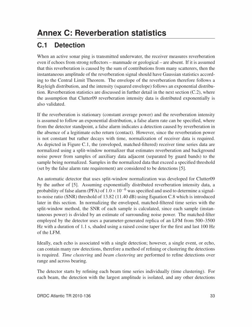
Figure C.1: Split-window normalizer. . . . . . . . . . . . . . . . . . . . . . . . . . 34

Figure C.2: Noise signal, g[n], shown in (a) generated by randomly sampling the

Gaussian pdf shown as the dashed line in (b). The pmf of the generated

signal is also shown in (b). . . . . . . . . . . . . . . . . . . . . . . . . . 38

Figure C.3: Enveloped noise signal, |ga[n]|, shown in (a) and its pmf in (b). The

theoretical Rayleigh pdf is also shown in (b). . . . . . . . . . . . . . . . 38

Figure C.4: Squared noise envelope signal (intensity), |ga[n]|2, shown in (a) and its

pmf in (b). The theoretical exponential pdf is also shown in (b). . . . . . 39

Figure C.5: Squared noise envelope signal (intensity) normalized with the

split-window normalizer shown in (a) and its pmf in (b). The

theoretical standard exponential pdf is also shown in (b). . . . . . . . . . 39

Figure C.6: Matched-filtered time series data for a single beam recorded during the

Clutter09 sea trial shown in (a), and its pmf in (b). The theoretical

Gaussian pdf is also shown in (b). . . . . . . . . . . . . . . . . . . . . . 41

Figure C.7: Samples 100 000–600 000 of the data shown in Figure C.6 are

displayed in (a), and its pmf in (b). The theoretical Gaussian pdf is also

shown in (b). . . . . . . . . . . . . . . . . . . . . . . . . . . . . . . . . 42

Figure C.8: Normalized intensity time series data for a single beam recorded during

the Clutter09 sea trial shown in (a), and its pmf in (b). The theoretical

standard exponential pdf is also shown in (b). . . . . . . . . . . . . . . . 43

Figure D.1: SNR calculation for an example echo. . . . . . . . . . . . . . . . . . . . 45

x DRDC Atlantic TR 2010-136

List of tables

Table 1: Identified echoes from Clutter07. . . . . . . . . . . . . . . . . . . . . . 17

Table 2: Features and principal components selected during training. . . . . . . . 18

Table 3: Identified echoes from Clutter09. . . . . . . . . . . . . . . . . . . . . . 21

Table A.1: Ship track waypoints during experiment in Clutter07. . . . . . . . . . . . 29

Table A.2: Ship track waypoints during experiment in Clutter09. . . . . . . . . . . . 29

Table B.1: Experimental details for Clutter07 and Clutter09. . . . . . . . . . . . . . 31

Table E.1: List of features ordered by discriminant score and overlap fraction

ranking methods. . . . . . . . . . . . . . . . . . . . . . . . . . . . . . . 47

DRDC Atlantic TR 2010-136 xi


xii DRDC Atlantic TR 2010-136

1 Introduction

Active sonar systems are used to detect underwater manmade objects of interest (targets)

that are too quiet to be reliably detected with passive sonar. In shallow coastal waters, active

sonar performance is degraded by false alarms caused by echoes returned from geological

seabed structures (clutter). To reduce false alarms, a method of distinguishing target echoes

from clutter echoes is required.

Sonar operators are capable of distinguishing targets from clutter by listening to their

echoes, and acheived high classification performance in a human listening experiment at

DRDC [1]. Following the experiment, DRDC developed an automatic aural classifer to

mimic the human listening process in order to automate this capability of sonar opera-

tors [2]. The classifier uses aural features – perceptual features derived from timbre – to

describe the echoes, and looks for trends in the features that allow the target echoes to be

separated from clutter.

Echo signals are affected by unstable environmental factors such as background noise and

sound propagation conditions. Because these factors are temporally variable, they can

cause differences in (otherwise identical) echoes received from pings sent out at different

times. Therefore, the aural features that describe the echoes must be temporally robust

– insensitive to changes in echoes from varying conditions – in order to train the aural

classifier in advance and then successfully classify echoes received after a lapse of time.

To investigate temporal robustness, an active sonar experiment was performed on the Malta

Plateau during a sea trial that took place in 2007 (Clutter07), and was repeated during a sea

trial in 2009 (Clutter09). The aural classifier is trained using target and clutter echoes

from the Clutter07 sea trial and then tested by performing classification on echoes from

the Clutter09 sea trial. The active sonar experiments performed during the sea trials were

very similar. In both experiments, a research ship followed the same route and transmitted

linear frequency modulated (LFM) pings. Using a towed array, echoes from each ping

were received from clutter, as well as from two manmade objects in the area which were

used as targets: the oil rig and the wellhead belonging to Campo Vega Oilfield. Over

95,000 echoes were collected, forming a database nearly two orders of magnitude larger

than databases used in previous studes [2, 3]. Although the experiments were conducted

in the same location, they were separated by two years, and the environmental conditions

were considerably different. This provides an excellent dataset with which to evaluate the

temporal robustness of the classifier.

In Section 2, details of the Clutter07 and Clutter09 experiments are reviewed and differ-

ences highlighted. Section 3 details the processing of data collected during the two experi-

ments in order to extract target and clutter echoes. A brief background on the aural classifier

is provided in Section 4. Section 5 presents the classification results, and conclusions are

highlighted in Section 6.

DRDC Atlantic TR 2010-136 1

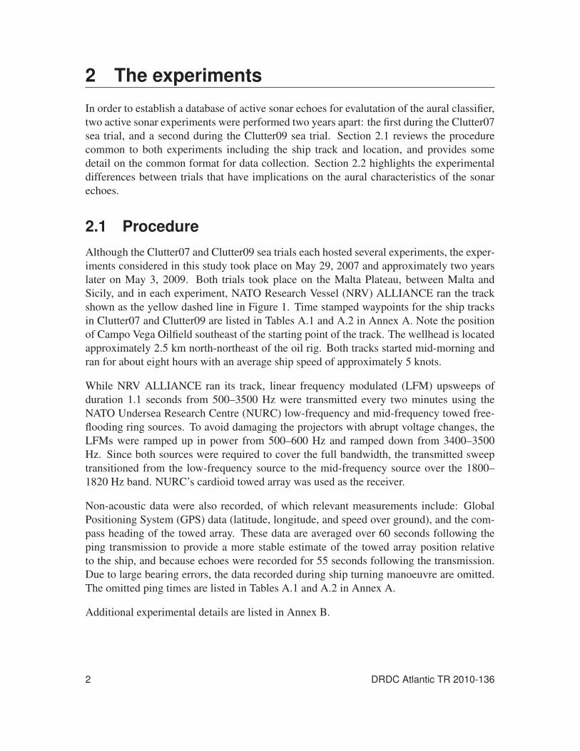
2 The experiments

In order to establish a database of active sonar echoes for evalutation of the aural classifier,

two active sonar experiments were performed two years apart: the first during the Clutter07

sea trial, and a second during the Clutter09 sea trial. Section 2.1 reviews the procedure

common to both experiments including the ship track and location, and provides some

detail on the common format for data collection. Section 2.2 highlights the experimental

differences between trials that have implications on the aural characteristics of the sonar

echoes.

2.1 ProcedureAlthough the Clutter07 and Clutter09 sea trials each hosted several experiments, the exper-

iments considered in this study took place on May 29, 2007 and approximately two years

later on May 3, 2009. Both trials took place on the Malta Plateau, between Malta and

Sicily, and in each experiment, NATO Research Vessel (NRV) ALLIANCE ran the track

shown as the yellow dashed line in Figure 1. Time stamped waypoints for the ship tracks

in Clutter07 and Clutter09 are listed in Tables A.1 and A.2 in Annex A. Note the position

of Campo Vega Oilfield southeast of the starting point of the track. The wellhead is located

approximately 2.5 km north-northeast of the oil rig. Both tracks started mid-morning and

ran for about eight hours with an average ship speed of approximately 5 knots.

While NRV ALLIANCE ran its track, linear frequency modulated (LFM) upsweeps of

duration 1.1 seconds from 500–3500 Hz were transmitted every two minutes using the

NATO Undersea Research Centre (NURC) low-frequency and mid-frequency towed free-

flooding ring sources. To avoid damaging the projectors with abrupt voltage changes, the

LFMs were ramped up in power from 500–600 Hz and ramped down from 3400–3500

Hz. Since both sources were required to cover the full bandwidth, the transmitted sweep

transitioned from the low-frequency source to the mid-frequency source over the 1800–

1820 Hz band. NURC’s cardioid towed array was used as the receiver.

Non-acoustic data were also recorded, of which relevant measurements include: Global

Positioning System (GPS) data (latitude, longitude, and speed over ground), and the com-

pass heading of the towed array. These data are averaged over 60 seconds following the

ping transmission to provide a more stable estimate of the towed array position relative

to the ship, and because echoes were recorded for 55 seconds following the transmission.

Due to large bearing errors, the data recorded during ship turning manoeuvre are omitted.

The omitted ping times are listed in Tables A.1 and A.2 in Annex A.

Additional experimental details are listed in Annex B.

2 DRDC Atlantic TR 2010-136

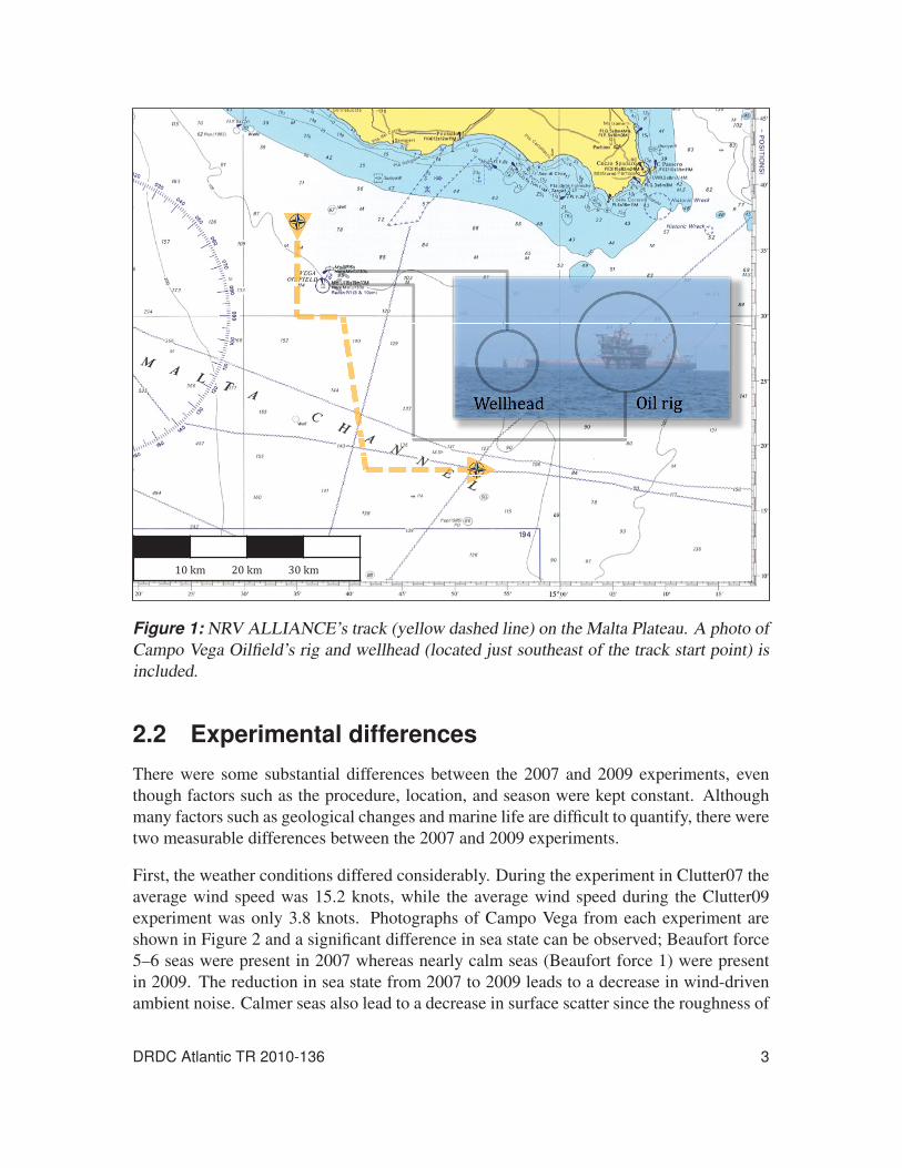
Figure 1: NRV ALLIANCE’s track (yellow dashed line) on the Malta Plateau. A photo of

Campo Vega Oilfield’s rig and wellhead (located just southeast of the track start point) is

included.

2.2 Experimental differencesThere were some substantial differences between the 2007 and 2009 experiments, even

though factors such as the procedure, location, and season were kept constant. Although

many factors such as geological changes and marine life are difficult to quantify, there were

two measurable differences between the 2007 and 2009 experiments.

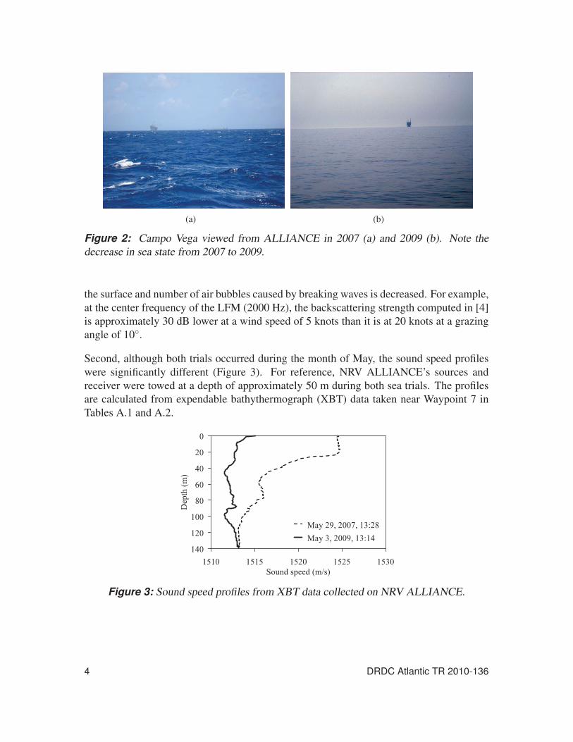
First, the weather conditions differed considerably. During the experiment in Clutter07 the

average wind speed was 15.2 knots, while the average wind speed during the Clutter09

experiment was only 3.8 knots. Photographs of Campo Vega from each experiment are

shown in Figure 2 and a significant difference in sea state can be observed; Beaufort force

5–6 seas were present in 2007 whereas nearly calm seas (Beaufort force 1) were present

in 2009. The reduction in sea state from 2007 to 2009 leads to a decrease in wind-driven

ambient noise. Calmer seas also lead to a decrease in surface scatter since the roughness of


(a) (b)

Figure 2: Campo Vega viewed from ALLIANCE in 2007 (a) and 2009 (b). Note the

decrease in sea state from 2007 to 2009.

the surface and number of air bubbles caused by breaking waves is decreased. For example,

at the center frequency of the LFM (2000 Hz), the backscattering strength computed in [4]

is approximately 30 dB lower at a wind speed of 5 knots than it is at 20 knots at a grazing

angle of 10◦.

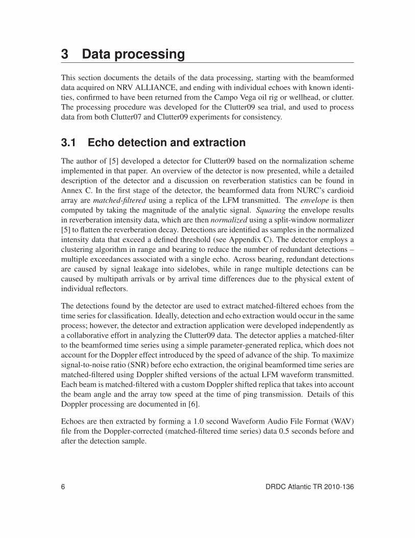
Second, although both trials occurred during the month of May, the sound speed profiles

were significantly different (Figure 3). For reference, NRV ALLIANCE’s sources and

receiver were towed at a depth of approximately 50 m during both sea trials. The profiles

are calculated from expendable bathythermograph (XBT) data taken near Waypoint 7 in

Tables A.1 and A.2.

Figure 3: Sound speed profiles from XBT data collected on NRV ALLIANCE.


While the 2007 sound speed profile is downward refracting, the 2009 profile is nearly

isospeed. The differences in the sound speed profiles and surface reflections contribute

to different sound propagation conditions for each trial; these could alter received echo

signals and the aural features that describe them.


3 Data processing

This section documents the details of the data processing, starting with the beamformed

data acquired on NRV ALLIANCE, and ending with individual echoes with known identi-

ties, confirmed to have been returned from the Campo Vega oil rig or wellhead, or clutter.

The processing procedure was developed for the Clutter09 sea trial, and used to process

data from both Clutter07 and Clutter09 experiments for consistency.

3.1 Echo detection and extractionThe author of [5] developed a detector for Clutter09 based on the normalization scheme

implemented in that paper. An overview of the detector is now presented, while a detailed

description of the detector and a discussion on reverberation statistics can be found in

Annex C. In the first stage of the detector, the beamformed data from NURC’s cardioid

array are matched-filtered using a replica of the LFM transmitted. The envelope is then

computed by taking the magnitude of the analytic signal. Squaring the envelope results

in reverberation intensity data, which are then normalized using a split-window normalizer

[5] to flatten the reverberation decay. Detections are identified as samples in the normalized

intensity data that exceed a defined threshold (see Appendix C). The detector employs a

clustering algorithm in range and bearing to reduce the number of redundant detections –

multiple exceedances associated with a single echo. Across bearing, redundant detections

are caused by signal leakage into sidelobes, while in range multiple detections can be

caused by multipath arrivals or by arrival time differences due to the physical extent of

individual reflectors.

The detections found by the detector are used to extract matched-filtered echoes from the

time series for classification. Ideally, detection and echo extraction would occur in the same

process; however, the detector and extraction application were developed independently as

a collaborative effort in analyzing the Clutter09 data. The detector applies a matched-filter

to the beamformed time series using a simple parameter-generated replica, which does not

account for the Doppler effect introduced by the speed of advance of the ship. To maximize

signal-to-noise ratio (SNR) before echo extraction, the original beamformed time series are

matched-filtered using Doppler shifted versions of the actual LFM waveform transmitted.

Each beam is matched-filtered with a custom Doppler shifted replica that takes into account

the beam angle and the array tow speed at the time of ping transmission. Details of this

Doppler processing are documented in [6].

Echoes are then extracted by forming a 1.0 second Waveform Audio File Format (WAV)

file from the Doppler-corrected (matched-filtered time series) data 0.5 seconds before and

after the detection sample.


3.2 Echo identificationIn order to have useful data for training and testing the classifier, each extracted echo needs

to be labelled as being returned from the oil rig, wellhead, or clutter1. Due to the large num-

ber of echoes, most of this process has been automated; however, some manual refining, as

explained in Section 3.2.2, is done to verify the automatic labelling.

3.2.1 Automated identification procedure

The contact location associated with each echo is determined from the range (time delay)

and the bearing angle (beam number) of the detection. The bearing uncertainty is the

largest contributor to the contact location error, since the beam width is as high as 14.8◦at the end-fire beam angle. Bearing accuracy could be improved by interpolating between

beams using the beam pattern, but this has not been implementeds

The coordinates of the oil rig and wellhead (targets) are known (see Appendix B), but

due to the sonar’s range and bearing resolution, and to ensure that no target echoes were

missed, all contacts within 2.4 km of each target position are considered as candidates for

association with that target. This distance corresponds to the separation between the oil

rig and wellhead. All other echoes are considered to be clutter. Additional precautions

were taken in order to ensure the oil rig and wellhead contact labels were not reversed: if a

contact was within range of both the oil rig and wellhead, the contact was assigned to the

closer object.

The large distance threshold resulted in many clutter echoes being associated with each of

the targets, which necessitated manual refining of the labels following the process described

in the next section.

3.2.2 Manual identification refining

Each ping produces at most one valid echo from each of the targets; however, the automatic

identification process can assign many contacts to a target for single ping, and these misla-

belled echoes must be corrected manually. This is accomplished by listening to the echoes

to make sure they sound similar to echoes already designated with the same label. To avoid

relying only on the listening test with its human factor uncertainty, each echo’s SNR, time

delay, and beam number are also considered. For each of the targets’ echoes, the values

for SNR, time delay, and beam number varied predictably over consecutive pings since the

ship travelled at a constant speed. Echoes with large discrepancies in the values expected

from the previous ping(s) could be quickly identified as clutter.

1Although not considered in this study, echoes from a passive acoustic target deployed in both experiments

also need to be identified so they can be isolated from the dataset.


The manual refining process ensured that the wellhead and oil rig had, at most, one echo,

and there was a high degree of confidence that it was correctly labelled. The process also

made sure that all of the echoes from the wellhead and oil rig were accounted for, and not

mislabelled as clutter. Pings with missing target echoes that were expected to be present

based on high SNRs observed in time-adjacent pings were investigated and recovered from

mislabelled clutter echoes in some cases.

3.3 Database expansion with off-beam target echoesThe database containing echoes with known identities is highly valuable; however, it can be

further improved to address two limitations. First, the number of clutter echoes extracted

is much greater than the number of target echoes. This is typical for active sonar; how-

ever, unbiased classification testing requires an equal number of target and clutter echoes.

Second, the SNR of the target echoes is typically greater than that of the clutter echoes for

the Clutter07 and Clutter09 data. To avoid classification biasing, they should have similar

SNR. In Section 5.1, the number of target and clutter echoes is made equal, and the SNR

distributions are matched, so that classification is not biased by prior probabilities (relative

number of clutter and target echoes) or by SNR.

There are a number of ways to accomplish matching the target and clutter population sizes

and SNRs. The number of clutter echoes could be limited to a relatively small number

of high SNR examples to match the population of target echoes. This would discard the

majority of the clutter data, and would not test the classifer on low SNR echoes – an

important aspect of its performance. A better solution is to obtain a large number of lower

SNR target echoes by selecting off-beam instances of echoes from sidelobe leakage that

were initially removed by the beam clustering of the detector. This technique was used

in [3], and in the present application it increases the number of target echoes by two orders

of magnitude, while at the same time obtaining a broader SNR distribution.

There is one technical detail that should be noted regarding this technique: particular at-

tention must be paid to the Doppler effect when extracting off-beam echoes. Recall that

the matched-filter used in the echo extraction process correlates each beam with a custom

Doppler-shifted replica that takes into account the ship’s radial velocity on that beam1. Off-

beam echoes are caused by leakage from the main beam signal, and although they may be

measured on a number of beams, they have propagated to the receiver from a single bear-

ing. Therefore, in extracting off-beam echoes, every beam is corrected for Doppler using

the same Doppler shift measured on the main beam, rather than using a different replica

for each beam as in the initial processing. This ensures that echo features are not affected

by improper Doppler correction, which is important for aural classification.

1The radial velocity is the rate of change of the distance between the ship and the contacts on a particular

beam and is calculated using the beam angle. For example, the magnitude of the radial velocity is equal to

the ship speed on end-fire beams, and is zero on broadside beams.


4 Aural classifier

The aural classifier mimics the human auditory system by conditioning signals (i.e., active

sonar echoes) in a similar way as the outer and inner human ear, and by simulating the cog-

nitive process through representing the echoes as perceptual features. A Gaussian classifier

that uses Bayes decision theory then simulates the human decision-making process, in this

case to determine whether an echo should be designated as a target or as clutter. A brief

overview of the aural feature calculation is given in Section 4.1, while a full description

of the specific features is detailed in [3]. Methods for reducing the feature dimensionality

are considered in Section 4.2 to address the problems assosicated with limited numbers

of samples. The generic Gaussian classifier is reviewed in Section 4.3, and metrics for

evaluating its performance are presented in Section 4.4.

4.1 Aural feature calculationThe human auditory system mimiced by the aural classifier can be separated into 2 pro-

cesses: the mechanical process that conditions signals incident on the ear, and the cog-

nitive process in which the brain perceives the nerve signals generated from the incident

mechanical signals.

The first stage of the auditory system is mimiced by processing echoes with a model of

the mechanical response of the human ear. An auditory filter bank produces approximately

50 bandpass-filtered versions of the original echo, representing the narrow-band responses

at locations along the cochlea (inner ear) that are excited at different frequencies. In the

human ear, the basilar membrane converts these mechanical responses into nerve signals

which are used by the cognitive process.

The cognitive process is extremely complex and cannot be captured in a model. In order to

account for this process and create a perceptual representation of each echo, the classifier

extracts features derived from timbre which is used to describe perceptual features in the

field of musical acoustics. These perceptual-based quantities (i.e., attack time, duration,

loudness, etc.) are calculated for all of the bandpass-filtered versions of each echo, and

summary statistics including the minimum, maximum, and mean, are used to produce 58

aural features. The reader is referred to [3] for a detailed description of the aural features.

Some features may be redundant if they are highly correlated over the echoes in a particular

dataset under evaluation. In other words, if a feature value is known for a given echo, and

the value of a different feature can be simply calculated from the first feature value, then one

of the features is redundant. Redundant features do not provide additional information on

the echoes and are therefore removed from consideration. There are typically less than 20

redundant features for datasets of echoes from the Clutter07 and Clutter09 databases. This

leaves over 30 non-redundant features that are reduced to a smaller number of dimensions


in the next section in order to permit their implementation in a practical manner.

4.2 Feature dimension reduction4.2.1 Curse of dimensionality

The aural classifier assumes that the aural feature values are Gaussian distributed, and this

will be discussed further in Section 4.3. A sample population from any statistical distri-

bution requires adequate spatial density of samples in order to accurately represent the

distribution. As the dimensionality of each sample increases, the number of samples must

increase exponentially to maintain a constant sampling density. This is known as the curseof dimensionality. If N is the number of samples required for a dense population in a single

dimension, N p is the sample size required to maintain a dense population in p dimen-

sions [7]. For simplicity, imagine that a Gaussian distribution can be densely represented

by only 10 samples in one dimension. In order to maintain population density in 58 di-

mensions (the number of features used by the classifier), the sample size needs to be 1058,

which is impractical. Clearly one must reduce the feature dimensionality. Sample sizes

encountered in this study are relatively large, but do not exceed the order of 10,000 echoes.

Even if 10 samples were adequate in a single dimension, the number of dimensions should

not exceed 4, since 104 = 10,000. Feature selection and principal component analysis are

techniques used to reduce dimensionality, and although the (optimistic) maximum number

of 4 dimensions is not taken to be a restriction in this work, it should be kept in mind.

4.2.2 Feature selection

Currently, the aural classifier reduces the number of non-redundant features by individually

ranking them based on how well they can discriminate between targets and clutter in the

training dataset. The number of features kept is user defined and is typically less than 15.

There are various methods of ranking features, and two are considered in this study: the

overlap fraction of class probability density functions, and discriminant score.

4.2.2.1 Overlap fraction

For a given feature, the overlap fraction method calculates the mean and variance of each

class over the entire training dataset. Using these parameters, a Gaussian probability den-

sity function (pdf) is constructed for each class, and the fraction of the total area under the

pdfs common to all of the classes is calculated. Intuitively, low overlap fractions indicate

features with separation between classes. One potential downside of this method is that it

allows features with identical means to achieve high ranking if they have large differences

in their variances, as depicted in Figure 4. Although discrimination by variance alone is

not unreasonable, explicitly including separation of means in the ranking metric is more

intuitive, and this is the approach is taken in discriminant analysis.


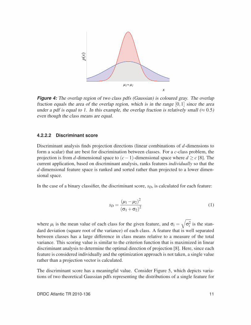
Figure 4: The overlap region of two class pdfs (Gaussian) is coloured gray. The overlap

fraction equals the area of the overlap region, which is in the range [0,1] since the area

under a pdf is equal to 1. In this example, the overlap fraction is relatively small (≈ 0.5)

even though the class means are equal.

4.2.2.2 Discriminant score

Discriminant analysis finds projection directions (linear combinations of d-dimensions to

form a scalar) that are best for discrimination between classes. For a c-class problem, the

projection is from d-dimensional space to (c−1)-dimensional space where d ≥ c [8]. The

current application, based on discriminant analysis, ranks features individually so that the

d-dimensional feature space is ranked and sorted rather than projected to a lower dimen-

sional space.

In the case of a binary classifier, the discriminant score, sD, is calculated for each feature:

sD =(μ1 −μ2)

2

(σ1 +σ2)2

(1)

where μi is the mean value of each class for the given feature, and σi =√

σ2i is the stan-

dard deviation (square root of the variance) of each class. A feature that is well separated

between classes has a large difference in class means relative to a measure of the total

variance. This scoring value is similar to the criterion function that is maximized in linear

discriminant analysis to determine the optimal direction of projection [8]. Here, since each

feature is considered individually and the optimization approach is not taken, a single value

rather than a projection vector is calculated.

The discriminant score has a meaningful value. Consider Figure 5, which depicts varia-

tions of two theoretical Gaussian pdfs representing the distributions of a single feature for


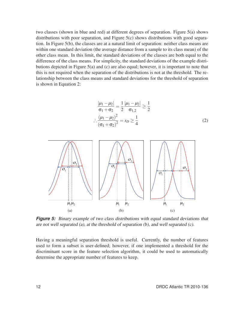
two classes (shown in blue and red) at different degrees of separation. Figure 5(a) shows

distributions with poor separation, and Figure 5(c) shows distributions with good separa-

tion. In Figure 5(b), the classes are at a natural limit of separation: neither class means are

within one standard deviation (the average distance from a sample to its class mean) of the

other class mean. In this limit, the standard deviations of the classes are both equal to the

difference of the class means. For simplicity, the standard deviations of the example distri-

butions depicted in Figure 5(a) and (c) are also equal; however, it is important to note that

this is not required when the separation of the distributions is not at the threshold. The re-

lationship between the class means and standard deviations for the threshold of separation

is shown in Equation 2:

|μ1 −μ2|σ1 +σ2

=1

2

|μ1 −μ2|σ1,2

≥ 1

2

∴ (μ1 −μ2)2

(σ1 +σ2)2= sD ≥ 1

4(2)

(a) (b) (c)

Figure 5: Binary example of two class distributions with equal standard deviations that

are not well separated (a), at the threshold of separation (b), and well separated (c).

Having a meaningful separation threshold is useful. Currently, the number of features

used to form a subset is user-defined; however, if one implemented a threshold for the

discriminant score in the feature selection algorithm, it could be used to automatically

determine the appropriate number of features to keep.


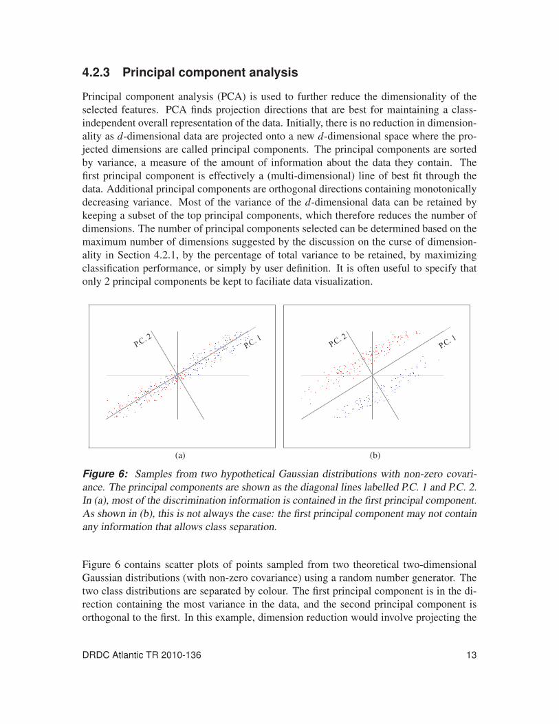
4.2.3 Principal component analysis

Principal component analysis (PCA) is used to further reduce the dimensionality of the

selected features. PCA finds projection directions that are best for maintaining a class-

independent overall representation of the data. Initially, there is no reduction in dimension-

ality as d-dimensional data are projected onto a new d-dimensional space where the pro-

jected dimensions are called principal components. The principal components are sorted

by variance, a measure of the amount of information about the data they contain. The

first principal component is effectively a (multi-dimensional) line of best fit through the

data. Additional principal components are orthogonal directions containing monotonically

decreasing variance. Most of the variance of the d-dimensional data can be retained by

keeping a subset of the top principal components, which therefore reduces the number of

dimensions. The number of principal components selected can be determined based on the

maximum number of dimensions suggested by the discussion on the curse of dimension-

ality in Section 4.2.1, by the percentage of total variance to be retained, by maximizing

classification performance, or simply by user definition. It is often useful to specify that

only 2 principal components be kept to faciliate data visualization.

(a) (b)

Figure 6: Samples from two hypothetical Gaussian distributions with non-zero covari-

ance. The principal components are shown as the diagonal lines labelled P.C. 1 and P.C. 2.

In (a), most of the discrimination information is contained in the first principal component.

As shown in (b), this is not always the case: the first principal component may not contain

any information that allows class separation.

Figure 6 contains scatter plots of points sampled from two theoretical two-dimensional

Gaussian distributions (with non-zero covariance) using a random number generator. The

two class distributions are separated by colour. The first principal component is in the di-

rection containing the most variance in the data, and the second principal component is

orthogonal to the first. In this example, dimension reduction would involve projecting the


data onto the first principal component axis and discarding the second principal compo-

nent. It should be noted that PCA does not take class information into consideration. This

is demonstrated in Figure 6(b) where the second principal component, the only one that

allows class discrimination, would be discarded because it contains less overall variance

than the first principal component.

4.3 Gaussian-based classifierAfter the aural features are calculated and reduced with feature selection and PCA, a

Gaussian-based classifier is applied in which a Gaussian pdf is fit to each class in the

training dataset. Although the distributions of the features, and therefore the principal com-

ponents, are assumed to follow a Gaussian distribution as in [3], this is not typically tested

for each dataset, and it is accepted that even if the data do not strictly follow a Gaussian

distribution, a simple, successful classification decision boundary can be computed.

The default operating point of the classifier is chosen according to Bayesian decision the-

ory and corresponds to the Bayes rate [7] or minimum-error-rate [8]. At this operating

point, echoes are classified to the more probable class – the class with the higher poste-

rior probability. The posterior probabilities are represented by P(T | x) and P(C | x) for

the clutter and target classes, respectively, and represent the probability of an echo coming

from the target class, T , and the probability of an echo coming from the clutter class, C,

given the measurement, x. In the case of equal prior probabilities (equal number of samples

in class), the decision boundary formed by this operating point is simply the intersection

of the Gaussian pdfs. If the prior probabilities are unequal, the posterior probabilities are

weighted, and the decision boundary biases classification toward the class with the larger

sample size.

The posterior probabilities for the target and clutter classes are calculated from the target

and clutter pdfs, p(x | T ) and p(x |C), using Equations 5 and 3:

P(T | x) =P(T ) · p(x | T )

P(C) · p(x |C)+P(T ) · p(x | T )(3)

P(C | x) =P(C) · p(x |C)

P(C) · p(x |C)+P(T ) · p(x | T )(4)

where P(T ) and P(C) are the prior probabilities of the target and clutter classes, and the

common denominator normalizes the posterior probabilities such that:

P(T | x)+P(C | x) = 1 (5)


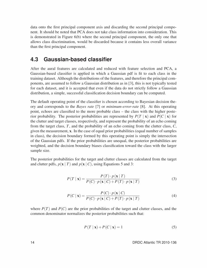
Figures 7(b) and (d) show the top views of the surfaces for visualization of the decision

boundaries. In this case of equal prior probabilities (same number of target and clutter

echoes), the decision regions in (b) and (d) are identical, although they may appear slightly

different due to the visualization view points.

(a) (b)

(c) (d)

Figure 7: Hypothetical clutter (blue) and target (red) pdfs shown in (a) and (b), and cor-

responding posterior probabilities shown in (c) and (d).


4.4 Classification performance metricsThe simplest measure of performance is classification accuracy, which is defined as the

percentage of echoes correctly classified. Individual class accuracies should be calculated,

since this information is lost in a total accuracy value. In the multi-class case, accuracy

is the only performance metric available; however, in the binary-class case presented in

this paper, the receiver-operating-characteristic (ROC) curve, which plots probability of

detection versus probability of false alarm, provides more insight on classifier performance.

The default minimum-error-rate operating point specified in Section 4.3 was chosen ac-

cording to Bayes decision theory, and depending on the relative cost of misclassifying

targets and clutter for a given application, this operating point may not be preferred. ROC

curves provide a means of quickly evaluating how the classifier is performing at all oper-

ating points.

A scalar measure of this overall performance is obtained by integrating the area under the

ROC curve, AROC. The ideal ROC curve has a probability of detection of 1 at all false alarm

rates (from 0–1), so AROC = 1 for perfect classification. Theoretically, if classification is

performed by random guessing, AROC = 0.5. AROC > 0.9 was considered to indicate very

successful performance in previous studies on classification of active sonar echoes [2], and

this convention is adopted here.


5 Classification results

Recall that the temporal robustness of the aural classifier will be evaluated by training the

classifier using data from Clutter07 and testing the classifier using data from Clutter09.

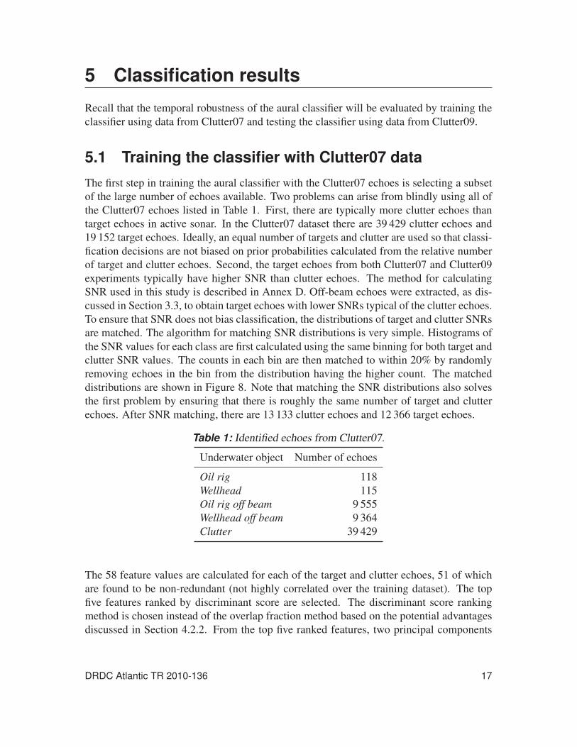
5.1 Training the classifier with Clutter07 dataThe first step in training the aural classifier with the Clutter07 echoes is selecting a subset

of the large number of echoes available. Two problems can arise from blindly using all of

the Clutter07 echoes listed in Table 1. First, there are typically more clutter echoes than

target echoes in active sonar. In the Clutter07 dataset there are 39 429 clutter echoes and

19 152 target echoes. Ideally, an equal number of targets and clutter are used so that classi-

fication decisions are not biased on prior probabilities calculated from the relative number

of target and clutter echoes. Second, the target echoes from both Clutter07 and Clutter09

experiments typically have higher SNR than clutter echoes. The method for calculating

SNR used in this study is described in Annex D. Off-beam echoes were extracted, as dis-

cussed in Section 3.3, to obtain target echoes with lower SNRs typical of the clutter echoes.

To ensure that SNR does not bias classification, the distributions of target and clutter SNRs

are matched. The algorithm for matching SNR distributions is very simple. Histograms of

the SNR values for each class are first calculated using the same binning for both target and

clutter SNR values. The counts in each bin are then matched to within 20% by randomly

removing echoes in the bin from the distribution having the higher count. The matched

distributions are shown in Figure 8. Note that matching the SNR distributions also solves

the first problem by ensuring that there is roughly the same number of target and clutter

echoes. After SNR matching, there are 13 133 clutter echoes and 12 366 target echoes.

Table 1: Identified echoes from Clutter07.

Underwater object Number of echoes

Oil rig 118

Wellhead 115

Oil rig off beam 9 555

Wellhead off beam 9 364

Clutter 39 429

The 58 feature values are calculated for each of the target and clutter echoes, 51 of which

are found to be non-redundant (not highly correlated over the training dataset). The top

five features ranked by discriminant score are selected. The discriminant score ranking

method is chosen instead of the overlap fraction method based on the potential advantages

discussed in Section 4.2.2. From the top five ranked features, two principal components


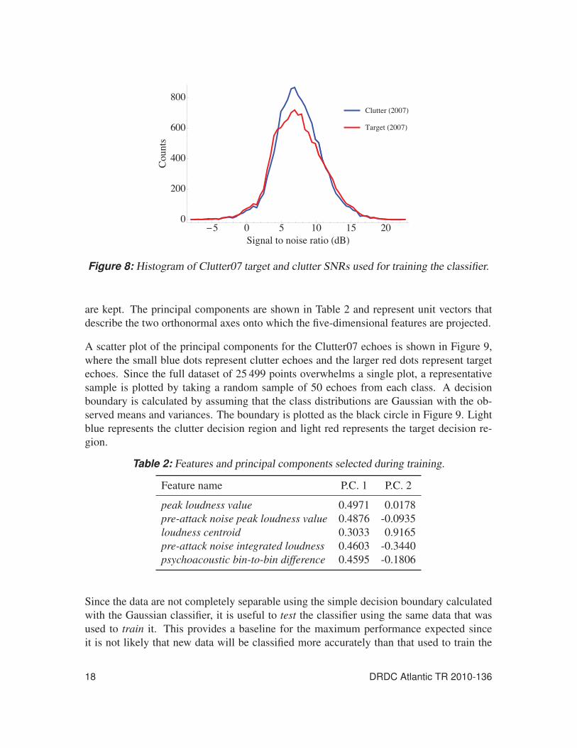
Figure 8: Histogram of Clutter07 target and clutter SNRs used for training the classifier.

are kept. The principal components are shown in Table 2 and represent unit vectors that

describe the two orthonormal axes onto which the five-dimensional features are projected.

A scatter plot of the principal components for the Clutter07 echoes is shown in Figure 9,

where the small blue dots represent clutter echoes and the larger red dots represent target

echoes. Since the full dataset of 25 499 points overwhelms a single plot, a representative

sample is plotted by taking a random sample of 50 echoes from each class. A decision

boundary is calculated by assuming that the class distributions are Gaussian with the ob-

served means and variances. The boundary is plotted as the black circle in Figure 9. Light

blue represents the clutter decision region and light red represents the target decision re-

gion.

Table 2: Features and principal components selected during training.

Feature name P.C. 1 P.C. 2

peak loudness value 0.4971 0.0178

pre-attack noise peak loudness value 0.4876 -0.0935

loudness centroid 0.3033 0.9165

pre-attack noise integrated loudness 0.4603 -0.3440

psychoacoustic bin-to-bin difference 0.4595 -0.1806

Since the data are not completely separable using the simple decision boundary calculated

with the Gaussian classifier, it is useful to test the classifier using the same data that was

used to train it. This provides a baseline for the maximum performance expected since

it is not likely that new data will be classified more accurately than that used to train the


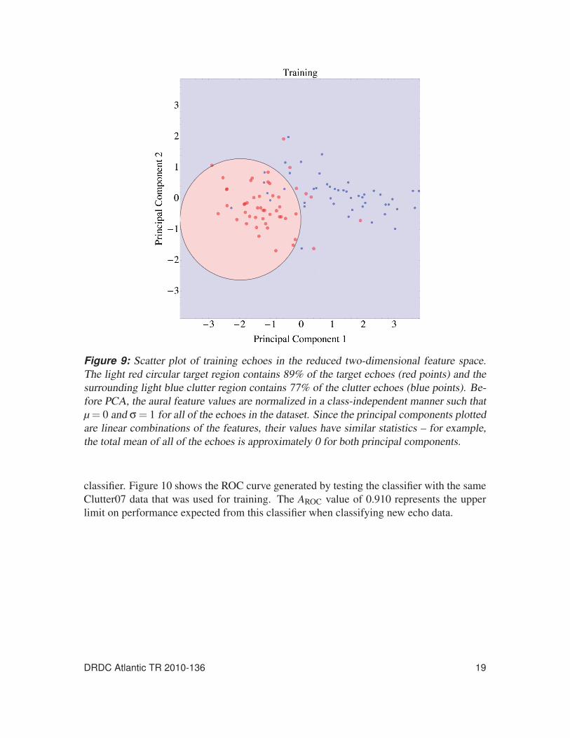
Figure 9: Scatter plot of training echoes in the reduced two-dimensional feature space.

The light red circular target region contains 89% of the target echoes (red points) and the

surrounding light blue clutter region contains 77% of the clutter echoes (blue points). Be-

fore PCA, the aural feature values are normalized in a class-independent manner such that

μ = 0 and σ = 1 for all of the echoes in the dataset. Since the principal components plotted

are linear combinations of the features, their values have similar statistics – for example,

the total mean of all of the echoes is approximately 0 for both principal components.

classifier. Figure 10 shows the ROC curve generated by testing the classifier with the same

Clutter07 data that was used for training. The AROC value of 0.910 represents the upper

limit on performance expected from this classifier when classifying new echo data.


Figure 10: ROC curve for the Clutter07 training set.

5.2 Testing the classifier with Clutter09 dataThe testing dataset has fewer limitations than the training set; after all, the purpose of a

classifier is to classify unidentified echoes. However, for this controlled test in which the

identities of the echoes are known, the procedure used on the training dataset to avoid

classification biasing is repeated for the testing dataset. In both training and testing phases,

it is important to have a similar number of target and clutter echoes when evaluating a

classifier using ROC curves. The performance indicated by a ROC curve can be over

optimistic when very few targets exist relative to the number of clutter echoes [9], which is

typically the case in active sonar.

The original Clutter09 dataset is described in Table 3. It is not necessary to match the target

and clutter SNR distributions, but this ensures an equal number of target and clutter echoes,

and even in the testing phase, the classification results should not be biased by differences

in SNR that may lead to higher discrimination between target and clutter echoes. To be

consistent with the training SNRs, the testing SNR distributions are made similar by bin-

matching each of the target and clutter SNR distributions to within 20% of their respective

training distributions. Since a 20% discrepancy was allowed between bins in the training

distributions, a maximum discrepancy of 44% (1.22 = 1.44) is possible between the testing

target and clutter SNR distributions. Allowing some discrepancy avoids discarding too


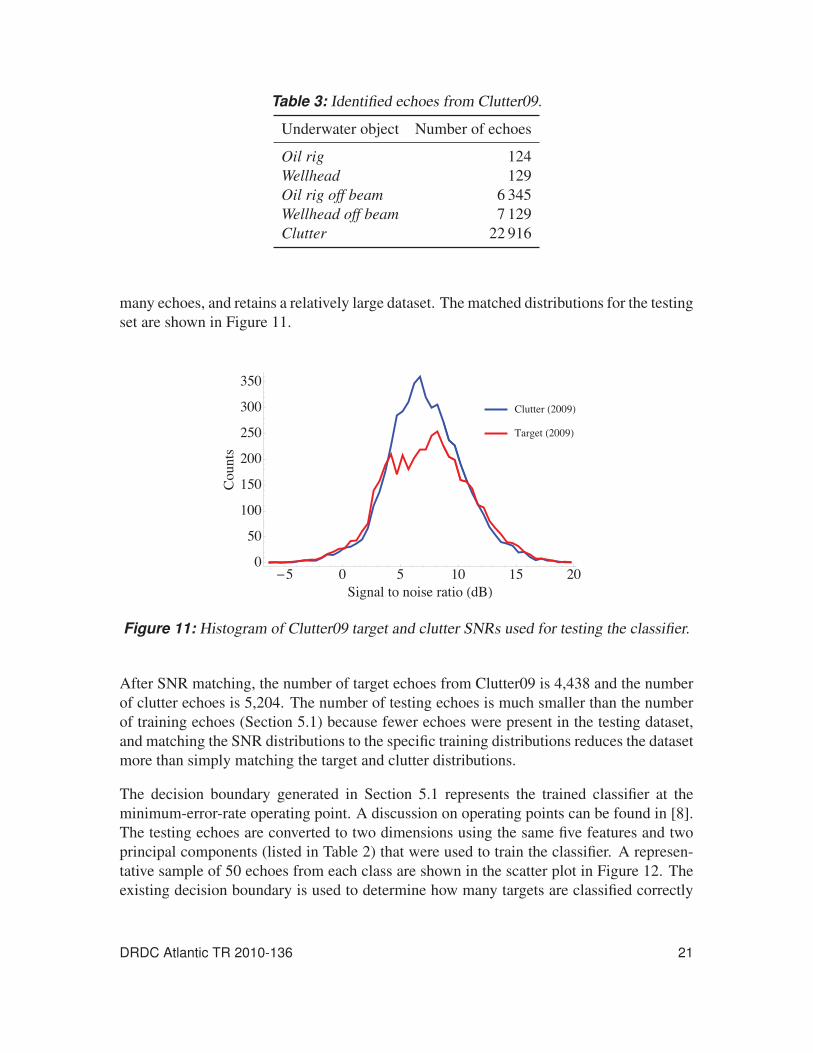
Table 3: Identified echoes from Clutter09.

Underwater object Number of echoes

Oil rig 124

Wellhead 129

Oil rig off beam 6 345

Wellhead off beam 7 129

Clutter 22 916

many echoes, and retains a relatively large dataset. The matched distributions for the testing

set are shown in Figure 11.

Figure 11: Histogram of Clutter09 target and clutter SNRs used for testing the classifier.

After SNR matching, the number of target echoes from Clutter09 is 4,438 and the number

of clutter echoes is 5,204. The number of testing echoes is much smaller than the number

of training echoes (Section 5.1) because fewer echoes were present in the testing dataset,

and matching the SNR distributions to the specific training distributions reduces the dataset

more than simply matching the target and clutter distributions.

The decision boundary generated in Section 5.1 represents the trained classifier at the

minimum-error-rate operating point. A discussion on operating points can be found in [8].

The testing echoes are converted to two dimensions using the same five features and two

principal components (listed in Table 2) that were used to train the classifier. A represen-

tative sample of 50 echoes from each class are shown in the scatter plot in Figure 12. The

existing decision boundary is used to determine how many targets are classified correctly


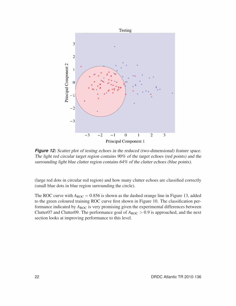
Figure 12: Scatter plot of testing echoes in the reduced (two-dimensional) feature space.

The light red circular target region contains 90% of the target echoes (red points) and the

surrounding light blue clutter region contains 64% of the clutter echoes (blue points).

(large red dots in circular red region) and how many clutter echoes are classified correctly

(small blue dots in blue region surrounding the circle).

The ROC curve with AROC = 0.856 is shown as the dashed orange line in Figure 13, added

to the green coloured training ROC curve first shown in Figure 10. The classification per-

formance indicated by AROC is very promising given the experimental differences between

Clutter07 and Clutter09. The performance goal of AROC > 0.9 is approached, and the next

section looks at improving performance to this level.


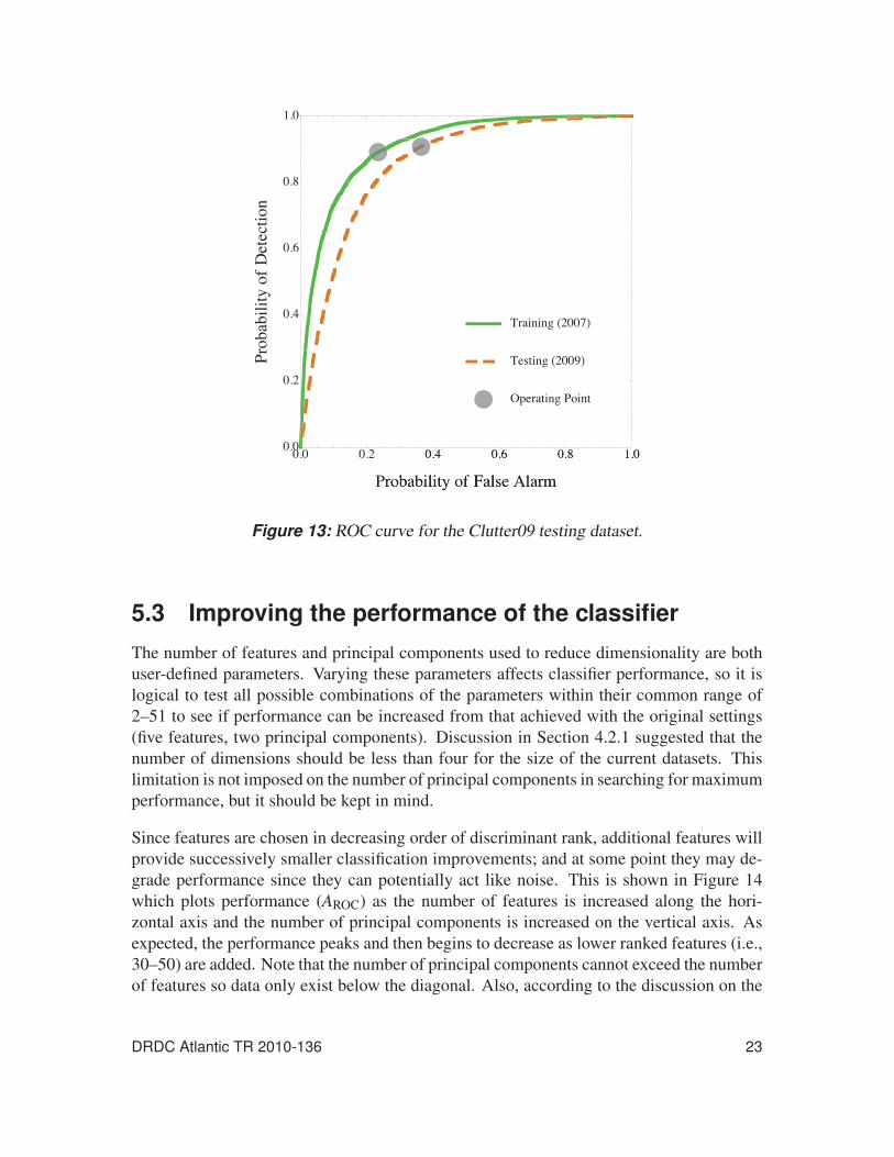
Figure 13: ROC curve for the Clutter09 testing dataset.

5.3 Improving the performance of the classifierThe number of features and principal components used to reduce dimensionality are both

user-defined parameters. Varying these parameters affects classifier performance, so it is

logical to test all possible combinations of the parameters within their common range of

2–51 to see if performance can be increased from that achieved with the original settings

(five features, two principal components). Discussion in Section 4.2.1 suggested that the

number of dimensions should be less than four for the size of the current datasets. This

limitation is not imposed on the number of principal components in searching for maximum

performance, but it should be kept in mind.

Since features are chosen in decreasing order of discriminant rank, additional features will

provide successively smaller classification improvements; and at some point they may de-

grade performance since they can potentially act like noise. This is shown in Figure 14

which plots performance (AROC) as the number of features is increased along the hori-

zontal axis and the number of principal components is increased on the vertical axis. As

expected, the performance peaks and then begins to decrease as lower ranked features (i.e.,

30–50) are added. Note that the number of principal components cannot exceed the number

of features so data only exist below the diagonal. Also, according to the discussion on the


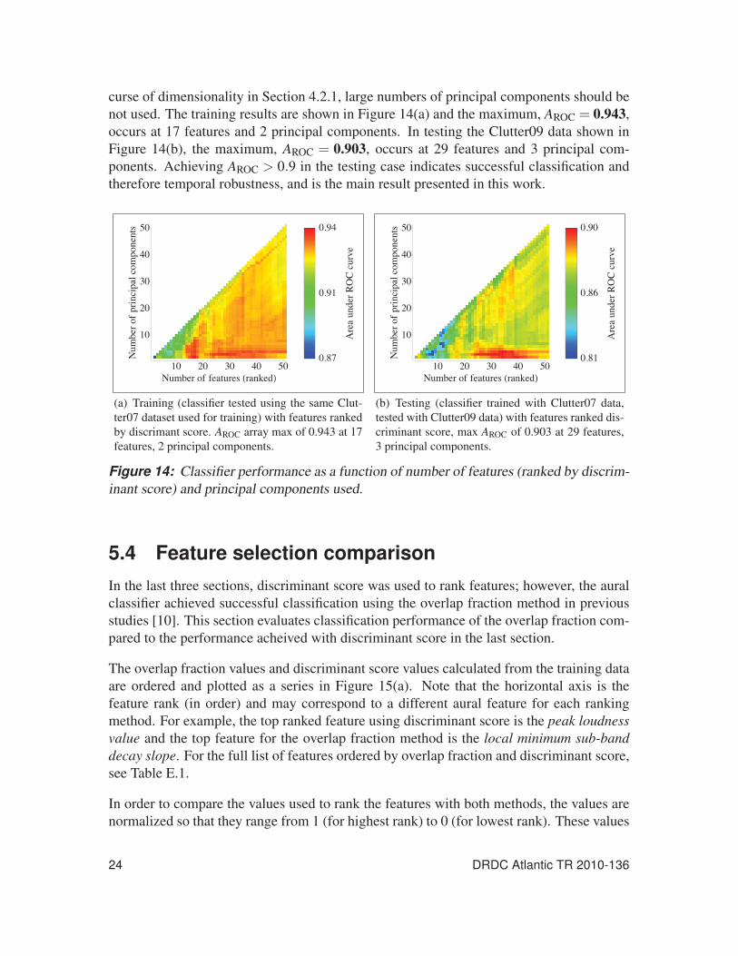
curse of dimensionality in Section 4.2.1, large numbers of principal components should be

not used. The training results are shown in Figure 14(a) and the maximum, AROC = 0.943,

occurs at 17 features and 2 principal components. In testing the Clutter09 data shown in

Figure 14(b), the maximum, AROC = 0.903, occurs at 29 features and 3 principal com-

ponents. Achieving AROC > 0.9 in the testing case indicates successful classification and

therefore temporal robustness, and is the main result presented in this work.

(a) Training (classifier tested using the same Clut-

ter07 dataset used for training) with features ranked

by discrimant score. AROC array max of 0.943 at 17

features, 2 principal components.

(b) Testing (classifier trained with Clutter07 data,

tested with Clutter09 data) with features ranked dis-

criminant score, max AROC of 0.903 at 29 features,

3 principal components.

Figure 14: Classifier performance as a function of number of features (ranked by discrim-

inant score) and principal components used.

5.4 Feature selection comparisonIn the last three sections, discriminant score was used to rank features; however, the aural

classifier achieved successful classification using the overlap fraction method in previous

studies [10]. This section evaluates classification performance of the overlap fraction com-

pared to the performance acheived with discriminant score in the last section.

The overlap fraction values and discriminant score values calculated from the training data

are ordered and plotted as a series in Figure 15(a). Note that the horizontal axis is the

feature rank (in order) and may correspond to a different aural feature for each ranking

method. For example, the top ranked feature using discriminant score is the peak loudnessvalue and the top feature for the overlap fraction method is the local minimum sub-banddecay slope. For the full list of features ordered by overlap fraction and discriminant score,

see Table E.1.

In order to compare the values used to rank the features with both methods, the values are

normalized so that they range from 1 (for highest rank) to 0 (for lowest rank). These values


(a) Discriminant scores (solid line) and

overlap fractions (dashed line) versus their

respective ordered features.

(b) Normalized discriminant scores (solid

line) and overlap fractions (dashed line)

decreasing with respective ordered feature

rank.

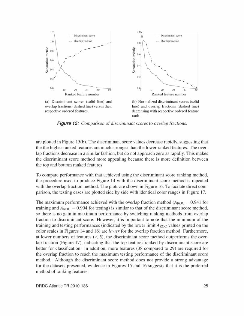
Figure 15: Comparison of discriminant scores to overlap fractions.

are plotted in Figure 15(b). The discriminant score values decrease rapidly, suggesting that

the the higher ranked features are much stronger than the lower ranked features. The over-

lap fractions decrease in a similar fashion, but do not approach zero as rapidly. This makes

the discriminant score method more appealing because there is more definition between

the top and bottom ranked features.

To compare performance with that achieved using the discriminant score ranking method,

the procedure used to produce Figure 14 with the discriminant score method is repeated

with the overlap fraction method. The plots are shown in Figure 16. To facilate direct com-

parison, the testing cases are plotted side by side with identical color ranges in Figure 17.

The maximum performance achieved with the overlap fraction method (AROC = 0.941 for

training and AROC = 0.904 for testing) is similar to that of the discriminant score method,

so there is no gain in maximum performance by switching ranking methods from overlap

fraction to discriminant score. However, it is important to note that the minimum of the

training and testing performances (indicated by the lower limit AROC values printed on the

color scales in Figures 14 and 16) are lower for the overlap fraction method. Furthermore,

at lower numbers of features (< 5), the discriminant score method outperforms the over-

lap fraction (Figure 17), indicating that the top features ranked by discriminant score are

better for classification. In addition, more features (38 compared to 29) are required for

the overlap fraction to reach the maximum testing performance of the discriminant score

method. Although the discriminant score method does not provide a strong advantage

for the datasets presented, evidence in Figures 15 and 16 suggests that it is the preferred

method of ranking features.


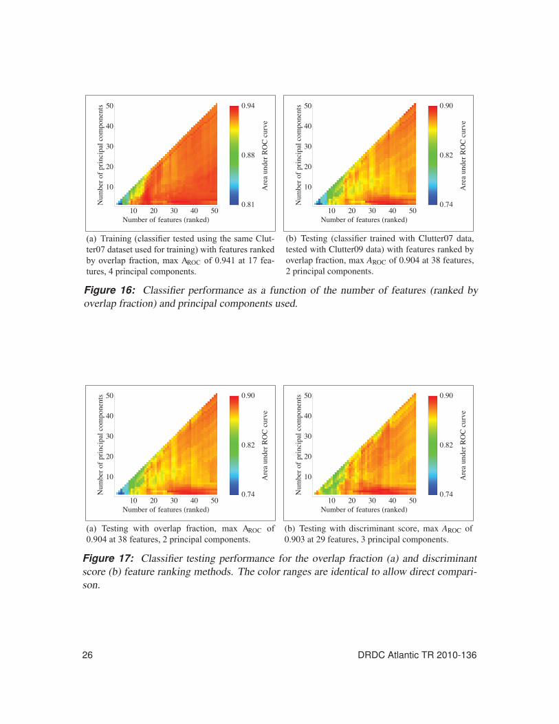
(a) Training (classi er tested using the same Clut-ter07 dataset used for training) with features rankedby overlap fraction, max AROC of 0.941 at 17 fea-tures, 4 principal components.

(a) Testing with overlap fraction, max AROC of0.904 at 38 features, 2 principal components.

(b) Testing with discriminant score, max AROC of

0.903 at 29 features, 3 principal components.

Figure 17: Classifier testing performance for the overlap fraction (a) and discriminant

score (b) feature ranking methods. The color ranges are identical to allow direct compari-

son.


(b) Testing (classifier trained with Clutter07 data,

tested with Clutter09 data) with features ranked by

overlap fraction, max AROC of 0.904 at 38 features,

2 principal components.

Figure 16: Classifier performance as a function of the number of features (ranked by

overlap fraction) and principal components used.

6 Conclusions and future work

This paper examined the temporal robustness of DRDC’s aural classifier. The aural classi-

fier mimics the human auditory system in order to automate the capability of sonar opera-

tors to distinguish clutter from targets. Binary classification of Clutter09 echoes as either

targets or clutter was performed after training the classifier with older data from a previ-

ous sea trial, Clutter07. Successful classification was indicated by achieving an area under

the ROC curve of AROC = 0.903, recalling that AROC = 1 for perfect classification and

AROC = 0.5 for random guessing. This is a very promising result in light of the different

sound propagation conditions between experiments.

The aural classifier has high potential for implementation in military active sonar systems,

since it can be trained in advance and used for long-term classification of echoes over a

range of environmental conditions. Operational sonar systems frequently mistake clutter

for targets in coastal waters, resulting in high false alarm rates. By providing false alarm re-

duction, the aural classifier could greatly improve detection performance of these systems,

and also reduce operator load.

Future work will involve expanding the database to include data from additional experi-

ments in Clutter09. The dependence of classification on SNR will also be examined to

study the difficult case of classifying low SNR echoes. Finally, true discriminant analysis

will be implemented and tested, which will accomplish dimension reduction by project-

ing the aural features onto axes that maximize discrimation between targets and clutter.

This will be compared to the feature selection method and principal component analysis

technique currently used to reduce dimensionality.


References

[1] Allen, N. (2008), Receiver-operating-characteristic (ROC) analysis applied to

listening-test data: Measures of performance in aural classification of sonar echoes,

(DRDC Atlantic TM 2007-353) Defence R&D Canada – Atlantic.

[2] Hines, P. C., Allen, N., and Young, V. W. (2008), Aural classification for active

sonar: Final Report for TIF Project 11CQ11 “Aural Discrimination of True Targets

from Geological Clutter”, (DRDC Atlantic TM 2007-361) Defence R&D Canada –

Atlantic.

[3] Young, V. W. and Hines, P. C. (2007), Perception-based automatic classification of

impulsive-source active sonar echoes, J. Acoust. Soc. Am., 122(3), 1502–1517.

[4] Urick, R. J. (1975), Principles of underwater sound, 2nd ed, McGraw-Hill, Inc.

[5] Abraham, D. A. and Willett, P. K. (2002), Active sonar detection in shallow water

using the Page test, IEEE Journal of Oceanic Engineering, 27(1), 35–46.

[6] Hood, J. and McInnis, J. (2010), Integrated tracker and aural classifier (ITAC)

development, (DRDC Atlantic CR 2010-049) Akoostix Inc.

[7] Hastie, T., Tibshirani, R., and Friedman, J. (2001), The elements of statistical

learning; data mining, inference, and prediction, New York: Springer.

[8] Duda, R. O., Hart, P. E., and Stork, D. G. (2001), Pattern Classification, 2nd ed,

Wiley-Interscience.

[9] Davis, J. and Goadrich, M. (2006), The relationship between precision-recall and

ROC curves, In Proceedings of the 23rd International Conference on MachineLearning, Pittsburgh, PA.

[10] Hines, P. C., Young, V. W., and Scrutton, J. (2008), Aural classification of

coherent-source active sonar echoes, In Proceedings: International Symposium onUnderwater Reverberation and Clutter, Lerici, Italy.


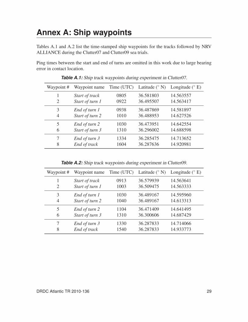
Annex A: Ship waypoints

Tables A.1 and A.2 list the time-stamped ship waypoints for the tracks followed by NRV

ALLIANCE during the Clutter07 and Clutter09 sea trials.

Ping times between the start and end of turns are omitted in this work due to large bearing

error in contact location.

Table A.1: Ship track waypoints during experiment in Clutter07.

Waypoint # Waypoint name Time (UTC) Latitude (◦ N) Longitude (◦ E)

1 Start of track 0805 36.581803 14.563557

2 Start of turn 1 0922 36.495507 14.563417

3 End of turn 1 0938 36.487869 14.581897

4 Start of turn 2 1010 36.488953 14.627526

5 End of turn 2 1030 36.473951 14.642554

6 Start of turn 3 1310 36.296002 14.688598

7 End of turn 3 1334 36.285475 14.713652

8 End of track 1604 36.287636 14.920981

Table A.2: Ship track waypoints during experiment in Clutter09.

Waypoint # Waypoint name Time (UTC) Latitude (◦ N) Longitude (◦ E)

1 Start of track 0913 36.579939 14.563641

2 Start of turn 1 1003 36.509475 14.563333

3 End of turn 1 1030 36.489167 14.595960

4 Start of turn 2 1040 36.489167 14.613313

5 End of turn 2 1104 36.471409 14.641495

6 Start of turn 3 1310 36.300606 14.687429

7 End of turn 3 1330 36.287833 14.714066

8 End of track 1540 36.287833 14.933773




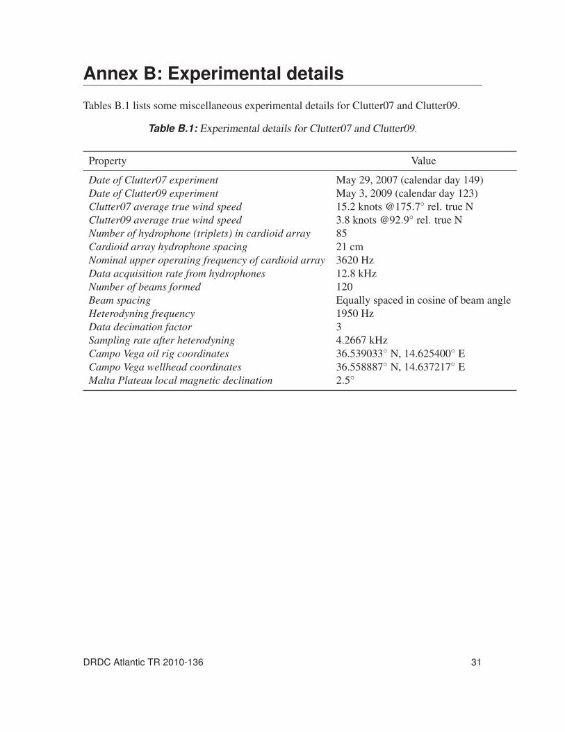
Annex B: Experimental details

Tables B.1 lists some miscellaneous experimental details for Clutter07 and Clutter09.

Table B.1: Experimental details for Clutter07 and Clutter09.

Property Value

Date of Clutter07 experiment May 29, 2007 (calendar day 149)

Date of Clutter09 experiment May 3, 2009 (calendar day 123)

Clutter07 average true wind speed 15.2 knots @175.7◦ rel. true N

Clutter09 average true wind speed 3.8 knots @92.9◦ rel. true N

Number of hydrophone (triplets) in cardioid array 85

Cardioid array hydrophone spacing 21 cm

Nominal upper operating frequency of cardioid array 3620 Hz

Data acquisition rate from hydrophones 12.8 kHz

Number of beams formed 120

Beam spacing Equally spaced in cosine of beam angle

Heterodyning frequency 1950 Hz

Data decimation factor 3

Sampling rate after heterodyning 4.2667 kHz

Campo Vega oil rig coordinates 36.539033◦ N, 14.625400◦ E

Campo Vega wellhead coordinates 36.558887◦ N, 14.637217◦ E

Malta Plateau local magnetic declination 2.5◦




Annex C: Reverberation statisticsC.1 DetectionWhen an active sonar ping is transmitted underwater, the receiver measures reverberation

even if echoes from strong reflectors – manmade or geological – are absent. If it is assumed

that this reverberation is caused by the sum of contributions from many scatterers, then the

instantaneous amplitude of the reverberation signal should have Gaussian statistics accord-

ing to the Central Limit Theorem. The envelope of the reverberation therefore follows a

Rayleigh distribution, and the intensity (squared envelope) follows an exponential distribu-

tion. Reverberation statistics are discussed in further detail in the next section (C.2), where

the assumption that Clutter09 reverberation intensity data is distributed exponentially is

also validated.

If the reverberation is stationary (constant average power) and the reverberation intensity

is assumed to follow an exponential distribution, a false alarm rate can be specified, where

from the detector standpoint, a false alarm indicates a detection caused by reverberation in

the absence of a legitimate echo return (contact). However, since the reverberation power

is not constant but rather decays with time, normalization of receiver data is required.

As depicted in Figure C.1, the (enveloped, matched-filtered) receiver time series data are

normalized using a split-window normalizer that estimates reverberation and background

noise power from samples of auxiliary data adjacent (separated by guard bands) to the

sample being normalized. Samples in the normalized data that exceed a specified threshold

(set by the false alarm rate requirement) are considered to be detections [5].

An automatic detector that uses split-window normalization was developed for Clutter09

by the author of [5]. Assuming exponentially distributed reverberation intensity data, a

probability of false alarm (PFA) of 1.0×10−6 was specified and used to determine a signal-

to-noise ratio (SNR) threshold of 13.82 (11.40 dB) using Equation C.8 which is introduced

later in this section. In normalizing the enveloped, matched-filtered time series with the

split-window method, the SNR of each sample is calculated, since each sample (instan-

taneous power) is divided by an estimate of surrounding noise power. The matched-filter

employed by the detector uses a parameter-generated replica of an LFM from 500–3500

Hz with a duration of 1.1 s, shaded using a raised cosine taper for the first and last 100 Hz

of the LFM.

Ideally, each echo is associated with a single detection; however, a single event, or echo,

can contain many raw detections, therefore a method of refining or clustering the detections

is required. Time clustering and beam clustering are performed to refine detections over

range and across bearing.

The detector starts by refining each beam time series individually (time clustering). For

each beam, the detection with the largest amplitude is isolated, and any other detections


Magnitude squared matched filter outputSample being normalized

GuardbandGuardband Auxiliary dataAuxiliary dataNormalizedsample

Estimate of time dependent noise background (reverb.) powerCompare to threshold

Figure C.1: Split-window normalizer used by the detector. Figure reconstructed from [5].

within 50 ms are considered to be associated. These detections are removed. This is

repeated for the next highest detection, and so on, so that each detection is separated from

other detections by at least 50 ms. Note that echoes with durations longer than 50 ms can

contain multiple refined detections.

Next, the detections are clustered across beams, to remove instances of echoes on multiple

beams caused by signal leakage into sidelobes. The assumed contact beam is the one with

the highest SNR detection, and instances of the detection on other beams are removed

from the detection list. Similar to time clustering, beam clustering starts with the highest

SNR (time-clustered) detection. Detections occurring within 10 ms on different beams are

candidates for association. For detections with SNR < 20 dB, any candidate detections

within 6 beams are associated. Detections with 20–25 dB SNR have candidate detections

within 8 beams associated, and for detections with SNR > 25 dB, candidate detections on

all beams are associated. As with time clustering, all associations are removed from the

list of detections, associations are determined for the next highest detection, and so on.

The cardioid left-right ambiguity suppression in NURC’s beamformer also has limitations,

so high SNR echoes may be observed on ambiguous beams. An ambiguous beam has

the same angle from end-fire as the contact beam, only it is on the opposite side of the

array. If a detection’s SNR > 18 dB, candidate detections on beams ambiguous with those

considered (according to SNR) in the last paragraph are also associated.


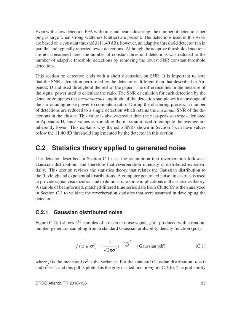
Even with a low detection PFA with time and beam clustering, the number of detections per

ping is large when strong scatterers (clutter) are present. The detections used in this work

are based on a constant threshold (11.40 dB), however, an adaptive threshold detector ran in

parallel and typically reported fewer detections. Although the adaptive threshold detections

are not considered here, the number of constant threshold detections was reduced to the

number of adaptive threshold detections by removing the lowest SNR constant threshold

detections.

This section on detection ends with a short discussion on SNR. It is important to note

that the SNR calculation performed by the detector is different than that described in Ap-

pendix D and used throughout the rest of the paper. The difference lies in the measure of

the signal power used to calculate the ratio. The SNR calculation for each detection by the

detector compares the instantaneous amplitude of the detection sample with an average of

the surrounding noise power to compute a ratio. During the clustering process, a number

of detections are reduced to a single detection which retains the maximum SNR of the de-

tections in the cluster. This value is always greater than the near-peak average calculated

in Appendix D, since values surrounding the maximum used to compute the average are

inherently lower. This explains why the echo SNRs shown in Section 5 can have values

below the 11.40 dB threshold implemented by the detector in this section.

C.2 Statistics theory applied to generated noiseThe detector described in Section C.1 uses the assumption that reverberation follows a

Gaussian distribution, and therefore that reverberation intensity is distributed exponen-

tially. This section reviews the statistics theory that relates the Gaussian distribution to

the Rayleigh and exponential distributions. A computer generated noise time series is used

to provide signal visualization and to demonstrate some implications of the statistics theory.

A sample of beamformed, matched-filtered time series data from Clutter09 is then analyzed

in Section C.3 to validate the reverberation statistics that were assumed in developing the

detector.

C.2.1 Gaussian distributed noise

Figure C.2(a) shows 216 samples of a discrete noise signal, g[n], produced with a random

number generator sampling from a standard Gaussian probability density function (pdf):

f(x; μ,σ2

)=

1√2πσ2

e−(x−μ)2

2σ2 (Gaussian pdf) (C.1)

where μ is the mean and σ2 is the variance. For the standard Gaussian distribution, μ = 0

and σ2 = 1, and this pdf is plotted as the gray dashed line in Figure C.2(b). The probability


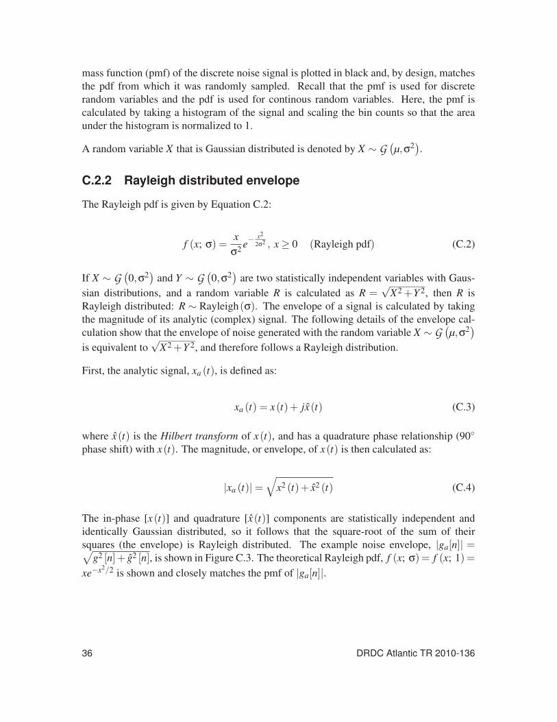
mass function (pmf) of the discrete noise signal is plotted in black and, by design, matches

the pdf from which it was randomly sampled. Recall that the pmf is used for discrete

random variables and the pdf is used for continous random variables. Here, the pmf is

calculated by taking a histogram of the signal and scaling the bin counts so that the area

under the histogram is normalized to 1.

A random variable X that is Gaussian distributed is denoted by X ∼ G(μ,σ2

).

C.2.2 Rayleigh distributed envelope

The Rayleigh pdf is given by Equation C.2:

f (x; σ) =x

σ2e−

x2

2σ2 , x ≥ 0 (Rayleigh pdf) (C.2)

If X ∼ G(0,σ2

)and Y ∼ G

(0,σ2

)are two statistically independent variables with Gaus-

sian distributions, and a random variable R is calculated as R =√

X2 +Y 2, then R is

Rayleigh distributed: R ∼ Rayleigh(σ). The envelope of a signal is calculated by taking

the magnitude of its analytic (complex) signal. The following details of the envelope cal-

culation show that the envelope of noise generated with the random variable X ∼ G(μ,σ2

)is equivalent to

√X2 +Y 2, and therefore follows a Rayleigh distribution.

First, the analytic signal, xa (t), is defined as:

xa (t) = x(t)+ jx(t) (C.3)

where x(t) is the Hilbert transform of x(t), and has a quadrature phase relationship (90◦phase shift) with x(t). The magnitude, or envelope, of x(t) is then calculated as:

|xa (t)|=√

x2 (t)+ x2 (t) (C.4)

The in-phase [x(t)] and quadrature [x(t)] components are statistically independent and

identically Gaussian distributed, so it follows that the square-root of the sum of their

squares (the envelope) is Rayleigh distributed. The example noise envelope, |ga[n]| =√g2 [n]+ g2 [n], is shown in Figure C.3. The theoretical Rayleigh pdf, f (x; σ) = f (x; 1) =

xe−x2/2 is shown and closely matches the pmf of |ga[n]|.


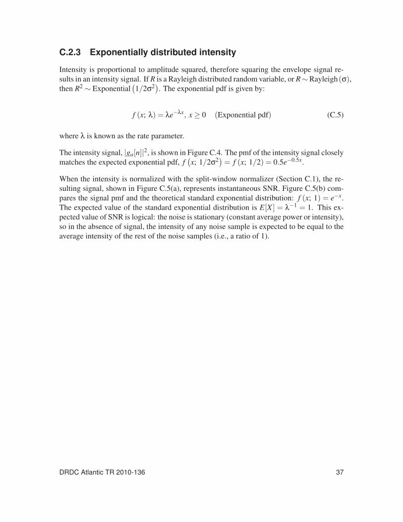
C.2.3 Exponentially distributed intensity

Intensity is proportional to amplitude squared, therefore squaring the envelope signal re-

sults in an intensity signal. If R is a Rayleigh distributed random variable, or R∼Rayleigh(σ),then R2 ∼ Exponential

(1/2σ2

). The exponential pdf is given by:

f (x; λ) = λe−λx, x ≥ 0 (Exponential pdf) (C.5)

where λ is known as the rate parameter.

The intensity signal, |ga[n]|2, is shown in Figure C.4. The pmf of the intensity signal closely

matches the expected exponential pdf, f(x; 1/2σ2

)= f (x; 1/2) = 0.5e−0.5x.

When the intensity is normalized with the split-window normalizer (Section C.1), the re-

sulting signal, shown in Figure C.5(a), represents instantaneous SNR. Figure C.5(b) com-

pares the signal pmf and the theoretical standard exponential distribution: f (x; 1) = e−x.

The expected value of the standard exponential distribution is E[X ] = λ−1 = 1. This ex-

pected value of SNR is logical: the noise is stationary (constant average power or intensity),

so in the absence of signal, the intensity of any noise sample is expected to be equal to the

average intensity of the rest of the noise samples (i.e., a ratio of 1).


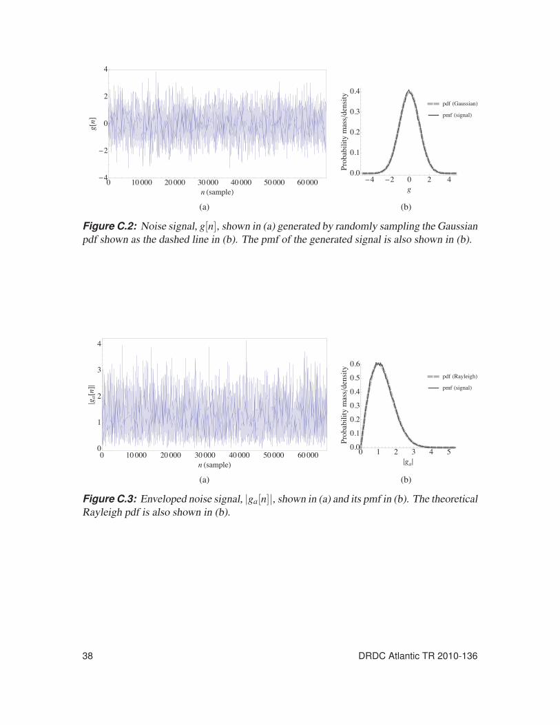
(a) (b)

Figure C.2: Noise signal, g[n], shown in (a) generated by randomly sampling the Gaussian

pdf shown as the dashed line in (b). The pmf of the generated signal is also shown in (b).

(a) (b)

Figure C.3: Enveloped noise signal, |ga[n]|, shown in (a) and its pmf in (b). The theoretical

Rayleigh pdf is also shown in (b).


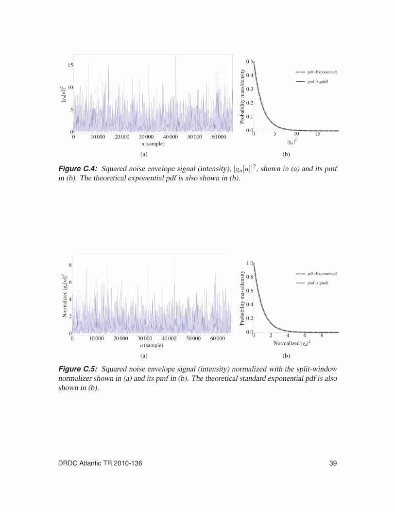
(a) (b)

Figure C.4: Squared noise envelope signal (intensity), |ga[n]|2, shown in (a) and its pmf

in (b). The theoretical exponential pdf is also shown in (b).

(a) (b)

Figure C.5: Squared noise envelope signal (intensity) normalized with the split-window

normalizer shown in (a) and its pmf in (b). The theoretical standard exponential pdf is also

shown in (b).


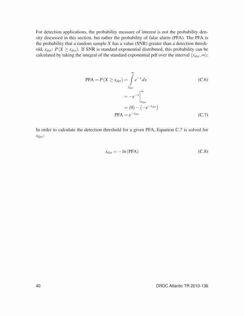
For detection applications, the probability measure of interest is not the probability den-

sity discussed in this section, but rather the probability of false alarm (PFA). The PFA is

the probability that a random sample X has a value (SNR) greater than a detection thresh-

old, xdet : P(X ≥ xdet). If SNR is standard exponential distributed, this probability can be

calculated by taking the integral of the standard exponential pdf over the interval (xdet ,∞):

PFA = P(X ≥ xdet) =

∞∫xdet

e−x dx (C.6)

=−e−x∣∣∣∣∞

xdet

= (0)− (−e−xdet)

PFA = e−xdet (C.7)

In order to calculate the detection threshold for a given PFA, Equation C.7 is solved for

xdet :

xdet =− ln(PFA) (C.8)


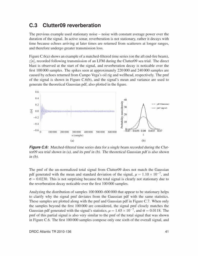
C.3 Clutter09 reverberationThe previous example used stationary noise – noise with constant average power over the

duration of the signal. In active sonar, reverberation is not stationary, rather it decays with

time because echoes arriving at later times are returned from scatterers at longer ranges,

and therefore undergo greater transmission loss.

Figure C.6(a) shows an example of a matched-filtered time series (on the aft end-fire beam),

z[n], recorded following transmission of an LFM during the Clutter09 sea trial. The direct

blast is observed at the start of the signal, and reverberation decay is noticable over the

first 100 000 samples. The spikes seen at approximately 220 000 and 240 000 samples are

caused by echoes returned from Campo Vega’s oil rig and wellhead, respectively. The pmf

of the signal is shown in Figure C.6(b), and the signal’s mean and variance are used to

generate the theoretical Gaussian pdf, also plotted in the figure.

(a) (b)

Figure C.6: Matched-filtered time series data for a single beam recorded during the Clut-

ter09 sea trial shown in (a), and its pmf in (b). The theoretical Gaussian pdf is also shown

in (b).

The pmf of the un-normalized total signal from Clutter09 does not match the Gaussian

pdf generated with the mean and standard deviation of the signal, μ = 1.10× 10−7, and

σ = 0.0230. This is not surprising because the total signal is clearly not stationary due to

the reverberation decay noticable over the first 100 000 samples.

Analyzing the distribution of samples 100 0000–600 000 that appear to be stationary helps

to clarify why the signal pmf deviates from the Gaussian pdf with the same statistics.

These samples are plotted along with the pmf and Gaussian pdf in Figure C.7. When only

the samples beyond the first 100 000 are considered, the signal pmf closely matches the

Gaussian pdf generated with the signal’s statistics, μ = 1.65×10−7, and σ = 0.0118. The

pmf of this partial signal is also very similar to the pmf of the total signal that was shown

in Figure C.6. The first 100 000 samples compose only one sixth of the overall signal, and


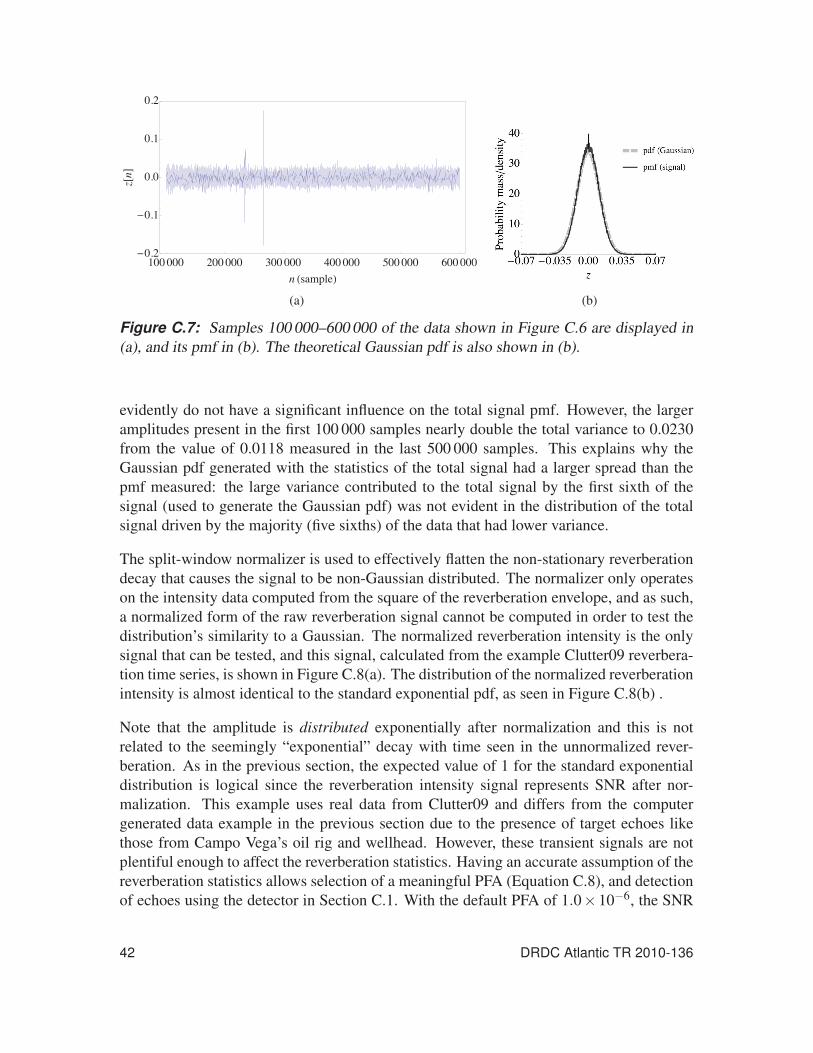
(a) (b)

Figure C.7: Samples 100 000–600 000 of the data shown in Figure C.6 are displayed in

(a), and its pmf in (b). The theoretical Gaussian pdf is also shown in (b).

evidently do not have a significant influence on the total signal pmf. However, the larger

amplitudes present in the first 100 000 samples nearly double the total variance to 0.0230

from the value of 0.0118 measured in the last 500 000 samples. This explains why the

Gaussian pdf generated with the statistics of the total signal had a larger spread than the

pmf measured: the large variance contributed to the total signal by the first sixth of the

signal (used to generate the Gaussian pdf) was not evident in the distribution of the total

signal driven by the majority (five sixths) of the data that had lower variance.

The split-window normalizer is used to effectively flatten the non-stationary reverberation

decay that causes the signal to be non-Gaussian distributed. The normalizer only operates

on the intensity data computed from the square of the reverberation envelope, and as such,

a normalized form of the raw reverberation signal cannot be computed in order to test the

distribution’s similarity to a Gaussian. The normalized reverberation intensity is the only

signal that can be tested, and this signal, calculated from the example Clutter09 reverbera-

tion time series, is shown in Figure C.8(a). The distribution of the normalized reverberation

intensity is almost identical to the standard exponential pdf, as seen in Figure C.8(b) .

Note that the amplitude is distributed exponentially after normalization and this is not

related to the seemingly “exponential” decay with time seen in the unnormalized rever-

beration. As in the previous section, the expected value of 1 for the standard exponential

distribution is logical since the reverberation intensity signal represents SNR after nor-

malization. This example uses real data from Clutter09 and differs from the computer

generated data example in the previous section due to the presence of target echoes like

those from Campo Vega’s oil rig and wellhead. However, these transient signals are not

plentiful enough to affect the reverberation statistics. Having an accurate assumption of the

reverberation statistics allows selection of a meaningful PFA (Equation C.8), and detection

of echoes using the detector in Section C.1. With the default PFA of 1.0×10−6, the SNR


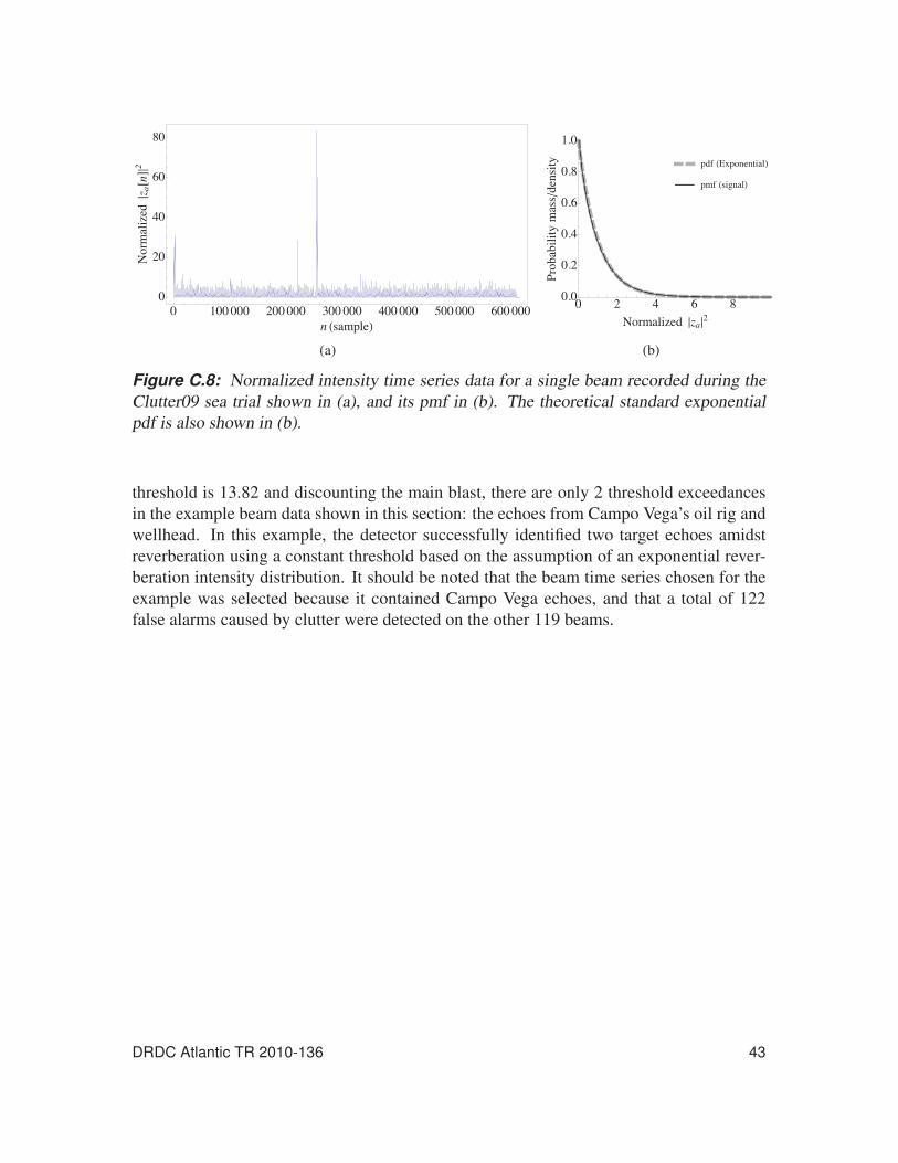
(a) (b)

Figure C.8: Normalized intensity time series data for a single beam recorded during the

Clutter09 sea trial shown in (a), and its pmf in (b). The theoretical standard exponential

pdf is also shown in (b).

threshold is 13.82 and discounting the main blast, there are only 2 threshold exceedances

in the example beam data shown in this section: the echoes from Campo Vega’s oil rig and

wellhead. In this example, the detector successfully identified two target echoes amidst

reverberation using a constant threshold based on the assumption of an exponential rever-

beration intensity distribution. It should be noted that the beam time series chosen for the

example was selected because it contained Campo Vega echoes, and that a total of 122

false alarms caused by clutter were detected on the other 119 beams.




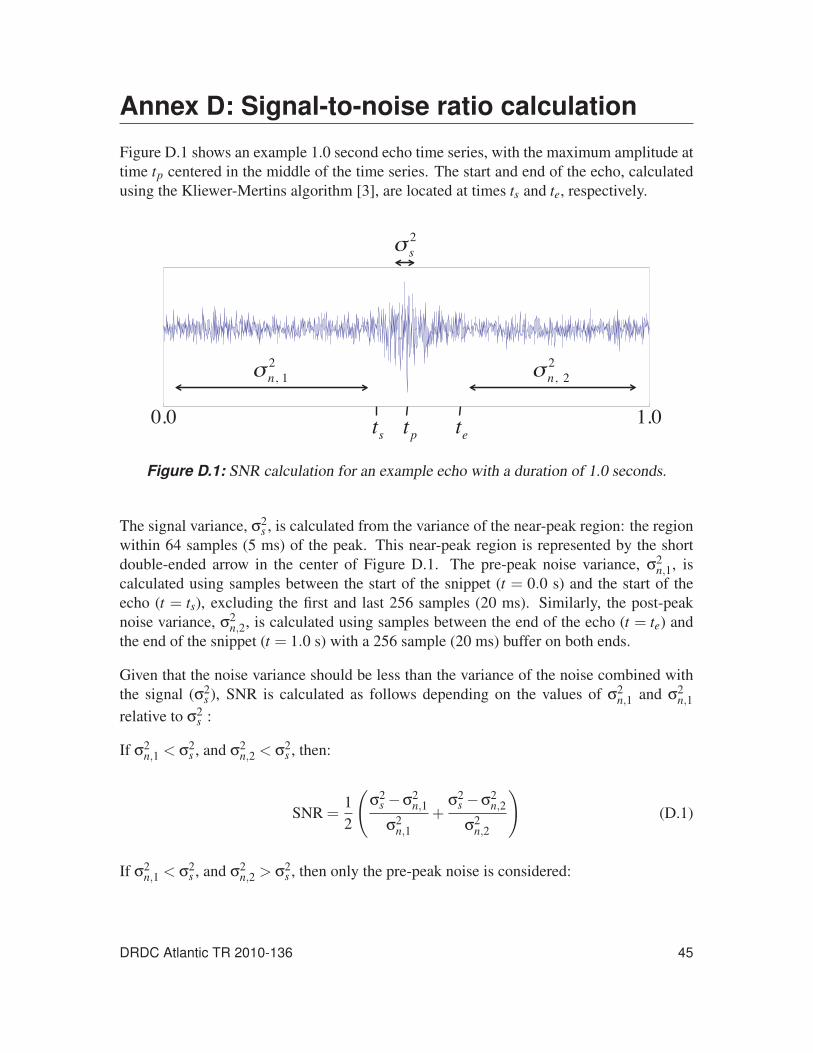
Annex D: Signal-to-noise ratio calculation

Figure D.1 shows an example 1.0 second echo time series, with the maximum amplitude at

time tp centered in the middle of the time series. The start and end of the echo, calculated

using the Kliewer-Mertins algorithm [3], are located at times ts and te, respectively.

0.0 1.0tp tets

s2

n, 12 n, 2

2

Figure D.1: SNR calculation for an example echo with a duration of 1.0 seconds.

The signal variance, σ2s , is calculated from the variance of the near-peak region: the region

within 64 samples (5 ms) of the peak. This near-peak region is represented by the short

double-ended arrow in the center of Figure D.1. The pre-peak noise variance, σ2n,1, is

calculated using samples between the start of the snippet (t = 0.0 s) and the start of the

echo (t = ts), excluding the first and last 256 samples (20 ms). Similarly, the post-peak

noise variance, σ2n,2, is calculated using samples between the end of the echo (t = te) and

the end of the snippet (t = 1.0 s) with a 256 sample (20 ms) buffer on both ends.

Given that the noise variance should be less than the variance of the noise combined with

the signal (σ2s ), SNR is calculated as follows depending on the values of σ2

n,1 and σ2n,1

relative to σ2s :

If σ2n,1 < σ2

s , and σ2n,2 < σ2

s , then:

SNR =1

2

(σ2

s −σ2n,1

σ2n,1

+σ2

s −σ2n,2

σ2n,2

)(D.1)

If σ2n,1 < σ2

s , and σ2n,2 > σ2

s , then only the pre-peak noise is considered:


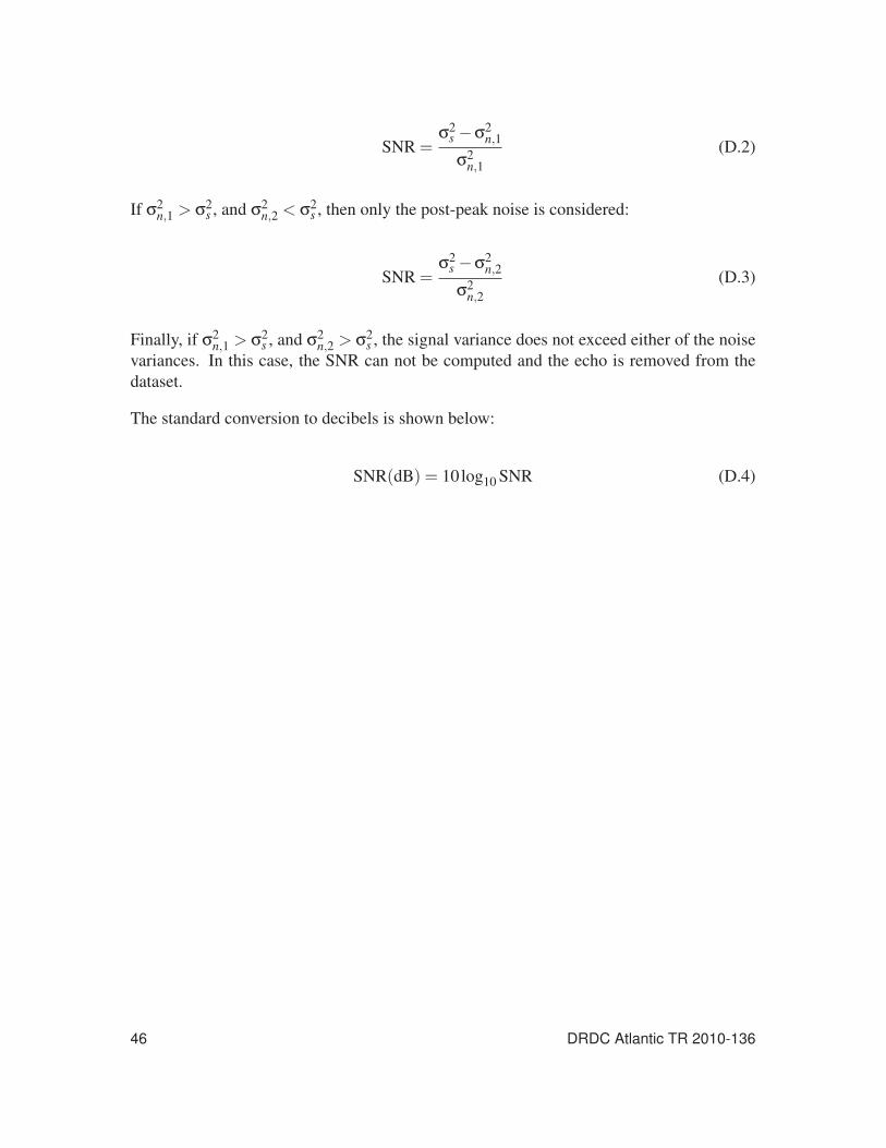
SNR =σ2

s −σ2n,1

σ2n,1

(D.2)

If σ2n,1 > σ2

s , and σ2n,2 < σ2

s , then only the post-peak noise is considered:

SNR =σ2

s −σ2n,2

σ2n,2

(D.3)

Finally, if σ2n,1 > σ2

s , and σ2n,2 > σ2

s , the signal variance does not exceed either of the noise

variances. In this case, the SNR can not be computed and the echo is removed from the

dataset.

The standard conversion to decibels is shown below:

SNR(dB) = 10log10 SNR (D.4)


Annex E: Feature listTable E.1: List of features ordered by discriminant score and overlap fraction ranking

methods.

Rank Feature (discriminant score) Feature (overlap fraction)

1 peak loudness value local min sub-band decay slope2 pre-attack noise peak loudness value global max sub-band attack slope3 loudness centroid global min sub-band decay slope4 pre-attack noise integrated loudness global mean sub-band decay slope5 psychoacoustic bin-to-bin difference peak loudness value6 local min sub-band decay slope pre-attack noise peak loudness value7 pre-attack noise loudness centroid pre-attack noise integrated loudness8 max sub-band attack slope loudness centroid9 global min sub-band decay slope frequency mean sub-band correlation

10 max sub-band correlation frequency psychoacoustic bin-to-bin difference11 global mean sub-band decay slope global min sub-band decay slope frequency12 global min sub-band decay slope pre-attack noise loudness centroid13 min sub-band correlation min sub-band correlation14 min sub-band correlation frequency max sub-band correlation frequency15 mean sub-band correlation global min sub-band decay time16 global min sub-band attack time global min sub-band attack time17 global max sub-band decay time frequency local max sub-band decay slope frequency18 pre-attack noise peak loudness frequency min sub-band correlation frequency19 peak loudness frequency peak loudness frequency20 local max sub-band decay slope frequency pre-attack noise peak loudness frequency21 global min sub-band attack time frequency local min sub-band attack slope frequency22 local min sub-band attack slope frequency global max sub-band decay time frequency23 global max sub-band decay slope global max sub-band decay slope frequency24 global max sub-band attack slope global min sub-band attack slope frequency25 local mean sub-band decay time global max sub-band attack slope frequency26 local max sub-band decay time global max sub-band decay slope27 global min sub-band decay time global min sub-band attack time frequency28 local max sub-band decay time frequency global mean sub-band decay time29 global min sub-band attack slope local mean sub-band decay time30 psychoacoustic MSBR local max sub-band decay time31 local max sub-band attack time global min sub-band attack slope

Continued on next page –


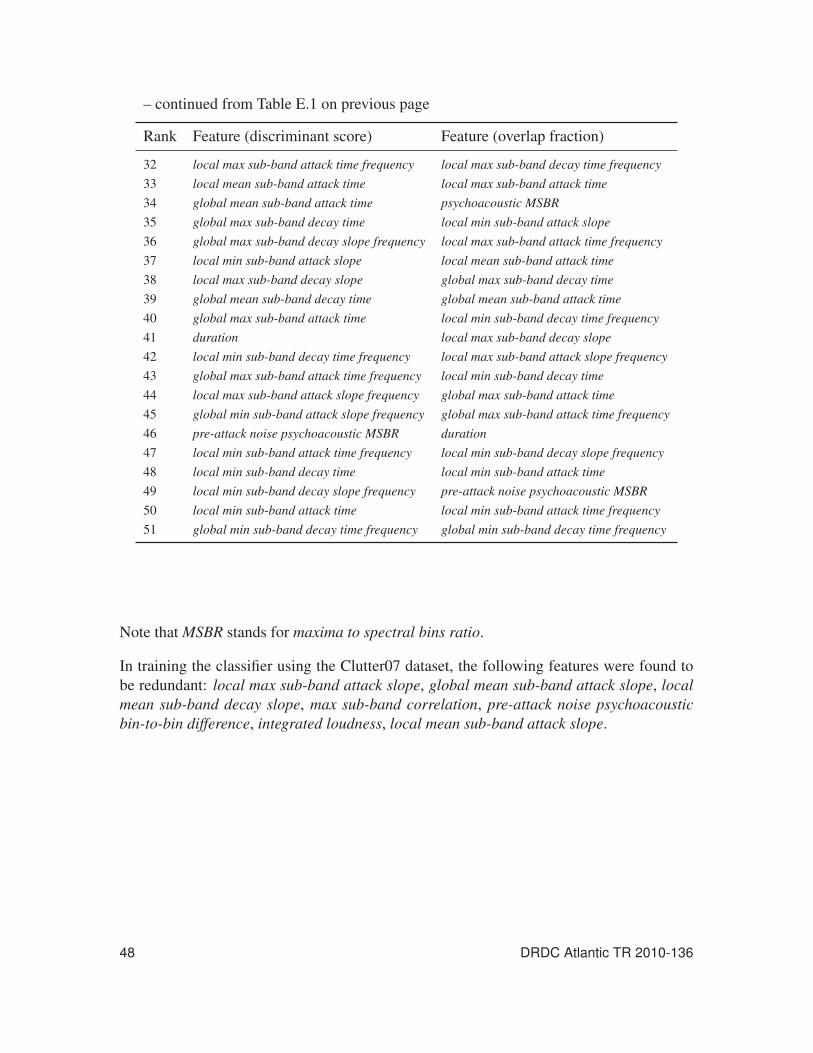
– continued from Table E.1 on previous page

Rank Feature (discriminant score) Feature (overlap fraction)

32 local max sub-band attack time frequency local max sub-band decay time frequency33 local mean sub-band attack time local max sub-band attack time34 global mean sub-band attack time psychoacoustic MSBR35 global max sub-band decay time local min sub-band attack slope36 global max sub-band decay slope frequency local max sub-band attack time frequency37 local min sub-band attack slope local mean sub-band attack time38 local max sub-band decay slope global max sub-band decay time39 global mean sub-band decay time global mean sub-band attack time40 global max sub-band attack time local min sub-band decay time frequency41 duration local max sub-band decay slope42 local min sub-band decay time frequency local max sub-band attack slope frequency43 global max sub-band attack time frequency local min sub-band decay time44 local max sub-band attack slope frequency global max sub-band attack time45 global min sub-band attack slope frequency global max sub-band attack time frequency46 pre-attack noise psychoacoustic MSBR duration47 local min sub-band attack time frequency local min sub-band decay slope frequency48 local min sub-band decay time local min sub-band attack time49 local min sub-band decay slope frequency pre-attack noise psychoacoustic MSBR50 local min sub-band attack time local min sub-band attack time frequency51 global min sub-band decay time frequency global min sub-band decay time frequency

Note that MSBR stands for maxima to spectral bins ratio.

In training the classifier using the Clutter07 dataset, the following features were found to

be redundant: local max sub-band attack slope, global mean sub-band attack slope, localmean sub-band decay slope, max sub-band correlation, pre-attack noise psychoacousticbin-to-bin difference, integrated loudness, local mean sub-band attack slope.


Distribution list


Internal distribution3 Paul C. Hines (1 hard copy + 2 soft copies)

3 DRDC Atlantic Library (1 hard copy + 2 soft copies)

1 Stefan M. Murphy (1 hard copy)

1 H/Underwater Sensing

1 H/Technology Demonstration

1 H/Maritime Information & Combat Systems

1 GL/Maritime Environmental Awareness

1 Jeff Scrutton

1 Garfield Mellema

1 Dan Peters

1 Vincent Myers

1 Senior Military Officer

Total internal copies: 16

External distributionDepartment of National Defence

1 DRDKIM

The following 6 copies sent c/o:

CFB Halifax, PO BOX 99000, Stn Forces, NS B3K 5X5

1 ADAC(A) – Commanding Officer

1 CFMWC – Commanding Officer

1 CFNOS – Commanding Officer


1 MOG5 – Commanding Officer

1 PSU HALIFAX – Commanding Officer

1 TRINITY – Commanding Officer

Canadian recipients

1 Library and Archives Canada

Attn: Military Archivist, Government Records Branch

International recipients

1 Dr. Ellen Livingston

Office of Naval Research Global

Edison House

223 Old Marylebone Road

London NW1 5TH

UNITED KINGDOM

1 Dr. James Pitton

Applied Physics Laboratory

University of Washington

1013 NE 40th Street

Box 355640

Seattle, WA 98105-6698

USA

Total external copies: 10

Total copies: 26


DOCUMENT CONTROL DATA(Security classification of title, body of abstract and indexing annotation must be entered when document is classified)

1. ORIGINATOR (The name and address of the organization preparing thedocument. Organizations for whom the document was prepared, e.g. Centresponsoring a contractor’s report, or tasking agency, are entered in section 8.)

Defence R&D Canada – AtlanticPO Box 1012, Dartmouth NS B2Y 3Z7, Canada

2. SECURITY CLASSIFICATION (Overallsecurity classification of the documentincluding special warning terms if applicable.)

UNCLASSIFIED

3. TITLE (The complete document title as indicated on the title page. Its classification should be indicated by the appropriateabbreviation (S, C or U) in parentheses after the title.)


4. AUTHORS (Last name, followed by initials – ranks, titles, etc. not to be used.)

Murphy, S. M.; Hines, P. C.

5. DATE OF PUBLICATION (Month and year of publication ofdocument.)

November 2010

6a. NO. OF PAGES (Totalcontaining information.Include Annexes,Appendices, etc.)

66

6b. NO. OF REFS (Totalcited in document.)

10

7. DESCRIPTIVE NOTES (The category of the document, e.g. technical report, technical note or memorandum. If appropriate, enterthe type of report, e.g. interim, progress, summary, annual or final. Give the inclusive dates when a specific reporting period iscovered.)

Technical Report

8. SPONSORING ACTIVITY (The name of the department project office or laboratory sponsoring the research and development –include address.)

Defence R&D Canada – AtlanticPO Box 1012, Dartmouth NS B2Y 3Z7, Canada

9a. PROJECT OR GRANT NO. (If appropriate, the applicableresearch and development project or grant number underwhich the document was written. Please specify whetherproject or grant.)

11cb04

9b. CONTRACT NO. (If appropriate, the applicable number underwhich the document was written.)

ONR Grant N00014-09-1-0426

10a. ORIGINATOR’S DOCUMENT NUMBER (The officialdocument number by which the document is identified by theoriginating activity. This number must be unique to thisdocument.)


10b. OTHER DOCUMENT NO(s). (Any other numbers which maybe assigned this document either by the originator or by thesponsor.)

11. DOCUMENT AVAILABILITY (Any limitations on further dissemination of the document, other than those imposed by securityclassification.)( X ) Unlimited distribution( ) Defence departments and defence contractors; further distribution only as approved( ) Defence departments and Canadian defence contractors; further distribution only as approved( ) Government departments and agencies; further distribution only as approved( ) Defence departments; further distribution only as approved( ) Other (please specify):

12. DOCUMENT ANNOUNCEMENT (Any limitation to the bibliographic announcement of this document. This will normally correspondto the Document Availability (11). However, where further distribution (beyond the audience specified in (11)) is possible, a widerannouncement audience may be selected.)

Unlimited

13. ABSTRACT (A brief and factual summary of the document. It may also appear elsewhere in the body of the document itself. It is highlydesirable that the abstract of classified documents be unclassified. Each paragraph of the abstract shall begin with an indication of thesecurity classification of the information in the paragraph (unless the document itself is unclassified) represented as (S), (C), or (U). It isnot necessary to include here abstracts in both official languages unless the text is bilingual.)

Active sonar systems are used to detect underwater manmade objects of interest (targets) thatare too quiet to be reliably detected with passive sonar. In coastal waters, the performance of ac-tive sonar is degraded by false alarms caused by echoes returned from geological seabed struc-tures (clutter ) found in these shallow regions. To reduce false alarms, a method of distinguishingtarget echoes from clutter echoes is required. Research has demonstrated that perceptual signalfeatures similar to those employed in the human auditory system can be used to automaticallydiscriminate between target and clutter echoes, thereby improving sonar performance by reduc-ing the number of false alarms.

An active sonar experiment on the Malta Plateau was conducted during the Clutter07 sea trialand repeated during the Clutter09 sea trial. Broadband sources were used to transmit linearFM sweeps (600–3400 Hz) and a cardioid towed-array was used as the receiver. The datasetconsists of over 95 000 pulse-compressed echoes returned from two targets and many geologicalclutter objects.

These echoes are processed using an automatic classifier that quantifies the timbre of eachecho using a number of perceptual signal features. Using echoes from 2007, the aural classifieris trained to establish a boundary between targets and clutter in the feature space. Temporalrobustness is then investigated by testing the classifier on echoes from the 2009 experiment.

14. KEYWORDS, DESCRIPTORS or IDENTIFIERS (Technically meaningful terms or short phrases that characterize a document and couldbe helpful in cataloguing the document. They should be selected so that no security classification is required. Identifiers, such asequipment model designation, trade name, military project code name, geographic location may also be included. If possible keywordsshould be selected from a published thesaurus. e.g. Thesaurus of Engineering and Scientific Terms (TEST) and that thesaurus identified.If it is not possible to select indexing terms which are Unclassified, the classification of each should be indicated as with the title.)

active sonarclassificationpattern recognitionaural classificationdetectionclutter


Documents

TR 2010-136 A1b - Defence Research Reportscradpdf.drdc-rddc.gc.ca/PDFS/unc111/p535180_A1b.pdf · These echoes are processed using an automatic classiﬁer that quantiﬁes the timbre