Traffic Analysis for the Calibration of Risk Assessment Methods

B. R. Calder∗ K. Schwehr†

Abstract

In order to provide some measure of the uncertainty in-herent in the sorts of charting data that are providedto the end-user, we have previously proposed risk mod-els that measure the magnitude of the uncertainty fora ship operating in a particular area. Calibration ofthese models is essential, but the complexity of themodels means that we require detailed information onthe sorts of ships, traffic patterns and density withinthe model area to make a reliable assessment. In the-ory, the ais system should provide this information fora suitably instrumented area. We consider the problemof converting, filtering and analysing the raw ais trafficto provide statistical characterizations of the traffic ina particular area, and illustrate the method with datafrom 2008-10-01 through 2008-11-30 around Norfolk,VA. We show that it is possible to automatically con-struct aggregate statistical characteristics of the port,resulting in distributions of transit location, termina-tion and duration by vessel category, as well as type oftraffic, physical dimensions, and intensity of activity.We also observe that although 60 days give us suffi-cient data for our immediate purposes, a large propor-tion of it—up to 52% by message volume—must beconsidered dubious due to difficulties in configuration,maintenance and operation of ais transceivers.

1 Introduction

Assessing the risk to a vessel of transiting or anchoringin a given area is a fundamental task for the user ofhydrographic data. A sufficiently nuanced analysis ofrisk is one way to communicate, to the user, the degreeof uncertainty in the data being presented, providinga much better means to analyze and understand thecompleteness, accuracy and validity of the navigationalproduct for an individual than current methods suchas source or reliability diagrams, or their equivalents inelectronic products (e.g., Zones of Confidence [ZOCs]).

∗Center for Coastal and Ocean Mapping and noaa-unh Joint

Hydrographic Center, University of New Hampshire, Durham

NH 03824, USA. E-mail: brc@ccom.unh.edu

†Address as above; e-mail schwehr@ccom.unh.edu

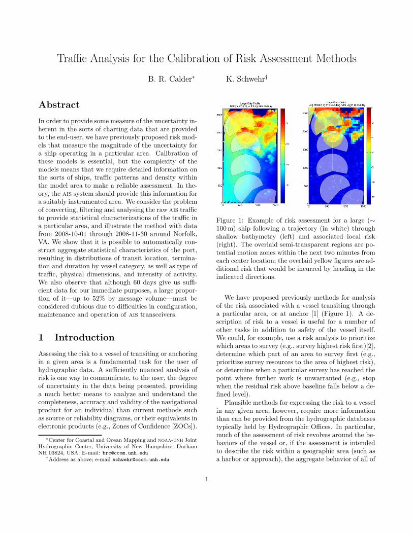
Figure 1: Example of risk assessment for a large (∼100 m) ship following a trajectory (in white) throughshallow bathymetry (left) and associated local risk(right). The overlaid semi-transparent regions are po-tential motion zones within the next two minutes fromeach center location; the overlaid yellow figures are ad-ditional risk that would be incurred by heading in theindicated directions.

We have proposed previously methods for analysisof the risk associated with a vessel transiting througha particular area, or at anchor [1] (Figure 1). A de-scription of risk to a vessel is useful for a number ofother tasks in addition to safety of the vessel itself.We could, for example, use a risk analysis to prioritizewhich areas to survey (e.g., survey highest risk first)[2],determine which part of an area to survey first (e.g.,prioritize survey resources to the area of highest risk),or determine when a particular survey has reached thepoint where further work is unwarranted (e.g., stopwhen the residual risk above baseline falls below a de-fined level).

Plausible methods for expressing the risk to a vesselin any given area, however, require more informationthan can be provided from the hydrographic databasestypically held by Hydrographic Offices. In particular,much of the assessment of risk revolves around the be-haviors of the vessel or, if the assessment is intendedto describe the risk within a geographic area (such asa harbor or approach), the aggregate behavior of all of

1

the traffic in the area. Other issues such as preferredtransit lanes, traffic control measures and local climaticconditions are also important. Unfortunately, this vi-tal information is typically either poorly understood ordifficult to obtain.

The Automatic Identification System (ais) is a vhfship-to-ship and ship-to-shore messaging system de-signed to pass vessel information. The primary goalof the initial ais specification was to assist with safetyof navigation by improving the situational awareness ofall mariners. ais is specified by International Telecom-munication Union Recommendation (itu-r) M.1371-3[3].

The system uses two 9600bps radio transceivers inthe 160MHz band with 1 to 12.5W power. This RFchannel limits the amount of data and gives maximumranges from 5 to 400km with 25–50km being typi-cal with most configurations. Each ship is equippedwith a transceiver that operates in a Self-OrganizingTime Division Multiple Access (sotdma) network toexchange messages. There are currently two classesof transceivers. The first, Class A, uses 12.5W trans-mission power and is higher priority and more config-urable than Class B, which is limited to 2W powerand must be programed by a vendor. Class B sys-tems also transmit position reports and ship informa-tion at a lower rate. Operators of Class A equipmentare expected to enter data into the device either withthe Minimum Keyboard Display (mkd) or through anElectronic Charting System (ecs).

ais has been in use since 2001, with mandatorycarriage requirements for new Safety Of Life At Sea(solas) class vessels since 2002-07-01. Carriage re-quirements are continuing to evolve with more vesseltypes likely to be required to carry ais transceivers inthe future. Even if it is not required, many marinerschoose to add ais transceivers to their vessels.

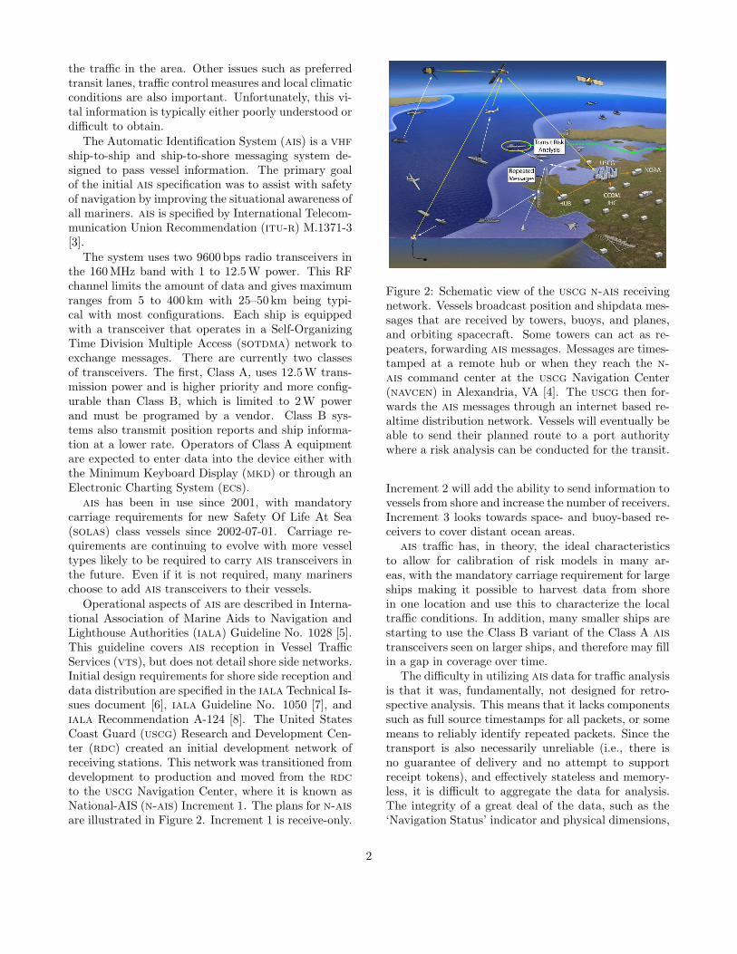
Operational aspects of ais are described in Interna-tional Association of Marine Aids to Navigation andLighthouse Authorities (iala) Guideline No. 1028 [5].This guideline covers ais reception in Vessel TrafficServices (vts), but does not detail shore side networks.Initial design requirements for shore side reception anddata distribution are specified in the iala Technical Is-sues document [6], iala Guideline No. 1050 [7], andiala Recommendation A-124 [8]. The United StatesCoast Guard (uscg) Research and Development Cen-ter (rdc) created an initial development network ofreceiving stations. This network was transitioned fromdevelopment to production and moved from the rdcto the uscg Navigation Center, where it is known asNational-AIS (n-ais) Increment 1. The plans for n-aisare illustrated in Figure 2. Increment 1 is receive-only.

Figure 2: Schematic view of the uscg n-ais receivingnetwork. Vessels broadcast position and shipdata mes-sages that are received by towers, buoys, and planes,and orbiting spacecraft. Some towers can act as re-peaters, forwarding ais messages. Messages are times-tamped at a remote hub or when they reach the n-ais command center at the uscg Navigation Center(navcen) in Alexandria, VA [4]. The uscg then for-wards the ais messages through an internet based re-altime distribution network. Vessels will eventually beable to send their planned route to a port authoritywhere a risk analysis can be conducted for the transit.

Increment 2 will add the ability to send information tovessels from shore and increase the number of receivers.Increment 3 looks towards space- and buoy-based re-ceivers to cover distant ocean areas.

ais traffic has, in theory, the ideal characteristicsto allow for calibration of risk models in many ar-eas, with the mandatory carriage requirement for largeships making it possible to harvest data from shorein one location and use this to characterize the localtraffic conditions. In addition, many smaller ships arestarting to use the Class B variant of the Class A aistransceivers seen on larger ships, and therefore may fillin a gap in coverage over time.

The difficulty in utilizing ais data for traffic analysisis that it was, fundamentally, not designed for retro-spective analysis. This means that it lacks componentssuch as full source timestamps for all packets, or somemeans to reliably identify repeated packets. Since thetransport is also necessarily unreliable (i.e., there isno guarantee of delivery and no attempt to supportreceipt tokens), and effectively stateless and memory-less, it is difficult to aggregate the data for analysis.The integrity of a great deal of the data, such as the‘Navigation Status’ indicator and physical dimensions,

2

particularly draught, is also reliant on the user makingappropriate adjustments to reflect the ship’s currentstatus. As with all manual systems, this leads to po-tential for confusion, misinterpretation and inappropri-ate configuration [9]. It is relatively simple to do roughtraffic density or intensity analysis [10], but much moredifficult to extract stateful synoptic descriptions of theactual behaviors of the various classes of traffic withina given area. If we wish to calibrate risk models—oreven to understand the traffic in a particular area—weneed to parse a little more finely.

We therefore propose a scheme for automatic pro-cessing of n-ais traffic in a constrained area that pre-parses the data from the nmea-encoded form of the aismessage format [11], applies rough spatial filtering toselect a particular area, and then repackages the datain a relational database [12, 13]. The database is thenpre-filtered to sanitize the contents; the intent is thatafter the sanitization process, the database should beable to answer queries about the traffic without theuser having to take special precautions on the results(such as looking for duplicates or missing information).We next parse the database in a number of differentways to elicit the behavior of traffic in the area of in-terest, including the physical dimensions of ships inbroad traffic classes, the duration, frequency, locationand endpoints of individual transits, and patterns ofarrival and departure time, vessel affinity and dockactivity intensity for automatically identified areas oftransit endpoint clustering. We stratify the behaviorsby traffic categories and dock/anchorage areas to bet-ter tune models of particular classes, typically the largecommercial traffic, which may be more important inthe overall controls on traffic in the area of interest.Our goal is to establish a series of hierarchically re-lated statistical models that can be used to simulatethe behaviors of traffic in the area of interest.

We illustrate these techniques in the case of theports of Norfolk and Hampton Roads, VA for the pe-riod between 2008-10-01 and 2008-11-30, and describethe difficulties we encountered in processing the data.We show that there are distinct patterns of durationof transits, significant class-specific clustering in thephysical characteristics of ships in the area, their des-tinations, and their operating areas that can be ex-ploited to simplify the resulting models. We observethat it is not possible to carry out the same analysisfor all classes of traffic in the area, since many classeshave either very few members or limited structure intheir behavior patterns. In these cases we show thatwe can summarize the aggregate behavior of the classwith simpler models that may not provide high fidelitymodeling of the total behavior, but provide sufficient

information to allow a reasonable description of the neteffect.

The presence and adoption of Class B transceivers isa question of current interest. We investigate this byconsidering the information from San Francisco, CAduring the same period, and show that although in-creasing numbers of Class B transceivers are observed,their relative abundance is still very small.

Finally, we provide some comments on the difficul-ties in processing ais data to characterize traffic andwhat might be done about it in the future. We alsoprovide some perspective on the future of traffic sim-ulation models derived from this work, and their usein risk models to assess uncertainty for the user, pri-oritize areas for resurvey and calibrate survey effort inthe field.

2 Methods

2.1 Pre-Processing and Database Gen-

eration

At present, there are 26 Message Identifiers denotingcategories of ais messages out of 64 total possible iden-tifiers. Our vessel traffic analysis uses the three ClassA position reports: 1) Scheduled position report, 2)Assigned scheduled position report, and 3) Special po-sition report—response to interrogation. For this anal-ysis, all position report types are treated as equivalent.ais message 5, ‘Static and Voyage related data’ (‘ship-data’), is used to obtain the vessel name, type/cargo,draught, and dimensions.

The messages were recorded from the uscg n-aisIncrement 1 network using the ‘with-out duplicates’mode [4], meaning that n-ais will only give one mes-sage even if it received at multiple towers. Messages arestored in uscg format 0—an extension to nmea-0183[14] that allows for additional metadata to be addedto the end of each line [15]. The extension adds fieldsfor the receive station, signal strength, slot number,time of arrival, and a unix utc timestamp. Each dayof messages is compressed with bzip2 [16] to approxi-mately 30% of the original data volume.

The next set of steps convert the position messagesand shipdata reports to a relational database. We usenoaadata [17] to convert to a sqlite [12] database inthis instance.

The position messages are extracted and clippedto a bounding box spanning 76◦54′W, 36◦12′N to75◦6′W, 37◦24′N. We chose the bounding box tocover the approaches to Chesapeake Bay through toNewport News and Norfolk, VA. The retained mes-

3

b003669730 r003669934 r05CCPH1b003669794 r003669935 r05RCHI1b2003669982 r003669936 r05RMSQ1r003381010 r003669937 r05RTUC1r003381012 r003669938 r05SOIN1r003381014 r003669939 r05XDCJ1r003669931 r003669957 r3669961r003669932 r003669959 rNDBC44014r003669933 r01SCST1

Table 1: n-ais stations covering the study area. Bases-tations start with ‘b’ and receive-only stations startwith ‘r’.

sages are then inserted into the database by theais build sqlite.py script in noaadata.

From the position messages received, a list of uniquestations receiving packets from the study area is gen-erated. The shipdata messages are then culled tothose received from the 26 stations (Table 1) that pro-vided positions within the study bounding box, andare converted to a normalized form. The raw mes-sage comes across the network in two separate nmeastrings that may be interspersed with other nmea mes-sages. The normal form violates the nmea-0183 for-mat by converting the multiple lines to one long sin-gle sentence line. The normal form is then passed toais build sqlite.py and added to the database.

The noaadata software only does simple checks ofthe expected message sizes to check for corrupted data.However, it does not do any packet inspection to rejectnonsensical content, leaving it to the data condition-ing steps to dig into the packet content and look atrelationships between packets to provide appropriatefiltering.

2.2 Data Conditioning

In order to make the analysis of the traffic data sim-pler, we first pre-filter the database to condition thebehavior of the data, but preserve the integrity of thedata by maintaining a reserve table for each data mes-sage type, into which we insert all data points thatare filtered from the primary tables. In order to main-tain information on the filtering within the database,we also construct a table to hold a text description ofeach filter that is applied, along with a reference num-ber. As we filter, we keep records of which unique IDsare removed from the data tables and maintain this in-formation in a third table within the database; subrou-tines of the main filtering code automate this processto ensure traceability. This mechanism ensures that wecan recover evidence of which data points were elimi-

nated for each reason, and recover them if required.As the first stage of data triage, we attempt to en-

sure that the data meets the requirements of the itustandards for ais [3]. Each ship is identified by a Mar-itime Mobile Service Identity (mmsi) number, a struc-tured identifier where the first digit indicates the re-gional origin of the ship (or at least where it is regis-tered), and the next two digits provide a country iden-tified within the general region. In particular, mmsisstarting with a zero or one are not meant to be assignedto general shipping, and no ships should be using acountry code not currently assigned. We therefore ex-tract the country component of the mmsi and match itagainst the currently assigned code table, eliminatingthose position and shipdata reports that do not matchthe list.

Next, we apply simple sanity checks to ensure thatall ship mmsis that appear in the position messagesalso appear in the shipdata messages, and vice versa.This condition of bijection between the two sets canbe violated if a remote tower picks up passing shipposition messages but no shipdata messages or viceversa, and is not readily identifiable at the databasebuild stage.

Third, we filter out all ships with very few positionreports, since they do not contribute significantly tothe traffic in a harbor. The limit of how many pointsare sufficient is essentially arbitrary; in this case, wecull all mmsis that appear in fewer than 30 positionmessages.

Next, we consider the static data for a ship thatshould be consistent in all situations: the mmsi, theimo number (if present), the ship’s name and callsign.Since this data is essentially free-form, there are a num-ber of ways in which it can be entered. The name, forexample, can be arbitrarily padded with spaces, or ‘endof string’ characters (represented by ‘@’). Even whenthese are controlled, however, we find numerous in-stances of ships whose names change lexicographically,although not semantically (‘MT MITCHELL’ to ‘MT.MITCHELL’ for example), or where random bit errorsin the radio transmission result in significant modifi-cations to the data stream. While it is possible thatsome of these could be resolved by human interaction,it is notoriously difficult to do approximate matching offree-form text like this automatically. In order to keepthe processing simple and efficient, and acknowledgingthat these situations are limited within the corpus, wechoose to simply filter all occurrences.

Fifth, we examine the ‘Ship and Cargo’ specificationassociated with the shipdata messages, and eliminateall traffic that is not in an appropriately defined cat-egory. This filtering is approximate, since there is no

4

restriction on the category that the vessel sets, andindeed one vessel can belong to multiple categories atdifferent times depending on what cargo it is carrying,and the role it is playing at the time (e.g., a tug canchange category to ‘towing’ once it is associated withits ship, and a ‘pleasure craft’ could conceivably changeto ‘fishing’ to indicate current use). Using values fromthe reserved sections, however, clearly indicates a mis-configured transceiver, and we filter all records fromsuch sources.

Next, we eliminate all traffic from repeater stations.In theory, it would be possible to use repeater trafficas a means to bolster questionable traffic, or extendthe range at which ships become visible but difficultieswith timestamping as presented limit this in practice.It is possible that these difficulties might be resolvedby detailed processing of embedded time informationthat occasionally appears in the data packets, but wehave not pursued this in the current work.

Finally, we consider the consistency and stability ofthe static ship dimension data. In the shipdata mes-sages, each ship broadcasts a length and breadth di-mension (specified as two components so that the po-sition of the primary source of position reports canbe identified), as well as an estimate of the draught.While we might expect that the draught of the shipwill change over time, there is little reason to believethat the overall dimensions should, at least unless thereis a corresponding change in the ‘Ship and Cargo’ valuebeing broadcast simultaneously. (For example, a tugthat takes a barge in tow might change its dimensionsto reflect the size of the combined entity.) We there-fore stratify by mmsi and ‘Ship and Cargo’ declared,and within each group compute the mean and stan-dard deviation of the declared length and breadth. Inorder to robustify the estimates, we apply a simple out-lier removal algorithm by ignoring all packets that areoutwith three standard deviations of the unconstrainedmean, and then recomputing the mean and standarddeviation. We consider the remaining packets to bedubious if there are fewer than 1% of the total packetsremaining in the estimate, or if the standard deviationis greater than 10% of the mean value in either dimen-sion, or if the length to breadth ratio is lower than 2.0(which is extremely unusual for most traffic, but char-acteristic of vessels with misconfigured receivers thathave swapped one or more of the measurements). Fi-nally, we filter all ships that have draught set to zero,since they have no useful information for our currentpurpose (draught and derived underkeel clearance arecritical for the sort of risk assessment models that areour ultimate goal). A surprising number of ships fallinto this category, including many super-yachts, but

also some commercial traffic where this is unexpected.

2.3 Transit Construction

The foundation for understanding the behavior of traf-fic in any given area is to be able to associate some se-mantics, which we cannot observe, with the data thatwe can. The most basic semantic structure is to dividethe contiguous sequence of position reports into a setof transits.

The term ‘transit’ admits multiple possible defini-tions. We interpret it here to mean a sequence of posi-tion reports from a particular ship, without significanttime gaps, which show some level of purposeful mo-tion. Typically, a transit starts when the ship is firstpicked up by the seaward most ais tower in the area,and finishes when the ship either goes to anchor, or tiesup at a pier. (We consider the case of a ship that goesto anchor for a period and then continues to the dockto be two transits.) Along the way, it is possible thatwe can lose contact with a ship for a period of time,and consequently we have to allow for time gaps in thesequence but ensure that too long a time gap is con-sidered to be a separate transit. If the ship disappearsfor a significant length of time, we have no guaranteethat is doing the same thing when it returns as it waswhen it disappeared.

In theory, transit detection is trivial for ais: the‘Navigation Status’ component of the shipdata mes-sages should provide an indication of when the shipis underway, moored, at anchor, etc. Unfortunately,however, because this information is set manually bythe bridge watch, it is typically not entirely reliable.We frequently see examples where the status is changedfrom ‘moored’ to ‘underway’ significantly after the shipis clearly moving (and vice versa); where the status isset to ‘underway’ though the ship does not move morethan 10m in any direction for 60 days; or where thestatus changes with the bridge watch.

Similarly, it should be possible to detect consistentmotion by estimating the variation of position reportsover time. This requires, however, choice of an essen-tially arbitrary set of parameters, making it difficult toautomate.

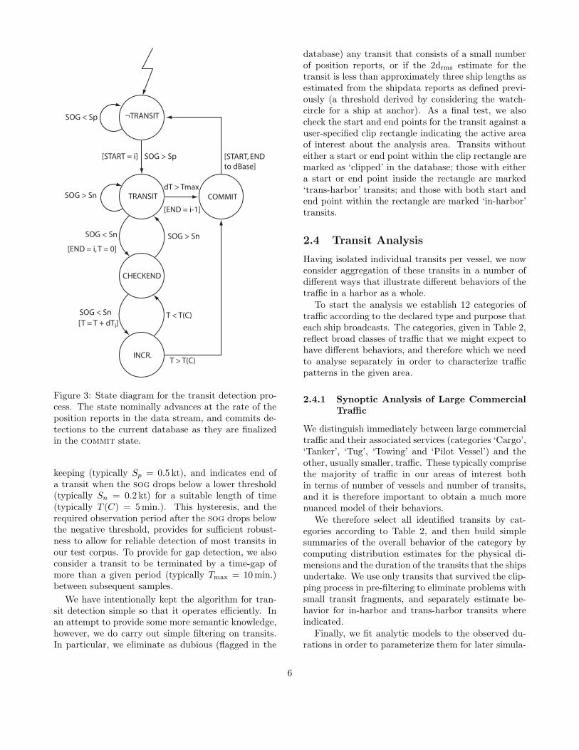
We therefore construct transits by considering thespeed over ground (sog) estimate distributed in theais messages, which benefits from the smoothing ofthe Kalman filter implemented in the gps providingthe information to the ais transceiver. In order to sat-isfy the conditions laid out above, we implement thedetection algorithm as a simple synchronous state ma-chine as illustrated in Figure 3. The algorithm startsto indicate a transit when the sog rises above station

5

¬TRANSIT

TRANSIT

CHECKEND

INCR.

COMMIT

SOG < Sp

SOG > Sp

SOG > Sn

SOG < Sn SOG > Sn

[END = i, T = 0]

T < T(C)SOG < Sn

[T = T + dTi]

T > T(C)

[END = i-1]

dT > Tmax

[START, END

to dBase]

[START = i]

Figure 3: State diagram for the transit detection pro-cess. The state nominally advances at the rate of theposition reports in the data stream, and commits de-tections to the current database as they are finalizedin the commit state.

keeping (typically Sp = 0.5 kt), and indicates end ofa transit when the sog drops below a lower threshold(typically Sn = 0.2 kt) for a suitable length of time(typically T (C) = 5 min.). This hysteresis, and therequired observation period after the sog drops belowthe negative threshold, provides for sufficient robust-ness to allow for reliable detection of most transits inour test corpus. To provide for gap detection, we alsoconsider a transit to be terminated by a time-gap ofmore than a given period (typically Tmax = 10 min.)between subsequent samples.

We have intentionally kept the algorithm for tran-sit detection simple so that it operates efficiently. Inan attempt to provide some more semantic knowledge,however, we do carry out simple filtering on transits.In particular, we eliminate as dubious (flagged in the

database) any transit that consists of a small numberof position reports, or if the 2drms estimate for thetransit is less than approximately three ship lengths asestimated from the shipdata reports as defined previ-ously (a threshold derived by considering the watch-circle for a ship at anchor). As a final test, we alsocheck the start and end points for the transit against auser-specified clip rectangle indicating the active areaof interest about the analysis area. Transits withouteither a start or end point within the clip rectangle aremarked as ‘clipped’ in the database; those with eithera start or end point inside the rectangle are marked‘trans-harbor’ transits; and those with both start andend point within the rectangle are marked ‘in-harbor’transits.

2.4 Transit Analysis

Having isolated individual transits per vessel, we nowconsider aggregation of these transits in a number ofdifferent ways that illustrate different behaviors of thetraffic in a harbor as a whole.

To start the analysis we establish 12 categories oftraffic according to the declared type and purpose thateach ship broadcasts. The categories, given in Table 2,reflect broad classes of traffic that we might expect tohave different behaviors, and therefore which we needto analyse separately in order to characterize trafficpatterns in the given area.

2.4.1 Synoptic Analysis of Large CommercialTraffic

We distinguish immediately between large commercialtraffic and their associated services (categories ‘Cargo’,‘Tanker’, ‘Tug’, ‘Towing’ and ‘Pilot Vessel’) and theother, usually smaller, traffic. These typically comprisethe majority of traffic in our areas of interest bothin terms of number of vessels and number of transits,and it is therefore important to obtain a much morenuanced model of their behaviors.

We therefore select all identified transits by cat-egories according to Table 2, and then build simplesummaries of the overall behavior of the category bycomputing distribution estimates for the physical di-mensions and the duration of the transits that the shipsundertake. We use only transits that survived the clip-ping process in pre-filtering to eliminate problems withsmall transit fragments, and separately estimate be-havior for in-harbor and trans-harbor transits whereindicated.

Finally, we fit analytic models to the observed du-rations in order to parameterize them for later simula-

6

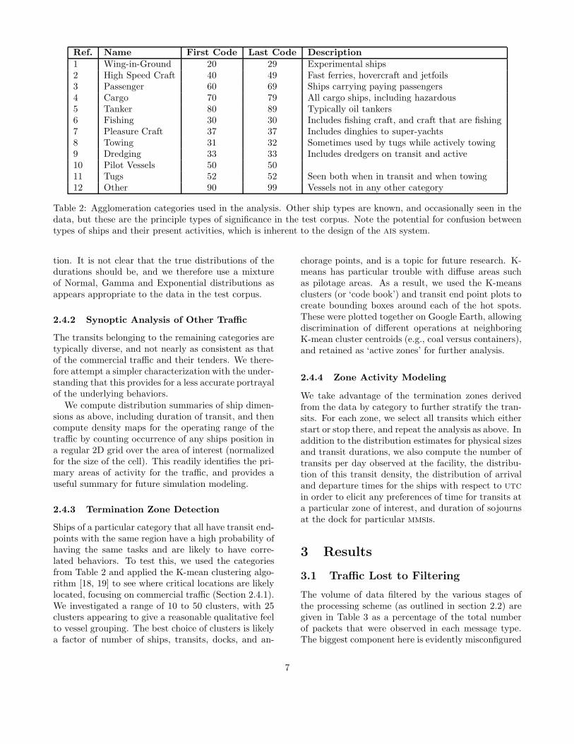
Ref. Name First Code Last Code Description1 Wing-in-Ground 20 29 Experimental ships2 High Speed Craft 40 49 Fast ferries, hovercraft and jetfoils3 Passenger 60 69 Ships carrying paying passengers4 Cargo 70 79 All cargo ships, including hazardous5 Tanker 80 89 Typically oil tankers6 Fishing 30 30 Includes fishing craft, and craft that are fishing7 Pleasure Craft 37 37 Includes dinghies to super-yachts8 Towing 31 32 Sometimes used by tugs while actively towing9 Dredging 33 33 Includes dredgers on transit and active10 Pilot Vessels 50 5011 Tugs 52 52 Seen both when in transit and when towing12 Other 90 99 Vessels not in any other category

Table 2: Agglomeration categories used in the analysis. Other ship types are known, and occasionally seen in thedata, but these are the principle types of significance in the test corpus. Note the potential for confusion betweentypes of ships and their present activities, which is inherent to the design of the ais system.

tion. It is not clear that the true distributions of thedurations should be, and we therefore use a mixtureof Normal, Gamma and Exponential distributions asappears appropriate to the data in the test corpus.

2.4.2 Synoptic Analysis of Other Traffic

The transits belonging to the remaining categories aretypically diverse, and not nearly as consistent as thatof the commercial traffic and their tenders. We there-fore attempt a simpler characterization with the under-standing that this provides for a less accurate portrayalof the underlying behaviors.

We compute distribution summaries of ship dimen-sions as above, including duration of transit, and thencompute density maps for the operating range of thetraffic by counting occurrence of any ships position ina regular 2D grid over the area of interest (normalizedfor the size of the cell). This readily identifies the pri-mary areas of activity for the traffic, and provides auseful summary for future simulation modeling.

2.4.3 Termination Zone Detection

Ships of a particular category that all have transit end-points with the same region have a high probability ofhaving the same tasks and are likely to have corre-lated behaviors. To test this, we used the categoriesfrom Table 2 and applied the K-mean clustering algo-rithm [18, 19] to see where critical locations are likelylocated, focusing on commercial traffic (Section 2.4.1).We investigated a range of 10 to 50 clusters, with 25clusters appearing to give a reasonable qualitative feelto vessel grouping. The best choice of clusters is likelya factor of number of ships, transits, docks, and an-

chorage points, and is a topic for future research. K-means has particular trouble with diffuse areas suchas pilotage areas. As a result, we used the K-meansclusters (or ‘code book’) and transit end point plots tocreate bounding boxes around each of the hot spots.These were plotted together on Google Earth, allowingdiscrimination of different operations at neighboringK-mean cluster centroids (e.g., coal versus containers),and retained as ‘active zones’ for further analysis.

2.4.4 Zone Activity Modeling

We take advantage of the termination zones derivedfrom the data by category to further stratify the tran-sits. For each zone, we select all transits which eitherstart or stop there, and repeat the analysis as above. Inaddition to the distribution estimates for physical sizesand transit durations, we also compute the number oftransits per day observed at the facility, the distribu-tion of this transit density, the distribution of arrivaland departure times for the ships with respect to utcin order to elicit any preferences of time for transits ata particular zone of interest, and duration of sojournsat the dock for particular mmsis.

3 Results

3.1 Traffic Lost to Filtering

The volume of data filtered by the various stages ofthe processing scheme (as outlined in section 2.2) aregiven in Table 3 as a percentage of the total numberof packets that were observed in each message type.The biggest component here is evidently misconfigured

7

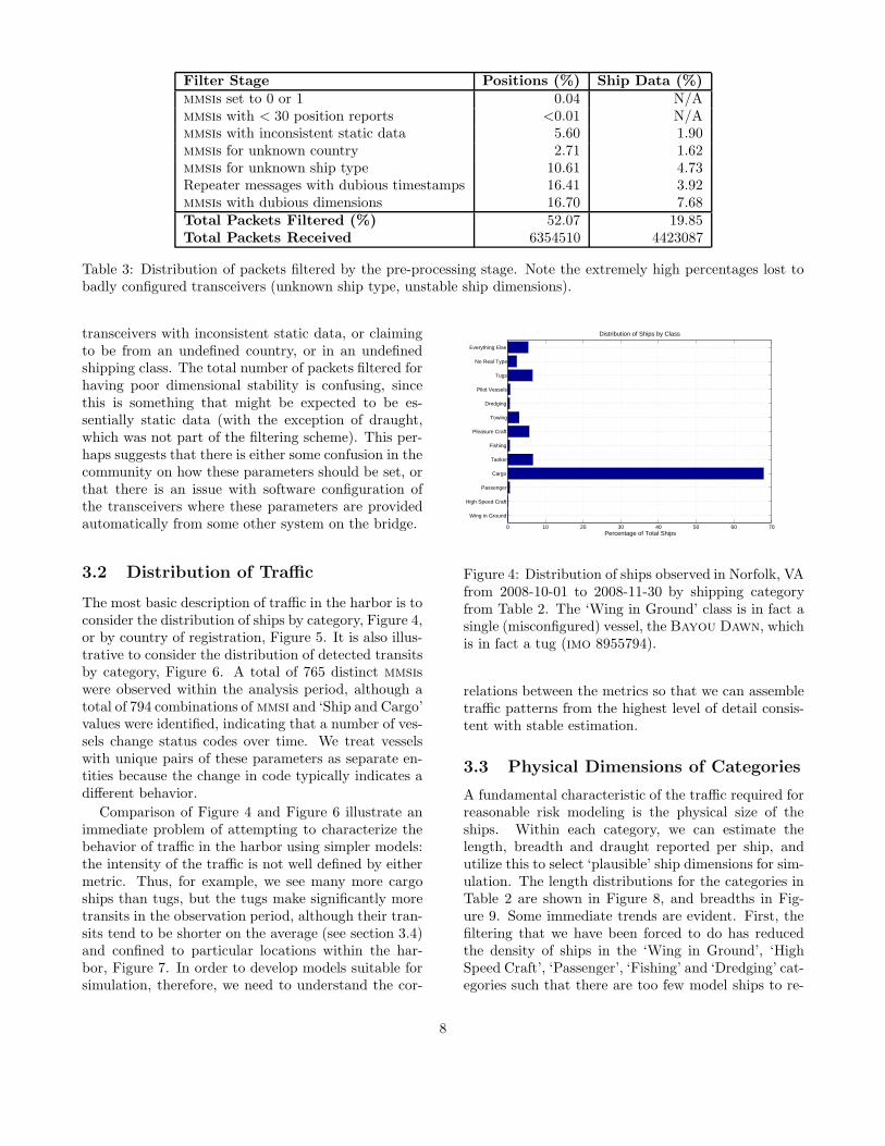
Filter Stage Positions (%) Ship Data (%)mmsis set to 0 or 1 0.04 N/Ammsis with < 30 position reports <0.01 N/Ammsis with inconsistent static data 5.60 1.90mmsis for unknown country 2.71 1.62mmsis for unknown ship type 10.61 4.73Repeater messages with dubious timestamps 16.41 3.92mmsis with dubious dimensions 16.70 7.68Total Packets Filtered (%) 52.07 19.85Total Packets Received 6354510 4423087

Table 3: Distribution of packets filtered by the pre-processing stage. Note the extremely high percentages lost tobadly configured transceivers (unknown ship type, unstable ship dimensions).

transceivers with inconsistent static data, or claimingto be from an undefined country, or in an undefinedshipping class. The total number of packets filtered forhaving poor dimensional stability is confusing, sincethis is something that might be expected to be es-sentially static data (with the exception of draught,which was not part of the filtering scheme). This per-haps suggests that there is either some confusion in thecommunity on how these parameters should be set, orthat there is an issue with software configuration ofthe transceivers where these parameters are providedautomatically from some other system on the bridge.

3.2 Distribution of Traffic

The most basic description of traffic in the harbor is toconsider the distribution of ships by category, Figure 4,or by country of registration, Figure 5. It is also illus-trative to consider the distribution of detected transitsby category, Figure 6. A total of 765 distinct mmsiswere observed within the analysis period, although atotal of 794 combinations of mmsi and ‘Ship and Cargo’values were identified, indicating that a number of ves-sels change status codes over time. We treat vesselswith unique pairs of these parameters as separate en-tities because the change in code typically indicates adifferent behavior.

Comparison of Figure 4 and Figure 6 illustrate animmediate problem of attempting to characterize thebehavior of traffic in the harbor using simpler models:the intensity of the traffic is not well defined by eithermetric. Thus, for example, we see many more cargoships than tugs, but the tugs make significantly moretransits in the observation period, although their tran-sits tend to be shorter on the average (see section 3.4)and confined to particular locations within the har-bor, Figure 7. In order to develop models suitable forsimulation, therefore, we need to understand the cor-

0 10 20 30 40 50 60 70

Wing in Ground

High Speed Craft

Passenger

Cargo

Tanker

Fishing

Pleasure Craft

Towing

Dredging

Pilot Vessels

Tugs

No Real Type

Everything Else

Percentage of Total Ships

Distribution of Ships by Class

Figure 4: Distribution of ships observed in Norfolk, VAfrom 2008-10-01 to 2008-11-30 by shipping categoryfrom Table 2. The ‘Wing in Ground’ class is in fact asingle (misconfigured) vessel, the Bayou Dawn, whichis in fact a tug (imo 8955794).

relations between the metrics so that we can assembletraffic patterns from the highest level of detail consis-tent with stable estimation.

3.3 Physical Dimensions of Categories

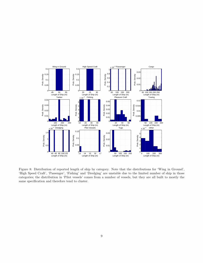
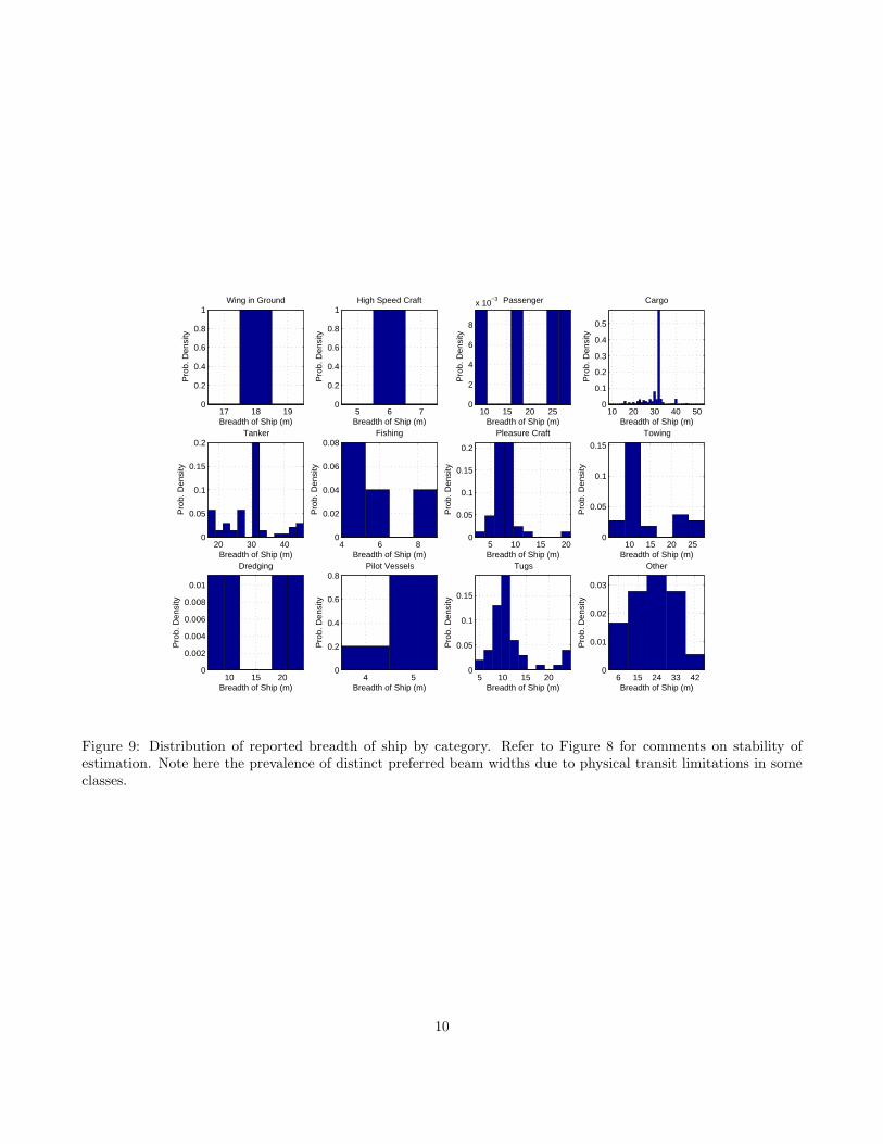
A fundamental characteristic of the traffic required forreasonable risk modeling is the physical size of theships. Within each category, we can estimate thelength, breadth and draught reported per ship, andutilize this to select ‘plausible’ ship dimensions for sim-ulation. The length distributions for the categories inTable 2 are shown in Figure 8, and breadths in Fig-ure 9. Some immediate trends are evident. First, thefiltering that we have been forced to do has reducedthe density of ships in the ‘Wing in Ground’, ‘HighSpeed Craft’, ‘Passenger’, ‘Fishing’ and ‘Dredging’ cat-egories such that there are too few model ships to re-

8

45 50 550

0.05

0.1

0.15

0.2

Length of Ship (m)

Pro

b. D

ensi

ty

Wing in Ground

20 25 300

0.05

0.1

0.15

0.2

Length of Ship (m)

Pro

b. D

ensi

ty

High Speed Craft

50 100 150 2000

0.2

0.4

0.6

0.8

1x 10

−3

Length of Ship (m)

Pro

b. D

ensi

ty

Passenger

50 100 150 200 2500

0.01

0.02

0.03

Length of Ship (m)

Pro

b. D

ensi

ty

Cargo

150 200 2500

0.01

0.02

0.03

0.04

Length of Ship (m)

Pro

b. D

ensi

ty

Tanker

10 20 30 400

1

2

3

4

5

x 10−3

Length of Ship (m)

Pro

b. D

ensi

ty

Fishing

20 40 600

0.01

0.02

0.03

0.04

0.05

Length of Ship (m)

Pro

b. D

ensi

ty

Pleasure Craft

50 100 150 2000

0.005

0.01

0.015

0.02

Length of Ship (m)

Pro

b. D

ensi

ty

Towing

40 60 80 1001200

0.5

1

1.5

x 10−3

Length of Ship (m)

Pro

b. D

ensi

ty

Dredging

13 14 15 16 170

0.05

0.1

0.15

Length of Ship (m)

Pro

b. D

ensi

ty

Pilot Vessels

50 100 150 2000

0.01

0.02

0.03

Length of Ship (m)

Pro

b. D

ensi

ty

Tugs

0 100 200 3000

1

2

3

4

5

x 10−3

Length of Ship (m)

Pro

b. D

ensi

ty

Other

Figure 8: Distribution of reported length of ship by category. Note that the distributions for ‘Wing in Ground’,‘High Speed Craft’, ‘Passenger’, ‘Fishing’ and ‘Dredging’ are unstable due to the limited number of ship in thosecategories; the distribution in ‘Pilot vessels’ comes from a number of vessels, but they are all built to mostly thesame specification and therefore tend to cluster.

9

17 18 190

0.2

0.4

0.6

0.8

1

Breadth of Ship (m)

Pro

b. D

ensi

ty

Wing in Ground

5 6 70

0.2

0.4

0.6

0.8

1

Breadth of Ship (m)

Pro

b. D

ensi

ty

High Speed Craft

10 15 20 250

2

4

6

8

x 10−3

Breadth of Ship (m)

Pro

b. D

ensi

ty

Passenger

10 20 30 40 500

0.1

0.2

0.3

0.4

0.5

Breadth of Ship (m)

Pro

b. D

ensi

ty

Cargo

20 30 400

0.05

0.1

0.15

0.2

Breadth of Ship (m)

Pro

b. D

ensi

ty

Tanker

4 6 80

0.02

0.04

0.06

0.08

Breadth of Ship (m)

Pro

b. D

ensi

ty

Fishing

5 10 15 200

0.05

0.1

0.15

0.2

Breadth of Ship (m)

Pro

b. D

ensi

ty

Pleasure Craft

10 15 20 250

0.05

0.1

0.15

Breadth of Ship (m)

Pro

b. D

ensi

ty

Towing

10 15 200

0.002

0.004

0.006

0.008

0.01

Breadth of Ship (m)

Pro

b. D

ensi

ty

Dredging

4 50

0.2

0.4

0.6

0.8

Breadth of Ship (m)

Pro

b. D

ensi

ty

Pilot Vessels

5 10 15 200

0.05

0.1

0.15

Breadth of Ship (m)

Pro

b. D

ensi

ty

Tugs

6 15 24 33 420

0.01

0.02

0.03

Breadth of Ship (m)

Pro

b. D

ensi

ty

Other

Figure 9: Distribution of reported breadth of ship by category. Refer to Figure 8 for comments on stability ofestimation. Note here the prevalence of distinct preferred beam widths due to physical transit limitations in someclasses.

10

0 5 10 15 20 25

United States

Panama

Liberia

Marshall Islands

Hong Kong

Bahamas

Singapore

Germany

United Kingdom

Malta

Everywhere Else

Percentage of Total Ships

Distribution of Ships by Country of Registration

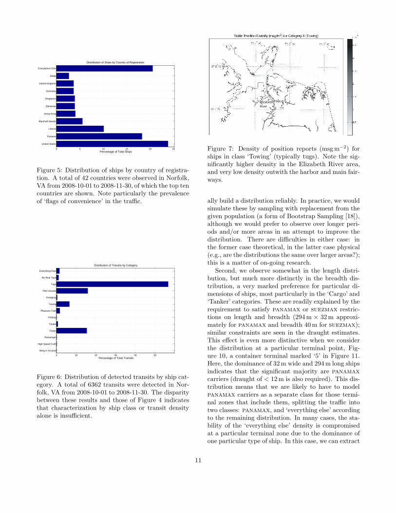
Figure 5: Distribution of ships by country of registra-tion. A total of 42 countries were observed in Norfolk,VA from 2008-10-01 to 2008-11-30, of which the top tencountries are shown. Note particularly the prevalenceof ‘flags of convenience’ in the traffic.

0 10 20 30 40 50

Wing in Ground

High Speed Craft

Passenger

Cargo

Tanker

Fishing

Pleasure Craft

Towing

Dredging

Pilot Vessels

Tugs

No Real Type

Everything Else

Percentage of Total Transits

Distribution of Transits by Category

Figure 6: Distribution of detected transits by ship cat-egory. A total of 6362 transits were detected in Nor-folk, VA from 2008-10-01 to 2008-11-30. The disparitybetween these results and those of Figure 4 indicatesthat characterization by ship class or transit densityalone is insufficient.

Elizabeth

River

Figure 7: Density of position reports (msg m−2) forships in class ‘Towing’ (typically tugs). Note the sig-nificantly higher density in the Elizabeth River area,and very low density outwith the harbor and main fair-ways.

ally build a distribution reliably. In practice, we wouldsimulate these by sampling with replacement from thegiven population (a form of Bootstrap Sampling [18]),although we would prefer to observe over longer peri-ods and/or more areas in an attempt to improve thedistribution. There are difficulties in either case: inthe former case theoretical, in the latter case physical(e.g., are the distributions the same over larger areas?);this is a matter of on-going research.

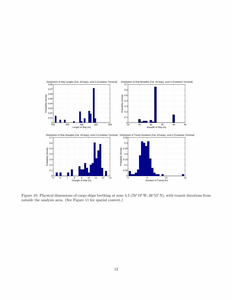
Second, we observe somewhat in the length distri-bution, but much more distinctly in the breadth dis-tribution, a very marked preference for particular di-mensions of ships, most particularly in the ‘Cargo’ and‘Tanker’ categories. These are readily explained by therequirement to satisfy panamax or suezmax restric-tions on length and breadth (294 m × 32 m approxi-mately for panamax and breadth 40 m for suezmax);similar constraints are seen in the draught estimates.This effect is even more distinctive when we considerthe distribution at a particular terminal point, Fig-ure 10, a container terminal marked ‘5’ in Figure 11.Here, the dominance of 32 m wide and 294 m long shipsindicates that the significant majority are panamaxcarriers (draught of < 12 m is also required). This dis-tribution means that we are likely to have to modelpanamax carriers as a separate class for those termi-nal zones that include them, splitting the traffic intotwo classes: panamax, and ‘everything else’ accordingto the remaining distribution. In many cases, the sta-bility of the ‘everything else’ density is compromisedat a particular terminal zone due to the dominance ofone particular type of ship. In this case, we can extract

11

150 200 250 300 3500

0.01

0.02

0.03

0.04

0.05

0.06

0.07

0.08

Length of Ship (m)

Pro

babi

lity

Den

sity

Distribution of Ship Lengths (Cat. 4/Cargo), zone 5 (Container Terminal)

20 25 30 35 40 450

0.1

0.2

0.3

0.4

0.5

0.6

0.7

Breadth of Ship (m)

Pro

babi

lity

Den

sity

Distribution of Ship Breadths (Cat. 4/Cargo), zone 5 (Container Terminal)

5 6 7 8 9 10 11 12 130

0.1

0.2

0.3

0.4

0.5

0.6

0.7

Draught of Ship (m)

Pro

babi

lity

Den

sity

Distribution of Ship Draughts (Cat. 4/Cargo), zone 5 (Container Terminal)

0 5 10 150

0.05

0.1

0.15

0.2

0.25

0.3

0.35

Duration of Transit (hr)

Pro

babi

lity

Den

sity

Distribution of Transit Durations (Cat. 4/Cargo), zone 5 (Container Terminal)

Figure 10: Physical dimensions of cargo ships berthing at zone 4.5 (76◦19′ W, 36◦55′ N), with transit durations fromoutside the analysis area. (See Figure 11 for spatial context.)

12

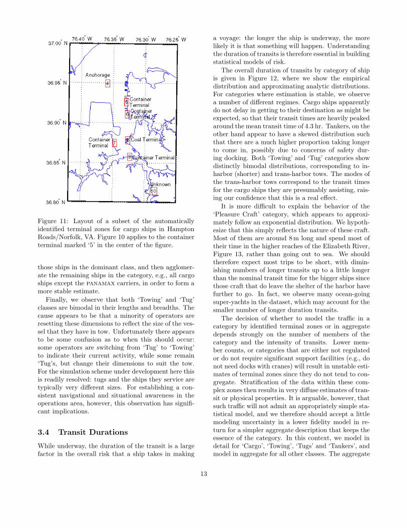
Figure 11: Layout of a subset of the automaticallyidentified terminal zones for cargo ships in HamptonRoads/Norfolk, VA. Figure 10 applies to the containerterminal marked ‘5’ in the center of the figure.

those ships in the dominant class, and then agglomer-ate the remaining ships in the category, e.g., all cargoships except the panamax carriers, in order to form amore stable estimate.

Finally, we observe that both ‘Towing’ and ‘Tug’classes are bimodal in their lengths and breadths. Thecause appears to be that a minority of operators areresetting these dimensions to reflect the size of the ves-sel that they have in tow. Unfortunately there appearsto be some confusion as to when this should occur:some operators are switching from ‘Tug’ to ‘Towing’to indicate their current activity, while some remain‘Tug’s, but change their dimensions to suit the tow.For the simulation scheme under development here thisis readily resolved: tugs and the ships they service aretypically very different sizes. For establishing a con-sistent navigational and situational awareness in theoperations area, however, this observation has signifi-cant implications.

3.4 Transit Durations

While underway, the duration of the transit is a largefactor in the overall risk that a ship takes in making

a voyage: the longer the ship is underway, the morelikely it is that something will happen. Understandingthe duration of transits is therefore essential in buildingstatistical models of risk.

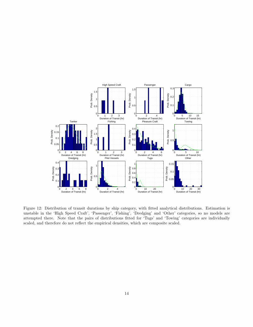
The overall duration of transits by category of shipis given in Figure 12, where we show the empiricaldistribution and approximating analytic distributions.For categories where estimation is stable, we observea number of different regimes. Cargo ships apparentlydo not delay in getting to their destination as might beexpected, so that their transit times are heavily peakedaround the mean transit time of 4.3 hr. Tankers, on theother hand appear to have a skewed distribution suchthat there are a much higher proportion taking longerto come in, possibly due to concerns of safety dur-ing docking. Both ‘Towing’ and ‘Tug’ categories showdistinctly bimodal distributions, corresponding to in-harbor (shorter) and trans-harbor tows. The modes ofthe trans-harbor tows correspond to the transit timesfor the cargo ships they are presumably assisting, rais-ing our confidence that this is a real effect.

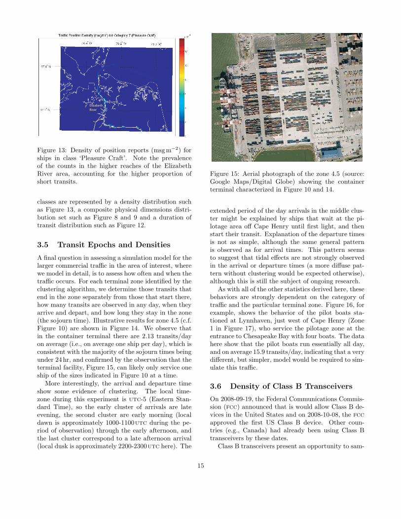
It is more difficult to explain the behavior of the‘Pleasure Craft’ category, which appears to approxi-mately follow an exponential distribution. We hypoth-esize that this simply reflects the nature of these craft.Most of them are around 8m long and spend most oftheir time in the higher reaches of the Elizabeth River,Figure 13, rather than going out to sea. We shouldtherefore expect most trips to be short, with dimin-ishing numbers of longer transits up to a little longerthan the nominal transit time for the bigger ships sincethose craft that do leave the shelter of the harbor havefurther to go. In fact, we observe many ocean-goingsuper-yachts in the dataset, which may account for thesmaller number of longer duration transits.

The decision of whether to model the traffic in acategory by identified terminal zones or in aggregatedepends strongly on the number of members of thecategory and the intensity of transits. Lower mem-ber counts, or categories that are either not regulatedor do not require significant support facilities (e.g., donot need docks with cranes) will result in unstable esti-mates of terminal zones since they do not tend to con-gregate. Stratification of the data within these com-plex zones then results in very diffuse estimates of tran-sit or physical properties. It is arguable, however, thatsuch traffic will not admit an appropriately simple sta-tistical model, and we therefore should accept a littlemodeling uncertainty in a lower fidelity model in re-turn for a simpler aggregate description that keeps theessence of the category. In this context, we model indetail for ‘Cargo’, ‘Towing’, ‘Tugs’ and ‘Tankers’, andmodel in aggregate for all other classes. The aggregate

13

0 1 2 30

0.5

1

1.5

Duration of Transit (hr)

Pro

b. D

ensi

ty

High Speed Craft

0 2 40

0.5

1

1.5

Duration of Transit (hr)

Pro

b. D

ensi

ty

Passenger

0 5 10 150

0.1

0.2

0.3

Duration of Transit (hr)

Pro

b. D

ensi

ty

Cargo

0 2 4 6 80

0.05

0.1

0.15

0.2

Duration of Transit (hr)

Pro

b. D

ensi

ty

Tanker

0 1 2 30

0.5

1

1.5

2

Duration of Transit (hr)

Pro

b. D

ensi

ty

Fishing

0 2 4 60

0.1

0.2

0.3

0.4

Duration of Transit (hr)

Pro

b. D

ensi

ty

Pleasure Craft

0 5 100

0.5

1

Duration of Transit (hr)

Pro

b. D

ensi

ty

Towing

0 2 4 6 80

0.1

0.2

0.3

0.4

Duration of Transit (hr)

Pro

b. D

ensi

ty

Dredging

0 2 40

0.5

1

Duration of Transit (hr)

Pro

b. D

ensi

ty

Pilot Vessels

0 10 200

0.2

0.4

0.6

0.8

1

Duration of Transit (hr)

Pro

b. D

ensi

ty

Tugs

0 10 20 300

0.05

0.1

0.15

Duration of Transit (hr)

Pro

b. D

ensi

ty

Other

Figure 12: Distribution of transit durations by ship category, with fitted analytical distributions. Estimation isunstable in the ‘High Speed Craft’, ‘Passenger’, ‘Fishing’, ‘Dredging’ and ‘Other’ categories, so no models areattempted there. Note that the pairs of distributions fitted for ‘Tugs’ and ‘Towing’ categories are individuallyscaled, and therefore do not reflect the empirical densities, which are composite scaled.

14

Elizabeth

River

Figure 13: Density of position reports (msgm−2) forships in class ‘Pleasure Craft’. Note the prevalenceof the counts in the higher reaches of the ElizabethRiver area, accounting for the higher proportion ofshort transits.

classes are represented by a density distribution suchas Figure 13, a composite physical dimensions distri-bution set such as Figure 8 and 9 and a duration oftransit distribution such as Figure 12.

3.5 Transit Epochs and Densities

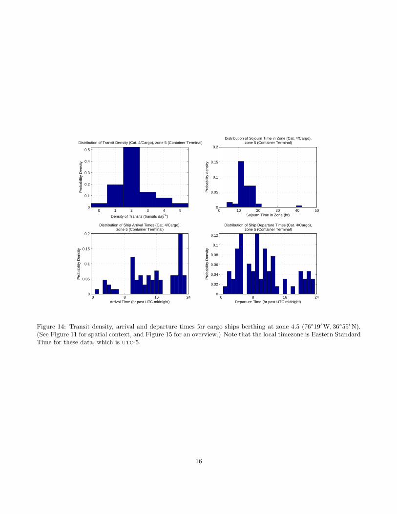
A final question in assessing a simulation model for thelarger commercial traffic in the area of interest, wherewe model in detail, is to assess how often and when thetraffic occurs. For each terminal zone identified by theclustering algorithm, we determine those transits thatend in the zone separately from those that start there,how many transits are observed in any day, when theyarrive and depart, and how long they stay in the zone(the sojourn time). Illustrative results for zone 4.5 (c.f.Figure 10) are shown in Figure 14. We observe thatin the container terminal there are 2.13 transits/dayon average (i.e., on average one ship per day), which isconsistent with the majority of the sojourn times beingunder 24hr, and confirmed by the observation that theterminal facility, Figure 15, can likely only service oneship of the sizes indicated in Figure 10 at a time.

More interestingly, the arrival and departure timeshow some evidence of clustering. The local time-zone during this experiment is utc-5 (Eastern Stan-dard Time), so the early cluster of arrivals are lateevening, the second cluster are early morning (localdawn is approximately 1000-1100utc during the pe-riod of observation) through the early afternoon, andthe last cluster correspond to a late afternoon arrival(local dusk is approximately 2200-2300utc here). The

Figure 15: Aerial photograph of the zone 4.5 (source:Google Maps/Digital Globe) showing the containerterminal characterized in Figure 10 and 14.

extended period of the day arrivals in the middle clus-ter might be explained by ships that wait at the pi-lotage area off Cape Henry until first light, and thenstart their transit. Explanation of the departure timesis not as simple, although the same general patternis observed as for arrival times. This pattern seemsto suggest that tidal effects are not strongly observedin the arrival or departure times (a more diffuse pat-tern without clustering would be expected otherwise),although this is still the subject of ongoing research.

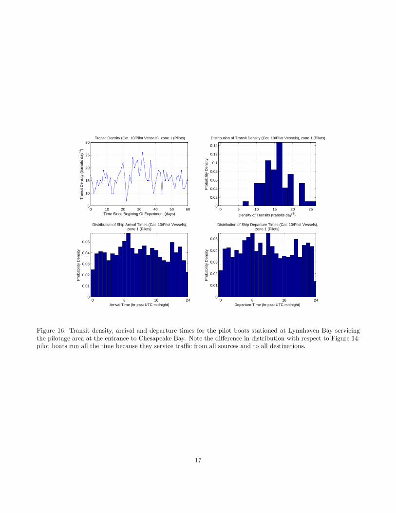
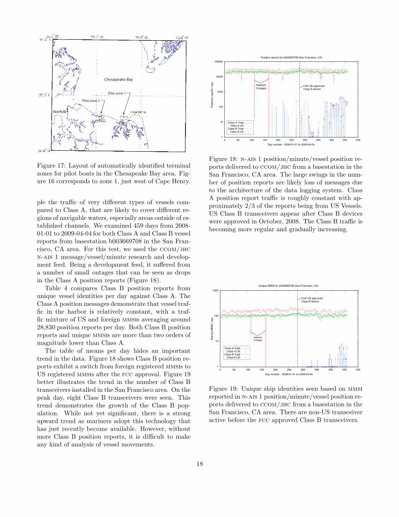
As with all of the other statistics derived here, thesebehaviors are strongly dependent on the category oftraffic and the particular terminal zone. Figure 16, forexample, shows the behavior of the pilot boats sta-tioned at Lynnhaven, just west of Cape Henry (Zone1 in Figure 17), who service the pilotage zone at theentrance to Chesapeake Bay with four boats. The datahere show that the pilot boats run essentially all day,and on average 15.9 transits/day, indicating that a verydifferent, but simpler, model would be required to sim-ulate this traffic.

3.6 Density of Class B Transceivers

On 2008-09-19, the Federal Communications Commis-sion (fcc) announced that is would allow Class B de-vices in the United States and on 2008-10-08, the fccapproved the first US Class B device. Other coun-tries (e.g., Canada) had already been using Class Btransceivers by these dates.

Class B transceivers present an opportunity to sam-

15

0 1 2 3 4 50

0.1

0.2

0.3

0.4

0.5

Density of Transits (transits day−1)

Pro

babi

lity

Den

sity

Distribution of Transit Density (Cat. 4/Cargo), zone 5 (Container Terminal)

0 10 20 30 40 500

0.05

0.1

0.15

0.2

Sojourn Time in Zone (hr)

Pro

babi

lity

dens

ity

Distribution of Sojourn Time in Zone (Cat. 4/Cargo),zone 5 (Container Terminal)

0 8 16 240

0.05

0.1

0.15

0.2

Arrival Time (hr past UTC midnight)

Pro

babi

lity

Den

sity

Distribution of Ship Arrival Times (Cat. 4/Cargo),zone 5 (Container Terminal)

0 8 16 240

0.02

0.04

0.06

0.08

0.1

0.12

Departure Time (hr past UTC midnight)

Pro

babi

lity

Den

sity

Distribution of Ship Departure Times (Cat. 4/Cargo),zone 5 (Container Terminal)

Figure 14: Transit density, arrival and departure times for cargo ships berthing at zone 4.5 (76◦19′ W, 36◦55′ N).(See Figure 11 for spatial context, and Figure 15 for an overview.) Note that the local timezone is Eastern StandardTime for these data, which is utc-5.

16

0 10 20 30 40 50 605

10

15

20

25

30

Time Since Begining Of Experiment (days)

Tra

nsit

Den

sity

(tr

ansi

ts d

ay−

1 )

Transit Density (Cat. 10/Pilot Vessels), zone 1 (Pilots)

0 5 10 15 20 250

0.02

0.04

0.06

0.08

0.1

0.12

0.14

Density of Transits (transits day−1)

Pro

babi

lity

Den

sity

Distribution of Transit Density (Cat. 10/Pilot Vessels), zone 1 (Pilots)

0 8 16 240

0.01

0.02

0.03

0.04

0.05

Arrival Time (hr past UTC midnight)

Pro

babi

lity

Den

sity

Distribution of Ship Arrival Times (Cat. 10/Pilot Vessels),zone 1 (Pilots)

0 8 16 240

0.01

0.02

0.03

0.04

0.05

Departure Time (hr past UTC midnight)

Pro

babi

lity

Den

sity

Distribution of Ship Departure Times (Cat. 10/Pilot Vessels),zone 1 (Pilots)

Figure 16: Transit density, arrival and departure times for the pilot boats stationed at Lynnhaven Bay servicingthe pilotage area at the entrance to Chesapeake Bay. Note the difference in distribution with respect to Figure 14:pilot boats run all the time because they service traffic from all sources and to all destinations.

17

Chesapeake Bay

Norfolk

Pilot zone 1

Pilot zone 2

Figure 17: Layout of automatically identified terminalzones for pilot boats in the Chesapeake Bay area. Fig-ure 16 corresponds to zone 1, just west of Cape Henry.

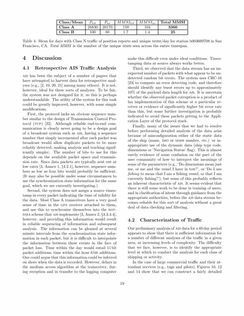
ple the traffic of very different types of vessels com-pared to Class A, that are likely to cover different re-gions of navigable waters, especially areas outside of es-tablished channels. We examined 459 days from 2008-01-01 to 2009-04-04 for both Class A and Class B vesselreports from basestation b003669708 in the San Fran-cisco, CA area. For this test, we used the ccom/jhcn-ais 1 message/vessel/minute research and develop-ment feed. Being a development feed, it suffered froma number of small outages that can be seen as dropsin the Class A position reports (Figure 18).

Table 4 compares Class B position reports fromunique vessel identities per day against Class A. TheClass A position messages demonstrate that vessel traf-fic in the harbor is relatively constant, with a traf-fic mixture of US and foreign mmsis averaging around28,830 position reports per day. Both Class B positionreports and unique mmsis are more than two orders ofmagnitude lower than Class A.

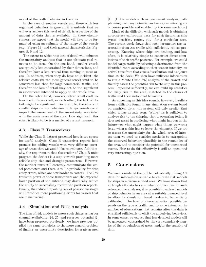
The table of means per day hides an importanttrend in the data. Figure 18 shows Class B position re-ports exhibit a switch from foreign registered mmsis toUS registered mmsis after the fcc approval. Figure 19better illustrates the trend in the number of Class Btransceivers installed in the San Francisco area. On thepeak day, eight Class B transceivers were seen. Thistrend demonstrates the growth of the Class B pop-ulation. While not yet significant, there is a strongupward trend as mariners adopt this technology thathas just recently become available. However, withoutmore Class B position reports, it is difficult to makeany kind of analysis of vessel movements.

1

10

100

1000

10000

100000

0 50 100 150 200 250 300 350 400 450 500

Po

sitio

ns r

ep

ort

s / d

ay

Day number - 2008-01-01 to 2009-04-04

Position reports for b003669708 (San Francisco, CA)

Network

Outages

Class A TotalClass A US

Class B TotalClass B US

First US approved

Class B device

Figure 18: n-ais 1 position/minute/vessel position re-ports delivered to ccom/jhc from a basestation in theSan Francisco, CA area. The large swings in the num-ber of position reports are likely loss of messages dueto the architecture of the data logging system. ClassA position report traffic is roughly constant with ap-proximately 2/3 of the reports being from US Vessels.US Class B transceivers appear after Class B deviceswere approved in October, 2008. The Class B traffic isbecoming more regular and gradually increasing.

1

10

100

1000

0 50 100 150 200 250 300 350 400 450 500

Dis

tin

ct M

MS

I / d

ay

Day number - 2008-01-01 to 2009-04-04

Unique MMSI for b003669708 (San Francisco, CA)

Class A TotalClass A US

Class B TotalClass B US

Network

Outages

First US approved

Class B device

Figure 19: Unique ship identities seen based on mmsireported in n-ais 1 position/minute/vessel position re-ports delivered to ccom/jhc from a basestation in theSan Francisco, CA area. There are non-US transceiveractive before the fcc approved Class B transceivers.

18

Class/Mean Ptot Pus MMSItot MMSIus Total MMSIClass A 28830 20170 159 104 3366Class B 100 80 1.7 1.4 25

Table 4: Mean for days with Class N traffic of position reports and unique mmsi/day for station b003669708 in SanFrancisco, CA. Total MMSI is the number of the unique mmsi seen across the entire timespan.

4 Discussion

4.1 Retrospective AIS Traffic Analysis

ais has been the subject of a number of papers thathave attempted to harvest data for retrospective anal-yses (e.g., [2, 10, 20, 21] among many others). It is not,however, ideal for these sorts of analyses. To be fair,the system was not designed for it, so this is perhapsunderstandable. The utility of the system for this taskcould be greatly improved, however, with some simplemodifications.

First, the protocol lacks an obvious sequence num-ber similar to the design of Transmission Control Pro-tocol (tcp) [22]. Although reliable end-to-end com-munication is clearly never going to be a design goalof a broadcast system such as ais, having a sequencenumber that simply incremented after each packet wasbroadcast would allow duplicate packets to be morereliably detected, making analysis and tracking signif-icantly simpler. The number of bits to use for thisdepends on the available packet space and transmis-sion rate. Since data packets are typically sent out atlow rates [3, Annex 1, §4.2.1], however, sequence num-bers as low as four bits would probably be sufficient.(It may also be possible under some circumstances touse the synchronization state information for the samegoal, which we are currently investigating.)

Second, the system does not assign a source times-tamp in every packet indicating the time of validity forthe data. Most Class A transceivers have a very goodsense of time in the gps receiver attached to them,and use this to synchronize themselves into the sot-dma scheme that ais implements [3, Annex 2, §3.3.4.4],however, and providing this information would resultin reliable sequencing of information and subsequentanalysis. The information can be gleaned at severalminute intervals from the synchronization state infor-mation in each packet, but it is difficult to interpolatethe information between these events in the face ofpacket loss. Time within the day would entail 11bitpacket additions; time within the hour 6 bit additions.One could argue that this information could be inferredon shore when the data is recorded. However, delays inthe medium access algorithm at the transceiver, dur-ing reception and in transfer to the logging computer

make this difficult even under ideal conditions. Times-tamping data at source always works better.

Third, we observed that the data stream has an un-expected number of packets with what appear to be un-detected random bit errors. The system uses CRC-16[23] to compute an error detecting code, and thereforeshould identify any burst errors up to approximately10% of the payload data length for ais. It is uncertainwhether the observed packet corruption is a product oflax implementation of this scheme at a particular re-ceiver or evidence of significantly higher bit error ratethan this, but some further investigation is probablyindicated to avoid these packets getting to the Appli-cation Layer of the protocol stack.

Finally, many of the issues that we had to resolvebefore performing detailed analysis of the data arisebecause of misconfiguration either of the static dataof the ship (name, imo or mmsi number, etc.) or in-appropriate use of the dynamic data (ship type code,dimensions or ‘Navigation Status’ flag). This is almostsurely evidence of some confusion on the part of theuser community of how to interpret the meanings ofsome of the parameters (e.g., ‘Do dimensions mean justme, or me and the vessel I have in tow?’, or ‘Do I usefishing to mean that I am a fishing vessel, or that I amcurrently fishing?’), but some of this probably reflectsan inherent characteristic of ais. It seems evident thatthere is still some work to be done in training of users,and in clarification of intent through guidance from theappropriate authorities, before the ais data stream be-comes reliable for this sort of analysis without a greatdeal of data checking and filtering.

4.2 Characterization of Traffic

Our preliminary analysis of ais data for a 60 day periodappears to show that there is sufficient information fora number of different analyses of the traffic in a givenarea, at increasing levels of complexity. The difficultythat we face, however, is to identify the appropriatelevel at which to conduct the analysis for each class ofshipping or activity.

In the case of large commercial traffic and their at-tendant services (e.g., tugs and pilots), Figures 10, 12and 14 show that we can construct a fairly detailed

19

model of the traffic behavior in the area.In the case of smaller vessels and those with less

organized behaviors in general, it is unlikely that wewill ever achieve this level of detail, irrespective of theamount of data that is available. In these circum-stances, we expect that the model will have to be for-mulated using an estimate of the range of the vessels(e.g., Figure 13) and their general characteristics, Fig-ures 8, 9 and 12.

The extent to which this lack of detail will influencethe uncertainty analysis that is our ultimate goal re-mains to be seen. On the one hand, smaller vesselsare typically less constrained by their dimensions, andtherefore have a less critical time moving in most ar-eas. In addition, when they do have an incident, therelative costs (in the most general sense) tend to besomewhat less than for large commercial traffic, andtherefore the loss of detail may not be too significantin assessments intended to apply to the whole area.

On the other hand, however, where small craft in-teract with larger craft, or each other, the lack of de-tail might be significant. For example, the effects ofsmaller ships on the behaviors of larger vessels couldimpact the assessment of the uncertainty associatedwith the main users of the area. How significant thiseffect is likely to be is a matter of current research.

4.3 Class B Transceivers

While the Class B dataset presented here is too sparsefor useful analysis, Class B transceiver reports holdpromise for adding vessels with very different cover-age of areas that we would like to evaluate. Addition-ally, the requirement that the vendor of Class B unitsprogram the devices is a step towards providing morereliable ship size and draught parameters. However,the mariner must still correctly communicate the ves-sel parameters and there is still a probability for dataentry errors, which are now harder to correct. The 2 Wtransmit power of these transceivers and the expectedlower position of the antenna may drastically reducethe ability to successfully receive the position reports.Finally, the reduced reporting rate of position messageswill introduce more positioning errors for vessels thatare maneuvering.

4.4 Simulation and Risk Analysis

The idea of risk models to assess such things as harborchannel availability [24, 25] and resurvey potential [2]have been proposed previously; we have previous ap-plied the same principles to the more general problemof finding an uncertainty description for a given area

[1]. (Other models such as per-transit analysis, pathplanning, resurvey potential and survey monitoring areof course possible and enabled by the same methods.)

Much of the difficulty with such models is obtainingappropriate calibration data for such factors as shiptypes, densities, routes, etc. for a particular area.The current work shows that such parameters are ex-tractable from ais traffic with sufficiently robust pro-cessing. Knowing where ships are heading, and howoften, it is relatively simple to construct direct simu-lations of their traffic patterns. For example, we couldmodel cargo traffic by selecting a destination from theidentified zones according to their transit intensity, anarrival time from that zone’s distribution and a sojourntime at the dock. We then have sufficient informationto run a Monte Carlo [26] analysis of the transit andthereby assess the potential risk to the ship in this pro-cess. Repeated sufficiently, we can build up statisticsfor likely risk in the area, matched to the classes oftraffic and their individual behaviors.

As appealing as this idea sounds, however, it suffersfrom a difficulty found in any simulation system basedon empirical data: the system will only predict thatwhich it has already seen. While this is sufficient toanalyze risk to the shipping that is occurring today, itdoes not assist in predicting what might happen in thefuture—or what might happen when things go wrong(e.g., when a ship has to leave the channel). If we areto assess the uncertainty for the whole area of inter-est then we need to consider methods to extrapolatethe observed behaviors plausibly to the remainder ofthe area, and to consider the potential for unexpectedevents. How to do this effectively is still an open, andvery interesting, question.

5 Conclusions

We have considered the problem of robustly mining aisdata for information suitable to calibrate risk modelsfor ships in a circumscribed area. We have shown thatalthough ais data has a number of difficulties for suchretrospective analyses, it is possible to extract modelsof ship behavior in an area at a suitably nuanced levelto allow for simulation based models to be partiallycalibrated. The level of characterization possible de-pends on the type of traffic, and to some extent on thenumber of observations that remains after the data isstratified sufficiently to elicit the underlying behaviors.In some cases, we expect that less detailed models willbe generated, constrained by the very complex dynam-ics of the populations of users, and/or the sparsity ofdata.

20

We aim to assess risk to the mariner associated withoperating in an area, given the available sources of dataand their constituent uncertainties. The current workinforms this effort, but it is an open question as to howwe might extrapolate the observed data to allow for theunexpected or rare events that characterize high-risksituations on the water. We hope these questions willbe answered in future research.

Acknowledgements

The support of noaa grant NA05NOS4001153 for thiswork is gratefully acknowledged by the authors. Wewould also like to thank the uscg rdc for their ex-tensive technical discussion and support which con-tributed to the success of this study.

References

[1] B. R. Calder. Uncertainty representation in hy-drographic surveys and products. In Proc. 5thInt. Conf. on High Resolution Survey in ShallowWater, Portsmouth, NH, Oct 2008.

[2] M. Lundkvist, L. Jakobsson, and R. Modigh.Automatic Identification System (ais) and Risk-Based Planning of Hydrographic Surveys in Swe-dish waters. In Proc. FIG Working Week 2008,June 2008.

[3] International Telecommunications Union. Techni-cal characteristics for an Automatic IdentificationSystem using Time Division Multiple access in theVHF maritime mobile band, 2007. (ITU Recom-mendation: ITU-R M.1371-3).

[4] U.S. Coast Guard Navigation Center n-ais DataFeed and Data Request. (Online, http://www.-navcen.uscg.gov/enav/ais/disclaimer.htm).

[5] International Association of Marine Aids to Nav-igation and Lighthouse Authorities. The Auto-matic Indentification System (ais): OperationalIssues, 2004. (IALA Guideline No. 1028, Ed. 1.3).

[6] International Association of Marine Aids to Navi-gation and Lighthouse Authorities. The UniversalAutomatic Identification System (ais): TechnicalIssues, 2002. (IALA Guidelines, Edition 1.1).

[7] International Association of Marine Aids to Navi-gation and Lighthouse Authorities. The Manage-ment and Monitoring of ais Information, 2005.(IALA Guideline No. 1050).

[8] International Association of Marine Aids to Nav-igation and Lighthouse Authorities. AutomaticIdentification System (ais) Shore Station andNetworking Aspect relating to the ais Service,2005. (IALA Recommendation A-124).

[9] A. Marati-Mokhtari, A. Wall, P. Brooks, andJ. Wang. Automatic Identifcation System (ais):Data reliability and human error implications.The Journal of Navigation, 60:373–389, 2007.

[10] K. Naus, A. Makar, and J. Apanowicz. Usingais data for analyzing ship’s motion intensity. InProc. 7th International Symposium on Navigation(Gydnia, Poland), 2007.

[11] K. B. Williams. RFP for the Nationwide Auto-matic Identification System Increment 2, Phase1. U.S. Coast Guard, 2007. (Rev. 1.0).

[12] D. R. Hipp. The SQLite C/C++ API, version 3.Hwaci Aplied Software Research, 2008. (Online,http://www.sqlite.org/c3ref/intro.html).

[13] Refractions Research. PostGIS User Manual,2008. (Online, http://postgis.refractions.net/-documentation/manual-1.3).

[14] National Marine Electronics Association. Stan-dard for Interfacing Marine Electronic Devices,1992. (nmea Standard 0183, Rev. 2.0).

[15] L. Luft and J. Spaulding. Specification for theNational AIS system Timestamps and Metadata- format 0. Technical report, U.S.C.G Researchand Development Center, 20 April 2006.

[16] J. Seward. BZIP2: A program and library for datacompression, 2008. (Online, http://bzip.org/-1.0.5/bzip2-manual-1.0.5.html).

[17] K. Schwehr. The noaadata-py Software Tool-set, v0.42, 2009. (Online, http://vislab-ccom.-unh.edu/ schwehr/software/noaadata).

[18] T. Hastie, R. Tibshirani, and J. Friedman. The El-ements of Statistical Learning. Springer Series inStatistics. Springer-Verlag, New York, 2001. ISBN0-387-95284-5.

[19] E. Jones, T. Oliphant, P. Peterson, et al. SciPy:Open source scientific tools for Python, 2009.(Online, http://www.scipy.org).

[20] L. Hatch, C. Clark, R. Merrick, S. Van Parijs,D. Ponirakis, K. Schwehr, M. Thompson, and

21

D. Wiley. Characterizing the relative contribu-tions of large vessels to total ocean noise fields: Acase study using the Gerry E. Studds StellwagenBank National Marine Sanctuary. EnvironmentalManagement, 42(5):735–752, 2008.

[21] M. Gucma. Combination of processing methodsfor various simulation data sets. In Proc. 7thInternational Symposium on Navigation (Gydnia,Poland), 2007.

[22] V. G. Cerf and R. E. Kahn. A protocol forpacket network intercommunication. IEEE Trans.Comm., 22(5):637–648, 1974.

[23] ISO/IEC JTC1/SC6. High-level Data Link Con-trol (HDLC) Procedures: Frame Structure. Inter-national Organization for Standardization, 1993.(ISO/IEC Standard 3309: 1993).

[24] A. L. Silver and J. F. Dalzell. Risk-based decisionsfor entrance channel operation and design. Int. J.Offshore and Polar Eng., 8(3):200–206, 1998.

[25] L. Gucma and M. Schoeneich. Probabilistic modelof underkeel clearance in decision making processof port captain. In Proc. 7th International Sym-posium on Navigation (Gydnia, Poland), 2007.

[26] C. P. Robert and G Casella. Monte Carlo Statisti-cal Methods. Springer texts in Statistics. Springer-Verlag, New York, 2004. ISBN 0-387-21239-6.

22