Cow-Calf Operations in the Southeastern United States: An Analysis of Farm Characteristics

and Production Risks

Tracey S. Adkins

Graduate Student

Mississippi State University

Department of Agricultural Economics

662.325.2750

tsa4@msstate.edu

John Michael Riley

Assistant Professor

Mississippi State University

Department of Agricultural Economics

662.325.7986

riley@agecon.msstate.edu

Selected Paper prepared for presentation at the Southern Agricultural Economics Association

Annual Meeting, Birmingham, AL, February 5-8, 2012

Copyright 2012 by T.S. Adkins and J.M. Riley. All rights reserved. Readers may make verbatim

copies of this document for non-commercial purposes by any means, provided that this copyright

notice appears on all such copies.

2

Cow-Calf Operations in the Southeastern United States: An Analysis of Farm Characteristics

and Production Risks

Introduction

Beef cattle production in the southeastern United States differs in size, practice, and production

type from other U.S. regions. These differences are explained in part by climate, primary land

use for crops, and forage availability. Operator demographics show similarities to other regions

but key operation statistics, such as herd size and makeup, importance of cattle income to total

household income, management practices, and calf weaning weights, distinguish the Southeast.

Cattle production in the southeastern U.S. is typically a cow-calf operation where 70% of all

calves produced in the region are sold at weaning (McBride and Mathews, 2011). Cow-calf

operations dominate in the Southeast because the climate and forage availability make this type

of beef cattle operation more ideal. Additionally, when compared to regions of the United States

where beef cattle operations are larger and more diverse (for example, the Great Plains),

agricultural land in the southeast is largely comprised of dense forest or row crop production

(Ball, Hoveland and Lacefield, 1996). Therefore, the availability of pasture land in the Southeast

for cattle production has typically been small areas of less productive land that lend well to

grasses for grazing and hay. These aspects led McBride and Mathews (2011) to classify cow-

calf producers as “residual user(s)” of land (p. iii), limiting or fragmenting cattle operations into

smaller operations due to the opportunity cost associated with crop production or recreational

activities.

The result of this limited acreage is that most operations in the Southeast are small, often

requiring income from off-farm sources. For instance, the National Animal Health Monitoring

System (NAHMS) study, Beef 2007-08, reports that 94.7% of operations in the U.S. with less

than 50 head primarily rely on outside income (USDA, APHIS, 2008). In contrast, 65% of large

scale operations, those with 200 head or more, list their cow-calf operation as the primary source

of their income (USDA, APHIS, 2008). Typically, cow-calf production does not require the

level of intense management compared to other beef operations, thus making it more manageable

for those with limited time and labor, particularly for smaller operations.

Cow-calf operations in the southeastern United States are typically small, both in the number of

head maintained and the number of acres managed, relative to the other regions. McBride and

Mathews (2011) report that the Southeast1 had an average of 59 head per farm and operated only

453 acres per farm using data from the 2008 Agricultural Resource Management Survey

(ARMS). The regional differences in cattle production practices and operating environments

create a unique set of challenges for each region in the United States. Thus research that is

particular to each region is often necessary and lends significance to this work. Given that

southeastern cattle operations are small they are managed under different sets of production

practices.

1 Defined in their research as: Alabama, Arkansas, Florida, Georgia, Kentucky, Mississippi, Tennessee, and Virginia

3

Previous research has provided insight regarding the make-up of the cattle industry across

varying sizes and locations. However, as the cattle industry adapts to the changes in factors of

production, the data collected for past research becomes less representative of current industry

dynamics. For example, a beef cattle operation in 2011 must deal with fluctuating feed prices,

widely variable output prices, pasture shortages due to drought, decreased domestic

consumption, steep competition from exporters in other countries, a shrinking national beef herd

(Informa Economics, 2011), as well as the uncertain size and impact of the biofuels industry.

This particular combination of influences on the cattle industry is unique in recent years.

Individual cattle operators have always been challenged by weather, soil fertility, insects, and

other biological factors to produce forage for their cattle. They have had production challenges

such as genetic selection, disease, and nutrition. The variability caused by these challenges

presents production risks for the individual operator. Variability in production, combined with

wide fluctuations in current cattle prices, can lead to relatively little profit or even large losses

for an operator. Historically, except for seasonal fluctuations in the cattle price cycle, the price

for cattle has had a generally low variability. For cow-calf operators this is particularly

important because they are in the market only once or twice per year. However, the widely

erratic nature of the cattle price in recent markets magnifies the importance of efficiently

managing production risks.

Objectives

1) Define the characteristics of beef cattle operations in the southeastern United States.

2) Determine the factors that impact production for southeastern beef cattle operations.

3) Examine the causes of variability in production factors within beef herds of the

Southeast.

Previous Literature

Popp and Parsch (1998) surveyed Arkansas cattle producers in 1996. They found that the

average first calving age was approximately 26.4 months, the average culling age was 8.3 years,

and the breeding age range was 14 to 21 months. Compared to data from McBride and Mathews

(2011) and the 2007 Census of Agriculture (USDA, NASS, 2007), the results from Popp and

Parsch (1998) show similarities across several operational characteristics. Popp and Parsch

concluded that smaller operations, primarily cow-calf only, calve year-round or use little

structured control over the calving season. In contrast to smaller operations, McBride and

Mathews (2011) found that larger operations exert more control over their calving seasons.

Further, Popp and Parsch (1998) found that almost 60% of all beef cattle farms in Arkansas

maintained less than 50 head, although the average size in the survey, due to some larger

operations, was 94 cows and 19 heifers. The 2007 Agricultural Census reveals that Arkansas

had changed since the data collected by Popp and Parsch in 1996; the percent of farms with less

than 50 head of beef cattle had increased to slightly over 68% (USDA, NASS, 2007).

4

Little, Forrest, and Lacy (2000) found, via a 1999 survey of Mississippi cattle producers, that the

average Mississippi herd size was 33 head. At that time 93.3% of all producers were over 41

years of age or older. Over 44% of these producers were employed full-time off of the farm and

approximately 42% of the producers’ spouses had full-time off-farm employment.

The 2007 Census of Agriculture and statistics from USDA’s National Agricultural Statistics

Service (NASS) highlights the decline in the number of beef cattle operations. From 1993 to

2007 the total number of beef cattle farms in the southeastern United States decreased by 24.2%.

The national decline in beef cattle operations was 10.5% (USDA, NASS, 2007; 2011). This has

been accompanied by a 1.6% decrease in total head of beef cows.

Another survey of the Arkansas beef industry was conducted in 2007, by Troxel, et al. The

survey analyzed the strengths, weaknesses, opportunities and threats to the Arkansas cattle

industry. The authors split the cattle operations into five segments: (1) herds of less than or

equal to 50 head, (2) more than 50 head, (3)stocker only herds, (4) purebred only herds, and (5)

industries that provide support those operations. They report from the 2002 Census of

Agriculture that over 80% of operators surveyed in the beef cattle industry in Arkansas were

commercial cow-calf operations that produced less than 50 cows per year (Troxel, et al. 2007).

Their findings agreed with the National Animal Health Monitoring System (NAHMS) study of

1997 (USDA, APHIS, 1997) as well as previous work by Popp and Parsch (1998) and Little,

Forest and Lacy (2000). The self-assessment by Arkansas beef cattle producers showed a higher

percentage of small-herd cow-calf operators than are in the 2007 Census. The 2007 Census

shows only 68.6% of cattle operations are smaller than 50 head (USDA, NASS, 2007). That

may indicate a growing presence of stocker/feeder operations in the state. The NAHMS study of

2008 shows a national figure of 67.3% of cow-calf operations being smaller than 50 head

(USDA, APHIS, 2008).

Management practice’s impacts on productivity have been extensively researched via animal

production trials. Sellers, Willham, and deBaca (1970) divided the birth months into seasons:

December through February is defined as winter; March through May, spring; June through

August, summer; and September through November is defined as fall. They found that calves

born in the winter and spring seasons weaned heavier than those born in summer by 7.7 kg and

in the fall season by 4.5 kilograms. Management practices, as defined in Sellers, Willham, and

deBaca (1970), had a significant effect on each sex. A calf—heifer, bull, or steer—that was

creep-fed showed 13.0 kg, 19.1 kg, and 10.2 kg increases in weaning weight. Doren, Long, and

Cartwright (1986) found that the weaning weight of the previous calf increases calving interval

and does significantly account for a portion of the variation in calving interval when adjusted for

breed type, parity, age, and other factors.

Decreasing the replacement rate, shortening the breeding season, a smaller herd size, and

lowering the bull yearling percentage all had significant (99% confidence level) association with

a higher calving rate (Wittum, et al., 1990). The mortality rate increased with early calving

seasons—brought on by breeding seasons that began in April or earlier—and smaller herd size.

The higher mortality rates associated with those early calving seasons was attributed to extreme

cold or wet weather. They offer that neonatal calf mortality in larger herds may be less likely to

5

be reported since it may not be observed; this may explain a lower calving rate—the neonatal

birth and subsequent death is never recorded as a live birth—and a lower mortality rate both

being associated with larger herds.

Gaertner, et al. (1992) used the records of 1909 Simmental-sired calves born to Brahman-

Hereford F1 dams from 1975 to 1990 to determine the effects of year, season of birth, age of

dam, age at weaning, and sex of calf on birth weight and weaning weight. Weaning weight was

significantly affected by sex and season of birth as well as season of birth and stocking rate

interaction variables. As in Cundiff, Willham, and Pratt (1966), steers weighed more at weaning

than heifers across season of birth. Fall-born (September through December) calves exhibited a

61.6 kg weaning weight difference between low and high pasture stocking rates than did winter-

born (January through March) calves; which had a mean weaning weight of 215.9 kg in high

stocking rate pastures and 264.6 kg in pastures with a low stocking rate. The greater difference

is attributed to better quality forage—cool season, annual forage versus predominantly

Bermudagrass—and the ability of calves to better utilize that high-quality forage (Gaertner, et

al., 1992).

In a study of the factors that affect beef herd costs, Ramsey, et al. (2005) used Standardized

Performance Analysis (SPA) to combine financial and production records into one analysis.

Their data came from producers in New Mexico, Oklahoma, and Texas. There were 394 herd-

year observations gathered over the period from 1991 to 2001. Of note are their results that

indicate a declining cost per unit, at a decreasing rate, as herd size increased, leading to the

conclusion of increasing economies of size at a decreasing rate. Also, weaning weight was

positively affected by investment in livestock and a higher calving percentage; and negatively

affected by death losses and longer breeding seasons. Further, Ramsey, et al. (2005) calving

percentage was the only variable to show significance in all three—cost, production, and profit—

of their models.

Dhuyvetter and Langemeier (2010) examined the differences between high-, medium-, and low-

profit cow-calf operations. They found that profit was positively related to selling weight,

ceteris paribus. Also, profits increased at a decreasing rate for increased herd size, up to 345

head, also indicating economies of size. There existed more variability in returns at a point in

time across producers than there did across years implying that producers can possibly improve

management in order to improve operational outcomes although they may have little to no

control over the year-to-year variability effects of the cattle cycle. The authors placed particular

importance on managing non-feed costs through economies of size since larger operations

experienced lower per cow costs for labor, machinery, and depreciation. As the percent of total

costs dedicated to feed increased, so did the profit of an operation; conversely, the costs in

dollars per cow decreased.

Data and Methods

This study uses data gathered from responses to an online survey of cow-calf and stocker

producers in the cattle industry. Survey respondents were drawn primarily from contacts

compiled by the Agricultural Economics and Animal Science Departments at Mississippi State

6

University, the Mississippi Cattle Industry Board (MCIB), and the Mississippi Cattlemen’s

Association (MCA). The survey was also made available to academic, Extension, or industry

personnel in Alabama, Arkansas, Florida, Georgia, Kentucky, Louisiana, North Carolina, South

Carolina, Tennessee, Virginia, and West Virginia for further distribution to targeted respondents.

The regions specified in this survey are defined in figure 1.

The survey was targeted to those operators that have cow-calf only enterprises, stocker only

operations, and those operators that have a combination of cow-calf and stocker enterprises. The

survey was made available for eight weeks with a reminder sent after three weeks of the initial

contact.

Figure 1. Definition of the Regions Used in this Research

Models

Five econometric models are specified to determine which factors of production have a

significant effect on production components of cow-calf operations. These models describe the

factors that affect average weaning weight, the standard deviation of within-herd weaning

weight, the birth-to-weaning rate (defined as the number of calves that are weaned per cows

conceived), average pregnancy rate, and the standard deviation of the weaning rate. The

dependent and independent variables collected in the survey, and used in the empirical models,

are listed in table 1.

7

Table 1. Dependent and Independent Variables Used in Empirical Analysis of Southeastern

Cattle Production

Variable Definition

Dependent Variables

WWAVG Average calf weight at weaning (in pounds)

WWσi Standard deviation of low, high, and average

responses to weaning weight survey questions

B2W Birth to weaning rate as a ration of weaning rate to

pregnancy rate.

PRAVG Pregnancy rate—calves conceived per breeding

females exposed

WRσi Standard deviation of low, high, and average

responses to calf weaning rate (calves weaned per

breeding females exposed)

Independent Categorical Variables

EXP14, EXP29, and EXP30 Operators with up to14, 15-29, and >30 years of

experience owning or managing a cattle operation

(EXP14 is the base category)

BEEFINC20, BEEFINC21 20% or less, or 21% or more, of the operators

household income is from the cattle operation

CC0, CC49, CC199, and CC20 0, 1-49, 50-199, and >200 head of commercial

cattle (CC0 is the base category)

SS0, SS49, SS199, and SS200 0, 1-49, 50-199, and >200 head of seedstock cattle

(SS0 is the base category)

WIN, SPR, SUM, FALL Seasons of year in which at least one calf was born

on the operation

CALFMON3, CALFMON4 All calves born on operation were born within a

single 3-month period, or in 4 or more months

within a year

CALFSEA2, CALFSEA0 The operation was managed with two distinct

calving seasons, or no distinct calving season was

detectable

FIN20, FIN21 20% or less, or 21% or more, of cattle and feed are

being financed by outside source

RYE, OTHER Annual ryegrass is used as a cool-season forage or

another type of forage was used

SUPPCALF, SUPPCALF0 Creep-fed calves were fed 3 or more pounds of

supplement daily, or less than 3 pounds were fed

Independent Continuous Variable

WEANAGE A continuous variable that describes the age (in

months) at which the calf is weaned

Cattle operations are assumed to be profit-maximizing firms. The average weaning weight of a

calf is the first model because of its importance as the primary product of the operation. Due to

8

the natural impact that pregnancy rate and birth-to-weaning rate has on the number of calves that

actually make it to sale, these two models were estimated. The remaining models, variability in

weaning weight and variability in weaning rate are examined for two reasons. First, previous

literature contains no known direct examination of the variability of these two factors of

production; and second, minimizing variability in the product of the operation decreases the

potential for profit risk at market time.

The beef cattle data in this research is analyzed using ordinary least squares (OLS) regression.

The average weaning weight provided by each respondent was quantified using the following

equation:

0 1 2 3 4 5

6 7 8 9 10 11

12 13 14 15 16

17 18 19

EXP29 30 21 49 199

200 49 199 200 21

3

2 ,

i i i i i i

i i i i i i

i i i i i

i i i i

WWAVG EXP BEEFINC CC CC

CC SS SS SS FIN RYE

WIN SPR SUM FALL CALFMON

CALFSEA SUPPCALF WEANAGE u

[1]

where EXP14, BEEFINC20, CC0, SS0, FIN20, CALFMON4, CALFSEA0 are default dummy

variables, and i corresponds to each individual observation.

Following Ramsey, et al. (2005), weaning weight is used as a key indicator of profitability in

cow-calf operations because of its direct effect on revenue and total costs of production.

Dhuyvetter and Langemeier (2010) found that pounds of beef weaned per exposed female had

significant positive effect on profit for cow-calf producers; however, they also found that the

factors that drive costs are more important to distinguishing between low-profit and high-profit

producers. Buskirk, Faulkner, and Ireland (1995) also determined in a 1994 study of 452 calves

purchased in the southeastern United States (observed in Illinois), that increased weaning weight

yields several long-term production benefits.

Age of calf at weaning (WEANAGE) and calving season (winter (WIN), spring (SPR), summer

(SUM), or fall (FALL)) are used to estimate weaning weight following Pell and Thayne (1978)

and Gaertner, et al. (1992). This research also analyzes additional production factors for

southeastern cow-calf operations similar to those found in the research of Sellers, Willham, and

deBaca (1970) and Buskirk, Faulkner, and Ireland (1995). Those variables included are:

availability of quality winter ryegrass forage (RYE); amount of creep-fed calf supplements

(SUPPCALF); the existence of distinct calving seasons (CALFSEA2); and number of months

calved (CALFMON3) (Sellers, Willham, and DeBaca, 1966). Management intensity is proxied

using CALFSEA2, CALFMON3, FIN21, BEEFINC21, EXP29, and EXP30.

Gaertner et al. (1992) found significance in the effects of forage type, such as cool season annual

(RYE), warm season perennial, and other types on calf weaning weight. The availability of

quality forage, RYE, to winter-born calves and creep-fed supplements, SUPPCALF, to all calves

is expected to have a positive effect on the weaning weight of a calf. The age of calf at weaning

is expected to have a positive effect on weaning weight. Wittum, et al., (1990) found that calf

mortality negatively affects overall weaning rate and that calf mortality increased with earlier

9

calving seasons, as they observed in Colorado beef herds. The implication of this facet of their

research was that the extreme weather of earlier calving seasons could lead to higher calf

mortality. The calving season timing is therefore used in the empirical model, equation [1], to

capture any significant effects of calving season on weaning weight.

The winter variable (WIN) captures calves born in December, January, or February; the summer

(SUM) variable captures those calves born in June, July, and August. Those two variables are

expected to have a positive effect on the weaning weight of calves due to the subsequent mild

weather after birth. Cundiff, Willham, and Pratt (1966) found that calves born in months that

were typically followed by extreme weather had a decrease in weaning weight. The Oklahoma

herds that they studied had the greatest increase when the calves were born in February, March,

or April. The warmer climate of the Southeast would tend to push the optimal calving months to

December through February, corresponding to the winter variable in this research (WIN).

The request for operator demographics is a common survey tool (Little, Forrest, and Lacy, 2000;

Troxel, et al., 2007) and determining the use of supplements is common when surveying for

purposes of observing weight gain in cattle. The experience level of operators (EXP14, EXP29,

EXP30), the percent of income from cattle (BEEFINC20, BEEFINC21), the level of financing of

land and feed (FIN20, FIN21) and the size of the commercial herd (CC0, CC49, CC199, CC200)

and/or seedstock herd (SS0, SS49, SS199, SS200) are included to determine if there exists any

significant effect on factors of production from these explanatory variables. EXP14,

BEEFINC20, CC0, SS0, FIN20, CALFMON4, and CALFSEA0 are the default dummy

variables.

The standard deviation of the weaning weight, , is determined using the responses of low,

high, and average for those categories from each respondent. The properties of the triangular

distribution2 are then used to find the variance and the standard deviation. The model is

expressed as:

0 1 2 3 4

5 6 7 8 9

10 11 12 13 14

15 16 17

18 19

EXP29 30 21 49

199 200 49 199 200

21

3 2

i i i i i

i i i i i

i i i i i

i i i

i i i

WW EXP BEEFINC CC

CC CC SS SS SS

FIN RYE WIN SPR SUM

FALL CALFMON CALFSEA

SUPPCALF WEANAGE u

[2]

where the same default categorical variables are used as in equation [1].

2 The three values—high, low, and mean—are used to find the mode for each individual respondent. The triangular

distribution properties are: μ=(a+b+c)⁄3, thus c=(3μ)-a-b and σ

2=(a

2+b

2+c

2-ab-bc-ca)⁄18

where a = the low response value, b = the high response value, c = mode, μ = mean, σ2 = variance.

10

The birth-to-weaning rate (B2W) points to mortality rate (the number of calves born less the

number of calves that die—or are lost due to other causes—equals the number of live calves that

make it to weaning), and thus affects the total pounds weaned. The model for birth-to-weaning

rate is expressed as:

0 1 2 3 4

5 6 7 8 9

10 11 12 13 14

15 16

2 EXP29 30 21 49

199 200 49 1

,

99 200

21

3 2

i i i i i

i i i i i

i i i i i

i i i

B W EXP BEEFINC CC

CC CC SS SS SS

FIN WIN SPR SUM FALL

CALFMON CALFSEA u

[3]

where the same default categorical variables are used as in equation [1].

The percentage of calves that are born and then make it to the weaning stage is not a prevalent

statistic in the literature. Normally, it is the calving rate (number of calves born per cows

exposed) that is reported, as in Beef 2007-08 from the National Animal Health Monitoring

System (USDA, APHIS 2008). Additionally, weaning rates (number of calves weaned per cows

exposed for breeding), mortality rates, and other loss rates are typically the measures that are

reported.

Instead of examining the factors that affect calf loss within 24 hours of birth, pre-weaning

mortality, loss to predators, or other losses, the B2W variable allows the researcher to capture all

losses at once. This measures the success of the operator in managing the herd for maximum

number of calves weaned per calves born. The survey instrument used in this research asked the

respondents directly to give the weaning rate for their operation. The birth-to-weaning rate

(B2W) is then determined as a ratio of weaning rate to pregnancy rate, using the average per

operation responses for each variable. It is assumed to be impossible to achieve a within-herd

weaning rate greater than the pregnancy rate at any given point since they are both based on the

same number of cows exposed. Therefore, in any case in which operators reported a weaning

rate that was greater than the pregnancy rate, the B2W rate was recorded as the upper bound of

weaning rate or pregnancy rate, 1.0. The B2W variable is then used as the dependent variable in

equation [3] to determine the factors that influence the weaning success of a representative

Southeastern cow-calf operation.

Reproductive efficiency is a well-known determinant of production success (Buskirk, Faulkner,

and Ireland, 1995; Wittum, et al., 1990), so the average pregnancy rate (PRAVG) supplied by the

survey respondents is used. Pregnancy rate is analyzed using the following model:

0 1 2 3 4 5

6 7 8 9 10 11

12 13 14 15 16

EXP29 30 21 49 199

200 49 199 200 2

,

1

3 2

i i i i i i

i i i i i i

i i i i i

i

PRAVG EXP BEEFINC CC CC

CC SS SS SS FIN WIN

SPR SUM FALL CALFMON CALFSEA

u

[4]

where the same default categorical variables are used as in equation [1].

11

Pregnancy rate is defined as the number of cows that conceive per number of cows exposed for

breeding. The regression is based on the stated observations of average pregnancy rate

(PRAVG). In their analysis of calving management, Dargatz, Dewell, and Mortimer (2004)

rightly point out that “there is no production without reproduction” (p. 998). The pregnancy rate

is analyzed because of its biological significance to the operation; only cows that conceive can

eventually give birth to calves that are later weaned. Any factors of production, particularly

management, that may be negatively affecting the pregnancy rate within a herd lead to direct

biological effects on the ability to produce pounds of weaned beef. The variables RYE,

SUPPCALF, WEANAGE are dropped in the model for conception success (PRAVG), equation

[4], because they are used specifically in the weaning weight of the calf and not in the pregnancy

rate of the dam.

A final model to be estimated for cow-calf operators is the variability (expressed by the standard

deviation) of the weaning rate of calves in the herd. The standard deviation of the weaning rate

was regressed on the same variables as in the previous two equations and is expressed as:

0 1 2 3 4 5

6 7 8 9 10 11

12 13 14 15 16

EXP29 30 21 49 199

200 49 199 200 21

3 2

,

i i i i i i

i i i i i i

i i i i i

i

EXP BEEFINC CC CC

CC SS SS SS FIN WIN

SPR SUM FALL CALFMON CALFSEA

W

u

R

[5]

where the same default categorical variables are used as in equation [1].

The variability in a herd’s weaning rate is equally important due to its biological link to pounds

of beef weaned; fewer calves weaned leads to fewer pounds weaned, ceteris paribus. Survey

respondents were asked to provide their weaning rate as a percentage of calves weaned of cows

exposed for breeding. For example, if 100 cows were exposed for breeding and 85 calves were

weaned, the weaning rate percentage was reported as 85. As in the other questions for weights

and rates, the weaning rate responses also allowed for low, average, and high weaning rates over

the last three years of operation of the herd. The standard deviation, , for the triangular

distribution of each herd’s weaning rate was then obtained.

In each of the econometric models for the standard deviation, and if the

respondent did not provide an answer for each of the low, high, and average possibilities, the

standard deviation could not be calculated and was, therefore, treated as a non-response. This

explains the somewhat fewer responses for

The expected effects that each of the explanatory variables will have on the dependent variable,

equations [1] through [5], are discussed following each of the equations. The expected signs of

each of those variables are in table 2.

Management of the cattle operation is reflected in the amount of experience the operator has, the

percent of income derived from the operation and the amount invested in it, the season of birth,

the length of calving season, and the number of calving seasons. As those practices improve or

12

increase, they are expected to positively affect the weaning weight, pregnancy rate, and birth-to-

weaning rate; and decrease the standard deviation in the weaning weight and weaning rate. The

availability of quality forage, represented by RYE, and feeding of supplements is expected to

increase average weaning weight and decrease its variability. An increase in weaning age should

positively affect weaning weight and weaning weight variability. Seedstock herds are expected

to weigh more than commercial cow-calf herds due to breed; the variability of weaning weight

and weaning rate should decrease in seedstock herds compared to commercial cow-calf herds;

and pregnancy rate and birth-to-weaning rate should also be greater in the seedstock herd.

Table 2. A Priori Assumptions for the Independent Variable Effects of Equations 1 through 5.

Variable WWAVG WWσ B2W PRAVG WRσ

EXP29 + - + + -

EXP30 + - + + -

BEEFINC21 + - + + +

CC49 + - + + -

CC199 - + - - +

CC200 - + - - +

SS49 + - + + -

SS199 + - + + -

SS200 + - + + -

FIN21 + - + + -

RYE + - N/A N/A N/A

WIN + - + + -

SPR - + - - +

SUM + - + + -

FALL - + - - +

CALFMON3 + - + + -

CALFSEA2 + - + + -

SUPPCALF + - N/A N/A N/A

WEANAGE + + N/A N/A N/A

The “+” or “-“ sign indicates the sign of the expected effect that the independent variables in the left-hand column

will have on the dependent variables in the top row.

Weaning weight is perhaps one of the most common production factors examined in the

literature. The genetic variables that affect weaning weight are not necessarily directly examined

in the present research. Genetics may affect the ability of a calf to more efficiently use feed and

certainly to grow at different rates than other calves. However, this research is generally more

concerned with those variables over which the producer has an amount of control (Ramsey, et

al., 2005; Dhuyvetter and Langemeier, 2010). Once the operator has made the decision

concerning the genetics of cattle to use in his operation, the next decisions are related to

13

managing the calving seasons, the herd size, feeding routines, and other production-related

practices.

The specification of equations [1] through [5] lend themselves to both heteroskedasticty and

multicollinearity problems. All models were tested for these issues and, if found, corrected for

using the appropriate methods.

Results

Summary Statistics of the Cow-Calf Industry in the Southeast

There were 194 respondents from the southeastern region that completed all of the questions

through the demographics section of the survey. The summary results of these questions are

found in table 3. Almost 90% of the responses came from operators in the three states of

Mississippi (40.5%), Alabama (39%), and Florida (9.7%). Cow-calf only operators comprise

158 of the 194 (81%) responses. Of the 194 respondents 90% were male and 30.3% identified

themselves as college graduates. McBride and Mathews (2011) report 20% of cattle operators in

the Southeast have completed college but they only examine cattle operations with 20 or more

head of cattle in the herd; suggesting the possibility that smaller operations of 1 to 19 head may

be owned by college-educated producers. The use of an online survey instrument for data

collection, as opposed to personal interview or mailed surveys, might explain the difference

between the proportion of college graduates in the present research and those of McBride and

Mathews (2011) which were based on the data collected in the USDA’s Agricultural Resource

Management Survey of 2008.

The number of years of experience category was centered around 19 to 20 years. The experience

category in the survey divides the responses into six separate, 5-year categories and one

additional block of “More than 30 years”. The four lower blocks ranging from “Less than 5

years” to “15 to 19 years” comprise 50.3% of all respondents; and 49.7% had more than 20 years

experience owning or managing a cattle operation. Little, Forest and Lacy (2000) found the

average number of years of experience for Mississippi cow-calf operators to be almost 30 years.

Little, Forrest, and Lacy used trained enumerators at the Mississippi Agricultural Statistics

Service (MASS), USDA, to administer the survey for their research. The difference between the

experience results in the present research, gathered through an online survey, and those of Little,

Forrest, and Lacy might be explained by the difference in survey delivery.

14

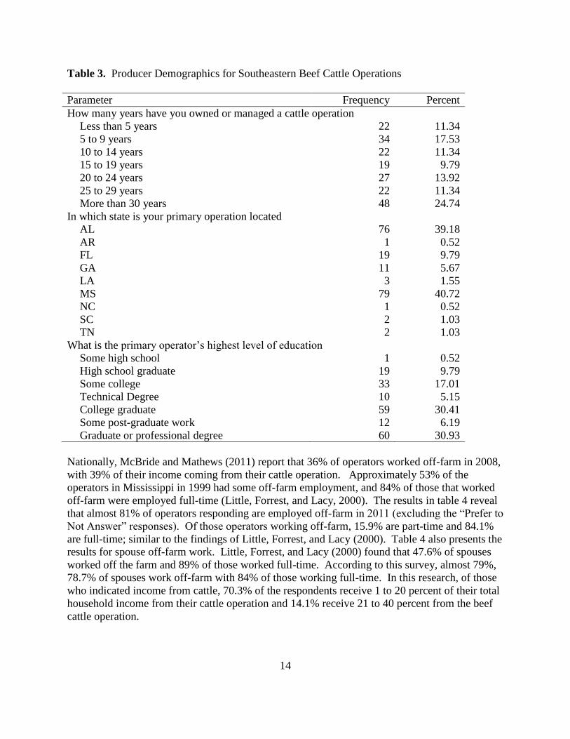
Table 3. Producer Demographics for Southeastern Beef Cattle Operations

Parameter Frequency Percent

How many years have you owned or managed a cattle operation

Less than 5 years 22 11.34

5 to 9 years 34 17.53

10 to 14 years 22 11.34

15 to 19 years 19 9.79

20 to 24 years 27 13.92

25 to 29 years 22 11.34

More than 30 years 48 24.74

In which state is your primary operation located

AL 76 39.18

AR 1 0.52

FL 19 9.79

GA 11 5.67

LA 3 1.55

MS 79 40.72

NC 1 0.52

SC 2 1.03

TN 2 1.03

What is the primary operator’s highest level of education

Some high school 1 0.52

High school graduate 19 9.79

Some college 33 17.01

Technical Degree 10 5.15

College graduate 59 30.41

Some post-graduate work 12 6.19

Graduate or professional degree 60 30.93

Nationally, McBride and Mathews (2011) report that 36% of operators worked off-farm in 2008,

with 39% of their income coming from their cattle operation. Approximately 53% of the

operators in Mississippi in 1999 had some off-farm employment, and 84% of those that worked

off-farm were employed full-time (Little, Forrest, and Lacy, 2000). The results in table 4 reveal

that almost 81% of operators responding are employed off-farm in 2011 (excluding the “Prefer to

Not Answer” responses). Of those operators working off-farm, 15.9% are part-time and 84.1%

are full-time; similar to the findings of Little, Forrest, and Lacy (2000). Table 4 also presents the

results for spouse off-farm work. Little, Forrest, and Lacy (2000) found that 47.6% of spouses

worked off the farm and 89% of those worked full-time. According to this survey, almost 79%,

78.7% of spouses work off-farm with 84% of those working full-time. In this research, of those

who indicated income from cattle, 70.3% of the respondents receive 1 to 20 percent of their total

household income from their cattle operation and 14.1% receive 21 to 40 percent from the beef

cattle operation.

15

Table 4. Household Income Structure for Southeastern Beef Cattle Operations

Parameter Frequency Percent

Which of the following best describes your 2010 total household net income?

Less than $30,0000 8 4.12

$30,000 to $59,999 38 19.59

$60,000 to $89,999 46 23.71

$90,000 to $119,999 44 22.68

More than $120,000 38 19.59

Prefer to not answer 20 10.31

Approximately what percentage of your 2010 household net income came from your

beef cattle operation?

0 percent 18 9.28

1 to 20 percent 129 66.49

21 to 40 percent 26 13.41

41 to 60 percent 6 3.09

61 to 80 percent 3 1.55

81 to 99 percent 1 0.52

100 percent 1 0.52

Prefer to not answer 10 5.15

What is the extent of off-farm work for the primary operator?

No off-farm work 37 19.07

Part-time off-farm work 25 12.89

Full-time off-farm work 132 68.04

What is the extent of off-farm work for the spouse of the primary operator (if

applicable)?

No off-farm work 31 15.98

Part-time off-farm work 19 9.79

Full-time off-farm work 99 51.03

Not Applicable 45 23.20

Table 5 details the summary statistics for weaning weight and rate weaning age, and breeding

success. The results of this study found the mean weaning weight of male calves for the herds of

122 respondents to be almost 553 pounds. The NAHMS (USDA, APHIS, 2008) study reports an

average weaning weight for male calves in the East region (the region most identical to the one

used in this survey) as 531 pounds. The NAHMS national average weaning weight for male

calves across all beef cattle operations was reported as 559 pounds; by operation size, herds of 1

to 49 head produced male calves of 532 pounds at weaning and herds with 100-199 head

produced male calves of 572 pounds at weaning. The mean weaning age for calves in the

NAHMS study was approximately 200 days, or 6.67 months, for the East region and 207 days

across all regions in the USDA survey (USDA, APHIS, 2008). For 131 herds in the present

study the mean weaning age was 6.77 months, or 203 days based on a 30-day month.

This study calculated the birth-to-weaning rate as a ratio of the weaning rate (weaned calves

compared to exposed breeding females) to pregnancy rate (cows that conceived per exposed

16

breeding females). To clarify: the birth-to-weaning rate is defined as the number of calves that

survived from birth to weaning based on the number of cows that conceived. For example, if an

operator has 100 cows that are exposed for breeding and 95 of them become pregnant, the

pregnancy rate is 95%. If, of those 95 cows, 90 give birth to a live calf, the calving rate (calves

born per cows exposed) is 90%; and if 88 of those 90 survive to weaning, the weaning rate

(calves weaned per cows exposed) is 88%. The birth-to-weaning rate captures, instead, the

number of calves that are weaned based on the number of cows that actually become pregnant.

This allows the researcher to account only for management of the pregnant cow and subsequent

live-born calf and does not capture management of exposed females that do not conceive. This

research is generally concerned with the optimal management of the calf after conception (but

not to the exclusion of reproductive performance) to achieve the product of the operation: pounds

of beef weaned. Considering the same 95 pregnant cows and 88 weaned calves from the

example above, the birth-to-weaning rate would be 88 divided by 95, or 92.6%.

Table 5. Summary Statistics for Cow-Calf Weights and Rates and Weaning Age

Parameter Mean

Standard

Deviation Minimum Maximum N

Cow herd pregnancy rate (percent)1

Average 89.0 6.3 65.0 100.0 110

Calf death loss at birth (percent)2

Average 2.8 9.5 0.0 99.0 109

Cow herd weaning rate (percent)3

Average 89.7 7.7 60.0 100.0 101

Birth-to-weaning rate (percent)4

98.3 3.4 84.0 100.0 101

Calf weaning age (months)

6.8 1.0 4.0 9.0 131

Weaning weight for male calves (in pounds)

Average 552.7 87.4 350.0 800.0 122

Brood cow weight (in pounds)

Average 817.7 316.0 325.0 1800.0 123

1Total breeding cows pregnant as a percentage of exposed cows.

2Number of calves that die within 24 hours of birth as a percentage of total calves born.

3Number of calves weaned as a percentage of exposed breeding cows.

4Number of calves weaned as a percentage of calves conceived (average weaning rate/average pregnancy rate).

The mean birth-to-weaning rate in this study is 98.3%. The birth-to-weaning ratio used in this

survey is a unique value and therefore, makes comparison of this result to any regional or

national average responses pointless. It implies that for every 100 cows that conceive,

approximately 98 of them will give birth to calves that make it to weaning. There is a conflict in

this research with the average death loss figure of 2.8%, suggesting that the birth-to-weaning

ratio may be a bit inflated due to survey response error.

17

The average death loss from the present research is 2.8%. The national average was 3.6% and

the Southeast region (the region in this NAHMS study that is most identical to the Southeast

region in the present research) death loss was reported at 3.1% (USDA, APHIS, 2010a). Part

five of the NAHMS (2010b) study reports the national average death loss for the first half of

2008 as 3.2% and the Southeast regional average as 2.5%. The 2.8% in the present research is

within .03% of the two southeast regional averages reported in parts four and five of the

NAHMS study (USDA, APHIS, 2010a; 2010b).

Part three of the NAHMS (USDA, APHIS, 2009) reports a national average calving percentage

of 92.4%, 92.6%, and 91.5% for 1992-1993, 1997, and 2007-2008, respectively. The calving

percentage contained in the NAHMS study does not include pregnant heifers and cows that were

sold or moved off of the operation, causing it to possibly be slightly higher than a true pregnancy

rate. In 2007, 3.1% of pregnant beef cows left the average operation (USDA, APHIS, 2009a).

This suggests an approximate average pregnancy rate in 2007 of 88.4% nationally (91.5%

calving rate less 3.1% pregnant cows moved off the operation). However, the survey results in

table 5 show an 89% pregnancy rate, suggesting similar results to the 2007 national averages.

Figure 2 illustrates the percent of cattle operations in each region, as mapped in figure 1, by the

number of head per farm (USDA, NASS, 2007).

Figure 2. Percent of Cattle Operations by Herd Size, 2007

The results of the survey questions that asked for herd size and makeup are presented in table 6.

The primary results for discussion are the size categories of the commercial cow herds. The

Agricultural Census of 2007 (USDA, NASS, 2007), reports that the number of operations in the

18

Southeast with 1 to 49 head comprised 83.9% of all beef cattle operations in the region. Those

operations in all of the U.S. with 1 to 49 head comprised 79.4% of all beef cattle operations. The

Northern Plains (map area 6 in figure 1) had the lowest percentage of total beef cattle farms with

only 54.4%. Only 5.8% of operations in the Southeast had more than 100 head. The results in

Table 5.4 show that about 52.7% of all cattle operations in the Southeast had 1 to 49 head and

24.8% of all respondents with commercial cow herds had 50 to 99 head (excludes “No response”

and “0” responses). Operations with more than 100 head in the herd comprise 22.4% of the

operations responding to the survey in this research. The difference between the results of this

survey and the results reported in the 2007 Agricultural Census (USDA, NASS, 2007) could be

due to the time of year in which responses were collected or the type of survey delivery used.

Survey respondents also reported on the number of head, if applicable, in a seedstock herd, the

number of stocker cattle owned, the number of head in a feedlot for finishing or being custom

backgrounded, and the number of head that were dedicated for freezer beef or sold direct-to-

customer. Seedstock operations of 1 to 49 head made up 72.9%, 50 to 99 head was 16.1%, and

more than 100 head was 11% of all operators with a seedstock herd.

Only 36.6% of respondents reported owning stocker cattle. Of those, nearly 61% had 1 to 49

head of stocker cattle and the other 39% had more than 100 head. No operators responded

positively to owning a stocker herd of 50 to 99 head. Approximately 77% of respondents that

owned or managed custom backgrounded herds reported having 1 to 49 head and the remaining

23% had herds from 50 to 1,999 head. Twenty-seven respondents reported ownership of feedlot

cattle; 70% owned 1 to 49 head and 30% reported 50 to 499 head. Fifty-eight operators reported

freezer beef or direct-to-customer sales; fifty-one, nearly 88%, utilized 1 to 9 head for these

purposes.

Table 6. Summary Statistics of Cow-Calf Operations—Herd Type and Size

Parameter Frequency Percent

Total number of commercial cows (breeding age females only) N=194

No response 6 3.09

0 23 11.86

1 to 9 14 7.22

10 to 29 34 17.53

30 to 49 39 20.10

50 to 74 34 17.53

75 to 99 7 3.61

100 to 149 18 9.28

150 to 199 6 3.09

200 to 299 5 2.58

300 to 499 4 2.06

500 to 999 3 1.55

1000 or more 1 0.52

19

Table 6. (Continued)

Parameter Frequency Percent

Total number of seedstock cows (breeding age females only) N=194

No response 6 3.09

0 70 36.08

1 to 9 31 15.98

10 to 29 31 15.98

30 to 49 24 12.37

50 to 74 9 4.64

75 to 99 10 5.15

100 to 149 5 2.58

150 to 199 2 1.03

200 to 299 1 0.52

300 to 499 4 2.06

500 to 999 0 0.00

1000 or more 1 0.52

Total number of stocker cattle owned N=194

No response 6 3.09

0 117 60.31

1 to 49 43 22.16

50 to 99 0 6.19

100 to 199 6 3.09

200 to 499 6 3.09

500 to 999 3 1.55

1,000 to 4,999 0 0.00

5,000 to 9,999 1 0.52

10,000 or more 0 0.00

Total number of custom backgrounded head managed N=194

No response 6 3.09

0 135 69.59

1 to 9 15 7.73

10 to 29 19 9.79

30 to 49 7 3.61

50 to 74 2 1.03

75 to 99 1 0.52

100 to 149 3 1.55

150 to 199 2 1.03

200 to 299 2 1.03

500 to 999 1 0.52

1,000 or1,999 1 0.52

2,000 or more 0 0.00

20

Table 6. (Continued)

Parameter Frequency Percent

Total number of head placed in a feedlot for finishing N=194

No response 6 3.09

0 161 82.99

1 to 49 19 9.79

50 to 99 6 3.09

100 to 199 1 0.52

200 to 499 1 0.52

500 to 999 0 0.00

1,000 to 1,9999 0 0.00

2,000 to 4,9999 0 0.00

5,000 to 9,999 0 0.00

10,000 to 19,999 0 0.00

20,000 or more 0 0.00

Total number of head for freezer beef or direct-to-consumer sales N=194

No response 6 3.09

0 130 67.01

1 to 9 51 26.29

10 to 29 5 2.58

30 to 49 2 1.03

50 to 74 0 0.00

75 to 99 0 0.00

100 to 149 0 0.00

150 to 199 0 0.00

200 to 299 0 0.00

300 to 499 0 0.00

500 or more 0 0.00

Results of Regression Models

Table 7 gives the results of the regression performed using equation [1]. The overall F-statistic

for the model is 2.54 (Pr>F 0.0015) and the R2 value is 0.321. The results from this regression

demonstrate the importance of weaning age on the weight of a weaned calf. Weaning age has a

positive effect on the weaning weight of a calf, following the a priori assumptions based on Pell

and Thayne (1978). Weaning age is significant at = 0.01. The significance of WEANAGE

also points to increased weight gain as the calf is weaned at a later age. This increase in the

growth relationship between weaning age and weaning weight was found to be significant in the

research of Pell and Thayne (1978). It is best described by a curved line with a non-constant

increase up to 300 days of age.

21

Table 7. Weaning Weight Results from Equation 1

Variable

Significance

Level

Parameter

Estimate

Standard

Error t Value Pr > |t|

Intercept 403.150 74.154 5.440 <.0001

EXP29 14.441 17.680 0.820 0.416

EXP30 0.203 20.591 0.010 0.992

BEEFINC21 29.561 20.154 1.470 0.146

CC49 ** -77.670 30.263 -2.570 0.012

CC199 ** -77.831 31.483 -2.470 0.015

CC200 *** -75.054 39.643 -1.890 0.061

SS49 ** 42.686 17.611 2.420 0.017

SS199 ** 61.627 28.881 2.130 0.035

SS200 *** 90.197 45.980 1.960 0.053

FIN21 19.996 21.776 0.920 0.361

RYE -17.436 17.222 -1.010 0.314

WIN 9.243 21.208 0.440 0.664

SPR -12.595 23.753 -0.530 0.597

SUM -16.593 21.980 -0.750 0.452

FALL -3.966 20.703 -0.190 0.849

CALFMON3 2.474 20.532 0.120 0.904

CALFSEA2 -31.209 30.467 -1.020 0.308

SUPPCALF 16.911 15.474 1.090 0.277

WEANAGE * 28.161 7.810 3.610 0.001 * Significant at = 0.01. Fstat = 2.54

** Significant at = 0.05. R2 = 0.321

***Significant at = 0.10. N = 122

The variables for commercial herd size and seedstock herd size are each significant at = 0.05

for CC49, CC199, SS49, and SS199. The variables, CC200 and SS200 are significant at =

0.10. The parameter estimates for these variables should be interpreted as a comparison of

commercial cow herd influence versus seedstock herd influence. For example, the parameter

estimate for SS200 implies 90.1968 additional pounds to be gained on the weaning intercept

compared to the similar commercial cow category. Generally, dummy variables are interpreted

on a base dummy category; in this case, CC49, CC199, and CC200 are compared to a seedstock

only operation of the same size. Also, SS49, SS199, and SS200 are compared to a commercial

only operation. This comparison shows the weaning weight premium that may result from

seedstock cattle being heavier, purebred breeds. Commercial cow producers with 1 to 49, 50 to

199, and more than 200 head will produce a calf that weans 77.7, 77.8, and 75.1 pounds,

respectively, lighter than seedstock herds of the same size. Seedstock herds of 1 to 49, 50 to 199,

and more than 200 head will have an average weaning weight of about 43, 62 and 90 pounds,

respectively, greater than like-sized commercial cow herds.

An F-test was performed on the commercial cow and seedstock categories. The null hypothesis

for the first test was: 0 : 49 199 200H CC CC CC . The resulting F-statistic for the test was

22

0.00 (Pr>F 0.996), so the null hypothesis was rejected. For the seedstock variables, the null

hypothesis was: 0 : 49 199 200H SS SS SS and the F-statistic was 0.63 (Pr>F 0.536); the null

hypothesis was rejected. White’s test for heteroscedasticity in the regression of equation [1]

yielded a 2

stat result of 1.60 (Pr>ChiSq 0.45); heteroscedasticity was not detected in the results.

Table 8. Weaning Weight Variability Results from Equation 4.2

Variable

Significance

Level

Parameter

Estimate

Standard

Error t Value Pr > |t|

Intercept -12.169 29.407 -0.410 0.680

EXP29 ** 16.585 6.751 2.460 0.016

EXP30 3.804 7.639 0.500 0.620

BEEFINC21 7.249 7.889 0.920 0.361

CC49 1.032 11.593 0.090 0.929

CC199 -8.911 11.941 -0.750 0.458

CC200 -1.871 15.851 -0.120 0.906

SS49 4.146 6.761 0.610 0.541

SS199 12.064 11.368 1.060 0.292

SS200 11.891 16.647 0.710 0.477

FIN21 5.440 8.412 0.650 0.520

RYE -0.924 6.771 -0.140 0.892

WIN -1.876 8.201 -0.230 0.820

SPR 13.502 9.025 1.500 0.138

SUM 11.094 8.368 1.330 0.188

FALL 13.328 8.145 1.640 0.105

CALFMON3 0.024 7.670 0.000 0.998

CALFSEA2 -17.626 11.392 -1.550 0.125

SUPPCALF -3.365 5.880 -0.570 0.569

WEANAGE *** 5.349 3.045 1.760 0.082 * Significant at = 0.01. Fstat = 1.22

** Significant at = 0.05. R2 = 0.207

***Significant at = 0.10. N = 109

The variance inflation factors (VIF) were calculated and none exceeded 5.0 for any of the

variables, so no high degree of multicollinearity was detected. Operator experience, calving

season timing and length, number of calving seasons, supplemental feeding of creep-fed calves,

the use of cool annual rye, income and financing level show no significant on weaning weight as

regressed in this equation.

Table 8 contains the results of the regression of the standard deviation of the weaning weight,

equation [2]. The properties of the triangular distribution were used to determine the variance of

weaning weight in an individual herd, then the standard deviation of the low, high, average group

of weaning weight responses. This regression is important in that it examines the factors that

directly affect the variability of the key product, pounds of beef weaned, in a cow-calf enterprise.

The overall F-statistic for the model is 1.22 (Pr>F 0.258) and the R2 value is 0.207. The F-

23

statistic alone indicates that this model, as constructed, may not adequately explain the factors

that affect weaning weight variability.

The two variables of significance were the ones representing 15 to 29 years of experience

(EXP29) and WEANAGE. EXP29 has a significant positive effect, at = 0.05, on the

variability of weaning weight. This level of experience increases the variability in weaning

weight by 16.6 pounds compared to those operators with 1 to 14 years of experience. The cause

for such an increase compared to those lesser-experienced operators is difficult to explain and

seems to contradict the conventional wisdom that more experienced operators manage their herds

closer.

The weaning age (WEANAGE) also has a significant, at = 0.10, effect, increasing variability

by 5.35 pounds for every additional month that weaning is postponed. As a calf ages, the weight

of any given group of calves becomes more spread out. For example, humans may be born

weighing 6 to 11 pounds but by 30 years of age, the weight may be spread from 75 pounds to

more than 500 pounds; significant variability. The birth weight of a calf will fall into a relatively

tight range of weights, but by six to seven months of age many factors have been able to

influence its growth and cause the range of weaning weights to spread. No other variables in this

equation have significant effect on the variability of weaning weight within an individual herd.

The 2

stat of 0.48 in White’s test indicated no notable presence of heteroscedasticity. The VIF for

each of the variables did not exceed 5.0 so indicating that no high degree of multicollinearity

exists in the results of equation [2].

Table 9 reveals the significance of 49 or fewer head of commercial or seedstock cattle in relation

to the birth-to-weaning rate (B2W) of the herd. The categorical interpretation here is similar to

that of table 7. The variables CC49 and SS49 both show significance at the = 0.10 level. No

other variables in these results show significance at = 0.10 or smaller. Commercial cow-calf

producers with 1 to 49 head have a 22% lower birth-to-weaning rate than those producers who

own solely seedstock cattle. Conversely, seedstock producers with 1 to 49 head can expect to

have a birth-to-weaning rate increase of 13.5% over those operators with only commercial cow-

calf herds. Small commercial cow producers have a lower birth-to-weaning rate than seedstock

producers and seedstock producers have a higher B2W than commercial cow producers. The

relative success of small seedstock producers may be due to the genetic makeup of their herd;

often purebred cattle.

The F-statistic for the model is 1.24 (Pr>F 0.255) and the R2 value is 0.182. These two values

together indicate that the explanatory variables, as specified, may not significantly explain the

variation in the birth-to-weaning rate.

Pregnancy rate is defined as the number of cows that conceive per number of exposed breeding

females in the herd. Ramsey, et al. (2005) show that positive changes in calving percentage

(resulting from positive changes in pregnancy rates) increase the profitability of an operation.

The regression results in table 10 have a model F-statistic of 1.08 (Pr>F 0.384) and an R2 value

of 0.157. These results indicate that the regression equation used to obtain the results may not be

correctly specified.

24

Table 9. Birth-to-Weaning Rate Results from Equation 4.3

Variable

Significance

Level

Parameter

Estimate

Standard

Error t Value Pr > |t|

Intercept 1.073 0.218 4.910 <.0001

EXP29 0.055 0.082 0.670 0.504

EXP30 -0.003 0.088 -0.030 0.973

BEEFINC21 -0.071 0.086 -0.830 0.407

CC49 *** -0.220 0.122 -1.800 0.075

CC199 -0.034 0.126 -0.270 0.790

CC200 -0.113 0.161 -0.700 0.483

SS49 *** 0.135 0.077 1.760 0.082

SS199 -0.002 0.129 -0.010 0.989

SS200 0.135 0.190 0.710 0.479

FIN21 -0.031 0.097 -0.320 0.751

WIN -0.117 0.092 -1.280 0.205

SPR 0.071 0.111 0.640 0.525

SUM 0.061 0.105 0.580 0.561

FALL 0.029 0.103 0.280 0.781

CALFMON3 0.055 0.091 0.600 0.547

CALFSEA2 -0.103 0.133 -0.780 0.439 * Significant at = 0.01. Fstat = 1.24

** Significant at = 0.05. R2 = 0.182

***Significant at = 0.10. N = 106

The plot of residuals versus predicted values for this model indicated potential heteroscedasticity

in the error terms in the pregnancy rate model. Based on the graphical observation of the

residuals, White’s test was used to detect heteroscedasticity in the results. The of 86.69

and Pr>F = 0.6368 indicates that there is no heteroscedasticity. White’s general test for

heteroscedasticity was used in each of the sets of results. The variance inflation factors (VIF)

were calculated and the presence of a high degree of multicollinearity between any of the

variables in the equation was not detected.

The results reveal that the response variable for operators that derive 21% or more of their

income from their cattle operation (BEEFINC21) is significantly different from zero at = 0.05.

If an operator derives 21% or more of total income from the cattle operation, pregnancy rate

increases 3.3% over the mean of 88.9%. The significance and sign of the BEEFINC variable

seems to indicate that the higher investment in the farm, the greater attention the operator gives

to the success of the herd. Only 37 operations, of the 166 respondents reporting cattle income,

derive 21% or more of their income from the cattle operation.

25

Table 10. Pregnancy Rate Results from Equation 4.4

Variable

Significance

Level

Parameter

Estimate

Standard

Error t Value Pr > |t|

Intercept 0.889 0.042 21.240 <.0001

EXP29 0.009 0.015 0.590 0.560

EXP30 0.004 0.017 0.230 0.817

BEEFINC21 ** 0.033 0.017 1.870 0.064

CC49 -0.016 0.023 -0.680 0.500

CC199 -0.011 0.024 -0.450 0.652

CC200 -0.012 0.031 -0.390 0.696

SS49 0.008 0.014 0.580 0.560

SS199 -0.006 0.025 -0.250 0.802

SS200 0.030 0.037 0.810 0.420

FIN21 -0.024 0.019 -1.260 0.213

WIN -0.014 0.018 -0.810 0.421

SPR -0.010 0.019 -0.560 0.577

SUM 0.024 0.019 1.250 0.215

FALL 0.008 0.018 0.440 0.664

CALFMON3 0.026 0.018 1.480 0.142

CALFSEA2 -0.008 0.021 -0.370 0.712 * Significant at = 0.01. Fstat = 1.08

** Significant at = 0.05. R2 = 0.157

***Significant at = 0.10. N = 110

The model for weaning rate variability, equation [5], also shows few significant variables. These

are reported in table 11. This model has an F-statistic of 0.75 (Pr>F 0.736) and an R2 of 0.146.

These two values, considered together, indicate that the explanatory variables, as specified, may

not significantly explain the variation in the weaning rate variability.

The one variable of significance in the regression results of equation 5 is FIN21; which

represents those operators that finance 21% or more of their cattle and feed. FIN21 is signed

negative and is significant at = 0.10. It is a dummy variable, and should be interpreted as

compared to the base category of zero to 20% financed. In these results, if 21% or more of the

cattle and feed are financed by outside sources, the mean variability of weaning rate is decreased

by 1.5% compared to an operator that is financing less than 21% of their feed and cattle costs.

The significance and sign of FIN21 seems to indicate that an operator that is invested in their

operation with more than 21% outside financing is more attentive to the outcome of the

production process than those that finance less than 20% of their cattle and feed.

White’s general test was used to detect the presence of heteroscedasticity and the variance

inflation factors were generated to detect a high degree of multicollinearity; neither of these

issues existed in the results.

26

Table 11. Weaning Rate Variability Results from Equation 4.5

Variable

Significance

Level

Parameter

Estimate

Standard

Error t Value Pr > |t|

Intercept 3.449 1.798 1.920 0.059

EXP29 -0.160 0.649 -0.250 0.806

EXP30 -0.007 0.697 -0.010 0.992

BEEFINC21 0.380 0.738 0.510 0.609

CC49 -0.881 1.049 -0.840 0.404

CC199 -0.862 1.091 -0.790 0.432

CC200 -1.302 1.299 -1.000 0.320

SS49 -0.143 0.605 -0.240 0.814

SS199 -0.489 1.188 -0.410 0.682

SS200 -1.105 1.441 -0.770 0.446

FIN21 *** 1.507 0.760 1.980 0.051

WIN 0.775 0.758 1.020 0.311

SPR 0.174 0.893 0.200 0.846

SUM -1.279 0.891 -1.440 0.156

FALL -1.039 0.886 -1.170 0.245

CALFMON3 0.401 0.721 0.560 0.580

CALFSEA2 0.978 1.057 0.920 0.358 * Significant at = 0.01. Fstat =0.75

** Significant at = 0.05. R2 = 0.146

***Significant at = 0.10. N = 87

Conclusions and Implications

The first objective of this study was to characterize current cow-calf operations in the

southeastern United States. This was compared with results of past research related to beef cattle

operations in this region. This was also compared with the results of current national statistics.

Frequency counts and percentages as well as the common summary statistics of mean and

standard deviation provided the details of the results for these two objectives. The characteristics

of southeastern beef cattle operations are different in the results of this research in average size

and demographic when compared to results from past research. A larger percentage of operators

and their spouses are now working off of the farm for income. The national average of 36%

from McBride and Mathews (2011)—taken from 2008 data—differs from the results of this

research in which average off-farm employment was near 81%. The prevalence of small farms

with less than 49 head of beef cattle remains similar to prior years. Part three of the NAHMS

(USDA, APHIS, 2009) study reported 81% of operations had 49 or fewer head in 1992 and

79.1% in 2007. The results of this research reveal that over 53% of commercial operators have

fewer than 49 head and 72.9% of seedstock operators have fewer than 49 head.

The second objective for this research was to examine factors affecting production on beef calf

operations in the Southeast. The third objective was to examine the within-herd production risks

associated with variability in weaning weight—the product of the operation—and weaning rate.

27

Those models were constructed using dependent and explanatory variables found in previous

research literature. The weaning age of calves has significant positive effect on the weaning

weight of calves and on the variability of pounds of beef weaned. An additional month in

weaning age leads to a gain of 28 pounds in the weight of the calf but can also increase the

standard deviation of weaning weight by 5.3 pounds. The signs of the explanatory variables in

each of the models follow prior research and the a priori assumptions with few exceptions.

The results of the research merit further examination to define the differences in variability

between seedstock operators and commercial cow-calf operators, cow-calf only versus cow-

calf/stocker operations, and perhaps a comparison of operations by state. Additionally, soliciting

answers to derive the triangular distribution for pregnancy rates, weaning weights and rates, and

death loss rates within individual herds, would provide a foundation for examination of the

causes of variability in those factors. This would allow individual operators to perhaps improve

management practices, herd makeup, or other production factors to gain more pounds of beef

weaned and thus, a greater profit.

The results of this research provide a beef cattle operator in the Southeast an analysis of factors

that affect production through pregnancy rate, weaning weight, and the birth-to-weaning rate.

The lack of significance in some of the models provides the opportunity for extended data

collection to perhaps improve results of the models. This research has also provided a

foundational body of work on which to build future cattle industry research for the Southeast.

The factors that affect cattle production have been extensively explored in this work and can be

built on as further research is completed. The producer demographics and operation data

collected provides extension personnel have current data to describe the southeastern beef cattle

operation.

Past research has included operator age and experience. Inclusion of a variable to capture age of

the operator could add to the demographic information but could also possibly aid in partially

explaining some of the production practices and issues. Age is a common question that was not

used in this research. Questions for direct calving rate, pregnant heifers and cows taken off of

the operation, and artificial insemination success rates could help to explain reproductive and

weaning efficiency. Those questions were not used in this research.

Empirical model development demands the use of foundational economic research; that past

research reveals a large number of factors that influence the production criteria that were

examined in this research. It is difficult, particularly through an online survey instrument, to

capture all of the primary variables that affect weaning rate, for example, without encountering

models that require a large number of explanatory variables. The controlled discipline of animal

science research is well-equipped to capture the biological and physiological data that is needed.

28

References

Ball, Donald M., Carl S. Hoveland, and Garry D. Lacefield. 1996. Southern Forages: Modern

Concepts for Forage Crop Management. Norcross, GA: Potash and Phosphate Institute.

Buskirk, D. D., D. B. Faulkner, and F. A. Ireland. 1995. Increased Postweaning Gain of Beef

Heifers Enhances Fertility and Milk Production. Journal of Animal Science 73: 937-946.

Cundiff, L. V., R. L. Willham, and Charles A. Pratt. 1966. Effects of Certain Factors and Their

Two-Way Interactions on Weaning Weight in Beef Cattle. Journal of Animal Science 25: 972-

982.

Dargatz, David A., Grant A. Dewell, and Robert G. Mortimer. 2004. Calving and Calving

Management of Beef Cows and Heifers on Cow-Calf Operations in the United States.

Theriogenology 61: 997-1007.

Dhuyvetter, Kevin, and Michael Langemeier. January 2010. Differences Between High,

Medium, and Low Profit Cow-Calf Producers: An Analysis of 2004-2008 Kansas Farm

Management Association Cow-Calf Enterprise. Agmanager.info.

http://www.agmanager.info/livestock/budgets/production/beef/Cow-

calf_EnterpriseAnalysis(Jun2009)--Revised(Jan2010).pdf (accessed December 2010).

Doren, P. E., C. R. Long, and T. C. Cartwright. 1986. Factors Affecting the Relationship

Between Calving Interval of Cows and Weaning Weights of Calves. Journal of Animal Science

62: 1194-1202.

Gaertner, S. J., Jr., F. M. Rouquette, D. R. Long, and J. W. Turner. 1992. Influence of Calving

Season and Stocking Rate on Birth Weight and Weaning Weight of Simmental-Sired Calves

From Brahman-Hereford F1 Dams. Journal of Animal Science 70: 2296-2303.

Informa Economics. April 18, 2011. "US Beef Producers Weigh Options." Policy Report.

Little, Randall D., Charlie S. Forrest, and R. Curt Lacy. 2000. “Cattle Producer Attitudes

Towards Alternative Production and Marketing Practices”. Departmental Research Report,

Agricultural Economics, Mississippi State University.

McBride, William D., and Kenneth Mathews, Jr. 2011. The Diverse Structure and Organization

of U.S. Beef Cow-Calf Farms. Washington DC: U.S. Department of Agriculture, March.

Pell, E. W., and W. V. Thayne. 1978. Factors Influencing Weaning Weight and Grade of West

Virginia Beef Calves." Journal of Animal Science 46: 596-603.

Popp, Michael P., and Lucas D. Parsch. 1998. “Production Practices of Arkansas Beef Cattle

Producers”. University of Arkansas Agr. Exp. Sta. Res. Bull. No. 956, January.

29

Ramsey, Ruslyn, Damona Doye, Clement Ward, James McGrann, Larry Falconer, and Stanley

Bevers. 2005. Factors Affecting Beef Cow-Herd Costs, Production, and Profits. Journal of

Agricultural and Applied Economics 37(1): 91-99.

Sellers, H. I., R. L. Willham, and R. C. deBaca. 1970. Effect of Certain Factors on Weaning

Weight of Beef Calves. Journal of Animal Science. 31: 5-12.

Troxel, T. R.; Lusby, K. S.; Gadberry, M. S.; Barham, B. L.; Poling, R.; Riley, T.; Eddington, S.;

Justice, T. 2007. The Arkansas Beef Industry--A Self-Assesment. The Professional Animal

Scientist 23: 104-115.

U.S. Departement of Agriculture, Animal and Plant Health Inspection Service, (USDA, APHIS).

June 1997. Animal Health.

http://www.aphis.usda.gov/animal_health/nahms/beefcowcalf/index.shtml#beef97 (accessed

March 1, 2011).

U.S. Department of Agriculture. 2008. Beef 2007-08, Part I: Reference of Beef Cow-calf

Management Practices in the United States, 2007-08. Fort Collins, CO: USDA-APHIS-VS,

CEAH. N512-1008, October.

—. 2009. Beef 2007-08, Part III: Changes in the U.S. Beef Cow-Calf Industry, 1993-2008. Fort

Collins, CO: USDA-APHIS-VS, CEAH. 518-0509, May.

—. 2010a. Beef 2007-08, Part IV: Reference of Beef Cow-calf Management Practices in the

United States, 2007-08. Fort Collins, CO: USDA-APHIS-VS, CEAH. 523-0210, February.

—. 2010b. Beef 2007-08, Part V: Reference of Beef Cow-calf Management Practices in the

United States, 2007-08. Fort Collins, CO: USDA-APHIS-VS, CEAH. 532-0410, April.

U.S. Department of Agriculture, National Agricultural Statistics Service, (USDA, NASS).

February 3, 2007. 2007 Census Publications. USDA-NASS 2007 Census of Agriculture.

http://www.agcensus.usda.gov/Publications/2007/Full_Report/Volume_1,_Chapter_2_US_State

_Level/st99_2_011_011.pdf (accessed October 2010).

—. 2011. Quick Stats. QuickStats 2.0 Beta.

http://quickstats.nass.usda.gov/?source_desc=CENSUS (accessed April 2011).

White, H. 1980. A Heteroscedasticity Consistent Covariance Matrix Estimator and a Direct

Test of Heteroscedasticity. Econometrica 48: 817-818.

Wittum, T. E., C. R. Curtis, M. D. Salman, M. E. King, K. G. Odde, and R. G. Mortimer. 1990.

Management Practices and Their Association with Reproductive Health and Performance in

Colorado Beef Herds. Journal of Animal Science 68: 2642-2649.