Embed Size (px)
Citation preview
Tracing biogeochemical processes using sulfur stable isotopes:
two novel applications
by
Mélanie Lyne Cousineau
A thesis submitted
to the Faculty of Graduate and Postdoctoral Studies
in partial fulfilment of the requirements for the degree of
Ph.D. in Earth Sciences,
Specialisation in Chemical and Environmental Toxicology
University of Ottawa
Ottawa, Ontario
© Mélanie Lyne Cousineau, Ottawa, Canada, 2013

We have not succeeded in answering all our problems. The answers we
have found only serve to raise a whole set of new questions. In some ways,
we feel we are as confused as ever, but we believe we are confused
on a higher level, and about more important things.
Attributed to Earl C. Kelly, 1951.
— iii —
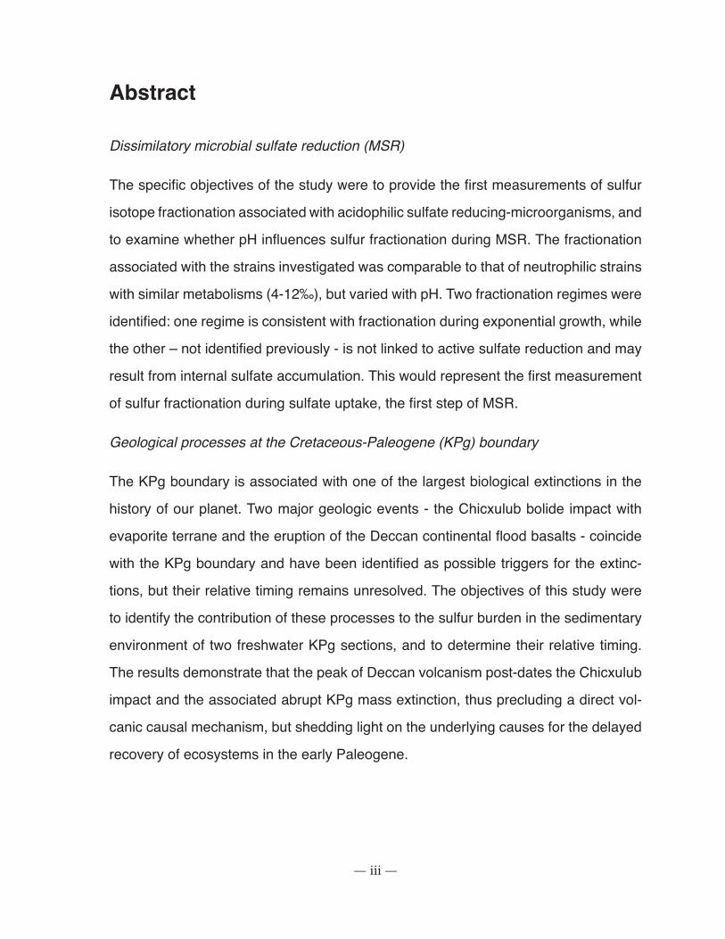
Abstract
Dissimilatory microbial sulfate reduction (MSR)
The specific objectives of the study were to provide the first measurements of sulfur
isotope fractionation associated with acidophilic sulfate reducing-microorganisms, and
to examine whether pH influences sulfur fractionation during MSR. The fractionation
associated with the strains investigated was comparable to that of neutrophilic strains
with similar metabolisms (4-12‰), but varied with pH. Two fractionation regimes were
identified: one regime is consistent with fractionation during exponential growth, while
the other – not identified previously - is not linked to active sulfate reduction and may
result from internal sulfate accumulation. This would represent the first measurement
of sulfur fractionation during sulfate uptake, the first step of MSR.
Geological processes at the Cretaceous-Paleogene (KPg) boundary
The KPg boundary is associated with one of the largest biological extinctions in the
history of our planet. Two major geologic events - the Chicxulub bolide impact with
evaporite terrane and the eruption of the Deccan continental flood basalts - coincide
with the KPg boundary and have been identified as possible triggers for the extinc-
tions, but their relative timing remains unresolved. The objectives of this study were
to identify the contribution of these processes to the sulfur burden in the sedimentary
environment of two freshwater KPg sections, and to determine their relative timing.
The results demonstrate that the peak of Deccan volcanism post-dates the Chicxulub
impact and the associated abrupt KPg mass extinction, thus precluding a direct vol-
canic causal mechanism, but shedding light on the underlying causes for the delayed
recovery of ecosystems in the early Paleogene.
— iv —
Résumé
Réduction microbienne non-assimilatoire des sulfates (RMS)
Les objectifs spécifiques de cette étude étaient d’effectuer les premières mesures
du fractionnement isotopique du soufre associé à la réduction des sulfates par des
micro-organismes acidophiles et d’examiner le rôle du pH dans le fractionnement
durant la RMS. Le fractionnement associé aux souches étudiées est comparable à
celui de souches neutrophiles à métabolisme semblable (4-12‰), mais varie en fonc-
tion du pH. Deux régimes de fractionnement ont été identifiés: l’un est en accord avec
le fractionnement durant la phase exponentielle de croissance, alors que l’autre - qui
n’avait pas été identifié précédemment - n’est pas associé à la réduction active de
sulfates et pourrait résulter de leur accumulation à l’intérieur de la cellule, dans quel
cas il correspondrait au fractionnement durant la première phase de la RMS, l’entrée
des sulfates dans la cellule.
Processus géologiques à la frontière du Crétacé-Paléogène (KPg)
La frontière du KPg est associée à l’une des plus grandes extinctions massives dans
l’histoire de notre planète. Deux événements géologiques majeurs - la collision d’un
météorite avec un terrane composé d’évaporites, et l’inondation basaltique continen-
tale des trappes du Deccan - coïncident dans le temps avec la frontière KPg et ont
été identifiés comme déclencheurs possibles des extinctions, mais leur répartition
relative dans le temps n’a pas encore été résolue. Les objectifs de cette étude étaient
de mesurer la contribution relative en soufre de chacun de ces processus géolo-
gique à l’environnement sédimentaire en eau douce de deux sections de la frontière,
ainsi que de déterminer leur répartition relative dans le temps. Les résultats indiquent
que l’apogée des éruptions volcaniques est survenue après l’impact météoritique et
l’extinction massive abrupte. Ceci écarte donc la possibilité que le volcanisme ait joué
un rôle direct dans l’extinction massive, mais jette de la lumière sur les causes sous-
jacentes du rétablissement retardé des écosystèmes au début du Paléogène.

— v —
Table of Contents
Abstract .................................................................................................................... iii
Résumé..................................................................................................................... iv
Acknowledgements ................................................................................................. ix
General Introduction ................................................................................................ 1
Chapter 1: Microbial and atmospheric sulfur cycling ........................................... 21.1 Stable sulfur isotopes and notation .................................................................................. 2
1.1.1 Mass-dependent fractionation of sulfur ............................................................... 41.1.2 Mass-independent fractionation of sulfur isotopes ............................................... 51.1.3 Fractionation in a closed system .......................................................................... 6
1.2 The global sulfur cycle ...................................................................................................... 71.2.1 Microbial cycling of sulfur ..................................................................................... 9
1.2.1.1 Antiquity of microbial sulfate reduction ................................................... 101.2.1.2 Microbial sulfate reduction metabolism .................................................. 141.2.1.3 Sources of sulfur fractionation during microbial sulfate reduction .......... 18
1.2.1.3.1 Biological factors ....................................................................... 181.2.1.3.2 Chemical factors ........................................................................ 201.2.1.3.3 Physical factors ......................................................................... 25
1.2.1.4 Distinguishing between sulfur isotope signatures from multiple microbial metabolisms ....................................................................................................... 27
1.2.2 Atmospheric sulfur cycling .................................................................................. 291.2.2.1 Input of sulfur compounds from the atmosphere ................................... 301.2.2.2 Removal of sulfur compounds from the atmosphere ............................. 321.2.2.3 Sulfur isotope fractionation in the atmosphere ....................................... 33
Chapter 2: The Cretaceous-Paleogene extinction event .................................... 352.1 The Deccan continental flood basalts ............................................................................. 37
2.1.1 Deccan timing and duration ............................................................................... 382.1.2 Deccan eruptions and the KPg extinctions ........................................................ 392.1.3 Deccan volcanism at the KPg boundary triggered by a bolide impact? ............. 40
2.2 Selectivity of species survival and recovery of ecosystems ........................................... 412.3 The KPg boundary claystone layer ................................................................................. 44
2.3.1 The iridium “anomaly”......................................................................................... 452.3.2 The Chicxulub structure and ejecta material ...................................................... 472.3.3 Microstratigraphy of the KPg boundary claystone .............................................. 482.3.4 The “fern-spore spike” ........................................................................................ 492.3.5 Carbon stable isotopes ...................................................................................... 502.3.6 Sulfur stable isotopes ......................................................................................... 51
— vi —
Chapter 3: Sulfur isotope fractionation during microbial sulfate reduction by acidophilic sulfate-reducing bacteria ................................................................... 543.1 Contributions .................................................................................................................. 543.2 Abstract........................................................................................................................... 553.3 Introduction ..................................................................................................................... 553.4 Methods .......................................................................................................................... 57
3.4.1 Bacterial cultures ................................................................................................ 573.4.2 Bacterial experiments ......................................................................................... 583.4.3 Chemical analyses ............................................................................................. 603.4.4 Isotope analysis ................................................................................................. 61
3.5 Results............................................................................................................................ 623.5.1 Growth of cultures .............................................................................................. 623.5.2 Stable isotopes ................................................................................................... 66
3.6 Discussion ...................................................................................................................... 693.7 Conclusion ...................................................................................................................... 723.8 Acknowledgements......................................................................................................... 72
Chapter 4 : Sulfur isotopes reveal that peak of Deccan volcanism post-dates the Cretaceous-Paleogene mass extinction ........................................................ 734.1 Contributions ................................................................................................................. 734.2 Abstract .......................................................................................................................... 744.3 Main Text ........................................................................................................................ 744.4 References and Notes .................................................................................................... 854.5 Acknowledgements ........................................................................................................ 904.6 Supplementary Materials: ............................................................................................... 91
4.6.1 Detailed geology ................................................................................................ 914.6.1.1 Knudsen’s Coulee Section ..................................................................... 924.6.1.2 Knudsen’s Farm ..................................................................................... 94
4.6.2 Detailed analytical methods ............................................................................... 954.6.3 Detailed modeling .............................................................................................. 964.6.4 KFS discussion ............................................................................................... 1004.6.5 Absolute KPg chronology ................................................................................. 101
4.6.5.1 KPg boundary ...................................................................................... 1014.6.5.2 Impactites ............................................................................................. 1034.6.5.3 Western Interior sedimentary basins ................................................... 1034.6.5.4 Deccan Traps continental flood basalts ............................................... 1044.6.5.5 Synthesis ............................................................................................. 1064.6.5.6 Rajahmundry Traps .............................................................................. 1084.6.5.7 Implications ...........................................................................................110
Appendix I : Growth media for acidophilic sulfate-reducing bacteria ............. 152I.1 Strain M1: Desulfosporosinus sp. (optimal pH 4.0) ....................................................... 152I.2 Strain GBSRB4.2: Desulfosporosinus sp. (optimal pH 4.2).......................................... 154
Appendix II: Sulfur reduction line ....................................................................... 157
— vii —
List of Figures
Figure 1.1: Simplified box model of the sulfur cycle ..................................................................... 8
Figure 1.2: Plot of Δ33S versus age (Ma), showing variability the Earth’s sulfur stable isotopic composition record. ..................................................................................................................... 13
Figure 3.1: Representative growth curves for the experiments showing protein concentration, sulfate concentration, sulfide concentration and pH as a function of time .................................. 65
Figure 3.2: Protein concentration, sulfate fraction f, δ34S, and Δ33S as a function of pH ............. 67
Figure 3.3: Graphical method used to calculate the fractionation factors (ε34S) and cell-specific sulfate reduction rates (csSRR)................................................................................................... 68
Fig. 4.1: Whole-rock S content [S] and δ34S values at the Knudsen’s Coulee KPg section. ...... 77
Fig. 4.2: Cross plot of whole-rock S contents and δ34S values measured at the Knudsen’s Coulee KPg section ................................................................................................................................ 79
Fig. 4.3: Gaussian model of S addition to the Knudsen’s Coulee sedimentary environment. .... 81
Fig. 4.4: Chronology of environmental and biological events across the KPg boundary in the Northern Hemisphere. ................................................................................................................. 83
Fig. 4.S1: Location of the Knudsen’s T. rex Ranch near Drumheller, Alberta, Canada ............... 92
Figure 4.S2: KPg boundary at the Knudsen’s Coulee Section, at the base of the Nevis coal, overlying carbonaceous mudstone .............................................................................................. 94
Figure 4.S3: Whole-rock S content and whole-rock δ34S values at the Knudsen’s Farm KPg section ......................................................................................................................................... 95
Figure 4.S4: Model-data comparison for 34S-rich S peak above the KPg boundary claystone ... 97
Figure 4.S5: Model-data comparison for 34S-rich S peak centered ≈20 cm above the KPg boundary claystone. boundary claystone ................................................................................................... 98
Figure 4.S6: Linearized cross plot of δ34S values and the inverse of whole-rock S contents (1/[S]) measured at the Knudsen’s Coulee Section ............................................................................... 99
Figure 4.S7: Comparison of absolute age determinations for environmental events and markers around the Cretaceous-Paleogene (KPg) boundary ................................................................ 102
Figure 4.S8: Sampling coverage of main Deccan Traps stratigraphy for radiometric age determinations .......................................................................................................................... 107
Figure II.1: Sulfur extraction line at the Department of Earth Sciences, University of Ottawa .. 158
Figure II.2: Setup for the preparation of the CRS reagent and gas pressure regulators ........... 159
— viii —
List of Tables
Table 1.1: Free energy changes at standard state (ΔG0’) and corresponding range of isotope fractionations (ε) during dissimilatory sulfate reduction with various electron donors for complete and incomplete oxidation ............................................................................................................. 22
Table 3.1: Sulfur isotope effects during the growth of M1 and GBSRB4.2 .................................. 68
Table 4.S1: S content and δ34S measurements at the Knudsen’s Coulee and Knusden’s Farm KPg sections near Drumheller, Alberta...............................................................................................113
Table I.1: Chemically-defined growth medium for the Desulfosporosinus (M1) strain .............. 152
Table I.2: Composition of heterotrophic basalt salts solution for growth of the Desulfosporosinus (M1) strain ................................................................................................................................. 153
Table I.3: Composition of trace elements solution for the Desulfosporosinus (M1) strain ......... 153
Table I.4: Chemically-defined growth medium for the Desulfosporosinus (GBSRB4.2) strain .. 154
Table I.6: Composition of vitamin solution for the Desulfosporosinus (GBSRB4.2) strain ........ 155
Table I.5: Composition of trace metal solution for the Desulfosporosinus (GBSRB4.2) strain .. 155
Table II.1: List of parts used in the sulfur extraction line ........................................................... 161
— ix —
Acknowledgements
I extend my sincere thanks to Danielle Fortin, my supervisor, for her positive attitude
and continuous support, and for giving me the opportunity to work under her tutelage.
A special thank you as well to Boswell Wing, my co-supervisor, without whom this
degree would have been considerably different and definitely not as fascinating. The
chance to work with him and members of his lab has opened my eyes to a whole
new - ancient - world. His advice, support, and deep knowledge of the intricacies of
stable isotope systematics and mathematics have been instrumental in making my
four years always challenging, but certainly motivating.
Throughout my time as a PhD candidate, many fellow graduate students have gene-
rously shared their knowledge and expertise with me. I am indebted to the members
of the Fortin and Wing labs for their generous assistance, and to the many undergra-
duate students who donated their precious time to help with my complex and often
failing experiments. A special thanks to Marc-André Cyr and Kizil Reder.
To the many people with whom I shared an office, thank you for your friendship and
for the many fascinating conversations. Tea Laurila, Lilian Navarro, Matt Herod, Fritz
Griffith and Nathan Steeves: I hope to continue to be the bringer of good coffee!
To Hélène DeGouffe: thank you for always knowing exactly how to answer my some-
times-complicated administrative questions.
A special thanks to the staff at the University of Ottawa Science Store, who are most
likely often forgotten, but who have been instrumental in the success of my laboratory
experiments. Pierre, Dan, Claude, and others: you were always friendly, helpful, and
ready to help - sometimes with quirky requests, at the last minute, or from across the
world.

— x —
I am grateful to Teruyuki Maruoka for offering me the opportunity to experience re-
search in a Japanese laboratory and for helping me integrate in Tsukuba upon my
arrival there: my summer in Japan is an experience I will always remember fondly. I
am also indebted to François Therrien for willingly sharing his precious samples, time
and expertise on the KPg project. It was a pleasure working with him, and I hope our
paths will cross again (perhaps for a second visit in the fascinating storage rooms of
the Royal Tyrell Museum!),
To my husband, Greg Brown, I extend my infinite gratitude for his friendship, love, and
understanding. His encouragement and support are what kept me going.
I would like to dedicate this work to the memory of Moire Wadleigh, who was my MSc
supervisor at Memorial University. She passed away much too early, but her encou-
ragement and support were significant in my decision to pursue doctoral studies. She
will be remembered fondly.
Finally, I would like to acknowledge the financial support of the Natural Sciences and
Engineering Research Council, the Fonds de recherche du Québec - Nature et Tech-
nologies, the Japan Society for the Promotion of Science, the Mineralogical Associa-
tion of Canada, and the University of Ottawa.

— 1 —
General Introduction
Because different environmental conditions (temperature, pH, etc.) and reaction
pathways (biological, chemical, physical) can lead to distinct fractionation patterns
of stable isotopes, the isotopic composition of a given material can provide valuable
information on the environmental conditions prevailing during its formation. Thus the
study of sulfur isotope fractionation finds applications in countless fields in the geo-
and biosciences.
This thesis focuses on two applications of sulfur stable isotopes as novel tracers of
biogeochemical processes. The first application concerns the fractionation of sulfur
stable isotopes during the microbial reduction of sulfate. This has implications for
undertanding the origin of biogenic sulfides, and the conditions prevailing during their
formation. An extensive field of research making use of these principles and focussed
on understanding the history of oxygenation of the Earth and oceans has developped
in recent decades. This is discussed further in this introductory chapter and is the
focus of the paper presented in Chapter 3.
A second application of sulfur stable isotopes is the investigation of global geological
processes at the time of the Cretaceous-Tertiary (KPg) mass extinction, ≈65.5 million
years ago. Although the scientific community appears to lean heavily on a bolide
impact with evaporite terrane as the trigger for the extinctions, the contribution of the
Deccan continental flood basalts has long been in question. Chapter 2 features an
introduction to this key event in Earth history, and is completed by Chapter 4, which
presents the results of an investigation of the contribution of these two geological pro-
cesses to the sulfur record of two well-preserved terrestrial KPg sections. Appendices
include recipes for chemically-defined media used in the culturing of the sulfate-re-
ducting micro-organisms used in the experiments described in Chapter 3, as well as
a detailed description of the sulfur extraction line constructed by the candidate in the
course of her doctoral studies at the University of Ottawa.
— 2 —
Chapter 1: Microbial and atmospheric sulfur cycling
The focus of this first introductory chapter is on two components of the global sulfur
cycle: microbial and atmospheric cycling. Fundamental principles and how they apply
to the study of the reactions that characterize the cycling of sulfur by micro-organisms
and the atmosphere are explored. Basic principles and the notation used in the study
of sulfur stable isotopes are also included.
1.1 Stable sulfur isotopes and notation
Sulfur is the fourteenth element in abundance in the Earth’s crust, occurring to the
extent of 0.047% (Grinenko and Ivanov, 1983). With an atomic mass of 32.06 amu,
it has four stable isotopes 32S, 33S, 34S, and 36S, occurring in proportions of 95.04%,
0.75%, 4.20% and 0.014%, respectively (Ding et al., 2001). Sulfur exists in nature
in five valence states (-2, 0, +2, +4 and +6) and is essential to living systems. The
biogeochemical sulfur cycle has changed considerably through the planet’s history,
mainly due to the appearance of new metabolic pathways and changes in their impor-
tance (Schlesinger, 1991), but its present state reflects extreme human-induced per-
turbations.
The sulfur isotopic composition of a given material is given relative to a reference
material and expressed in units of per mil (‰). The historical reference material for
relative isotope ratio measurements of sulfur was an iron sulfide (FeS) mineral (troi-
lite) from the Cañon Diablo iron meteorite, and was believed to represent the pri-
mordial solar system ratio of 34S to 32S. However, because of large variability in its
composition (up to 0.4‰; Beaudoin et al., 1994), its use has been discontinued. The
reference materials now used in the study of sulfur stable isotopes are based on the
Vienna-CDT (V-CDT, Vienna Cañon Diablo troilite) scale, on which the δ34S value of
the international reference Ag2S material IAEA-S-1 is defined as -0.3‰. The isotopic
— 3 —
composition of a sample is related to that of a reference material according to the
following equation:
δAS (‰) = [(AS/32Ssample)/ (AS/32Sreference)] - 1
where AS=33S, 34S or 36S. A positive δAS value indicates enrichment (depletion) in the
heavier (lighter) isotope relative to the reference, whereas a negative value denotes
enrichment (depletion) in the lighter (heavier) isotope. In part because it was expec-
ted that fractionation of sulfur isotopes would take place strictly according to mass
differences between the various isotopes (mass-dependent fractionation) and in part
because of the technical difficulty in analyzing the less-abundant isotopes 33S and 36S,
until fairly recently the study of sulfur isotope fractionation had been mostly limited to
the most abundant isotopes of sulfur, 32S and 34S. However, analytical improvements
and the discovery of unexpected isotope effects (mass-independent fractionation, see
Section 1.1.2) in the geological record has led to expansion of research in the study
of the minor isotopes of sulfur.
Separation of the various isotopes between the product and reactant of a reaction is
referred to as “fractionation” and results from isotope effects, physical phenomena
that cause the separation of isotopes between the product and reactant. Two general
types of isotope effects can be identified: equilibrium isotope effects and kinetic iso-
topes effects. Equilibrium effects cause certain isotopes to accumulate in a particular
component of a system in equilibrium, and follow the general rule that heavy iso-
topes preferentially accumulate in the chemical compound in which they will be bound
more strongly (Bigeleisen, 1965; Thode, 1991). For example, equilibrium fractionation
between aqueous sulfide and sulfate in a high-temperature and -pressure hydrother-
mal systems leads to the preferential accumulation of 34S in the sulfate fraction (Sakai
and Dickson, 1978). Kinetic isotope effects occur when the rate of a chemical reaction
is sensitive to the atomic mass of one of the reacting species. In most cases, kinetic
— 4 —
isotope effects cause the lighter species to react faster because of greater transla-
tional and vibrational velocities associated with lighter isotopes. At thermodynamic
equilibrium, the distribution of sulfur isotopes in a given system is predictably control-
led by mass differences between the isotopes: this is referred to as “mass-dependent
fractionation”.
Fractionation can be described in terms of the fractionation factor α, defined as:
α=(AS/32Safter fractionation)/(AS/32Sbefore fractionation)
or quantified in terms of the enrichment factor ε, which, when expressed in parts per
thousand (per mil), is related to α by the following (Clark and Fritz, 1997):
ε=1000•ln α
Because α is very close to 1,this equation can be simplified to:
ε=(α-1)•1000
The use of this simplified equation yields a relative error of less than 2‰ for enrich-
ment factors below 40‰ (Bolliger et al., 2001).
1.1.1 Mass-dependent fractionation of sulfur
Mass-dependent isotope fractionations are those that result from atomic mass diffe-
rences between the different isotopes involved in a reaction. In the case of sulfur, the
fractionation between 34S and 32S, as well as 36S and 34S, occurs primarily because of
the ≈2 unit difference in atomic mass between the two isotopes, while in the case of 33S
and 32S, it occurs primarily because of a difference of ≈1 in atomic mass (Hulston and
Thode, 1965; Miller, 2002). Thus with processes that lead to mass-dependent fractio-
nation of sulfur isotopes, which include all those at thermodynamic equilibrium as well
as many non-equilibrium processes, expected variations between sulfur isotopes can
— 5 —
be described by δ33S≈1/2•δ34S and δ36S≈2•δ34S (Hulston and Thode, 1965). In the
geological record, mass-dependent fractionations of sulfur isotopes can be predictably
described by the fractionation array given by δ33S≈0.515•δ34S (and δ36S≈1.90•δ34S):
the “terrestrial mass fractionation array”, which represents an average of mass-de-
pendent fractionations found to occur on Earth. Because of the dependence of isoto-
pic fractionations between two species of sulfur, i and j (e.g., sulfate, sulfide), on the
natural logarithm of the fractionation factor α, mass-dependent fractionations between
33S and 34S isotopes can be expressed as (IAEA, 2000):
θij=ln(33αij)/ln(34αij)
Equilibrium mass-dependent fractionations produce θ values in the range of 0.514 to
0.516 for 33S/32S and 34S/32S (Farquhar et al., 2003), while fractionations arising from
unidirectional or physical processes produce values of θ that are more variable, falling
between 0.500 and 0.516 (Craig, 1968; IAEA, 2000; Young et al., 2002).
Mass-dependent sulfur fractionations can also be described by λ, defined by the rela-
tionship between the natural logarithm of sulfur isotope compositions for two reser-
voirs of sulfur. For the product and reactant of sulfate reduction, this yields:
33-34λH2S-SO4=(δ33S’H2S-δ34S’SO4)/(δ33S’H2S-δ34S’SO4)
where δ3XS’=1000 ln (1+δ34S/1000) [Hulston and Thode, 1965].
In most cases, λ and θ are equal (e.g., Angert et al., 2003), with values between
0.5146 and 0.5150 for sulfur isotope exchange betweeen H2S and SO42- in the 0-100°C
temperature range (Farquhar et al., 2003).
1.1.2 Mass-independent fractionation of sulfur isotopes
Processes that deviate from the expected mass-dependent variations are said to

— 6 —
lead to “mass-independent fractionation” (MIF) and are characterized by Δ33S and
Δ36S values that deviate from zero within a few percent (±0.2‰ for Δ33S and ±0.4‰
for Δ36S), where Δ33S=δ33S-1000((1+ δ34S/1000)0.515-1) and Δ36S=δ36S-1000((1+
δ34S/1000)1.9-1).
Our understanding of mass-independent fractionation of sulfur isotopes is incom-
plete at best, but known causes include photochemical reactions (photolysis of sulfur
gases; e.g., Farquhar et al., 2001), photopolymerization of dimethyl sulfide (Colman
et al., 1996; Zmolek et al., 1999) and hyperfine interactions in solid and liquid phases
(Thiemens, 1999).
1.1.3 Fractionation in a closed system
An implicit condition of fractionation is that a reaction that occurs quantitatively will not
lead to observable fractionation. An isotopic separation measurable at some interme-
diate point in the reaction will not be measurable once the reaction is complete, as all
of the reactant will have been transformed into the product, with an isotopic composi-
tion identical to that at the start of the reaction. Thus fractionations arising from kinetic
effects can be preserved only if a system is open, or if the reactions do not proceed
to completion.
If the reservoir of a reactant is finite and the fractionation between the reactant and
product is large, significant isotopic variation can arise from progressive fractionation
processes. In such conditions, many of the equilibrium and kinetic fractionation pro-
cesses can be described as Rayleigh distillation processes:
R=R0f(α-1)
where R0 is the initial isotopic ratio when a fraction f of the initial amount of reactant
available remains, and α is the fractionation factor (IAEA, 2000). In the delta notation
— 7 —
for sulfur isotopes, this yields:
δ34S = (δ34S0+1000)f(α−1) − 1000
The Rayleigh distillation model is applicable to processes such as the precipitation
of minerals from solution, precipitation of rain or snow, and the bacterial reduction of
sulfate to sulfide (Seal, 2006).
The isotope effect of a given reaction or set of reactions in a closed system can be
derived by comparing the initial isotopic composition of the reactant (δro) to that of the
remaining reactant (δrf) using the approximation discussed above (ε=[α-1]•1000):
ε=(δrf-δro)/ln(1-f)
With this approximation (Mariotti et al., 1981), when the isotopic composition of the
remaining reactant is plotted as a function of the logarithm of the remaining fraction
(ln[1-f]), the value of ε, the enrichment factor, is given by the slope of the straight line.
If fractionation is not constant for the duration of the reaction, a straight line will not be
obtained.
1.2 The global sulfur cycle
Three major global reservoirs of sulfur can be identified in the modern sulfur cycle,
these are: the reduced sulfide of sediments (mainly shales), the oxidized sulfate of
evaporites and other sediments, and seawater sulfate (Holser et al., 1989; Schlesing-
er, 1991). The sulfur cycle is driven by transformations between the different va-
lence states, which are accomplished in part through inorganic processes and in part
through microbial activity. Microbial processes, including microbial sulfate reduction
(Section 1.2.1.2), ensure that the cycle is completed by enabling the transformation of
the oxidized sulfur back to its reduced forms.
— 8 —
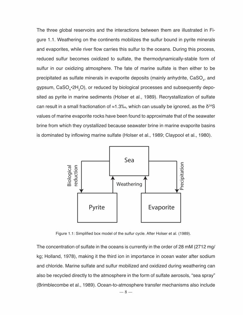
The three global reservoirs and the interactions between them are illustrated in Fi-
gure 1.1. Weathering on the continents mobilizes the sulfur bound in pyrite minerals
and evaporites, while river flow carries this sulfur to the oceans. During this process,
reduced sulfur becomes oxidized to sulfate, the thermodynamically-stable form of
sulfur in our oxidizing atmosphere. The fate of marine sulfate is then either to be
precipitated as sulfate minerals in evaporite deposits (mainly anhydrite, CaSO4, and
gypsum, CaSO4•2H2O), or reduced by biological processes and subsequently depo-
sited as pyrite in marine sediments (Holser et al., 1989). Recrystallization of sulfate
can result in a small fractionation of ≈1.3‰, which can usually be ignored, as the δ34S
values of marine evaporite rocks have been found to approximate that of the seawater
brine from which they crystallized because seawater brine in marine evaporite basins
is dominated by inflowing marine sulfate (Holser et al., 1989; Claypool et al., 1980).
Sea
Pyrite Evaporite
Biol
ogic
alre
duct
ion
Prec
ipita
tion
Weathering
Figure 1.1: Simplified box model of the sulfur cycle. After Holser et al. (1989).
The concentration of sulfate in the oceans is currently in the order of 28 mM (2712 mg/
kg; Holland, 1978), making it the third ion in importance in ocean water after sodium
and chloride. Marine sulfate and sulfur mobilized and oxidized during weathering can
also be recycled directly to the atmosphere in the form of sulfate aerosols, “sea spray”
(Brimblecombe et al., 1989). Ocean-to-atmosphere transfer mechanisms also include

— 9 —
the production of biogenic gases, volcanic eruptions and the release of S compounds
at hydrothermal vents. Without the current anthropogenic input to the sulfur cycle, with
anthropogenic S emissions at present accounting for approximately 55% of the total
sulfur input to the continental atmosphere (Brimblecombe et al., 1989), net transport
of sulfur would occur from sea to land (Brimblecombe et al., 1989; Schlesinger, 1991).
Two major aspects of the global sulfur cycle will be considered here in greater detail:
these are microbial cycling (Section 1.2.1) and atmospheric cycling (Section 1.2.2).
1.2.1 Microbial cycling of sulfur
Sulfur is required by living systems and can be found in a wide variety of compounds,
only few of which are considered to be necessary for normal cell function. Some ex-
amples are the amino acids cysteine and methionine, glutathione, thiamine, vitamin B,
biotin, ferrodoxin, lipoic acid, and coenzyme A (Krouse et al., 1991). Sulfur constitutes
on average ≈1% of the dry mass of living organisms and is mainly found in its reduced
state (-2), while accessible sulfur in the planet’s oxidizing environment is found mostly
in its oxidized form (+6). This entails that organisms must first reduce sulfur before it
can be incorporated into cellular organic compounds. This is accomplished via assimi-
latory sulfate reduction, a metabolic pathway that represents an overall loss of energy,
in contrast to dissimilatory sulfate reduction, which is an energy-yielding process.
The biological dissimilatory sulfate reduction of sulfate to sulfur, a key step in the
global sulfur cycle, is carried out by anaerobic sulfate-reducing bacteria (Roy and
Trudinger, 1970) and one group of archaea (Shen and Buick, 2004). The overall reac-
tion for microbial sulfate reduction (MSR) can be expressed as:
SO42- + CH2O S2- + CO2 + 2H2O
where CH2O represents any degradable organic carbon and S2- represents any com-
pletely reduced sulfide (Holser et al., 1989). This process can be thought of in terms of
— 10 —
a process similar to denitrification, with the SO42- acting as an alternative electron ac-
ceptor during the oxidation of organic matter. The term “dissimilatory” implies that the
sulfate is not used as a nutrient by the microbes carrying out the reaction, but rather
as a means of obtaining the necessary energy for metabolic functions. From this point
on, the expression “sulfate reduction” will be used solely to refer to the metabolism
dissimilatory sulfate reduction.
In coastal marine sediments, the importance of bacterial sulfate reduction is such that
it is estimated to account for more than 50% of the total carbon mineralization on the
ocean floor (Jørgensen, 1982; Canfield, 1993). MSR has an influence on the pyrite
content of sedimentary rocks and the fate of organic matter in sedimentary basins,
and thus ultimately on the redox conditions of the atmosphere, hydrosphere and litho-
sphere. Without MSR, some types of mineral deposits would not form and the mineral
assemblage landscape would be dramatically different.
1.2.1.1 Antiquity of microbial sulfate reduction
Sulfate reducers are widely distributed in anaerobic terrestrial and oceanic environ-
ments and, as a group, can withstand a wide range of ecological conditions, from very
cold (e.g., Isaksen and Jørgensen, 1996) to very hot (e.g., Jørgensen et al., 1992).
Sulfate reducers are also phylogenetically diverse, with some groups branching very
early in the Tree of Life (e.g., Stackebrandt et al., 1995) and perhaps representing
some of the very earliest life forms to have appeared on Earth, as the early Archaean
oceans would have been dominated by anaerobic microbes (Knauth, 2005). Thus,
understanding how the sulfate reduction metabolism evolved, and how it functions,
can help us understand the conditions prevailing on early Earth.
Evidence of early sulfate reduction is found mostly in the form of characteristic sulfur
stable isotope signatures in rocks and sediments, as molecular markers of sulfate
— 11 —
reduction do not survive geological conditions in any recognizable form, and fossils of
early sulfate-reducers would not be morphologically-distinct enough to tell apart from
those of other microorganisms (Shen and Buick, 2004). During MSR, the reactant sul-
fate is depleted in the lighter isotope of sulfur 32S (and enriched in the heavier isotope 34S), while the product sulfide is enriched in 32S (and depleted in 34S). Similar levels of
fractionation as those resulting from MSR can be accomplished through the abiologi-
cal reduction of sulfates, termed “thermochemical sulfate reduction”, but this process
is understood to take place only at high temperatures (80-100°C < T < 150-200°C),
beyond those in which sulfate reducers are able to metabolize (Machel et al., 1995).
As a result, significant depletions of sedimentary sulfides in 34S relative to coeval sul-
fate from low-temperature deposits are a powerful proxy for the involvement of micro-
bial sulfate reduction in sulfur cycling.
Currently, MSR is known to be accomplished by five phylogenitically-distinct groups of
microbes: archaea of the genus Archaeoglobus (hyperthermophilic: >70°C), the hy-
perthermophilic genus of bacteria Thermodesulfobacterium, the genus Thermodesul-
fovibrio of the Nitrospirae phylum (thermophilic: 40‐70°C), the genera Desulfotomacu-
lum and Desulfosporosinus of the Firmicutes, and several genera of Proteobacteria,
including the thermophilic genus Thermodesulforhabdus and several mesophilic
(15‐45°C) genera, including the common genus Desulfovibrio (Shen and Buick, 2004).
Leaving aside some of the complicating effects of mass-independent fractionation
(Farquhar et al., 2008), some of the oldest terrestrial S-isotopic records suggestive of
MSR have been found in the banded iron formations of the Isua supracrustal rocks
of West Greenland (>3.7 Ga; Monster et al., 1979) and show the narrow range of
δ34S values characteristic of rocks of Archaean age (e.g., Anbar and Knoll, 2002). In
sedimentary sulfides younger than 2.8 Ga, however, for example in those of the Mich-
ipicoten and Woman River Iron formations of Canada (Goodwin et al., 1976), sulfide
— 12 —
δ34S values are distinctly shifted towards negative values, with fractionation relative
to coeval sulfates in the order of the tens of per mil (e.g., Kakegawa et al., 1999;
Grassineau et al., 2000). This has been interpreted as strong evidence that MSR had
evolved by 2.7 Ga. Large fractionations (40-45‰), which are typical of MSR in non-
limiting sulfate conditions, (Shen and Buick, 2004) are found in the rock record from
2.3 Ga and could indicate an increase in oceanic sulfate concentrations resulting from
increased atmospheric oxygen content (Cameron, 1982). This record of large frac-
tionations extends continuously from 1.0 Ga, suggesting that today’s complex modern
sulfur cycle was fully established by this time (Canfield and Teske, 1996) [Figure 2].
The low S fractionations recorded in ancient Archaean rocks have been attributed to
either MSR in limiting sulfate conditions, implying that the oceans had not yet fully
oxygenated, or to sulfides of abiological origin, implying that MSR had not yet evolved
(Cameron, 1982; Walker and Brimblecombe, 1985; Habicht et al., 2002; Canfield et
al., 2000). Before the establishment of the oxygenic weathering cycle (≈2 Ga), sulfate
could be provided in small amounts by volcanic activity, through the oxidation of vol-
canic and volcanogenic sulfur gases (Perry et al., 1971; Walker and Brimblecombe,
1985). An alternate hypothesis has been put forth and maintains that atmospheric ox-
ygen reached present-day levels by 3.8 Ga, its presence persisting until now (Ohmoto
et al., 1993; Ohmoto, 1997), but our current understanding of isotopic fractionation
during MSR does not appear to support this view (e.g., Shen and Buick, 2004). If
the modern ocean is rich in sulfates, sulfate concentrations in the Archaean oceans
were probably very low, increasing with the rise of oxygenic photosynthesis, but likely
remaining below 1 mM levels until ≈2.3 Ga (Canfield and Raiswell, 1999). Some Ar-
chaean environments may have been sulfate-rich, as indicated by the precipitation
of evaporitic sulfate minerals (e.g., Buick and Dunlop, 1990). These sulfates may
have originated from the anoxygenic phototrophic oxidation of mantle-derived sulfide
(Canfield and Raiswell, 1999) or the hydrolysis of volcanogenic SO2 from relatively
— 13 —
oxidized magmas (Hattori and Cameron, 1986).
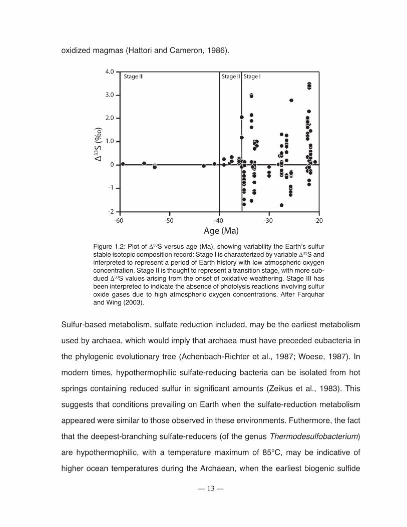
Figure 1.2: Plot of Δ33S versus age (Ma), showing variability the Earth’s sulfur stable isotopic composition record: Stage I is characterized by variable Δ33S and interpreted to represent a period of Earth history with low atmospheric oxygen concentration. Stage II is thought to represent a transition stage, with more sub-dued Δ33S values arising from the onset of oxidative weathering. Stage III has been interpreted to indicate the absence of photolysis reactions involving sulfur oxide gases due to high atmospheric oxygen concentrations. After Farquhar and Wing (2003).
Sulfur-based metabolism, sulfate reduction included, may be the earliest metabolism
used by archaea, which would imply that archaea must have preceded eubacteria in
the phylogenic evolutionary tree (Achenbach-Richter et al., 1987; Woese, 1987). In
modern times, hypothermophilic sulfate-reducing bacteria can be isolated from hot
springs containing reduced sulfur in significant amounts (Zeikus et al., 1983). This
suggests that conditions prevailing on Earth when the sulfate-reduction metabolism
appeared were similar to those observed in these environments. Futhermore, the fact
that the deepest-branching sulfate-reducers (of the genus Thermodesulfobacterium)
are hypothermophilic, with a temperature maximum of 85°C, may be indicative of
higher ocean temperatures during the Archaean, when the earliest biogenic sulfide
4.0
3.0
2.0
1.0
0
-1
-2-60 -50 -40 -30 -20
Δ33
S (‰
)
Stage III Stage II Stage I
Age (Ma)
— 14 —
deposits could have formed (Stackebrandt et al., 1995). Recent sulfur isotopic data
from barite deposits in North Pole, Australia, indeed suggest that sulfate-reducers can
be traced back to ≈3.5 Ga (Shen et al., 2001), but whether the small fractionations
observed in these early Archaean deposits are indeed indication of biological implica-
tion remains controversial.
1.2.1.2 Microbial sulfate reduction metabolism
The metabolism of microbial sulfate reduction has been extensively studied over the
last several decades, with fractionation experiments conducted as early as in the
1950s (e.g., Thode et al., 1951; Harrison and Thode, 1958). Early models of the MSR
metabolism assumed that the reactions involved in the reduction of sulfate to sulfide
were first-order with respect to the concentration of sulfur species (e.g., Harrison and
Thode, 1958). The later Rees model (Rees, 1973), however, used zero‐order kinetics
to explain the isotopic fractionation of sulfur stable isotopes during sulfate reduction
by Desulfovibrio desulfuricans. More recent studies have expanded on this model and
revised the expected sulfur fractionation thresholds associated to MSR (Brunner and
Bernasconi, 2005; Brunner et al., 2005). These are discussed below.
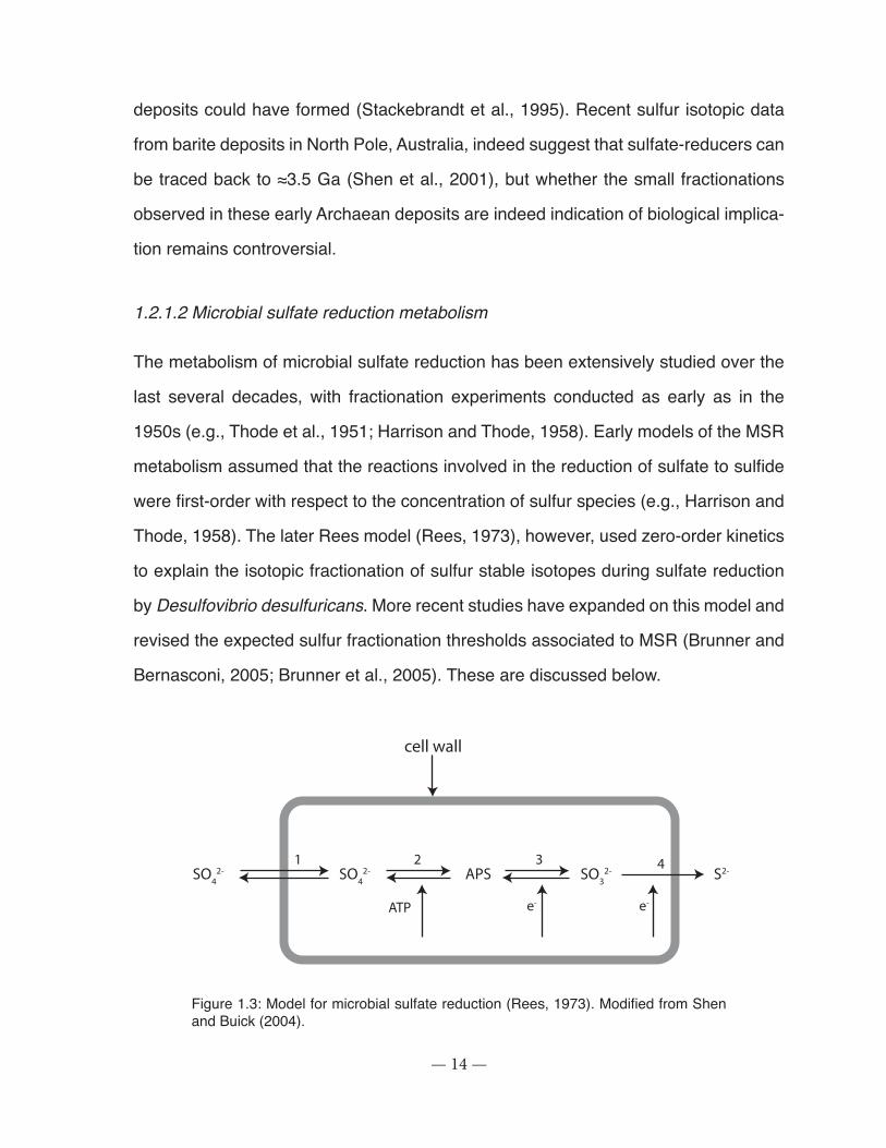
Figure 1.3: Model for microbial sulfate reduction (Rees, 1973). Modified from Shen and Buick (2004).
cell wall
SO42- SO4
2- SO32- S2-APS
ATP e- e-
1 2 3 4
— 15 —
In the Rees (1973) model, the first step (step 1, Figure 1.3) of the obligately anae-
robic sulfate reduction metabolism is the active uptake of the sulfate ion across the
cell wall. This fully reversible step (Cypionka, 1989; Warthmann and Cypionka, 1990;
Kreke and Cypionka, 1995) occurs via an electroneutral proton-anion symport driven
by the pH gradient across the membrane (Cypionka, 1987). It has been shown that in
the absence of a natural proton gradient, the entry of sulfate into the cell is severely
limited, but some strains are apparently able to self-generate such a gradient by pum-
ping protons across the cytoplasmic membrane (Fitz and Cypionka, 1989). The strain
Desulfovibrio vulgaris, for example, has been shown to generate a proton gradient by
vectorial proton translocation across the cytoplasmic membrane and by extracellular
proton release, this via a periplasmic hydrogenase enzyme (Fitz and Cypionka, 1991).
For most freshwater species, sulfate is taken up in the form of undissociated sulfuric
acid, while for marine species, protons are replaced by sodium ions to balance the
negative charge of sulfate (Cypionka, 1987; 1989; Warthmann and Cypionka, 1990;
Stahlmann et al., 1991). Once the sulfate ion has entered the cell, it reacts with ade-
nosine triphosphate (ATP) to form adenosine‐5’‐phosphosulfate (APS) ‐ the enzyme
ATP sulfurylase is involved in this activation step (step 2). The reduction of APS to
sulfite (step 3) is then catalyzed by the enzyme APS reductase. The final reduction of
sulfite to sulfide is mediated by the enzyme sulfite reductase (step 4). It is yet unclear
whether this last step involves a single, direct, 6-electron reduction mechanism, or
whether sulpihte is reduced via intermediate (thiosulfate and trithionate) compounds
(Kobayashi et al., 1974; Chambers and Trudinger 1975; Fitz and Cypionka, 1989;
1990; Brunner and Bernasconi, 2005). The reduced sulfide sulfur exits the cell through
passive diffusion in the form of hydrogen sulfide (step 4). At least in the case of the
2H+/SO42- symport found in freshwater species, this results in an overall electroneutral
cellular uptake mechanism, with two protons entering the cell during the uptake step
and two protons exiting the cell with the reduced sulfur (Cypionka, 1987).
— 16 —
The ability of sulfate-reducing microorganisms to accumulate internal sulfate to
concentrations far exceeding those in the outside environment has been clearly de-
monstrated. This process results in alkalinization of the growth medium without sulfide
production, and can lead to up to several thousand-fold sulfate accumulations (e.g.,
Cypionka, 1987; 1989). Experiments suggest that sulfate accumulation is greatest
after growth in sulfate-limiting conditions (Warthmann and Cypionka, 1990) and that
it is a function of the transmembrane proton gradient, thus becoming severely inhi-
bited at high pH, perhaps as a result of the disappearance of a natural proton gradient
between the environment and the cytoplasm (Cypionka, 1989). There is evidence
that at least some strains of sulfate-reducing microbes possess two distinct sulfate
accumulation mechanisms, each with different energy requirements (Cypionka, 1989;
Warthmann and Cypionka, 1990): a low-accumulation system with 3H+ taken for every
sulfate anion would be used at high sulfate concentrations, regulated to avoid unne-
cessary energy-spoiling accumulation, while a high-affinity accumulation system with
2H+ per sulfate anion would be favoured in sulfate-limiting conditions. The latter may
represent a survival mechanism developed in response to prolonged exposure to low
sulfate concentrations (Warthmann and Cypionka, 1990; Kreke and Cypionka, 1992).
Isotopes effects during the microbial reduction of sulfate to sulfide arise from the reac-
tions that involve the breaking of S‐O bonds, thus from steps 3 (the conversion of APS
to sulfite), and 4 (the reduction of sulfite to sulfide) in the Rees model (Figure 1.3).
An approximate value of a 25‰ depletion in 34S relative to the source of sulfate was
originally assigned to each of these steps, while sulfate uptake was associated to
a reverse effect, with enrichment in 34S by 3‰ (Rees, 1973). This assumption was
based on the hypothesis that the isotope effects associated with the backward reac-
tion of steps 3 and 4 are close to zero because they involve the oxidation of sulfur
or reactions where the oxidation state of sulfur is not changed. The inverse isotope
effect for the uptake of the sulfate ion into the cell was explained by the favouring of
— 17 —
the sulfate ion with 34S compared to 32S. Restrictions to the validity of the Rees model
included the following: 1) the uptake of sulfate is independent of sulfate concentration
at high sulfate concentrations, 2) the flow between the external sulfate and the internal
sulfite is reversible, 3) measurements of isotope effects are made when the bacterium
is operating in the steady‐state regime to allow sulfate concentrations to reach limi-
ting conditions, and 4) the hydrogen sulfide product is sampled when the system has
reached steady‐state. The results of the studies presented in Chapter 3 suggest that
the uptake of sulfur inside the cell is indeed associated to low fractionation, but that
its direction is the same as that of subsequent metabolic steps (preferential uptake of
light sulfur).
A perceived short-coming of the Rees model has been that the maximum level of
fractionation it allows (≈46‰) fails to explain the discrepancy with modern microbial
sulfide deposits (70‰). A later model (Brunner and Bernasconi, 2005) suggested that
these larger fractionations could indicate the alternate pathway proposed by Rees
(1973) in the sulfate reduction metabolism, one that would see the sulfite‐to‐sulfide
reduction taking place in multiple steps instead of a single 6-electron step. Studies
conducted using 35S‐labelling support the single‐step theory (Chambers and Trudin-
ger, 1975), but others show that intermediates such as thiosulfate and trithionate can
be produced (e.g., Kobayashi et al., 1974; Fitz and Cypionka, 1990). A revised ver-
sion of the Rees model (Brunner and Bernasconi, 2005) holds that intermediates are
indeed formed during the reduction of sulfite to sulfide (step 3). The proposed trithio-
nate pathway involves three reactions: 1) the formation of trithionate from three sulfite
molecules, a step mediated by the enzyme sulfate reductase, 2) the formation of thio-
sulfate and sulfite by the enzyme trithionate reductase, and 3) the formation of sulfide
and sulfite by thiosulfate reductase (Cypionka, 1995). This revised model suggests
that the maximum isotopic fractionation associated to steps 3 and 4 as defined by
Rees (1973) [Figure 1.3] represents the minimum fractionation possible rather than
— 18 —
the maximum. Thus, the theoretical maximum for sulfur isotopic fractionation during
microbial sulfate reduction should be revised to approximately 70‰, in accordance
with the maximum observed in modern sulfide deposits (Brunner and Bernasconi,
2005), instead of the upper limit of 46‰ proposed by Rees (1973) and reproduced in
laboratory experiments. Before the publication of the results of a recent study that de-
monstrated the possibility of >46‰ fractionations in laboratory conditions (Sim et al.,
2011), it had been hypothesized that the full range of isotopic fractionation required
combined hypersulfidic and substrate‐limiting conditions at a non‐limiting supply of
sulfate (Wortmann et al., 2001; Brunner and Bernasconi, 2005), or additional fractio-
nation during the extracellular oxidative sulfur cycle (Canfield and Thamdrup, 1994). A
possible alternate explanation for the previous absence of high fractionations in labo-
ratory experiments is that the sulfate reduction pathway must be operating in a highly
reversible manner in order for the full isotope effects to be expressed, a condition that
approaches equilibrium conditions between sulfate and sulfide and is thus difficult to
attain (Sim et al., 2011; Brunner and Bernasconi, 2005).
1.2.1.3 Sources of sulfur fractionation during microbial sulfate reduction
A number of biological, chemical and physical variables have been found to influence
the extent of kinetic fractionation processes taking place during MSR and in the past
few decades, an impressive body of research has been dedicated to studying, either
in natural settings or in laboratory conditions, the effect of these environmental factors
on S isotope fractionation. These variations as a function of environmental conditions
arise from biological, chemical, and physical factors, and are discussed below.
1.2.1.3.1 Biological factors
Biological factors known to affect sulfur fractionation during MSR include phylogeny
(genetic differences between species), enzymatic differences, and carbon oxidation
— 19 —
pathway. Phylogeny may play a role in the fractionation of S-isotopes during bacte-
rial sulfate reduction insofar as it reflects different metabolic characteristics (Brüchert
et al., 2001) and thus physiological differences (Widdel and Hansen, 1992). These
may include differences in cell membrane composition, structural differences between
APS and dissimilatory sulfite reductase enzymes, the use of different enzymes in the
electron transport chain, and varying capacity in terms of substrate use (Hansen,
1994). Genetic evidence for the existence of different APS reductases and dissimila-
tory sulfite reductases in sulfate-reducing bacteria has been uncovered (Minz et al.,
1999; Wagner et al., 1998) and different strains of sulfate-reducing bacteria may pos-
sess different cytochromes for the regulation of the electron flow from the organic
substrate (Hansen, 1994). Enzymes with different structures would be expected to
possess different activation energies, which may in turn influence the isotopic frac-
tionation associated to each step in the sulfate-reduction metabolism (Brüchert et al.,
2001). Additionally, the carbon oxidation pathway used for the oxidation of organic
substrate during bacterial sulfate reduction may play a role in the fractionation of S
isotopes, with its influence potentially related to the energy yield associated to the
organic substrate used (see Section 1.2.1.3.2).
The microbial metabolism of a given substrate can involve complete or incomplete ox-
idation. Acetate is a common product of the incomplete oxidation of some fatty acids
whereas complete oxidation yields CO2 as a product (Hansen, 1994). The term “com-
plete oxidizer” is generally used to refer to sulfate reducers that are able to oxidize
the C2-unit of acetyl-CoA to CO2, but acetate can nevertheless be excreted in consid-
erable amounts during growth (Hansen, 1994). Differences in fractionation between
pathways can be rationalised in terms of the energy conserved during the oxidation
of the organic substrate: more energy is conserved per mole of sulfate for incomplete
oxidation compared to complete oxidation (Detmers et al., 2001). For example, com-
plete oxidation of acetate to CO2 yields three times less energy than the incomplete
— 20 —
oxidation of lactate to acetate (Detmers et al., 2001). An extensive study of 32 strains
of sulfate-reducing microbes showed that while all strains discriminated against 34S,
the largest fractionations were observed with complete oxidizers, which fractionated
between 15.0‰ and 42.0‰, while for the acetate-excreting incomplete oxidizers frac-
tionations were between 2.0‰ and 18.7‰ (Detmers et al., 2001). In a similar study, it
was found that complete oxidizing strains fractionated sulfur to a greater extent (13-
22‰) than incomplete oxidizing strains (4.6-10‰) [Brüchert et al., 2001].
The nature of the substrate used for MSR also appears to have an effect on the extent
of fractionation with, for example, MSR using lactate rather than acetate leading to
smaller fractionations (Brüchert et al., 2001).
Very few studies have investigated the role played by enzymes involved in the sul-
fate reduction metabolism and its subsequent influence on the extent of fractionation.
However, the role of the enzyme dissimilatory sulfite reductase, which mediates the
last reduction step of APS to sulfite, has been investigated in experiments where ni-
trite – an inhibitor of this enzyme – was added. The results indicate that sulfate reduc-
tion is in part regulated by kinetic conversions during the metabolism: without nitrite
to inhibit the enzyme’s activity, fractionation is low, indicating fast sulfite-to-sulfide
reduction, but with nitrite, the reaction rate associated to the enzyme becomes the
rate-limiting step (Mangalo et al., 2008; Brunner and Bernasconi, 2005).
1.2.1.3.2 Chemical factors
Type of electron donor - substrate type
As a group, sulfate-reducers are very versatile in the variety of electron donors they
can couple to the reduction of sulfate. At least 125 compounds have been identified
as usable electron donors in studies using pure cultures of sulfate reducers (Hansen,
1993), most of which are typical fermentation products and intermediate metabolic
— 21 —
compounds, such as amino acids, fatty acids, and glycerol. This versatility likely stems
from the necessity, in natural environments, to adapt to varying conditions in substrate
composition and availability. Although acetate and lactate are most frequently used for
bacterial growth in microcosm experiments, a variety of other fatty acids can serve as
electron donors. For example, low molecular weight fatty acids appear to be the pre-
ferred substrate in saline sediments (acetate, butyrate and propionate, together with
hydrogen; Sørensen et al., 1981), perhaps because they are natural products of the
anaerobic fermentation of organic matter in natural environments (Trudinger, 1992).
Ethanol and a number of petroleum hydrocarbons have also been used successfully
as a source of carbon in laboratory experiments. Growth using organic matter as the
electron donor is heterotrophic, but some sulfate reducers can grow autotrophically
using H2.
An effect of carbon substrate type on sulfur stable isotope fractionation would be
expected from its relationship with sulfate reduction rates (Kaplan and Rittenberg,
1964; Kemp and Thode, 1968), as these may depend on the quantity and quality of
the organic matter available for oxidation (Westrich and Berner, 1984). The oxidation
pathway - complete or incomplete - and the free energy change associated with the
oxidation of electron donors are also likely key factors in determining sulfate reduc-
tion rates, and by extension the extent of fractionation (Hansen, 1994; Widdel and
Hansen, 1992): more negative free energy changes tend to be associated to lower
fractionations (e.g., lower fractionations with lactate compared to acetate; Kaplan and
Rittenberg, 1964; Brüchert et al., 2001; Detmers et al., 2001) [Table 1]. Furthermore,
acetate, which is likely a key substrate in natural settings, has received relatively little
attention (Canfield, 2001). The underlying causes for the link between free energy
change and isotope fractionation remains unclear (Detmers et al., 2001), but there
is evidence that any electron donor effect on fractionation may not be due solely to
ensuing changes in sulfate reduction rates. The mechanism of sulfur isotope fraction-

— 22 —
ation remains unclear, and the relationship between substrate type and the extent
of fractionation is complex. Investigations at the enzymatic level may be necessary
to fully understand the mechanism of S isotope fractionation during bacterial sulfate
reduction.
Table 1.1: Free energy changes at standard state (ΔG0’) and corresponding range of isotope fractio-nations (ε) during dissimilatory sulfate reduction with various electron donors for complete and incom-plete oxidation (from Detmers et al., 2001).
Electron donor (type of oxidation) Stoichiometry
ΔG0’ (kJ mol-1
SO42-)
ε (‰)
Pyruvate (incomplete)
4CH3COCOO- + 4H2O + SO42- →
4CH3COO- + 4HCO3- + HS- + 3H+
-340.9 8.1
Lactate (incomplete)
2CH3CHOHCOO- + SO42- →
2CH3COO- +2HCO3- + HS- + H+
-160.1 2.0-17.0
Hydrogen 4H2 + SO42- +H- → 4H2O + HS- -152.2 14.0
Formate 4HCOO- + SO42- + H+ → 4HCO3
- + HS- -146.9 5.5Ethanol (incomplete)
2CH3CH2OH + SO42- → 2CH3COO- + HS- + 2H2O + H+ -146.6 18.7
Pyruvate (complete)
4CH3COCOO- + 4H2O + 5SO42- → 12HCO3
- +5 HS- + 3H+ -106.3 16.1; 25.7
Proprionate (imcomplete)
4CH3CH3COO- + 3SO42- →
4CH3COO- + 4HCO3- + 3HS- + H+-50.2 5.5; 6.8
Benzoate (complete)
C7H5O2- + 3.75SO4
2- + 4H2O → 7HCO3- + 3.75HS- + 2.25H+ -49.7 15.0-42.0
Butyrate (complete)
CH3CH2CH2COO- + 2.5SO42- → 4HCO3- + 2.5HS- + 0.5H+ -49.2 23.1-32.7
Acetate (complete)
CH3COO- + SO42- → 2HCO3- + HS- -47.6 18.0-22.0
A limited number of organic substrates have been investigated in both pure and en-
richment cultures of sulfate-reducing bacteria in comparison to the variability occurring
in natural environments and very few studies have investigated the effect of organic
substrate concentration on S isotope fractionation. In most studies investigating S-
isotope fractionation during bacterial sulfate reduction, organic substrate is provided
in excess. In natural environments, however, sulfate-reducers may experience or-
ganic substrate limitation (Isaksen et al., 1994; Sagemann et al., 1998). Experimental
evidence suggests that when an organic substrate becomes limiting, sulfur is increas-
ingly found in intermediate species (Cypionka, 1995), increasing the likelihood of back
— 23 —
reactions from intermediates to sulfite occurring, and effecting a change in isotope
fractionation (Chambers et al., 1975; Fitz and Cypionka, 1990). Substrate limitation,
combined with excess sulfate and hypersulfidic conditions, may explain some of the
fractionations in nature greater than the 46‰ value reported in most experiments with
pure cultures (Brunner and Bernasconi, 2005), although a recent study has shown
that these conditions are not necessary to generate larger fractionations (Sim et al.,
2011).
Sulfate availability
An obvious prerequisite of MSR is presence of sulfate in sufficient quantity, but sul-
fate reduction has been demonstrated to take place at even minute concentrations
of sulfate (<50 μM; e.g., Habicht et al., 2002). A consistent relationship has been
found between level of fractionation and sulfate concentration, this both in pure and
enrichment cultures. At low (limiting) sulfate concentrations, fractionations are gener-
ally small (<10‰; Habicht et al., 2002), while high fractionations (up to 50‰; Harrison
and Thode, 1958; Habicht & Canfield, 1996; Canfield et al., 2000; Canfield, 2001)
are reported at non-limiting concentrations. As a general rule, fractionation increases
with increasing sulfate concentration in sulfate-limiting conditions, but appears to be
uncorrelated to sulfate concentration in non-limiting conditions (e.g., Harrison and
Thode, 1957; Chambers et al., 1975; Kaplan and Rittenberg, 1964; Kemp and Thode,
1968; Habicht and Canfield, 1997; Canfield, 2001). A possible explanation for this ap-
parent first-order dependence of S-isotope fractionation on sulfate concentration is
that when sulfate becomes limiting, sulfate-reducers must actively pump sulfate into
the cell, which reduces the free exchange of sulfate in and out of the cell. The energy
increase associated to active uptake leads to a reduction in growth yield; to maintain
energy for growth, specific sulfate reduction rates are increased, which in turn leads
to lower fractionations (Habicht et al., 2005) as sulfate is processed rapidly within the

— 24 —
cell. There may also be a link with the high-accumulation mechanism of sulfate uptake
described in some strains of sulfate reducing bacteria (Kreke and Cypionka, 1992).
Environmental pH
Until recently, the vast majority of isolated strains of sulfate reducing bacteria were
neutrophilic (preferring pH 6-9) and it was thought that communities of sulfate-reduc-
ers in acidic environments (e.g., acid mine drainage environments) were not geneti-
cally diverse (Kolmert and Johnson, 2001). It is now recognized that the biodiversity of
these environments may be considerable (Johnson, 2000). If many bacteria species
in these environments are neutrophilic but acid-tolerant and thus able to survive and
metabolise at low pH, truly acidophilic strains would be expected to be present as
well. Recently, such bacteria have been isolated from acid mine drainage-impacted
sites and geothermal environments: grown in laboratory media, these were shown to
conduct sulfate reduction at pH values as low as 3 (Sen and Johnson, 1999; Senko et
al., 2009). Acidic waters often contain excess sulfate and dissolved metals. Addition-
ally, they are often-carbon limited (Koschorreck, 2008). As sulfate reduction is a pro-
ton-consuming reaction, the potential free energy associated to the reaction increases
with lower pH, creating an energetic advantage to sulfate reduction at low pH (Kos-
chorreck, 2008). Very few studies, if any, have investigated the effect of pH on isotope
fractionation during microbial sulfate reduction. In fact, most sulfate reduction studies
have investigated neutrophilic strains of sulfate-reducers at either near-neutral or opti-
mum pH values, and those that have attempted to investigate sulfate reduction at low
pH have not considered isotopic fractionation. Thus at the present time, information
on the effect of pH on the fractionation of sulfur stable isotopes during bacterial sul-
fate reduction is inadequate. Considering the acidic and reducing conditions that are
thought to have prevailed during the Archaean, investigating sulfur fractionation by
acidophilic or acidotolerant strains of sulfate-reducers at low pH may help understand
— 25 —
the large range of sulfur fractionation observed in biogenic sulfide deposits. There is
evidence that cells can accumulate sulfate internally in concentrations significantly
higher than those present in the environment and that at least some sulfate reducers
possess two distinct accumulation systems (e.g., Warthmann and Cypionka, 1990;
Kreke and Cypionka, 1992), which could play a role in determining the overall fraction-
ation of sulfur between the sulfate and sulfide fractions. Chapter 3 presents the results
of a series of experiments designed to investigate the fractionation of sulfur isotopes
during MSR by two strains of acid-tolerant sulfate reducers. One goal of the study was
to determine whether pH exerts an an effect on the level of fractionation taking place
during MSR. Additional objectives were to determine the level of fractionation associ-
ated to MSR by acid-tolerant sulfate-reducing bacteria.
1.2.1.3.3 Physical factors
Sulfate reduction rate
There is evidence suggesting that a link between sulfate reduction rates and sulfur
isotope fractionation exists. This inverse relationship of fractionation increasing as
sulfate reduction rates decrease - and vice versa - has been reported in a number of
earlier studies (Harrison and Thode, 1958; Kaplan and Rittenberg, 1964; Chambers
et al., 1975) as well as in recent publications (Habicht and Canfield, 1997; Canfield,
2001; Brüchert et al., 2001). However, detailed studies of S-isotope fractionation over
a wide range of sulfate reduction rates found no correlation between fractionation and
reduction rate (Canfield and Teske, 1996; Rudnicki et al., 2001; Farquhar et al., 2008).
It has been suggested that when sulfate reducers are grown in optimal conditions,
isotope fractionation is independent of sulfate reduction rates (Bolliger et al., 2001;
Detmers et al., 2001). Phylogenetic differences may play a more important role than
sulfate reduction rate in determining the level of sulfur fractionation (Brüchert et al.,
2001).

— 26 —
Sulfate reduction rates may also depend on the concentration of dissolved sulfate, but
experiments suggest that the rate of sulfate reduction is independent of the concen-
tration of dissolved sulfate until low concentrations (< 3 mM) are reached (Boudreau
and Westrich, 1984; Ingvorsen et al., 1984; Ingvorsen and Jørgensen, 1984; Habicht
et al., 2002). A link between sulfate reduction rate and temperature has also been
suggested, although sulfate reduction signatures appear to deviate from equilibrium
considerations, suggesting that they are independent of temperature (Johnston et
al., 2007) within an organism’s tolerance range. The apparent inverse relationship
between isotope fractionation and sulfate reduction observed may arise from the influ-
ence of the specific sulfate-reduction rate on the exchange of sulfate across the cell
membrane, and on the reversibility of each step in the metabolism of sulfate reduction
(Canfield, 2001). As such, the extent of isotope fractionation rate may be correlated
with the specific rate of sulfate reduction, but not the absolute rate, which may serve
to explain discrepancies in reported results. Cell-specific rates of sulfate reduction
(csSRR) are calculated as a function of cell density, and are represented by dividing
the sulfate reduction rate by the cell density in the culture. Specific rates of sulfate
reduction are more easily obtained in controlled growth media.
Temperature
Temperature has the potential to influence S-isotope fractionation through its effect
on membrane fluidity and its impact on the uptake of sulfate into the cell. At low
temperatures, cell membrane fluidity may be reduced (Scherer and Neuhaus, 2002),
leading to small fractionations (e.g., Kaplan and Rittenberg, 1964; Rees, 1973) result-
ing from reduced sulfate transport across the membrane. Higher temperatures within
the organism’s tolerance limit would likely facilitate sulfate transport by increasing
membrane fluidity, and if sulfate concentrations are low, then sulfate transport across
the membrane could become rate-limiting. Because only little fractionation is associ-
— 27 —
ated with this step (Rees, 1973; Chapter 3), the full extent of fractionation for subse-
quent steps in MSR would not be expressed and small overall fractionation would be
expected. Temperatures exceeding optimal growth conditions may lead to reduced
sulfate reduction rates due to damage to cell membranes and/or enzymes (Brüchert
et al., 2001). These mechanisms would predict low fractionation at low and high tem-
peratures, and high fractionation in the intermediate temperature range (Kaplan and
Rittenberg, 1964). An influence of temperature on the extent of fractionation not nec-
essarily following this model has been uncovered in a number of studies for some
strains and some substrates (Habicht and Canfield, 1997; Brüchert et al., 2001; Can-
field, 2001). However, other studies have found no consistent link between tempera-
ture and fractionation (Brüchert et al., 2001; Canfield, 2001; Rudnicki et al., 2001),
suggesting that in natural populations at least, varying fractionation levels within a
given microbial community may result more from differences between strains and
optimal temperatures for MSR rather than a temperature effect. In pure cultures, the
influence of temperature on fractionation may be dependent upon the exchange path
for the reduction of sulfate to sulfide, more specifically: 1) the rate of sulfate transport
in and out of the cell, and 2) the exchange of sulfur between sulfur pools internal to
the organism, with different sulfate reducing populations balancing the importance of
these two paths differently (Canfield et al., 2006). Possible confounding effects - both
biological and chemical - may be at play.
1.2.1.4 Distinguishing between sulfur isotope signatures from multiple microbial meta-
bolisms
By its significant (>50%) contribution to sedimentary organic matter respiration (Jør-
gensen, 1982), the microbial sulfate reduction metabolism was likely the major in-
fluence on the sulfur isotopic composition of biogenic sulfides throughout the planet’s
history. However, the microbial cycling of sulfur is accomplished via a variety of meta-
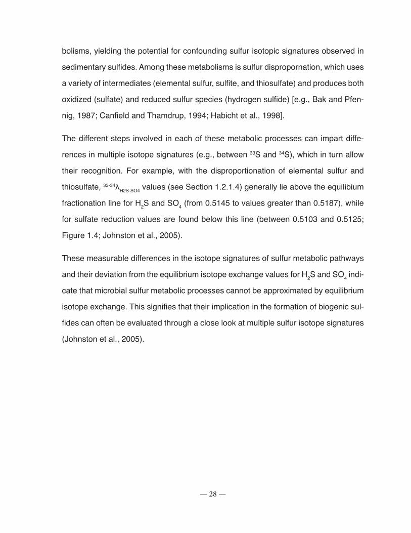
— 28 —
bolisms, yielding the potential for confounding sulfur isotopic signatures observed in
sedimentary sulfides. Among these metabolisms is sulfur dispropornation, which uses
a variety of intermediates (elemental sulfur, sulfite, and thiosulfate) and produces both
oxidized (sulfate) and reduced sulfur species (hydrogen sulfide) [e.g., Bak and Pfen-
nig, 1987; Canfield and Thamdrup, 1994; Habicht et al., 1998].
The different steps involved in each of these metabolic processes can impart diffe-
rences in multiple isotope signatures (e.g., between 33S and 34S), which in turn allow
their recognition. For example, with the disproportionation of elemental sulfur and
thiosulfate, 33-34λH2S-SO4 values (see Section 1.2.1.4) generally lie above the equilibium
fractionation line for H2S and SO4 (from 0.5145 to values greater than 0.5187), while
for sulfate reduction values are found below this line (between 0.5103 and 0.5125;
Figure 1.4; Johnston et al., 2005).
These measurable differences in the isotope signatures of sulfur metabolic pathways
and their deviation from the equilibrium isotope exchange values for H2S and SO4 indi-
cate that microbial sulfur metabolic processes cannot be approximated by equilibrium
isotope exchange. This signifies that their implication in the formation of biogenic sul-
fides can often be evaluated through a close look at multiple sulfur isotope signatures
(Johnston et al., 2005).
— 29 —
Bulk disproportionation
Equilibrium fractionation line
Bulk dissimilatory sulfate reduction
0.519
0.517
0.515
0.513
0.511
0.509
0.507
0.505-60 -50 -40 -30 -20 -10
λ H
2S-S
O4
δ34S’ - δ34S’ H2S SO4
Figure 1.4: Plot of λH2S-SO4 versus δ34S’H2S-δ34S’SO4 from experiments with sulfate reducing microbes. The gray line represents equilibrium exchange between H2S and SO4 (from Johnston et al., 2005).
1.2.2 Atmospheric sulfur cycling
The atmosphere is a very mobile system in which most processes take place in no
more than a few days. Sulfur enters the atmosphere in gaseous or particulate form
from a variety of sources. The major natural fluxes influencing the global atmospheric
sulfur budget are: i) biogenic emissions from coastal regions, the open ocean and
land, ii) aeolian weathering of sulfates, iii) sea spray sulfate from the ocean, and
iv) volcanic exhalations. Sulfur compounds in the atmosphere can occur in the gas-
eous, liquid, and solid phases. Reduced species released into the planet’s oxidizing
atmosphere are initially oxidized to sulfur dioxide (SO2) and methane sulfonic acid
(CH3SO3H or “MSA”) [oxidation state +4], and ultimately to sulfuric acid (H2SO4, +6),
the thermodynamically stable form of sulfur in the presence of oxygen.
— 30 —
1.2.2.1 Input of sulfur compounds from the atmosphere
Biogenic sources of sulfur are estimated to constitute as much as 50% of the total
atmospheric sulfur burden (Kellogg et al., 1972; Ryaboshapko, 1983). Biogenic emis-
sions - largely produced by vegetation and anaerobic respiration processes in anoxic
environments - occur predominantly in the form of reduced sulfur. Plants can emit sul-
fur in the form of hydrogen sulfide (H2S), dimethylsulfide (CH3SCH3, “DMS”), carbonyl
sulfide (COS) and carbon disulfide (CS2) (Aneja and Cooper, 1989). Biologically-ac-
tive areas, for example sea marshes and the tidal flats of marine environments, serve
both as sources and sinks for a number of sulfur compounds, and so sulfur plays an
important role in biological processes in these environments, notably via oceanic sul-
fate, the major electron acceptor for respiration in anoxic sediments (Ingvorsen and
Jørgensen, 1982). In the oceans, DMS is produced by benthic and mostly planktonic
marine algae (Andreae and Barnard, 1984) and represents 50% of all biogenic gases
emitted to the atmosphere (Ferek et al., 1986). In the atmosphere, DMS forms sul-
fate aerosols, which in turn serve as a source of cloud-condensation nuclei over the
oceans, playing an important role in the regulation of the Earth’s climate (Charlson et
al., 1987; Cropp et al., 2005).
The second most important flux in the atmospheric component of the sulfur cycle is
the aeolian weathering of sulfates from the continental surface. This flux is difficult to
quantify and may vary greatly in time and space. Arid regions and areas where dust
storms are frequent may contribute the largest portion of aeolian sulfur material to the
atmosphere (Grinenko and Ivanov, 1983). At present, the contribution of this source
to the atmospheric sulfur budget is estimated at less than 6% of total S emissions
(Brimblecombe et al., 1989), but is thought to have increased significantly as a result
of human activities that increase erosion (Brimblecombe et al., 1989).
The contribution of sea spray sulfates (or sea salt sulfates) to the global sulfur budget
— 31 —
has been estimated to be in the order of 144 Tg (S), representing approximately 42%
of the total sulfur input to the atmosphere (Brimblecombe et al., 1989). Sulfate aero-
sols enter the atmosphere in the form of tiny droplets that have become airborne as
a result of the bursting of bubbles at the water surface (MacIntyre, 1974; Wu, 1981).
The salt left behind when the water evaporates from the bubbles crystallizes and
forms the seasalt aerosols, which crudely approximate the composition of seawater
(Glass and Matteson, 1973). Seaspray sulfates are found everywhere in the oceanic
atmosphere and along the coasts, but only a small proportion of the seawater sul-
fate passes over land (≈10%), and only in coastal locations (Moss, 1978; Whelpdale,
1992). Modern oceans are rich in sulfates (28 mM), with sulfate currently one of the
most abundant ions in seawater, and a major component of the alkalinity budget (Mo-
rel and Hering, 1993). Ancient oceans, however, including the Archaean ocean, were
probably sulfate-poor, with concentrations increasing with the development of oxy-
genic photosynthesis (Canfield and Raiswell, 1999). The oceanic sulfate concentra-
tion has varied significantly over time, with concentrations stabilizing at current levels
≈50 million years ago (Paytan et al., 1998).
Volcanic activity releases a number of compounds into the atmosphere (water vapour,
carbon dioxide, sulfur dioxide, hydrogen sulfide, hydrogen chloride, various sulfates,
some sulfur trioxide), as well as solid matter (ash, lava) [Kellogg et al., 1972; Robock
and Oppenheimer, 2003]. Reduced sulfur gases in the lower troposphere are typically
rained out or rapidly oxidized to sulfate to form sulfate (sulfuric acid) aerosols, which
affect the Earth’s radiative balance directly by scattering solar radiation and indirectly
by serving as cloud condensation nucleii, increasing cloud cover and albedo (Tex-
tor et al., 2003). Volcanic ash, when exposed to water, can also mobilize a range of
sulfate and halide compounds (Witham et al., 2005). Although most of the sulfur on
the Earth’s surface apparently originated from outgassing of deep crustal and mantle
regions, the contribution of volcanoes to the present sulfur budget is quite small, with

— 32 —
estimates as low as 2% (Nielsen, 1974). H2S is also emitted in significant amounts by
hydrothermal vents in the oceans (Brimblecombe et al., 1989).
1.2.2.2 Removal of sulfur compounds from the atmosphere
Sulfur compounds in the atmosphere can be brought back to the surface through
various mechanisms, including wet deposition (precipitation) and dry deposition (pro-
cesses that do not involve precipitation). In wet deposition processes, sulfur gases are
removed during uptake into raindrops within clouds (in-cloud scavenging), uptake into
raindrops as they are falling to the ground beneath the clouds (sub-cloud scavenging)
[Ryaboshapko, 1983], or through their adsorbtion onto frozen precipitation elements
(Whelpdale, 1992). Sulfate particles are efficient cloud condensation nuclei (CCN)
and can thus be incorporated into precipitation or scavenged by cloud droplets and
falling drops (Whelpdale, 1992). The efficiency of sulfur removal by wet deposition
processes depends on their form and on characteristics of precipitation (type, inten-
sity, duration, frequency). For aerosol particles with diameters between 0.1 and 1 μm,
the primary removal mechanism is thought to be precipitation scavenging (Brasseur
et al., 1999). Particles with diameters of 10 μm or more may be removed by gravita-
tional sedimentation. Smaller particles and gases are more efficiently brought back to
the surface by turbulent atmospheric motions. The actual uptake of these smaller par-
ticles may be accomplished by chemical reaction, dissolution, adsorption and other
mechanisms (Whelpdale, 1992).
The sulfur dioxide entering the atmosphere is mostly deposited locally via precipitation
and dryfall, with the remainder undergoing long range transport (Schlesinger, 1991).
Sulfur dioxide in the atmosphere can be oxidized in the gas phase, on the surface
of soil particles, and in the liquid phase of droplets in clouds and fog (Ryaboshapko,
1983). The dominant process is by far oxidation in the gas phase and is attributable
primarily to reaction with the OH radical to form sulfate (Cox and Sheppard, 1980).
— 33 —
The rate of SO2 oxidation through this process is highly variable due to OH concentra-
tions in the atmosphere varying with cloudiness, time of day, season and latitude (so-
lar radiation intensity). For example, in cold and dark conditions, SO2 is not efficiently
oxidized (Hobbs et al., 1991). The half-life of sulfur dioxide and sulfate in the lower
atmosphere is estimated at approximately 10 hours and 48 hours, respectively, with a
half-life for transformation of sulfur dioxide to sulfate of 60 hours (Prahm et al., 1975).
Removal of sulfate aerosols from the atmosphere occurs primarily via wet deposition
within a few days, but their stratospheric lifetime can range from months to years.
1.2.2.3 Sulfur isotope fractionation in the atmosphere
From modern studies, a broad distinction can be made between sulfur that has and
has not participated in the sedimentary cycle, with the latter showing a much wider
range of isotope values. Volcanic gases and rocks tend to have a relatively narrow
range of δ34S values, centred around 0‰ (e.g., Grinenko and Thode, 1970; Hoefs,
1997), but with a wider spread than those associated with sulfur of meteoritic or mag-
matic (basaltic) origin (e.g., Grinenko et al., 1970). However, as some volcanoes can
act as pumps for a variety of sources of sulfur compounds, the isotopic composition
of volcanic gases depends on the nature of the source material. The isotopic compo-
sition of magma-derived sulfides can range to 4-5‰ of the mantle value (Schneider,
1970). Sulfur compounds of biological origin display a large range of isotopic compo-
sitions, hence igneous rocks with isotopic compositions departing significantly from
0‰ can be said with some certainty to contain some component of sedimentary sulfur.
There appears to be minimal enrichment in 34S (1.5-2.6‰) between sulfate and its
source SO2 when the sulfate is formed in the combustion process or at high tempe-
ratures (Forrest et al., 1973; Nriagu and Coker, 1978), but marine sulfate aerosols
tend to have δ34S compositions that are somewhat lower than that of the source sul-
fate, potentially due to the contribution from the oxidation of biogenic sulfides (Van
— 34 —
Everdingen et al., 1982; 1985). For reduced volcanic species such as H2S, some
fractionation is predicted as a result of the oxidation process, but this fractionation is
smaller than predicted by equilibrium exchange between sulfur species: δ34S values
for H2SO4 fallout are similar to the precursor H2S, but ambient SO2 is ≈5‰ depleted in 34S (Newman et al., 1991). Sulfate aerosols collected at basaltic vents are enriched in 34S, with δ34S values ≈8‰ (Mather et al., 2006).
— 35 —
Chapter 2: The Cretaceous-Paleogene extinction event
The Cretaceous-Paleogene boundary (KPg) boundary1 marks a significant biological
turnover in our planet’s history ≈65.5 million years ago (Gradstein et al., 2004). Along
with the Permian-Triassic, Triassic-Jurassic, Late Devonian, and Ordovician-Silurian
extinction events, it is known as one of the “big five”: extinction events in the Phane-
rozoic that stand out against a background of continuous extinctions in our planet’s
history through their role in the disappearance of >50% of well-preserved genera and
perhaps more than 70% of their species (Sepkoski, 1996). Although the KPg event
is perhaps best known for having led to the extinction of all non-avian dinosaurs, it is
also associated with the disappearance of many other groups of species, including
ammonites (Kennedy, 1989; Marshall, 1995), belemnites (Iba et al., 2011), heteroheli-
cid planktic foraminifera (Keller, 1989; Molina et al., 1998), mosasaurs and sauropto-
rygians (marine reptiles; Russell, 1967; Motani, 2009; Polcyn and Bell, 2005), plants
(e.g., Tschudy and Tschudy, 1986; Nichols and Johnson, 2008), and insects (Laban-
deira et al., 2002). The KPg boundary is marked by a continuous bedding plane that is
apparently partly consists in debris and dust from a bolide collision with evaporitic and
carbonate rocks (Schulte et al., 2010). This bedding plane is referred to as the “KPg
boundary” or “boundary claystone” and can be found at sites worldwide.
Many causes to the extinctions have been proposed, including the explosion of a
supernova (Russell and Tucker, 1971), a comet shower (Carlisle, 1995), flood basalt
eruptions (e.g., Officer & Drake, 1985), an asteroid or large comet impact (Alvarez et
al., 1980; Smit and Hertogen, 1980; Prinn and Fegley, 1987), changes in oceanogra-
phic or climatic conditions (e.g., Tappan 1968; McLean, 1978; O’Keefe and Ahrens,
1. The KPg boundary was formerly known as the K/T or K-T (Cretaceous-Tertiary) boundary”. This usage has been abandonned since the Tertiary is no longer recognized as a valid chronostratigraphic descriptor by the International Commission on Stratigraphy.
— 36 —
1989), a magnetic reversal (Simpson, 1966), and an arctic lake flooding the ocean
surface with freshwater (Gartner and Keany, 1978). With the finding of an iridium en-
richment in the boundary layer (Alvarez et al., 1980) and the subsequent discovery of
the Chicxulub structure (Hildebrand et al., 1991), followed by decades of extensive re-
search, the impact model has garnered significant support from the scientific commu-
nity (e.g., Schulte et al., 2010). This stems from overwhelming evidence for an impact
event at the end of the Cretaceous and its stratigraphic coincidence with the abrupt
disappearance from the fossil record of entire groups of species. KPg boundary sites
around the world feature direct evidence of an impact coeval with the emplacement
of the boundary claystone (tektites, shocked quartz) and indirect evidence that can
easily be reconciled with a rapid and catastrophic process with global consequences
(Section 2.3).
In their seminal paper, Alvarez et al. (1980) hypothesized that the mechanism of ex-
tinction at the boundary was the blocking of sunlight at the Earth’s surface by dust
and debris from a bolide impact, leading to the collapse of the food chain. The specific
mechanisms responsible for the biotic turnover, however, are still cause for debate
and have been thought to include other factors, including greenhouse-induced war-
ming (O’Keefe and Ahrens, 1989), wildfires (Wolbach et al., 1985), intense surface
heat and radiation (Melosh et al., 1990; Robertson et al., 2004), and ocean anoxia
(Kajiwara and Kaiho, 1992).
This chapter completes the information presented in Chapter 4. It includes a detailed
review of the nature of the boundary layer, an overview of the biotic impacts of the
KPg catastrophe, and some background information on the Deccan continental flood
basalts.
— 37 —
2.1 The Deccan continental flood basalts
The “Deccan Traps” are continental flood basalts that cover ≈500 000 km2 today,
but that may have originally covered up to one million square kilometers (Krishnan,
1960). The current thickness of the lava flows ranges from 2000 m in western India
to 100-200 m in central India (Bose, 1972). Continental flood basalts are a type of
large igneous province that erupt mostly subaerially, with the unique feature of being
characterized by the repeated eruption of large amounts of lava over short periods
of geologic time (Rampino and Stothers, 1988). Deccan volcanism is thought to have
originated from the passing of the Indian lithosphere over the deep mantle plume of
the Réunion hotspot, after the Indian plate became detached from Gondwanaland
(Morgan, 1972; Gupta and Gaur, 1984; Ganerød et al., 2011). Hot spot activity would
have bored through the lithosphere and extruded great volumes of tholeiitic basalts,
generating the structures know today as the Deccan traps.
The observation of modern eruptions associated with basaltic fissures (e.g., Laki vol-
cano, 1783 A.D.) hints at the formation of violent “fire fountains” during prolonged
flood basalt eruptions, reaching heights of up to 1.5 km (Thordarson and Self, 1998)
and perhaps 13 km at times in the case of convective plumes (Self et al., 2005). Esti-
mates of sulfur release by ancient flood basalt eruptions are complicated by weathe-
ring and element mobilization by groundwater, but recent studies suggest that ≈75%
of volatile sulfur species in the rising melt are released at vents as SO2 and lofted in
the atmosphere at heights >10 km, with the remainder of gas release occurring above
the surface of lava flows, in the lower troposphere (Self et al., 2005; 2006). Continen-
tal flood basalt eruptions maintained over long periods of time thus have the potential
for the release of massive amounts of sulfur, leading to rapid depletion of stratosphe-
ric ozone and hydroxyl radicals (OH-) - key agents in the removal of sulfur from the
atmosphere (Bekki, 1995).
— 38 —
The environmental impact of volcanic eruptions is a function of various factors, inclu-
ding the nature of the eruptions (aerial or subaerial), the latitude at which they occur,
the amount of sulfur and carbon dioxide they release, their ability to inject gases into
the stratosphere, and cumulative effects from prolonged eruptions (Kaminski et al.,
2011). In the case of large-scale volcanic eruptions such as the Deccan continental
flood basalts, the potential for injection into the stratosphere would have been facili-
tated by penetrative convection phenomena above large lava flows from the heating
of the atmospheric boundary layer, providing additional buoyancy (Kaminski et al.,
2011) and would have contributed to the rapid spreading of volcanic gases, dust, and
aerosols around the planet.
Estimates of sulfur release from individual short-lived (tens of years) Deccan eruptions
are in the order of 10 000 Tg sulfur (Self et al., 2006). The amount of sulfur degassed
from Deccan lava fields and source vents has been estimated at ≈1200 ± 100 ppm
sulfur, yielding 6.5 Tg SO2 per cubic kilometer of lava: an estimated range would be
between 6500 - 65,000 Tg SO2 per eruption for the Deccan Basalt Group as a whole
(Wai sub-group; Self et al., 2006). If a total lava volume of 1X10⁶ km3 for the Deccan
continental flood basalts is assumed, the eruptions may have had the potential to
release up to 6.5X10⁶ Tg SO2 (Self et al., 2006).
2.1.1 Deccan timing and duration
Estimates of the duration of Deccan volcanism are varied and range from close to 1 My
(McLean, 1985; Courtillot et al., 1986; Duncan and Pyle, 1988; Hofmann et al., 2000;
Self et al., 2006), to at least 8 My (Sheth et al., 2001), to less than 30 My (Alexander,
1976) and over 85 My (Kaneoka, 1980). More recent studies, however, suggest that
the total Deccan continental flood basalt eruptions were of short duration, lasting only
a few hundred thousand years (Sen et al., 2006; Chenet et al., 2007; 2008).
— 39 —
Absolute age dating of lava flows points to the emplacement of the Deccan traps in
three major phases: an initial phase ≈68-67 Ma, a main eruptive phase at or near the
KPg boundary (≈66 Ma) and a shorter, less intense phase after the emplacement of
the KPg boundary claystone layer (Courtillot et al., 2000; Chenet et al., 2007; 2009).
Courtillot et al. (2000) proposed that Deccan volcanism would have started within
uppermost Maastrichtian normal chron C30n (66.5-67 Ma). After a ≈1-2 My period
of quiescence, it would have resumed near the KPg boundary (65 Ma, main phase),
within reversed chron C29r. The occurrence of an earlier phase of volcanism, some
2 My before the boundary, appears to be well supported, as is the eruption of a smal-
ler sequence after the emplacement of the boundary layer, beginning in chron C29r
and ending in C29n (Chenet et al., 2007). The uncertainty lies in the timing of the
eruption of the main Deccan phase relative to the KPg boundary, the bulk of which
may have erupted within reversed chron C29r (e.g., Courtillot et al., 1986; Duncan
and Pyle, 1988; Courtillot et al., 2000; Chenet et al., 2007; 2008). The establishment
of the relative timing of the two events is beyond the resolving power of any absolute
dating technique available today.
2.1.2 Deccan eruptions and the KPg extinctions
The terminal Cretaceous extinctions have been attributed to Deccan volcanism, and
there is indeed evidence that the timing of at least the main Deccan phase took place
close in time to the formation of the KPg boundary. Additionally, some of the geoche-
mical and paleontological signals observed near the KPg boundary are consistent
with at least some of the expected effects of prolonged large-scale volcanism. For
example, volcanic exhalations from the Deccan traps would have released massive
amounts of CO2 into the atmosphere, with the potential of severely disrupting the
global carbon cycle by lowering the pH of the surface and deep ocean and impacting
carbonate stability (McLean, 1985). The release of isotopically light CO2 from volca-
— 40 —
nic exhalations could perhaps account for at least part of the negative excursion in
δ13C values at the boundary (Section 2.3.5). One of the key extinction scenarios put
forward by proponents of the volcanism extinction mechanism have suggested that
massive volcanic eruptions at KPg boundary time obscured the skies with dust - a
mechanism akin to that proposed by Alvarez et al. (1980), spewed toxic gases in the
atmosphere and caused a drop in temperature, resulting in global climate change (Of-
ficer and Page, 1996). However, the difficulty in reconciling the sudden character of
the KPg extinctions with prolonged volcanic eruptions, as well as the discreditation of
the climate cooling hypothesis following the eruptions (Huber et al., 1995; Wilf et al.,
2003) make the establishment of a causal link between the eruptions and the extinc-
tions difficult. The sudden nature of the extinctions at the KPg event - although still
under debate (e.g., Keller et al., 1995) - is incompatible with gradual environmental
changes resulting from the long-term eruption of Deccan continental flood basalts.
The establishment of a direct link between Deccan volcanism and the end-Creta-
ceous mass extinctions is further complicated by the rarity of age diagnostic fossils in
intertrappean sediments of the Deccan continental flood basalts (Keller et al., 2008).
In Chapter 4 we present evidence that the initiation of the main Deccan phase, the
largest of the Deccan eruption events, is coeval with the boundary itself, and there-
fore could not have contributed to the sudden biological extinctions observed in the
fossil record (see Chapter 4). If such results preclude a direct causal link between
the KPg extinctions and Deccan volcanism, they do, however, point to a link between
volcanism and the recovery time of both the terrestrial and oceanic ecosystems post-
impact.
2.1.3 Deccan volcanism at the KPg boundary triggered by a bolide impact?
There is abundant evidence to suggest that the main Deccan eruptive phase and
the impact were roughly contemporaneous. It is therefore not surprising that a direct
— 41 —
causal link between a bolide impact and the initiation of Deccan volcanism has been
proposed (Alt et al., 1988; Negi et al., 1993; Carlisle, 1995). Before the discovery of
the Chicxulub structure (Hildebrand et al., 1991), it was even suggested that the KPg
impact site was located beneath the Deccan traps themselves (e.g., Alvarez et al.,
1982; Courtillot et al., 1986; Clube and Napier, 1990). A recent study of the geophysi-
cal consequences of large meteorite impacts suggest that the energy released by an
impact of Chicxulub magnitude could trigger seismicity, volcanism, fracturing of rock,
melting and tsunamis and that the seismic waves would reach the antipode of the
impact site (Meschede et al., 2011). Paleotectonic reconstruction of continents at KPg
boundary time suggests that the Deccan Plateau was in the vicinity of the antipode of
the Chicxulub impact site, a coincidence that is certainly intriguing, especially in light
of the timing of events proposed in Chapter 4, with the initiation of the Main Deccan
phase of eruption coeval in time with the bolide impact.
2.2 Selectivity of species survival and recovery of ecosystems
The study of paleontological evidence to understand extinction patterns is fraught with
difficulties: some taxa within a taxonomic group may be more abundant or less com-
mon, or even rare, and disappearances in the stratigraphic range of some taxa may
appear to be gradual, even though their disappearance was abrupt and catastrophic
(Signor-Lipps effect; Signor and Lipps, 1982; Meldahl, 1990). A thorough look at the
stratigraphic record and the comparison of several coeval sections may be necessary
to ensure an accurate understanding of taxonomic changes across geological time,
but at the KPg boundary, the paleontological evidence appears to point to a sudden
change in the composition of ecosystems worldwide, both marine and terrestrial (e.g.,
Fastovsky and Sheehan, 2005).
Walter Alvarez and colleagues (Alvarez et al., 1980) were among the first to propose
a clear extinction mechanism linked to the terminal Cretaceous bolide impact. They
— 42 —
postulated that the impact was followed by shock waves and extensive wildlfires that
raised an enormous cloud of dust that spread rapidly around the Earth: the dust obs-
tructed solar radiation for a few years, suppressing photosynthesis and primary pro-
duction, the effects of which rapidly trickled up the food chain, creating an ecological
catastrophe resulting in major extinctions. This proposed mechanism appears to be
in general agreement with the patterns of extinctions observed in the paleontological
record. For example, in the botanical world, the large-scale impact would likely have
resulted in the destruction of surface vegetation, inhibiting the subsequent growth of
plant taxa unable to regenerate from seeds or rootstocks. This is consistent with the
observation, in KPg terrestrial sections, of a “fern-spore spike” (Section 2.3.4), which
points to a drastic change in floral assemblages, from a diversified assemblage domi-
nated by the flowering gymnosperms to one dominated by pioneer-species, grown
from spores or rhizomes. In the case of animals, the survival of taxa of smaller size
characterized by the use of burrows and scavenger feeding behavior also suggests
rapid changes in ecosystem functions following the impact that would have resulted in
the preferential survival of these taxa over those that relied directly on plant matter for
their nutrition, or those that were unable to find shelter. Survivors include numerous
mammalian taxa, many of which are the taxonomic ancestors of species currently
found on the planet (Archibald, 2011).
The long-lasting effects of the KPg catastrophe can be observed in the fossil record at
the KPg boundary through a sudden drop in the diversity of taxa, significantly different
assemblages of both mega- and micro-fossil floras on either side of the boundary, the
unusual abundance of pioneer fern taxa in the fossil record above the level of pollen
extinctions, and the persistence in the fossil record of these new less-diversified flo-
ral assemblages (Nichols and Johnson, 2008). The fossil record also suggests that
the extinctions in plant taxa were less severe outside of North America, further away
from the impact site, and that some taxa were able to re-colonize devastated areas

— 43 —
because of the presence of plant refugia (Nichols and Johnson, 2008). There is some
indication that survival was better among mire plants than dry-land plants, and that
topography (e.g., proximity to a mountain range) played a role in determining which
taxa survived the impact (Nichols and Johnson, 2008).
In the marine realm, it is apparent that benthic species and non-calcareous marine
phytoplankton (dinoflagellates, diatoms) were little affected by the catastrophe, but
that calcareous microplankton (e.g., foraminifera and coccolithophorids) and inverte-
brate species that reside in the mixed layer of the ocean at some point in their lifetime
experienced catastrophic drops in their numbers and species diversity, perhaps due
to significant pH changes in the first layers of the ocean (McLean, 1985) following the
catastrophe. Such a change in chemical conditions of the ocean would help explain the
extinction of other taxa linked to the mixed layer, including brachiopods, ammonoids,
and belomnoids. The disappearance of primary producers may have also played a
major role in the extinction of these organisms, which relied on photosynthetic orga-
nisms for food (McLean, 1985). McLean (1985) attributes changes in pH in the mixed
layer to mantle degassing from the eruption of the Deccan traps, but an impact with
sulfate-containing rocks, such as those of the Chicxulub structure, would have led to a
significant input of sulfuric acid to the ocean, an extinction mechanism that is favored
by some (Sigurdsson et al., 1992; Maruoka et al., 2002). Microfossil groups that sur-
vived the KPg event have some characteristics in common, which include the ability
to form cysts rather than rely on sexual reproduction, and detritus-feeding behavior
rather than a dependence on primary production (Sheehan and Hansen, 1986).
Numerous lines of evidence support the assumption of a delayed recovery of marine
ecosystems compared to terrestrial ones, but carbon stable isotopes are one of the
main geochemical markers used to constrain ecosystem recovery times after the ter-
minal-Cretaceous extinction event (Section 2.3.5). In the terrestrial realm, the isotope
— 44 —
signature of atmospheric CO2 is recorded in facies, hence the recovery of the carbon
isotope signature to pre-boundary values is interpreted to indicate a complete reco-
very of the terrestrial carbon cycle and terrestrial ecosystems. In marine systems, the
signal for recovery is the restoration to pre-boundary values of the surface-to-deep
gradient of carbon isotope values.
There is general consensus that following the KPg catastrophe, the recovery of terres-
trial ecosystems occurred much more rapidly than that of marine ecosystems. Terres-
trial systems appear to have recovered in a period of a little over one hundred thou-
sand years post-impact (Beerling et al., 2001; Therrien et al., 2007), while the initial
recovery of the surface-to-deep water carbon isotope gradient occurred in the first
500 ky (Keller and Lindinger, 1989; Robin et al., 1991; D’Hondt et al., 1998; Arens and
Jahren, 2000). The complete reestablishment of the marine carbon cycle, however,
may have taken place only much later (over several million years; e.g., D’Hondt et al.,
1998; Keller and Lindinger, 1989; Beerling et al., 2001). This discrepancy in ecosys-
tem recovery times has been attributed to lower extinction rates among land plants
compared to marine producers (e.g., Arens and Jahrens, 2000) and the development
of ocean anoxia.
2.3 The KPg boundary claystone layer
The KPg boundary is a unique marker of geological time in that it represents an event
of extremely short duration (decades at most) that is nevertheless visible in the geo-
logical record. The boundary, especially in marine rocks, features a claystone layer
generally 1-2 cm-thick thought to be the product of diagenetic alteration of the debris
from a meteorite impact (Hildebrand and Boynton, 1988; Smit, 1999). It is represented
by the Global Stratotype Section and Point established by the International Com-
mission on Stratigraphy in marine rocks at El Kef, Tunisia, and marks the transition
from the Cretaceous (Maastrichtian stage) to the Paleogene (Danian stage). Both
— 45 —
stages are defined by their content in marine fossils, making the direct comparison
with equivalent terrestrial rocks difficult. The use of complementary information, such
as magnetostratigraphy, and pollen and geochemical (e.g., stable isotope) analysis,
can help improve time resolution and facilitate the comparison between marine and
terrestrial sections of the KPg boundary.
The KPg boundary occurs within subchron C29r, which lasted between 570 and 833
thousand years (e.g., Cande and Kent, 1995). Well-preserved sections feature a
clear paleontological extinction horizon and elevated iridium concentrations, as well
as spherules, shock-metamorphosed mineral grains, and a characteristic increase
in the relative abundance of fern spores immediately above the level of extinction of
Cretaceous pollen in terrestrial sections (Orth et al., 1981; Tschudy, 1984). Other cha-
racteristic features of KPg boundary sections may include an abrupt negative shift in
δ13C values (e.g., Schimmelmann and DeNiro, 1984; Arens and Jahren, 2000; Ther-
rien et al., 2007), a positive shift in δ34S values (Holmes and Bohor, 1994; Maruoka et
al., 2002; Chapter 4), and the presence of microscopic diamonds (e.g., Carlisle and
Braman, 1991; Hough et al., 1995). A more in-depth look at each of these markers of
the KPg boundary is featured in the next few paragraphs.
2.3.1 The iridium “anomaly”
Platinum-group elements are much more abundant in chondritic meteorites than in the
Earth’s upper crust and mantle, likely owing to the concentration of these elements
in the Earth’s core. In 1980, Alvarez et al. published a seminal paper describing the
finding of an abnormally-elevated iridium content in the sedimentary rocks of two KPg
sections in the Italian Umbrian Appenine mountains, the Bottacione and Contessa
sections (“Gubbio”, in the Scaglia rossa formation, a continuous pelagic limestone
sequence), and the Danish Stevs Klint section.

— 46 —
The “iridium anomaly” as measured by Alvarez et al. (1980) represents an increase
in iridium abundance relative to background values of up to 160 times, and is most
often found in association with a unique claystone layer of kaolinitic and smectitic
composition. Similar peaks in iridium abundance have been detected in numerous
KPg sections, both marine and terrestrial. In North America, the iridium enrichment
from background values is generally in the order of a few tenths of a ppb to ≈70 ppb
(Nichols and Johnson, 2008). Alvarez et al. (1980) determined the concentration in
the boundary clay and adjacent Cretaceous and Paleogene sediments of 28 elements
that would be expected to be enriched similarly were the iridium enrichment in the
boundary layer the result of concentration from a crustal source or iridium-enriched
localized sources (e.g., nickel sulfide and chromite ores). They also considered whe-
ther the iridium could have been concentrated by marine chemical processes, which
would have disposed of the other elements in a different fashion, but reasoned that
the probability of this same process occurring elsewhere was rather low. Subsequent
investigations of terrestrial sections, where the iridium anomaly can also be found,
more or less resolved this issue: if an identifiable mechanism had been responsible
for the concentration of iridium in marine KPg sections from an intrinsic source, then
the absence of this mechanism in terrestrial environments would result in the absence
of a coeval iridium enrichment in these sections.
An iridium-enriched layer has been found in intertrappean sediments in some regions
of the Deccan volcanic province and associated with the KPg boundary impact (Bhan-
dari et al., 1995). However, the absence of extraterrestrial diagnostic material in many
of these sections has also prompted some researchers to speculate that the enrich-
ment in Pt-group elements is plume-related (Bajpai and Prasad, 2000). It has been
proposed that the emplacement of the Ir “anomaly” was gradual rather than sudden,
leading to the suggestion that its source is not linked to a bolide impact. McLean
(1985), for example, calculated that the duration of the marine KPg boundary Ir en-
— 47 —
richment was 105 years and attributed the source of the Ir to the release of IrF6 gas
from the mantle.
2.3.2 The Chicxulub structure and ejecta material
At the time of publication of the 1980 Alvarez et al. paper, only three craters of diame-
ter 100 km or greater - the minimum size calculated to be necessary for the impac-
ting bolide to provide the influx of iridium leading to the measured enrichment - were
known, but these were either too young or too old to correspond in age to the timing
of the Cretaceous-Paleogene extinctions. Alvarez et al. (1980) postulated that there
was a 66% chance that the bolide responsible for the extinctions had fallen into the
ocean, rendering its eventual discovery challenging at best.
The Chicxulub impact structure was “re-discovered” in 1991 (Penfield and Camargo,
1981; Hildebrand et al., 1991) and is believed to have been generated by the bolide
impact linked to the end-Cretaceous extinctions. Despite some apparently contradic-
tory evidence of its too-old age (Keller et al., 2003), it has now been confirmed to be
coeval with the KPg boundary (Swisher et al., 1992). Other structures were howe-
ver postulated to be possible KPg impact sites, including the Manson crater in Iowa,
U.S.A. (French, 1984; Kunk et al., 1989; Hartung et al., 1990; Anderson and Hartung,
1992), and the Popigai structure in Northern Siberia (Deino et al., 1991). The Manson
structure was ruled out because of its small size (Izett et al., 1993), while the Popigai
structure was confirmed to be of Late Eocene age (Bottomley and York, 1989; Bot-
tomley et al., 1993; 1997).
The Chicxulub crater is a 180-km-diameter structure located on the Yucatán penin-
sula of Mexico. It consists in a thick (up to 3500 m) sequence of Lower Cretaceous
to Quaternary carbonate and evaporitic rocks lying atop basement crystalline rocks
of Paleozoic age (Hildebrand et al., 1991). The shocked material contained in brec-
— 48 —
cia within the crater and rim is consistent with ejecta material (shocked quartz and
alkali-feldspar grains, high-Ca tektites) found in the KPg boundary layer in proximal
Carribean KPg sites. The carbonate and evaporite nature of the impacted rocks is
also consistent with the large-scale climatic impacts proposed in many of the extinc-
tion scenarios for the biotic turnover (e.g., release of dust and aerosols, generation of
sulfuric acid).
Tektites, glass-melt droplets formed by instantaneous fusion of terrestrial rocks during
impact events, have been found at various KPg sites and present features consistent
with the Chicxulub structure as a source material. The Beloc, Haiti, tektites occur in
conjunction with an Ir anomaly and shock-metamorphosed quartz grain at the paleon-
tological KPg boundary and are enclosed in iron-rich smectitic material (Izett et al.,
1991) that is interpreted to result from the alteration of the Chicxulub source material
(Swisher et al., 1992). The tektites are broadly similar to other tektites found at impact
sites elsewhere, but some show unusually high Ca and S contents (Izett et al., 1991;
Dalrymple et al., 1993), pointing to a source material of continental terrane rocks rich
in carbonate and sulfate minerals (Sigurdsson et al., 1991a; 1991b). Oxygen isotope
analyses are consistent with high-Ca sedimentary rocks as the source material for
the tektites (Blum and Chamberlain, 1992) and the tektites are devoid of the features
characteristically found in volcanic glass (Blum and Chamberlain, 1992; Dalrymple et
al., 1993), precluding a volcanic source. The Beloc and other tektites have been dated
using 40Ar/39Ar and found to be indistinguishable in age from the KPg boundary (Izett
et al., 1991) and glassy melt rocks from the Chicxulub structure (Swisher et al., 1992).
2.3.3 Microstratigraphy of the KPg boundary claystone
In marine sections, the KPg boundary layer generally presents itself as a single mm-
thick layer of kaolinitic clay containing anomalous iridium concentrations and altered
impact spherules (e.g., Alvarez et al., 1980).The iridium is found in the finest material
— 49 —
at the top of the marine KPg beds. In terrestrial sections, however, especially those
found in North America, two, and sometimes three, distinct layers can often be iden-
tified. The three layers are interpreted to represent (Alvarez et al., 1995): 1) “hot fire-
ball”: vaporized material from the bolide and the target carbonate and sulfate rocks,
2) melt-ejecta: ejecta material containing shocked rock fragments from the impact,
including kaolinitic clay originating from the alteration of glassy spherules, and 3)
“warm fireball”: shocked mineral grains, including shocked quartz. The iridium gene-
rally found in the top-most layer of the boundary claystone, in association with the
“warm fireball” layer, would have been launched first, but deposited later because of
its occurrence as finer-sized particles. This late deposition of the iridium is consistent
with the finding of the iridium anomaly in association with the top of the boundary layer
at marine locations.
2.3.4 The “fern-spore spike”
The “fern-spore spike” found at many terrestrial KPg sections is defined by an assem-
blage of 70-100% fern spores of a single species occurring 0-15 cm above the KPg
boundary (Fleming and Nichols, 1990). It is thought to represent a significant shift in
floral composition after the impact, from a diversified assemblage of gymnosperm
and angiosperm (flowering plants) taxa to a dominance of so-called “disaster spe-
cies”; species able to resurface quickly after the devastation due to their ability to
grow quickly from spores and buried rhizomes (Nichols and Johnson, 2008). In these
sections, the ratio of angiosperm pollen to fern spores drops abruptly just above the
paleontological extinction level, reestablishing itself a few centimeters above (e.g.,
Orth et al., 1981; Lerbekmo et al., 1987).
Terrestrial KPg sites where palynological investigations have been applied consistent-
ly show major changes in floral assemblages across the KPg boundary, with a drastic
reduction in species richness and the sudden dominance of pioneer species (Nichols
— 50 —
and Johnson, 2008). The abruptness of this shift - which is believed by some to have
occurred in as little time as one season of growth - is indicative of sudden ecological
disruption (Sweet et al., 1999; Therrien et al., 2007; Nichols and Johnson, 2008), a
scenario that is apparently largely incompatible with the environmental consequences
of a long-term gradual process such as the emplacement of the Deccan continental
flood basalts.
2.3.5 Carbon stable isotopes
Significant shifts in bulk and organic carbon stable isotope compositions have been
measured at KPg boundary sites worldwide, both in marine and terrestrial sections.
In terrestrial sections, the shift presents itself in a sudden ≈2‰ decrease (≈1.5‰ to
2.8‰), followed by a slow recovery to pre-boundary values and ecosystem condi-
tions continuing into the Paleogene (Arens and Jahren, 2000; Beerling et al., 2001;
Therrien et al., 2007). As the δ13C signature in terrestrial facies records the isotope
signature of atmospheric CO2, this sudden decrease is thought to have resulted from
an increased supply of 12C to the atmosphere, with some potential sources of this light
carbon including biomass burning resulting from the impact (Ivany and Salawitch,
1993; Beerling et al., 2001), or perhaps volcanic exhalations from the Deccan conti-
nental flood basalts (McLean, 1985). As the floral assemblage gradually recovered
after the KPg catastrophe, low-biomass pioneer species were replaced by higher-
biomass woody angiosperm taxa, progressively sequestering an increasing amount
of light carbon, resulting in a progressive increase in the δ13C composition towards
pre-boundary values.
A shift in δ13C values of dissolved inorganic carbon of a similar magnitude (1.5‰ to
2.0‰) has also been documented at KPg boundary marine sections worldwide (e.g.,
Hsü et al., 1982; Keller and Lindiger, 1989; Zachos et al., 1992; D’Hondt et al., 1998).
The negative excursion is attributed to a brief but sudden decrease in primary produc-

— 51 —
tivity in the surface ocean, resulting in the homogenization of the marine surface-to-
deep water carbon isotope gradient, which is normally positive (D’Hondt et al., 1998;
Hsü et al., 1982). In normal conditions, photosynthetic plankton use 12C preferentially,
enriching dissolved inorganic carbon in the surface ocean in 13C compared to deeper
strata. Mortality and extinction of photosynthetic plankton following the KPg catas-
trophe would have obliterated the difference between surface and deep waters nor-
mally present (D’Hond’t et al., 1998). However, addition of 12C to the surface ocean-at-
mosphere reservoir would also have been required to produce the observed negative
shift (Kump, 1991).
2.3.6 Sulfur stable isotopes
Only a few studies have investigated sulfur stable isotopes at the KPg boundary.
One of the earliest published records of sulfur stable isotope measurements at a KPg
section concerns metal-rich pyrite spherules, found in abundance in the Fish Clay of
the marine Stevns Klint KPg section of Denmark (Schmitz et al., 1988). A δ34S value
of -32‰ was measured in these spherules and argued to be the product of sulfate
reduction by anaerobic bacteria during early diagenesis of the boundary sediments.
We identified only three more in-depth studies of sulfur stable isotopes across the
boundary: one in marine KPg boundary sections, and two in North American terres-
trial sections.
At the marine section of Kawaruppu, in the Katsuhira Formation, eastern Hokkaido,
Japan, the sedimentary sequence was found to record a sudden and drastic increase
in bulk 34S/32S ratios immediately at the boundary (Kajiwara and Kaiho, 1992). This in-
crease began at the KPg boundary (bottom of claystone layer) and continued upward
for a few tens of centimetres before adopting a gradual re-equilibration trend over
approximately 4 metres of continuous sediment. The authors interpreted the ≈20‰
increase at the boundary to result from the advent of anoxic conditions beginning at
— 52 —
the end of the Cretaceous and continuing for ≈70 000 years. They noted that because
the high δ34S persisted for some distance above the boundary, and because the majo-
rity of sulfur was found in the form of framboidal pyrite - typically of biogenic origin,
the sudden increase in δ34S at the boundary could not result from the direct input from
extra-terrestrial or mantle-derived sulfur. Because of the significant difference in reso-
lution, it is difficult to compare their results with those from the Knudsen’s Coulee and
Knudsen’s Farm sections of Alberta (Chapter 4), but it is interesting to note that the
Kawaruppu section records an increase in sulfur content of the sediments at approxi-
mately 55 ky and 140 ky, which correspond approximately in time to what we interpret
as the maxima of two Deccan pulses after the impact.
In a study of the Dogie Creek and Brownie Butte terrestrial KPg section in Montana,
an increase in the δ34S values of the sulfur (bulk, acid-volatile and HCl-soluble) was
observed immediately at the boundary (Maruoka et al., 2002). The ≈12‰ increase
was attributed to the input of 34S-enriched sulfur, presumably from the melt ejecta or
acid rain resulting from the Chicxulub impact. The authors suggested that the higher
δ34S values measured above the boundary resulted from the development of anoxic
conditions in the freshwater system, but provided no information on the duration of
this episode.
The sudden increase in δ34S values in these KPg boundary sections is mirrored in
the coal-rich terrestrial section of Sugarite, New Mexico (Holmes and Bohor, 1994),
where an increase in the δ34S of bulk sulfur of ≈3.5‰ was measured immediately at
the boundary. This was interpreted to result from input of volatilized sulfate minerals
from the Chicxulub impact.
The research presented in Chapter 4 is the highest-resolution study of sulfur stable
isotopes across any KPg section so far and the first to provide a means of identifying
the relative timing of two key events in Earth history: a bolide impact with evaporite

— 53 —
terrane, and the eruption of the main phase of the Deccan continental flood basalts.
— 54 —
Chapter 3: Sulfur isotope fractionation during microbial sul-fate reduction by acidophilic sulfate-reducing bacteria
3.1 Contributions
The candidate (MLC) developped the study design described in this study and conduc-
ted all the experimental steps, including the design and preparation of the growth me-
dia, the chemical and biological analyses, and the sulfur extraction and analysis. All
analyses except stable isotope analyses were conducted at the University of Ottawa
(Lab of Dr. Fortin, Dept. Earth Sciences). Sulfur stable isotope analyses were conduc-
ted at the Dept. of Earth and Planetary Sciences, McGill University (Lab of Dr. Boswell
Wing) by the candidate. The data analysis and interpretation, as well as manuscript
and figure preparation, were accomplished by the candidate.
Cousineau, M.L., Fortin, D., and Wing, B.A. In preparation.
— 55 —
3.2 Abstract
We investigated sulfur isotope fractionation during microbial sulfate reduction by two
strains of acidophilic sulfate-reducing bacteria. These are the first measurements of
fractionation for non-neutrophilic strains of sulfate reducers. We investigated whether
pH influences fractionation. Our results suggest that two regimes of fractionation can
be identified during the growth cycle of the strains studied. A first regime corresponds
to growth during the exponential phase and is characterized by significant fractiona-
tion rapid growth and rapid sulfate depletion. Fractionation and cell-specific sulfate
reduction rates during this regime were in the range of values known for incomplete
oxidizers (≈4-12‰, 2.5X10⁻¹⁵ to 9.2X10⁻¹⁵ moles cell-1 day-1). A second regime of low
but measurable fractionation (<1‰) was identified early in the growth cycle, before
the onset of dissimilatory microbial sulfate reduction. Fractionation was not constant
across the pH range measured in the experiments but the effect of pH may be related
to changes in metabolic activity. The significant increase in pH observed during this
fractionation regime cannot be attributed to microbial sulfate reduction and hints at the
existence of a parallel mechanism. Internal sulfate accumulation accompanied by the
uptake of protons concurrently with the sulfate ion may help explain our results, but
further studies are needed to confirm this hypothesis.
3.3 Introduction
Microbial sulfate reduction (MSR), one of the earliest metabolisms to appear on Earth
(Shen et al., 2001; Wacey et al., 2011), is a multi-step respiratory process by which
some prokaryotes use sulfate as an electron donor to obtain energy. In addition to the
key role played by MSR in the global cycling of sulfur, it is one of the major processes
responsible for organic carbon mineralization on the seafloor (Canfield, 1993; Jørgen-
sen, 1982). Whether the reduction of sulfate during MSR is coupled to the oxidation of
— 56 —
organic matter or hydrogen gas (Postgate, 1984), it results in the fractionation of sulfur
stable isotopes, with the product sulfide having lower 34S-32S ratios than the reactant
sulfate. Because sulfur isotope fractionation during MSR is influenced both by bio-
logical and environmental factors, the extent of fractionation in sulfides from ancient
rocks has been widely used to probe environmental conditions and the presence of
sulfate-reducing micro-organisms on the early Earth (e.g., Schidlowski et al., 1983;
Shen et al., 2001)
In the majority of laboratory studies with pure cultures of sulfate reducers, the isotopic
difference between the sulfate reactant and the product sulfide falls between of 2‰
and 46‰ (Chambers et al., 1975; Habicht and Canfield, 1997; Canfield 2001), with
one study (Sim et al., 2011) significantly exceeding this upper threshold. While spe-
cies-specific S isotope fractionation is clearly present (Detmers et al, 2001), fractiona-
tion is also strongly influenced by the physiological state of the microbial population.
For example, sulfate-reducing microbes that oxidize organic carbon incompletely (in-
complete oxidizers) generally fractionate sulfur isotopes to a lesser extent (2-19‰,
average 9.5‰; Detmers et al. 2001) than sulfate-reducing microbes that completely
oxidize organic carbon to CO2 (15-42‰, average 25‰; Detmers et al. 2001). In non-
limiting sulfate concentrations (>1 mM) with pure and enrichment cultures of sulfate
reducers, MSR leads to high fractionations (up to ≈50‰; Harrison and Thode, 1958;
Habicht & Canfield, 1997; Canfield et al., 2000; Canfield, 2001), whereas at limiting
sulfate conditions (<1mM), fractionation is significantly suppressed (<<10‰; Habicht
et al., 2002).
Most sulfate reducers isolated and studied so far operate in near-neutral pH condi-
tions (6 to 8; Widdell, 1988; Hao et al., 1996). Acid-tolerant and acidophilic strains
have only been recently isolated (pH ≈4.0; Sen and Johnson, 1999; Senko et al.
2009), but S isotope fractionation associated with these strains has not been investi-
— 57 —
gated. Because MSR is a proton-consuming reaction, acid-tolerant species possess
an energetic advantage at low pH (Koschorrek 2008). Acidic conditions result in a
natural proton gradient toward the cell, but sulfate reducers maintain an elevated pH
in the cytosol, which requires energy (Martin, 1990; Lowe et al., 1993). In active cells
of acidophilic sulfate reducers, cytoplasmic pH values between 5.5 and 6.6 have been
measured, representing a transmembrane pH gradient of up to 3.6 units (Koschorreck
2008). At least some sulfate reducers are able to generate a transmembrane proton
gradient by pumping protons across the cytoplasmic membrane (Fitz and Cypionka,
1989; 1991). In a closed system, this uptake of sulfate increases pH through the re-
moval of protons from solution, even in the absence of sulfide production (freshwater
species; Cypionka, 1987; 1989; Kreke and Cypionka, 1992).
This paper describes the results of a study on sulfur isotope fractionation during MSR
for two strains of acidophilic sulfate-reducing bacteria. The specific objectives of our
study were to provide the first measurements of sulfur isotope fractionation asso-
ciated with acidophilic sulfate reducing-microorganisms, and to examine whether pH
influences sulfur isotope fractionation during MSR. We hypothesized that any effect of
pH on sulfur isotope fractionation would be magnified in experiments with acidophilic
strains since their metabolic activity is acutely sensitive to changes in pH.
3.4 Methods
3.4.1 Bacterial cultures
We acid-washed and autoclaved all glassware and equipment before preparing the
bacterial cultures and conducting the experiments. All manipulations of the bacterial
cultures were conducted in a Coy Model 2000 Anaerobic Chamber with a 5% H2
and 95% N2 gas mix using standard sterile techniques. Growth media were prepared
under anaerobic conditions and cells were grown in strictly anoxic conditions.

— 58 —
The Desulfosporosinus sp. GBSRB4.2 strain is a gram-positive, acid-tolerant, spore-
forming, metal-reducing sulfate-reducing bacterium isolated from coal mine-derived
acidic mine drainage sediments (pH 4.1; 1 mM SO42-; Senko et al., 2009). This strain
is most closely affiliated with Desulfosporosinus sp. LauIII (16s rRNA gene sequen-
cing; Senko et al., 2009). It has an optimum growth pH of 4.2 (2.9-6.3 pH range) and
incompletely oxidizes glucose to acetate and CO2. When transferred to new, non-limi-
ting, medium, it can remain in a lag phase for several days (Senko et al., 2009).
The Desulfosporosinus sp. M1 sulfate reducing-bacterium is a gram-positive obligate
anaerobic spore-forming, acid-tolerant (optimal pH 4.0), sulfate-reducing strain iso-
lated from acidic sediments at a geothermal site on Montserrat, West Indies (Sen,
2001). It incompletely oxidizes glycerol to acetic acid in stoichiometric amounts. Its
closest identified relative is Desulfosporosinus orientis (94% sequence identity with
16S rRNA; Kimura et al., 2006).
3.4.2 Bacterial experiments
The strain GBSRB4.2 was grown in a medium modified from Senko et al. (2009),
which includes glucose (5 mM) as an electron donor, trypticase soy broth (0.5 g/L),
and vitamins and trace metals (Tanner, 1997). We replaced MgSO4 and FeSO4 by
(NH4)2SO4 (8 mM) and Na2SO4 (10 mM) to minimize the precipitation of sulfides. The
pH of the medium was adjusted to 4.2 (optimal growth pH) using HCl.
The strain M1 was grown in a medium modified from Kimura et al. (2006), which in-
cludes 20 mL/L of a heterotrophic basal salts solution, 1mL/L trace elements solution,
5 mM glycerol as the carbon source, 0.02% w/v yeast extract. We replaced ZnSO4 and
FeSO4 by K2SO4 (8 mM) and Na2SO4 (10 mM). The pH was adjusted to 4.0 (optimal
pH) using HCl. The initial concentration of ≈18 mM of sulfate in the growth medium for
both pure cultures was based on results from preliminary experiments, which showed
— 59 —
that ≈20-50% of the sulfate was used during one growth cycle.
Fresh growth medium was dispensed in 2-L Pyrex media bottles. The bottles were
fitted with a silicone septum, sealed inside the anaerobic chamber, and autoclaved.
Each treatment bottle had a final volume of 1.8 L. For the low carbon (LowC; ≈0.5 mM
electron donor, M1 strain only) and high-carbon (HighC; ≈5 mM electron donor) treat-
ments, this included 180 mL of inoculum, added through the septum after sterilization.
We incubated the cultures in the anaerobic chamber at ≈25°C. We used an expe-
rimental design that allowed us to follow the same population of sulfate reducers
through an entire growth cycle, with the advantage of allowing a better time resolution
of metabolic processes.
We included a “sterile” control, containing the electron donor but not inoculated with
the live cultures, in the experimental design. For the GBSRB4.2 experiments, we
also included a “carbon-free” control consisting of inoculated media without an added
electron donor (glucose or glycerol). The inoculum for each of the two strains was
prepared by culturing cells for 6-10 days in Fe2+-free medium to eliminate Fe from the
original culture. After three passes in this medium, the cultures were transferred into a
series of sterile 50-mL “Falcon” tubes and spun down at 2500 rpm for 10-15 minutes
into a pellet, decanted and reconstituted using the same volume (≈800 mL) of fresh
sulfide-free experimental media. This culture was used as the inoculum. All experi-
mental bottles were sampled at approximately daily intervals and more frequently
during the exponential growth phase. The bottles were shaken lightly but thoroughly
before sampling to homogenize the suspension. Growth of the bacterial cultures was
deemed complete when no change in sulfide, sulfate or protein concentration could be
observed, indicating that sulfate reduction was no longer occurring. Bacterial experi-
ments and sample preparation for isotopic analyses were conducted at the University
of Ottawa, Dept. of Earth Sciences in Ottawa, Ontario, Canada.

— 60 —
Average cell-specific sulfate reduction rates (fmol cell-1 day-1) during the log growth
phase were calculated graphically for each experiment using the equation given by
Detmers et al. (2001) [Figure 3.3b].
3.4.3 Chemical analyses
In the anaerobic chamber, we first removed 18-20 mL of solution from each of the ex-
periment bottles. Approximately 2 mL were used to measure pH using an Orion Ross
Ultra Semi-Micro pH electrode. Sulfide concentration was determined spectrophoto-
metrically (Ultrospec 1100 Pro) on triplicate 1.5-mL samples with the methylene blue
method (Cline, 1969). We set aside triplicate 1-mL samples for the determination, out-
side the glovebox, of protein concentration with the Coomassie Plus (Bradford, 1976)
Assay kit (ThermoScientific) using an Ultrospec 1100 pro spectrophotometer. Protein
concentration was used as a proxy for cell growth. To the remaining solution, we then
added 20% zinc acetate solution to precipitate S(-II) as ZnS and terminate growth.
Remaining chemical analyses were performed outside the anaerobic chamber. The
δ3XS values of the sulfate in the growth medium was determined at the initiation of
each experiment.
We filtered ≈6 mL of culture solution with 47-mm diameter 0.45-μm pore size PVDF
Durapore membrane filters. The filtrate was then separated into two samples: ≈1.5 mL
were set aside for sulfate concentration determination (ion chromatography, Thionex
ICS-2100); to the rest we added BaCl2 (1 M) to precipitate the sulfate as BaSO4. This
BaSO4 was then filtered on a 0.45 μm PVDF Durapore membrane filter, dried, and
weighed before conversion to H2S using a reduction solution (Thode et al., 1961).
The sulfide was trapped via an acidified zinc acetate solution (3% v/v glacial acetic
acid, 4% w/v zinc acetate dihydrate) to produce ZnS. This ZnS was then converted to
Ag2S by addition of ≈1 mL of 0.1 M AgNO3, filtered, rinsed with Milli-Q water, and dried
overnight at 60°C.
— 61 —
3.4.4 Isotope analysis
Approximately 3 mg of the samples in Ag2S form were loaded into sample pockets
made with aluminum foil soaked overnight in methanol. The silver sulfide was reac-
ted with excess F2 for 8 hours at 250°C in a Ni reaction vessel for conversion to SF6.
When the reaction was completed, this SF6 was separated from the residual F2 using
a liquid nitrogen trap and the F2 passivated on a KBr trap. The SF6 was then heated
to -120°C, volatilizing the SF6 and trapping condensable contaminants. The volati-
lized SF6 was then transferred to the injection loop of a gas chromatograph (GC) and
cooled to -177°C using liquid nitrogen. Purification of the SF6 was accomplished by
passage through a dual chromatographic column (6’ Haysep Q and 6’ Molsieve 5A).
The isotopic composition (33S/32S, 34S/32S, 36S/32S) of the SF6 was determined via dual-
inlet isotope ratio mass spectrometry on a Thermo Scientific MAT 253. Isotope ana-
lyses were conducted at the McGill University Stable Isotope Laboratory in Montréal,
Québec, Canada.
Sulfur isotopic compositions are expressed on a per mil (‰) basis relative to the
Vienna Cañon Diablo Standard (V-CDT) using standard notation (δ34S, Δ33S, Δ36S),
where δ3XS = (3XS/32Ssample/3XS/32Sstandard - 1) X 1000 and X=33, 34 or 36, Δ33S=δ33S-
1000x((1+δ34S/1000)0.515-1) and Δ36S=δ36S-1000x((1+δ34S/1000)1.90-1). On the V-CDT
scale, the international silver sulfide standard IAEA-S1 has a δ34S value defined as
−0.3‰ (Ding et al 2001). We take the Δ33S value of IAEA-S-1 to be 0.094‰ V-CDT.
Δ33S is a proxy for mass-independent fractionation. The uncertainty on measurements
(1σ) was determined from multiple analyses of reference materials and is estimated
to be better than 0.1‰ for δ34S, 0.01‰ for Δ33S, and 0.2‰ for Δ36S. Given the ana-
lytical uncertainty on δ36S values, the variations measured in δ34S values were too
small for these to provide additional constraints on sulfur isotope fractionation. As a
result, measured δ36S values are not reported here but were all consistent with mass-
— 62 —
dependent fractionation.
Fractionation factors (ε34S) were determined graphically for each regime using the
relationship epsilon = δ34S/ln(f) and the change in δ34S values and the sulfate fraction f
(Figure 3.3a). Mass-dependent fractionation between 33S/32S and 34S/32S is described
by the triple isotope fractionation coefficient 33λ =ln[1+δ33S/1000]/ln[1+δ34S/1000]. The 33λ values were calculated for each of the two regimes identified in the experiments
using a bootstrap method with 2000 iterations.
3.5 Results
3.5.1 Growth of cultures
Experiments were terminated when no measurable change in protein concentration
has been observed for three consecutive days. Because of accumulated errors in sul-
fide measurements from repeated dilutions, we do not consider sulfide measurements
past the end of the exponential growth phase in our interpretation.
For the GBSRB4.2 strain, no growth was observed in either of the two control experi-
ments. We observed growth in two of the three high-carbon (≈5 mM, “HighC”) experi-
ments, but in one of these only after re-inoculation (18 days after initiation). In the two
high-carbon experiments where growth occurred, protein concentrations increased
exponentially after an initial lag phase and subsequently stabilized, approaching zero
increase in the stationary phase (Figure 3.1). The pH of the medium increased after
3 and 8 days after inoculation, but the exponential growth phase (as indicated by an
increase in protein and sulfide concentrations) was delayed for another 3 and 4 days,
respectively (Figure 3.1). The initial pH of the solution was 4.2 and increased to 5.8
at the end of the exponential growth phase, continuing to increase slowly to 6.0 until
the experiment was terminated. Sulfate concentrations remained stable or decreased
— 63 —
slowly until the beginning of the exponential growth phase, when they dropped rapi-
dly before stabilizing in the stationary phase. Approximately 50-55% of the available
sulfate from the initial concentration of ≈18 mM (Figure 3.2b,f) was utilized. Ave-
rage cell-specific sulfate reduction rates (Figure 3.3b) in the exponential phase were
4.8X10⁻¹⁵ mol cell-1 day-1 and 2.5X10⁻¹⁵ mol cell-1 day-1 for experiments HighC-1 and
HighC-2, respectively. Results were similar for the two high-carbon experiments with
this strain: Figure 3.1 shows a representative curve for this strain.
For the M1 strain, growth was observed in all three high-carbon experiments: we
present data for only two of these, but results were similar. No growth was observed
in the sterile control experiment. There was limited growth in the low-carbon experi-
ment, but it did not proceed to a full-fledged exponential growth phase. The initial pH
of 4.0 increased to ≈6.5 in the high-carbon experiments, and to ≈5.8 in the low-car-
bon experiment. The beginning of the exponential growth phase (increase in protein
and sulfide concentrations) took place 3-7 days after inoculation, and ≈2.5 days after
the initial rise in pH. The end of the exponential growth phase was reached at 8.9
and 11 days. Sulfate concentrations remained stable or decreased slowly until the
beginning of the exponential growth phase, when they dropped rapidly before sta-
bilizing in the stationary phase. Between 13% and 18% of the available sulfate was
used (Figure 3.2). Average cell-specific sulfate reduction rates (Figure 3.3b) in the
exponential phase were 7.3X10⁻¹⁵ mol cell-1 day-1, and 9.2X10⁻¹⁵ mol cell-1 day-1, and
8.0X10⁻¹⁵ mol cell-1 day-1 for experiments High-C1, HighC-2, and LowC, respectively.
Results were similar for the two high-carbon experiments for this strain: Figure 3.1
shows a representative growth curve for this strain.
We compared protein concentration, sulfate consumption (remaining sulfate fraction,
f), δ34S and Δ33S to pH to explore whether these parameters changed as a function of
changing pH (Figure 3.2). In the GBSRB4.2 experiments, protein concentrations and
— 64 —
δ34S values increased slowly until pH reached a value of 5.5, when they increased
rapidly until the maximum pH was reached and the experiments were terminated
(Figure 3.2a,b). The response was reversed for sulfate concentration and Δ33S, which
decreased slowly until pH reached 5.5, before decreasing rapidly (Figure 3.2c,d). Re-
sults were similar for the M1 experiments, but the pH at which the switch to a different
regime occurred was 5.8 for the high-carbon experiments, while in the low-carbon
experiment the second regime was never reached (Figure 3.2e, f, g, h).
Under high-carbon conditions, the growth cycle for both strains studied here was thus
characterized by two distinct regimes. In the first regime, pH increased significantly,
δ34S values and protein concentrations remained low, and sulfate and Δ33S values re-
mained high. For each strain, the switch to the second regime, where pH and protein
concentration increased rapidly while sulfate and Δ33S values decreased, occurred at
the same pH value.
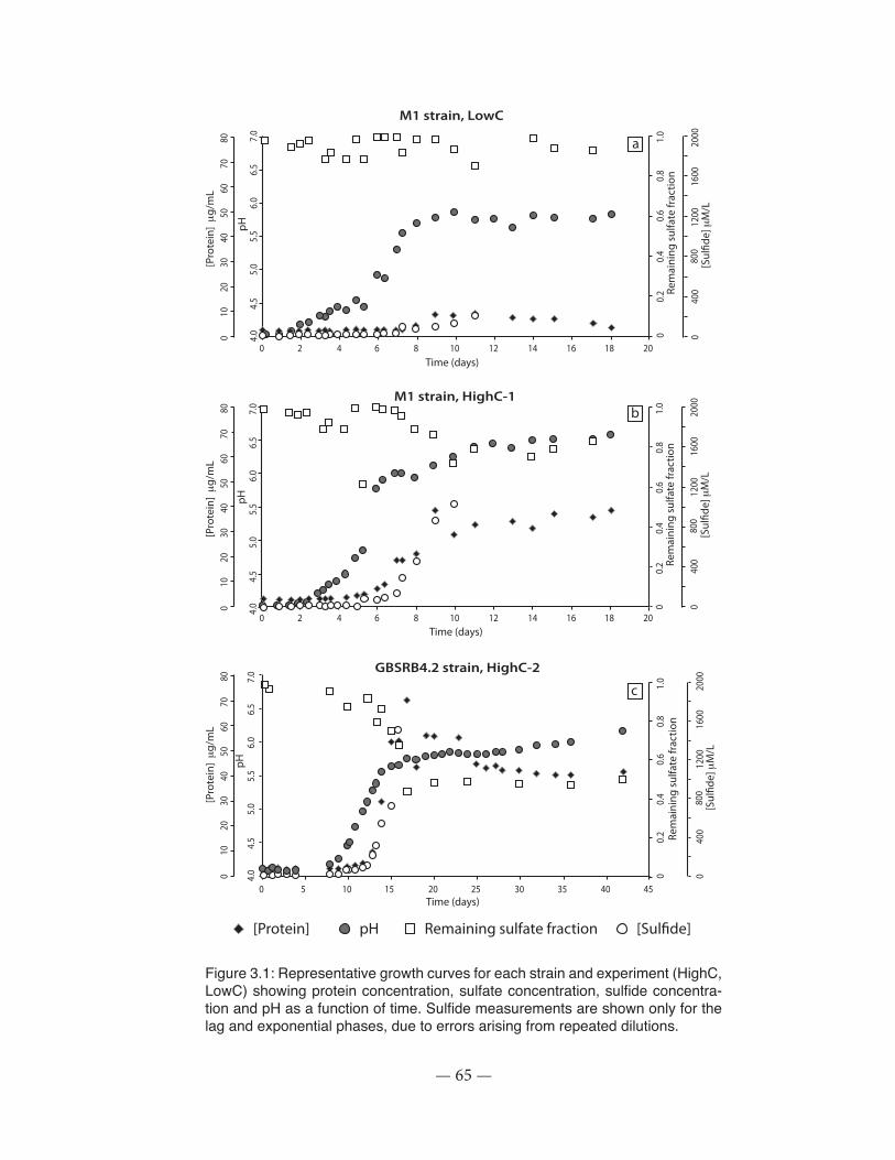
— 65 —
Figure 3.1: Representative growth curves for each strain and experiment (HighC, LowC) showing protein concentration, sulfate concentration, sulfide concentra-tion and pH as a function of time. Sulfide measurements are shown only for the lag and exponential phases, due to errors arising from repeated dilutions.
Time (days)0 2 864 141210 16 18 20
00.
60.
40.
21.
00.
8Re
mai
ning
sul
fate
frac
tion
2000
1600
1200
800
400
0[S
ul�d
e] μ
M/L
4.0
5.5
5.0
4.5
7.0
6.5
6.0
pH
010
3020
8060
5040
70[P
rote
in] μ
g/m
L
M1 strain, LowC
M1 strain, HighC-1
GBSRB4.2 strain, HighC-2
Time (days)
00.
60.
40.
21.
00.
8
4.0
5.5
5.0
4.5
6.5
6.0
0 5 201510 353025 40 45
pH
[Pro
tein
] μ
g/m
L
Rem
aini
ng s
ulfa
te fr
actio
n
[Sul
�de]
μM
/L
010
3020
8060
5040
70
2000
1600
1200
800
400
0
7.0
4.0
5.5
5.0
4.5
7.0
6.5
6.0
pH
010
3020
8060
5040
70[P
rote
in] μ
g/m
L
2000
1600
1200
800
400
0[S
ul�d
e] μ
M/L
00.
60.
40.
21.
00.
8Re
mai
ning
sul
fate
frac
tion
Time (days)0 2 864 141210 16 18 20
pH Remaining sulfate fraction[Protein] [Sul�de]
a
b
c
— 66 —
3.5.2 Stable isotopes
For both strains studied, sulfur isotopic compositions (δ34S, Δ33S) remained virtually
unchanged during the first regime, with δ34S values centered near -1‰ and Δ33S
values centered near -0.02‰ and +0.04‰ (Figure 3.2d,h). In the second regime, δ34S
values increased rapidly while Δ33S values quickly dropped suddenly (Figure 3.2d,h).
For the strain GBSRB4.2, fractionation (ε34S) during the first regime was measurable,
but low (<-0.9‰, Table 3.1). During the second regime, ε34S values were between
-10‰ and -11.5‰ (Table 3.1). For the M1 strain, fractionation was <-0.7‰ during the
first regime and between 3.7‰ and 5‰ during the second regime (Table 3.1). When
each growth regime is considered independently, fractionation was constant across
the pH range covered.
We combined data from both M1 experiments to allow for the calculation of 33λ values
using a bootstrap method: results from the GBSRB4.2 strain show that this has little
effect on the overall results (Table 3.1). Minor isotope relationships between 33S and 34S were marginally different between the two regimes, with the first regime described
by slightly higher 33λ values. However, there was no significant difference within one
standard error (Table 3.1). 33λ values measured for the M1 strain were significantly
greater than those for the GBSRB4.2 strain.

— 67 —
Figure 3.2: Protein concentration, remaining sulfate fraction f, δ34S, and Δ33S as a function of pH. The two different fractionation regimes identified in the experiments are shown.
GBSRB4.2
010
4030
2080
7060
50
3.5 4.0 5.55.04.5 7.06.56.0 3.5 4.0 5.55.04.5 7.06.56.0
3.5 4.0 5.55.04.5 7.06.56.0 3.5 4.0 5.55.04.5 7.06.56.0
3.5 4.0 5.55.04.5 7.06.56.0 3.5 4.0 5.55.04.5 7.06.56.0
3.5 4.0 5.55.04.5 7.06.56.0 3.5 4.0 5.55.04.5 7.06.56.0
0.4
0.5
0.7
0.6
1.1
1.0
0.9
0.8
-4-2
20
108
64
-0.0
8-0
.06
-0.0
4-0
.02
00.
020.
040.
06
010
4030
2080
7060
500.
40.
50.
70.
61.
11.
00.
90.
8-4
-22
010
86
4-0
.08
-0.0
6-0
.04
-0.0
20
0.02
0.04
0.06
M1[p
rote
in] μ
g/L
Frac
tio
n re
mai
nin
g s
ulfa
te, f
δ34S su
lfate
(‰)
Δ33
S sulfa
te (‰
)
pH
HighC-1HighC-2LowC
HighC-1HighC-2
Regime I Regime II Regime I Regime II
a
b
c
d
e
f
g
h
pH
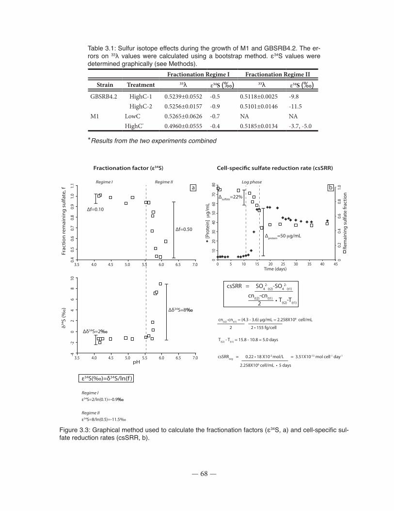
— 68 —
Table 3.1: Sulfur isotope effects during the growth of M1 and GBSRB4.2. The er-rors on 33λ values were calculated using a bootstrap method. ε34S values were determined graphically (see Methods).
Fractionation Regime I Fractionation Regime IIStrain Treatment 33λ ε34S (‰) 33λ ε34S (‰)
GBSRB4.2 HighC-1 0.5239±0.0552 -0.5 0.5118±0.0025 -9.8HighC-2 0.5256±0.0157 -0.9 0.5101±0.0146 -11.5
M1 LowC 0.5265±0.0626 -0.7 NA NAHighC* 0.4960±0.0555 -0.4 0.5185±0.0134 -3.7, -5.0
*Results from the two experiments combined
Figure 3.3: Graphical method used to calculate the fractionation factors (ε34S, a) and cell-specific sul-fate reduction rates (csSRR, b).
3.5 4.0 5.55.04.5 7.06.56.0
-4-2
20
108
64
δ34S
(‰)
3.5 4.0 5.55.04.5 7.06.56.0
0.4
0.5
0.7
0.6
1.1
1.0
0.9
0.8
Frac
tio
n re
mai
nin
g s
ulfa
te, f
Δf=0.50
Δf=0.10
Δδ34S=8‰
Δδ34S=2‰
ε34S(‰)=δ34S/ln(f )
Regime I Regime II
Regime I
ε34S=2/ln(0.1)=-0.9‰
Regime II
ε34S=8/ln(0.5)=-11.5‰
pH
Time (days)
00.
60.
40.
21.
00.
8
0 5 201510 353025 40 45
[Pro
tein
] μ
g/m
L
Rem
aini
ng s
ulfa
te fr
actio
n
010
3020
8060
5040
70
Log phase
Δprotein=50 μg/mL
Δsulfate=22%
csSRR = SO42-
(t2)-SO42-
(t1)
cn(t2)-cn(t1) = (4.3 - 3.6) μg/mL = 2.258X10⁶ cell/mL
T(t2) - T(t1) = 15.8 - 10.8 = 5.0 days
cn(t2)-cn(t1)
2 T(t2)-T(t1)•
csSRRavg = 0.22 • 18 X10-3 mol/L = 3.51X10⁻¹³ mol cell-1 day-1
2.258X10⁶ cell/mL 5 days•
2 • 155 fg/cell2
a b
Fractionation factor (ε34S) Cell-speci�c sulfate reduction rate (csSRR)

— 69 —
3.6 Discussion
A key objective of our study was to investigate the effect of pH on sulfur isotope frac-
tionation during MSR. In a closed system where the conversion of the sulfate to sul-
fide is incomplete and fractionation is constant, a plot of δ34Sreactant against the remai-
ning sulfate fraction f yields a straight line (Rayleigh distillation effect; Mariotti et al.,
1981). Our investigation of sulfur fractionation during MSR for two acidophilic strains
of sulfate-reducers shows that fractionation was not constant across the pH range of
the experiments. Two distinct regimes of fractionation were identified.
One fractionation regime (regime II) corresponds to the exponential growth and statio-
nary phases of the microbial growth cycle and is consistent with the results of previous
studies investigating sulfur isotope fractionation during microbial sulfate reduction.
This regime is characterized by rapid growth accompanied by rapid sulfate depletion
and significant sulfur isotope fractionation. Fractionation during this phase (4-12‰),
as measured using the enrichment factor ε34S, is consistent with previous measure-
ments of fractionation during MSR by incomplete oxidizers (2-19‰; Detmers et al.,
2001), as is the mass-dependent relationship between 33S and 34S, described by 33λ
(Farquhar and Wing, 2003; Johnson et al., 2005; Johnson et al., 2007; Sim et al.,
2011). There was no evidence, as expected, of mass-independent fractionation, as in-
dicated by the Δ33S values near zero. Cell-specific sulfate reduction rates were also in
the range reported for incomplete oxidation of carbon during MSR (fmoles cell-1 day-1)
[Detmers et al., 2001; Sim et al., 2011].
Where our results depart from those of previous studies is in the identification of a
distinct fractionation regime associated to the portion of the growth cycle taking place
during the lag phase, before the initiation of exponential growth and sulfate reduction.
This regime features a large increase in pH that is not accompanied by significant
microbial growth or substantial sulfur isotope fractionation. It also displays a decou-

— 70 —
pling between the initiation of a change in pH, the production of sulfide (signaling the
initiation of active sulfate reduction), and the increase in protein concentration (proxy
for cell growth). This decoupling is more apparent for the GBSRB4.2 strain, which
has a notably long lag phase, lasting up to several days (Senko et al., 2009). The
shift to the second regime appears to coincide with the beginning of the exponential
growth phase, as indicated by a rapid increase in protein concentration. This hints at a
parallel mechanism contributing to the increase of pH in the growth environment, one
not linked to the oxidation of carbon during MSR and the production of HCO3-, which
increases pH. Fractionation during this first regime is small, but measurable, with ε34S
values < 0.9‰. Most studies of sulfur isotope fractionation during sulfate reduction by
bacteria have used near-neutral pH strains that typically have relatively short growth
cycles (a few days at most): this may explain why fractionation during the lag phase
of the growth cycle has apparently not been measured previously.
A possible explanation for the change in pH prior to the initiation of microbial sulfate
reduction is internal sulfate accumulation coupled to the uptake of protons from the
solution. Significant accumulation of sulfate by sulfate-reducing bacteria has been
identified previously (Cypionka 1987; 1989). In most freshwater species, this pro-
cess is accomplished with the concurrent uptake of two or three protons via a sym-
port (Cypionka, 1987; 1989; Warthmann and Cypionka, 1990). Cells in the lag phase
may have been accumulating internal sulfate concurrently with the uptake of protons
from the growth environment, increasing pH, prior to the initiation of sulfate reduc-
tion. Fractionation during this initial regime is measurable and in the same direction
as that measured during the exponential growth phase: lighter isotopes are favored,
resulting in enrichment in 34S of the remaining sulfate. If an accumulation process is
responsible for the increase in pH prior to the initiation of sulfate reduction, our results
could represent the first successful measurement of the fractionation associated to
the first step of the sulfate reduction metabolism; the uptake of sulfate from the growth
— 71 —
environment. It should be noted that the fractionation factor measured for the first
regime is in the same order of magnitude but goes in the opposite direction of that
proposed in sulfate reduction models (e.g., Rees 1973). Further experimentation with
strains characterized by long growth cycles and lag phases are needed to test this
hypothesis.
A central objective of this study was to determine whether pH exerts an effect on frac-
tionation of sulfur during microbial sulfate reduction. We speculated that a change in
the proton gradient between the growth environment and the cytoplasm could affect
sulfur fractionation. Our results indicate that fractionation is not constant across the
pH range observed in our experiments, but it is unclear as to what mechanism is spe-
cifically responsible. If fractionation during the first phase results mostly from internal
accumulation of sulfate unaccompanied by sulfate reduction, then it is possible that
the switch to the second phase of fractionation at what appears to be a specific pH
for each strain is related to the transmembrane proton gradient (ΔpH). Studies of
internal sulfate accumulation by sulfate-reduction bacteria indicate that this parameter
exerts an effect on alkalinisation and sulfide production and drives the uptake of sul-
fate from the growth medium (Cypionka 1987; 1989), suggesting that accumulation is
enhanced at high transmembrane pH gradients, but inhibited when the environmental
pH is close to or greater than the internal pH (Warthmann and Cypionka 1990). The
switch to a different fractionation regime at a specific pH for each strain may indicate
a change in metabolic activity related to the transmembrane pH.
Our results suggest that pH exerts an effect on fractionation of sulfur isotopes insofar
as it plays a role in determining when the initiation of the bacterial sulfate reduction
process takes place: if the growth cycle of the two strains studied here is considered
in two distinct phases, then for each phase the extent of fractionation (ε34S) and the
mass-dependent relationship between 33S and 34S is constant. Our results suggest
— 72 —
that this effect of pH on fractionation is related to a change in metabolic activity and is
not gradual or progressive as pH in the growth environment is changing.
3.7 Conclusion
Our results represent the first measurement of sulfur isotope fractionation for acido-
philic sulfate reducers. We identified two regimes of fractionation that appear to be
related to a change metabolic activity. The regime corresponding to the exponential
and stationary growth phases is consistent with that identified in previous studies
and is associated with significant isotope fractionation. The regime corresponding to
the lag phase and associated to minimal sulfate reduction has to our knowledge not
been identified previously. The switch to the second fractionation regime occurred at
a specific pH for each strain and suggests that the initiation of active sulfate reduc-
tion is linked to the transmembrane pH gradient. The increase in pH during the first
regime, prior to the initiation of sulfate reduction, may be associated to internal sulfate
accumulation, with the uptake of protons concurrently with the sulfate ion leading to
an increase in pH.
3.8 Acknowledgements
We extend our thanks to John Senko (University of Akron) and D. Barrie Johnson
(Bangor University) for providing the pure cultures of acidophilic sulfate-reducing bac-
teria. We also thank John Senko and Alexandre Poulain (University of Ottawa) for
helpful discussions, and Marc-André Cyr, Kizil Reder, André Pelletier, Thi Hao Bui and
Grant Cox for lab assistance. Funding for this study was provided through NSERC
Discovery Grants (DF and BW) and an NSERC Post-Graduate Scholarship (MLC).

— 73 —
Chapter 4 : Sulfur isotopes reveal that peak of Deccan vol-canism post-dates the Cretaceous-Paleogene mass extinc-tion
4.1 Contributions
The samples used in this study were collected by François Therrien and colleagues
from the Royal Tyrell Museum of Paleontology (Drumheller, Alberta) for the purposes
of investigating the stable carbon isotope and pollen records of the two KPg boundary
sections featured in this study (Therrien et al., 2007). The candidate prepared and
analysed the samples for sulfur concentration and sulfur stable isotope composition,
in collaboration with Teruyuki Maruoka at the University of Tsukuba, Tsukuba, Japan
(Graduate School of Life and Environmental Sciences), during a research internship
under the auspices of the NSERC Japan Summer Program (2010). The data analysis
and interpretation, and the preparation of the manuscript and figures were a joint effort
between the candidate and Boswell Wing (Dept. Earth and Planetary Sciences, Mc-
Gill University). François Therrien, Teruyuki Maruoka and Danielle Fortin commented
on an earlier version of the manuscript.
Cousineau, M.L., Therrien, F., Maruoka, T., Fortin, D., and Wing, B.A. In preparation
— 74 —
4.2 Abstract
The mass extinction at the Cretaceous-Paleogene (KPg) boundary decimated marine
and terrestrial species around the globe. Two major geologic events, the Chicxulub
bolide impact and the eruption of the Deccan continental flood basalts, coincide with
the KPg boundary and have been identified as possible triggers for the extinction, but
their relative timing remains unresolved. From measurements of sulfur abundance
and isotope composition at an exceptionally well-preserved terrestrial KPg boundary
section in Alberta, Canada, we demonstrate that the peak of Deccan volcanism post-
dates the Chicxulub impact and the associated abrupt KPg mass extinction. The late
occurrence of Deccan volcanism precludes a direct causal relationship with the mass
extinction, but sheds light on underlying causes for the delayed recovery of ecosys-
tems in the early Paleogene.
4.3 Main Text
The Cretaceous-Paleogene (KPg) boundary marks one of the most significant biotic
turnovers in Earth history (1, 2), leaving an evolutionary imprint that can still be seen
in the modern biota (3). The KPg mass extinction selectively reshaped marine and
terrestrial ecosystems (4-7) and ultimately led to the demise of dinosaurs and sub-
sequent radiation of mammals (2, 5, 8). Despite more than thirty years of research,
the hypothesis of an extraterrestrial cause for the KPg extinctions (9), with dust from
a bolide impact shading Earth’s surface and leading to the catastrophic collapse of
global food webs, still causes controversy (10-14). The primary competing hypothesis
to an impact-driven mass extinction links the emplacement of the Deccan Traps –
continental flood basalts that cover a surface area of ≈500 000 km2 in western India
(15) – to the KPg biotic crisis, either as a sole actor or against a backdrop of falling
sea levels and fluctuating global temperatures (10-14, 16). Although impact- and vol-

— 75 —
canism-driven extinction scenarios predict different extinction patterns (5, 17, 18), the
establishment of causal relationships relies fundamentally on the relative timing of
extinction triggers across the KPg boundary. Radiometric and magnetostratigraphic
age measurements show that the largest Deccan eruptions and the Chicxulub impact
were roughly contemporaneous across the KPg boundary (16, 19), but are too uncer-
tain to determine the relative timing of these events.
A common feature of both proposed triggers is the associated atmospheric release
of massive amounts of sulfur (20, 21). In an oxidizing atmosphere, enhanced atmos-
pheric S input is expected to increase the atmospheric burden of sulfate aerosols,
disrupting Earth’s radiative balance (22). The climatic effects of this S, along with
dust, halogens, and CO2, are a critical component of extinction scenarios accompa-
nying the Chicxulub impact and Deccan eruptions (10-14). Injection of sulfur, dust and
ash particles into the stratosphere, where global dispersion can occur rapidly, has
been directly observed for volcanic events many orders of magnitude less energetic
than the Chicxulub impact (22). For example, global climatic change followed the
1991 eruption of Mount Pinatubo (23), which explosively introduced 9 Teragrams of
S (Tg S) (24) on top of a natural background volcanic S flux of 9 – 46 Tg S per year
(25). Estimates of atmospheric S injections from the Chicxulub impact dwarf these
numbers: ≈0.4 to 5.6 × 10⁵ Tg S may have been released almost instantaneously into
the atmosphere (21). In comparison, the S released over the full eruptive history of the
Deccan Traps could have ranged from ≈1.7 to 3.5 × 10⁶ Tg S (20, 26), with atmosphe-
ric S loadings from the largest single eruptive events potentially comparable to that
from the Chicxulub impact (26).
Sulfur released by the Chicxulub impact would have primarily been derived from late
Maastrichtian seawater and the ≈3-km-thick sequence of Cretaceous evaporite- and
carbonate-bearing target rocks present at the impact site (27), whereas sulfur released
— 76 —
by Deccan volcanism would have an igneous origin. Maastrichtian seawater, Upper
Cretaceous evaporites, and Chicxulub target evaporites have δ34S values centered
around ≈18‰ (28-30) while sulfate aerosols collected at active basaltic vents are cha-
racterized by much lower δ34S values [≈8‰ (31)]. Consequently, in KPg stratigraphic
sections characterized by low sulfur content, such as those deposited in terrestrial
settings, S isotope profiles should reflect the relative contributions of impact- versus
volcanism-derived S (32).
The Knudsen’s Coulee Section (KCS) and Knudsen’s Farm Section (KFS), located
near the town of Drumheller, Alberta, Canada (Fig. 4.S1), are among the most com-
plete and best-preserved terrestrial KPg sections in North America’s Western Inte-
rior. These sections features lithological, paleontological, and geochemical markers
indicative of the terrestrial KPg boundary including, at KCS, a three-part boundary
claystone layer representing the initial ballistic melt ejecta, an early-formed ‘fireball’
layer of condensed vapor from the impactor and target rocks, and a later-formed layer
of fine particles rich in Ir and sulfate aerosols (33). In order to constrain the relative
timing of the Chicxulub impact and Deccan volcanism, we measured whole-rock S
content and isotopic composition (δ34S) at an ultrahigh stratigraphic resolution (2 cm
or less) at these sections. We focus our discussion on the KCS because it is excep-
tionally well preserved (33).
Sulfur contents and δ34S values show similar behavior at the KCS (Fig. 4.1A, 4.1B).
Below the KPg boundary claystone, S contents are extremely low, generally less than
0.2 wt%, while δ34S values vary mildly (±2‰) around a mean value of ≈6.5‰. These
features provide a favorable backdrop for monitoring 34S-rich S addition to the sulfur-
poor KCS sedimentary system. Within the three-part boundary claystone, S contents
stay below 0.1 wt% in the first two subunits (hackly and satiny layers) but increase
dramatically to ≈0.7 wt% in the uppermost subunit (laminated shale). Bulk δ34S values
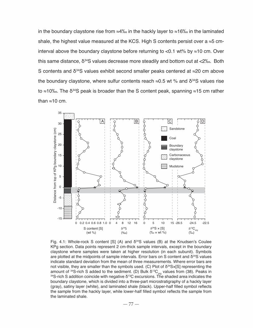
— 77 —
in the boundary claystone rise from ≈4‰ in the hackly layer to ≈16‰ in the laminated
shale, the highest value measured at the KCS. High S contents persist over a ≈5 cm-
interval above the boundary claystone before returning to <0.1 wt% by ≈10 cm. Over
this same distance, δ34S values decrease more steadily and bottom out at <2‰. Both
S contents and δ34S values exhibit second smaller peaks centered at ≈20 cm above
the boundary claystone, where sulfur contents reach ≈0.5 wt % and δ34S values rise
to ≈10‰. The δ34S peak is broader than the S content peak, spanning ≈15 cm rather
than ≈10 cm.
-15
-10
5
0
-5
10
15
20
25
30
35
0 4 128 16 0 5 10 150 0.2 0.4 0.6 0.8 1.0
S content [S] (wt %)
δ34S(‰)
δ34S × [S] (‰ × wt %)
-26.5 -24.5 -22.5
δ13Corg(‰)
Dis
tanc
e fro
m to
p of
KPg
bou
ndar
y cl
ayst
one
(cm
) Sandstone
Mudstone
Coal
Carbonaceousclaystone
Boundaryclaystone
A B C D
Cousineau et al. -- Figure 1
Fig. 4.1: Whole-rock S content [S] (A) and δ34S values (B) at the Knudsen’s Coulee KPg section. Data points represent 2 cm-thick sample intervals, except in the boundary claystone where samples were taken at higher resolution (in each subunit). Symbols are plotted at the midpoints of sample intervals. Error bars on S content and δ34S values indicate standard deviation from the mean of three measurements. Where error bars are not visible, they are smaller than the symbols used. (C) Plot of δ34S×[S] representing the amount of 34S-rich S added to the sediment. (D) Bulk δ13Corg values from (38). Peaks in 34S-rich S addition coincide with negative δ13C excursions. The shaded area indicates the boundary claystone, which is divided into a three-part microstratigraphy of a hackly layer (gray), satiny layer (white), and laminated shale (black). Upper-half filled symbol reflects the sample from the hackly layer, while lower-half filled symbol reflects the sample from the laminated shale.

— 78 —
The close correspondence between increases in S contents ([S]) and δ34S values
throughout the KCS section suggests that addition of 34S-rich S occurred across the
KPg boundary. This hypothesis is corroborated by variations in δ34S×[S], a quantity
that provides an estimate of the amount of 34S-rich S in the system and emphasizes
changes in 34S-rich S relative to background conditions (Fig. 4.1C). The δ34S×[S]
profile shows little deviation from background values except for two distinct peaks: an
asymmetrical peak, starting in the upper boundary claystone and irregularly declining
over the next 10 cm, and a second, more moderate and symmetrical peak situated 17-
23 cm above the boundary claystone. These peaks indicate that addition of 34S-rich
sulfur took place during two discrete time intervals in the early Paleogene.
This 34S-rich sulfur was added to a S-poor and low-δ34S background population at
the KCS, defined by a cluster of ≈10 points on a cross-plot of δ34S values and [S]
(Fig. 4.2). With increasing S content, one array of measurements extends from this
background population to a plateau around δ34S values approaching ≈8‰ (Fig. 4.2).
A second array of measurements rises more rapidly, and levels out around a much
higher δ34S value approaching ≈18‰ (Fig. 4.2). The hyperbolic forms of these arrays
are consistent with addition of sulfur from two distinct 34S-rich S sources (33). The
δ34S value for the end-member of the lower array of samples is similar to sulfate
aerosols from volcanogenic S oxidized at active sites of basaltic degassing (Fig. 4.2;
(31)), whereas that of the end-member of the upper array of samples is comparable
to Chicxulub target rocks, Upper Cretaceous evaporites and Maastrichtian seawater
(Fig. 4.2; (28-30)). The lack of volcanic detritus in the 34S-rich S parts of the KCS sug-
gests a distal source for the volcanic sulfur identified here. Accordingly, we propose
that the KCS section contains 34S-rich S derived from Deccan volcanism and the
Chicxulub impact. Our high-resolution sampling at the KCS has permitted, for the first
time, recognition of the S isotope signatures of both terminal Cretaceous events at a
single location.
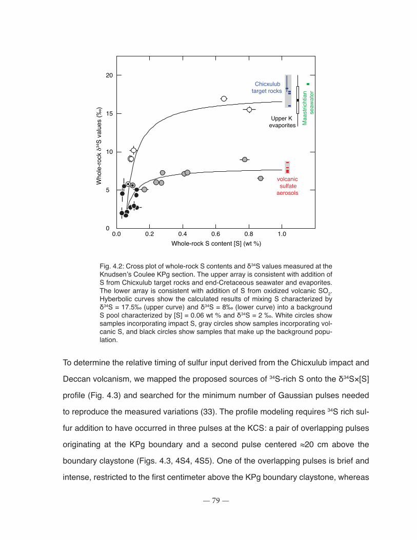
— 79 —
Fig. 4.2: Cross plot of whole-rock S contents and δ34S values measured at the Knudsen’s Coulee KPg section. The upper array is consistent with addition of S from Chicxulub target rocks and end-Cretaceous seawater and evaporites. The lower array is consistent with addition of S from oxidized volcanic SO2. Hyberbolic curves show the calculated results of mixing S characterized by δ34S = 17.5‰ (upper curve) and δ34S = 8‰ (lower curve) into a background S pool characterized by [S] = 0.06 wt % and δ34S = 2 ‰. White circles show samples incorporating impact S, gray circles show samples incorporating vol-canic S, and black circles show samples that make up the background popu-lation.
To determine the relative timing of sulfur input derived from the Chicxulub impact and
Deccan volcanism, we mapped the proposed sources of 34S-rich S onto the δ34S×[S]
profile (Fig. 4.3) and searched for the minimum number of Gaussian pulses needed
to reproduce the measured variations (33). The profile modeling requires 34S rich sul-
fur addition to have occurred in three pulses at the KCS: a pair of overlapping pulses
originating at the KPg boundary and a second pulse centered ≈20 cm above the
boundary claystone (Figs. 4.3, 4S4, 4S5). One of the overlapping pulses is brief and
intense, restricted to the first centimeter above the KPg boundary claystone, whereas
0
5
10
15
20
0.0 0.2 0.4 0.6 0.8 1.0
volcanic sulfateaerosols
Chicxulub target rocks
Upper K evaporites M
aast
richt
ian
seaw
ater
Whole-rock S content [S] (wt %)
Who
le-ro
ck δ
34S
valu
es (‰
)
Cousineau et al. -- Figure 2

— 80 —
the other is wider and more moderate, spanning a 10-cm interval above the boundary
claystone. Based on the inferred 34S-rich S source of each sample, we conclude that
the spike at the KPg boundary is derived from the injection of impact-derived sulfate
aerosols while the two broad pulses record addition of Deccan volcanic sulfate. These
results reveal that the Chicxulub bolide impact coincided with the beginning of a Dec-
can volcanic eruptive phase at the KPg boundary (Fig. 4.3).
Recent high-resolution measurements of 187Os/188Os values from marine sediments
are seemingly in conflict with this proposal. They show an initial decline at the start
of magnetic polarity chron C29r (≈300 kyrs before the KPg boundary), followed by
a brief plateau of unchanging values, and then a sharp decrease coinciding with Ir
maxima (34, 35). This record is interpreted as an initial input of Deccan volcanic Os
preceding the impact-induced isotopic signal at the KPg boundary. However, mass
balance calculations suggest that the initial decline in 187Os/188Os values is too large
to be strictly the result of an increased input of non-radiogenic Os from the Deccan
basalts; removal of a source of radiogenic Os is also necessary (34, 35). Low-volume,
early-erupted Deccan flows, if they covered Archean crust, would have had the requi-
red effect (35). The pre-KPg boundary 187Os/188Os record may only signal the initiation
of main-phase Deccan volcanism (34), while the S isotope record instead reflects
the intensity, duration, and frequency of the full Deccan eruptive history. In addition,
seismic reflection, magnetic, and gravity data reveal a substantial pre-Deccan (Cam-
panian-Maastrichtian) volcanostratigraphic province off the Western shore of India,
with a minimum estimated volume ≈20-25% of the Deccan continental flood basalts
(36). The submarine nature of this pre-Deccan eruption would lead to a direct transfer
of volcanic Os to the oceanic environment, suggesting that it could have caused the
marine 187Os/188Os drop prior to the KPg boundary. Any S emissions accompanying a
submarine volcanic eruption, however, would be unlikely to leave an S isotope signal
in terrestrial sediments. Given these viable explanations for the apparent discrepancy
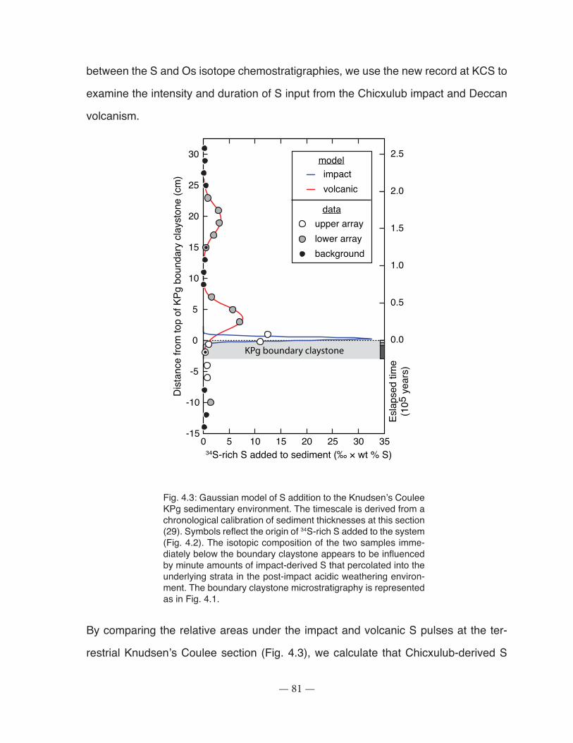
— 81 —
between the S and Os isotope chemostratigraphies, we use the new record at KCS to
examine the intensity and duration of S input from the Chicxulub impact and Deccan
volcanism.
-15
-10
-5
0
5
10
15
20
25
30
KPg boundary claystone
34S-rich S added to sediment (‰ × wt % S)
Dis
tanc
e fro
m to
p of
KPg
bou
ndar
y cl
ayst
one
(cm
)
0 5 10 15 20 25 30 35
volcanicimpact
0.5
1.0
1.5
2.0
2.5
Esla
psed
tim
e(1
05 y
ears
)
0.0
backgroundlower arrayupper array
data
model
Cousineau et al. -- Figure 3
Fig. 4.3: Gaussian model of S addition to the Knudsen’s Coulee KPg sedimentary environment. The timescale is derived from a chronological calibration of sediment thicknesses at this section (29). Symbols reflect the origin of 34S-rich S added to the system (Fig. 4.2). The isotopic composition of the two samples imme-diately below the boundary claystone appears to be influenced by minute amounts of impact-derived S that percolated into the underlying strata in the post-impact acidic weathering environ-ment. The boundary claystone microstratigraphy is represented as in Fig. 4.1.
By comparing the relative areas under the impact and volcanic S pulses at the ter-
restrial Knudsen’s Coulee section (Fig. 4.3), we calculate that Chicxulub-derived S
— 82 —
accounts for ≈16% of the total amount of sulfur added to the KCS sedimentary envi-
ronment (33). The volcanic pulse at the boundary accounts for ≈54% of the added S,
while the second volcanic pulse accounts for ≈30% (33). This yields a ratio of ≈5.5:1
for sulfur derived from Deccan volcanism relative to the Chicxulub impact, in line with
independent published estimates, which range from 3:1 to 88:1 (see above). The
second volcanic pulse, although recorded over a similar length interval to the first
eruptive pulse, represents only about half of its intensity in terms of S addition to the
KCS sedimentary environment. This is consistent with estimates of S fluxes for the
two later phases of Deccan volcanism (26).
The duration of the volcanic pulses can be estimated based on the chronological cali-
bration of sediment thicknesses at KCS (33). Any estimate of the duration of the im-
pact-derived sulfur pulse would be overestimated, due to the integrated nature of our
sampling method. The first pulse of S input from Deccan volcanism, which began at
the KPg boundary, ended ≈90 kyrs after the impact. A second, more moderate, pulse
of volcanic S addition began approximately 30 kyrs later and lasted for ≈90 kyrs. Aside
from a minor, geographically-restricted early phase of volcanism occurring ≈2-3 mil-
lion years prior to the KPg boundary (26), current interpretations call on two brief,
intense, and closely spaced phases of Deccan eruptions lasting 200-300 kyrs (19,
26), consistent with our environmental scenario.
Where our environmental scenario departs significantly from previous interpretations
of the KPg transition is in the relative timing of the two proposed extinction triggers.
Some stratigraphic examinations of the relationship between impact and volcanism
suggest that the impact emplacement of the Ir-rich KPg claystone layer took place
at the end of a major volcanic phase (16, 34, 37). In a recent paleomagnetic and
geochronological reconstruction of Deccan eruptions, the major volcanic phase was
positioned as starting before the KPg boundary and ending precisely at the boundary,

— 83 —
followed by a less intense phase of eruptions (19). However, an internally-consistent
reconstruction of absolute ages across the KPg boundary shows that many of the
stratigraphically-controlled main phase Deccan flows could have erupted after the
impact defining the KPg boundary (Fig. 4.S7). The KCS S isotope profile, in fact,
demonstrates that this is the case. The Chicxulub impact coincided with the beginning
of the main Deccan volcanic eruptive phase at the KPg boundary, this main phase
lasted for ≈90 kyrs, and the secondary eruptive phase started ≈30 kyrs after the main
phase ended, lasting for another ≈90 kyrs (Fig. 4.3).
Fig. 4.4 Chronology of environmental and biological events across the KPg boundary in the Northern Hemisphere. Records prior to the KPg boundary are not chronologically calibrated but are included for reference. (A) Ecological recovery in terrestrial floras as monitored by δ13Corg values and dominant flo-ral assemblages at Knudsen’s Coulee KPg section (29). (B) Relative timing of KPg boundary, Chicxu-lub impact S input (shown in blue, unscaled), and the two major phases of Deccan volcanism (shown in red). Recovery dynamics of terrestrial faunas from the Western Interior are superimposed (39). (C) Early ecological recovery in the pelagic marine environment as monitored by surface-to-deep δ13C gradients and community structure from ODP hole 1209, Shatsky Rise, North Pacific (43).
-23
-24
-25
-26
Bulk
org
anic
δ13
C (‰
)Su
rface
-to-d
eep
δ13C
diff
eren
ce (‰
)
KPg 100 200 300 400Elapsed time since KPg Boundary (kyrs)
B
A
C
Angiosperm &gymnosperm
Angiosperm & fern
Fern
Angiosperm &gymnosperm
Cretaceous dinosaur-dominated fauna
Earliest Paleogene low-diversity, small body-sized mammal fauna
Earliest proposed recoveryof pre-KPg mammal species richness
Cretaceoushigh-diversityplanktonicassemblage
Earliest Paleogene low-diversity,early recovery planktonic community
0.0
1.0
2.0
Full replacement of early recovery planktonic community
chronologicallyuncalibrated
Rel
ativ
e in
tens
ity o
f D
ecca
n er
uptio
ns (%
)
100
50
Cousineau et al. -- Figure 4
0
— 84 —
Our new high-resolution environmental chronology indicates that the Chicxulub im-
pact was the primary trigger for the KPg mass extinction, and argues against a causal
relationship between Deccan volcanism and the extinctions. However, the massive
amounts of sulfur released by the Deccan eruptions must have had deleterious ecolo-
gical consequences (12, 20), raising the possibility that Deccan eruptions could have
led to the delayed recovery of Paleogene ecosystems. Patterns of 34S-rich S addition
and δ13C values in terrestrial organic matter show a clear inverse correlation throu-
ghout the KCS and KFS (Figs. 4.1, 4.S3). Minimum δ13Corg values are reached during
the peak of the major Deccan eruptive phase while pre-boundary δ13Corg values and
floral compositions return right after the first volcanic phase ended, ≈100 kyrs into the
Paleogene ((38); Fig. 4.4A, 4.4B). In the Western Interior, depauperate and small-
sized terrestrial vertebrate faunas characteristic of the earliest Paleogene began their
recovery between ≈200 and 400 kyrs after the KPg boundary ((39, 40); Fig. 4.4B), in
general coincidence with the end of the secondary Deccan eruptive phase. Surface-
to-deep δ13C profiles through deep sea sediments show that marine ecosystems ex-
perienced longer-lasting perturbations ((41); Fig. 4.4C), perhaps initially resulting from
volcanically-induced metal poisoning (18) or ocean acidification (42). Early commu-
nities of bloom and disaster taxa dominated pelagic ecosystems for ≈450 kyrs in the
North Pacific ((43); Fig. 4.4C), suggesting that the initiation of marine ecosystem reco-
very was delayed until after the complete cessation of Deccan eruptions. Although the
Chicxulub impact may have triggered the KPg boundary mass extinction, the major
eruptive phases of the Deccan Traps appear to have paced the tempo of marine and
terrestrial ecosystem recovery into the brave new Paleogene world.
— 85 —
4.4 References and Notes
1. J. Alroy, Dynamics of origination and extinction in the marine fossil record. Pro-
ceedings of the National Academy of Sciences of the United States of America 105,
11536-11542 (2008).
2. R. Meredith et al., Impacts of the Cretaceous terrestrial revolution and KPg extinc-
tion on mammal diversification. Science 334, 521-524 (2011).
3. A. Krug, D. Jablonski, J. Valentine, Signature of the End-Cretaceous mass extinc-
tion in the Modern Biota. Science 323, 767-771 (2009).
4. D. J. Nichols, K. R. Johnson, Plants and the K-T Boundary (Cambridge University
Press, Cambridge, 2008), p. 280.
5. J. D. Archibald, Extinction and radiation: How the fall of dinosaurs led to the rise of
mammals (The Johns Hopkins University Press, Baltimore, 2011), p. 108.
6. S. D’Hondt, Consequences of the cretaceous/paleogene mass extinction for ma-
rine ecosystems. Annual Review of Ecology Evolution and Systematics 36, 295-317
(2005).
7. P. Sheehan, D. Fastovsky, Major extinctions of land-dwelling vertebrates at the Cre-
taceous-Tertiary Boundary, Eastern Montana. Geology 20, 556-560 (1992).
8. F. Smith et al., The evolution of maximum body size of terrestrial mammals. Science
330, 1216-1219 (2010).
9. L. W. Alvarez, W. Alvarez, F. Asaro, H. V. Michel, Extraterrestrial cause for the
Cretaceous-Tertiary extinction - Experimental results and theoretical interpretation.
Science 208, 1095-1108 (1980).
10. P. Schulte et al., The Chicxulub asteroid impact and mass extinction at the Creta-
— 86 —
ceous-Paleogene Boundary. Science 327, 1214-1218 (2010).
11. J. Archibald et al., Cretaceous Extinctions: Multiple Causes. Science 328, 973
(2010).
12. V. Courtillot, F. Fluteau, Cretaceous extinctions: The volcanic hypothesis. Science
328, 973-974 (2010).
13. G. Keller et al., Cretaceous extinctions: Evidence overlooked. Science 328, 974-
975 (2010).
14. P. Schulte et al., Response - Cretaceous extinctions. Science 328, 975-976 (2010).
15. A. Jay, M. Widdowson, Stratigraphy, structure and volcanology of the SE Deccan
continental flood basalt province: implications for eruptive extent and volumes. Jour-
nal of the Geological Society 165, 177-188 (2008).
16. G. Keller, T. Adatte, S. Gardin, A. Bartolini, S. Bajpai, Main Deccan volcanism
phase ends near the K-T boundary: Evidence from the Krishna-Godavari Basin, SE
India. Earth and Planetary Science Letters 268, 293-311 (2008).
17. V. Vajda, J. Raine, C. Hollis, Indication of global deforestation at the Cretaceous-
Tertiary boundary by New Zealand fern spike. Science 294, 1700-1702 (2001).
18. S. Jiang, T. Bralower, M. Patzkowsky, L. Kump, J. Schueth, Geographic controls
on nannoplankton extinction across the Cretaceous/Palaeogene boundary. Nature
Geoscience 3, 280-285 (2010).
19. A. Chenet, X. Quidelleur, F. Fluteau, V. Courtillot, S. Bajpai, 40K-40Ar dating of the
Main Deccan large igneous province: Further evidence of KTB age and short dura-
tion. Earth and Planetary Science Letters 263, 1-15 (2007).
20. S. Self, S. Blake, K. Sharma, M. Widdowson, S. Sephton, Sulfur and chlorine in
— 87 —
Late Cretaceous Deccan magmas and eruptive gas release. Science 319, 1654-1657
(2008).
21. E. Pierazzo, D. Kring, H. Melosh, Hydrocode simulation of the Chicxulub impact
event and the production of climatically active gases. Journal of Geophysical Re-
search-Planets 103, 28607-28625 (1998).
22. O. Toon, K. Zahnle, D. Morrison, R. Turco, C. Covey, Environmental perturbations
caused by the impacts of asteroids and comets. Reviews of Geophysics 35, 41-78
(1997).
23. P. Minnis et al., Radiative climate forcing by the Mount-Pinatubo eruption. Science
259, 1411-1415 (1993).
24. S. Guo, G. Bluth, W. Rose, I. Watson, A. Prata, Re-evaluation of SO2 release of
the 15 June 1991 Pinatubo eruption using ultraviolet and infrared satellite sensors.
Geochemistry Geophysics Geosystems 5, 1525-2027 (2004).
25. C. Oppenheimer, B. Scaillet, R. Martin, Sulfur degassing from volcanoes: Source
conditions, surveillance, plume chemistry and Earth system impacts. Reviews in Mi-
neralogy and Geochemistry 73, 363-421 (2011).
26. A. Chenet et al., Determination of rapid Deccan eruptions across the Cretaceous-
Tertiary boundary using paleomagnetic secular variation: 2. Constraints from analysis
of eight new sections and synthesis for a 3500-m-thick composite section. Journal of
Geophysical Research-Solid Earth 114, 38 pp., B06103, doi:10.1029/2008JB005644
(2009).
27. H. Sigurdsson et al., Geochemical constraints on source region of Cretaceous
Tertiary impact glasses. Nature 353, 839-842 (1991).
28. A. Paytan, M. Kastner, D. Campbell, M. H. Thiemens, Seawater sulfur isotope
— 88 —
fluctuations in the Cretaceous. Science 304, 1663-1665 (2004).
29. C. Koeberl, Chicxulub crater, Yucatan - Tektites, impact glasses, and the geoche-
mistry of target rocks and breccias. Geology 21, 211-214 (1993).
30. G. E. Claypool, W. T. Holser, I. R. Kaplan, H. Sakai, I. Zak, The age curves of
sulfur and oxygen isotopes in marine sulfate and their mutual interpretation. Chemical
Geology 28, 199-260 (1980).
31. T. Mather et al., Oxygen and sulfur isotopic composition of volcanic sulfate aerosol
at the point of emission. Journal of Geophysical Research-Atmospheres 111, 9 pp.,
D18205, doi:10.1029/2005JD006584 (2006).
32. E. C. Perry, D. J. Winter, B. Sagar, B. Wu, The Chicxulub structure: Surface mani-
festation and possible sulfur isotope signature, Lunar and Planetary Institute Science
Conference Abstracts, 23, p. 1057 (1992).
33. Supplementary Online Material.
34. N. Robinson, G. Ravizza, R. Coccioni, B. Peucker-Ehrenbrink, R. Norris, A high-
resolution marine 187Os/188Os record for the late Maastrichtian: Distinguishing the che-
mical fingerprints of Deccan volcanism and the KP impact event. Earth and Planetary
Science Letters 281, 159-168 (2009).
35. G. Ravizza, B. Peucker-Ehrenbrink, Chemostratigraphic evidence of Deccan vol-
canism from the marine osmium isotope record. Science 302, 1392-1395 (2003).
36. G. Calves et al., Seismic volcanostratigraphy of the western Indian rifted margin:
The pre-Deccan igneous province. Journal of Geophysical Research-Solid Earth 116,
28 pp., B01101, doi:10.1029/2010JB000862 (2011).
37. V. Courtillot et al., Cosmic markers, 40Ar/39Ar dating and paleomagnetism of the KT
— 89 —
sections in the Anjar Area of the Deccan large igneous province. Earth and Planetary
Science Letters 182, 137-156 (2000).
38. F. Therrien, D. Eberth, D. Braman, D. Zelenitsky, High-resolution organic carbon
isotope record across the Cretaceous-Tertiary boundary in south-central Alberta: Im-
plications for the post-impact recovery rate of terrestrial ecosystems and use of δ13C
as a boundary marker. Canadian Journal of Earth Sciences 44, 529-542 (2007).
39. W. A. Clemens, Evolution of the mammalian fauna across the Cretaceous-Ter-
tiary boundary in northeastern Montana and other areas of the Western Interior. 361,
217-245 (2002).
40. J. A. Lillegraven, J. J. Eberle, Vertebrate faunal changes through Lancian and
Puercan time in southern Wyoming. Journal of Paleontology 73, 691-710 (1999).
41. S. D’Hondt, P. Donaghay, J. Zachos, D. Luttenberg, M. Lindinger, Organic carbon
fluxes and ecological recovery from the Cretaceous-Tertiary mass extinction. Science
282, 276-279 (1998).
42. L. Alegret, E. Thomas, K. Lohmann, End-Cretaceous marine mass extinction not
caused by productivity collapse. Proceedings of the National Academy of Sciences of
the United States of America 109, 728-732 (2012).
43. P. Hull, R. Norris, T. Bralower, J. Schueth, A role for chance in marine recovery
from the end-Cretaceous extinction. Nature Geoscience 4, 856-860 (2011).

— 90 —
4.5 Acknowledgements
Data measured for this study are available in the Supporting Online Materials. This
study was made possible by a fellowship from the Japan Society for the Promotion of
Science to MLC, and by the National Science and Engineering Research Council of
Canada, through fellowships to MLC and FT and Discovery grants to DF and BAW.
We thank Kent and Marian Knudsen for allowing free access to their property, Dennis
Braman for assistance in sampling, Craig Scott for fruitful discussions, and Pincelli
Hull for providing δ13C data from ODP Hole 1209.
— 91 —
4.6 Supplementary Materials:
4.6.1 Detailed geology
The Knudsen’s Coulee (KCS, 51°53’15’’N; 113°01’46’’W) and Knudsen’s Farm (KFS,
51°54’32’’N; 113°02’59’’W) Cretaceous-Paleogene (KPg) boundary sections are loca-
ted 2.5 km apart on the Knudsen’s T. rex Ranch, in the valley of the Red Deer River,
north of the town of Drumheller, Alberta, Canada (Fig. 4.S1). Both sections preserve
excellent exposures of the Scollard Formation (Edmonton Group), which consists
mostly in drab-coloured mudstones and sandstones deposited in an alluvial plain de-
veloped in response to the Cordilleran Orogeny (Richardson et al., 1988; Catuneanu
and Sweet, 1999). The age of the Scollard Formation has been constrained to the late
Maastrichtian through the early Paleocene using radiometric, biostratigraphic and ma-
gnetostratigraphic methods (Srivasta, 1970; Lerbekmo and Coulter, 1985; Lerbekmo
and Braman, 2002). The lower portion of the Scollard Formation is equivalent in age
to the Hell Creek Formation of Montana and South Dakota, the Lance Formation of
Wyoming, and the Frenchman Formation of Saskatchewan. Typical Late Cretaceous
vertebrate fossil remains, including those of Tyrannosaurus and Triceratops, can be
found in strata below the KPg boundary at both localities. Palynofloral successions
across the KPg boundary are also comparable at both sections (Lerbekmo et al.,
1987; Sweet and Braman, 1992).

— 92 —
Fig. 4.S1: Location of the Knudsen’s T. rex Ranch near Dru-mheller, Alberta, Canada. The Knudsen’s Coulee and Knud-sen’s Farm KPg sections are 2.5 km apart on this property. The KPg sections on the Knudsen’s property represent the farthest known extent the hackly ejecta layer. Figure modified from Sweet and Braman (2001).
4.6.1.1 Knudsen’s Coulee Section
At the Knudsen’s Coulee Section, the KPg boundary is exposed continuously over
50 m and discontinuously over 150 m of the Scollard Formation. The lowermost stra-
tum of the section consists in gray mudstone, which contains root traces and is inter-
preted to represent the Bg horizon of a hydromorphic paleosol (Fig. 4.1). It is overlain
4300 km
Chicxulub Structure
Knudsen’sT. rex Ranch
CANADAU.S.A.
Sask
atch
ewan
Albe
rtaNorth
Montana
Wyoming Colorado
Preserved terrestrial sediments contiguous to the KPg boundary
N
0 500 km
Dakota
Cousineau et al. -- Figure S1

— 93 —
by 6 cm of carbonaceous claystone forming the base of the Nevis coal (#13; Gibson,
1977). The 3.0-cm thick boundary claystone is overlain by 32 cm of Nevis coal, the top
of which is truncated by a 48 cm-thick sandstone body. At this locality, the composite
claystone layer recognized as the KPg boundary claystone (Hildebrand and Boynton,
1988b) can be subdivided into three subunits (Fig. 4.S2) [Sweet et al., 1999]. The
lowermost unit, the “hackly claystone” layer, is a 2.2-cm thick layer of light brownish
grey claystone that represents weathered micro-spherules and micro-tecktites (Hilde-
brand, 1993). The middle 0.4-cm thick layer of “satiny claystone” is pinkish brown with
a satiny luster. It contains “graupen” pellets, is gradational in texture with the over-
lying laminated shale and contains abundant shocked quartz (Lerbekmo et al., 1999).
The topmost dark-brown “laminated shale” layer is 0.4-cm thick and contains 10-20
claystone laminae separated primarily by organic debris. It includes abundant shoc-
ked quartz and is easily distinguished from the hackly and satiny layers by its fissile
nature. The hackly claystone, satiny claystone, and laminated shale microstratigra-
phy of the boundary claystone at the KCS are thought to represent, respectively, the
ejecta layer, the fireball layer, and the layer of sulfur aerosols and condensate from the
vaporized target and impacting body (Sweet et al, 1999). Iridium abundance profiles
show maximum abundance within the boundary claystone in the satiny claystone and
laminated shale layers (9.62 ± 0.06 and 9.27 ± 0.11 ppb, respectively; Lerbekmo et
al., 1996). In a high-resolution study of carbon isotopes at the KCS and KFS, Therrien
et al. (2007) found a 1.8 to 2.3‰ excursion starting in the satiny claystone layer. They
used the carbon isotope and carbon content profiles, combined with palynofloral infor-
mation, at both these sections to show that the post-impact recovery in the terrestrial
environment of the Red Deer Valley took approximately ≈100 kyrs. Detailed palynolo-
gical work (e.g. Sweet et al., 1999) shows, starting in the satiny layer of the boundary,
the fern-spore abundance spike characteristic of many KPg sections (Nichols and
Johnson, 2008).
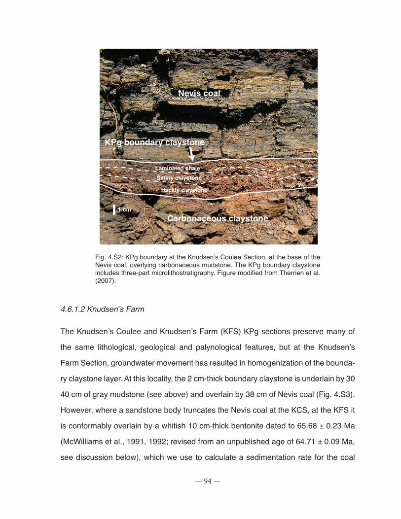
— 94 —
Fig. 4.S2: KPg boundary at the Knudsen’s Coulee Section, at the base of the Nevis coal, overlying carbonaceous mudstone. The KPg boundary claystone includes three-part microlithostratigraphy. Figure modified from Therrien et al. (2007).
4.6.1.2 Knudsen’s Farm
The Knudsen’s Coulee and Knudsen’s Farm (KFS) KPg sections preserve many of
the same lithological, geological and palynological features, but at the Knudsen’s
Farm Section, groundwater movement has resulted in homogenization of the bounda-
ry claystone layer. At this locality, the 2 cm-thick boundary claystone is underlain by 30
40 cm of gray mudstone (see above) and overlain by 38 cm of Nevis coal (Fig. 4.S3).
However, where a sandstone body truncates the Nevis coal at the KCS, at the KFS it
is conformably overlain by a whitish 10 cm-thick bentonite dated to 65.68 ± 0.23 Ma
(McWilliams et al., 1991, 1992; revised from an unpublished age of 64.71 ± 0.09 Ma,
see discussion below), which we use to calculate a sedimentation rate for the coal
1 cm
Hackly claystone
Satiny claystoneLaminated shale
Nevis coal
KPg boundary claystone
Carbonaceous claystone
Cousineau et al. -- Figure S2
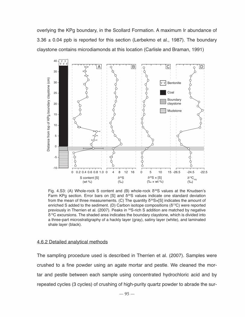
— 95 —
overlying the KPg boundary, in the Scollard Formation. A maximum Ir abundance of
3.36 ± 0.04 ppb is reported for this section (Lerbekmo et al., 1987). The boundary
claystone contains microdiamonds at this location (Carlisle and Braman, 1991)
-10
5
0
-5
10
15
20
25
30
35
Dis
tanc
e fro
m to
p of
KPg
bou
ndar
y cl
ayst
one
(cm
)
40
S content [S] (wt %)
δ34S(‰)
δ34S × [S] (‰ × wt %)
0 4 128 16 0 5 10 150 0.2 0.4 0.6 0.8 1.0 -26.5 -24.5 -22.5δ13Corg(‰)
A B C D
Bentonite
Mudstone
Coal
Boundaryclaystone
Cousineau et al. -- Figure S3
Fig. 4.S3: (A) Whole-rock S content and (B) whole-rock δ34S values at the Knudsen’s Farm KPg section. Error bars on [S] and δ34S values indicate one standard deviation from the mean of three measurements. (C) The quantity δ34S×[S] indicates the amount of enriched S added to the sediment. (D) Carbon isotope compositions (δ13C) were reported previously in Therrien et al. (2007). Peaks in 34S-rich S addition are matched by negative δ13C excursions. The shaded area indicates the boundary claystone, which is divided into a three-part microstratigraphy of a hackly layer (gray), satiny layer (white), and laminated shale layer (black).
4.6.2 Detailed analytical methods
The sampling procedure used is described in Therrien et al. (2007). Samples were
crushed to a fine powder using an agate mortar and pestle. We cleaned the mor-
tar and pestle between each sample using concentrated hydrochloric acid and by
repeated cycles (3 cycles) of crushing of high-purity quartz powder to abrade the sur-
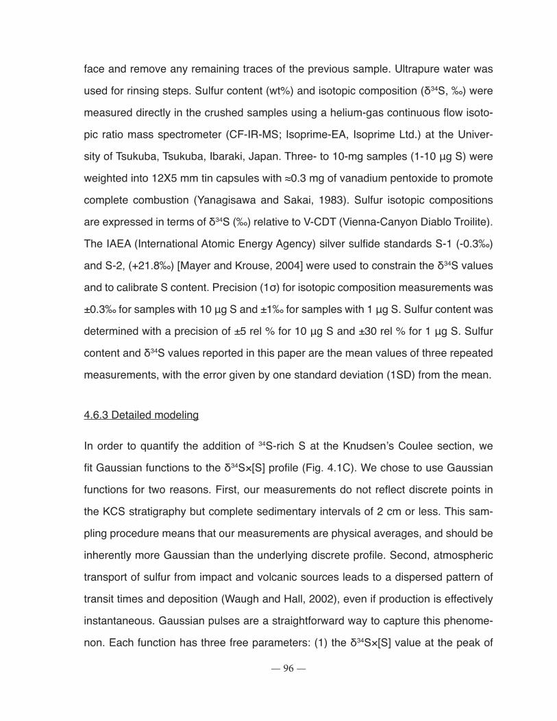
— 96 —
face and remove any remaining traces of the previous sample. Ultrapure water was
used for rinsing steps. Sulfur content (wt%) and isotopic composition (δ34S, ‰) were
measured directly in the crushed samples using a helium-gas continuous flow isoto-
pic ratio mass spectrometer (CF-IR-MS; Isoprime-EA, Isoprime Ltd.) at the Univer-
sity of Tsukuba, Tsukuba, Ibaraki, Japan. Three- to 10-mg samples (1-10 μg S) were
weighted into 12X5 mm tin capsules with ≈0.3 mg of vanadium pentoxide to promote
complete combustion (Yanagisawa and Sakai, 1983). Sulfur isotopic compositions
are expressed in terms of δ34S (‰) relative to V-CDT (Vienna-Canyon Diablo Troilite).
The IAEA (International Atomic Energy Agency) silver sulfide standards S-1 (-0.3‰)
and S-2, (+21.8‰) [Mayer and Krouse, 2004] were used to constrain the δ34S values
and to calibrate S content. Precision (1σ) for isotopic composition measurements was
±0.3‰ for samples with 10 μg S and ±1‰ for samples with 1 μg S. Sulfur content was
determined with a precision of ±5 rel % for 10 μg S and ±30 rel % for 1 μg S. Sulfur
content and δ34S values reported in this paper are the mean values of three repeated
measurements, with the error given by one standard deviation (1SD) from the mean.
4.6.3 Detailed modeling
In order to quantify the addition of 34S-rich S at the Knudsen’s Coulee section, we
fit Gaussian functions to the δ34S×[S] profile (Fig. 4.1C). We chose to use Gaussian
functions for two reasons. First, our measurements do not reflect discrete points in
the KCS stratigraphy but complete sedimentary intervals of 2 cm or less. This sam-
pling procedure means that our measurements are physical averages, and should be
inherently more Gaussian than the underlying discrete profile. Second, atmospheric
transport of sulfur from impact and volcanic sources leads to a dispersed pattern of
transit times and deposition (Waugh and Hall, 2002), even if production is effectively
instantaneous. Gaussian pulses are a straightforward way to capture this phenome-
non. Each function has three free parameters: (1) the δ34S×[S] value at the peak of
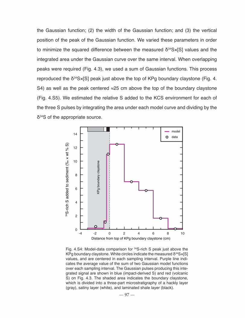
— 97 —
the Gaussian function; (2) the width of the Gaussian function; and (3) the vertical
position of the peak of the Gaussian function. We varied these parameters in order
to minimize the squared difference between the measured δ34S×[S] values and the
integrated area under the Gaussian curve over the same interval. When overlapping
peaks were required (Fig. 4.3), we used a sum of Gaussian functions. This process
reproduced the δ34S×[S] peak just above the top of KPg boundary claystone (Fig. 4.
S4) as well as the peak centered ≈25 cm above the top of the boundary claystone
(Fig. 4.S5). We estimated the relative S added to the KCS environment for each of
the three S pulses by integrating the area under each model curve and dividing by the
δ34S of the appropriate source.
Fig. 4.S4: Model-data comparison for 34S-rich S peak just above the KPg boundary claystone. White circles indicate the measured δ34S×[S] values, and are centered in each sampling interval. Purple line indi-cates the average value of the sum of two Gaussian model functions over each sampling interval. The Gaussian pulses producing this inte-grated signal are shown in blue (impact-derived S) and red (volcanic S) on Fig. 4.3. The shaded area indicates the boundary claystone, which is divided into a three-part microstratigraphy of a hackly layer (gray), satiny layer (white), and laminated shale layer (black).
-4 -2 0 2 4 6 8 100
2
4
6
8
10
12
14
Distance from top of KPg boundary claystone (cm)
34S-
rich
S ad
ded
to s
edim
ent (
‰ ×
wt %
S)
modeldata
KPg
boun
dary
cla
ysto
ne
Cousineau et al. -- Figure S4
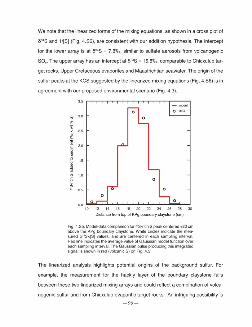
— 98 —
We note that the linearized forms of the mixing equations, as shown in a cross plot of
δ34S and 1/[S] (Fig. 4.S6), are consistent with our addition hypothesis. The intercept
for the lower array is at δ34S = 7.8‰, similar to sulfate aerosols from volcanogenic
SO2. The upper array has an intercept at δ34S = 15.8‰, comparable to Chicxulub tar-
get rocks, Upper Cretaceous evaporites and Maastrichtian seawater. The origin of the
sulfur peaks at the KCS suggested by the linearized mixing equations (Fig. 4.S6) is in
agreement with our proposed environmental scenario (Fig. 4.3).
Fig. 4.S5. Model-data comparison for 34S-rich S peak centered ≈20 cm above the KPg boundary claystone. White circles indicate the mea-sured δ34S×[S] values, and are centered in each sampling interval. Red line indicates the average value of Gaussian model function over each sampling interval. The Gaussian pulse producing this integrated signal is shown in red (volcanic S) on Fig. 4.3.
The linearized analysis highlights potential origins of the background sulfur. For
example, the measurement for the hackly layer of the boundary claystone falls
between these two linearized mixing arrays and could reflect a combination of volca-
nogenic sulfur and from Chicxulub evaporitic target rocks. An intriguing possibility is
10 12 14 16 18 20 22 24 26 28 300.0
0.5
1.0
1.5
2.0
2.5
3.0
3.5
Distance from top of KPg boundary claystone (cm)
34S-
rich
S ad
ded
to s
edim
ent (
‰ ×
wt %
S)
modeldata
Cousineau et al. -- Figure S5
— 99 —
that this sample includes a component of meteoritic sulfur (δ34S = 0‰), which would
pull the δ34S value off of upper evaporitic array. As is apparent in the mixing ana-
lysis presented in the text (Fig. 4.2), there is a hint of volcanically-derived sulfur in
samples below the boundary claystone, possibly reflecting contribution from a minor
early phase of Deccan volcanism prior to the KPg boundary.
1/[S] (wt %-1)
Who
le-ro
ck δ
34S
valu
es (‰
)
0
5
10
15
20
0 10 20 30 40
Cousineau et al. -- Figure S6
Fig. 4.S6: Linearized cross plot of δ34S values and the inverse of whole-rock S contents (1/[S]) measured at the Knudsen’s Coulee Sec-tion. The upper mixing array is consistent with S from Chicxulub tar-get rocks and end-Cretaceous seawater and evaporites (white circles). The lower mixing array is consistent with S from oxidized volcanic SO2 (gray circles). The measurement for the lowermost unit of the boundary claystone, the hackly layer (black cirle), falls between these two arrays and could reflect mixing between various sources of S, including meteo-ritic S (δ34S = 0‰), volcanogenic S and S from the Maastrichtian evapo-ritic target rocks. Error bars indicate standard deviation from the mean of three measurements. Where these are not visible, they are smaller than the symbols used.
— 100 —
4.6.4 KFS discussion
Although the Knudsen’s Farm KPg Section (KFS) preserves many of the same litho-
logical, palynological and geochemical features as the Knudsen’s Coulee Section,
the KFS boundary claystone is completely homogenized and its constituent subunits
cannot be recognized. Apparently, groundwater movement has resulted in the loss
of any microlithostratigraphy that was originally present. Because of the clear post-
depositional chemical mobility, we do not quantitatively interpret the S isotope syste-
matics at KFS. However, the S content, δ34S and 34S-rich S profiles for the KFS are
broadly comparable to those for the KCS (Figs. 4.1, 4.S3). For example, S content
and δ34S profiles are closely correlated around the boundary claystone (Fig. 4.S3A, B)
leading to a peak of 34S-rich S extending to >10 cm above the claystone (Fig. 4.S3C).
This peak is not as sharp as the corresponding feature in the KCS profile. Similarly,
while a distinct second peak of 34S-rich S is centered about 20 cm above the boun-
dary claystone in the KCS profile, the upper KFS profile shows a much more subdued
pattern of 34S addition. Within a broad region that persists over the remainder of the
section, levels of 34S-rich S are only slightly above background values (Fig. 4.S3C).
This pattern likely reflects S mobilization by groundwater flow through the sediment
as both the S contents and δ34S values are spread out over a similar vertical distance
(Fig. 4.S3A, B). In summary, we expect that profiles of S content, δ34S values, and 34S-
rich S at the KFS originally resembled those at the KCS. However, post-depositional S
transport acted as a broadband filter, destroying comparable chronologic information
at the KFS. We note that this does not seem to be the case for δ13C values in organic
matter (cf. Fig. 4.1D, Fig. 4.S3D). The C content of the Nevis Coal is much greater
than its S content, thereby making the organic δ13C record much more resistant to
resetting than the δ34S record. Both the KCS and KFS preserve δ13C minima at ≈5 cm
above the boundary claystone, supporting our application of stratigraphic timescales
calculated for KFS to the KCS.

— 101 —
4.6.5 Absolute KPg chronology
In order to compare our proposed relative environmental chronology to absolute timing
of events across the KPg boundary, we compiled age estimates of the KPg boun-
dary, Chicxulub impactites, bentonites in Western Interior sedimentary basins, and
the continental flood basalts of the main Deccan traps. Age estimates from 40Ar/39Ar
measurements were recalculated to a common age standard in order to construct a
consistent chronology (Fig. 4.S7). Here we present detailed descriptions of the com-
ponents of this chronology, explore potential pitfalls associated with the chronology,
and use it to derive a chronological calibration for the Scollard Formation in the area
of Knudsen’s T. rex Ranch.
4.6.5.1 KPg boundary
Marine paleomagnetic measurements indicate that the KPg boundary falls in the
middle the 29r magnetic polarity chron (Cande and Kent, 1995). The latest consen-
sus geologic time scale places the KPg boundary at 65.50 ± 0.30 Ma (Gradstein et
al, 2004). Cross-calibrations of orbitally tuned sedimentary cycles with high-precision 40Ar/39Ar age determinations produced a slightly older, and significantly more precise,
estimate of 65.957 ± 0.043 Ma for the KPg boundary (uncertainty is 2 standard error
[SE] on the mean; Kuiper et al., 2008; Fig. 4.S7A). A recent astronomical calibra-
tion of Maastrichtian marine cyclostratigraphic datasets (magnetic susceptibility and
grayscale measurements from Ocean Drilling Project and Deep Sea Drilling Project
cores) returned an equivalent age for the KPg boundary of 66.00 ± 0.07 Ma (Husson
et al., 2011; Fig. 4.S7A). These estimates, and consistent ages for magnetic polarity
chron boundaries (C30n/C29r - 66.30 ± 0.08 Ma, Husson et al., 2011; C29r/C29n -
65.724 ± 0.055 Ma [2SE], Kuiper et al., 2008), provide a chronological framework
for examining the absolute ages of environmental events across the KPg boundary.
The 65.957 ± 0.043 Ma age for the KPg boundary is cross calibrated to an age of
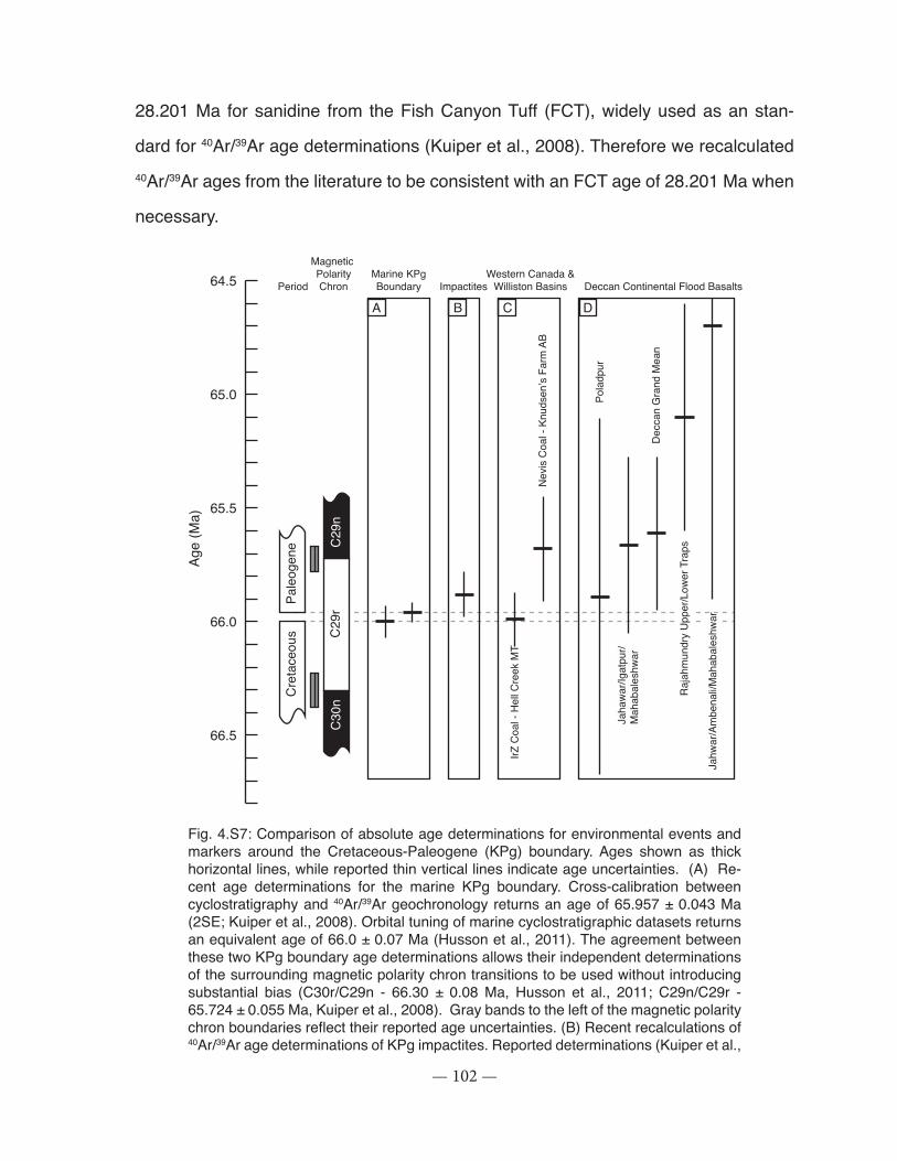
— 102 —
28.201 Ma for sanidine from the Fish Canyon Tuff (FCT), widely used as an stan-
dard for 40Ar/39Ar age determinations (Kuiper et al., 2008). Therefore we recalculated 40Ar/39Ar ages from the literature to be consistent with an FCT age of 28.201 Ma when
necessary.
Fig. 4.S7: Comparison of absolute age determinations for environmental events and markers around the Cretaceous-Paleogene (KPg) boundary. Ages shown as thick horizontal lines, while reported thin vertical lines indicate age uncertainties. (A) Re-cent age determinations for the marine KPg boundary. Cross-calibration between cyclostratigraphy and 40Ar/39Ar geochronology returns an age of 65.957 ± 0.043 Ma (2SE; Kuiper et al., 2008). Orbital tuning of marine cyclostratigraphic datasets returns an equivalent age of 66.0 ± 0.07 Ma (Husson et al., 2011). The agreement between these two KPg boundary age determinations allows their independent determinations of the surrounding magnetic polarity chron transitions to be used without introducing substantial bias (C30r/C29n - 66.30 ± 0.08 Ma, Husson et al., 2011; C29n/C29r - 65.724 ± 0.055 Ma, Kuiper et al., 2008). Gray bands to the left of the magnetic polarity chron boundaries reflect their reported age uncertainties. (B) Recent recalculations of 40Ar/39Ar age determinations of KPg impactites. Reported determinations (Kuiper et al.,
Cre
tace
ous
Pale
ogen
e
Magnetic PolarityChron
C29
rC
29n
C30
n
66.5
66.0
65.5
65.0
64.5
Jahw
ar/A
mbe
nali/
Mah
abal
eshw
ar
Jaha
war
/Igat
pur/
Mah
abal
eshw
ar
Marine KPgBoundary Deccan Continental Flood Basalts
Age
(Ma)
Raj
ahm
undr
y U
pper
/Low
er T
raps
Pola
dpur
Dec
can
Gra
nd M
ean
AImpactites
B DPeriod
IrZ C
oal -
Hel
l Cre
ek M
T
Nev
is C
oal -
Knu
dsen
’s F
arm
AB
Western Canada & Williston Basins
C
Cousineau et al. -- Figure S7

— 103 —
2008) are all consistent with a grand mean of 65.88 ± 0.10 Ma (2SE). (C) Recalculation of terrestrial KPg boundary ages from Western Interior of North America. The lowest coal in the Williston Basin (IrZ Coal) is enriched in Ir (Swisher et al., 1993). Bentonite beds within the IrZ Coal return 40Ar/39Ar ages on sanidine of 65.99 ± 0.12 Ma (2SE; Swisher et al., 1993 as recalculated in Kuiper et al., 2008). The first coal seam above the KPg boundary clay in the Western Canada Sedimentary Basin of Alberta (Nevis Coal) contains a bentonite bed characterized by a 40Ar/39Ar age of 65.68 ± 0.23 Ma (as estimated from data in McWilliams et al, 1991, 1992; Kuiper et al., 2008). (D) Recent and recalculated age determinations for Deccan Traps volcanism. Seven 40Ar/39Ar age determinations on mineral separates from samples of the Jahwar, Igatpuri, and Maha-baleshwar Formations are consistent with a single mean age of 65.66 ± 0.39 Ma (95% CI [1SE = 0.16 Ma]; recalculated from Hoffman et al., 2000). Three 40Ar/39Ar age on plagioclase mineral separates from samples of the Poladpur Formation are consistent with a single mean age of 65.89 ± 0.79 Ma (95% CI [1SE = 0.18 Ma]; recalculated from Hooper et al., 2010). Upper and lower Rajahmundry Traps are characterized by a single mean age of 65.1 ± 0.5 Ma (95 CI; recalculated from mean age of 12 ana-lyses of 8 samples reported in Knight et al., 2003). Ages determined with the 40K/40Ar method on seven samples from the Jahwar, Igatpuri, Ambenali, and Mahabaleshwar Formations are consistent with a single mean value of 64.7 ± 1.2 Ma (2SE; Chenet et al., 2007). Uncertainty was assigned under the assumption that 1σ values reported for these samples refer to the standard error on the reported mean values (Chenet et al., 2007).
4.6.5.2 Impactites
Relative to an FCT age of 28.201 Ma, impactites associated with the KPg impact event
(tektites from Beloc Haiti [Izett et al., 1991; Swisher et al., 1992; Dalyrymple et al.,
1993], microtektites from Arroyo el Mimbral, Mexico [Swisher et al., 1992], and glassy
melt rock C-1 from Chicxulub crater [Swisher et al., 1992]) yield a sample distribution
of 40Ar/39Ar ages that are consistent with a single mean value (Kuiper et al., 2008). The
grand mean of these ages is 65.88 ± 0.10 Ma (Fig. 4.S7B), where the uncertainty is
calculated as the 95% confidence interval (CI) on the mean accounting for the effects
of small-number statistics (Mahon, 1996). The associated SE is 0.04 Ma.
4.6.5.3 Western Interior sedimentary basins
Abundant and well-studied pollen, plant, and vertebrate fossils constrain the paleon-
tological expression of the terrestrial KPg boundary in sedimentary strata of the North
American midcontinent (Nichols and Johnson, 2008; Archibald, 2011). Sedimentary
— 104 —
basins of the North American midcontinent also preserve a broadly distributed, dis-
tinctive stratigraphic horizon at the KPg boundary – the ‘boundary claystone’ – that is
taken to represent fallout from a KPg impact event (Bohor et al., 1984). A consistent
three-part microstratigraphy is often found within the boundary claystone (Sweet et
al., 1999), and is well illustrated by the boundary clay found in the Knudsen’s Coulee
section in the Scollard Formation, AB (Fig. 4.S2). Paleomagnetic measurements indi-
cate that the KPg boundary in these sections occurs within magnetic polarity chron
29r (Swisher et al., 1993), consistent with the marine magnetostratigraphic record.
Widespread coals with interbedded bentonites enable a highly resolved absolute chro-
nology for Western Interior sedimentary basins (Swisher et al., 1993). A maximum age
for the terrestrial KPg boundary is constrained by a 40Ar/39Ar age of 65.99 ± 0.12 Ma
(2SE; Swisher et al., 1993, recalculated based on a FCT age of 28.201 Ma in Kuiper et
al., 2008; Fig. 4.S7C) measured on sanidine from bentonites within the IrZ coal (Wil-
liston Basin, Hell Creek, Montana). Unpublished high-precision 40Ar/39Ar ages from
the first bentonite above the boundary clay (conformably overlying the Nevis Coal) at
Knudsen’s Farm, AB are 0.20 ± 0.15 Ma older than Beloc tektites from Haiti (uncer-
tainty is 2SE on the difference between two mean values; McWilliams et al., 1991,
1992). Taking the grand mean of impactite 40Ar/39Ar ages (65.88 ± 0.10 Ma [95% CI;
1SE = 0.04 Ma], as described in the preceding section) to reflect the age of the Beloc
tektites, the relative timing suggests that the bentonite overlying the Nevis Coal for-
med at 65.68 ± 0.23 Ma (2SE; Fig. 4.S7C).
4.6.5.4 Deccan Traps continental flood basalts
The Deccan Traps preserve a limited number of magnetic reversals, long hinting at
a rapid eruption history (McElhinny, 1968; Wensink and Klootwijk, 1971). Paleonto-
logical and geochronological observations suggest that the Deccan eruptions span
the KPg boundary, indicating that transition between magnetic polarity chrons C29r
— 105 —
and C29n is the most likely candidate for the major magnetic reversal recorded in
the Deccan magnetostratigraphy (Courtillot et al., 1986). Early syntheses of geologi-
cal, paleontological, geochronological and paleomagnetic datasets concluded that a
dominant majority of the Deccan eruptions took place within magnetic polarity chron
C29r (Vandamme et al., 1991), a result supported by recent detailed interdisciplinary
reexaminations (Fig. 4.S8; Chenet et al., 2009; Jaye et al., 2009). Aside from a minor,
geographically restricted early phase of volcanism occurring around the transition
between magnetic polarity chrons C30r and C30n, current interpretations call on two
brief, intense, and closely paced pulses of Deccan eruptions (Chenet et al., 2009).
Much of this main Deccan eruptive phase occurs during magnetic polarity chron C29r,
with the transition between magnetic polarity chrons C29r and C29n occurring during
the emplacement of the Mahabaleshwar Formation (Fig. 4.S8; Chenet et al., 2009;
Jaye et al., 2009). In fact, eruptive accounting suggests that more than 85% of the
main Deccan eruptive phase occurred during magnetic polarity chron C29r (Self et al.,
2006), which lasts 0.576 ± 0.097 (2SE) Myrs within the chronological framework used
here (Fig. 4.S7).
This timing is supported by recent age determinations on stratigraphically control-
led Deccan Trap flows and their possible far-field equivalents. Three samples of the
Poladpur Formation (Fig. 4.S8), at the base of the uppermost and most voluminous
collection of Deccan flows (the Wai subgroup; Self et al., 2006), are consistent with
a single mean 40Ar/39Ar age of 65.89 ± 0.79 Ma (95% CI [1SE = 0.18 Ma]; Hooper
et al., 2010, recalculated ages based on an age of GA1550 = 99.416 Ma relative to
FCT = 28.201 Ma; Kuiper et al., 2008; Fig. 4.S7D). This temporal consistency appears
to extend through the Deccan Traps as a whole. Samples from the lower and upper
main Traps (Jahwar/Igatpuri/Mahabaleshwar Formations; Fig. 4.S8) are consistent
with a single mean 40Ar/39Ar age of 65.66 ± 0.39 (95% CI [1SE = 0.16 Ma]; Hofmann
et al., 2000, recalculated ages based on an age of Hb3gr = 1079.23 Ma relative to
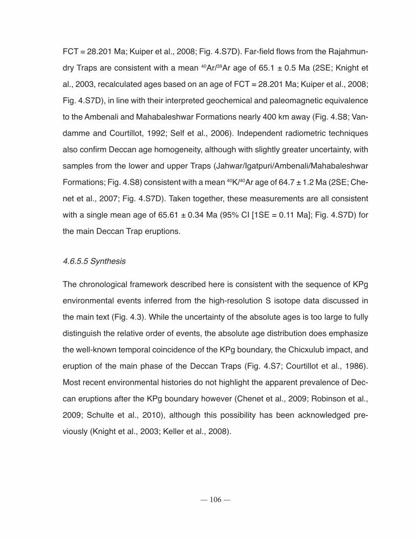
— 106 —
FCT = 28.201 Ma; Kuiper et al., 2008; Fig. 4.S7D). Far-field flows from the Rajahmun-
dry Traps are consistent with a mean 40Ar/39Ar age of 65.1 ± 0.5 Ma (2SE; Knight et
al., 2003, recalculated ages based on an age of FCT = 28.201 Ma; Kuiper et al., 2008;
Fig. 4.S7D), in line with their interpreted geochemical and paleomagnetic equivalence
to the Ambenali and Mahabaleshwar Formations nearly 400 km away (Fig. 4.S8; Van-
damme and Courtillot, 1992; Self et al., 2006). Independent radiometric techniques
also confirm Deccan age homogeneity, although with slightly greater uncertainty, with
samples from the lower and upper Traps (Jahwar/Igatpuri/Ambenali/Mahabaleshwar
Formations; Fig. 4.S8) consistent with a mean 40K/40Ar age of 64.7 ± 1.2 Ma (2SE; Che-
net et al., 2007; Fig. 4.S7D). Taken together, these measurements are all consistent
with a single mean age of 65.61 ± 0.34 Ma (95% CI [1SE = 0.11 Ma]; Fig. 4.S7D) for
the main Deccan Trap eruptions.
4.6.5.5 Synthesis
The chronological framework described here is consistent with the sequence of KPg
environmental events inferred from the high-resolution S isotope data discussed in
the main text (Fig. 4.3). While the uncertainty of the absolute ages is too large to fully
distinguish the relative order of events, the absolute age distribution does emphasize
the well-known temporal coincidence of the KPg boundary, the Chicxulub impact, and
eruption of the main phase of the Deccan Traps (Fig. 4.S7; Courtillot et al., 1986).
Most recent environmental histories do not highlight the apparent prevalence of Dec-
can eruptions after the KPg boundary however (Chenet et al., 2009; Robinson et al.,
2009; Schulte et al., 2010), although this possibility has been acknowledged pre-
viously (Knight et al., 2003; Keller et al., 2008).
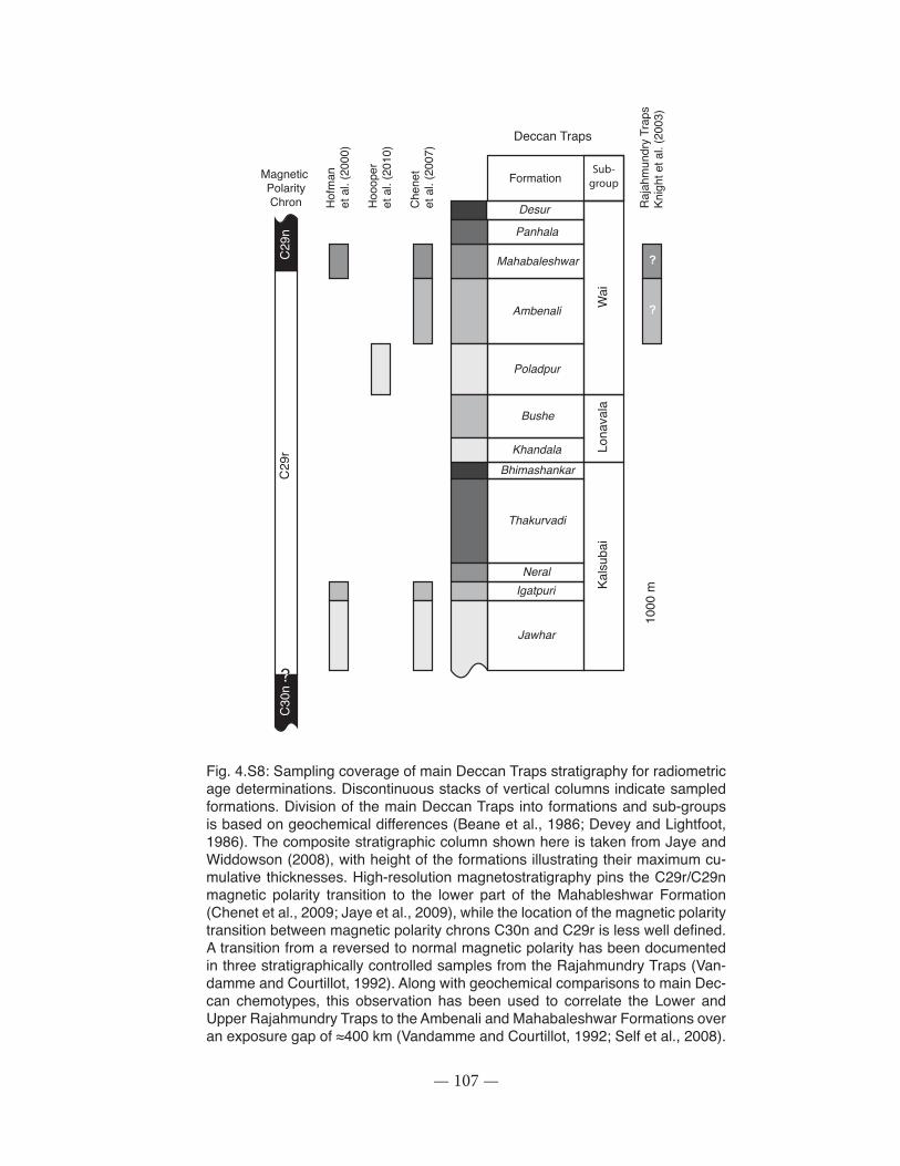
— 107 —
Deccan Traps
C29
rC
29n
C30
n
Magnetic PolarityChron
Jawhar
IgatpuriNeral
Thakurvadi
BhimashankarKhandala
Bushe
Poladpur
Ambenali
Mahabaleshwar
Panhala
Wai
Lona
vala
Kals
ubai
FormationSub-
group
Hof
man
et a
l. (2
000)
Hoo
oper
et a
l. (2
010)
Che
net
et a
l. (2
007)
1000
mR
ajah
mun
dry
Trap
sKn
ight
et a
l. (2
003)
?
?
Desur
Cousineau et al. -- Figure S8
Fig. 4.S8: Sampling coverage of main Deccan Traps stratigraphy for radiometric age determinations. Discontinuous stacks of vertical columns indicate sampled formations. Division of the main Deccan Traps into formations and sub-groups is based on geochemical differences (Beane et al., 1986; Devey and Lightfoot, 1986). The composite stratigraphic column shown here is taken from Jaye and Widdowson (2008), with height of the formations illustrating their maximum cu-mulative thicknesses. High-resolution magnetostratigraphy pins the C29r/C29n magnetic polarity transition to the lower part of the Mahableshwar Formation (Chenet et al., 2009; Jaye et al., 2009), while the location of the magnetic polarity transition between magnetic polarity chrons C30n and C29r is less well defined. A transition from a reversed to normal magnetic polarity has been documented in three stratigraphically controlled samples from the Rajahmundry Traps (Van-damme and Courtillot, 1992). Along with geochemical comparisons to main Dec-can chemotypes, this observation has been used to correlate the Lower and Upper Rajahmundry Traps to the Ambenali and Mahabaleshwar Formations over an exposure gap of ≈400 km (Vandamme and Courtillot, 1992; Self et al., 2008).
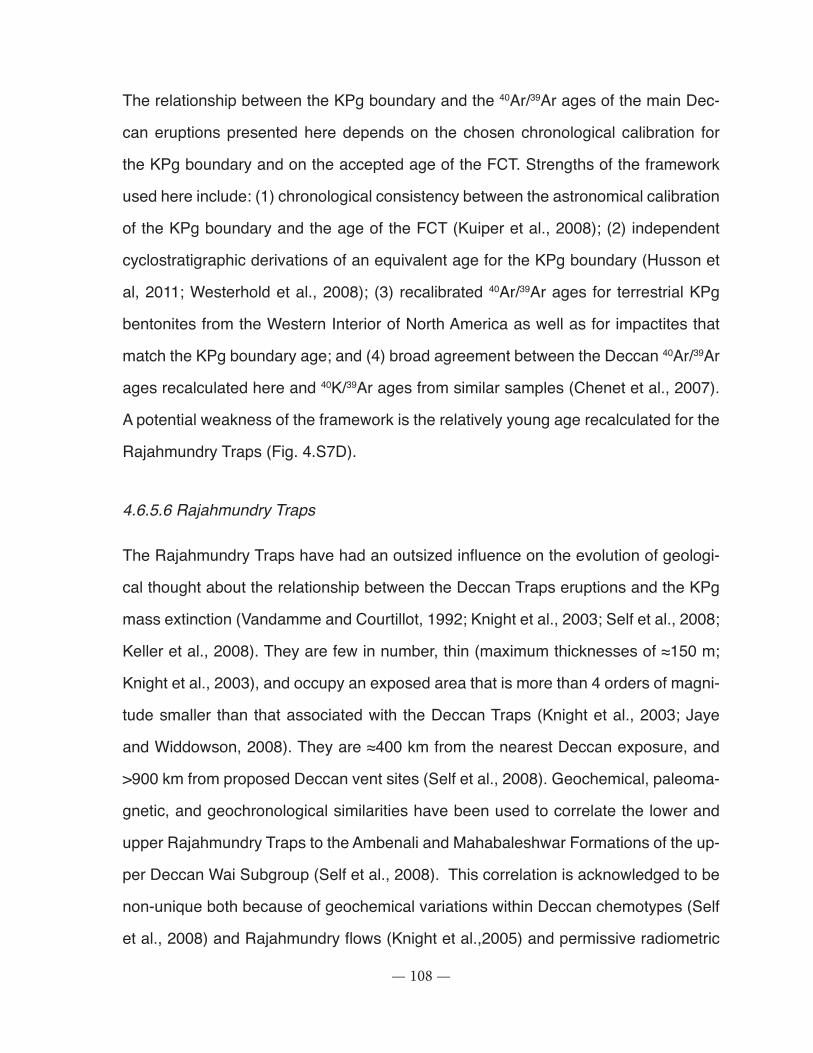
— 108 —
The relationship between the KPg boundary and the 40Ar/39Ar ages of the main Dec-
can eruptions presented here depends on the chosen chronological calibration for
the KPg boundary and on the accepted age of the FCT. Strengths of the framework
used here include: (1) chronological consistency between the astronomical calibration
of the KPg boundary and the age of the FCT (Kuiper et al., 2008); (2) independent
cyclostratigraphic derivations of an equivalent age for the KPg boundary (Husson et
al, 2011; Westerhold et al., 2008); (3) recalibrated 40Ar/39Ar ages for terrestrial KPg
bentonites from the Western Interior of North America as well as for impactites that
match the KPg boundary age; and (4) broad agreement between the Deccan 40Ar/39Ar
ages recalculated here and 40K/39Ar ages from similar samples (Chenet et al., 2007).
A potential weakness of the framework is the relatively young age recalculated for the
Rajahmundry Traps (Fig. 4.S7D).
4.6.5.6 Rajahmundry Traps
The Rajahmundry Traps have had an outsized influence on the evolution of geologi-
cal thought about the relationship between the Deccan Traps eruptions and the KPg
mass extinction (Vandamme and Courtillot, 1992; Knight et al., 2003; Self et al., 2008;
Keller et al., 2008). They are few in number, thin (maximum thicknesses of ≈150 m;
Knight et al., 2003), and occupy an exposed area that is more than 4 orders of magni-
tude smaller than that associated with the Deccan Traps (Knight et al., 2003; Jaye
and Widdowson, 2008). They are ≈400 km from the nearest Deccan exposure, and
>900 km from proposed Deccan vent sites (Self et al., 2008). Geochemical, paleoma-
gnetic, and geochronological similarities have been used to correlate the lower and
upper Rajahmundry Traps to the Ambenali and Mahabaleshwar Formations of the up-
per Deccan Wai Subgroup (Self et al., 2008). This correlation is acknowledged to be
non-unique both because of geochemical variations within Deccan chemotypes (Self
et al., 2008) and Rajahmundry flows (Knight et al.,2005) and permissive radiometric
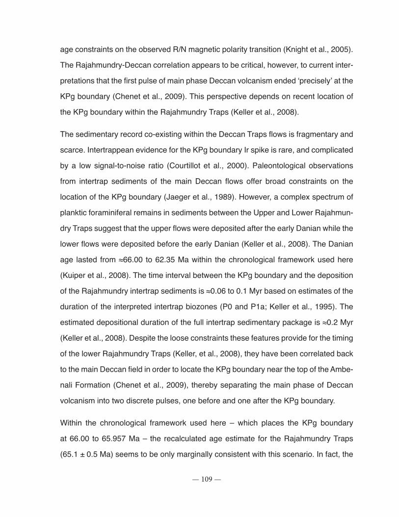
— 109 —
age constraints on the observed R/N magnetic polarity transition (Knight et al., 2005).
The Rajahmundry-Deccan correlation appears to be critical, however, to current inter-
pretations that the first pulse of main phase Deccan volcanism ended ‘precisely’ at the
KPg boundary (Chenet et al., 2009). This perspective depends on recent location of
the KPg boundary within the Rajahmundry Traps (Keller et al., 2008).
The sedimentary record co-existing within the Deccan Traps flows is fragmentary and
scarce. Intertrappean evidence for the KPg boundary Ir spike is rare, and complicated
by a low signal-to-noise ratio (Courtillot et al., 2000). Paleontological observations
from intertrap sediments of the main Deccan flows offer broad constraints on the
location of the KPg boundary (Jaeger et al., 1989). However, a complex spectrum of
planktic foraminiferal remains in sediments between the Upper and Lower Rajahmun-
dry Traps suggest that the upper flows were deposited after the early Danian while the
lower flows were deposited before the early Danian (Keller et al., 2008). The Danian
age lasted from ≈66.00 to 62.35 Ma within the chronological framework used here
(Kuiper et al., 2008). The time interval between the KPg boundary and the deposition
of the Rajahmundry intertrap sediments is ≈0.06 to 0.1 Myr based on estimates of the
duration of the interpreted intertrap biozones (P0 and P1a; Keller et al., 1995). The
estimated depositional duration of the full intertrap sedimentary package is ≈0.2 Myr
(Keller et al., 2008). Despite the loose constraints these features provide for the timing
of the lower Rajahmundry Traps (Keller, et al., 2008), they have been correlated back
to the main Deccan field in order to locate the KPg boundary near the top of the Ambe-
nali Formation (Chenet et al., 2009), thereby separating the main phase of Deccan
volcanism into two discrete pulses, one before and one after the KPg boundary.
Within the chronological framework used here – which places the KPg boundary
at 66.00 to 65.957 Ma – the recalculated age estimate for the Rajahmundry Traps
(65.1 ± 0.5 Ma) seems to be only marginally consistent with this scenario. In fact, the
— 110 —
recalculated age suggests that the proposed R/N magnetic polarity transition in the
Rajahmundry Traps reflects the C28r/C28n transition (64.698 ± 0.055 Ma; Kuiper et
al., 2008) rather than the C29r/C29n transitions of the main Deccan field. This sugges-
tion is not new (Knight et al., 2005). However even the existence of a major polarity
transition must be a tentative interpretation given the limited number of stratigraphical-
ly controlled paleomagnetic measurements from the Rajahmundry Traps (3 samples;
Vandamme and Courtillot, 1992). Although a younger age of the Rajahmundry Traps
is not supported by the biostratigraphic interpretations discussed in the preceding
paragraph, alternative planktic foraminiferal zonation schemes exist (Arenillas et al.,
2006; Molina et al., 2009). Within these schemes, some of the index species within
the Rajahmundry intertrap sediments apparently have non-overlapping stratigraphic
ranges. The resulting interpretation would be that much of the Rajahmundry intertrap
planktic foraminiferal record is reworked and potentially younger than early Danian.
A reworked component of the Rajahmundry intertrap planktic foraminiferal population
has been identified (Keller et al., 2008).
Clearly the relationships among the Rajahumundry Traps, the Deccan Traps, and
environmental events across the KPg boundary are complex and unsettled though the
statistical synchroneity of the Rajahumundry and Deccan eruptions (Fig. 4.S7D) does
place limits on the timeframe over which these relationships must play out.
4.6.5.7 Implications
Aside from the broad implications of the coincidence among the Chicxulub impact,
eruption of the Deccan Traps, and the biotic turnover indicated by the KPg boundary,
the chronological framework discussed here has specific implications for the timing of
these events as represented in the Knudsen’s Coulee (AB) section.
Like many of terrestrial KPg boundaries in the North American mid-continent (Nichols
— 111 —
and Johnson, 2008), the KPg boundary at Knudsen’s Coulee is defined by a boundary
claystone with a well-defined microstratigraphy, coincident with Ir enrichment and a
spike in fern spore abundances (Sweet et al., 1999). The Nevis Coal overlies the
boundary claystone at Knudsen’s Coulee (Sweet et al., 1999). Paleomagnetic com-
pilations from various KPg sections across the Western Canada sedimentary basin
in Alberta indicate that the KPg boundary here occurs within magnetic polarity chron
C29r (Lerbekmo and Braman, 2002). Like many terrestrial and marine KPg sections
(e.g., Lerbekmo, 1999; Westerhold et al., 2008; Husson et al., 2011), the distance
from the KPg boundary to the C29r/C29n magnetic polarity transition is less than
the distance from the C30n/C29r magnetic polarity transition to the KPg boundary
(Lerbekmo and Coulter, 1985). Condensed intervals after the KPg boundary are not
uncommon in marine sections (Westerhold et al., 2008), and may represent a unique
sedimentary response to the KPg boundary event. Conformable contacts across the
KPg boundary at Knudsen’s Coulee (Therrien et al, 2007) imply that this youngwards
shift results from lower sedimentation rates towards the end of magnetic polarity chron
C29r, rather than from any missing depositional intervals. Together with the synchro-
nous deposition of the KPg boundary claystone throughout the Western Interior, these
features suggest that the best estimate of the age of the KPg boundary at Knudsen’s
Coulee is the 65.99 ± 0.12 Ma age of the IrZ Coal from the Hell Creek area, Montana
(Swisher et al., 1993 as recalculated in Kuiper et al., 2008).
There are no direct age measurements from the Knudsen’s Coulee section. However,
a nearby section (Knudsen’s Farm, 2.5 km away) preserves many of the same geo-
logical, paleontological, and geochemical features as Knudsen’s Coulee (Therrien et
al., 2007). A bentonite in the Nevis Coal here has a 40Ar/39Ar age of 65.68 ± 0.23 Ma
(McWilliams et al., 1991, 1992; estimated as described previously). This implies that
the 38 cm of sedimentary rock (Therrien et al., 2007) between the top of boundary
claystone and the first bentonite in the Nevis Coal represents 0.31 ± 0.26 Myr (2SE).

— 112 —
The stratigraphic chronological calibration at Knudsen’s Farm is 0.12 ± 0.10 cm/kyr
(2SE). Although δ13Corg profiles at Knudsen’s Farm are slightly more dispersed than at
Knudsen’s Coulee, in keeping with the greater amount of diagenetic alteration seen
at Knudsen’s Farm, the minimum in both profiles occurs within the sample taken from
4-6 cm above the top of the boundary claystone (Therrien et al., 2007). This implies
that sedimentation rates at the two sites were equivalent, and we take 0.12 ± 0.10 cm/
kyr as our best estimate of the stratigraphic chronological calibration at Knudsen’s
Coulee. The 30 cm of sedimentary rock in our section above the boundary claystone
at Knudsen’s Coulee therefore represents ≈245 ± 205 kyr (2SE). We use this estimate
to provide a timescale for the environmental events revealed by our S isotope profile.
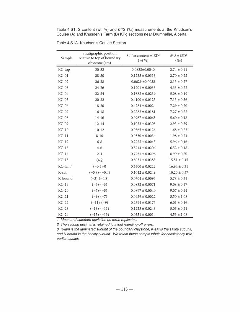
— 113 —
Table 4.S1: S content (wt. %) and δ34S (‰) measurements at the Knudsen’s Coulee (A) and Knusden’s Farm (B) KPg sections near Drumheller, Alberta.
Table 4.S1A. Knudsen’s Coulee Section
SampleStratigraphic position
relative to top of boundary claystone (cm)
Sulfur content ±1SD1
(wt %)δ34S ±1SD1
(‰)
KC-top 30-32 0.0838±0.0040 2.74 ± 0.41KC-01 28-30 0.1235 ± 0.0313 2.70 ± 0.22KC-02 26-28 0.0629 ±0.0038 2.13 ± 0.27KC-03 24-26 0.1201 ± 0.0033 4.33 ± 0.22KC-04 22-24 0.1682 ± 0.0239 5.08 ± 0.19KC-05 20-22 0.4100 ± 0.0123 7.13 ± 0.36KC-06 18-20 0.4284 ± 0.0024 7.29 ± 0.20KC-07 16-18 0.2782 ± 0.0181 7.27 ± 0.22KC-08 14-16 0.0967 ± 0.0065 5.60 ± 0.18KC-09 12-14 0.1053 ± 0.0308 2.93 ± 0.59KC-10 10-12 0.0565 ± 0.0126 1.68 ± 0.25KC-11 8-10 0.0330 ± 0.0034 1.98 ± 0.74KC-12 6-8 0.2725 ± 0.0043 5.96 ± 0.16KC-13 4-6 0.8714 ± 0.0206 6.52 ± 0.18KC-14 2-4 0.7751 ± 0.0296 8.99 ± 0.20KC-15 0-2 0.8031 ± 0.0383 15.51 ± 0.45
KC-lam3 (−0.4)-0 0.6500 ± 0.0222 16.94 ± 0.31K-sat (−0.8)-(−0.4) 0.1042 ± 0.0249 10.20 ± 0.57K-bound (−3)-(−0.8) 0.0704 ± 0.0093 5.78 ± 0.31KC-19 (−5)-(−3) 0.0832 ± 0.0071 9.08 ± 0.47KC-20 (−7)-(−5) 0.0897 ± 0.0040 9.07 ± 0.44KC-21 (−9)-(−7) 0.0459 ± 0.0022 5.50 ± 1.08KC-22 (−11)-(−9) 0.2394 ± 0.0175 6.01 ± 0.16KC-23 (−13)-(−11) 0.1223 ± 0.0243 5.05 ± 0.24KC-24 (−15)-(−13) 0.0351 ± 0.0014 4.53 ± 1.08
1. Mean and standard deviation on three replicates.2. The second decimal is retained to avoid rounding-off errors.3. K-lam is the laminated subunit of the boundary claystone, K-sat is the satiny subunit, and K-bound is the hackly subunit. We retain these sample labels for consistency with earlier studies.
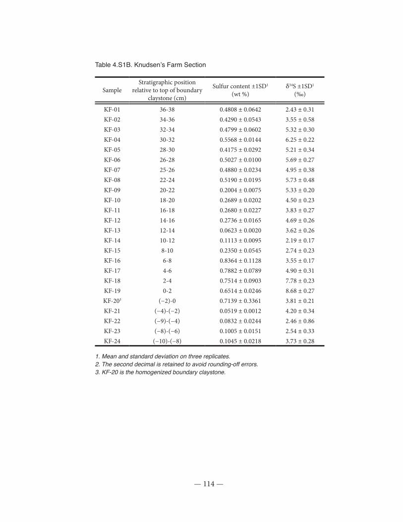
— 114 —
Table 4.S1B. Knudsen’s Farm Section
SampleStratigraphic position
relative to top of boundary claystone (cm)
Sulfur content ±1SD1
(wt %)δ34S ±1SD1
(‰)
KF-01 36-38 0.4808 ± 0.0642 2.43 ± 0.31KF-02 34-36 0.4290 ± 0.0543 3.55 ± 0.58KF-03 32-34 0.4799 ± 0.0602 5.32 ± 0.30KF-04 30-32 0.5568 ± 0.0144 6.25 ± 0.22KF-05 28-30 0.4175 ± 0.0292 5.21 ± 0.34KF-06 26-28 0.5027 ± 0.0100 5.69 ± 0.27KF-07 25-26 0.4880 ± 0.0234 4.95 ± 0.38KF-08 22-24 0.5190 ± 0.0195 5.73 ± 0.48KF-09 20-22 0.2004 ± 0.0075 5.33 ± 0.20KF-10 18-20 0.2689 ± 0.0202 4.50 ± 0.23KF-11 16-18 0.2680 ± 0.0227 3.83 ± 0.27KF-12 14-16 0.2736 ± 0.0165 4.69 ± 0.26KF-13 12-14 0.0623 ± 0.0020 3.62 ± 0.26KF-14 10-12 0.1113 ± 0.0095 2.19 ± 0.17KF-15 8-10 0.2350 ± 0.0545 2.74 ± 0.23KF-16 6-8 0.8364 ± 0.1128 3.55 ± 0.17KF-17 4-6 0.7882 ± 0.0789 4.90 ± 0.31KF-18 2-4 0.7514 ± 0.0903 7.78 ± 0.23KF-19 0-2 0.6514 ± 0.0246 8.68 ± 0.27KF-203 (−2)-0 0.7139 ± 0.3361 3.81 ± 0.21KF-21 (−4)-(−2) 0.0519 ± 0.0012 4.20 ± 0.34KF-22 (−9)-(−4) 0.0832 ± 0.0244 2.46 ± 0.86KF-23 (−8)-(−6) 0.1005 ± 0.0151 2.54 ± 0.33KF-24 (−10)-(−8) 0.1045 ± 0.0218 3.73 ± 0.28
1. Mean and standard deviation on three replicates.2. The second decimal is retained to avoid rounding-off errors.3. KF-20 is the homogenized boundary claystone.
— 115 —
References
Achenbach-Richter, L., Stetter, K.O., and Woese, C.R. 1987. A possible biochemical
missing link among archaebacteria. Nature, 327: 348-349.
Alexander, P.O. 1976. Age and duration of Deccan volcanism. K-Ar evidence. Geolo-
gical Society of India Memoir, 3: 244-258.
Alt, D., Sears, J.M., and Hyndman, D.W. 1988. Terrestrial Maria: The origins of large
basalt plateaus, hotspot tracks and spreading ridges. The Journal of Geology, 96:
647-662.
Alvarez, L.W., Alvarez, W., Asaro, F., and Michel, H.V. 1980. Extraterrestrial cause for
the Cretaceous-Tertiary extinction. Science, 208: 1095–1108.
Alvarez, L.W., Alvarez, W., Asaro, F. and Michel, H.V., 1982. Current status of the
impact theory for the terminal Cretaceous extinction. Geological Society of America
Special Paper, 190: 305-315.
Alvarez, W., Claeys, P., and Kieffer, S.W. 1995. Emplacement of Cretaceous-Tertiary
boundary shocked quartz from Chicxulub Crater. Science, 269: 930-935.
Anbar, A.D., and Knoll, A.H. 2002. Proterozoic ocean chemistry and evolution: A bioi-
norganic bridge? Science, 297: 1137-1142.
Aneja, V.P., and Cooper, W.J. 1989. Biogenic sulfur emissions: A review. pp. 2-13 In:
Saltzmann, E.S., and Cooper, W.J. (Eds.). Biogenic sulfur in the environment. ACS
Symposium Series 393. American Chemical Society, Washington, D.C. 572 p.
Anderson, R.R., and Hartung, J. 1992. The Manson impact structure; Its contribution
to impact materials at the Cretaceous/Tertiary Boundary. Proceedings of Lunar and
Planetary Science, 22: 101-110.

— 116 —
Andreae, M.O., and Barnard, W.R. 1984. The marine chemistry of dimethylsulfide.
Marine Chemistry, 14: 267-279.
Angert, A., Rachmilevitch, S., Barkan, E., Luz, B. 2003. Effects of photorespiration, the
cytochrome pathway, and the alternative pathway on the triple isotopic composition
of atmospheric O2. Global Biogeochemical Cycles, 17. DOI:10.1029/2002GB001933.
Archibald, J.D. 2011. Extinction and radiation: how the fall of dinosaurs led to the rise
of mammals. Johns Hopkins University Press, Baltimore. 108 p.
Arenillas, I., Arz, J., Grajales-Nishimura, J., Murillo-Muneton, G., Alvarez, W., Camar-
go-Zanoguera, A., Molina, E., and Rosales-Dominguez, C. 2006. Chicxulub impact
event is Cretaceous/Paleogene boundary in age: New micropaleontological evidence.
Earth and Planetary Science Letters, 249: 241-257.
Arens, N.C., and Jahren, A.H. 2000. Carbon isotopic excursion in atmospheric CO2 at
the Cretaceous-Tertiary boundary: Evidence from terrestrial sediments. Palaios, 15:
14-322.
Bajpai, S, and Prasad, G.V.R. 2000. Cretaceous age for Ir-rich Deccan intertrappean
deposits: palaeontological evidence from Anjar, western India. Journal of the Geologi-
cal Society, London, 157: 257-260.
Bak, F., and Pfennig, N. 1987. Chemolithotrophic growth of Desulfovibrio-Sulfodismu-
tans sp-nov by disproportionation of inorganic sulfur compounds. Archives of Micro-
biology, 147: 184–189.
Beane, J.E., Turner, C.A., Hooper, P.R., Subbarao, K.V., and Walsh, J.N. 1986. Stra-
tigraphy, composition and form of the Deccan basalts, Western Ghats, India. Bulletin
of Volcanology, 48: 61-63.
Beaudoin, G., Taylor, B.E., Rumble III, D., and Thiemens, M. 1994. Variations in the
— 117 —
sulfur isotope composition of troilite from the Cañon Diablo iron meteorite. Geochi-
mica et Cosmochimica Acta, 56: 2839.
Beerling, D.J., Lomax, B.H., Upchurch, G.R.Jr., Nichols, D.J., Pillmore, C.L., Handley,
L.L., and Scrimgeour, C.M. 2001. Evidence for the recovery of terrestrial ecosystems
ahead of marine primary production following a production biotic crisis at the Creta-
ceous-Tertiary boundary. Journal of the Geological Society, London, 158: 737-740.
Bekki, S. 1995. Oxidation of volcanic SO2: A sink for stratospheric OH and H2O. Geo-
physical Research Letters, 22: 913-916.
Berner, R.A. 1984. Sedimentary pyrite formation; An update. Geochimica et Cosmo-
chimica Acta, 48: 605–615.
Bhandari, N., Shukla, P.N., Ghevariya, Z.G., and Sundaram, S.M. 1995. Impact did
not trigger Deccan volcanism: Evidence from Anjar K/T boundary intertrappean sedi-
ments. Geophysical Research Letters, 22: 433-436.
Bigeleisen J. 1965. Chemistry of isotopes. Science, 147: 463-471.
Blum, J.D., and Chamberlain, C.P. 1992. Oxygen isotope constraints on the origin of
impact glasses from the Cretaceous-Tertiary boundary. Science, 257: 1104-1107.
Bohor, B.F., Foord, E.E., Modreski, P.J., and Triplehorn, D.M. 1984. Mineralogic evi-
dence for an impact event at the Cretaceous-Tertiary boundary. Science, 224: 867-
869.
Bolliger, C., Schroth, M.H., Bernasconi, S.M., Kleikemper, J., and Zeyer, J. 2001.
Sulfur isotope fractionation during microbial sulfate reduction by toluene-degrading
bacteria. Geochimica et Cosmochimica Acta, 65: 3289-3298.
Bose, M.K. 1972. Deccan basalts. Lithos, 5:131–145

— 118 —
Bottomley, R. J., Grieve, R., York, D., and Masaitis, V. 1997. The age of the Popigai
impact event and its relation to events at the Eocene/Oligocene boundary. Nature,
388: 365-368.
Bottomley, R. J., and York, D. 1989. The dating of impact melt rocks using the 40Ar-39Ar
method. Lunar and Planetary Science, XX: 101-102.
Bottomley, R. J., York, D., and Grieve, R.A.F. 1993. Age of Popigai impact event using
the 40Ar-39Ar method. Lunar and Planetary Science XXIV: p. 161.
Boudreau, B.P., and Westrich, J.T. 1984. The dependence of bacterial sulfate reduc-
tion on sulfate concentration in marine sediments. Geochimica et Cosmochimca Acta,
48: 2503–2516.
Bradford, M. 1976. A rapid and sensitive method for the quantitation of microgram
quantities of protein utilizing the principle of protein-dye binding. Analytical Bioche-
mistry, 72: 248-254.
Brasseur, G.P., Orlando, J.J. and Tyndall, G.S. (Editors). 1999. Atmospheric chemistry
and global change. Oxford University Press, New York. 654 p.
Brimblecombe, P., Hammer, C., Rodhe, H., Ryaboshapko, A., and Boutron, C.F.
1989. Human influence on the sulphur cycle. pp. 77-121 In: Brimblecombe, P., and
Lein, A.Y. (Eds.). Evolution of the global biogeochemical sulphur cycle. SCOPE 39.
Wiley, Chichester. 241 pp.
Brüchert, V., Knoblauch, C., and Jørgensen, B.B. 2001. Controls on stable sulfur iso-
tope fractionation during bacterial sulfate reduction in Arctic sediments. Geochimica
and Cosmochimica Acta, 65: 763-776.
Brunner, B., and Bernasconi, S.M. 2005. A revised isotope fractionation model for
dissimilatory sulfate reduction in sulfate reducing bacteria. Geochimica and Cosmo-
— 119 —
chimica Acta, 69: 4759-4771.
Brunner, B., Bernasconi, S.M., Kleikemper, J., and Schroth, M. H. 2005. A model for
oxygen and sulfur isotope fractionation in sulfate during bacterial sulfate reduction
processes. Geochimica et Cosmochimica Acta, 69: 4773-4785.
Buick, R., and Dunlop, J.S.R. 1990. Evaporitic sediments of early Archaean age from
the Warrawoona group, North Pole. Sedimentology, 37: 247–277.
Cameron, E.M. 1982. Sulphate and sulphate reduction in early Precambrian oceans.
Nature, 296: 145-148.
Cande, S.C., and Kent, D.V. 1995. Revised calibration of the geomagnetic polarity
timescale for the Late Cretaceous and Cenozoic. Journal of Geophysical Research,
100: 6093-6096.
Canfield, D.E. 1993. Organic matter oxidation in marine sediments, pp. 333-363. In:
Wollast, R., Mackenzie, F.T., and Chou, L. (Eds.) Interactions of C, N, P and S biogeo-
chemical cycles. Springer, Berlin. 521 p.
Canfield, D.E. 2001. Isotope fractionation by natural populations of sulfate-reducing
bacteria. Geochimica et Cosmochimica Acta, 65: 1117-1124.
Canfield, D.E., Habicht, K., and Thamdrup, B. 2000. The Archean sulphur cycle and
the early history of atmospheric oxygen. Science, 288: 658-661.
Canfield, D.E., Olesen, C.A., and Cox, R.P. 2006. Temperature and its control of iso-
tope fractionation by a sulfate-reducing bacterium. Geochimica et Cosmochimica
Acta, 70: 548-561.
Canfield, D.E., and Raiswell, R. 1999. The evolution of the sulfur cycle. American
Journal of Science, 299: 697–723.

— 120 —
Canfield, D.E., and Teske, A. 1996. Late Proterozoic rise in atmospheric oxygen
concentration inferred from phylogenetic and sulphur-isotope studies. Nature, 382:
127-132.
Canfield, D.E., and Thamdrup, B. 1994. The production of 34S-depleted sulfide during
bacterial disproportionation of elemental sulfur. Science, 266: 1973-1975.
Carlisle, D. B. 1995. Dinosaurs, diamonds, and things from outer space. Stanford
University Press, Stanford, California. 264 p.
Carlisle, D.B., and Braman, D.R. 1991. Nanometre-size diamonds in the Cretaceous/
Tertiary boundary clay of Alberta. Nature, 352: 708-709.
Catuneanu, O., and Sweet, A.R. 1999. Maastrichtian-Paleocene foreland-basin stra-
tigraphies, western Canada: a reciprocal sequence architecture. Canadian Journal of
Earth Sciences, 36: 685-703.
Chambers, L.A., and Trudinger, P.A. 1975. Are thiosulfate and trithionate interme-
diates in dissimilatory sulfate reduction? Journal of Bacteriology, 123: 36-40.
Chambers, L.A., Trudinger, P.A., Smith, J.W., and Burns, M.S. 1975. Fractionation of
sulfur isotopes by continuous cultures of Desulfovibrio desulfuricans. Canadian Jour-
nal of Microbiology, 21: 1602-1607.
Charlson, R.J., Lovelock, J.E., Andreae, M.O., and Warren, S.G. 1987. Oceanic phy-
toplankton, atmospheric sulphur, albedo and climate. Nature, 326: 655-661.
Chenet, A.-L., Courtillot, V., Fluteau, F., Gérard, M., Quidelleur, X., Khadri, S.F.R.,
Subbarao, K.V., and Thordarson, T. 2009. Determination of rapid Deccan eruptions
across the Cretaceous-Tertiary boundary using paleomagnetic secular variation: 2.
Constraints from analysis of eight new sections and synthesis for a 3500-m-thick com-
posite section. Journal of Geophysical Research, 114: doi:10.1029/2008JB005644.
— 121 —
Chenet, A.-L., Fluteau, F., Courtillot, V., Gérard, M., and Subbarao, K.V. 2008. Determi-
nation of rapid Deccan eruptions across the Cretaceous-Tertiary boundary using paleo-
magnetic secular variation: Results from a 1200-m-thick section in the Mahabaleshwar
escarpment. Journal of Geophysical Research, 113. doi:10.1029/2006JB004635
Chenet, A.-L., Quidelleur, X., Fluteau, F., Courtillot, V., and Bajpai, S. 2007. 40K-40Ar
dating of the Main Deccan large igneous province: Further evidence of KTB age and
short duration. Earth and Planetary Science Letters, 263: 1-15.
Clark, I.D., and Fritz, P. 1997. Environmental isotopes in hydrogeology. CRC Press,
Boca Raton, Florida. 352 p.
Claypool, G.E., Holser, W.T., Kaplan, I.R., Sakai, H, and Zak, I. 1980. The age curves
of sulfur and oxygen isotopes in marine sulfate and their mutual interpretation. Che-
mical Geology, 28: 199-260.
Cline, J.D. 1969. Spectrophotometric determination of hydrogen sulfide in natural wa-
ters. Limnology and Oceanography, 14: 454-458.
Clube, V., and Napier, B. 1990. The cosmic winter. Blackwell, Oxford. 307 p.
Colman, J.J., Xu, X.P., Thiemens, M.H., and Trogler, W.C. 1996. Photopolymerization
and mass-independent sulphur isotope fractionations in carbon disulphide. Science,
273: 774-776.
Courtillot, V., Besse, J., Vandamme, D., Montigny, R., Jaeger, J.-J., and Capetta, H.
1986. Deccan flood basalts at the Cretaceous/Tertiary boundary? Earth and Planetary
Science Letters, 80: 361-374.
Courtillot, V., Gallet, Y., Rocchia, R., Féraud, G., Robin, E., Hofmann, C., Bhandari,
N., and Ghevariya, Z.G. 2000. Cosmic markers, 40Ar/39Ar dating and paleomagnetism
of the KT sections in the Anjar Area of the Deccan large igneous province. Earth and
— 122 —
Planetary Science Letters, 182: 137-156.
Cox, R.A., and Sheppard, D. 1980. Reactions of OH radicals with gaseous sulphur
compounds. Nature, 284: 330-331.
Craig, H. 1968. Isotope separation by carrier diffusion. Science, 159: 93-96.
Cropp, R.A., Gabric, A.J., McTainsh, G.H., Braddock, R.D., and Tindale, N. 2005.
Coupling between ocean biota and atmospheric aerosols: Dust, dimethylsulphide, or
artifact? Global Biogeochemical cycles, 19: doi:10.1029/2004GB002436
Cypionka, H. 1987. Uptake of sulphate, sulphite and thiosulphate by proton-anion
symport in Desulfovibrio desulphuricans. Archives of Microbiology, 148: 144-149.
Cypionka, H. 1989. Characterization of sulphate transport in Desulfovibrio desulphu-
ricans. Archives of Microbiology, 152: 237-243.
Cypionka, H. 1995. Solute transport and cell energetics, pp. 151-184. In: Barton, L.L.
(Ed.) Sulfate-reducing bacteria, Volume 8. Plenum Press. 352 p.
Dalrymple, G. B., Izett, G. A., Snee, L. W., and Obradovich, J. D. 1993. 40Ar/39Ar age
spectra and total-fusion ages of tektites from Cretaceous-Tertiary boundary sedimen-
tary rocks in the Beloc Formation, Haiti. U. S. Geological Survey Bulletin, 2065: 20 p.
Deino, A. L., Garvin, J.B., and Montanari, S. 1991. K/T age for the Popigai impact
event? Lunar and Planetary Science, XXII: 297-298.
Detmers, J., Brüchert, V., Habicht, K.S., and Kuever, J. 2001. Diversity of sulfur iso-
tope fractionations by sulfate-reducing prokaryotes. Applied and Environmental Mi-
crobiology, 67: 888-894.
Devey, C.W., and Lightfoot, P.C. 1986. Volcanology and tectonic control of stratigra-
phy and structure in the western Deccan traps. Bulletin of Volcanology, 48: 195-207.
— 123 —
D’Hondt, S., Donaghay, P., Zachos, J.C., Luttenberg, D., and Lindinger, M. 1998.
Organic carbon fluxes and ecological recovery from the Cretaceous-Tertiary mass
extinction. Science, 282: 276–279.
Ding, T., Valkiers, Sl, Kipphardt, H., De Bievre, P., Taylor, P.D.P., Taylor, R., Gonfian-
tini, R., and Krouse, R. 2001. Calibrated sulphur isotope abundance ratios of three
IAEA sulphur isotope reference materials and V-CDT with a reassessment of the ato-
mic weight of sulphur. Geochimica et Cosmochimica Acta, 65: 2433-2437.
Duncan, R.A., and Pyle, D.G. 1988. Rapid eruption of the Deccan flood basalts at the
Cretaceous-Tertiary boundary. Nature, 333: 841–843.
Farquhar, J., Canfield, D.E., Masterson, A., Bao, H., and Johnston, D. 2008. Sulfur
and oxygen isotope study of sulfate reduction in experiments with natural populations
from Fllestrand, Denmark. Geochimica et Cosmochimica Acta, 72: 2805-2821.
Farquhar, J., Johnston, D.T., Wing, B.A., Habicht, K.S., Canfield, D.E., Airieau, S.,
and Thiemens, M.H. 2003. Multiple sulphur isotopic interpretations of biosynthetic
pathways: Implications for biological signatures in the sulphur isotope record. Geo-
biology, 1: 27-36.
Farquhar, J. Savarino, J., Airieau, S., and Thiemens, M.H. 2001. Observation of wa-
velength-sensitive mass-independent sulphur isotope effects during SO2 photolysis:
Implications for the early atmosphere. Journal of Geophysical Research, 106: 32829-
32839
Farquhar, J., and Wing, B.A. 2003. Multiple sulfur isotopes and the evolution of the
atmosphere. Earth and Planetary Science Letters, 213: 1-13.
Fastovsky, D.E., and Sheehan, P.M. 2005. The extinction of the dinosaurs in North
America. GSA today, 15: 4–10.
— 124 —
Ferek, R.J., Chatfield, R.B., and Andreae, M.O. 1986. Vertical distribution of dime-
thylsulfide in the marine atmosphere: Implications for the atmospheric sulfur cycle.
Nature, 320: 514—516.
Fitz, R.M., and Cypionka, H. 1989. A study on electron transport-driven proton trans-
location in Desulfovibrio desulphuricans. Archives of Microbiology, 152: 369-376.
Fitz, R.M., and Cypionka, H. 1990. Formation of thiosulfate and trithionate during
sulfite reduction by washed cells of Desulfovibrio desulfuricans. Archives of Microbio-
logy, 140: 400-406.
Fitz, R.M., and Cypionka, H. 1991. Generation of a proton gradient in Desulfovibrio
vulgaris. Archives of Microbiology, 155: 444-448.
Fleming, R.F., and Nichols, D.J. 1990. The fern-spore abundance anomaly at the Cre-
taceous-Tertiary boundary - A regional bioevent in western North America. pp. 347-
349 In: Kaufman, E.G., and Walliser, O.G. (Eds.) Extinction events in Earth history:
Proceedings of the Project 216, Global Biological Events in Earth History. Lecture
Notes in Earth Sciences. Springer-Verlag. 442 p.
Forrest, J., Klein, J.H., and Newman, L. 1973. Sulphur isotope ratios of some power
plant flue gases: A method for collecting the sulphur-oxide. Journal of Applied Che-
mistry and Biotechnology, 23: 855-63.
French B.M. 1984. Impact event at the Cretaceous-Tertiary boundary - A possible site.
Science, 226: 353.
Ganerød, M., Torsvik, T. H. , van Hinsbergen, D. J. J., Gaina, C., Corfu, F., Werner, S.,
Owen-Smith, T.M., Ashwal, L.D., Webb, S.J., and Hendriks, B.W.H. 2011. Paleoposi-
tion of the Seychelles microcontinent in relation to the Deccan Traps and the Plume
Generation Zone in Late Cretaceous-Early Palaeogene time. Geological Society, Lon-

— 125 —
don, Special Publications, 357: 229-252
Gartner, S., and Keany, J. 1978. The terminal Cretaceous event: A geologic problem
with an oceanographic solution. Geology, 6: 708.
Gibson, D.W. 1977. Upper Cretaceous and Tertiary coal-bearing strata in the Dru-
mheller-Ardley region, Red Deer River Valley, Alberta. Geological Survey of Canada,
Paper, 76-35: 1-41.
Glass, S.J., and Matteson, M.J. 1973. Ion enrichment in aerosols dispersed from
bursting bubbles in aqueous salt solutions. Tellus, 25: 272-280.
Goodwin, A.M., Monster, J., and Thode, H.G. 1976. Carbon and sulphur isotope abun-
dance in Archean Iron-Formations and early Precambrian life. Economic Geology, 71:
870-891.
Gradstein, F.M., Ogg, J.G., Smith, A.G., Bleeker, W., and Lourens, L.J. 2004. A new
geologic time scale, with special reference to Precambrian and Neogene. Episodes,
27: 83-100.
Grassineau, N.V., Nisbet, E.G., Bickle, M.J., Fowler, C.M.R., Lowry, D., Mattrey, D.P.,
Abell, P., and Martin, A. 2000. Antiquity of the biological sulphur cycle: Evidence from
sulphur and carbon isotopes in 2700 million-year-old rocks of the Blingwe Belt, Zim-
babwe. Proceedings of the Royal Society of London B, 268: 113-119.
Grinenko, V.A., and Ivanov, M.V. 1983. Principal reactions of the global biogeochemi-
cal cycle of sulfur, pp. 1-24 In: Ivanov, M.V., and Freney, J.R. (Eds.) The global geo-
chemical sulfur cycle. International Council of Scientific Unions. Scientific Committee
on Problems of the Environment. Wiley, New York.470 p.
Grinenko, V.A., and Thode, H.G. 1970. Sulphur isotope effects in volcanic gas mix-
tures. Canadian Journal of Earth Sciences, 7: 1402-1409.
— 126 —
Gupta, M.L, and Gaur, V.K. 1984. Surface heat flow and probable evolution of Deccan
volcanism. Tectonophysics, 105: 309-318.
Habicht, K.S., and Canfield, D.E., 1996. Sulphur isotope fractionation in mo-
dern microbial mats and the evolution of the sulphur cycle. Nature, 382: 342–343.
doi:10.1038/382342a0
Habicht, K.S., and Canfield, D.E. 1997. Sulfur isotope fractionation during bacterial
sulfate reduction in organic-rich sediments. Geochimica et Cosmochimica Acta, 61:
5351-5361.
Habicht, K.S., Canfield, D.E., and Rethmeier, J. 1998. Sulfur isotope fractionation du-
ring bacterial reduction and disproportionation of thiosulfate and sulfite. Geochimica
et Cosmochimica Acta, 62: 2585–2595.
Habicht, K.S., Gade, M., Thamdrup, B., Berg, P., and Canfield, D.E. 2002. Calibration
of sulfate levels in the Archean ocean. Science, 298: 2372-2374.
Habicht, K.S., Salling, L., Thamdrup, B., and Canfield, D.E. 2005. Effect of low sulfate
concentrations on lactate oxidation and isotope fractionation during sulfate reduction
by Archeoglobus fulgidus strain Z. Applied and Environmental Microbiology, 71: 3770-
3777.
Hansen, T.A. 1993. Carbon metabolism of sulfate-reducing bacteria. p. 21-40. In
Odom, J.M., and Singleton, R. (Editors). The sulfate-reducing bacteria: Contemporary
perspectives. Springer-Verlag, New York. 289 pp.
Hansen, T.A. 1994. Metabolism of sulfate-reducing prokaryotes. Antonie von Leeu-
wenhoek, 66: 165-185.
Hao, O.J., Chen, J.M., Huang, L., and Buglass, R.L. 1996. Sulfate-reducing bacteria.
Critical Reviews in Environmental Science and Technology, 26: 155–187.
— 127 —
Harrison, A.G., and Thode, H.G. 1957. The kinetic isotope effect in the chemical re-
duction of sulphate. Transactions of the Faraday Society, 53: 1648-1651.
Harrison, A.G., and Thode, H.G. 1958. Mechanism of the bacterial reduction of sul-
phate from isotope fractionation studies. Transactions of the Faraday Society, 54:
84-92.
Hartung, J.B., Kunk, M.J., and Anderson, R.R. 1990. Geology, geophysics, and geo-
chronology of the Manson impact structure. pp. 207-221 In Sharpton, V.L., and Ward,
P.D. (Eds.) Global catastrophes in Earth history: An interdisciplinary Conference on
Impacts, Volcanism, and Mass Mortality. Geological Society of America Special Pa-
pers, 247.
Hattori, K., and Cameron, E. M. 1986. Archaean magmatic sulphate. Nature, 319:
45–47.
Hildebrand, A.R. 1993. The Cretaceous-Tertiary boundary impact (or the dinosaurs
didn’t have a chance). Journal of the Royal Astronomical Society of Canada, 87: 77-
118.
Hildebrand, A.R., and Boynton, W.V. 1988. Provenance of the K/T boundary layers.
Lunar and Planetary Institute Contribution, 673: 78-79.
Hildebrand, A.R., Penfield, G.T., Kring, D.A., Pilkington, M., Camargo Z.A., Jacob-
sen, S.B., and Boynton, W.V. 1991. Chicxulub Crater: A possible Cretaceous/Tertiary
boundary impact crater on the Yucatán Peninsula, Mexico. Geology, 19: 867-871.
Hobbs, P.V., Radke, L.F., Lyons, J.H., Ferek, R.J., Coffman, D.J., and Casadevall, T.J.
1991. Airborne measurements of particle and gas emissions from the 1990 volcanic
eruptions of Mount Redoubt. Journal of Geophysical Research, 96: 18,735-18,752.
doi:10.1029/91JD01635
— 128 —
Hoefs, J. 1997. Stable isotope geochemistry. 4th edition. Springer Verlag. 201 p.
Hofmann, C., Féraud, G., and Courtillot, V. 2000. 40Ar/39Ar dating of mineral separates
and whole rocks from the Western Ghats lava pile: Further constraints on duration
and age of the Deccan traps. Earth and Planetary Science Letters, 180: 13-27.
Holland, H.D. 1978. The chemistry of the atmosphere and oceans. Wiley, New York.
351 p.
Holmes, C.W., and Bohor, B.F. 1994. Stable isotope (C,N,S) distributions in coals
spanning the Cretaceous/Tertiary boundary in the Raton Basin, Colorado and New
Mexico. (abs.) U.S. Geological Survey Circular, 1107: p. 141.
Holser, W.T., Maynard, J.B. and Cruikshank, K.M. 1989. Modelling the natural cycle
of sulfur through phanerozoic time. pp. 21-56 In: Brimblecombe, P. and Lein A.Y. (Edi-
tors). Evolution of the global biogeochemical sulfur cycle. SCOPE 39. John Wiley and
Sons, Chichester. 241 p.
Hooper, P., Widdowson, M., and Kelley, S. 2010. Tectonic setting and timing of the
final Deccan flood basalt eruptions. Geology, 38: 839-842.
Hough, R.M., Wright, I.P., Pillinger, C.T., and Gilmour, L. 1995. Microdiamonds from
the iridium-rich layer of the Arroyo El Mimbral K-T boundary outcrop, N.E., Mexico.
Abstracts of the Lunar and Planetary Science Conference, 26: p. 629.
Hsü, K.J.,He, Q.,McKenzie, J.A.,Weissert, H., Perch-Nielsen K., Oberhänsli, H., Kelts,
K., Labrecque, J., Tauxe, L., Krähenbühl, U., Percival, S.F. Jr, Wright, R., Karpoff,
A.M., Petersen, N., Tucker, P., Poore, R.Z., Gombos, A.M., Pisciotto, K., Carman,
M.F. Jr, and Schreiber, E. 1982. Mass mortality and its environmental and evolutionary
consequences. Science, 216: 249–256.
Huber, B.T., Hodell, D.A., and Hamilton, C.P. 1995. Middle-Late Cretaceous climate
— 129 —
of the southern high latitudes: Stable isotopic evidence for minimum equator-to-pole
thermal gradients. Geological Society of America Bulletin, 107: 1164-1191.
Hulston, J.R., and Thode, H.G. 1965. Variations in 33S, 34S and 36S contents of me-
teorites and their relation to chemical and nuclear effects. Journal of Geophysical
Research, 70: 3475-3484.
Husson, D., Galbrun, B., Laskar, J., Hinnov, L.A., Thibault, N., Gardin, S., and Locklair,
R.E. 2011. Astronomical calibration of the Maastrichtian (Late Cretaceous). Earth and
Planetary Science Letters, 305: 328-340.
International Atomic Energy Agency (IAEA), and United Nations Educational, Scienti-
fic and Cultural Organization. 2000. Environmental isotopes in the hydrological cycle.
Principles and applications. Volume 1. Water Resources Programme. 164 p.
Iba, Y., Mutterlose, J., Tanabe, K., Sano, S., Misaki, A., and Terabe, K. 2011. Belem-
nite extinction and the origin of modern cephalopods 35 m.y. prior to the Cretaceous-
Paleogene event. Geology, 39: 483-486.
Ingvorsen, K., and Jørgensen, B.B. 1984. Kinetics of sulfate uptake by freshwater and
marine species of Desulfovibrio. Archives of Microbiology, 139: 61-66
Ingvorsen, K., Zehnder, A. J.B., and Jørgensen, B.B. 1984. Kinetics of sulfate and
acetate uptake by Desulfobacter postgatei. Applied and Environmental Microbiology,
47: 403-408.
Isaksen, M.F., Bak, F., and Jørgensen, B.B. 1994. Thermophilic sulfate‐reducing bac-
teria in cold marine sediment. FEMS Microbiology and Ecology, 14: 1‐8.
Isaksen, M.F., and Jørgensen, B.B. 1996. Adaptation of psychrophilic and psychotro-
phic sulphate-reducing bacteria to permanently cold marine environments. Applied
and Environmental Microbiology, 62: 408-414.
— 130 —
Ivany, L.C., and Salawitch, R.J. 1993. Carbon isotopic evidence for biomass burning
at the K/T boundary. Geology, 21: 487–490.
Izett, G.A., Cobban, W.A., Obradovich, J.D., and Kunk, M.J. 1993. The Manson impact
structure: 40Ar/39Ar Age and its distal impact ejecta in the Pierre Shale in Southeastern
South Dakota. Science, 262: 729-32.
Izett, G.A., Dalrymple, G.B., and Snee, L.W. 1991. 40Ar/39Ar Age of Cretaceous-Ter-
tiary Boundary tektites from Haiti. Science, 252: 1539-1542.
Jaeger, J.-J., Courtillot, V., and Tapponnier, P. 1989. Paleontological view of the ages
of the Deccan Traps, the Cretacous/Tertiary boundary, and the India-Asia collision.
Geology, 17: 316-319.
Jaye, A.E., and Widdowson, M. 2008. Stratigraphy, structure and volcanology of the
SE Deccan continental flood basalt province: Implications for eruptive extent and vo-
lumes. Journal of the Geological Society, London, 165: 177-188.
Jaye, A.E., Mac Niocaill, C., Widdowson, M., Self, S., and Turner, W. 2009. New
palaeomagnetic data from Mahabaleshwar Plateau, Deccan Flood Basalt Province,
India: implications for the volcanostratigraphic architecture of continental flood basalt
provinces. Journal of the Geological Society, London, 166: 13-24.
Johnson, D.B. 2000. Biological removal of sulfurous compounds from inorganic
wastewaters. pp. 175-206 In: Lens, P., and Hulshoff-Pol, L. (Eds.) Environmental
technologies to treat sulfur pollution: Principles and engineering. International Asso-
ciation of Water Quality, London. 547 p.
Johnston, D.T., Farquhar, J., and Canfield, D.E. 2007. Sulfur isotope insights into
microbial sulfate reduction: When microbes meet models. Geochimica et Cosmochi-
mica Acta, 71: 3929-3947.
— 131 —
Johnston, D.T., Farquhar, J., Wing, B.A., Kaufman, A.J., Canfield, D.E., and Habicht,
K.S. 2005. Multiple sulfur isotope fractionations in biological systems: A case study
with sulfate reducers and sulfur disproportionators. American Journal of Science, 305:
645-660.
Jørgensen, B.B. 1982. Mineralization of organic matter in the sea bed - the role of
sulfate reduction. Nature, 296: 643-645.
Jørgensen, B.B., Isaksen, M.F., and Jannasch, H.W. 1992. Bacterial sulphate reduc-
tion above 100°C in deep-sea hydrothermal vent sediments. Science, 258: 1756-
1757.
Kajiwara, Y., and Kaiho, K. 1992. Oceanic anoxia at the Cretaceous/tertiary boun-
dary supported by the sulfur isotopic record. Palaeogeography, Palaeoclimatology,
Palaeoecology, 99: 151–162.
Kakegawa, T., Kawai, H., and Ohmoto, H. 1999. Origins of pyrites in the ~2.5 Ga Mt.
McRae Shale, the Hamersley District, western Australia. Geochimica et Cosmochi-
mica Acta, 62: 3205-3220.
Kaminski, E., Chenet, A.-L., Jaupart, C., and Courtillot, V. 2011. Rise of volcanic
plumes to the stratosphere aided by penetrative convection above. Earth and Plane-
tary Science Letters, 301: 171–178.
Kaneoka, I. 1980. 40Ar/39Ar dating on volcanic rocks of the Deccan traps, India. Earth
and Planetary Science Letters, 46: 233-243.
Kaplan, I.R., and Rittenberg, S.C. 1964. Microbiological fractionation of sulfur iso-
topes. Journal of General Microbiology, 34: 195-212.
Keller, G. 1989. Extended period of extinctions across the Cretaceous /Tertiary boun-
dary in planktonic foraminifera of continental-shelf sections: Implications for impact
— 132 —
and volcanism theories. Geological Society of America Bulletin, 101: 1408-1419.
Keller, G., Adatte, T., Gardin, S., Bartolini, A., and Bajpai, S. 2008. Main Deccan volca-
nism phase ends near the K-T boundary: Evidence from the Krishna-Godavari Basin,
SE India. Earth and Planetary Science Letters, 268: 293-311.
Keller, G., Li, L., and MacLeod, N. 1995. The Cretaceous/Tertiary boundary stratotype
section at El Kef, tunisia: How catastrophic was the mass extinction? Palaeogeogra-
phy, Palaeoclimatology, Palaeoecology, 119: 221-254.
Keller, G., and Lindiger, M. 1989. Stable isotope, TOC and CaCO3 record across the
Cretaceous/Tertiary boundary at El Kef, Tunisia. Palaeogeography, Palaeoclimato-
logy, Palaeoecology, 73: 243–266.
Keller, G., Stinnesbeck, W., Adatte, T., and Stüben, D. 2003. Multiple impacts across
the Cretaceous–Tertiary boundary. Earth-Science Reviews, 1283: 1–37.
Kellogg, W.W., Cadle, R.D., Allen, E.R., Lazrus, A.L., and Martell, E.A. 1972. The sul-
phur cycle. Science, 175: 587-596.
Kemp, A.L.W., and Thode, H.G. 1968. Mechanism of the bacterial reduction of sul-
phate from isotope fractionation studies. Transactions of the Faraday Society, 54:
84-92.
Kennedy, W.J. 1989. Thoughts on the evolution and extinction of Cretaceous ammo-
nites. Proceedings of the Geologists’ Association, 100: 251–279.
Kimura, S., Hallberg, K.B., and Johnson, D.B. 2006. Sulfidogenesis in low pH (3.8-
4.2) media by a mixed population of acidophilic bacteria. Biodegradation, 17: 159-
167. DOI 10.1007/s10532-005-3050-4
Knauth, L.P. 2005. Temperature and salinity history of the Precambrian ocean: Impli-
— 133 —
cations for the course of microbial evolution. Palaeogeography, Palaeoclimatology,
Palaeoecology, 219: 53-69.
Knight, K.B., Renne, P.R., Baker, J., Waight, T., and White, N. 2005. Reply to ‘40Ar/39Ar
dating of the Rajahmundry Traps, Eastern India and their relationship to the Deccan
Traps: Discussion. Earth and Planetary Science Letters, 239: 374-382.
Knight, K.B., Renne, P.R., Halkett, A., and White, N. 2003. 40Ar/39Ar dating of the
Rajahmundry Traps, Eastern India and their relationship to the Deccan Traps. Earth
and Planetary Science Letters, 208: 85-89.
Kobayashi, K., Seki, Y., and Ishimoto, M. 1974. Biochemical studies on sulfate-re-
ducing bacteria. XIII. Sulfite reductase from Desulfovibrio vulgaris - Mechanism of
trithionate, thiosulfate, and sulfide formation and enzymatic properties. Journal of Bio-
chemistry, 75: 519-529.
Kolmert, A., and Johnson, D.B. 2001. Remediation of acidic waste waters using im-
mobilised, acidophilic sulfate-reducing bacteria. Journal of Chemical Technology and
Biotechnology, 76: 836-843.
Koschorreck, M. 2008. Microbial sulfate reduction at a low pH. FEMS Microbiology
and Ecology, 64: 329-342.
Kreke, B. and Cypionka, H. 1992. Protonmotive force in freshwater sulphate-reducing
bacteria, and its role in sulphate accumulation in Desulfobulbus propionicus. Archives
of Microbiology, 158: 183-187.
Kreke, B., and Cypionka, H. 1995. Energetics of sulphate transport in Desulfomicro-
bium baculatum. Archives of Microbiology,163: 307-309.
Krishnan, M.S. 1960. Geology of India and Burma. Higginbothams, Madras, India.
553 p.
— 134 —
Krouse, H.R., Stewart, J.W.B., and Grinenko, V.A. 1991. Pedosphere and Biosphere.
pp. 267-306 In Krouse, H.R., and Grinenko, V.A. (Editors). Stable isotopes: Natural
and anthropogenic sulphur in the environment. SCOPE 43. John Wiley and Sons,
Chichester. 440 p.
Kuiper, K.F., Deino, A., Hilgen, F.J., Krijgsman, W., Renne, P.R., and Wijbrans, J.R.,
2008. Synchronizing rock clocks of Earth history. Science, 320: 500-504.
Kump, L. 1991. Interpreting carbon-isotope excursions: Strangelove oceans. Geo-
logy, 19: 299–302.
Kunk, M.J., Sutter, J.F., Izett, G.A., and Haugerud, R.A. 1989. 40Ar-39Ar dating of the
Manson impact structure - A Cretaceous-Tertiary boundary crater candidate. Science,
244: 1565-1568.
Labandeira, C., Johnson, K., and Wilf, P. 2002. Impact of the terminal Cretaceous
event on plant-insect associations. Proceedings of the National Academy of Sciences
of the United States of America, 99: 2061-2066.
Lerbekmo, J.F. 1999. Magnetostratigraphy of the Canadian Continental Drilling Pro-
gram Cretaceous-Tertiary (K-T) Boundary Project core holes, western Canada. Cana-
dian Journal of Earth Sciences, 36: 705-715.
Lerbekmo, J.F., and Braman, D.R. 2002. Magnetostratigraphic and biostratigraphic
correlation of late Campanian and Maastrichtian marine and continental strata from
the Red Deer Valley to the Cypress Hills, Alberta, Canada. Canadian Journal of Earth
Science, 39: 539-557.
Lerbekmo, J.F., and Coulter, K.C. 1985. Late Cretaceous to early Tertiary magnetos-
tratigraphy of a continental sequence: Red Deer Valley, Alberta, Canada. Canadian
Journal of Earth Sciences, 22: 567-583.
— 135 —
Lerbekmo, J.F., Sweet, A.R., and Davidson, R.A. 1999. Geochemistry of the Creta-
ceous-Tertiary (K-T) boundary interval: South-central Saskatchewan and Montana.
Canadian Journal of Earth Sciences, 36: 717-724.
Lerbekmo, J.F., Sweet, A.R., and Duke, M.J.M. 1996. A normal polarity subchron
which embraces the K-T boundary: A measure of sedimentary continuity across the
boundary and synchroneity of boundary events. pp. 465-476 In: Ryder, G., Fastovsky,
D., and Gartner, S. (Eds.) Cretaceous-Tertiary event and other catastrophes in earth
history. Geological Society of America, Special Paper, 307.
Lerbekmo, J.F., Sweet, A.R., and St. Louis, R.M. 1987. The relationship between the
iridium anomaly and palynological floral events at three Cretaceous-Tertiary boundary
localities in western Canada. Geological Society of America Bulletin, 99: 325-330.
Lowe, S.E., Jain, M.K., and Zeikus, J.G. 1993. Biology, ecology, and biotechnological
applications of anaerobic-bacteria adapted to environmental stresses in temperature,
pH, salinity, or substrates. Microbiological Reviews, 57: 451–509.
Machel, H.G., Krouse, H.R., and Sassen, R. 1995. Products and distinguishing cri-
teria of bacterial and thermochemical sulphate reduction. Applied Geochemistry, 10:
373-389.
MacIntyre, F. 1974. The top millimeter of the ocean. Scientific American, 230: 62-69.
Mahon, K.I. 1996. The New “York” regression: Application of an improved statistical
method to geochemistry. International Geology Review, 38: 293-303.
Mangalo, M., Einsiedl, F., Meckenstock, R.U., and Stichler, W. 2008. Influence of the
enzyme dissimilatory sulfite reductase on stable isotope fractionation during sulfate
reduction. Geochimica et Cosmochimica Acta, 72: 1513-1520.
Mariotti, A., Germon, J.C., Hubert, P., Kaiser, P., Leto Ile, R.,Tardieux, A. and Tardieux,
— 136 —
P. 1981. Experimental determination of nitrogen kinetic isotope fractionation: Some
principles; Illustration for the denitrification and nitrification processes. Plant and Soil,
62: 413-430.
Marshall, C.R. 1995. Distinguishing between sudden and gradual extinctions in the
fossil record: Predicting the position of the Cretaceous-Tertiary iridium anomaly using
the ammonite fossil record on Seymour Island, Antarctica. Geology, 23: 731-734.
Martin, A. 1990. Bioenergetic parameters and transport in obligate acidophiles. Bio-
chimica et Biophysica Acta, 1018: 267–270.
Maruoka, T. Koeberl, C., Newton, J., Gilmour, I., and Bohor, B.F. 2002. Sulfur isotopic
compositions across terrestrial Cretaceous-Tertiary boundary successions. Geologi-
cal Society of America Special Paper, 356: 337-344.
Mather, T., McCabe, J.R., Rai, V.K., Thiemens, M.H., Pyle, D.M., Heaton, T.H.E.,
Sloane, H.J., and Fern, G.R. 2006. Oxygen and sulfur isotopic composition of volca-
nic sulfate aerosol at the point of emission. Journal of Geophysical Research-Atmos-
pheres, 111: 9 p. D18205,doi:10.1029/2005JD006584.
Mayer, B., and Krouse, H.R. 2004. Procedures for sulfur isotope abundance studies.
pp. 538-596 In de Groot, P. (Ed.). Handbook of Stable Isotope Analytical Techniques
V. I. Elsevier, Amsterdam. 622 p.
McElhinny, M.W. 1968. Northward drift of India – Examination of recent palaeomagne-
tic results. Nature, 217: 342-344.
McLean, D.W. 1978. A terminal Mesozoic “greenhouse”: Lessons from the past.
Science, 201: 401.
McLean, D.M. 1985. Deccan Traps mantle degassing in the Terminal Cretaceous ma-
rine extinctions. Cretaceous Research, 6: 235-259.

— 137 —
McWilliams, M.O. 1991. High-resolution 40Ar/39Ar ages from Cretaceous-Tertiary boun-
dary bentonites in western North America. Event Markers in Earth history meeting.
Calgary, Alberta, August 28-30, 1991: p. 53.
McWilliams, M.O., Baksi, A.K., Bohor, B.F., Izett, G.A., and Murali, A.V. 1992. High-
precision relative ages of K/T boundary events in North America and Deccan Trap
volcanism in India. Eos, Transactions, American Geophysical Union, 73: p. 363.
Meldahl, K.H. 1990. Sampling, species abundance, and the stratigraphic signature
of mass extinction - a test using Holocene tidal flat mollusks. Geology, 18: 890-893.
Melosh, H.J., Schneider, N.M., Zahnle, K.J., and Latham, D. 1990. Ignition of global
wildfires at the Cretaceous/Tertiary boundary. Nature, 343: 251-254.
Meschede, M., Myhrvold, C., and Tromp, J. 2011. Antipodal focusing of seismic waves
due to large meteorite impacts on Earth. Geophysical Journal International, 187: 529-
537.
Miller M.F. 2002. Isotopic fractionation and the quantification of 17O anomalies in the
three oxygen isotope system: An appraisal and geochemical significance. Geochi-
mica et Cosmochimica Acta, 66: 1881-1889.
Minz, D., Flax, J.L., Green, S.J., Muyzer, G., Cohen, Y., Wagner, M., Rittmann, B.E.,
and Stahl, D.A. 1999. Diversity of sulfate-reducing bacteria in oxic and anoxic regions
of a microbial mat characterized by comparative analysis of dissimilatory sulfite reduc-
tase genes. Applied and Environmental Microbiology, 65: 4666-4671.
Molina, E., Alegret, L., Arenillas, I., Arz, J., Gallala, N., Grajales-Nishimura, J., Murillo-
Muneton, G., and Zaghbib-Turki, D. 2009. The Global Boundary Stratotype Section
and Point for the base of the Danian Stage (Paleocene, Paleogene, “Tertiary”, Ceno-
zoic): Auxiliary sections and correlation. Episodes, 32: 84-95.

— 138 —
Molina, E., Arenillas, I., and Arz, J.A. 1998. Mass extinction in planktic Foraminifera at
the Cretaceous/Tertiary boundary in subtropical and temperate latitudes. Bulletin de
la Société géologique de France, 169: 351-363.
Monster, J., Appel, P.W.U., Thode, H.G., Schidlowski, M., Carmichael, C.M., and
Bridgewater, D. 1979. Sulfur isotope studies in early Archaean sediments from Isua,
West Greenland: Implications for the antiquity of bacterial sulfate reduction. Geochi-
mica et Cosmochimica Acta, 43: 405-413.
Morel, F.M.M., and Hering, J.G. 1993. Principles and applications of aquatic che-
mistry. Wiley, New York. 588 p.
Morgan, W.J. 1972. Deep mantle convection plumes and plate motion. Bulletin of the
American Association of Petroleum Geologists, 56: 203-213.
Moss, M.R. 1978. Sources of sulfur in the environment: The global sulfur cycle. pp.
23-50 In: Nriagu, J.O. (Ed.). Sulfur in the environment. Part I: The atmospheric cycle.
John Wiley and Sons, New York. 464 p.
Motani, R. 2009. The evolution of marine reptiles. Evolution: Education and Outreach,
2: 224–235. DOI 10.1007/s12052-009-0139-y
Negi, J.G., Agrawal, P.K., Pandey, O.P., and Singh, A.P. 1993. A possible K-T bounda-
ry bolide impact site offshore near Bombay and triggering of rapid Deccan volcanism.
Physics of the Earth and Planetary Interiors, 76: 189–197.
Newman, L., Krouse, H.R., and Grinenko, V.A. 1991. Chapter 5. Sulphur isotope va-
riations in the atmosphere. pp. 132-176 In: Krouse, H.R., and Grinenko, V.A. (Eds.)
Stable isotopes: Natural and anthropogenic sulphur in the environment. SCOPE 43.
Wiley and Sons. 440 p.
Nichols, D.J., and Johnson, K.R. 2008. Plants and the K-T Boundary. Cambridge Uni-
— 139 —
versity Press. 292 pp.
Nielsen, H. 1974. Isotopic composition of the major contributors to atmospheric sul-
phur. Tellus, 26: 213-221.
Nriagu, J.O., and Coker, R.D. 1978. Isotopic composition of sulfur in precipitation wit-
hin the Great Lakes basin. Tellus, 30: 365-374.
Officer CB, and Drake CL. 1985. Terminal Cretaceous environmental events. Science,
227: 1161–1167.
Officer, C., and Page, J. 1996. The great dinosaur extinction controversy. Addison-
Wesley, Reading, Massachusetts. 209 p.
Ohmoto, H. 1997. When did the Earth’s atmosphere become oxic? The Geochemical
News, 93: 12-13, 26-27.
Ohmoto, H., Kakegawa, T., and Lowe, D.R. 1993. 3.4-billion-year-old biogenic pyrites
from Barberton, South Africa: Sulfur isotope evidence. Science, 262: 555-557.
O’Keefe, J.D., and Ahrens, T.J. 1989. Impact production of CO2 by the Cretaceous/
Tertiary extinction bolide and the resultant heating of the Earth. Nature, 338: 247-249.
Orth, C.J., Gilmore, J.S., Knight, J.D., Pillmore, C.L., Tschudy, R.H., and Fassett, J.E.
1981. An iridium abundance anomaly at the palynological Cretaceous-Tertiary boun-
dary in northern New Mexico. Science, 214: 1341-1343.
Paytan, A., Kastner, M., Campbell, M., Thiemens, M.H. 1998. Sulfur isotopic compo-
sition of Cenozoic seawater sulfate. Science, 282: 1459-1462.
Penfield, G.T., and Camargo, Z.A. 1981. Definition of a major igneous zone in the
central Yucatan platform with aeromagnetics and gravity. Annual Meeting Abstracts,
Society Of Exploration Geophysicists, 51: p. 37.

— 140 —
Perry, E.C.Jr., Monster, J., and Reimer, T. 1971. Sulphur isotopes in Swaziland Sys-
tem barites and the evolution of the Earth’s atmosphere. Science, 171: 1015-1016.
Polcyn, M.J., and Bell, G.L. Jr. 2005. Russellosaurus coheni n. gen.,n. sp., a 92-mil-
lion-year-old mosasaur from Texas (USA), and the definition of the parafamily Russel-
losaurina. Netherlands Journal of Geosciences, 84: 321–333.
Postgate, J.R. 1984. The sulphate-reducing bacteria. Cambridge University Press,
Cambridge. 208 p.
Prahm, L.P., Torp, U., and Stern, R.M. 1975. Deposition and transformation rates of
sulphur oxides during atmospheric transport over the Atlantic. Tellus, 28: 355-372.
Prinn, R. G., and Fegley, B. Jr. 1987. Bolide impacts, acid rain, and biospheric trau-
mas at the Cretaceous-Tertiary boundary. Earth and Planetary Science Letters, 83:
1-15.
Rampino, M.R., and Stothers, R. 1988. Flood basalt volcanism during the past 250
million years. Science, 241: 663-668
Rees, C.E. 1973. A steady-state model for sulphur isotope fractionation in bacterial
reduction processes. Geochimica et Cosmochimica Acta, 37: 1141-1162.
Richardson, R.J.H., Strobl, R.S., Macdonald, D.E., Nurkowski, J.R., McCabe P.J.,
and Bosman, A. 1988. An evaluation of the coal resources of the Ardley Coal Zone,
to a depth of 400 m in the Alberta Plains area. Alberta Geological Survey, Open File
Report 1988-02.
Robertson, D.S., McKenna, M.C., Toon, O.B., Hope, S., and Lillegraven, J.A. 2004.
Survival in the first hours of the Cenozoic. Geological Society of America Bulletin, 116:
760-768.
— 141 —
Robin, E., Boclet, D., Bonté, P., Froget, L., Jéhanno, C., and Rocchia, R. 1991. The
stratigraphic distribution of Ni-rich spinels in Cretaceous-Tertiary boundary rocks at
El Kef (Tunisia), Caravaca (Spain), and Hole 761C (Leg 122). Earth and Planetary
Science Letters, 107: 715–721.
Robinson, N., Ravizza, G., Coccioni, R., Peucker-Ehrenbrink, B., and Norris, R. 2009.
A high-resolution marine 187O/188O record for the late Maastrichtian: Distinguishing the
chemical fingerprints of Deccan volcanism and the KP impact event. Earth and Plane-
tary Science Letters, 281: 159-168.
Robock, A., and Oppenheimer, C. (Eds.) 2003. Volcanism and the Earth’s atmosphere.
American Geophysical Union, Geophysical Monograph, 139. 360 p.
Roy, A.B. and Trudinger, P.A. 1970. The biochemistry of inorganic compounds of sul-
fur. Cambridge University Press, Cambridge. 400 p.
Rudnicki, M.D., Elderfield, H., and Spiro, B. 2001. Fractionation of sulfur isotopes
during bacterial sulfate reduction in deep ocean sediments at elevated temperatures.
Geochimica et Cosmochimica Acta, 65: 777-789.
Russell, D.A. 1967. Systematics and morphology of American mosasaurs (Reptilia,
Sauria). Peabody Museum of Natural History, Yale University, Bulletin, 23: 1-241.
Russell, D., and Tucker, W. 1971. Supernovae and the extinction of the dinosaurs.
Nature, 229: 553 - 554. doi:10.1038/229553a0
Ryaboshapko, A.G. 1983. The atmospheric sulphur cycle. pp. 203-296 In: Ivanov,
M.V., and Freney, J.R. (Eds). The global biochemical sulphur cycle. SCOPE 19. John
Wiley and Sons, Chichester. 470 p.
Sagemann, J., Jørgensen, B.B., and Greeff, O. 1998. Temperature dependence and
rates of sulfate reduction in cold sediments of Svalbard, Arctic Ocean. Geomicrobio-
— 142 —
logy Journal, 15: 85-100.
Sakai, H., and Dickson, F.W. 1978. Experimental determination of the rate and equi-
librium fractionation factors of sulphur isotope exchange between sulphate and sul-
phide in slightly acid solutions at 300°C and 1000 bars. Earth and Planetary Science
Letters, 39: 151-161.
Scherer, S., and Neuhaus, K. 2002. Life at low temperatures. pp. 210-262 In: Balows,
A., Trüper, H.G., Dworkin, M., Harder, W., and Schleifer, K.H. (Eds.) The prokaryotes:
an evolving electronic resource for the microbiological community, 3rd edition. Sprin-
ger, New York.
Schidlowski, M., Hayes, J.M., and Kaplan, I.R. 1983. Isotopic inferences of ancient
biochemistries - Carbon, sulfur, hydrogen, and nitrogen. pp. 149-186 In: Schoopf,
W. (Ed.) Earth’s earliest biosphere: Its origin and evolution. Princeton, NJ, Princeton
University Press. 610 p.
Schimmelmann, A., and DeNiro, M.J. 1984. Elemental and stable isotope variations
of organic matter from a terrestrial sequence containing the Cretaceous/Tertiary boun-
dary at York Canyon, New Mexico. Earth and Planetary Science Letters, 68: 392-398.
Schlesinger, W. H. 1991. Biogeochemistry: an analysis of global change. Academic
Press Inc., London. 443 p.
Schmitz, B., Andersson, P., and Dahl, J., 1988, Iridium, sulfur isotopes and rare earth
elements in the Cretaceous-Tertiary boundary clay at Stevns Klint, Denmark. Geochi-
mica et Cosmochimica Acta, 52: 229–236.
Schneider, A. 1970. The sulfur isotope composition of basaltic rocks. Contributions to
mineralogy and petrology, 25: 95-124. doi: 10.1007/BF00389779.
Schulte, P., Alegret, L., Arenillas, I., Arz, J.A., Barton, P.J., Bown, P.R., Bralower, T.J.,
— 143 —
Christeson, G.L., Claeys, P., Cockell, C.S., Collins, G.S., Deutsch, A., Goldin, T.J.,
Goto, K., Grajales-Nishimura, J.M., Grieve, R.A.F., Gulick, S.P.S., Johnson, K.R.,
Kiessling, W., Koeberl, C., Kring, D.A., MacLeod, K.G., Matsui, T., Melosh, J., Monta-
nari, A., Morgan, J.V., Neal., C.R., Nichols, D.J., Norris, R.D., Pierazzo, E., Ravizza,
G., Rebolledo-Vieyra, M., Reimold, W.U., Robin, E., Salge, T., Speijer, R.P., Sweet,
A.R., Urrutia-Fucugauchi, J., Vajda, V., Whalen, M.T., and Willumsen, P.S. 2010. The
Chicxulub asteroid impact and mass extinction at the Cretaceous-Paleogene Boun-
dary. Science, 327: 1214-1218.
Seal, R.R. II. 2006. Sulfur isotope geochemistry of sulfide minerals. Reviews in Mine-
ralogy and Geochemistry, 61: 633-677.
Self, S., Blake, S., Sharma, K., Widdowson, M., and Sephton, S. 2008. Sulfur and
chlorine in Late Cretaceous Deccan magmas and eruptive gas release. Science, 319:
1654-1657.
Self, S., Thordarson, T., and Widdowson, M. 2005. Gas fluxes from flood basalt erup-
tions. Elements, 1: 283-287.
Self, S., Widdowson, M., Thordarson, T., and Jay, A.E. 2006. Volatile fluxes during
flood basalt eruptions and potential effects on the global environment: A Deccan pers-
pective. Earth and Planetary Science Letters, 248: 518–532.
Sen, A.M. 2001. Acidophilic sulphate reducing bacteria: Candidates for bioremedia-
tion of acid mine drainage pollution. Ph.D. Thesis, University of Wales, Bangor, United
Kingdom.
Sen, A.M., and Johnson, D.B. 1999. Acidophilic sulfate-reducing bacteria: Candidates
for bioremediation of acid mine drainage, pp. 709-718 In: Amils, R., and Ballester, A.
(Eds.). Biohydrometallurgy and the environment toward the mining of the 21st cen-
tury. Process Metallurgy 9B. Elsevier, Amsterdam. 1712 p.
— 144 —
Senko, J.M., Zhang, G., McDonough, J.T., Bruns, M.A., and Burgos, W.D. 2009. Metal
Reduction at low pH by a Desulfosporosinus species: Implications for the biological
treatment of acidic mine drainage. Geomicrobiology Journal, 26:71-82.
Sepkoski, J.J. Jr. 1996. Patterns of Phanerozoic extinctions: A perspective from global
databases. pp. 35–52 In: Walliser, O.H. (Ed.) Global Events and Event Stratigraphy.
Springer, Berlin. 333 p.
Sheehan, P.M., Hansen, T.A. 1986. Detritus feeding as a buffer to extinction at the end
of the Cretaceous. Geology, 14: 868–70.
Shen, Y., Buick, R., and Canfield, D.E. 2001. Isotopic evidence for microbial sulphate
reduction in the early Archaean era. Nature, 410: 77-81.
Shen, Y., and Buick, R. 2004. The antiquity of microbial sulfate reduction. Earth-
Science Reviews, 64: 243-272.
Sheth, H.C., Pande, K., and Bhutani, R. 2001. 40Ar-39Ar ages of Bombay trachytes:
Evidence for a Palaeocene phase of Deccan volcanism. Geophysical Research Let-
ters, 28: 3513-3516.
Signor, P. W. III, and Lipps, J.H. 1982. Sampling bias, gradual extinction patterns and
catastrophes in the fossil record. Geological Society of America Special Paper, 190:
291-296.
Sigurdsson, H., Bonté, Ph., Turpin, L., Chaussidon, M., Metrich, N., Steinberg, M.,
Prade, Ph., and D’Hondt, S. 1991a. Geochemical constraints on source region of
Cretaceous/Tertiary impact glasses. Nature, 353: 839- 842.
Sigurdsson, H., D’Hondt, S., Arthur, M.A., Bralower, T.J., Zachos, J.C., Fossen, M.,
and Channell, J.E.T. 1991b. Glass from the Cretaceous-Tertiary boundary in Haiti.
Nature, 349: 482-487.
— 145 —
Sigurdsson, H., D’Hondt, S., and Carey, S. 1992. The impact of the Cretaceous/Ter-
tiary bolide on evaporite terrane and generation of major sulfuric acid aerosol. Earth
and Planetary Science Letters, 109: 543-559.
Sim, M.S., Bosak, T., and Ono, S. 2011. Large sulfur isotope fractionation does not
require disproportionation. Science, 333: 74-77.
Simpson, J.F. 1966. Evolutionary pulsations and geomagnetic polarity. Geological
Society of America Bulletin, 77: 197-204.
Smit, J. 1999. The global stratigraphy of the Cretaceous-Tertiary boundary impact
ejecta. Annual Review of Earth and Planetary Sciences, 27: 75-113.
Smit J, and Hertogen J. 1980. An extraterrestrial event at the Cretaceous-Tertiary
boundary. Nature, 285: 198–200
Sørensen, D., Christensen, J., and Jørgensen, B.B. 1981. Volatile fatty acids and
hydrogen as substrates for sulfate-reducing bacteria in anaerobic marine sediment.
Applied and Environmental Microbiology, 42: 5-11.
Srivasta, S.K. 1970. Pollen biostratigraphy and paleoecology of the Edmonton Forma-
tion (Maestrichtian), Alberta, Canada. Palaeogeography, Palaeoclimatology, Palaeoe-
cology, 7: 221-276.
Stackebrandt, E., Stahl, D.A., and Devereux, R. 1995. Taxonomic relationships. pp.
49-87 In: Barton, L.L. (Ed.). Sulfate-reducing bacteria. Plenum Press, New York. 352
p.
Stahlmann, J., Warthmann, R., and Cypionka, H. 1991. Na+-dependent accumulation
of sulphate and thiosulphate in marine sulphate-reducing bacteria. Archives of Micro-
biology, 155: 554-558.
— 146 —
Sweet, A.R., and Braman, D.R. 1992. The K-T boundary and contiguous strata in
western Canada: Interactions between paleoenvironments and palynological assem-
blages. Cretaceous Research, 13: 31-79.
Sweet, A.R., and Braman, D.R. 2001. Cretaceous-Tertiary palynofloral perturbations
and extinctions within the Aquilapollenites Phytogeographic Province. Canadian Jour-
nal of Earth Sciences, 38: 249-269.
Sweet, A.R., Braman, D.R., and Lerbekmo, J.F. 1999. Sequential palynological
changes across the composite Cretaceous-Tertiary (K-T) boundary claystone and
contiguous strata, western Canada and Montana, USA. Canadian Journal of Earth
Sciences, 36: 743-768.
Swisher, C.C.III., Dingus, L., Butler, R.F. 1993. 40Ar/39Ar dating and magnetostrati-
graphic correlation of the terrestrial Cretaceous-Paleogene boundary and Puercan
Mammal Age, Hell Creek – Tullock formations, eastern Montana. Canadian Journal of
Earth Sciences, 30: 1981-1996.
Swisher, C.C. III, Grajales-Nishimura, J.M., Montanari, A., Margolis, S.V., Claeys, P.,
Alvarez, W., Renne, P., Cedillo-Pardo, E., Maurrasse, F.J-M.R., Curtis, G.H., Smit,
J., and McWilliams, M.O. 1992. Coeval 40Ar/39Ar ages of 65.0 million years ago from
Chicxulub crater melt rock and Cretaceous-Tertiary boundary tektites, Science, 257:
954-958.
Tanner, R. 1997. Cultivation of bacteria and fungi. p. 52-60. In: Hurst, C.J. Knudsen,
G.R., McInerney, M.J., Stetzenbach, L.D., and Walter, M. V. (Eds.) Manual of Envi-
ronmental Microbiology. American Society for Microbiology, Washington, DC. 894 p.
Tappan, H. 1968. Primary production, isotopes, extinctions and the atmosphere. Pa-
laeogeography, Palaeoclimatology, Palaeoecology, 4: 187-210.

— 147 —
Textor, C., Graf, H.F., Herzog, M., and Oberhuber, J.M. 2003. Injection of gases into
the stratosphere by explosive volcanic eruptions, Journal of Geophysical Research,
108: 17 p. doi:10.1029/2002JD002987.
Therrien, F., Eberth, D.A., Braman, D.R., and Zelenitsky, D.K. 2007. High-resolution
organic carbon isotopic record across the Cretaceous-Tertiary boundary in south-cen-
tral Alberta: Implications for the post-impact recovery rate of terrestrial ecosystems
and use of δ13C as a boundary marker. Canadian Journal of Earth Sciences, 44: 529-
542.
Thiemens, M.H. 1999. Mass independent isotope effects in planetary atmospheres
and the early solar system. Science, 283: 341-345.
Thode, H.G. Sulphur isotopes in nature and the environment: An overview. 1991. pp.
1-26 In: Krouse, H.R. and V.A. Grinenko (Eds.) Stable isotopes in the assessment
of natural and anthropogenic sulphur in the environment. SCOPE 43. John Wiley &
Sons, Chichester. 440 p.
Thode, H.G., Kleerekoper, H., and McElcheran, D.E. 1951. Isotopic fractionation in
the bacterial reduction of sulphate. Research (London), 4: 581-582.
Thode, H.G., Monster, J., and Dunford, B. 1961. Sulphur isotope geochemistry. Geo-
chimica et Cosmochimica Acta, 25: 150-174.
Thordarson, T., and Self, S. 1998. The Roza Member, Columbia River Basalt Group:
A gigantic pahoehoe lava flow field formed by endogenous processes? Journal of
Geophysical Research, 103: 27411–27445.
Trudinger, P.A. 1992. Bacterial sulfate reduction: current status and possible origin,
pp. 367-377 In Schidlowski, M., Golubic, S., Kimberley, M.M., McKirdy, D.M., and
Trudinger, P.A. (Eds.). Early organic evolution: Implications for mineral and energy

— 148 —
resources. Springer-Verlag, Berlin. 556 p.
Tschudy, R.H. 1984. Palynological evidence for change in continental floras at the
Cretaceous Tertiary boundary. pp. 315-337. In: Berggren, W. A., and Van Couvering,
J.A. (Eds.). Catastrophes in Earth history: The new uniformitarianism. Princeton Uni-
versity Press. 487 p. doi:10.1029/EO066i031p00571-01
Tschudy, R.H., and Tschudy, B.D. 1986. Extinction and survival of plant life following
the Cretaceous/Tertiary boundary event, Western Interior, North America. Geology,
14: 667-670.
Vandamme, D., and Courtillot, V. 1992. Paleomagnetic constraints on the structure of
the Deccan Traps. Physics of the Earth and Planetary Interiors, 74: 241-261.
Vandamme, D., Courtillot, V., and Besse, J. 1991. Paleomagnetism and age determi-
nations of the Deccan Traps (India): Results of a Nagpur-Bombay traverse and review
of earlier work. Review of Geophysics, 29: 159-190.
Van Everdingen, R.O., Shakur, M.A., and Krouse, H.R. 1982. Isotope geochemistry
of dissolved, precipitated, airborne, and fallout sulfur species associated with springs
near Paige Mountain, Norman Range, N.W.T. Canadian Journal of Earth Science, 19:
1395-1407.
Van Everdingen, R.O., Shakur, M.A., and Krouse, H.R. 1985. Role of corrosion by
H2SO4 fallout in cave development in a travertine deposit-evidence from sulfur and
oxygen isotopes. Chemical Geology, 49: 205-211.
Wacey, D., Kilburn, M.R., Saunders, M., Cliff, J., and Brasier, M.D. 2011. Microfossils
of sulphur-metabolizing cells in 3.4-billion-year-old rocks of Western Australia. Nature
Geoscience, 4, 698–702. doi:10.1038/ngeo1238
Wagner, M., Roger, A.J., Flax, J.L., Brusseau, G.A., and Stahl D.A. 1998. Phylogeny

— 149 —
of dissimilatory sulfite reductases supports an early origin of sulfate respiration. Jour-
nal of Bacteriology, 180: 2975–2982.
Walker, J.C.G. and Brimblecombe, P. 1985. Iron and sulphur in the pre-biologic ocean.
Precambrian Research, 28: 205-222.
Warthmann, R., and Cypionka, H. 1990. Sulphate transport in Desulfobulbus propio-
nicus and Desulfococcus multivorans. Archives of Microbiology, 154: 144-140.
Waugh, D., and Hall, T. 2002. Age of stratospheric air: Theory, observations, and
models. Reviews of Geophysics, 40. doi:10.1029/2000RG000101.
Wensink, H., and Klootwijk, C.T. 1971. Paleomagnetism of the Deccan Traps in the
Western Ghats near Pona (India). Tectonophysics, 11: 175-190.
Westerhold, T., Röhl, U., Raffi, I., Fornaciari, E., Monechi, S., Reale, V., Bowles, J.,
and Evans, H.F. 2008. Astronomical calibration of the Paleocene time. Palaeogeogra-
phy, Palaeoclimatology, Palaeoecology, 257: 377-403.
Westrich, J.T., and Berner, R.A. 1984. The role of sedimentary organic matter in bac-
terial sulfate reduction: the G model tested. Limnology and Oceanography, 29: 236-
249.
Whelpdale, D.M. 1992. An overview of the atmospheric sulfur cycle. pp. 5-26 In: Ho-
warth, R.W., Stewart, J.W.B., and Ivanov, M.V. (Eds.) Sulphur cycling on the conti-
nents: wetlands, terrestrial ecosystems and associated water bodies. SCOPE 48.
John Wiley and Sons, Chichester. 350 p.
Widdel, F. 1988. Microbiology and ecology of sulfate- and sulfur-reducing bacteria. pp.
469–585 In: Zehnder, A.J.B. (Ed.) Biology of anaerobic microorganisms. John Wiley
and Sons, New York. 872 p.
— 150 —
Widdel, F., and Hansen, T.A. 1992. The dissimilatory sulfate- and sulfur-reducing bac-
teria, p. 583-624. In: Balows, A., Trüper, H.G., Dworkin, M., Harder, W., and Schleifer,
K.H. (Eds.). The prokaryotes, 2nd edition, Volume 1. Symbiotic Associations, Biotech-
nology, Applied Microbiology. Springer, New York. 1012 p.
Wilf, P., Johnson, K.R., and Huber, B.T. 2003. Correlated terrestrial and marine evi-
dence for global climate changes before mas extinction at the Cretaceous-Paleogene
boundary. Proceedings of the National Academy of Science, 100: 599-604.
Witham, C.S., Oppenheimer, C., and Horwell, C.J., 2005. Volcanic ash leachates: a
review and recommendations for sampling methods. Journal of Volcanology and Geo-
thermal Research, 141: 299–326.
Woese, 1987. Bacterial evolution. Microbiology Review, 51: 221-271.
Wolbach, W.S., Lewis, R.S., and Anders, E. 1985. Cretaceous extinctions; Evidence
for wildfires and search for meteoritic material. Science, 230: 167-170.
Wortmann, U.G., Bernasconi, S.M., and Böttcher, M.E. 2001. Hypersulfidic deep bios-
phere indicates extreme sulfur isotope fractionation during single-step microbial sul-
fate reduction. Geology, 29: 647–650.
Wu, J. 1981. Evidence of sea spray produced by bursting bubbles. Science, 212: 324-
326.
Yanagisawa, F., and Sakai, H. 1983. Thermal-decomposition of barium-sulfate vana-
dium pentaoxide silica glass mixtures for preparation of sulfur-dioxide in sulfur isotope
ratio measurements. Analytical Chemistry, 55: 985-987.
Young, E.D., Galy, A., and Nagahara, H. 2002. Kinetic and equilibrium mass-de-
pendent isotope fractionation laws in nature and their geochemical and cosmochemi-
cal significance. Geochimica et Cosmochimica Acta, 66: 1095–1104.
— 151 —
Zachos, J.C., Aubry, M.-P., Berggren, W.A., Ehrendorfer, T., Heider, F., and Lohmann,
K.C. 1992. Chemobiostratigraphy of the Cretaceous/Paleocene boundary at Site 750,
southern Kerguelen Plateau. Proceedings of the Ocean Drilling Program, Scientific
Results, 120: 961–977.
Zeikus, J.G., Dawson, M.A., Thompson, T.E., Ingvorsen, K., and Hatchikian, E.C.
1983. Microbial ecology of volcanic sulphidogenesis: Isolation and characterization of
Thermodesulfobacterium commune gen. nov. and sp. nov. Journal of General Micro-
biology, 129: 1159–1169.
Zmolek, P., Xu, X.P., Jackson, T., Thiemens, M.H., and Trogler, W.C. 1999. Large
mass independent sulphur isotope fractionations during the photopolymerization of
(CS2)-12C and (CS2)-13C. Journal of Physical Chemistry A, 103: 2477-2480.
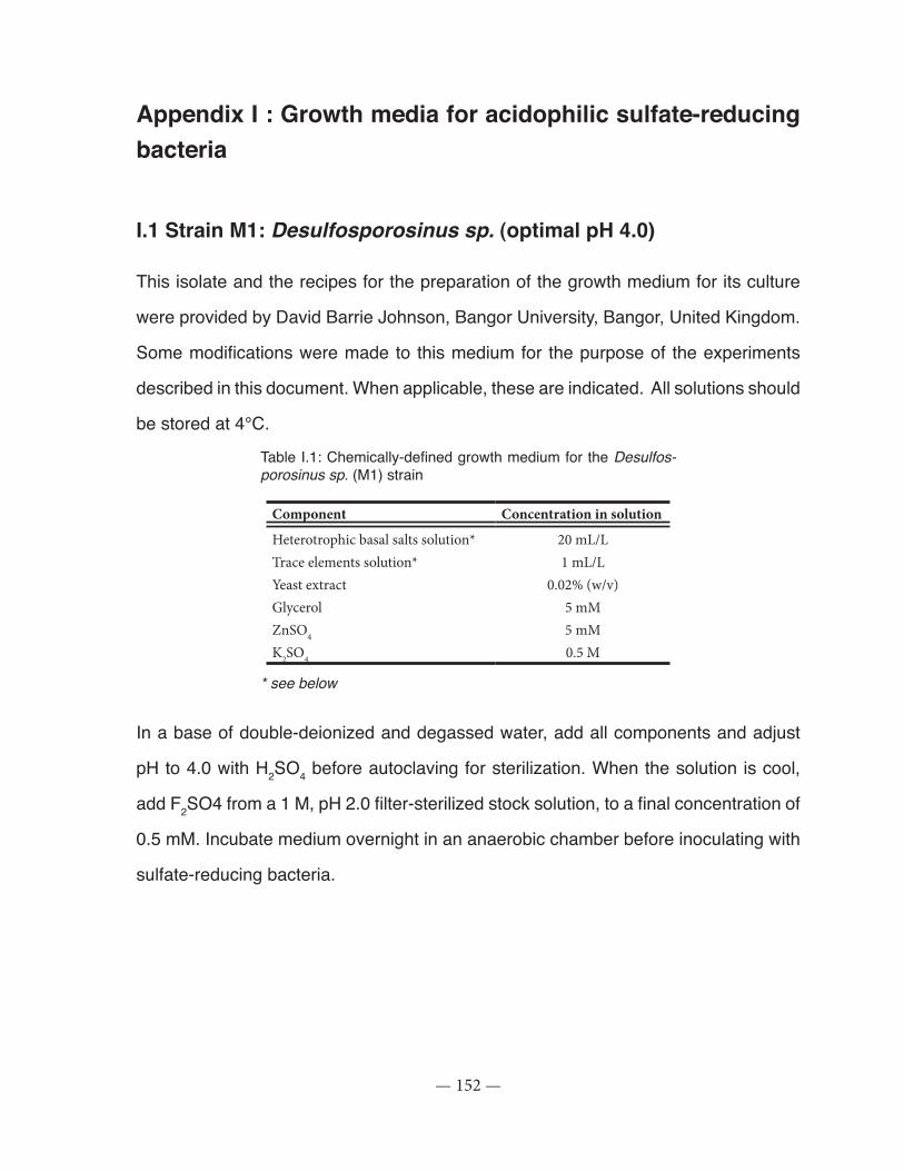
— 152 —
Appendix I : Growth media for acidophilic sulfate-reducing bacteria
I.1 Strain M1: Desulfosporosinus sp. (optimal pH 4.0)
This isolate and the recipes for the preparation of the growth medium for its culture
were provided by David Barrie Johnson, Bangor University, Bangor, United Kingdom.
Some modifications were made to this medium for the purpose of the experiments
described in this document. When applicable, these are indicated. All solutions should
be stored at 4°C.
Table I.1: Chemically-defined growth medium for the Desulfos-porosinus sp. (M1) strain
Component Concentration in solution
Heterotrophic basal salts solution* 20 mL/LTrace elements solution* 1 mL/LYeast extract 0.02% (w/v)Glycerol 5 mMZnSO4 5 mMK2SO4 0.5 M
* see below
In a base of double-deionized and degassed water, add all components and adjust
pH to 4.0 with H2SO4 before autoclaving for sterilization. When the solution is cool,
add F2SO4 from a 1 M, pH 2.0 filter-sterilized stock solution, to a final concentration of
0.5 mM. Incubate medium overnight in an anaerobic chamber before inoculating with
sulfate-reducing bacteria.
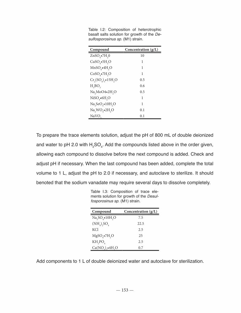
— 153 —
Table I.2: Composition of heterotrophic basalt salts solution for growth of the De-sulfosporosinus sp. (M1) strain.
Compound Concentration (g/L) ZnSO4•7H20 10CuSO4•5H2O 1MnSO4•4H2O 1CoSO4•7H2O 1Cr2(SO4)3•15H2O 0.5H3BO3 0.6Na2MoO4•2H2O 0.5NiSO4•6H2O 1Na2SeO4•10H2O 1Na2WO4•2H2O 0.1NaVO3 0.1
To prepare the trace elements solution, adjust the pH of 800 mL of double deionized
and water to pH 2.0 with H2SO4. Add the compounds listed above in the order given,
allowing each compound to dissolve before the next compound is added. Check and
adjust pH if necessary. When the last compound has been added, complete the total
volume to 1 L, adjust the pH to 2.0 if necessary, and autoclave to sterilize. It should
benoted that the sodium vanadate may require several days to dissolve completely.
Table I.3: Composition of trace ele-ments solution for growth of the Desul-fosporosinus sp. (M1) strain.
Compound Concentration (g/L)Na2SO4•10H2O 7.5(NH4)2SO4 22.5KCl 2.5MgSO4•7H2O 25KH2PO4 2.5Ca(NO3)2•4H2O 0.7
Add components to 1 L of double deionized water and autoclave for sterilization.
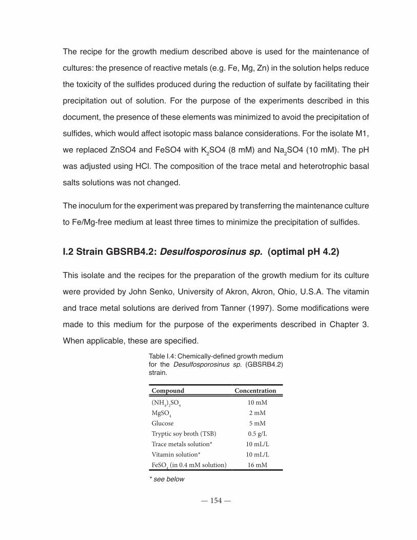
— 154 —
The recipe for the growth medium described above is used for the maintenance of
cultures: the presence of reactive metals (e.g. Fe, Mg, Zn) in the solution helps reduce
the toxicity of the sulfides produced during the reduction of sulfate by facilitating their
precipitation out of solution. For the purpose of the experiments described in this
document, the presence of these elements was minimized to avoid the precipitation of
sulfides, which would affect isotopic mass balance considerations. For the isolate M1,
we replaced ZnSO4 and FeSO4 with K2SO4 (8 mM) and Na2SO4 (10 mM). The pH
was adjusted using HCl. The composition of the trace metal and heterotrophic basal
salts solutions was not changed.
The inoculum for the experiment was prepared by transferring the maintenance culture
to Fe/Mg-free medium at least three times to minimize the precipitation of sulfides.
I.2 Strain GBSRB4.2: Desulfosporosinus sp. (optimal pH 4.2)
This isolate and the recipes for the preparation of the growth medium for its culture
were provided by John Senko, University of Akron, Akron, Ohio, U.S.A. The vitamin
and trace metal solutions are derived from Tanner (1997). Some modifications were
made to this medium for the purpose of the experiments described in Chapter 3.
When applicable, these are specified.
Table I.4: Chemically-defined growth medium for the Desulfosporosinus sp. (GBSRB4.2) strain.
Compound Concentration
(NH4)2SO4 10 mMMgSO4 2 mMGlucose 5 mMTryptic soy broth (TSB) 0.5 g/LTrace metals solution* 10 mL/LVitamin solution* 10 mL/LFeSO4 (in 0.4 mM solution) 16 mM
* see below

— 155 —
This medium was prepared by adding, in the anaerobic chamber (N2 95%, H2 5%)
each component of the growth medium to the prescribed concentration to degassed
double deionized water. Once the pH was adjusted, the medium was dispensed into
the appropriate container (serum tubes or vials for maintenance culture, large pyrex
bottles for experimental cultures) and these were sealed and taken out of the anaero-
bic chamber for autoclaving. The inoculum for the experiment was prepared by trans-
ferring the maintenance culture to Fe/Mg-free medium at least three times to minimize
the precipitation of sulfides from solution.
Table I.5: Composition of the trace metal solution for the strain Desulfosporosinus sp. (GBSRB4.2)
Component Concentration (g/L)
Nitrilotriacetic acid (from trisodium salt) 2.0MnSO4•H2O 1.0Fe(NH4)2(SO4)2•6H2O 0.8CoCL2•6H2O 0.2ZNSO4•7H2O 0.2CuCl2•2H2O 0.02NiCl2•6H2O 0.02Na2MoO4•2H2O 0.02Na2SeO4 0.02Na2WO4 0.02
The trace metal solution was prepared by adding each component in the prescribed
concentration to one liter of double-deionized water. The solution was not autoclaved.
Table I.6: Composition of the vitamin solution for the strain Desulfosporosinus sp. (GBSRB4.2)
Component Concentration (g/L)
Pyridoxine•HCl 10
Thiamine•HCl 5Riboflavin 5Calcium pantothenate 5Thioctic acid 5ρ-Aminobenzoic acid 5Nicotinic acid 5Vitamin B12 5
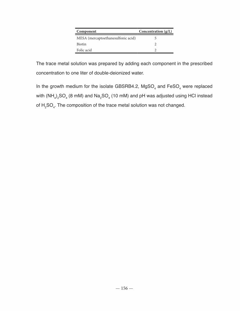
— 156 —
Component Concentration (g/L)
MESA (mercaptoethanesulfonic acid) 5Biotin 2Folic acid 2
The trace metal solution was prepared by adding each component in the prescribed
concentration to one liter of double-deionized water.
In the growth medium for the isolate GBSRB4.2, MgSO4 and FeSO4 were replaced
with (NH4)2SO4 (8 mM) and Na2SO4 (10 mM) and pH was adjusted using HCl instead
of H2SO4. The composition of the trace metal solution was not changed.
— 157 —
Appendix II: Sulfur reduction line
A significant portion of the PhD candidate’s time was spent building a sulfur extraction
line at the University of Ottawa, in the Earth Sciences Department (geobiology lab,
Dr. Fortin). The design of this extraction line was based on a similar installation at
McGill University, in the Earth and Planetary Sciences Department (Dr. Wing). Some
improvements and modifications were made to this design by the candidate, namely
to minimize the need to rely on complex glass parts that are expensive to make, fra-
gile, and require the work of a professional glassblower, as well as to take advantage
of the equipment already available at the University of Ottawa. This extraction line will
be dismantled and moved to the G.G. Hatch Stable Isotope Lab facilities at the Uni-
versity of Ottawa. Included in this appendix are a description of this installation and of
the parts used to build it.
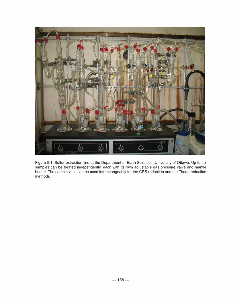
— 158 —
Figure II.1: Sulfur extraction line at the Department of Earth Sciences, University of Ottawa. Up to six samples can be treated independently, each with its own adjustable gas pressure valve and mantle heater. The sample vials can be used interchangeably for the CRS reduction and the Thode reduction methods.
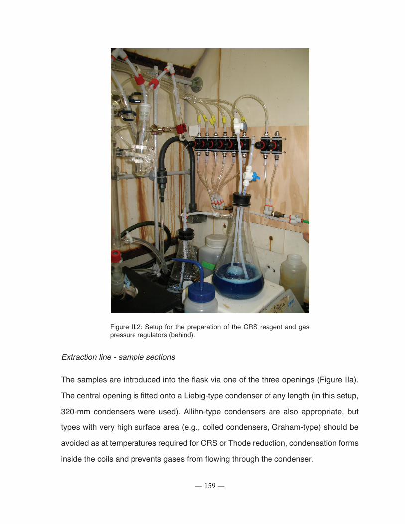
— 159 —
Figure II.2: Setup for the preparation of the CRS reagent and gas pressure regulators (behind).
Extraction line - sample sections
The samples are introduced into the flask via one of the three openings (Figure IIa).
The central opening is fitted onto a Liebig-type condenser of any length (in this setup,
320-mm condensers were used). Allihn-type condensers are also appropriate, but
types with very high surface area (e.g., coiled condensers, Graham-type) should be
avoided as at temperatures required for CRS or Thode reduction, condensation forms
inside the coils and prevents gases from flowing through the condenser.
— 160 —
A second flask opening is fitted with a 24/40 joint with GL-14 screw threading. As I was
unable to find a manufacturer producing standard 24/40 joints fitted with GL-14 threa-
ding, I had a glassblower affix the new threading to existing thermometer adapters
with a 24/40 joint. A glass rod connected to the gas inflow is passed through this GL-
14 cap, which is fitted with a sillicone ring liner. For the extraction of Thode-reducible
sulfates, the third and last opening is simply closed using a glass stopper, while for the
extraction of chromium-reducible sulfides, it is fitted with a 24/40 male joint with GL-14
threading fitted with a septum. The sample can be introduced through the septa once
the flask has been flushed with N2 gas to remove oxygen. The septa used in this par-
ticular installation are Labco Ltd. septa for Exetainer caps and can be pierced several
times before requiring replacement.
The top opening of the condensers are fitted with a 24/40 joint with GL-14 threading
fitted with a GL-14 cap and silicone ring. Teflon tubing is inserted into this opening and
connected to a single opening 24/40 vial via a push-to-connect 90° tube fitting cou-
pling attached to a 24/40 joint with double GL-14 threading inserted into a cylindrical
flask. The second opening of this joint features a GL-14 cap with silicone ring, into
which a section of teflon tubing is inserted. This teflon tubing is then inserted into the
sample vial.
Cold water is circulated via polypropylene tubing through all six condensers connec-
ted in series. All other tubing used in the extraction line is composed of teflon to mini-
mize reaction of organic compounds and the “sticking” of H2S to the lines. The 6-place
heating mantle used features 6 individual temperature controllers.
CRS reagent setup
An Erlenmeyer flask is positioned onto a stir plate and fitted with a rubber or silicone
stopper that has been pierced with two holes smaller than the diameter of the teflon
tubing (this has to be air tight to avoid reoxidation of the chemicals). Teflon tubing is
— 161 —
inserted into each hole and each section is fitted with a valve. One valve controls ac-
cess to the chemical with a syring and luer lock adapter, the other is connected to the
gas panel controller for N2 intake. The side outlet on the Erlenmeyer flask is connec-
ted to a section of polypropylene tubing that enters a 90° coupler directed into another
The CRS reagent (Figure II.2) can be removed from the flask through a 1/4 inch teflon
tube fitted with a female luer lock adapter.
Gas panel controller
The gas panel controller consists in a series of needle-valves and manifolds fixed to
a wooden plate inside the fume hood. A main line connected to a N2 tank enters the
panel from the right side (front of the fume hood, Figure II.2) and is split into two lines:
one line is used for the two needle valves on the right side of the panel (one for the
CRS reagent preparation and a spare valve) and the other split further into six for the
six sample lines in the extraction line. Each valve can be controlled separately and
with great precision.
Table II.1: List of parts used in the sulfur extraction line
Component Supplier Part numberExtraction line and reagent preparation3-neck round bottom flask, 24/40 joints, 250 mL Chemglass Inc. CG-1524Liebig condenser, 24/40 joint, 320 mm Chemglass Inc. CG-1218-01GL-14 cap with aperture Chemglass Inc. CGB-195-0124/40 joint Chemglass Inc.GL-14 Screw Thread Tube, on 12mm OD x 1.5mm W tubing, 100mm OAL
Chemglass Inc. CGB-194-01
Silicone Sealing Ring, fits GL-14 Cap, fits tubing O.D. 5.5mm to 6.5mm
Chemglass Inc. CGB-197-01
Teflon liners - long - for 24/40 standard taper jointa Chemglass Inc. CG-116-15Teflon liners - medium - for 24/25 standard taper jointa Chemglass Inc. CG-116-06Adapter, Thermometer, Inlet, 24/40 Inner Joint, 80mm Height, #7, Chemglass Inc.
Chemglass Inc. CG-1042-01
Extreme-Temperature Tubing Made with Teflon® PTFE (1/4» OD- outside diameter)
McMaster-Carr 5033K31
Polypropylene female luer lock - 1/8 McMaster-Carr 51525K293Septa for Labco Exetainer® 16.5mm Screw Caps Labco Ltd. VW101
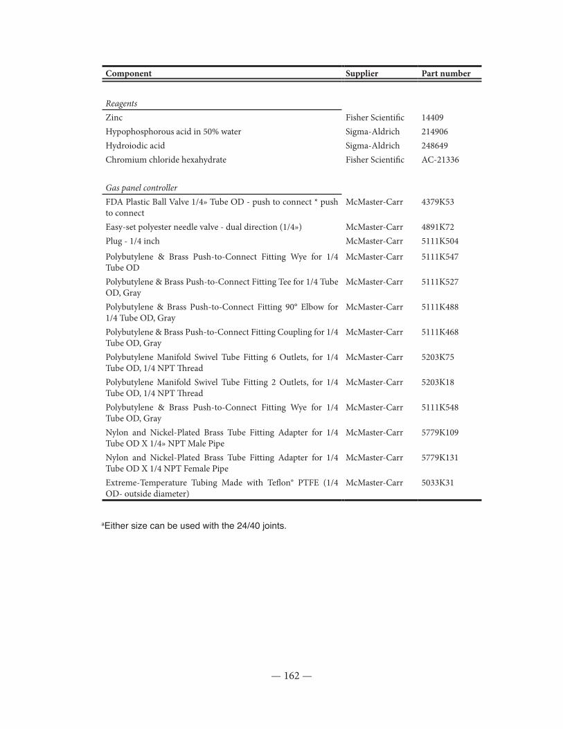
— 162 —
Component Supplier Part number
ReagentsZinc Fisher Scientific 14409 Hypophosphorous acid in 50% water Sigma-Aldrich 214906Hydroiodic acid Sigma-Aldrich 248649Chromium chloride hexahydrate Fisher Scientific AC-21336
Gas panel controllerFDA Plastic Ball Valve 1/4» Tube OD - push to connect * push to connect
McMaster-Carr 4379K53
Easy-set polyester needle valve - dual direction (1/4») McMaster-Carr 4891K72Plug - 1/4 inch McMaster-Carr 5111K504
Polybutylene & Brass Push-to-Connect Fitting Wye for 1/4 Tube OD
McMaster-Carr 5111K547
Polybutylene & Brass Push-to-Connect Fitting Tee for 1/4 Tube OD, Gray
McMaster-Carr 5111K527
Polybutylene & Brass Push-to-Connect Fitting 90° Elbow for 1/4 Tube OD, Gray
McMaster-Carr 5111K488
Polybutylene & Brass Push-to-Connect Fitting Coupling for 1/4 Tube OD, Gray
McMaster-Carr 5111K468
Polybutylene Manifold Swivel Tube Fitting 6 Outlets, for 1/4 Tube OD, 1/4 NPT Thread
McMaster-Carr 5203K75
Polybutylene Manifold Swivel Tube Fitting 2 Outlets, for 1/4 Tube OD, 1/4 NPT Thread
McMaster-Carr 5203K18
Polybutylene & Brass Push-to-Connect Fitting Wye for 1/4 Tube OD, Gray
McMaster-Carr 5111K548
Nylon and Nickel-Plated Brass Tube Fitting Adapter for 1/4 Tube OD X 1/4» NPT Male Pipe
McMaster-Carr 5779K109
Nylon and Nickel-Plated Brass Tube Fitting Adapter for 1/4 Tube OD X 1/4 NPT Female Pipe
McMaster-Carr 5779K131
Extreme-Temperature Tubing Made with Teflon® PTFE (1/4 OD- outside diameter)
McMaster-Carr 5033K31
aEither size can be used with the 24/40 joints.