Track and Vertex Reconstruction:

From Classical to Adaptive Methods

Are Strandlie

Gjøvik University College

P.O. Box 191, N-2802 Gjøvik, Norway ∗

Rudolf Fruhwirth

Institute of High Energy Physics of the Austrian Academy of Sciences

Nikolsdorfer Gasse 18, A-1050 Wien, Austria†

(Dated: October 9, 2009)

1

Abstract

The paper reviews classical and adaptive methods of track and vertex reconstruction

in particle physics experiments. Adaptive methods have been developed to meet

the experimental challenges at high-energy colliders, in particular the Large Hadron

Collider. They can be characterized by the obliteration of the traditional boundaries

between pattern recognition and statistical estimation, by the competition between

different hypotheses about what constitutes a track or a vertex, and by a high level

of flexibility and robustness achieved with a minimum of assumptions about the

data. The theoretical background of some of the adaptive methods is described,

and it is shown that there is a close connection between the two main branches of

adaptive methods: neural networks and deformable templates on the one hand, and

robust stochastic filters with annealing on the other hand. As both classical and

adaptive methods of track and vertex reconstruction presuppose precise knowledge

of the positions of the sensitive detector elements, the paper includes an overview

of detector alignment methods and a survey of the alignment strategies employed

by past and current experiments.

PACS numbers: 02.70.Rr,07.05.Kf,07.05.Mh,29.85.Fj

Keywords: Track finding, track fitting, vertex finding, vertex fitting, neural networks, Hopfield network, elastic

arms, deformable templates, deterministic annealing, Kalman filter, Gaussian-sum filter, EM algorithm, adaptive

filter, detector alignment

∗Also at Department of Physics, University of Oslo, Norway; Electronic address: Are.Strandlie@hig.no†Also at Department of Statistics and Probability Theory, University of Technology, Vienna, Austria; Elec-

tronic address: fru@hephy.oeaw.ac.at

2

Contents

I. Introduction 4

II. Classical methods of track and vertex reconstruction 6

A. Track finding 8

1. Conformal mapping 9

2. Hough and Legendre transform 9

3. Track road 10

4. Track following 10

B. Track fitting 11

1. Least-squares methods for track fitting 13

2. Removal of outliers and resolution of incompatibilities 16

3. Hybrid methods 17

C. Vertex finding 18

1. Cluster finding 19

2. Topological vertex finding 20

3. Minimum spanning tree 21

4. Feed-forward neural networks 22

D. Vertex fitting 22

1. Least-squares methods for vertex fitting 22

2. Robust vertex fitting 26

3. Vertex finding by iterated fitting 28

III. Adaptive methods 29

A. Hopfield neural networks 30

B. Elastic nets and deformable templates 33

C. Gaussian-sum filter 39

D. EM algorithm and adaptive track fitting 43

E. Comparative studies 46

F. Adaptive vertex fitting 50

IV. Detector alignment 53

3

A. Introduction 53

B. Global alignment 54

C. Iterative alignment 56

D. Experimental examples 57

1. Z factories 58

2. B factories 60

3. HERA 61

4. Hadron colliders 62

V. Conclusions 65

VI. Outlook 67

Acknowledgements 69

References 69

Figures 79

Tables 100

I. INTRODUCTION

Stupendous developments have taken place during the last decades in the fields of high-

energy physics accelerators, detectors and computing technologies. The desire to understand

in more detail the basic behaviour of the fundamental constituents of nature and the in-

teractions between these constituents has led to experimental studies carried out at ever

increasing energies. In general, the number of particles created by the interaction of two

particles rises with the collision energy. As a consequence, event patterns have become

much more complex in the course of time. In addition, data rates have increased in order

to enable the search for rare, interesting collision events immersed in a huge background of

events exhibiting well-known physics. Whereas most events in the experiments during the

1950s were studied manually on a scanning table, the data rate at the Large Hadron Collider

(LHC) at CERN, Geneva, Switzerland, has to be reduced online by more than five orders

of magnitude before the information from an event is written on mass storage for further

4

analysis. Tracking detectors have changed from bubble chambers to gaseous and solid-state

electronic detectors. Computers have changed from large mainframes to server farms with

processor speeds several orders of magnitude higher than those available some decades ago.

The task of analyzing data from high-energy physics experiments has therefore, over the

years, been performed in a continuously changing environment, and analysis methods have

evolved accordingly to adapt to these changes.

This paper aims to review methods employed in crucial parts of the data-analysis chain in

a high-energy physics experiment: the task of determining the basic kinematic parameters

of charged particles at their point of production, and the task of estimating the location of

these production points. These tasks are frequently called track reconstruction and vertex

reconstruction. Track and vertex reconstruction are done both online, especially in the high

level trigger, and offline. Online applications frequently use simplified methods, for the

sake of speed. The following discussion will concentrate on methods employed in the offline

analysis, where the ultimate precision is the major goal, and speed is rarely a decisive factor.

However, track and vertex reconstruction can attain their ultimate precision only if the

positions and orientations of the sensitive detector elements are known to high accuracy.

The review therefore includes detector alignment methods that are used for the precise de-

termination of the alignment constants (positions and orientations) of the sensitive detector

elements. In the experiments at the LHC the number of detector elements to be aligned runs

into several thousands, and in one case even exceeds ten thousand. Furthermore, the re-

quired precision is considerably higher than the intrinsic resolution of the detector elements

which in itself is already very small, on the order of ten micrometers. Detector alignment is

thus a highly non-trivial task that can ultimately only be solved by using information from

charged particles that cross several sensitive elements along their trajectory through the

detector. Alignment is therefore intimately connected to the track reconstruction challenge.

The topics of track and vertex reconstruction have over the years been reviewed several

times, with focus ranging from bubble chamber data-analysis methods (Jobes and Shaylor,

1972) through approaches applied in early electronic experiments (Eichinger and Regler,

1981; Grote, 1987) up to methods used in currently running experiments (Fruhwirth et al.,

2000; Mankel, 2004; Regler et al., 1996). In this review, however, we will put less emphasis

on traditional approaches but rather focus on more recently developed, adaptive methods

tailored to the needs of experiments of the LHC era. We will also make an attempt to describe

5

the theoretical background of some of these adaptive methods and show how different classes

of algorithms are intimately connected to each other. The underlying theory of how charged

particles interact with matter, as well as the basic detection principles and basic detector

types are excellently described in textbooks (e.g. Amsler et al., 2008; Bock and Vasilescu,

1998; Leo, 1994) and will not be covered here.

In contrast to a traditional approach, a method can be regarded as adaptive if it incor-

porates competition between several hypotheses, such that the outcome of the competition

depends on the current observations. In addition, the possibility of making soft decisions

and of combining hypotheses according to their posterior weights are typical features of an

adaptive method. Some of the adaptive methods have a strong Bayesian flavour, reflected

for example in the presence of posterior probabilities or weights attached to the different

hypotheses. The numerical values of the weights in general change after the inclusion of ad-

ditional information from the data. Methods can also exhibit different degrees of adaptivity,

depending on the level of prior assumptions inherent to the actual approach. The hallmark

of a good adaptive method is that it achieves maximum flexibility and robustness with as

few assumptions about the data as possible.

The review starts out in section II with a description of classical methods of track and

vertex reconstruction, followed in section III by an overview of adaptive methods applied to

the same tasks. Detector alignment is addressed in section IV, and the conclusions are given

in section V. An outlook to future research containing the authors’ opinions about the most

important unsolved problems in the topics described in this article is given in section VI.

II. CLASSICAL METHODS OF TRACK AND VERTEX RECONSTRUCTION

In any analysis of the data of a high-energy physics experiment, it is of crucial impor-

tance to estimate as accurately as possible the kinetic parameters of particles produced in a

collision event, e.g. the position, direction and momentum of the particles at their produc-

tion points. For this purpose, a set of detecting devices providing high-precision position

measurements are positioned close to the beam collision area. Charged particles created

in the collisions ionize the material of detecting devices on their way out of the collision

area, providing several position measurements along the trajectory of each particle. The

detector elements should disturb the trajectory of the particles as little as possible. Hence,

6

the amount of material present in such tracking detectors should be kept at a minimum.

The task of track reconstruction is traditionally divided into two different subtasks: track

finding and track fitting. Track finding is a pattern recognition or classification problem and

aims at dividing the set of measurements in a tracking detector into subsets, each subset

containing measurements believed to originate from the same particle. These subsets are

called track candidates. An additional subset contains measurements believed not to come

from any of the interesting tracks, but for instance from noise in the electronics or from low-

energy particles spiraling inside the tracking detector. Track finding should be conservative

and keep a track candidate in case of doubt rather than discarding it, as a track candidate

discarded at this stage is impossible to recover at any later stage. An example of a hard

track finding problem is shown in Fig. 1. It is the task of the track finding to reconstruct

the correct classification of the hits, shown in the bottom panel, to their respective tracks,

shown in the top panel.

The track fit takes the set of measurements in a track candidate as a starting point.

The goal is to estimate as accurately as possible a set of parameters describing the state

of the particle somewhere in the tracking detector, often at a reference surface close to the

particle beam. With very few exceptions (for example Chernov et al., 1993; James, 1983), the

estimation is based on least-squares methods. The track fit should be as computationally fast

as possible, it should be robust against mistakes made during the track finding procedure,

and it should be numerically stable.

The track fit is also used to decide whether the track candidate hypothesis is valid. Such

a test can be based on the value of the χ2 statistic, i.e. the sum of the squared standardized

differences between the measured positions in the track candidate and the estimated posi-

tions of the track at the points of intersection of the detector devices. If the value of such a

statistic is too high, the set of measurements is not statistically compatible with the hypoth-

esis of having been created by a single particle. The reason for this incompatibility could

be a single or a few measurements in a track candidate misclassified by the track finding,

or a track candidate being completely wrong in the sense that it is a random collection of

measurements originating from several other particles — so-called ghost tracks. The track

fit should in this testing phase be able to remove wrong or outlying measurements in the

track candidates and suppress the ghost tracks completely.

The step following track reconstruction is vertex reconstruction. A vertex is a point where

7

particles are produced, either by a collision of a beam particle with another beam particle

or a target particle, or by the decay of a particle, or by an interaction of a particle with the

material of the detector. Vertex reconstruction offers the following benefits:

• Using the vertex constraint, the momentum estimates of the particles involved can be

improved.

• A neutral or very short-lived particle can be reconstructed by finding its decay products

and fitting them to a common vertex.

• The decay length of a short-lived particle can be determined by computing the distance

between its estimated production vertex and its estimated decay vertex.

Similar to track reconstruction, the task of vertex reconstruction can be divided into

vertex finding and vertex fitting. The starting point of vertex finding is the set of all valid

tracks provided by the track reconstruction, represented by a list of track parameter vectors.

The vertex finding algorithms classifies the tracks into vertex candidates, which are fed into

the vertex fit. The output of the vertex fit is a list of vertices, each entry containing the

estimated vertex position as well as a set of updated track parameter vectors of the particles

associated to that particular production point. Again the χ2 or a related statistic can be

used to test the vertex hypothesis.

A. Track finding

In experimental conditions such as those found in the LHC experiments, many of the

measurements are either noise or belonging to particles with too low energy to be interesting

from a physics point of view. Therefore, many hypotheses have to be explored in order to

find the set of interesting track candidates, and track finding can in general be a cumbersome

and time-consuming procedure. Computational speed is an important issue, and the choice

of algorithms may be dictated by this fact. Track finding often uses the knowledge of how

a charged particle moves inside the bulk of the detector, the so-called track model, but can

resort to a simplified version if time consumption is critical. The use of simplified track

models is particularly important for triggering applications, where track finding is part of

the strategy applied in the online selection procedure of interesting events. Such applications

8

are not considered in this paper, which will concentrate on methods used for offline analysis

of data, i.e. analysis of data available on mass storage.

Methods of track finding can in general be classified as global or local. Global meth-

ods treat all measurements simultaneously, whereas local methods go through the list of

measurements sequentially. Examples of global approaches presented below are conformal

mapping, Hough transform, and Legendre transform, whereas the track road and track

following methods are regarded as local.

1. Conformal mapping

The conformal mapping method (Hansroul et al., 1988) for track finding is based on the

fact that circles going through the origin of a two-dimensional x–y coordinate system maps

onto straight lines in a u–v coordinate system by the transformation

u =x

x2 + y2, v =

y

x2 + y2, (1)

where the circles are defined by the circle equation (x− a)2 + (y − b)2 = r2 = a2 + b2. The

straight lines in the u–v plane are then given by

v =1

2b− ua

b. (2)

For large values of r or, equivalently, high-momentum tracks, the straight lines are passing

close to the origin, and track candidates can be obtained by transforming the measurements

in the u–v plane to azimuthal coordinates and collecting the angular part of the measure-

ments in a histogram. Track candidates are found by searching for peaks in this histogram.

2. Hough and Legendre transform

In the case of straight lines not necessarily passing close to the origin, i.e. for tracks in

a larger range of momenta, a more general approach is needed in order to locate the lines.

The Hough transform (Hough, 1959) is well suited for such a task. The idea is based on

a simple transformation of the equation of a straight line in an x–y plane, y = cx + d, to

another straight line in a c–d plane, d = −xc + y. The points along the line in the c–d

plane correspond to all possible lines going through the point (x, y) in the x–y plane. Points

9

lying along a straight line in the x–y plane therefore tend to create lines in the c–d plane

crossing at the point which specifies the actual parameters of that line in the x–y plane.

In practice, the c–d space is often discretized, allowing a set of bins to be incremented

for each of the measurements in the x–y space. As for the conformal mapping method,

the position of peaks in the histogram provides information about the parameters of the

lines in the x–y space. In contrast to the one-dimensional parameter space of the conformal

mapping method, the parameter space is in this case two-dimensional. The Hough transform

rapidly loses efficiency for finding tracks if one attempts to move to a parameter space with

a dimension higher than two.

For track finding in drift tubes, the drift circles provided by the knowledge of the drift

distances of each of the measurements can be transformed to sine curves in the azimuthal

coordinate system by applying a Legendre transform (Alexopoulos et al., 2008). Peaks at

the intersections of several sine curves in this coordinate system give not only the set of drift

tubes hit by the same particle, but also the solution to the left-right ambiguity problem

inherent to this kind of detector system. An illustration is shown in Fig. 2.

3. Track road

An example of a local approach to track finding is the so-called track road method. It

is initiated with a set of measurements that could have been created by the same charged

particle. The track model, i.e. the shape of the trajectory, can be used to interpolate

between the measurements and create a road around the trajectory. Measurements inside

the boundaries of the road constitute the track candidate. The number of measurements

and the quality of the subsequent track fit are used to evaluate the correctness of the track

hypothesis.

4. Track following

A related approach is track following, which starts from a track seed. Most of the times,

the seed is a short track segment built from a few measurements. In addition it can be

constrained to point to the interaction region. Seeds can be constructed in the inner region

of the tracking detector close to the interaction region, where the measurements frequently

10

are of very high precision, or in the outer region, where the track density is lower. From the

seed, the track is extrapolated to the next detector layer containing a measurement. The

measurement closest to the predicted track is included in the track candidate. This procedure

is iterated until too many detector layers with missing measurements are encountered or until

the end of the detector system is reached.

B. Track fitting

The track fit aims at estimating a set or vector of parameters representing the kine-

matic state of a charged particle from the information contained in the various position

measurements in the track candidate. Since these positions are stochastic quantities with

uncertainties attached to them, the estimation amounts to some kind of statistical proce-

dure. In addition to estimated values of the track parameters, the track fit also provides

a measure of the uncertainty of these values in terms of the covariance matrix of the track

parameter vector.

Most estimation methods can be decomposed into a set of basic building blocks, and the

methods differ in the logic of how these blocks are combined.

a. Track parametrization. If tied to a surface, five parameters are sufficient to uniquely de-

scribe the state of a charged particle. The actual choice of track parameters depends on

e.g. the geometry of the tracking detector. In a detector consisting of cylindrical detector

layers, the reference surface is often cylindrical and makes the radius times the azimuthal

angle (RΦ) the natural choice of one of the position parameters. In a detector consist-

ing of planar detector layers, however, Cartesian position coordinates are more frequently

used (Fruhwirth et al., 2000).

b. Track model. The track model describes how the track parameter or state vector at a

given surface k depends on the state vector on a different surface i:

qk = fk|i(qi), (3)

where fk|i is the track propagator from surface i to surface k and q is the state vector.

An illustration is found in Fig. 3. For simple surfaces, the track model is analytical in

11

a vanishing magnetic field (straight line) or in a homogeneous field (helix). If the field is

inhomogeneous, one has to resort to numerical schemes such as Runge-Kutta integration of

the equation of motion.

c. Error propagation. During the track parameter estimation procedure, propagation of the

track parameter covariance matrix along with the track parameters themselves is often

requested. The standard procedure for this so-called linear error propagation is a similarity

transformation between layers i and k,

Ck = Fk|iCiFk|iT, (4)

where C is the covariance matrix and Fk|i is the Jacobian matrix of the propagation from

layer i to k,

Fk|i =∂qk∂qi

. (5)

For analytical track models the Jacobian is also analytical (Strandlie and Wittek, 2006).

In inhomogeneous magnetic fields, the derivatives can be calculated by purely numerical

schemes or by semi-analytical propagation of the derivatives in parallel to the Runge-Kutta

propagation of the track parameters (Bugge and Myrheim, 1981).

d. Material effects. The most important effects on the trajectory of charged particles caused

by material present in the detector volume are ionization energy loss and multiple Coulomb

scattering (Amsler et al., 2008). For light particles such as electrons, radiation energy loss by

bremsstrahlung also plays an important role. The fluctuations of ionization energy loss are

usually quite small, and such energy loss is therefore normally treated during track fitting

as a deterministic correction to the state vector (Fruhwirth et al., 2000). Bremsstrahlung

energy loss, on the other hand, suffers from large fluctuations (Bethe and Heitler, 1934)

and affects therefore both the state vector and its covariance matrix. Multiple Coulomb

scattering is an elastic process, which in a thin scatterer disturbs only the direction of

a passing charged particle; in a sufficiently thick scatterer, also the position in a plane

transversal to the incident direction is changed (Amsler et al., 2008). Since the mean value

of the scattering angle and an eventual offset is zero, only the covariance matrix is updated

in order to incorporate the effects of multiple scattering into the track fitting procedure.

12

e. Measurement model. The measurement model hk describes the functional dependence of

the measured quantities in layer k, mk, on the state vector at the same layer,

mk = hk(qk). (6)

The vector of measurements mk usually consists of the measured positions but can also

contain other quantities, e.g. measurements of direction or even momentum. During the

estimation procedure the Jacobian Hk of this transformation is often needed,

Hk =∂mk

∂qk. (7)

In many cases the Jacobian contains only rotations and projections and can thus be com-

puted analytically.

1. Least-squares methods for track fitting

The overwhelming majority of experimental implementations use some kind of linear

least-squares approach for the task of track fitting. The linear, global least-squares method

is optimal if the track model is linear, i.e. if the track propagator fk|i from detector layer

i to detector layer k is a linear function of the state vector qi, and if all probability densi-

ties encountered during the estimation procedure are Gaussian. If the track propagator is

non-linear, the linear least-squares method is still the optimal linear estimator. However,

although least-squares estimators are easy to compute, they lack robustness (Rousseeuw and

Leroy, 1987).

The starting point for deriving the global least-squares method is the functional relation-

ship between the initial state q0 of the particle at the reference surface and the vector of

measurements mk at detector layer k,

mk = dk(q0) + γk, (8)

where dk is a composition of the measurement model function mk = hk(qk) and the track

propagator functions:

dk = hk fk|k−1 · · · f2|1 f1|0. (9)

The term γk is stochastic and contains all multiple Coulomb scattering up to layer k as well

as the measurement error of mk. A linear estimator requires a linearized track model, and

13

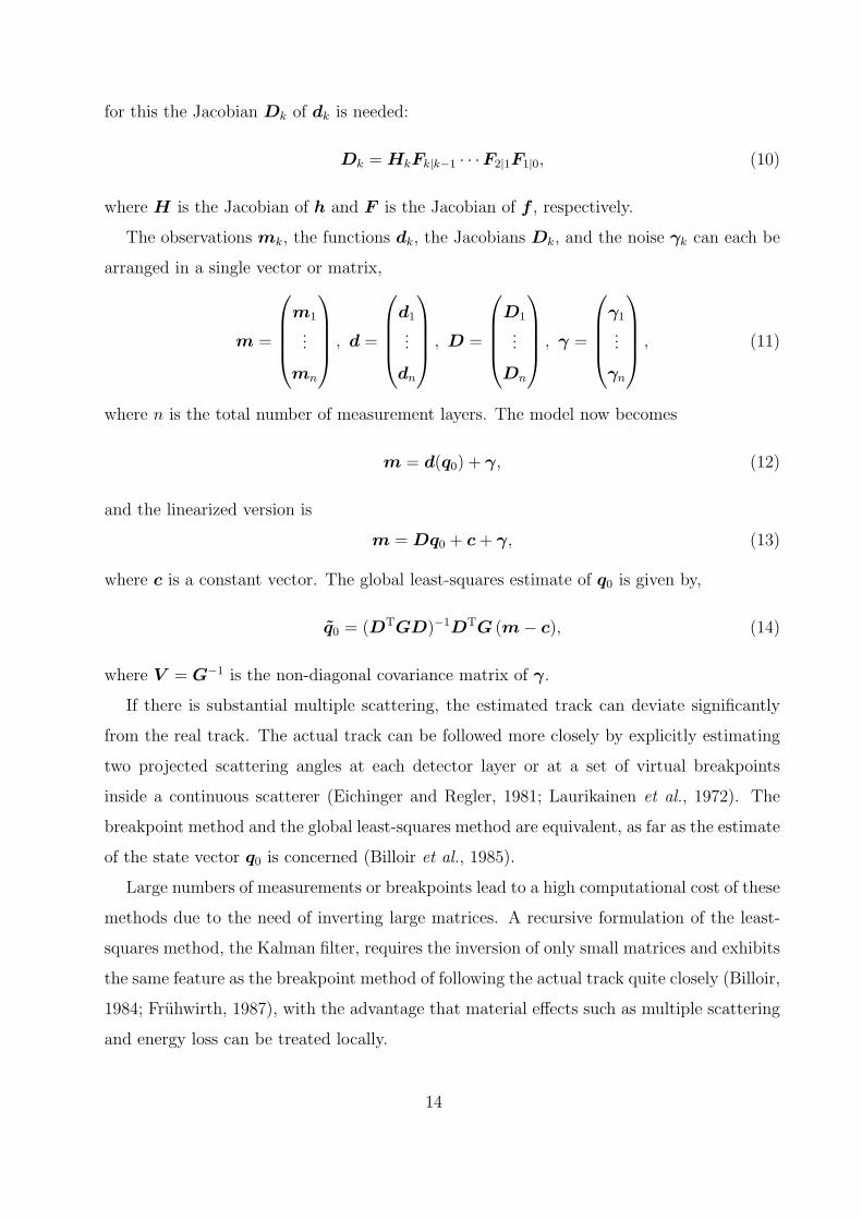
for this the Jacobian Dk of dk is needed:

Dk = HkFk|k−1 · · ·F2|1F1|0, (10)

where H is the Jacobian of h and F is the Jacobian of f , respectively.

The observations mk, the functions dk, the Jacobians Dk, and the noise γk can each be

arranged in a single vector or matrix,

m =

m1

...

mn

, d =

d1

...

dn

, D =

D1

...

Dn

, γ =

γ1

...

γn

, (11)

where n is the total number of measurement layers. The model now becomes

m = d(q0) + γ, (12)

and the linearized version is

m = Dq0 + c+ γ, (13)

where c is a constant vector. The global least-squares estimate of q0 is given by,

q0 = (DTGD)−1DTG (m− c), (14)

where V = G−1 is the non-diagonal covariance matrix of γ.

If there is substantial multiple scattering, the estimated track can deviate significantly

from the real track. The actual track can be followed more closely by explicitly estimating

two projected scattering angles at each detector layer or at a set of virtual breakpoints

inside a continuous scatterer (Eichinger and Regler, 1981; Laurikainen et al., 1972). The

breakpoint method and the global least-squares method are equivalent, as far as the estimate

of the state vector q0 is concerned (Billoir et al., 1985).

Large numbers of measurements or breakpoints lead to a high computational cost of these

methods due to the need of inverting large matrices. A recursive formulation of the least-

squares method, the Kalman filter, requires the inversion of only small matrices and exhibits

the same feature as the breakpoint method of following the actual track quite closely (Billoir,

1984; Fruhwirth, 1987), with the advantage that material effects such as multiple scattering

and energy loss can be treated locally.

14

The Kalman filter proceeds by alternating prediction and update steps (see Fig. 4). The

prediction step propagates the estimated track parameter qk−1|k−1 vector from detector layer

k − 1 to the next layer containing a measurement:

qk|k−1 = fk|k−1(qk−1|k−1), (15)

as well as the associated covariance matrix

Ck|k−1 = Fk|k−1Ck−1|k−1Fk|k−1T +Qk, (16)

where Qk is the covariance matrix of multiple scattering after layer k−1 up to and including

layer k. The part of Qk arising from scattering between the layers has to be propagated to

layer k by the appropriate Jacobian.

The update step corrects the predicted state vector by using the information from the

measurement in layer k:

qk|k = qk|k−1 +Kk

[mk − hk(qk|k−1)

], (17)

where the gain matrix Kk is given by:

Kk = Ck|k−1HkT(Vk +HkCk|k−1Hk

T)−1

, (18)

and Vk is the covariance matrix of mk. The covariance matrix is updated by:

Ck|k = (I −KkHk)Ck|k−1. (19)

An alternative formulation of the Kalman filter operates on the inverse covariance ma-

trices (weight or information matrices) rather than on the covariance matrices them-

selves (Fruhwirth, 1987). This approach tends to be numerically more stable than the

gain matrix formulation.

The full information at the end of the track as provided by the filter can be propagated

back to all previous estimates by another iterative procedure, the Kalman smoother. A step

of the smoother from layer k + 1 to layer k is for the state vector:

qk|n = qk|k +Ak(qk+1|n − qk+1|k), (20)

where the smoother gain matrix is given by:

Ak = Ck|kFk+1|kT(Ck+1|k)

−1. (21)

15

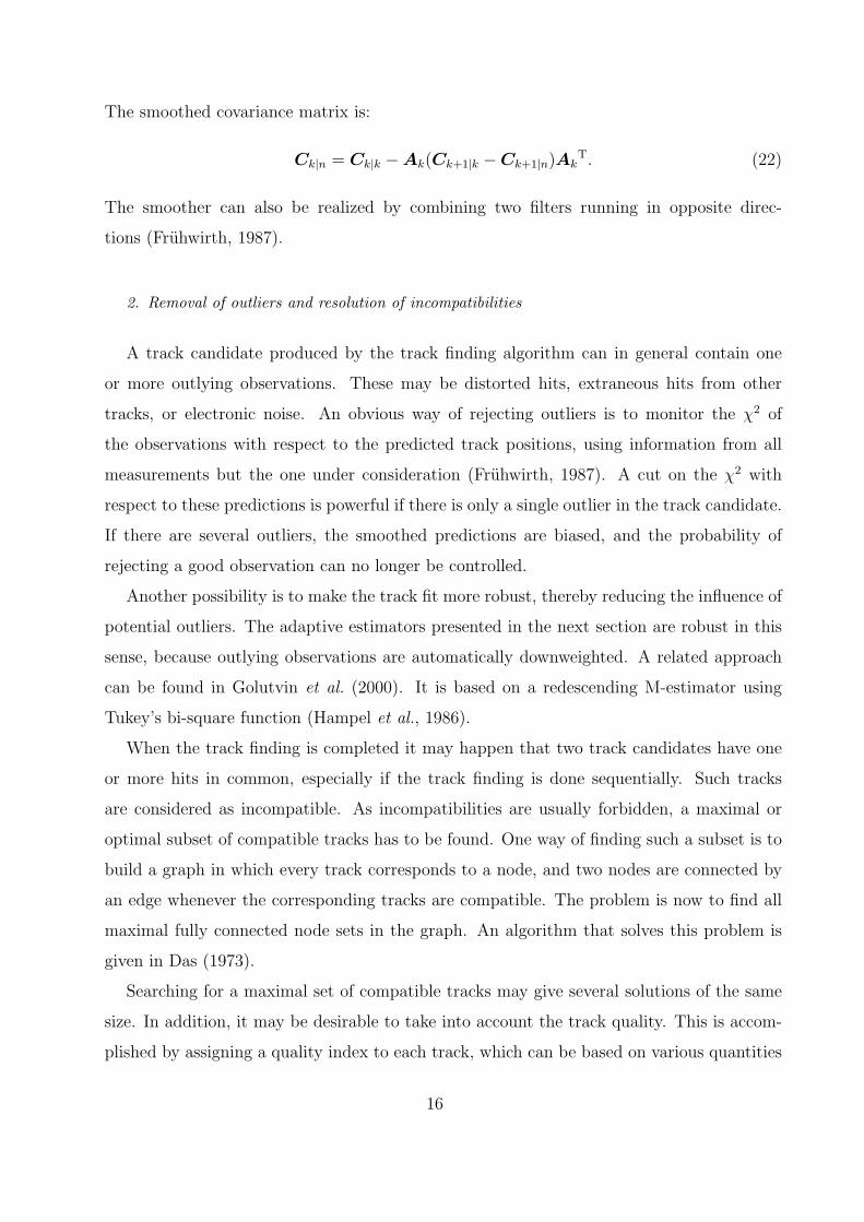
The smoothed covariance matrix is:

Ck|n = Ck|k −Ak(Ck+1|k −Ck+1|n)AkT. (22)

The smoother can also be realized by combining two filters running in opposite direc-

tions (Fruhwirth, 1987).

2. Removal of outliers and resolution of incompatibilities

A track candidate produced by the track finding algorithm can in general contain one

or more outlying observations. These may be distorted hits, extraneous hits from other

tracks, or electronic noise. An obvious way of rejecting outliers is to monitor the χ2 of

the observations with respect to the predicted track positions, using information from all

measurements but the one under consideration (Fruhwirth, 1987). A cut on the χ2 with

respect to these predictions is powerful if there is only a single outlier in the track candidate.

If there are several outliers, the smoothed predictions are biased, and the probability of

rejecting a good observation can no longer be controlled.

Another possibility is to make the track fit more robust, thereby reducing the influence of

potential outliers. The adaptive estimators presented in the next section are robust in this

sense, because outlying observations are automatically downweighted. A related approach

can be found in Golutvin et al. (2000). It is based on a redescending M-estimator using

Tukey’s bi-square function (Hampel et al., 1986).

When the track finding is completed it may happen that two track candidates have one

or more hits in common, especially if the track finding is done sequentially. Such tracks

are considered as incompatible. As incompatibilities are usually forbidden, a maximal or

optimal subset of compatible tracks has to be found. One way of finding such a subset is to

build a graph in which every track corresponds to a node, and two nodes are connected by

an edge whenever the corresponding tracks are compatible. The problem is now to find all

maximal fully connected node sets in the graph. An algorithm that solves this problem is

given in Das (1973).

Searching for a maximal set of compatible tracks may give several solutions of the same

size. In addition, it may be desirable to take into account the track quality. This is accom-

plished by assigning a quality index to each track, which can be based on various quantities

16

such as the χ2 statistic, the track length, the distance of the track from the interaction re-

gion, the direction of the track, et cetera. The best maximal compatible node set is now the

one that maximizes the sum of all quality indices. Finding the best node set has been solved

by a recurrent neural network (Hopfield network, see III.A). The network and an application

to one of the forward chambers of the DELPHI experiment is described in Fruhwirth (1993).

Another algorithm, developed for the global solution of tracking ambiguities in DELPHI, is

described in Wicke (1998).

3. Hybrid methods

The Kalman filter can be used for track finding and track fitting concurrently (Billoir,

1989; Billoir and Qian, 1990). The resulting progressive track finding algorithm can be

regarded as an optimal track following procedure. The algorithm is illustrated in Fig. 5. It

starts out with finding seeds in a couple of adjacent layers, then follows each seed through

the detector and picks up compatible hits as it goes along. If not enough compatible hits

are found the candidate is dropped. In practice, some of the seeds can be discarded right

away because their momentum is too small or because they do not point to the interaction

point.

In the original formulation of this strategy, the χ2 of the residual of the measurement mk

with respect to the predicted state,

χ2k,+ = rk|k−1

TR−1k|k−1rk|k−1, (23)

with

rk|k−1 = mk − hk(qk|k−1), (24)

and the covariance matrix of the residual given by

Rk|k−1 = Vk +HkCk|k−1HT, (25)

is used to evaluate the statistical compatibility of the measurement with the prediction. If

there are several compatible measurements, the one with the lowest value of the χ2 statistic

is included in the track candidate and used for the update step of the Kalman filter.

If there are many nearby tracks or a high density of noisy measurements, the measurement

closest to the predicted track might not necessarily belong to the track under consideration.

17

In order to cope with such a situation, the procedure outlined above can be generalized to

a so-called combinatorial Kalman filter (CKF; Mankel, 1997). It marks the transition from

classical to adaptive methods insofar as several hypotheses about the track are entertained

simultaneously until in the end one of them is declared as the winner.

Like the progressive track finding, the CKF starts from a seed, usually a short track

segment at the inner or the outer end of a tracking detector. If there are several compatible

measurements in the first layer after the seed, several Kalman filter branches are generated,

each of them containing a unique, compatible measurement at the end of the branch. In

order to handle potential detector inefficiencies, a branch with a missing measurement is

also created. All branches are propagated to the next detector layer containing at least one

compatible measurement, and new branches are created for each combination of predicted

states compatible with a measurement. This procedure leads to a combinatorial tree of

Kalman filters running in parallel. Branches are removed if the total quality of the branch

— in terms of the total χ2 of the track candidate up to the layer under consideration — falls

below a defined value, or if too many consecutive layers without compatible measurements

are traversed. In the end, the surviving branch with the highest quality — usually in terms

of a combination of the total χ2 and the total number of measurements — is kept. An

example is shown in Fig. 6.

A similar track finding method has been formulated in the language of cellular au-

tomata (Glazov et al., 1993; Kisel, 2006; Kisel et al., 1997). The cellular automaton ap-

proach can on one hand be regarded as local, as it builds up branches using information

from measurements in nearby layers. On the other hand, the procedure is not initiated from

a seed. All measurements are processed in parallel, making the approach a hybrid between

a local and a global method.

C. Vertex finding

Vertex finding is the task of classifying the reconstructed tracks in an event into vertex

candidates such that all tracks associated with a candidate originate at that vertex. There

are several types of vertices, and different strategies may be required to find them.

• If the particles are produced by the collision of two beam particles (in a collider

experiment) or a beam particle and a target particle (in a fixed-target experiment),

18

the vertex is a primary vertex.

• If the particles are produced by the decay of an unstable particle, the vertex is a

secondary decay vertex. An example is the decay K0S −→ π+π−.

• If the particles are produced by the interaction of a particle with the material of the

detector, the vertex is a secondary interaction vertex. An example is bremsstrahlung,

the radiation of a photon by an electron in the electric field of a nucleus.

The primary vertex in an event is usually easy to find, especially if prior information

about its location is available, such as the beam profile or the target position. A notable

exception is the invisible primary vertex of a Υ(4S)→ B0B0 decay at a B factory. On the

other hand, secondary decay vertices of short-lived particles may be hard to find, as some of

the decay products may also be compatible with the primary vertex. An example is shown

in Fig. 7. In this example one of the primary tracks passes very close to the secondary vertex

(top panel). This could lead to a wrong assignment of this track. The bottom panel shows

that some of the secondary tracks, when extrapolated back into beam tube, pass very close

to the primary vertex. This could result in a wrong assignment of these tracks. In order to

achieve optimal separation of primary and secondary vertices, the spatial resolution of the

innermost layers and the minimization of the material is of the utmost importance.

1. Cluster finding

Clustering methods are based on a distance matrix or a similarity matrix of the objects

to be classified. A cluster is then a group with small distances (large similarities) inside the

group and large distances (small similarities) to objects outside the group. The distance

measure reflects only the geometry of the tracks. Hierarchical clustering builds a tree of

clusterings. Agglomerative methods start at the leaves of the tree, i.e. the single objects,

while divisive methods start at the root, the totality of all objects.

In the simplest case, the clustering can be reduced to a one-dimensional problem. An

example is primary vertex finding in the pixel detector of the CMS experiment at the

LHC (Cucciarelli, 2005). The input of the algorithm consists of triplets of pixel hits that

are compatible with a track hypothesis. From each triplet the longitudinal impact point zIP

and its error is computed. Clusters are found by two methods. With the histogramming

19

method, the impact points are filled into a histogram. Empty bins are discarded, and the

non-empty bins are scanned along z. A cluster is defined as a contiguous set of consecutive

bins separated by a distance smaller than a threshold ∆z. After a cleaning procedure, the z

positions of the clusters are recomputed as a weighted zIP average of the remaining tracks,

the weights being the inverse squared errors of the longitudinal impact points. The primary

vertex is identified as the cluster with the largest sum of squared transverse momenta.

The second method described in Cucciarelli (2005) is a hierarchical clustering of the

divisive kind. The tracks are ordered by increasing zIP, and the ordered list is scanned. A

cluster is terminated when the gap between two consecutive tracks exceeds a threshold, and

a new cluster is started. For each initial cluster, an iterative procedure is applied to discard

incompatible tracks. The discarded tracks are recovered to form a new cluster, and the same

procedure is applied again, until there are less than two remaining tracks.

In the general case, clustering proceeds in space. Various clustering methods have been

evaluated in the context of vertex finding, of both the hierarchical and the non-hierarchical

type (Waltenberger, 2004). In hierarchical, agglomerative clustering each track starts out

as a single cluster. Clusters are merged iteratively on the basis of a distance measure. The

shortest distance in space between two tracks is peculiar insofar as it does not satisfy the

triangle inequality: if tracks a and b are close, and tracks b and c are close, it does not

follow that tracks a and c are close as well. The distance between two clusters of tracks

should therefore be defined as the maximum of the individual pairwise distances, known

as complete linkage in the clustering literature. Divisive clustering starts out with a single

cluster containing all tracks. Further division of this cluster can be based on repeated vertex

estimation with identification of outliers. Some examples of the approach are described below

in subsection II.D.3.

2. Topological vertex finding

A very general topological vertex finder (ZVTOP) was proposed in Jackson (1997). It

is related to the Radon transform, which is a continuous version of the Hough transform

used for track finding (see II.A). The search for vertices is based on a function V (v) which

quantifies the probability of a vertex at location v. For each track a Gaussian probability

20

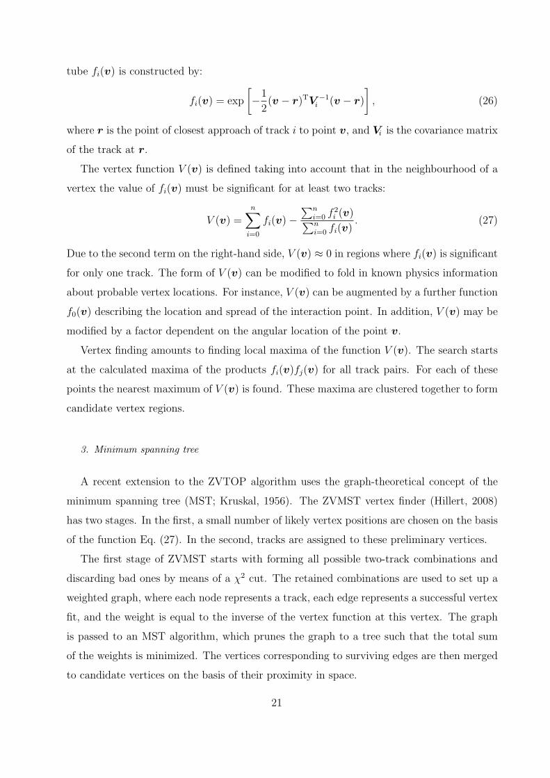
tube fi(v) is constructed by:

fi(v) = exp

[−1

2(v − r)TV −1

i (v − r)

], (26)

where r is the point of closest approach of track i to point v, and Vi is the covariance matrix

of the track at r.

The vertex function V (v) is defined taking into account that in the neighbourhood of a

vertex the value of fi(v) must be significant for at least two tracks:

V (v) =n∑

i=0

fi(v)−∑n

i=0 f2i (v)∑n

i=0 fi(v). (27)

Due to the second term on the right-hand side, V (v) ≈ 0 in regions where fi(v) is significant

for only one track. The form of V (v) can be modified to fold in known physics information

about probable vertex locations. For instance, V (v) can be augmented by a further function

f0(v) describing the location and spread of the interaction point. In addition, V (v) may be

modified by a factor dependent on the angular location of the point v.

Vertex finding amounts to finding local maxima of the function V (v). The search starts

at the calculated maxima of the products fi(v)fj(v) for all track pairs. For each of these

points the nearest maximum of V (v) is found. These maxima are clustered together to form

candidate vertex regions.

3. Minimum spanning tree

A recent extension to the ZVTOP algorithm uses the graph-theoretical concept of the

minimum spanning tree (MST; Kruskal, 1956). The ZVMST vertex finder (Hillert, 2008)

has two stages. In the first, a small number of likely vertex positions are chosen on the basis

of the function Eq. (27). In the second, tracks are assigned to these preliminary vertices.

The first stage of ZVMST starts with forming all possible two-track combinations and

discarding bad ones by means of a χ2 cut. The retained combinations are used to set up a

weighted graph, where each node represents a track, each edge represents a successful vertex

fit, and the weight is equal to the inverse of the vertex function at this vertex. The graph

is passed to an MST algorithm, which prunes the graph to a tree such that the total sum

of the weights is minimized. The vertices corresponding to surviving edges are then merged

to candidate vertices on the basis of their proximity in space.

21

In the second stage of ZVMST tracks are associated to the candidate vertices, based

both on values of the probability tubes (see Eq. (26)) and the values of the vertex functions

(see Eq. (27)) at the candidate positions.

4. Feed-forward neural networks

Feed-forward neural networks, also called multi-layer perceptrons, are classifiers that learn

their decision rules on a training set of data with known classification. If the data at hand

do not conform to the properties of the training sample, the network cannot cope with this

situation. Such networks therefore cannot be considered as adaptive.

Primary vertex finding with a feed-forward neural network was proposed in Lindsey and

Denby (1991). The input to the network was provided by the drift times of tracks in a

planar drift chamber parallel to the colliding proton–antiproton beams. The chamber was

divided into overlapping 18-wire subsections. The 18 wires correspond to the 18 input units

of the network. The hidden layer of the network had 128 neurons, and the output layer had

62 units, corresponding to 62 1-cm bins along the beam line (see Fig. 8). The network was

trained by back-propagation on 12000 patterns, a mixture of events with single tracks, single

tracks with noise hits, double tracks, and empty events. The performance was reported to

be nearly as good as the conventional offline fitting algorithm.

A more advanced network was proposed for vertex finding in the ZEUS Central Tracking

Detector (Dror and Etzion, 2000). The network is based on step-wise changes in the repre-

sentation of the data. It moves from the input points to local line segments, then to local

arcs, and finally to global arcs. The z coordinate of the vertex is computed by a second

three-layer network, running in parallel. The resolution of the vertex coordinate z was re-

ported to be better by almost a factor of two compared to the conventional histogramming

method.

D. Vertex fitting

1. Least-squares methods for vertex fitting

Classical methods of vertex fitting are similar in many respects to track fitting methods.

The parameters to be estimated are the common vertex v of a set of n tracks, and the

22

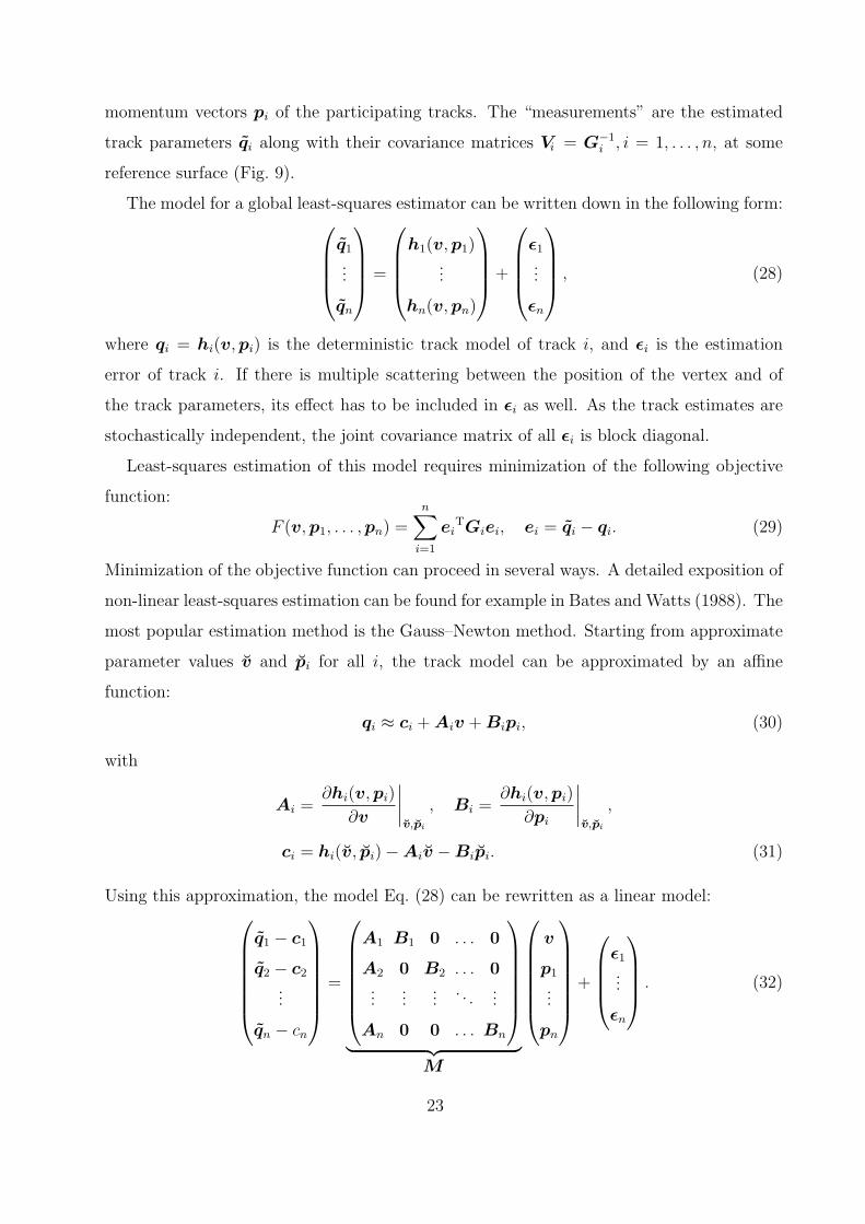
momentum vectors pi of the participating tracks. The “measurements” are the estimated

track parameters qi along with their covariance matrices Vi = G−1i , i = 1, . . . , n, at some

reference surface (Fig. 9).

The model for a global least-squares estimator can be written down in the following form:

q1

...

qn

=

h1(v,p1)...

hn(v,pn)

+

ε1...

εn

, (28)

where qi = hi(v,pi) is the deterministic track model of track i, and εi is the estimation

error of track i. If there is multiple scattering between the position of the vertex and of

the track parameters, its effect has to be included in εi as well. As the track estimates are

stochastically independent, the joint covariance matrix of all εi is block diagonal.

Least-squares estimation of this model requires minimization of the following objective

function:

F (v,p1, . . . ,pn) =n∑

i=1

eiTGiei, ei = qi − qi. (29)

Minimization of the objective function can proceed in several ways. A detailed exposition of

non-linear least-squares estimation can be found for example in Bates and Watts (1988). The

most popular estimation method is the Gauss–Newton method. Starting from approximate

parameter values v and pi for all i, the track model can be approximated by an affine

function:

qi ≈ ci +Aiv +Bipi, (30)

with

Ai =∂hi(v,pi)

∂v

∣∣∣∣v,pi

, Bi =∂hi(v,pi)

∂pi

∣∣∣∣v,pi

,

ci = hi(v, pi)−Aiv −Bipi. (31)

Using this approximation, the model Eq. (28) can be rewritten as a linear model:

q1 − c1

q2 − c2

...

qn − cn

=

A1 B1 0 . . . 0

A2 0 B2 . . . 0...

......

. . ....

An 0 0 . . . Bn

︸ ︷︷ ︸M

v

p1

...

pn

+

ε1...

εn

. (32)

23

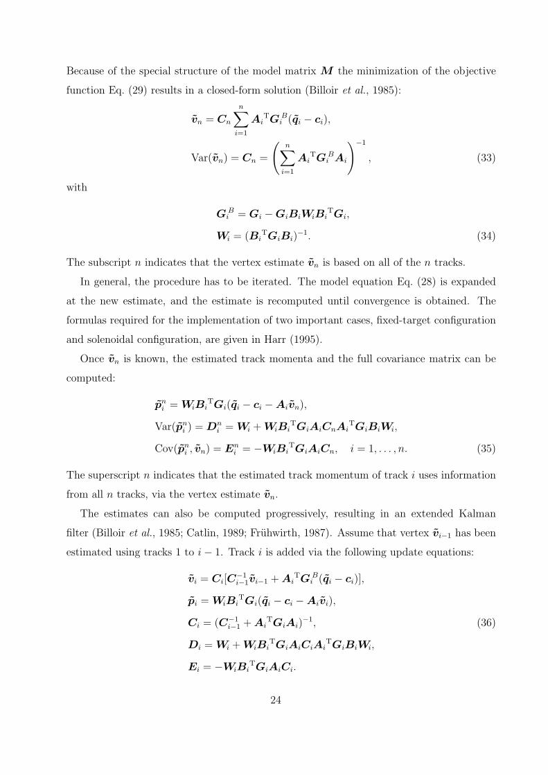
Because of the special structure of the model matrix M the minimization of the objective

function Eq. (29) results in a closed-form solution (Billoir et al., 1985):

vn = Cn

n∑

i=1

AiTGi

B(qi − ci),

Var(vn) = Cn =

(n∑

i=1

AiTGi

BAi

)−1

, (33)

with

GiB = Gi −GiBiWiBi

TGi,

Wi = (BiTGiBi)

−1. (34)

The subscript n indicates that the vertex estimate vn is based on all of the n tracks.

In general, the procedure has to be iterated. The model equation Eq. (28) is expanded

at the new estimate, and the estimate is recomputed until convergence is obtained. The

formulas required for the implementation of two important cases, fixed-target configuration

and solenoidal configuration, are given in Harr (1995).

Once vn is known, the estimated track momenta and the full covariance matrix can be

computed:

pni = WiBiTGi(qi − ci −Aivn),

Var(pni ) = Dni = Wi +WiBi

TGiAiCnAiTGiBiWi,

Cov(pni , vn) = Eni = −WiBi

TGiAiCn, i = 1, . . . , n. (35)

The superscript n indicates that the estimated track momentum of track i uses information

from all n tracks, via the vertex estimate vn.

The estimates can also be computed progressively, resulting in an extended Kalman

filter (Billoir et al., 1985; Catlin, 1989; Fruhwirth, 1987). Assume that vertex vi−1 has been

estimated using tracks 1 to i− 1. Track i is added via the following update equations:

vi = Ci[C−1i−1vi−1 +Ai

TGiB(qi − ci)],

pi = WiBiTGi(qi − ci −Aivi),

Ci = (C−1i−1 +Ai

TGiAi)−1, (36)

Di = Wi +WiBiTGiAiCiAi

TGiBiWi,

Ei = −WiBiTGiAiCi.

24

Apart from small numerical effects, the final result does not depend on the order in which

the tracks are added. The latter is therefore arbitrary.

The smoother associated to this filter is tantamount to recomputing the track momenta

using the last vertex estimate vn, i.e. Equations (35). For implementations of the full

Kalman filter formalism in the LHC experiments ATLAS and CMS, see Wildauer (2006)

and Waltenberger (2004).

Using the estimated vertex position and track momenta, the estimated track parameters

can be updated to:

qni = h(vn, pni ),

Var(qni ) = BiWiBiT + Vi

BGiAiCnAiTGiVi

B, (37)

with

ViB = Vi −BiWiBi

T. (38)

The updated track parameters are no longer independent.

The χ2 statistic of the final estimate is given by

χ2 =n∑

i=1

riTGiri, (39)

with the residuals ri = qi − qni . It can be used to test the vertex hypothesis, i.e. the

correctness of the model Eq. (28). If the test fails, however, there is no information about

which track(s) may have caused the failure.

The estimated track parameters qi are frequently given at the innermost detector surface

or at the beam tube. If the qi are propagated to the vicinity of the presumed vertex, the

vertex estimation can be speeded up by applying some approximations, especially if the

magnetic field is sufficiently homogeneous.

The “perigee” parametrization for helical tracks was introduced in Billoir and Qian

(1992), with a correction in Billoir and Qian (1994). The track is parameterized around

the point of closest approach (the perigee point vP) of the helix to the z-axis. The variation

of transverse errors along the track is neglected in the vicinity of the perigee, and track di-

rection and curvature at the vertex are assumed to be constant. The approximate objective

function of the vertex fit can then be written entirely in terms of the perigee points:

F (v) =n∑

i=1

(viP − v)T Ti (vi

P − v), (40)

25

where Ti is a weight matrix of rank 2. The vertex estimate is then

v =

(n∑

i=1

Ti

)−1( n∑

i=1

TiviP

). (41)

The Jacobians required to compute the Ti are spelled out in Billoir and Qian (1992, 1994).

For an implementation in ATLAS, see Piacquadio et al. (2008); Wildauer (2006).

A further simplification was proposed in Karimaki (1997). The track is approximated by a

straight line in the vicinity of the vertex. The estimated track parameters are transformed to

a coordinate system the x-axis of which is parallel to the track. The vertex is then estimated

by minimizing the sum of the weighted transverse distances of the tracks to the vertex. The

resulting objective function has the same form as in Eq. (40), again with weight matrices

of rank 2. The estimate is exact for straight tracks. The method has been implemented in

CMS (Waltenberger, 2004).

2. Robust vertex fitting

In experimental reality vertex candidates as produced by the vertex finder are often

contaminated by outliers. Outliers can be broadly classified into two categories. In the first

category are mismeasured tracks, i.e. tracks for which the deviation of the estimated track

parameters from the true track parameters is larger than indicated by the covariance matrix

of the track. There may be several reasons for that, including extraneous observations

resulting from a mistake in the track finding, a wrong estimate of the material the track

has crossed, or a wrong estimate of the covariance matrix of an observation. In the second

category are extraneous tracks not belonging to the vertex at all, e.g. a primary track

attached by mistake to a secondary vertex, or a background track attached to either a

primary or a secondary vertex.

As in the case of track reconstruction, there are two different ways of dealing with outliers.

Either outliers are identified and removed, or the influence of outliers is reduced by using

robust estimators. Outliers can be identified by inspecting their χ2 increment with respect

to the vertex estimated from the other tracks:

χ2i =ri

TGiri + (qi − ci −Aivn)T·

GiBAi(Cn

i)−1AiTGi

B(qi − ci −Aivn), (42)

26

with Cni = Cn−Ai

TGiBAi, the covariance matrix of the vertex fitted from all tracks except

track i. If there are no outliers, χ2i is χ2-distributed with m = dim(q) − dim(v) degrees

of freedom. As outliers should give significantly larger values of χ2i , the latter can be used

to test for the presence of outliers. If there are several outliers, the fitted vertex is always

biased, even if one of the outliers is removed. In this case it is better to reduce the influence

of outliers already in the estimate itself, by constructing a robust estimator.

One of the earliest proposals for a robust vertex fit (Fruhwirth et al., 1996) is an M-

estimator with Huber’s ψ-function (Huber, 1981). It can be implemented as an iterated

re-weighted least-squares estimator. The initial vertex estimate is a plain least-squares

estimate. Then, for each track, the residuals are rotated to the eigensystem of the covariance

matrix of the track, and weight factors are computed according to:

wi =

1, |ri| ≤ cσi,

cσi/|ri|, |ri| > cσi,(43)

where ri is one of the residuals in the rotated frame, σi is the standard deviation in the

rotated frame, and c is the robustness constant, usually chosen between 1 and 3. The

weight factors are applied and the estimate is recomputed. The entire procedure is iterated

until convergence.

A similar kind of re-weighted least-squares estimator was proposed in Agakichiev et al.

(1997). The weights are computed according to Tukey’s bi-square function (Hampel et al.,

1986):

wi =

(1− r2

i /σ2i

c2

)2

, |ri| ≤ cσi,

0, otherwise,

(44)

where r2i is the squared residual of track i with respect to the vertex, σ2

i is its variance,

and c is again the robustness constant. The estimator is now equivalent to a redescending

M-estimator (Hampel et al., 1986), and therefore less sensitive to outliers than Huber’s

M-estimator. The same weights were proposed in Golutvin et al. (2000) for robust track

fitting.

Another obvious candidate for robust vertex estimation is the least trimmed squares

(LTS) estimator (Chabanat et al., 2005; D’Hondt et al., 2004; Rousseeuw and Leroy, 1987).

27

With the LTS estimator, the objective function of Eq. (29) is replaced by

F (v,p1, . . . ,pn) =

bhnc∑

i=1

eiTGiei, ei = qi − qi, (45)

where h is the user-defined fraction of tracks to be included in the estimate. Finding the

subset of tracks that minimizes F is a combinatorial problem, which makes the LTS estimator

much more difficult (and slower) to compute than the least-squares estimator. In addition,

the fraction h is fixed and has to be specified in advance. As a consequence, tracks are

thrown away even if there are no outliers, and the precision of the estimate suffers. Both

problems can be overcome by the introduction of the adaptive vertex estimator (see III.F).

3. Vertex finding by iterated fitting

The test on outliers based on the χ2 increment χ2i (see Eq. (42)) can be expanded to a full-

blown vertex finder, by recursively identifying and removing outliers (Speer et al., 2006c).

The algorithm has been dubbed “trimmed Kalman filter”, but should not be confused with

the least trimmed squares (LTS) estimator (see II.D.2).

First, all input tracks are fitted to a common vertex, using a standard least-squares

estimator (see II.D.1). The χ2 increment is computed for all tracks, the track with the

largest increment is removed from the vertex, and the vertex is refitted. This procedure is

repeated until the χ2 increment of all tracks is below a given threshold. Once a track has

been rejected, it is not included again in the vertex.

When a vertex has been established, the entire procedure is repeated on the set of the

remaining tracks. The iteration stops when no vertex with at least two tracks can be

successfully fitted.

If there are no outliers and if all tracks are correctly estimated at the track fitting stage,

the χ2 increment is distributed according to a χ2-distribution with m = dim(q) − dim(v)

degrees of freedom. If the threshold mentioned above is set to the (1 − α)-quantile of the

χ2-distribution with m degrees of freedom, then under the null hypothesis of no outliers

the probability of rejecting a randomly chosen track is equal to α, and the probability of

rejecting the track with the largest χ2 increment is approximately equal to 1− (1− α)n, if

the number of tracks n is large enough so that the correlations between the χ2 increments

can be neglected.

28

If there are outliers, the χ2 increments are no longer χ2-distributed, and the probability

of rejecting a randomly chosen good track may be well above α. The respective probabilities

of falsely rejecting good tracks and correctly identifying outliers can no longer be calculated

analytically and have to be determined by simulation studies.

The iterative identification of outliers is therefore a lengthy and somewhat unreliable

procedure, especially if there are several outliers, resulting in a severe bias on the estimated

vertex position. These problems can be overcome by employing not a least-squares estimator,

but an adaptive estimator in each stage of the iteration (see III.F).

III. ADAPTIVE METHODS

The first attempt to equip track reconstruction methods with adaptive behaviour was

the application of the Hopfield network to track finding (Denby, 1988; Peterson, 1989).

As it turned out to be difficult to embed the correct physical track model into the Hopfield

network, the next step was the elastic arms or deformable template algorithm (Ohlsson et al.,

1992), and a related method called elastic tracking (Gyulassy and Harlander, 1991). At this

point the traditional boundaries between pattern recognition (track finding) and parameter

estimation (track fitting) started to dissolve. Both methods, however, required numerical

minimization of a complicated energy function. The realization that an alternative way of

minimization was provided by the EM algorithm (Dempster et al., 1977) then paved the way

to adaptive least-squares estimators in general, and to an adaptive version of the Kalman

filter in particular (Fruhwirth and Strandlie, 1999). Even the concept of annealing, native

to the world of neural networks and combinatorial optimization, could be transplanted in a

natural way into the world of stochastic filters. As vertex reconstruction is similar to track

reconstruction in many respects, adaptive methods developed for track finding and fitting

could be applied to vertex finding and fitting almost one-to-one.

Adaptive methods for track and vertex reconstruction tend to have a certain set of features

in common. The most salient ones are:

• After being initialized at some position, the track or vertex moves during an iterative

procedure due to some defined dynamical scheme. The dynamical scheme often uses

the information from the data several times during the iterations. This can also be

29

regarded as a sequential exploration of several hypotheses about the correct values of

the set of parameters describing the track or vertex.

• The observations — detector hits in the case of track fitting, reconstructed tracks

in the case of vertex fitting — can also have a weight attached to them, potentially

depending on the positions of other observations, thereby opening up the possibility of

soft assignment of the observations to the track or vertex. In the case of track fitting,

sets of mutually exclusive observations, e.g. several hits in the same detector layer,

can compete for inclusion in the track in the sense that hits close to the track tend to

downweight the influence of hits that are further away in the same detector layer.

• The dynamics of the track or vertex can often be regarded as an iterative strategy for

locating the minimum of an energy hyper-surface in the space of the track or vertex

parameters. This energy surface often has several local minima. In order to increase

the probability of reaching the global minimum, some of the methods introduce the

concept of temperature and annealing. Typically, an algorithm is initiated at a high

temperature, and the temperature parameter is decreased (“cooled”) during the iter-

ations. The effect is that the energy surface is smoothed out at high temperatures,

whereas the original structure of the energy landscape shows up in the late stages of

the iterations, when the temperature is low.

• A non-linear filter can explore a set of track or vertex hypotheses in parallel rather

than in sequence. The final result is calculated by collapsing the surviving hypotheses

into a single Gaussian distribution. The concepts of weights, soft assignment and

competition are therefore also relevant for non-linear filters.

A. Hopfield neural networks

Artificial neural networks (e.g. Hertz et al., 1991) constitute a computational paradigm

which is by now well established. Such networks are used in a range of different application

areas, for instance within pattern classification and combinatorial optimization problems.

The first application in high-energy physics dates back to 1989. Earlier reviews of the

applications of neural networks in high-energy physics can be found in Denby (1999); Kisel

et al. (1993).

30

For the solution of combinatorial optimization problems Hopfield networks (Hopfield,

1982) have emerged as particularly powerful tools. The standard dynamics of a Hopfield

network:

Si = sgn

(∑

j

TijSj

), (46)

where Tij is the connection weight between neuron i and neuron j and the sign function

sgn (x) is taken to be:

sgn (x) =

1, x ≥ 0,

−1, x < 0,(47)

leads to a local minimum of the energy function:

E = −1

2

∑

i

∑

j

TijSiSj (48)

with respect to the configuration of the set of binary-valued neurons Si. The general

solution to the problem is tantamount to finding the global minimum of the energy function.

A benchmark problem in combinatorial optimization is the travelling salesman problem,

which asks for the shortest path through N cities positioned at a set of known coordinates.

In Hopfield and Tank (1985) the travelling salesman problem was formulated as a minimiza-

tion problem of an energy function of a Hopfield network. Since the local minimum found

by the standard network dynamics can provide solutions quite far from the desired global

optimum, it was suggested to use a smooth update function, the hyperbolic tangent, inspired

by mean field theory from statistical mechanics. The mean field theory update equations

were rigorously derived by means of a saddle point approximation in Peterson and Anderson

(1987). The main idea behind this approximation is that the behaviour of the the partition

function Z,

Z =∑

S

e−E(S)/T , (49)

where S = S1, S2, ..., SN is a configuration of the N neurons in the network, is dominated

by the low-energy configurations of E(S). These configurations are searched for by first

replacing the sum over different configurations S = ±1 by integrals over continuous variables

U and V , giving

Z = c∏

i

∫ ∞

−∞dVi

∫ i∞

−i∞dUie

−E′(V ,U ,T ), (50)

31

where c is a normalization constant and the effective energy E ′ is given by

E ′(V ,U , T ) =E(V )

T+∑

i

[UiVi − ln (coshUi)] . (51)

The saddle points of Z are found by requiring that the partial derivatives of E ′ with respect

to both mean field variables Ui and Vi are zero, giving the update equations

Vi = tanh

(∑

j

TijVj/T

). (52)

The energy landscape of E ′ is smoother than that of the original energy E, particularly at

high temperatures T . The strategy of finding low-energy configurations is thus to initiate the

search at a high temperature and iterate (52) until convergence. The temperature is lowered,

and a new minimum configuration of the mean field variables is found, starting out from

the configuration obtained by the previous iteration. The whole procedure is repeated at

successively lower temperatures, approaching the zero-temperature limit in the end. In this

limit, the mean field equations reduce to the standard dynamics of the Hopfield network.

Since the mean field equations are solved at a sequence of decreasing temperatures, the

procedure is called mean field annealing.

It was realized independently by Denby (1988) and Peterson (1989) that the problem of

finding track candidates in a high-energy physics particle detector could be formulated as

the problem of minimizing an energy function of the Hopfield type. In this model, called the

Denby–Peterson network, the neurons correspond to links between measurements in adjacent

detector layers, and the weights quantify the probability of two adjoining links belonging to

the same track. If two such adjoining links point in approximately the same direction, the

energy is decreased; if two links start from or end up in the same measurement, the energy

is increased. An overall constraint, limiting the total number of active neurons to the overall

number of measurements, is also included in the energy function. The network is run to

convergence with mean field annealing. Fig. 10 shows an example of a Denby–Peterson

network in various stages of its evolution. At the end some shortcomings, such as missing or

illegal neurons and incorrect choices, can be observed. Of course the Hopfield dynamics is

just one way of minimizing the energy function. Alternatives to mean field annealing have

been explored but found to be inferior (Diehl et al., 1997).

The first experimental implementation of a Hopfield network was done in the ALEPH

experiment (Stimpfl-Abele and Garrido, 1991) and found to give results compatible with

32

those produced by the standard track finder used in the experiment. A simplified version of

a Hopfield network has also been tested on real data from the ARES spectrometer (Baginyan

et al., 1994). More recently, the method has been tried on simulated data from the ALICE

experiment (Badala et al., 2003, 2004). Used in combination with the standard, Kalman-

filter based track finding procedure, it was shown to increase the track finding efficiency as

compared to a stand-alone application of the Kalman filter.

B. Elastic nets and deformable templates

An alternative solution to the travelling salesman problem is the application of the elastic

net method (Durbin and Willshaw, 1987). In this method, the initial path is a smooth curve,

which in general does not pass through any of the cities. By an iterative procedure, the path

is gradually deformed through the influence of two different forces, whose relative strengths

are governed by two constants α and β. If the coordinates of city i are given by xi and

the coordinates of a typical point j along the path are given by yj, the change ∆yj in an

iteration is

∆yj = α∑

i

wij (xi − yj) + βK (yj+1 − 2yj + yj−1) , (53)

where K is a constant. One of the forces attracts the path toward the cities, whereas the

other one tries to minimize the total length of the path. The coefficient wij is the strength

of the connection between city i and point j. It is normalized:

wij =ϕ (|xi − yj| , K)∑k ϕ (|xi − yk| , K)

. (54)

If ϕ (d,K) is taken to be Gaussian:

ϕ (d,K) = e−d2/2K2

, (55)

an energy function E can be defined:

E =− αK∑

i

ln

(∑

j

ϕ (|xi − yj| , K)

)

+ β∑

j

|yj+1 − yj|2 , (56)

such that the update of the position yj can be regarded as a gradient descent of the energy

function in the coordinate space of yj:

∆yj = −K ∂E

∂yj. (57)

33

The value of K is lowered during the iterations, causing the path to eventually pass through

all of the cities. On problems with a quite large number of cities, the elastic net method is

superior to the Hopfield network approach (Durbin and Willshaw, 1987).

The elastic net method has been successfully applied to track fitting in a drift tube

detector in the NEMO experiment (Kisel et al., 1997). For this application, three different

forces are acting during the iterations. One draws the track to the edge of the drift circle

defining the possible positions of the measurement in the tube, the other smooths out the

track, and the third attracts the two lines constituting the envelope of the track toward each

other. An example is shown in Fig. 11.

An application of the elastic net to vertex finding is described in Kisel et al. (1997).

As the vertex can be anywhere in a big target (diameter ≈ 10 cm) there is no good initial

approximation to the vertex position. The vertex is therefore defined as the center of the

area with maximum track density. The vertex finder is based on an elastic ring and uses

two types of forces: attraction of the ring to all tracks, shifting toward the area with high

track density; and attraction to the nearest tracks, localizing the vertex region.

More recently, the elastic net method has also been applied to ring finding in a ring

imaging Cerenkov detector in the CBM experiment (Gorbunov and Kisel, 2005, 2006).

A very important generalization of the elastic net method has been developed in Yuille

(1990), formulating the travelling salesman problem as an assignment problem, with an

energy function containing binary assignment variables Vij. These variables are equal to one

if city i is assigned to point j, and zero otherwise. In order to assign a city to only one

point, the constraint∑

j Vij = 1 is introduced. The energy function E reads:

E [Vij , yj] =∑

ij

Vij |xi − yj|2

+ ν∑

j

|yj − yj+1|2 , (58)

where ν is a positive constant. Finding a minimum of E with respect to all possible and

allowed values of Vij and yj is prohibitively difficult. A more feasible approach is

to consider the average behaviour of the assignment problem by assuming a Boltzmann

distribution for the states of the system:

P [Vij , yj] =e−E[Vij,yj]/T

Z, (59)

34

where the partition function Z is given by:

Z =∑

Vij,yj

e−E[Vij,yj]/T . (60)

Summing over all allowed configurations of Vij, the partition function becomes:

Z =∑

yj

e−Eeff[yj]/T , (61)

with the effective energy:

Eeff [yj] =− T∑

i

ln

(∑

j

e−|xi−yj |2/T

)

+ ν∑

k

|yk − yk+1|2 . (62)

This is the same as the energy function of the elastic net method (Durbin and Willshaw,

1987). As the sought minimum configuration of the system dominates the behaviour of the

partition function in the low-temperature limit, a feasible strategy is to initiate the search

at a large temperature and find the minimum of the effective energy. The temperature

is lowered, and a new minimum is found, starting out at the values of yj found by the

previous minimization. The procedure is repeated at successively lower temperatures, taking

the zero-temperature limit in the end. This procedure is equivalent to the elastic net method

iterated at successively lower values of the constant K (Durbin and Willshaw, 1987). With

the introduction of a parameter interpreted as temperature, such a procedure can be regarded

as an annealing procedure. Being non-random — in contrast to the stochastic strategy called

simulated annealing (Kirkpatrick et al., 1983) — it is an example of a deterministic annealing

procedure.

The Hopfield network algorithm (Hopfield and Tank, 1985) can also be derived us-

ing Eq. (58) by considering the average behaviour of yj instead (Yuille, 1990). Such

a strategy gives a new energy only dependent on Vij, which is very similar to the energy

function of Hopfield and Tank (1985). This establishes the close connection between the

elastic net method and the neural network approach.

The track reconstruction task has in Ohlsson et al. (1992) been formulated as an assign-

ment problem in a way very similar to the approach described in Yuille (1990). In this

so-called elastic arms approach, measurements i are assigned to template tracks or arms a

35

by the binary decision units Sia under the constraint that each measurement is assigned

to at most one arm a. The energy function reads:

E [Sia, qa] =∑

ia

SiaMia + λ∑

i

(∑

a

Sia − 1

)2

, (63)

where Mia is the squared distance from measurement i to the track parameterized by the

track parameter vector qa. The second term imposes a penalty if a measurement is not

assigned to any track. Following exactly the same strategy as described for the travelling

salesman problem above, the states of the system are assumed to obey a Boltzmann distri-

bution, and an effective energy Eeff is obtained by summing over all possible configurations

of the assignment variables,

Eeff [qa] = −T∑

i

ln

(e−λ/T +

∑

a

e−Mia/T

). (64)

As before, the system is initiated at a large temperature with a certain set of values of the

parameters of the arms. Successive minimizations are performed at a sequence of decreasing

temperatures, stopping at a temperature close to zero. The minimization strategy at a given

temperature is equivalent to the gradient descent procedure of Durbin and Willshaw (1987).

Visually, this procedure amounts to a set of arms or template tracks being attracted to the

measurements created by the charged particles during the annealing. At low temperatures,

the arms settle in the vicinity of these measurements, and measurements too far from the

arm have no effect on the final estimate of the track parameters due to the cutoff parameter

λ.

The algorithm has been extended to deal with left-right ambiguities in drift tube detec-

tors (Blankenbecler, 1994), and improved minimization schemes using the Hessian matrices

have been introduced (Ohlsson, 1993). The first test in an LHC scenario was done in Lind-

strom (1995). Applied to track reconstruction in the Transition Radiation Tracker subsystem

of the ATLAS detector (Aad et al., 2008), the arms were initiated by the output of a Hough

transform track finding procedure. The elastic arms algorithm was then run in order to

resolve the left-right ambiguities and settle on the final estimates of the track parameters.

A similar approach, called the elastic tracking algorithm, was developed in Gyulassy

and Harlander (1991). The basic idea is to interpret the classical Radon transform as an

interaction energy between the measurements in a tracking detector and a template track.

36

The minimum of the interaction energy with respect to the parameters of the template

track defines the solution to the problem. Similar to the elastic arms algorithm, an iterative

annealing procedure is followed in order to avoid local minima of the energy function. A

comparison between the Denby–Peterson network and the elastic tracking algorithm is shown

in Fig. 12.

The interaction energy RV as presented in Gyulassy and Harlander (1991) can in principle

handle continuous charge distributions, i.e. situations where the charged particle potentially

has ionized several neighbouring basic detector units. Usually, the information from such

neighbouring units is compressed into an effective measurement before track reconstruction

starts, implicitly discretizing the data. For discretized data the interaction energy is defined

in terms of a sum over measurements i and tracks a:

RV (q, I) = −∑

ia

V (Mia, I) , (65)

where V is an interaction potential and I is the iteration number. In Gyulassy and Harlander

(1991) a Lorentzian potential of the following form was suggested:

V (Mia, I) =w2 (I)

Mia + w2 (I), (66)

where w2 is chosen quite large in the beginning of the iterations in order to smooth out

the energy surface; asymptotically it should reach a value compatible with the standard

deviation of the measurement error. The algorithm has been tested out in a TPC-like

scenario with nearby and overlapping tracks (Gyulassy and Harlander, 1992). Working on

non-clustered data with realistic charge fluctuations, sub-pad multiple track resolutions were

obtained.

A potential disadvantage with the deformable templates approach is the high computa-

tional complexity. An attempt to speed up the elastic arms algorithm was made by formu-

lating it as a single-track algorithm (Fruhwirth and Strandlie, 1999). At the same time, it

was generalized in order to cope with an arbitrary number of competing measurements in

the same detector layer. It was shown in this paper that despite the simplification to the

single-track formulation, further computational load nevertheless had to be introduced in

order to achieve optimal performance, as advanced approaches such as quasi-Newton meth-

ods are needed in the final iteration for locating the global minimum of the energy function

with satisfactory accuracy. Another disadvantage is the need of a parametric model of the

37

track, which limits the application to experimental scenarios with vanishing or homogeneous

magnetic fields, and negligible material effects such as energy loss and multiple scattering.

Track reconstruction and vertex reconstruction have many features in common. It is

therefore not surprising that the deformable template method has been extended to the

problem of vertex finding (Stepanov and Khanov, 1997). Simultaneous track and vertex

finding with deformable templates was proposed in Haas (2000).

In the most general case, vertex finding starts with K tracks and N vertex templates.

Each template is a collection of the following elements: the vertex position vn, K binary

decision units Vnk, the momentum vectors pnk at vertex n of all tracks, and the estimated

track parameters qk, where 1 ≤ k ≤ K. The energy function reads:

E [Vnk, vn, pnk, qk] =

=N∑

n=1

K∑

k=1

VnkMnk + λK∑

k=1

(N∑

n=1

Vnk − 1

)2

, (67)

where Mnk is a measure of distance between vertex template n and track k. The second

term in Eq. (67) imposes a penalty when a track is not matched to exactly one vertex. The

distance Mnk is chosen as the χ2 statistic:

Mnk = rnkTGkrnk, (68)

where rnk = qk − hk(vn,pnk) is the residual of track k with respect to vertex template n

(see Eq. (28)), andGk is the inverse covariance matrix of track k. If there is prior information

that track k cannot be associated with vertex n, the corresponding decision unit Vnk can be

frozen to 0.

In Stepanov and Khanov (1997) the energy function was minimized iteratively, by alter-

nating two steps. In the first one the energy function was minimized with respect to the

continuous variables vn and pnk, using gradient descent. In the second step, the weights

were updated according to:

Vnk =e−Mnk/T

e−λ/T +∑N

i=1 e−Mik/T

, (69)

with a temperature parameter T . In the example presented in Stepanov and Khanov (1997),

the starting temperature was chosen to be about 1 and slightly decreased during the itera-

tions. The penalty term λ was chosen to be large (≈ 50) and slightly decreased as well in

the course of the minimization.

38

C. Gaussian-sum filter

As seen in the previous subsection, elastic tracking approaches can be used to resolve

ambiguities and downweight noise. For instance, in the elastic arms approach the parameter

λ plays the role as a cutoff parameter, since measurements with a squared distance to the

arm larger than λ have virtually no effect on the final estimates of the track parameters.

A first attempt to achieve a similar downweighting effect within a filtering approach took

as a starting point a two-component Gaussian-mixture description of the measurement error,

the narrow component representing true measurements and a wider component representing

outliers (Fruhwirth, 1995; Guttman and Pena, 1985; Lin and Guttman, 1993). The update

of the track parameters and the covariance matrix is obtained in a Bayesian spirit as the

mean and covariance matrix of the posterior distribution, resulting in a weighted sum of the

output of two Kalman filters. This collapsed state vector is then propagated to the next

detector layer containing a measurement.

The procedure was later, following Kitagawa (1989, 1994), generalized to a full Gaussian-

sum filter (GSF; Fruhwirth, 1997). In the full GSF, both measurement noise and stochastic

material effects such as multiple scattering and energy loss by bremsstrahlung are mod-

elled as Gaussian mixtures. The posterior distribution is not collapsed after every update,

and the GSF takes the form of a set of Kalman filters running in parallel. Each time a

Gaussian-mixture probability density function with M components is encountered during

the reconstruction procedure, the posterior distribution is still a Gaussian mixture but con-

taining M times as many components as the prior distribution.

Let x denote the track state at a material layer or a measurement layer, and let its prior

distribution be a mixture of K multivariate Gaussians. The mixture density is completely

specified by its weights, mean vectors, and covariance matrices:

f(x) =K∑

k=1

πk ϕ(x;xk,Ck),K∑

k=1

πk = 1. (70)

If the state is at a material layer, and the process noise (e.g. multiple scattering or

bremsstrahlung) is modelled by a Gaussian mixture with M components:

g(x) =M∑

m=1

wm ϕ(x;µm,Qm),M∑

m=1

wm = 1, (71)

39

the posterior density of the state vector is given by a mixture of all pairwise convolutions:

p(x) =K∑

k=1

M∑

m=1

πk wm ϕ(x;xk + µm,Ck +Qm). (72)

If the state is at a measurement layer, and the measurement error is modelled by a Gaussian

mixture with M components:

h(m) =M∑

m=1

ωm ϕ(m;Hx+ cm,Vm),M∑

m=1

ωm = 1, (73)

the posterior density of the state vector is computed using Bayes’ theorem:

p(x) =K∑

k=1

M∑

m=1

pkm ϕ(x;xkm,Ckm), (74)

with

xkm = xk +CkmHTV −1

m (m− cm −Hxk),

Ckm =[C−1k +HTV −1

m H]−1

, (75)

pkm ∝ πk ωm ϕ(m;Hxk + cm,Vm +HCkHT).

The constant of proportionality is determined by the constraint

K∑

k=1

M∑

m=1

pkm = 1.

This procedure leads to an exponentially increasing number of components in the poste-

rior distributions, and for practical purposes the maximum number of components has to be

limited. Depending on the application, this can be achieved by keeping the N components

with largest posterior weights, or by merging components being close in parameter space,

closeness defined by an appropriate similarity metric.

A GSF has been developed for the resolution of drift time ambiguities by modelling

the measurements as a two-component mixture with different means, corresponding to the

two potential positions of the measurement, but equal standard deviations (Fruhwirth and

Strandlie, 1999). A potential drawback of this approach is the sensitivity to wrong or noisy

measurements, particularly in the early phases of the filter where the track parameters

are poorly defined. Good initialization of the track parameters is therefore essential. The

method has been made more robust by introducing the concept of a missing hit (Fruhwirth

40

and Strandlie, 2006), which implies that an additional component is created whenever a

detector unit with a measurement is reached. This additional component is transported

directly through the detector unit and corresponds to a measurement missing due to detector

inefficiencies or being wrong, for example because of track finding inefficiencies.

A totally different application of the GSF is the treatment of bremsstrahlung energy loss of

electrons, which follows a highly non-Gaussian distribution. The Bethe–Heitler model (Bethe

and Heitler, 1934) of this distribution has been approximated in terms of Gaussian mixtures

for a range of radiation thicknesses (Fruhwirth, 2003). A proof-of-principle study was re-

ported in Fruhwirth and Fruhwirth-Schnatter (1998), and the first experimental application

was made and tested out on simulated data in the CMS experiment (Adam et al., 2005).

A comparison of the GSF with the standard Kalman filter (KF), using electron tracks from

the full CMS simulation, is presented in Fig. 13. The figure shows the distribution of the

normalized difference between estimated and true momentum, both without and with a ver-

tex constraint. The distribution of the GSF estimates has a significantly narrower core than

the KF distribution, although the tails are slightly longer.

The GSF was also implemented in the ATLAS experiment at the LHC and was shown, at

least for simulated data, to improve the momentum resolution as compared to the standard

Kalman-filter based algorithm (Aad et al., 2008).

A related algorithm, the dynamic-noise-adjustment (DNA) method (Kartvelishvili, 2007),

was shown to yield similar results with less computational load. It can be regarded as a

simplified version of the GSF. It makes a selection between a radiating and a non-radiating

component at each material layer and thereby propagates only a single component through

the detector.

Yet another application of the GSF has been found for the task of discriminating between

different types of material encountered during a track reconstruction procedure (Strandlie

and Fruhwirth, 2006a). In a detector setup with complex structures consisting of different

types of material, the standard approach is to create a reconstruction geometry with averaged

material properties. The GSF approach is to create one component for each of the different

types of material present in the structure and using the measurements a posteriori to decide

which of the types of material the particle actually went through.

If the vertex fit is formulated as a Kalman filter (see II.D.1), the latter can be generalized

to a Gaussian-sum filter by taking a similar approach as in track fitting (Fruhwirth and

41

Speer, 2004; Speer and Fruhwirth, 2006). As multiple scattering usually is absent in vertex

fitting, it is the observations, i.e. the estimated track parameters of a previous track fit,

that are modelled by Gaussian mixtures. The Gaussian-sum filter can be useful in two

scenarios. In many cases the distribution of the estimation errors shows a Gaussian core

and non-negligible tails. These tails reflect imperfections of the track reconstruction. They

may be caused by the track finder picking up wrong hits or distorted hits, or by deficiencies

in the material description, the calibration, or the alignment of the tracking device. In this

first scenario, the components of the Gaussian in general have the same mean vector, but

different covariance matrices. In the second scenario the track itself has been estimated by

a GSF, for instance because it is an electron track. In this second scenario, the components

have different mean vectors and very likely also different covariance matrices. The most

general mixture model for the estimated track parameters is therefore the following one:

f(q) =M∑

m=1

ωm ϕ(q; qm,Vm),M∑

m=1

ωm = 1. (76)

In the first scenario, the joint mean vector of all components is the actual estimate q.

If a track is added to the vertex in the course of the GSF, the prior distribution of the

vertex position is itself a Gaussian mixture:

g(x) =K∑

k=1

πk ϕ(v;vk,Ck),K∑

k=1

πk = 1. (77)

After the track has been added, the joint posterior of the vertex position and the track

momentum is a mixture with M ·K components:

p(v,p) =K∑

k=1

M∑

m=1

pkm ϕ((v,p); (vkm,pkm),Ωkm). (78)

The calculation of the components weights pkm, the mean vectors (vkm,pkm) and the joint

covariance matrices Ωkm is analogous to Eq. (75). For more details about the limitation

of the number of components, smoothing, and results with simulated data, see Speer and

Fruhwirth (2006).

42

D. EM algorithm and adaptive track fitting

In the single-track formulation of the elastic arms algorithm, the energy function E reads

E (Sk, sik , q) =∑

k

[Sk

(nk∑

i=1

sikMik

)+ λ (Sk − 1)2

], (79)

where the sum over k denotes sum over layers, nk is the number of measurements in layer k

(including double-counting due to potential left-right ambiguities in a drift tube detector),

and Mik is the squared distance from measurement i in layer k to the single arm or track

under consideration. The track parameter vector is denoted by q. The binary assignment

variables Sk and sik are either 0 or 1, and the sik obey the constraint∑nk

i=1 sik = 1. The

variable Sk is 0 if all measurements in layer k are regarded as noise and 1 if one of them is

not. The effective energy becomes in this case:

Eeff (q) = −T∑

k

ln

(nke

−λ/T +

nk∑

i=1

e−Mik/T

). (80)

As mentioned earlier, the minimization of this non-quadratic energy function in general

requires time-consuming, non-linear approaches in order to locate the minimum with a

required accuracy. It was realized by Ohlsson et al. (1992) and Yuille et al. (1994) that the

EM algorithm is an alternative way of minimizing such energy functions. The EM algorithm

proceeds by alternating expectation and minimization steps and is guaranteed to converge

to a — possibly local — minimum of the energy function (Dempster et al., 1977).

The expectation step calculates the average of the original energy function as given

in Eq. (79) over the assignment variables, conditioned on the current value q′ of the track

parameters. This defines the function:

Q (q|q′) =∑

Sk,sik

E (Sk, sik , q) · P (Sk, sik |q′) , (81)

where P (Sk, sik |q′) is the joint distribution of all assignment variables, given that the

track parameters are equal to q′. The result of the summation is (Fruhwirth and Strandlie,

43

1999):

Q (q|q′) =∑

k

(nk∑

i=1

Mike−M

′ik/T

nke−λ/T +∑nk

j=1 e−M ′

jk/T

+ λnke

−λ/T

nke−λ/T +∑nk

j=1 e−M ′

jk/T

)

=∑

k

(nk∑

i=1

Mikp′ik + λp′0k

), (82)

where the primed quantities refer to a track with parameters q′. The interpretation of p′ik is

the probability of measurement i in layer k being assigned to the track, whereas p′0k is the

probability that none of the measurements is assigned to the track.

In the minimization step the function Q is minimized with respect to the parameters q,

regarding the primed quantities as fixed. The last term in Eq. (82) is independent of q, so

the same result is obtained if

Q1(q|q′) =∑

k

nk∑

i=1

Mikp′ik (83)

is minimized with respect to the parameter vector q. The new value of the parameter vector

is used to re-calculate the assignment probabilities, and the function Q1 is again minimized.

These alternating expectation and minimization steps are repeated until convergence, and

the EM algorithm can be seen to amount to an iteratively re-weighted least-squares proce-

dure, where the weights are given by the assignment probabilities. The risk of reaching a

local minimum of the energy function can again be decreased by annealing the temperature

parameter T .

This is a very important result. Through the application of the EM algorithm, the

non-linear problem of minimizing a non-quadratic energy function is solved by iterated

minimizations of a quadratic energy function, which can be done by a linear least-squares

estimator. If the Kalman filter is chosen as the linear least-squares estimator, the elastic

arms algorithm becomes an iterated Kalman filter with annealing. The resulting algorithm

is called the deterministic annealing filter (DAF; Fruhwirth and Strandlie, 1999). It has

the additional advantage with respect to the standard formulation of the algorithm that

material effects such as energy loss and multiple scattering can be taken into account in a

straightforward manner. In addition, track models that do not have a simple parametric

form can also be dealt with, as the prediction step of the Kalman filter in general can consist

44

of track propagation through an inhomogeneous magnetic field. An example of the outcome

of a track fit using the DAF is shown in Fig. 14. In this example it is evident that annealing

helps to avoid local minima of the energy function.

On the other hand, the running of a weighted Kalman filter as part of one iteration

of the DAF can be regarded as a simplified version of a Gaussian-sum filter, where the

GSF state vector is collapsed after every update. The iteration procedure can be motivated

from a desire of overcoming the problem of insufficient information in the initial phase of

the GSF. The DAF is thus seen to build a bridge between approaches based on neural

networks/deformable templates and more classical approaches based on the application of

stochastic filters.

With the GSF analogy in mind, the assignment weights of the DAF can be made more

general than those arising from the elastic arms algorithm. In particular, they can take

into account the fact that competing observations need not have the same precision. As a

consequence they are similar to the GSF weights but do not include the covariance matrix

of the predicted state, since the track from the previous iteration is regarded as fixed during

an expectation step of the EM algorithm:

pik =ϕ(mik;Hkx

∗k|n,Vik)

c+∑nk

j=1 ϕ(mjk;Hkx∗k|n,Vjk), (84)

where ϕ is again the Gaussian probability density function, mik is measurement i in layer k,

Vik is the associated covariance matrix, x∗k|n is the smoothed prediction from the previous

iteration, and c is a cutoff term resembling the term containing λ in the elastic arms weights

given in Eq. (82). A further generalization of the calculations of the assignment weights

is presented in Strandlie and Zerubia (1999), allowing arbitrary probability distribution

functions of the measurement errors.

The multi-track formulation of the elastic arms algorithm is via the EM algorithm gen-

eralized to a multi-track formulation of the DAF. This algorithm, called the multi-track

filter (MTF; Strandlie and Fruhwirth, 2000), amounts to a set of iterated Kalman filters

running in parallel; see Fig. 15 for an illustration. As for the DAF with respect to the

single-track version of the elastic arms algorithm, decisive features are e.g. the ability of

taking material effects and inhomogeneous magnetic fields correctly into account.

The fact that the minimization of a non-quadratic energy function can be done by iterated

minimizations of a quadratic function has quite far-reaching consequences. The minimization

45

of the quadratic function can in principle be done by any relevant least-squares estimator.

For instance, in a two-dimensional detector setup where the track model is the arc of a

circle, a linear circle fit method based on a mapping to the Riemann sphere and fitting a

plane to three-dimensional measurements leads to an adaptive approach called the elastic

planes algorithm (Strandlie et al., 2000). Since the backbone method for fitting is a very

fast, approximate circle fit, the elastic planes algorithm is in Strandlie et al. (2000) shown to

be much faster than the DAF and equally precise, as long as the assumption of the purely

circular track model holds at least approximately.

Another important consequence is that the DAF and the MTF immediately can be trans-

lated into analogous methods for adaptive, iterated, linear estimation of vertices, as first sug-

gested in Strandlie (2000). Adaptive methods of vertex fitting are described in Section III.F.

E. Comparative studies

The DAF was first implemented for simulation studies in the barrel part of the ATLAS

Transition Radiation Tracker (Fruhwirth and Strandlie, 1999). The barrel TRT consists of

75 layers of drift tubes (straws). The layers as well as the tubes in each layer are separated by

about 6.8 mm. Because of the inherent left-right ambiguity of the drift time measurement,

most hits have a mirror hit. The DAF was compared in terms of precision and running time

to the following other methods: the Gaussian-sum filter (GSF), the elastic arms algorithm

(EAA), and the elastic tracking algorithm (ETA). Two different annealing schedules were

used for the DAF and EAA. In the “nominal schedule” the final value of the temperature

T corresponded to the actual standard error of the observations, whereas in the “frozen

schedule” the final value of T was smaller by a factor of nine. The result of the GSF

was computed in two ways, using either all components or only the best (most probable)

component. The ETA was implemented using either a Gaussian (ETA-G) or a Lorentzian

(ETA-L) potential. The results for tracks with mirror hits are shown in Table I. The

precision of the method is quantified by the relative generalized variance (determinant of

the covariance matrix) of the track parameters w.r.t. to the true ones, the baseline being

the DAF for tracks without mirror hits.

Some interesting conclusions may be drawn from the table. First, the mathematical

equivalence of the EAA and the DAF is illustrated by nearly identical results. The DAF

46

is, however, faster by almost a factor of two. Second, cooling the DAF below the nominal

standard deviation of the observations slightly deteriorates the precision. Third, using the

full posterior information of the GSF is slightly better than just using the most probable

component. The latter is equivalent to a combinatorial Kalman filter (see Section II.B.3).

The GSF is considerably slower than the other methods. Finally, the ETA is about as fast

as the EAA, but not competitive in terms of precision.

The robustness of the estimators was studied by contaminating the tracks with noise.

In each tube, the correct drift distance was replaced by a random drift distance with a

probability of ten percent. The results are shown in Table II.

It is evident that the performance of the GSF has deteriorated considerably, showing its

inherent lack of robustness. The precision of the ETA is again worse than the one of the

DAF, the Gaussian potential being somewhat less susceptible to the influence of the mirror

and noise hits.

The multi-track filter (MTF) was first studied in Strandlie and Fruhwirth (2000), using

pairs of tracks in the ATLAS barrel TRT. A typical pair of tracks, including all hits, mirror

hits and additional noise hits, is shown in Fig. 15. Four competition schemes were analyzed:

1. Competition between hits. In each layer, there is competition between all hits for each

track, but no competition between the tracks. This scheme is equivalent to the DAF.

2. Competition between tracks. In each layer, there is competition between all tracks

for each hit, but no competition between the hits. This scheme is equivalent to the

original formulation of the EAA (Ohlsson et al., 1992).

3. Global competition. In each layer, all tracks compete for all hits.

4. Competition between tracks and between mirror hits. This is a refinement of scheme 2,

specific for detectors with mirror hits.

With the MTF, the initial values of the track parameters play an important role. In order to

separate the effect of the initialization from the properties of the competition schemes, the

track parameters were initialized at their true values. Table III shows the relative generalized

variance of the four schemes for tracks with mirror hits and additional noise hits at various

noise levels. The baseline is a single-track fit of all tracks.

47

Scheme 1, the DAF, is consistently the least precise. Scheme 2 is also less precise than

schemes 3 and 4. Schemes 3 and 4 are comparable, but not entirely equivalent. At noise

levels below 20%, scheme 4 is better, whereas at higher noise levels scheme 3 is better. The

explanation is that scheme 4 implements a competition between a hit and its mirror hit,

whereas scheme 3 treats all hits in a layer in the same manner. If the dominant source of

ambiguity are mirror hits, scheme 4 is best equipped to deal with this situation. If, on the

other hand, noise hits are the dominant source, scheme 3 is better, being designed to cope

with additional noise hits.

Other studies, based on more detailed simulations, have been made in the CMS

Tracker (Speer et al., 2006b; Winkler, 2002). For track reconstruction in dense jets, the

DAF was shown to yield substantial improvements both in track parameter resolutions and

in the overall track quality with respect to the standard Kalman-filter based procedure. The

MTF provided resolutions similar to the DAF but gave better estimates of the track param-

eter covariance matrices in the most difficult situations, i.e. in the core of the jets with the

highest energy.

The possibility of applying adaptive algorithms such as the DAF and the GSF for track

reconstruction in scenarios with very large amounts of background and noise have been

addressed in a couple of feasibility studies (Fruhwirth and Strandlie, 2006; Strandlie and

Fruhwirth, 2006b). In these studies the robust version of the GSF, allowing for missing

observations, was used.

Two different experimental setups were studied. One of them (setup C) is an all-silicon

tracking detector, similar to the CMS Tracker at the LHC. The other one (setup A) is a

combined silicon/drift tube detector system, similar to the ATLAS Inner Detector at the

LHC. In both experiments, track finding was starting from seeds that were track segments

in the innermost parts of the detectors. These seeds consisted of measurements in three

consecutive layers with pixel resolution in setup C, whereas the seeds consisted of measure-

ments from seven consecutive layers (three with pixel resolution and four with silicon strip

resolution) in setup A. Track finding was then carried out in the ten outermost silicon strip

layers in setup C and in the 36 drift tube layers in setup A. In both cases the track fit

was carried out using the full information from all measurements in the track candidates,

including the seeds.

Results from the simulation experiments with setup C, similar to the CMS Tracker, are

48

shown in Fig. 16. Track finding was performed using either the combinatorial Kalman filter

(CKF) or the GSF, whereas the track fit was done either by a standard Kalman smoother

(KSM) or by the DAF. In addition to the correct measurements, noise was added with a

density of 3 hits per mm2 in the innermost silicon layer, decreasing inversely proportional

to the radius. In addition, the true hits were replaced by noise hits with a 30 % probability.

The results are shown as a function of the quality of the measurements constituting the

seeds. The pixel hits were distorted by increasing the width of the Gaussian smearing with

a scale factor k. Thus k = 1 gives perfect seeds, and increasing the value of k gives seeds

which are gradually deteriorated.

The efficiency of track finding is seen to be quite similar for all combinations of track

finding and track fitting methods. As expected, the performance gets worse as the quality

of the seeds decreases. The resolution is consistently, but not dramatically, better using the

DAF in the track fit as compared to the KSM. Track finding at a noise level of 10 hits per

mm2 in the innermost silicon layer was also studied (Fruhwirth and Strandlie, 2006), but

at this noise level track finding broke down completely, because almost all track candidates

found were just random collections of noise hits.

Results from the simulation experiments with setup A, similar to the ATLAS Inner Detec-

tor, are shown in Fig. 17. The performance is shown as a function of the maximum number

of components or branches kept by the GSF or the CKF. In addition to the same combi-

nations of track finding and track fitting methods as shown in Fig. 16, a fully DAF-based

combined track finding and fitting was tried out. In this case, the seed was extrapolated

through the entire volume of the drift-tube detector, and measurements in a band along the

extrapolated track constituted the track candidate used by the DAF track fit.

It can be seen that the track finding efficiency of the GSF is better than that of the CKF,

and that the accuracy of the DAF track fit is better than the KSM track fit. The efficiency

of the stand-alone DAF is by far the best in this case, as it finds several of the tracks not

being found by the CKF or GSF due to too many missing hits. The difference in accuracy

between the stand-alone DAF and the DAF track fit initiated by the CKF or GSF track

finding is also due to the larger track sample fitted by the stand-alone DAF, containing

tracks with more missing hits and thereby yielding less estimation accuracy.

The stand-alone DAF was also tried out in setup C, but gave a significantly smaller

efficiency than the other methods. The reason is the larger amount of material present in

49

a silicon-based detector as compared to a gaseous one, leading to more multiple scattering,

and the lower quality of the seeds. The first extrapolation through the entire detector can

then be quite far away from the real track, and with a lot of noise hits present, the DAF is

not able to recover.

In general, the stand-alone DAF seems to work best as compared to other methods when

initiated with high-quality seeds, and when used in detector setups with relatively little

material. This can be explained by the fact that the DAF uses information from the entire

set of measurements in the track candidate when calculating the assignment weights, and the

full power of this feature is utilized in situations with long-range propagation of information

from the measurements. With a significant amount of material present, the information

from measurements far away is blurred by multiple scattering, and the assignment power

decreases. In the track fit, however, the DAF seems at these noise levels to be the method

of choice in both experimental setups.

F. Adaptive vertex fitting

The deformable template method of vertex finding can be rewritten as an iterated re-

weighted least-squares estimator. In the case of a single vertex to be found, the algorithm

is called the adaptive vertex fit (AVF; Waltenberger, 2004; Waltenberger et al., 2007a).

The estimator can be interpreted both as an EM algorithm and as a redescending M-

estimator (Fruhwirth and Waltenberger, 2008). If the estimator is formulated as an adaptive

filter, the corresponding dynamical system has no process noise. In the light of the results

in Section III.E it can therefore be expected that the adaptive approach is particularly

appropriate to vertex fitting.

The AVF is an alternating sequence of two steps: estimation of the vertex position, and

computation of the track weights. If the estimator is enhanced by deterministic annealing,

the temperature parameter is decreased after every iteration. In the EM interpretation, the

weight of a track is the posterior probability of the track actually belonging to the vertex,

called the assignment probability.

The estimation can be performed by a Kalman filter or by any other least-squares estima-

tor, e.g. one of the simplified estimators described in II.D. The computation of the weight

50

of track k is a special case of Eq. (69):

wk =e−χ

2k/2T

e−χ2cut/2T + e−χ

2k/2T

, (85)

where χ2k is the weighted distance of track k from the current vertex position, χ2

cut is a

cutoff, and T is the temperature parameter. The shape of the weight function for a cutoff

of χ2cut = 9 and different values of the temperature is shown in Fig. 18. The weight is equal

to 0.5 if χ2 = χ2cut. At low temperatures the weight function approaches a step function,

resulting in a yes/no decision about the assignment of the track to the vertex.

As mentioned above, the AVF can also be interpreted as a redescending M-estimator

with annealing. In this interpretation the estimator can be analyzed in terms of its influence

function and associated concepts such as gross-error sensitivity and rejection point (Hampel

et al., 1986).

The weight function drops to zero very quickly for large values of χ2k. This poses a

problem if the initial position of the vertex is very far from the true vertex position. Some

care has to be taken to ensure that the initial vertex is where the majority of the tracks are.

Various robust estimators with high breakdown point (see Huber, 1981) have been studied

in Waltenberger (2004) and Waltenberger et al. (2007a). An estimator has a high breakdown

point if a large fraction of the data can be outliers without destroying the estimator. For a

formal definition, see Rousseeuw and Leroy (1987).

Alternatively, hierarchical cluster finding methods as well as non-hierarchical methods

such as vector quantization, the k-means algorithm and deterministic annealing can be used

to construct the initial vertex position (Chabanat et al., 2005).

The AVF has originally been developed for the CMS experiment. It has also been used

by the H1 experiment (Aktas et al., 2005, 2006; Erdmann, 2006), and is one of the methods

implemented for the ATLAS experiment (Piacquadio et al., 2008). For comparisons to other

vertex estimation methods, see D’Hondt et al. (2004); Fruhwirth et al. (2003a,b); Speer et al.

(2006a). As an example, Table IV shows a comparison between the AVF and the Kalman

filter (KF) on two kinds of vertices: the primary vertex of the process pp −→ ttH, and the

decay vertex of the Bs meson in the decay channel Bs −→ J/ψφ −→ µ+µ−K+K−. The

data come from a full simulation in the CMS detector (Speer et al., 2006a).

The table shows the average χ2 of the fit divided by the number of degrees of freedom,

the average calculation time, and three quantities that characterize the distribution of the

51

residuals in the transverse (x) and in the longitudinal (z) direction: the standard deviation

of a Gaussian fitted to the distribution; the half-width of the symmetric interval covering

95% of the distribution; and the standard deviation of a Gaussian fitted to the standardized

residuals (pulls).

In the low-multiplicity decay of the Bs the AVF is only slightly better than the KF.

In the high-multiplicity primary vertex of the ttH events the AVF improves the resolution

by about 30% and reduces the tails significantly. The estimated error, as indicated by the

standard deviation of the pulls, is also improved very much. Of course, the AVF is always

slower than the KF.

The AVF can also be used to construct a general purpose vertex finder, the adaptive vertex

reconstructor (AVR; Waltenberger, 2008). Concisely stated, the AVR is an iterated AVF.

The flow chart in Fig. 19 defines the algorithm in more detail. A study of its performance

in the context of b-tagging in CMS is reported in Waltenberger (2008).

The single-vertex AVF can be extended without difficulty to a multi-vertex fitter (MVF;

Fruhwirth and Waltenberger, 2004) with N > 1 vertices. The vertices now compete for the

tracks. Consequently, the weight of track k with respect to vertex n is computed by:

wnk =e−χ

2nk/2T

e−χ2cut/2T +

∑Ni=1 e

−χ2ik/2T

, (86)

where χ2ik is the weighted distance of track k from the current position of vertex i, χ2

cut is

the cutoff, and T is the temperature parameter (see also Eq. (69)). If there is a competing

vertex nearby, the weight function of a track changes drastically as compared to the AVF.

As an illustration, Fig. 20 shows the weight wnk of a track k with respect to a vertex n if

there is a competing vertex i at a distance of χ2ik = 1. Even for χ2

nk = 0 the weight wnk is

now only about 0.6 at a temperature T = 1. It is only at very small temperatures that the

algorithm decides unambiguously in favour of the closer vertex.

The MVF is implemented in the vertex reconstruction software of CMS and AT-

LAS (Costa, 2007). The adaptive algorithms described in this section are also available

in the experiment independent vertex reconstruction toolbox RAVE (Waltenberger et al.,

2007b; Waltenberger and Moser, 2006).

52

IV. DETECTOR ALIGNMENT

A. Introduction

The models used for the estimation of track parameters (see Eq. (12)) and vertex pa-

rameters (see Eq. (28)) comprise a deterministic part, describing the motion of a charged

particle in a magnetic field, and a stochastic part, describing the observation errors and the

interaction of a charged particle with the material of the detector. There is, however, an

additional source of uncertainty not taken into account so far, namely the limited knowledge

of the precise location and orientation of the sensitive elements of the detector. Determining

the location and orientation to the required precision is called detector alignment. In some

cases also deformations of the sensitive elements, such as sagging or bending, have to be

determined.

There are various possibilities for the treatment of alignment corrections, ranging from

simple translations and rotations, equivalent to those of a rigid body, to more complex

deformations such as bends or twists. In a solid state detector such as a silicon tracker

the frequency of realignment depends mainly on the mechanical stability, which in turn

depends on the temperature and on the magnetic field. In a gaseous detector such as a

time projection chamber (TPC), tracks may be distorted not only because of a mechanical

deformation but because of inhomogeneities of the magnetic field in the chamber and the

electric field used to operate the chamber (Dydak, 2003). As the build-up of positive ions

contributes to the latter, the frequency of realignment depends also on the stability of the

beam conditions (intensity, momentum).

Misalignment compromises tracking and vertex finding (see e.g. Barbone et al., 2006;

Vanlaer et al., 2006) and thus directly affects physics measurements such as momentum and

invariant mass (Lampen et al., 2008). It also deteriorates the precision of impact parameters

and thereby reduces the efficiency of b-tagging algorithms (Lampen et al., 2008). Alignment

is therefore an extremely important task. As a general rule, the precision of the alignment

should be significantly better than the intrinsic resolution of the sensitive elements. In order

to achieve this, various strategies can be used. Sensor positions can be measured in the lab

or in situ by lasers. To obtain the ultimate precision, however, reconstructed tracks have to

be used.

53

With a sufficiently large number of tracks the statistical errors of the estimated alignment

parameters can be made as small as required. The challenge is to control the systematic

errors to the required level (Brown et al., 2009). This is due to the fact that for any kind

of tracks there are several degrees of freedom that are not constrained, usually referred to

as weak modes, weakly defined modes or χ2-invariant modes. The most important global

distortions of a detector with cylindrical symmetry (see Fig. 21) have been classified in Brown

et al. (2007) and are reproduced in Table V.

A reasonable strategy to avoid global deformations is to use different kinds of tracks for

track-based alignment, for instance tracks from interactions, cosmic muons, and beam halo

muons. An obvious weak mode is a translation or rotation of an entire tracking device,

which can be only fixed with some kind of reference frame, be it an external system or by

definition.

In many cases alignment algorithms were developed ad hoc and consequently were difficult

to port to other experiments. The ever increasing requirements on alignment performance,

both in terms of precision and in terms of the sheer number of parameters to be estimated,

have instigated the development of a generic algorithm called Millepede (Blobel, 2006, 2007;

Blobel and Kleinwort, 2002). Millepede has been used and is being used by several large

experiments (see below). It is worth noting that the largest LHC experiments, ATLAS and

CMS (see below), which have the most difficult alignment tasks, do not rely on a single

alignment method, but have implemented several methods. This is extremely useful for

debugging and cross-validation.

The alignment of large tracking devices poses a serious computing challenge. It will be

shown below that it is possible to parallelize at least part of the alignment task. With a

relatively small number of processors, of the order of 50, close to 105 alignment constants

can be computed in less than 12 hours (see IV.D.4.e).

B. Global alignment

The foundation of a track-based alignment method is an enhanced track model in which

the observations depend not only on the track parameters q, but also on a set of alignment

parameters a:

m = d(a, q) + γ, Var(γ) = V , (87)

54

where a describes the deviation of the ideal geometry from the actual geometry. For a

sample of n tracks, the model can be written as:

m1

...

mn

=

d1(a, q1)...

dn(a, q1)

+

γ1

...

γn

. (88)

It is evident that model Eq. (88) is formally the same as model Eq. (28) used in vertex

estimation. Starting from approximate parameter values a and qi, model Eq. (88) can be

expanded into an approximate linear model:

m′1

m′2...

m′n

=

A1 B1 0 . . . 0

A2 0 B2 . . . 0...

......

. . ....

An 0 0 . . . Bn

a

q1

...

qn

+

γ1

γ2

...

γn

, (89)

with

Ai =∂di(a, qi)

∂a

∣∣∣∣a,qi

, Bi =∂di(a, qi)

∂qi

∣∣∣∣a,qi

,

m′i = mi − di(a, qi) +Aia+Biqi. (90)

The main difference between vertex estimation and alignment is the fact that the vector

a of global alignment parameters can be much larger than the vector v of global vertex

parameters. Computing the estimated alignment parameters a according to Eq. (33) is

therefore not always feasible. In general, however, it is sufficient to solve the system of

linear equations:(

n∑

i=1

AiTGB

i Ai

)a =

n∑

i=1

AiTGB

i m′i, (91)

where GBi is defined as in Eq. (33). This approach is taken in the Millepede program,

originally developed for the alignment of the H1 experiment (Blobel, 2006, 2007; Blobel and

Kleinwort, 2002), using advanced numerical methods to solve the system of linear equations.

Millepede is written in FORTRAN, but has been translated to C++ for the alignment of

the LHCb vertex locator (Viret et al., 2005).

Just as in the case of the vertex fit, the alignment parameters can also be estimated by a

Kalman filter (Fruhwirth et al., 2003; Widl and Fruhwirth, 2008; Widl et al., 2006). In this

55

approach the alignment parameters are updated after a track is processed. In principle, all

alignment parameters can be updated, but if their number is large, the update is restricted

to the detector modules that have significant correlations with the ones in the current track.

This is accomplished by the computation of a suitable measure of distance between modules,

based on recording which modules have been hit by the same track. This bookkeeping task

consumes a significant part of the computing time required by the algorithm. The method

can be parallelized by splitting the track sample into several subsamples and processing

the subsamples on individual cores. The final alignment parameters are computed as the

weighted mean of the individual results (Widl and Fruhwirth, 2009)

C. Iterative alignment

Alternatively, the alignment parameters can be considered as missing data. The estima-

tion is performed by an EM-like algorithm, by iterating the following two steps:

• M-step: reconstruct a sample of tracks, using the current alignment parameters;

• E-step: update the alignment parameters, using the residuals of the reconstructed

tracks.

The M-step involves only estimation of track parameters, using some standard estimation

method, and the calculation of residuals in the alignable modules crossed by the track. The

E-step can be accomplished in several ways. The simplest one is to fill the residuals into his-

tograms and to extract the alignment corrections from the mean or median of the histograms.

This approach is, however, restricted to those parameters which are directly accessible from

the histograms, i.e. shifts. A more sophisticated approach is the parametrization of the

residuals as a function of the track parameters. By fitting the parametrized models to the

residuals, shifts and rotations can be extracted from the histograms. The statistically most

satisfactory method is the minimization of a χ2 function (Karimaki et al., 2003) in each

module to be aligned. For a given module, the χ2 function has the form:

χ2 =∑

j

εjTGjε, (92)

where ε is the residual between the observed position and the alignment dependent impact

point of the track, and Gj is the inverse covariance matrix of the observation. The sum is

56

taken over all tracks seen by the module. The correction to the local alignment parameters

a can be computed explicitly by:

δa =

(∑

j

JjTGjJj

)−1(∑

j

JjTGjεj

), (93)

where Jj is the Jacobian matrix

Jj =∂ε(a)

∂a, (94)

computed at the current value of the local alignment parameters. The method is an essen-

tially local one, as each module is aligned independently from all the other ones.

D. Experimental examples

In the LEP era, the main task was the alignment of the various, mostly gaseous tracking

devices relative to a reference tracking detector, see for instance Andreazza and Piotto

(1999); Wiedenmann (1992). With the advent of large-scale semiconductor tracking devices

the demands on the alignment methods have risen enormously, both in terms of precision and

in terms of the number of elements to be aligned. For instance, in the silicon vertex tracker

of BaBar there are 340 elements to be aligned (Brown et al., 2009); in the central detector

of the DØ experiment 976 elements (Sopczak, 2006); in the silicon tracker of the CDF

experiment for Run IIb 2304 elements (Akimoto et al., 2006); in the ATLAS silicon tracker

5832 elements (Aad et al., 2008); and in the CMS inner tracker 13300 elements (Chatrchyan

et al., 2008).

In order to address the challenges of detector alignment at LHC, a workshop was held

in 2006. The proceedings (Blusk et al., 2007) are a very useful source of information,

offering both experience from running experiments and describing the strategies of the four

LHC experiments, including alignment validation (Golling, 2007). Follow-up workshops

were held in 2007 and 2009. The presentations are available online (Second LHC Detector

Alignment Workshop, 2007; Third LHC Detector Alignment Workshop, 2009). Information

about experiments at LEP and SLD was gathered from the — sometimes scant — literature.

57

1. Z factories

Track-based alignment in experiments at Z factories (LEP at CERN and SLD at SLAC)

is characterized by the following traits: clean events with relatively small multiplicities; an

abundance of high energy muons; a precise knowledge of the center-of-mass energy of the

collisions; and, as a consequence, the possibility to impose momentum constraints on the

muons used for alignment.

a. DELPHI. At the LEP collider, the experiment with the most complex tracking system

was DELPHI (Abreu et al., 1996). In the barrel region it comprised three gaseous detectors

— the central time projection chamber (TPC), an inner drift chamber (ID), and an outer

drift chamber (OD) — and a silicon vertex detector (VD). In the forward region there were

two forward drift chambers on each side, FCA and FCB. In addition, the ring imaging

Cerenkov counters and the muon chambers had to be aligned relative to the central tracking

system. The alignment strategy of the DELPHI tracking detectors is described in Andreazza

and Piotto (1999).

The OD was used to fix the z-axis and the transverse coordinates, while the TPC was

used to fix the origin of the coordinate system. The alignment procedure started with the

internal alignment of the VD. This was obtained by assigning the status of master to one

of the three layers (Closer, Inner, Outer). The master layer was aligned as a full pseudo-

cylindrical object using all overlap constraint between adjacent modules. The modules of

the other two layers were aligned individually with respect to the corresponding master

modules. An example of the precision achieved in the internal alignment with 1999 data is

shown in Fig. 22. For the internal alignment of the upgraded VD at LEP2, see Bruckman

de Renstrom (2004).

After the internal alignment, the VD was aligned globally, treating it as a rigid object.

The transverse position was determined relative to the OD, and the longitudinal position

relative to the TPC. Once the position of the VD in the transverse plane was fixed, its

longitudinal position was determined by looking at the residuals between VD and TPC.

Once the VD was aligned, it could be considered as a stable reference system. The TPC and

the ID were therefore aligned in the transverse plane with respect to the VD–OD system.

The residuals after alignment with 1999 data are shown in Fig. 23.

58

The forward chambers were aligned relative to the VD, including its very forward part

(VFT), and the ID. The TPC was not used because of distortion problems. FCB, the

chamber further from the interaction point, was aligned first. Then FCA was aligned, using

the already aligned FCB in the track reconstruction. The last step was the alignment of the

very forward tracker VFT. Tracks fitted with VD, ID, FCA and FCB were used, plus the

constraint from the beam spot. A consistent position of the VFT with respect to the other

barrel detectors was enforced by using the overlap between the first layer of pixels and the

Outer layer of the VD (see Fig. 24).

b. ALEPH. The ALEPH detector (Decamp et al., 1990) was another experiment at the

LEP collider. The alignment of its tracking devices is described in Wiedenmann (1992).

The tracking detectors of ALEPH were the central time projection chamber (TPC), a drift

chamber called the inner tracking chamber (ITC), and a silicon vertex detector (VDET).

Alignment involved the determination of the global positions of TPC, ITC and VDET

considering each component as a rigid body, and the determination of TPC sectors and

VDET wafers relative to each other. The final global and local positions were obtained from

real data from Z0 decays, starting from survey measurements.

In the first step the ITC was aligned relative to the TPC. Three translations and three

Euler angles were estimated by minimizing the residuals between the expected hit positions

from the TPC and the observed hit positions in the ITC. In an analog way the VDET was

aligned relative to the ITC–TPC system.

The second step was the relative alignment of TPC sectors in the transverse plane, using

muons from Z0 decays. Each muon track was fitted with three helix segments, one in the

ITC, one in an inner sector and one in an outer sector of the TPC. First the inner TPC

sectors were aligned relative to the ITC helix segments, then the outer TPC sectors were

aligned relative to the helix segments in the ITC and the already aligned inner TPC sectors.

In the third step the VDET was aligned internally, using the concept of a constrained

residual (for details see Wiedenmann, 1992). Finally, TPC sectors were aligned longitudi-

nally relative to the VDET, by fitting a single helix to the two tracks of a Z0 −→ µ+µ−

event, with the momentum constrained to the beam energy, and using only VDET and ITC

hits. For each TPC sector two alignment constants were determined, a longitudinal shift

and a rotation around the sector center.

59

The entire procedure was iterated one more time, using the previously determined align-

ment corrections. The final resolution of the impact parameter of reconstructed tracks was

25 µm in the transverse and 29 µm in the longitudinal direction.

Although the alignment strategies of DELPHI and ALEPH were necessarily different in

the details, some common features can be identified. In both cases a detector or pair of

detectors served as a system of reference; in both cases the gaseous detectors were treated

as rigid bodies; and in both cases the wafers of the silicon vertex detectors were aligned

individually.

c. SLD. The vertex detector of the SLD experiment was of a size comparable to the ones

of DELPHI and ALEPH, consisting of 96 alignable elements. The alignment procedure is

described in Jackson et al. (2003, 2007). A novel feature is the solution of the alignment

equations by singular value decomposition of the system matrix.

2. B factories

Track-based alignment in experiments at B factories (PEP-II at SLAC and KEKB at

KEK) faces an environment similar to the Z factories, with the exception that track momenta

are much lower.

a. BaBar. An example is the BaBar experiment at the PEP-II asymmetric collider at SLAC.

The alignment strategy of the 340 wafers of its silicon vertex tracker (SVT) is described in

detail in Brown et al. (2007, 2009). The track sample used is a mix of physics triggers and

cosmic rays passing near the nominal interaction point. Various cuts ensure high quality of

tracks and an approximately uniform illumination of the SVT.

The selected tracks are fitted using the SVT and part of the surrounding drift chamber

(DCH). For each wafer, a χ2 is computed by summing over the residuals of all hits in the

wafer and minimized independently for the alignment parameters of the wafer. The χ2 can

be extended to contain optical survey information. The minimization procedure is iterated

until the parameters of all wafers stabilize. In the inner layers the curvature radius of the

wafers is estimated in addition to the six degrees of freedom of translation and rotation.

The validation of the alignment procedure shows that global distortions can be reduced

60

to a negligible level. For instance, Fig. 25 shows hit residuals in the inner three layers of

the SVT from selected e+e− −→ µ+µ− events. The top row shows residuals in the local u

coordinate of the wafers, pointing in the direction of increasing Φ. The bottom row shows

residuals in the local v coordinate of the wafers, orthogonal to u. The residual distributions

are centered at zero, and the shapes of the data and Monte Carlo distributions are very

similar. A Gaussian fit to the core of the distributions gives mean values consistent with

zero, and sigma values of 14 µm (13 µm) in data (Monte Carlo) for the local coordinate u,

and 18 µm (16 µm) data (Monte Carlo) for the local coordinate v.

b. BELLE. The silicon vertex detector of the BELLE experiment at KEK (Alimonti et al.,

2000) is smaller than the one of BaBar, comprising only 102 wafers. Its internal alignment

using cosmic rays at zero magnetic field is described in Zhao (2000).

3. HERA

Concerning the complexity of the detectors, the experiments at the HERA electron–

proton collider were closer to hadron collider experiments. The asymmetry of the beams

was reflected in the marked asymmetry of the detectors.

a. H1. The H1 experiment was one of the two multi-purpose detectors at the electron–

proton collider HERA at DESY in Hamburg. It has a complex tracking system, consisting

of a central, a forward and a backward tracker (Abt et al., 1997). The alignment strategy is

described in Kleinwort (2007). The data sets used for track-based alignment include survey

data, tracks from ep interactions and cosmic muons. The central tracker is used as the frame

of reference.

During the HERA-I data taking period (1992–2000) the central jet chamber (CJC) and

the central silicon tracker (CST) were aligned and calibrated jointly using Millepede (Blobel,

2007; Blobel and Kleinwort, 2002). A total number of 465 alignment parameters and 774

calibration constants were estimated.

Several improvements were introduced for HERA-II data taking. Millepede was used for

the online calibration of the time-dependent CJC parameters. The central silicon tracker

was aligned internally using the singular value decomposition of the system matrix. The

61

alignment relative to the CJC was achieved by treating it as a rigid body.

b. ZEUS. The other multi-purpose detector at HERA was the ZEUS experiment. During

HERA-II running it used a silicon micro-vertex detector (MVD), consisting of 600 barrel

and 112 forward sensors. The alignment strategy is described in Mankel (2007). The track

samples used included cosmic muons and tracks from ep collisions. Alignment with cosmic

muons was done for individual ladders by an iterative χ2 minimization algorithm (Kohno,

2006). Alignment with tracks from collisions was done for individual sensors, increasing the

number of alignment parameters from 180 to 3560. Millepede was used for this alignment

task.

4. Hadron colliders

Alignment of detectors at hadron colliders is faced with high data rates, a large back-

ground of low energy tracks, and no well-defined center-of-mass energy. At LHC, the align-

ment problem is exacerbated by additional background because of pile-up, and, in the case

of ATLAS and CMS, silicon trackers that are much larger than all of their predecessors.

Both ATLAS and CMS have large muon detectors that need to be aligned relative to the

central tracking system. As LHCb aims for extremely precise vertex reconstruction, it has

to place very strict constraints on its alignment.

a. DØ. The DØ experiment at the Tevatron collider (Abazov et al., 2006) has a silicon

microstrip tracker (SMT) with 976 alignable elements, the same order of magnitude as the

ZEUS MVD. The alignment procedure is described in Sopczak (2006, 2007). It is an iterative

χ2 minimization, local for each wafer. The outer part of the central tracking system, the

central fiber tracker (CFT) can be aligned either simultaneously with the SMT or after the

SMT has been aligned.

b. LHCb. The LHCb experiment (Augusto Alves Jr et al., 2008) at the LHC is mainly

dedicated to B-physics. To achieve its physics goals it relies to a large extent on the perfor-

mance of its precision vertex locator (VELO). The VELO (Behrendt, 2009) consists of 21

stations along the beam axis, each one divided into two modules. Each module supports two

62

sensors, one measuring the radial co-ordinate (R), the other one the azimuthal co-ordinate

(Φ). While it is not a large system, it has particularly demanding alignment requirements,

because the modules, each with a single hit resolution below 10 µm in both co-ordinates,

have to be retracted by 3 cm from the beam line while the machine is filled. As the alignment

of the VELO has a significant effect on the high-level trigger, a fast but nevertheless precise

alignment should be possible at any time (Viret, 2007).

The track-based alignment of the VELO is described in Gersabeck (2009); Viret (2007);

Viret et al. (2008). The track sample used is a mixture of tracks from the primary vertex

and tracks from beam halo or beam–gas interactions. The first step of the alignment is

the relative alignment of the two sensors on each module. The second step is the relative

alignment of the modules in each half of the VELO. Both steps use a global minimization

method based on the Millepede algorithm. The third step is the alignment of the two halves

with respect to each other. This requires tracks that pass through both halves. As only

six relative alignment constants have to be determined, global minimization using matrix

inversion is used. The performance of the alignment algorithm has been assessed with test

beam data (Gersabeck et al., 2008). The accuracy obtained is about 2 µm for translations

and 0.1 mrad for rotations. The global alignment strategy of LHCb is described in Baldini

et al. (2006, 2007).

c. ALICE. The ALICE experiment (Aamodt et al., 2008) at the LHC is dedicated to heavy

ion physics. Its inner tracking system (ITS; ALICE Collaboration, 1999) is composed of 2198

silicon pixel, silicon drift and silicon strip modules, which is modest compared to ATLAS

or CMS, but an order of magnitude higher than in the heavy-ion experiment STAR (Fisyak

et al., 2008; Margetis et al., 2007). ITS has to be aligned internally as well as relative to

the TPC. Both a local iterative method based on the minimization of residuals and a global

method based on Millepede are envisaged for this task. The muon spectrometer of ALICE

will be aligned using Millepede (Castillo, 2007).

d. ATLAS. The ATLAS experiment (Aad et al., 2008) at the LHC has an inner detector (ID;

ATLAS Collaboration, 1997) that consists of two parts, a silicon tracking system closer to

the interaction point, and a straw-tube tracking system, the transition radiation tracker

(TRT). The silicon tracker system consists of 5832 individual silicon modules, arranged in

63

three pixel (PIX) layers and four strip (SCT) layers in the barrel, and three PIX and nine

SCT disks in each of the end caps. Track-based alignment is described in Bruckman de

Renstrom (2007a,b); Escobar (2006); Karagoz Unel (2007); Morley (2008). A number of

independent alignment algorithms have been implemented and tested. The first is a global

χ2 minimization. Various methods for solving the resulting large system have been tested.

The second one is an iterated local χ2 minimization. The third one is called robust alignment

and is suitable to align any kind of detector with overlapping sensors. Alignment of the TRT

can be done by local χ2 minimization using tracks extrapolated from the silicon tracking

system (PIX+SCT), or internally using global χ2 minimization (Bocci and Hulsbergen,

1997). The track-based alignment of the ATLAS muon spectrometer is described in Kortner

et al. (2007).

The alignment procedures have been studied on simulated data and validated with test

beam and cosmics data. As an example, Fig. 26 shows the momentum of PIX and SCT

modules in the test beam before and after alignment with the local χ2 method.

e. CMS. The all-silicon tracker of the CMS experiment (Chatrchyan et al., 2008) at the

LHC has an area of about 200 m2 and thus is the largest that has ever been built (CMS

Collaboration, 1998, 2000). The pixel part consists of 1440 alignable modules, of which 768

are in the barrel and 672 in the end caps; the silicon micro-strip part consists of 11,860

alignable modules, of which 6084 are in the barrel and 5776 in the end caps. Summaries of

the alignment strategy are given in Ronga (2007); Weber (2007). In addition to collision data

such as Z0 −→ µ+µ− events, cosmic muons and beam halo muons will be used. In addition,

vertex and mass constraints can be used to better constrain the alignment parameters and

to suppress weak modes.

Three algorithms have been implemented to solve the CMS alignment challenge. The first

one is global optimization with Millepede, using the GMRES method for solving the large

system of linear equations (Schleper et al., 2008). The second one is global optimization by

the Kalman alignment algorithm (KAA; Fruhwirth and Widl, 2007; Widl and Fruhwirth,

2008; Widl et al., 2006). The third one is local optimization by the hits and impact points

(HIP) algorithm (Karimaki et al., 2006, 2003).

All algorithms have been studied individually on simulated data. Results are reported

in Karimaki et al. (2006); Schleper et al. (2008); Widl and Fruhwirth (2009). For example,

64

the entire tracker with 44432 alignment parameters was aligned with Millepede, using two

million µ pairs and imposing a constraint on the invariant mass (Schleper et al., 2008).

The final alignment precision of the most sensitive co-ordinate was about 1.2 µm for the

pixel barrel modules, 2.5 µm for the pixel end cap modules, about 10 µm for the strip barrel

modules, and about 23 µm for the strip end cap modules.

The alignment of large tracking detectors such as the CMS tracker can be speeded up

considerably by parallelization. The Millepede alignment of the tracker, performed for the

2008 Computing, Software and Analysis Challenge (CSA08), took about 1.5 hours on 50

cores for the preparation of the large matrix, and 5 hours on a single CPU for solving the

linear system and the computation of the final result (CMS Collaboration, 2009, private

communication). The alignment with the KAA took about 15 hours on 10 cores (Widl and

Fruhwirth, 2009).

A comparison of the three methods with cosmics data, recorded at the tracker integration

facility of CMS, is contained in Adam et al. (2009a,b). About 2000 modules, 15% of the

entire tracker, were activated. More than 4 million cosmic triggers were recorded, at different

temperatures and different trigger conditions. The comparison shows that in the barrel HIP

and KAA performed equally well, Millepede being slightly worse. In the end caps all methods

performed on the same level. As an example, Fig. 27 shows the hit residuals of the three

methods in the barrel, separately for single-sided and double-sided modules in the inner and

outer barrel, respectively.

V. CONCLUSIONS

The review has shown that adaptive methods of track and vertex reconstruction are in

widespread use today. They have been adopted by the large LHC experiments, but it seems

that their impact has been greater in vertex reconstruction than in track reconstruction. We

can think of two potential reasons for that. First, in spite of the large track multiplicity, track

finding and fitting can still be comfortably accomplished by traditional or hybrid methods,

such as the combinatorial Kalman filter. Second, the reconstruction of the decay vertices of

very short-lived particles such as B-mesons is sufficiently difficult to give adaptive methods

an edge over the traditional ones. In any case it can be stated that the traditional distinction

between pattern recognition on the one hand and estimation and testing on the other hand

65

has begun to dissolve, and has been superseded by dynamic competition between different

hypotheses about what constitutes a track or a vertex.

Not all methods discussed here exhibit the same degree of adaptivity. For example, the

deterministic annealing filter (DAF) is “more adaptive” than the Gaussian-sum filter (GSF),

as it does not require an explicit outlier model and thus manages with less assumptions about

the data. The GSF in turn is more adaptive than a plain Kalman filter, as it explores several

hypotheses about the observations or the process noise in parallel, until in the end one of

them is selected as the winner, or the most probable ones are combined to the final result.

The first method that in our opinion merits the label adaptive was the application of the

Hopfield network to track finding. The structure of the network is not fixed but determined

by the data, and each state of the network represents a hypothesis about which hit belongs

to which track. In this case the competition takes place sequentially as each state of the

network is superseded by a better one, due to the dynamics of the update. The incorporation

of a physical track model into the Hopfield network has never been tried, and indeed it is

difficult to see how this could be accomplished. For this reason the Hopfield network is not

able to deliver a statistically optimal estimate of the track parameters. The concept of the

elastic arm or deformable template, namely the merging of a continuous estimation problem

with a combinatorial optimization problem, was able to overcome this limitation, but — in

the original formulation — at the price of a non-trivial minimization task. The introduction

of a temperature parameter gave the user the choice either to enforce a hard decision about

which hit belongs to which template, or to retain a probabilistic element by not cooling

down to zero. After it had been recognized that the EM algorithm was an alternative

method of minimizing the error function or energy function of the deformable template, the

entire concept could be transferred to the well-known realm of least-squares estimation and

stochastic filters. It turned out that, with the Kalman filter as the basic building block,

the construction of an adaptive filter actually required very little additional work. With

equally small effort other least-squares estimators can be upgraded to an adaptive version

as well. As vertex fitting is much more independent of the experimental setup than track

fitting, adaptive vertex reconstruction algorithms could be made available in a toolbox that

can easily be interfaced with experiment specific software.

In the field of alignment algorithms there is a promising candidate for a general purpose,

experiment independent method: the Millepede algorithm. Nevertheless the two largest

66

experiments at LHC have implemented one or even several alternative solutions. This is no

doubt a wise decision, as the results of even a fairly mature method such as Millepede will

be accepted with more confidence if they are cross-validated by independent algorithms.

VI. OUTLOOK

In spite of the apparent success of adaptive methods there remain a number of open

questions and research problems. In the following we give a brief list of problems to be

tackled, with no claim of being exhaustive. Some of them might not yet be urgent but

might get so at an upgraded hadron collider, for instance the Super LHC (SLHC; Scandale

and Zimmermann, 2007). The reader should be aware that the following items are to some

extent speculative and inevitably tinted by the experiences, predilections and expectations

of the authors.

a. Parallelization of track finding and fitting. The move to multi-core technology in comput-

ing has opened up possibilities that could lead to substantial gains in the speed of track

reconstruction. Consequently, methods that exploit the parallelism in the hardware, both

multi-core and data level parallelism (SIMD), would be a major step ahead in the reconstruc-

tion code. For instance, the SIMDized Kalman filter based track fit described in Gorbunov

et al. (2008) takes only about 1 µs per track, which is 10000 times faster than the original

version. Going beyond the simple Kalman filter, parallelization of the combinatorial Kalman

filter would be a promising research project, with a potentially large impact on the method-

ology of track finding. This is connected with the problem how to use tracker information

in the first level trigger at the SLHC. Full track finding in the first level seems out of the

question today, but further research in this direction may overcome this limitation.

b. Track finding/fitting at very high noise levels. At the SLHC the track multiplicity and the

noise level will be even higher than today at the LHC. In this case an attractive alternative

to the combinatorial Kalman filter could be a fast global pattern recognition, e.g. based on

methods from signal processing and image analysis, and a subsequent adaptive filter to sort

out the details of the hit–track association.

67

c. Track reconstruction in narrow jets. In narrow jets the hit–track association could benefit

from a multi-track filter, characterized by a competition between all tracks for all hits in any

given detector element crossed by the jet. The main problem to be solved is the initialization

of the filter with the correct number of templates. Also, it has not been conclusively shown

yet that the simultaneous competition of all tracks in the jet for the hits is actually superior

to a sequential application of single adaptive filters.

d. Adaptive vertex reconstruction. A similar question can be posed in the task of vertex

reconstruction: Is the multi-vertex fit really superior to a sequential application of the

adaptive vertex fit, and if so, in which circumstances? A study with decay vertices of very

short-lived particles should be able to shed some light on this question.

e. Non-Gaussian phenomena. One of the available solutions to non-Gaussian effects such as

bremsstrahlung is the Gaussian-sum filter, which approximates the non-Gaussian density

in question by a mixture of Gaussians. This is not entirely satisfactory because of two

reasons: it is only an approximation, and it is computationally expensive. It would be

interesting to study whether a filter using the actual densities could be formulated and made

computationally feasible. It still would have to involve approximations, as the propagation

and the update of the track state would have to be computed by numerical convolution and

numerical integration. On the other hand, the exponential rise in the number of components

and time-consuming collapsing procedures could be avoided.

f. Usage of posterior weights. Some adaptive methods, because of their Bayesian flavour,

return several hypotheses about a track or vertex, each one with its posterior weight. The

question arises how to use this information in subsequent stages of data analysis. One

example is the fit of an electron track with the Gaussian-sum filter, the final state being

a mixture of Gaussians. If the electron track is to be used in a vertex fit, there are two

possibilities: the mixture is collapsed to a single Gaussian and processed by an adaptive or

least-squares fit, or the entire mixture state is processed by a Gaussian-sum vertex filter.

The latter approach can be expected to give the better results, but this has yet to be shown

conclusively. A more difficult question arises if kinematic constraints are to be imposed on

the results of an adaptive vertex fit: How are the assignment probabilities of the tracks to

68

the vertex to be treated by the kinematic fit? These and similar questions need to be studied

if the full potential of adaptive methods is to be exploited.

g. Estimation of material. A general problem, which to our knowledge has so far been not

met with a general solution, is the estimation of the amount and the distribution of the

material in a tracking detector from reconstructed tracks. In the track simulation program

usually a very detailed detector description is available, so that there is a very close cor-

respondence between the detector model and the actual detector. In track reconstruction

a simplified detector model is employed in most cases, mainly because of the amount of

computing time that is considered tolerable. The simplified model often reflects only inade-

quately the actual amount and location of the material, and often assumes that the material

is concentrated in thin layers when it is actually not. The consequences are unsatisfactory

χ2 distributions and biased test statistics. The solution of this inverse problem is in our

opinion a challenging, but interesting and important research topic.

Acknowledgements

We thank the Associate Editor and the anonymous reviewers for various corrections and

numerous suggestions that have helped to improve the manuscript substantially.

References

Aad, G., et al. (ATLAS Collaboration), 2008, JINST 3, S08003.

Aamodt, K., et al. (ALICE Collaboration), 2008, JINST 3, S08002.

Abazov, V. M., et al. (DØ collaboration), 2006, Nucl. Inst. & Meth. in Phys. Res. A 565, 463.

Abreu, P., et al. (DELPHI collaboration), 1996, Nucl. Inst. & Meth. in Phys. Res. A 378, 57.

Abt, I., et al. (H1 collaboration), 1997, Nucl. Inst. & Meth. in Phys. Res. A 386, 348.

Adam, W., et al., 2005, J. Phys. G: Nucl. Part. Phys. 31, N9.

Adam, W., et al., 2009a, JINST 4, T07001.

Adam, W., et al., 2009b, CMS Tracker Alignment at the Integration Facility, Technical Report

CMS NOTE 2009/002, CERN, URL http://cms.cern.ch/iCMS/jsp/openfile.jsp?type=

NOTE&year=2009&files=NOTE2009_002.pdf.

69

Agakichiev, G., et al., 1997, Nucl. Inst. & Meth. in Phys. Res. A 394, 225.

Akimoto, T., et al., 2006, Nucl. Inst. & Meth. in Phys. Res. A 556, 459.

Aktas, A., et al. (The H1 Collaboration), 2005, Eur. Phys. J. C 40, 349, URL http://dx.doi.

org/10.1140/epjc/s2005-02154-8.

Aktas, A., et al. (The H1 Collaboration), 2006, Eur. Phys. J. C 47, 597, URL http://dx.doi.

org/10.1140/epjc/s2006-02616-5.

Alexopoulos, T., et al., 2008, Nucl. Inst. & Meth. in Phys. Res. A 592, 456.

ALICE Collaboration, 1999, Technical Design Report of the Inner Tracking System (ITS), Tech-

nical Report CERN/LHCC 99-12, CERN, URL http://alice.web.cern.ch/Alice/TDR/ITS/

alice_its.ps.gz.

Alimonti, G., et al., 2000, Nucl. Inst. & Meth. in Phys. Res. A 453, 71.

Amsler, C., et al. (Particle Data Group), 2008, Phys. Lett. B 667, 1.

Andreazza, A., and E. Piotto, 1999, The Alignment of the DELPHI Tracking Detectors, Tech-

nical Report DELPHI 99-153 TRACK 94, CERN, URL http://delphiwww.cern.ch/pubxx/

delnote/public/99_153_track_94.ps.gz.

ATLAS Collaboration, 1997, Inner Detector Technical Design Report, Volume I & II, Technical

Report CERN/LHCC 97-16, CERN/LHCC 97-17, CERN, URL http://atlas.web.cern.ch/

Atlas/GROUPS/INNER_DETECTOR/TDR/tdr.html.

Augusto Alves Jr, A., et al. (LHCb collaboration), 2008, JINST 3, S08005.

Badala, A., et al., 2003, Nucl. Inst. & Meth. in Phys. Res. A 502, 503.

Badala, A., et al., 2004, Nucl. Inst. & Meth. in Phys. Res. A 534, 211.

Baginyan, S., et al., 1994, Comp. Phys. Comm. 79, 165.

Baldini, W., et al., 2006, LHCb Alignment Strategy, Technical Report CERN-LHCb-2006-035,

CERN, URL http://cdsweb.cern.ch/record/964804.

Baldini, W., et al. (for the LHCb collaboration), 2007, in Proceedings of the first LHC Detector

Alignment Workshop, CERN-2007-004, pp. 179–222, URL http://cdsweb.cern.ch/record/

970621.

Barbone, L., et al., 2006, Nucl. Inst. & Meth. in Phys. Res. A 566, 45.

Bates, D. M., and D. G. Watts, 1988, Nonlinear Regression Analysis and Its Applications (John

Wiley & Sons, New York).

Behrendt, O. (On behalf of the LHCb VELO group), 2009, Nucl. Inst. & Meth. in Phys. Res. A

70

598, 61.

Bethe, H., and W. Heitler, 1934, Proc. R. Soc. A 146, 83.

Billoir, P., 1984, Nucl. Inst. & Meth. 225, 352.

Billoir, P., 1989, Comp. Phys. Comm. 57, 390.

Billoir, P., R. Fruhwirth, and M. Regler, 1985, Nucl. Inst. & Meth. in Phys. Res. A 241, 115.

Billoir, P., and S. Qian, 1990, Nucl. Inst. & Meth. in Phys. Res. A 295, 492.

Billoir, P., and S. Qian, 1992, Nucl. Inst. & Meth. in Phys. Res. A 311, 139.

Billoir, P., and S. Qian, 1994, Nucl. Inst. & Meth. in Phys. Res. A 350, 624.

Blankenbecler, R., 1994, Comp. Phys. Comm. 81, 318.

Blobel, V., 2006, Nucl. Inst. & Meth. in Phys. Res. A 566, 5.

Blobel, V., 2007, Millepede II: Linear Least Squares Fits with a Large Number of Parameters,

Technical Report, Universitat Hamburg, URL http://www.desy.de/~blobel/Mptwo.pdf.

Blobel, V., and C. Kleinwort, 2002, in Proceedings of the 2002 Conference on Advanced Statistical

Techniques in Particle Physics (University of Durham), URL http://arxiv.org/abs/hep-ex/

0208021v1.

Blusk, S., et al. (eds.), 2007, Proceedings of the First LHC Detector Alignment Workshop, CERN-

2007-004, URL http://cdsweb.cern.ch/record/970621.

Bocci, A., and W. Hulsbergen, 1997, TRT alignment for SR1 cosmics and beyond, Technical Report

ATL-INDET-PUB-2007-009, CERN, URL http://cdsweb.cern.ch/record/1039585.

Bock, R. K., and A. Vasilescu, 1998, The Particle Detector BriefBook (Springer, New York Berlin

Heidelberg), URL http://physics.web.cern.ch/Physics/ParticleDetector/BriefBook.

Brown, D., A. Gritsan, and D. Roberts, 2007, in Proceedings of the first LHC Detector Alignment

Workshop, CERN-2007-004, pp. 29–39, URL http://cdsweb.cern.ch/record/970621.

Brown, D. N., et al., 2009, Nucl. Inst. & Meth. in Phys. Res. A 603, 467.

Bruckman de Renstrom, P., 2004, The Final Alignment of the Barrel Silicon Tracker at LEP2,

Technical Report DELPHI 2004-047 TRACK 098, CERN, URL http://delphiwww.cern.ch/

pubxx/delnote/public/2004_047_track_098.ps.gz.

Bruckman de Renstrom, P. (on behalf of the ATLAS Inner Detector alignment community), 2007a,

Nucl. Inst. & Meth. in Phys. Res. A 582, 184.

Bruckman de Renstrom, P. (for the ATLAS collaboration), 2007b, in Proceedings of the first LHC

Detector Alignment Workshop, CERN-2007-004, pp. 147–158, URL http://cdsweb.cern.ch/

71

record/970621.

Bugge, L., and J. Myrheim, 1981, Nucl. Inst. & Meth. 179, 365.

Castillo, J. (for the ALICE collaboration), 2007, in Proceedings of the first LHC Detector Alignment

Workshop, CERN-2007-004, pp. 127–138, URL http://cdsweb.cern.ch/record/970621.

Catlin, D. E., 1989, Estimation, Control, and the Discrete Kalman Filter (Springer, NewYork).

Chabanat, E., et al., 2005, Nucl. Inst. & Meth. in Phys. Res. A 549, 188.

Chatrchyan, S., et al. (CMS collaboration), 2008, JINST 3, S08004.

Chernov, N., et al., 1993, Comp. Phys. Comm. 74, 217.

CMS Collaboration, 1998, Tracker Technical Design Report, Technical Report CERN/LHCC 98-6,

CERN, URL http://cdsweb.cern.ch/record/368412.

CMS Collaboration, 2000, Addendum to the CMS Tracker TDR, Technical Report CERN/LHCC

2000-016, CERN, URL http://cdsweb.cern.ch/record/490194.

CMS Collaboration, 2009, The 2008 CMS Computing, Software and Analysis Challenge, Technical

Report CMS IN-2008/044, CERN.

Costa, M. (on behalf of the ATLAS Inner Detector group), 2007, Nucl. Inst. & Meth. in Phys. Res.

A 582, 785.

Cucciarelli, S., 2005, Nucl. Inst. & Meth. in Phys. Res. A 549, 49.

Das, S. R., 1973, IEEE Trans. Comput. 22(2), 187.

Decamp, D., et al. (The ALEPH Collaboration), 1990, Nucl. Inst. & Meth. in Phys. Res. A 294,

121.

Dempster, A. P., N. M. Laird, and D. B. Rubin, 1977, J. Roy. Stat. Soc. B 39(1), 1.

Denby, B., 1988, Comp. Phys. Comm. 49, 429.

Denby, B., 1999, Comp. Phys. Comm. 119, 219.

D’Hondt, J., et al., 2004, IEEE Trans. Nucl. Sci. 51(5), 2037.

Diehl, M., et al., 1997, Nucl. Inst. & Meth. in Phys. Res. A 389, 180.

Dror, G., and E. Etzion, 2000, in Proceedings of the VII International Workshop on Advanced Com-

puting and Analysis Techniques in Physics Research (Fermi National Accelerator Laboratory),

URL http://conferences.fnal.gov/acat2000/program/papers/ai/ai302_paper_revised.

doc,arXiv:hep-ex/0011062.

Durbin, R., and D. Willshaw, 1987, Nature 326, 689.

Dydak, F., 2003, On distortions of TPC ccordinates: inhomogeneities of electric and magnetic

72

field, Technical Report HARP Memo 03-001, CERN, URL http://cdsweb.cern.ch/record/

1142664/files/CERN-HARP-CDP-2003-001.pdf.

Eichinger, H., and M. Regler, 1981, Review of Track-Fitting Methods in Counter Experiments,

Technical Report CERN 81-06, CERN, URL http://cdsweb.cern.ch/record/130185.

Erdmann, W., 2006, Nucl. Inst. & Meth. in Phys. Res. A 560, 89.

Escobar, C. (on behalf of the ATLAS Inner Detector Alignment Group), 2006, in 2006 IEEE

Nuclear Science Symposium San Diego, Conference Record (IEEE), volume 3, p. 1643.

Fisyak, Y. V., et al., 2008, J. Phys.: Conf. Ser. 119, 032017, URL http://dx.doi.org/10.1088/

1742-6596/119/3/032017.

Fruhwirth, R., 1987, Nucl. Inst. & Meth. in Phys. Res. A 262, 444.

Fruhwirth, R., 1993, Comp. Phys. Comm. 78, 23.

Fruhwirth, R., 1995, Comp. Phys. Comm. 85, 189.

Fruhwirth, R., 1997, Comp. Phys. Comm. 100, 1.

Fruhwirth, R., 2003, Comp. Phys. Comm. 154, 131.

Fruhwirth, R., and S. Fruhwirth-Schnatter, 1998, Comp. Phys. Comm. 110, 80.

Fruhwirth, R., and T. Speer, 2004, Nucl. Inst. & Meth. in Phys. Res. A 534, 217.

Fruhwirth, R., and A. Strandlie, 1999, Comp. Phys. Comm. 120, 197.

Fruhwirth, R., and A. Strandlie, 2006, Nucl. Inst. & Meth. in Phys. Res. A 559, 162.

Fruhwirth, R., T. Todorov, and M. Winkler, 2003, J. Phys. G: Nucl. Part. Phys. 29, 561.

Fruhwirth, R., and W. Waltenberger, 2004, Adaptive Multi-vertex fitting, Technical Report CMS

CR 2004/062, CERN, URL http://cdsweb.cern.ch/record/803519/files/cr04_062.pdf.

Fruhwirth, R., and W. Waltenberger, 2008, Austrian J. Statistics 37(3&4), 301, URL http://

www.stat.tugraz.at/AJS/ausg083+4/08306Fruehwirth.pdf.

Fruhwirth, R., and E. Widl, 2007, in Proceedings of the first LHC Detector Alignment Workshop,

CERN-2007-004, pp. 13–19, URL http://cdsweb.cern.ch/record/970621.

Fruhwirth, R., et al., 1996, Comp. Phys. Comm. 96, 189.

Fruhwirth, R., et al., 2000, Data Analysis Techniques for High-Energy Physics, 2nd edition (Cam-

bridge University Press, Cambridge).

Fruhwirth, R., et al., 2003a, Nucl. Inst. & Meth. in Phys. Res. A 502, 699.

Fruhwirth, R., et al., 2003b, in Proceedings of the 2003 Conference on Computing in High En-

ergy and Nuclear Physics (SLAC), URL http://arxiv.org/PS_cache/physics/pdf/0306/

73

0306012v1.pdf.

Gersabeck, M., 2009, Nucl. Inst. & Meth. in Phys. Res. A 598, 71.

Gersabeck, M., et al., 2008, Nucl. Inst. & Meth. in Phys. Res. A 596, 164.

Glazov, A., et al., 1993, Nucl. Inst. & Meth. in Phys. Res. A 329, 262.

Golling, T. (for the ALICE, ATLAS, CMS and LHCb collaborations), 2007, in Proceedings of the

first LHC Detector Alignment Workshop, CERN-2007-004, pp. 95–104, URL http://cdsweb.

cern.ch/record/970621.

Golutvin, I. A., et al., 2000, Comp. Phys. Comm. 126, 72.

Gonzalez-Sevilla, S. (on behalf of the ATLAS Collaboration), 2008, J. Phys.: Conf. Ser. 119,

032019, URL http://dx.doi.org/10.1088/1742-6596/119/3/032019.

Gorbunov, S., and I. Kisel, 2005, Elastic net for stand-alone RICH ring finding, Technical Report

CBM-SOFT-note-2005-002, GSI, URL http://www.gsi.de/documents/DOC-2005-Sep-83-1.

pdf.

Gorbunov, S., and I. Kisel, 2006, Nucl. Inst. & Meth. in Phys. Res. A 559, 139.

Gorbunov, S., et al., 2008, Comp. Phys. Comm. 178, 374.

Grote, H., 1987, Rep. Prog. Phys. 50, 473.

Guttman, I., and D. Pena, 1985, Robust Kalman Filtering and its Applications, Technical Report

1985/1, University of Toronto.

Gyulassy, M., and M. Harlander, 1991, Comp. Phys. Comm. 66, 31.

Gyulassy, M., and M. Harlander, 1992, Nucl. Inst. & Meth. in Phys. Res. A 316, 238.

Haas, A., 2000, in Proceedings of the VII International Workshop on Advanced Computing

and Analysis Techniques in Physics Research (FNAL), URL http://conferences.fnal.gov/

acat2000/program/papers/isat/isat301_paper.doc.

Hampel, F. R., et al., 1986, Robust Statistics, The Approach Based on the Influence Function (John

Wiley & Sons, New York).

Hansroul, M., H. Jeremie, and D. Savard, 1988, Nucl. Inst. & Meth. in Phys. Res. A 270, 498.

Harr, R., 1995, IEEE Trans. Nucl. Sci. 42(3), 134.

Hertz, J., A. Krogh, and R. G. Palmer, 1991, Introduction to the Theory of Neural Computation

(Addison-Wesley, Redwood City).

Hillert, S., 2008, ZVMST: a minimum spanning tree-based vertex finder, Technical Report LC-DET-

2008-004, DESY, URL http://www-flc.desy.de/lcnotes/notes/LC-DET-2008-004.pdf.

74

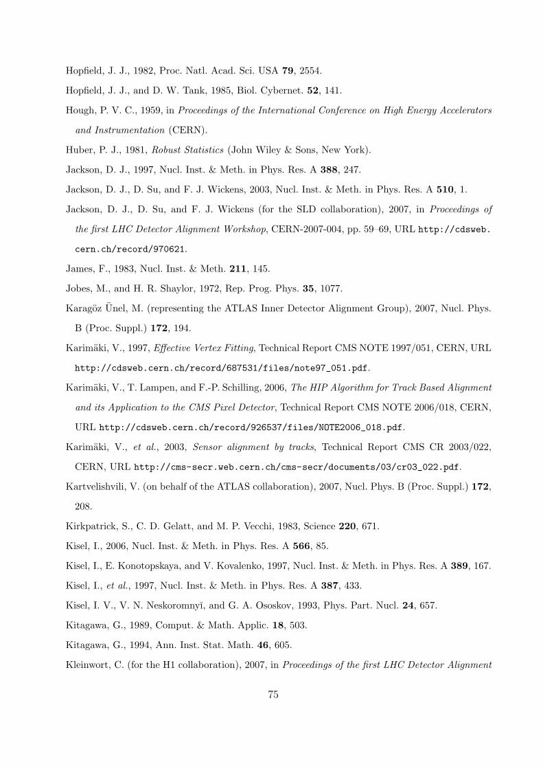
Hopfield, J. J., 1982, Proc. Natl. Acad. Sci. USA 79, 2554.

Hopfield, J. J., and D. W. Tank, 1985, Biol. Cybernet. 52, 141.

Hough, P. V. C., 1959, in Proceedings of the International Conference on High Energy Accelerators

and Instrumentation (CERN).

Huber, P. J., 1981, Robust Statistics (John Wiley & Sons, New York).

Jackson, D. J., 1997, Nucl. Inst. & Meth. in Phys. Res. A 388, 247.

Jackson, D. J., D. Su, and F. J. Wickens, 2003, Nucl. Inst. & Meth. in Phys. Res. A 510, 1.

Jackson, D. J., D. Su, and F. J. Wickens (for the SLD collaboration), 2007, in Proceedings of

the first LHC Detector Alignment Workshop, CERN-2007-004, pp. 59–69, URL http://cdsweb.

cern.ch/record/970621.

James, F., 1983, Nucl. Inst. & Meth. 211, 145.

Jobes, M., and H. R. Shaylor, 1972, Rep. Prog. Phys. 35, 1077.

Karagoz Unel, M. (representing the ATLAS Inner Detector Alignment Group), 2007, Nucl. Phys.

B (Proc. Suppl.) 172, 194.

Karimaki, V., 1997, Effective Vertex Fitting, Technical Report CMS NOTE 1997/051, CERN, URL

http://cdsweb.cern.ch/record/687531/files/note97_051.pdf.

Karimaki, V., T. Lampen, and F.-P. Schilling, 2006, The HIP Algorithm for Track Based Alignment

and its Application to the CMS Pixel Detector, Technical Report CMS NOTE 2006/018, CERN,

URL http://cdsweb.cern.ch/record/926537/files/NOTE2006_018.pdf.

Karimaki, V., et al., 2003, Sensor alignment by tracks, Technical Report CMS CR 2003/022,

CERN, URL http://cms-secr.web.cern.ch/cms-secr/documents/03/cr03_022.pdf.

Kartvelishvili, V. (on behalf of the ATLAS collaboration), 2007, Nucl. Phys. B (Proc. Suppl.) 172,

208.

Kirkpatrick, S., C. D. Gelatt, and M. P. Vecchi, 1983, Science 220, 671.

Kisel, I., 2006, Nucl. Inst. & Meth. in Phys. Res. A 566, 85.

Kisel, I., E. Konotopskaya, and V. Kovalenko, 1997, Nucl. Inst. & Meth. in Phys. Res. A 389, 167.

Kisel, I., et al., 1997, Nucl. Inst. & Meth. in Phys. Res. A 387, 433.

Kisel, I. V., V. N. Neskoromnyı, and G. A. Ososkov, 1993, Phys. Part. Nucl. 24, 657.

Kitagawa, G., 1989, Comput. & Math. Applic. 18, 503.

Kitagawa, G., 1994, Ann. Inst. Stat. Math. 46, 605.

Kleinwort, C. (for the H1 collaboration), 2007, in Proceedings of the first LHC Detector Alignment

75

Workshop, CERN-2007-004, pp. 41–49, URL http://cdsweb.cern.ch/record/970621.

Kohno, T., 2006, Nucl. Inst. & Meth. in Phys. Res. A 559, 153.

Kortner, O., et al., 2007, Nucl. Inst. & Meth. in Phys. Res. A 581, 545.

Kruskal, J. B., 1956, Proc. Amer. Math. Soc. 7, 48.

Lampen, T., et al., 2008, Comprehensive Set of Misalignment Scenarios for the CMS Tracker, Tech-

nical Report CMS NOTE-2008/029, CERN, URL http://cms.cern.ch/iCMS/jsp/openfile.

jsp?type=NOTE&year=2008&files=NOTE2008_029.pdf.

Laurikainen, P., W. G. Moorhead, and W. Matt, 1972, Nucl. Inst. & Meth. 98, 349.

Leo, W. R., 1994, Techniques for Nuclear and Particle Physics Experiments: A How-to Approach

(Springer, New York Berlin Heidelberg), 2nd edition.

Lin, D., and I. Guttman, 1993, Stat. Probabil. Lett. 16, 259.

Lindsey, C. S., and B. Denby, 1991, Nucl. Inst. & Meth. in Phys. Res. A 302, 217.

Lindstrom, M., 1995, Nucl. Inst. & Meth. in Phys. Res. A 357, 129.

Mankel, R., 1997, Nucl. Inst. & Meth. in Phys. Res. A 395, 169.

Mankel, R., 2004, Rep. Prog. Phys. 67, 553.

Mankel, R. (for the ZEUS collaboration), 2007, in Proceedings of the first LHC Detector Alignment

Workshop, CERN-2007-004, pp. 51–58, URL http://cdsweb.cern.ch/record/970621.

Margetis, S., et al. (for the STAR collaboration), 2007, in Proceedings of the first LHC Detec-

tor Alignment Workshop, CERN-2007-004, pp. 23–28, URL http://cdsweb.cern.ch/record/

970621.

Morley, A. (on behalf of the ATLAS Inner Detector Alignment Group), 2008, Nucl. Inst. & Meth.

in Phys. Res. A 596, 32.

Ohlsson, M., 1993, Comp. Phys. Comm. 77, 19.

Ohlsson, M., C. Peterson, and A. L. Yuille, 1992, Comp. Phys. Comm. 71, 77.

Peterson, C., 1989, Nucl. Inst. & Meth. in Phys. Res. A 279, 537.

Peterson, C., and J. R. Anderson, 1987, Complex Systems 1, 995.

Piacquadio, G., K. Prokofiev, and A. Wildauer, 2008, J. Phys.: Conf. Ser. 119, 032033, URL

http://dx.doi.org/10.1088/1742-6596/119/3/032033.

Regler, M., R. Fruhwirth, and W. Mitaroff, 1996, Int. J. Mod. Phys. C 7(4), 521.

Ronga, F. J. (for the CMS collaboration), 2007, Nucl. Phys. B (Proc. Suppl.) 172, 202.

Rousseeuw, P. J., and A. M. Leroy, 1987, Robust Regression and Outlier Detection (John Wiley &

76

Sons, New York).

Scandale, W., and F. Zimmermann, 2007, CERN Courier 47(2), 32.

Schleper, P., G. Steinbruck, and M. Stoye, 2008, J. Phys.: Conf. Ser. 119, 032040, URL http:

//dx.doi.org/10.1088/1742-6596/119/3/032040.

Second LHC Detector Alignment Workshop, 2007, URL http://indico.cern.ch/

conferenceOtherViews.py?view=standard&amp;confId=13681.

Sopczak, A. (on behalf of the DØ collaboration), 2006, Nucl. Inst. & Meth. in Phys. Res. A 566,

142.

Sopczak, A. (for the DØ collaboration), 2007, in Proceedings of the first LHC Detector Alignment

Workshop, CERN-2007-004, pp. 71–79, URL http://cdsweb.cern.ch/record/970621.

Speer, T., and R. Fruhwirth, 2006, Comp. Phys. Comm. 174, 935.

Speer, T., et al., 2006a, Nucl. Inst. & Meth. in Phys. Res. A 566, 149.

Speer, T., et al., 2006b, Nucl. Inst. & Meth. in Phys. Res. A 559, 143.

Speer, T., et al., 2006c, Vertex Fitting in the CMS Tracker, Technical Report CMS NOTE

2006/032, CERN, URL http://cdsweb.cern.ch/record/927395/files/NOTE2006_032.pdf.

Stepanov, N., and A. Khanov, 1997, Nucl. Inst. & Meth. in Phys. Res. A 389, 177.

Stimpfl-Abele, G., and L. Garrido, 1991, Comp. Phys. Comm. 64, 46.

Strandlie, A., 2000, Adaptive methods for the reconstruction of charged tracks in a noisy environ-

ment, Ph.D. thesis, University of Oslo.

Strandlie, A., and R. Fruhwirth, 2000, Comp. Phys. Comm. 133, 34.

Strandlie, A., and R. Fruhwirth, 2006a, IEEE Trans. Nucl. Sci. 53(6), 3842.

Strandlie, A., and R. Fruhwirth, 2006b, Nucl. Inst. & Meth. in Phys. Res. A 566, 157.

Strandlie, A., and W. Wittek, 2006, Nucl. Inst. & Meth. in Phys. Res. A 566, 687.

Strandlie, A., J. Wroldsen, R. Fruhwirth, and B. Lillekjendlie, 2000, Comp. Phys. Comm. 131, 95.

Strandlie, A., and J. Zerubia, 1999, Comp. Phys. Comm. 123, 77.

Third LHC Detector Alignment Workshop, 2009, URL http://indico.cern.ch/

conferenceOtherViews.py?view=standard&confId=50502.

Vanlaer, P., et al., 2006, Impact of CMS Silicon Tracker Misalignment on Track and Vertex Re-

construction, Technical Report CMS NOTE 2006/029, CERN, URL http://cdsweb.cern.ch/

record/927378/files/NOTE2006_029.pdf.

Viret, S. (on behalf of the LHCb VELO group), 2007, Nucl. Inst. & Meth. in Phys. Res. A 582,

77

806.

Viret, S., C. Parkes, and M. Gersabeck, 2008, Nucl. Inst. & Meth. in Phys. Res. A 596, 157.

Viret, S., C. Parles, and D. Petrie, 2005, LHCb VELO software alignment, Technical Report LHCb-

2005-101, CERN, URL http://cdsweb.cern.ch/record/914076/files/lhcb-2005-101.pdf.

Waltenberger, W., 2004, Development of Vertex Finding and Vertex Fitting Algorithms for CMS,

Ph.D. thesis, University of Technology, Vienna, URL http://publications.teilchen.at/

walten/ww_diss.pdf.

Waltenberger, W., 2008, Adaptive Vertex Reconstruction, Technical Report CMS NOTE-2008/033,

CERN, URL http://cms.cern.ch/iCMS/jsp/openfile.jsp?type=NOTE&year=2008&files=

NOTE2008_033.pdf.

Waltenberger, W., R. Fruhwirth, and P. Vanlaer, 2007a, J. Phys. G: Nucl. Part. Phys. 34, N343.

Waltenberger, W., W. Mitaroff, and F. Moser, 2007b, Nucl. Inst. & Meth. in Phys. Res. A 581,

549.

Waltenberger, W., and F. Moser, 2006, in 2006 IEEE Nuclear Science Symposium Confer-

ence Record (IEEE), volume 1, p. 104, URL http://ieeexplore.ieee.org/servlet/opac?

punumber=4143535.

Weber, M. (for the CMS collaboration), 2007, in Proceedings of the first LHC Detector Alignment

Workshop, CERN-2007-004, pp. 95–104, URL http://cdsweb.cern.ch/record/970621.

Wicke, D., 1998, A new algorithm for solving tracking ambiguities, Technical Report DELPHI

98-163 PROG 236 TRACK 92, CERN, URL http://delphiwww.cern.ch/pubxx/delnote/

public/98_163_prog_236_track_92.ps.gz.

Widl, E., and R. Fruhwirth, 2008, J. Phys.: Conf. Ser. 119, 032038, URL http://dx.doi.org/

10.1088/1742-6596/119/3/032038.

Widl, E., and R. Fruhwirth, 2009, Application of the Kalman Alignment Algorithm to the CMS

Tracker, Technical Report CMS CR-2009/171, CERN, URL http://cms.cern.ch/iCMS/jsp/

openfile.jsp?type=CR&year=2009&files=CR2009_171.pdf.

Widl, E., R. Fruhwirth, and W. Adam, 2006, A Kalman Filter for Track-based Alignment, Technical

Report CMS NOTE 2006/022, CERN, URL http://cdsweb.cern.ch/record/927376/files/

NOTE2006_022.pdf.

Wiedenmann, W. (ALEPH collaboration), 1992, Alignment of the ALEPH Tracking Devices, Tech-

nical Report CERN-PPE/92-90, CERN, URL http://doc.cern.ch/archive/electronic/

78

cern/preprints/ppe/ppe-92-090.pdf.

Wildauer, A., 2006, Primary Vertex Finding, b-Tagging and Analysis of the Channel ttH0, H0 −→

bb in the ATLAS Experiment, Ph.D. thesis, Leopold-Franzens-Universitat Innsbruck, URL http:

//physik.uibk.ac.at/hephy/theses/diss_aw.pdf.

Winkler, M., 2002, A comparative study of track reconstruction methods in the context of CMS

physics, Ph.D. thesis, University of Technology, Vienna, URL http://cdsweb.cern.ch/record/

583851/files/CM-P00040552.pdf.

Yuille, A., 1990, Neural Comput. 2, 1.

Yuille, A., P. Stolorz, and J. Utans, 1994, Neural Comput. 6, 334.

Zhao, H. W., 2000, Alignment of the Belle Silicon Vertex Detector with SVD Local Tracking at

B=0, Technical Report Belle-Note 348, KEK, URL http://osksn2.hep.sci.osaka-u.ac.jp/

~hara/Alignment/BelleNote348.ps.gz.

Figures

79

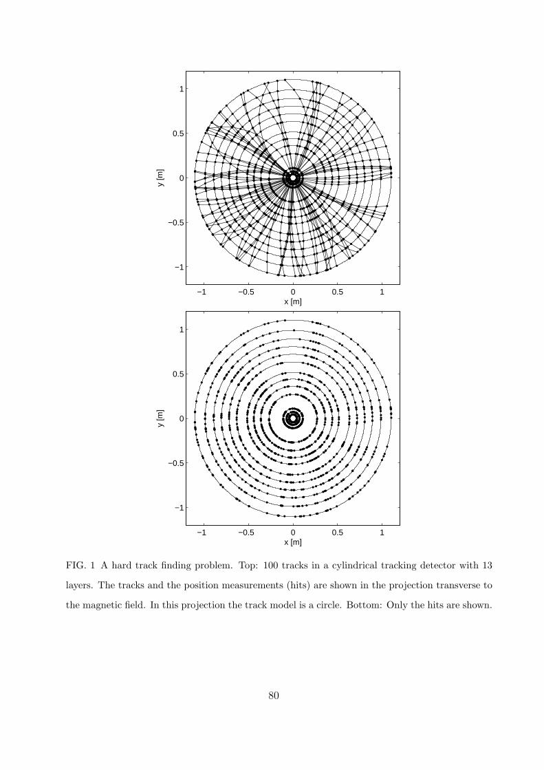
−1 −0.5 0 0.5 1

−1

−0.5

0

0.5

1

x [m]

y [m

]

−1 −0.5 0 0.5 1

−1

−0.5

0

0.5

1

x [m]

y [m

]

1

FIG. 1 A hard track finding problem. Top: 100 tracks in a cylindrical tracking detector with 13

layers. The tracks and the position measurements (hits) are shown in the projection transverse to

the magnetic field. In this projection the track model is a circle. Bottom: Only the hits are shown.

80

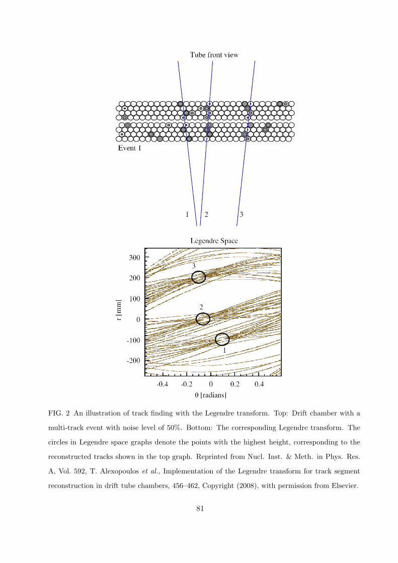
1

FIG. 2 An illustration of track finding with the Legendre transform. Top: Drift chamber with a

multi-track event with noise level of 50%. Bottom: The corresponding Legendre transform. The

circles in Legendre space graphs denote the points with the highest height, corresponding to the

reconstructed tracks shown in the top graph. Reprinted from Nucl. Inst. & Meth. in Phys. Res.

A, Vol. 592, T. Alexopoulos et al., Implementation of the Legendre transform for track segment

reconstruction in drift tube chambers, 456–462, Copyright (2008), with permission from Elsevier.

81

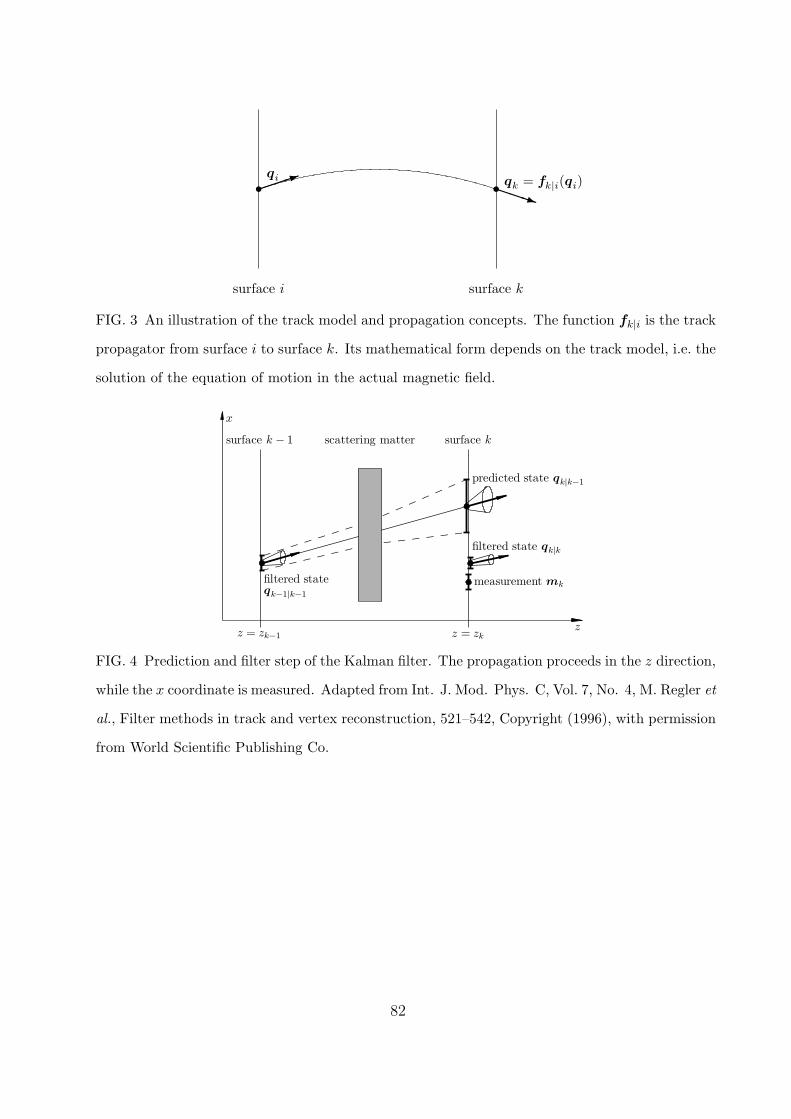
1 PPPqs sqi qk = fk|i(qi)

surface i surface k

FIG. 3 An illustration of the track model and propagation concepts. The function fk|i is the track

propagator from surface i to surface k. Its mathematical form depends on the track model, i.e. the

solution of the equation of motion in the actual magnetic field.

z

x

z = zk−1 z = zk

surface k − 1 surface k

filtered stateqk−1|k−1

scattering matter

predicted state qk|k−1

filtered state qk|k

measurement mk

FIG. 4 Prediction and filter step of the Kalman filter. The propagation proceeds in the z direction,

while the x coordinate is measured. Adapted from Int. J. Mod. Phys. C, Vol. 7, No. 4, M. Regler et

al., Filter methods in track and vertex reconstruction, 521–542, Copyright (1996), with permission

from World Scientific Publishing Co.

82

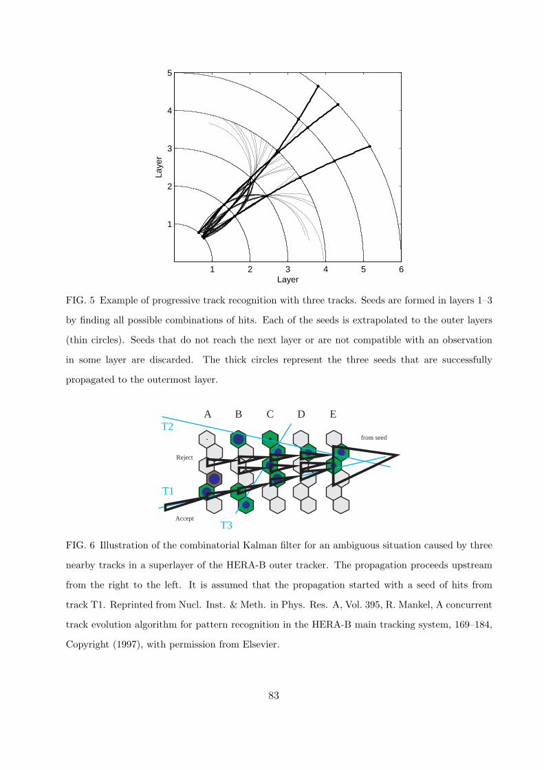
1 2 3 4 5 6

1

2

3

4

5

Layer

Laye

r

FIG. 5 Example of progressive track recognition with three tracks. Seeds are formed in layers 1–3

by finding all possible combinations of hits. Each of the seeds is extrapolated to the outer layers

(thin circles). Seeds that do not reach the next layer or are not compatible with an observation

in some layer are discarded. The thick circles represent the three seeds that are successfully

propagated to the outermost layer.

from seed

Reject

Accept

A B C D ET2

T1

T3

FIG. 6 Illustration of the combinatorial Kalman filter for an ambiguous situation caused by three

nearby tracks in a superlayer of the HERA-B outer tracker. The propagation proceeds upstream

from the right to the left. It is assumed that the propagation started with a seed of hits from

track T1. Reprinted from Nucl. Inst. & Meth. in Phys. Res. A, Vol. 395, R. Mankel, A concurrent

track evolution algorithm for pattern recognition in the HERA-B main tracking system, 169–184,

Copyright (1997), with permission from Elsevier.

83

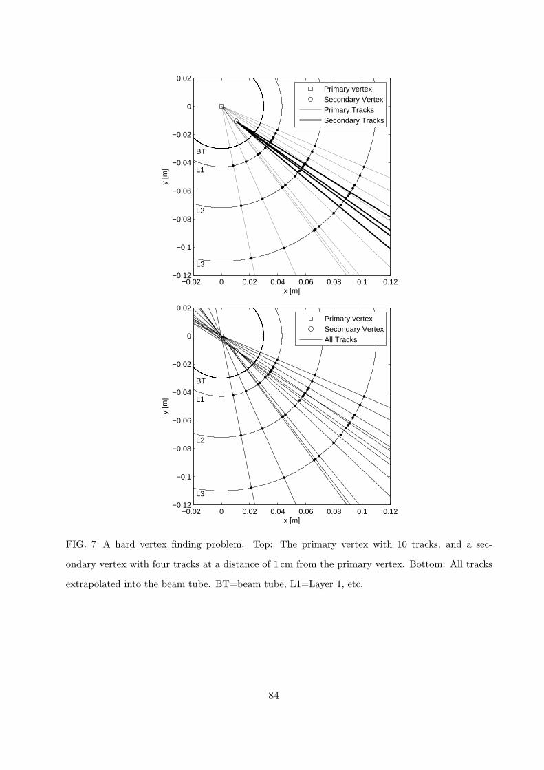
−0.02 0 0.02 0.04 0.06 0.08 0.1 0.12−0.12

−0.1

−0.08

−0.06

−0.04

−0.02

0

0.02

L1

L2

L3

BT

x [m]

y [m

]

Primary vertexSecondary VertexPrimary TracksSecondary Tracks

−0.02 0 0.02 0.04 0.06 0.08 0.1 0.12−0.12

−0.1

−0.08

−0.06

−0.04

−0.02

0

0.02

L1

L2

L3

BT

x [m]

y [m

]

Primary vertexSecondary VertexAll Tracks

1

FIG. 7 A hard vertex finding problem. Top: The primary vertex with 10 tracks, and a sec-

ondary vertex with four tracks at a distance of 1 cm from the primary vertex. Bottom: All tracks

extrapolated into the beam tube. BT=beam tube, L1=Layer 1, etc.

84

FIG. 8 The neural network architecture used to determine the vertex of tracks in 18-wire z-chamber

subsections. All input units and the bias unit are connected to all hidden units. All hidden units

and the bias unit are connected to all output units. Only a few of the connections are shown. The

bias unit has an output activation fixed to 1.0. Reprinted from Nucl. Inst. & Meth. in Phys. Res.

A, Vol. 302, C.S. Lindsey and B. Denby, Primary vertex finding in proton–antiproton events with

a neural network simulation, 217–226, Copyright (1991), with permission from Elsevier.

v

p1p2p3

p4 p5

q1q2q3

q4 q5

reference surfaceR = Rref

reference surfaceR = Rref

FIG. 9 Vertex parameters v (position), p1, . . . ,p5 (momentum vectors) and estimated track pa-

rameters q1, . . . , q5 for a vertex with five tracks. The reference surface is a cylinder with radius

R = Rref .

85

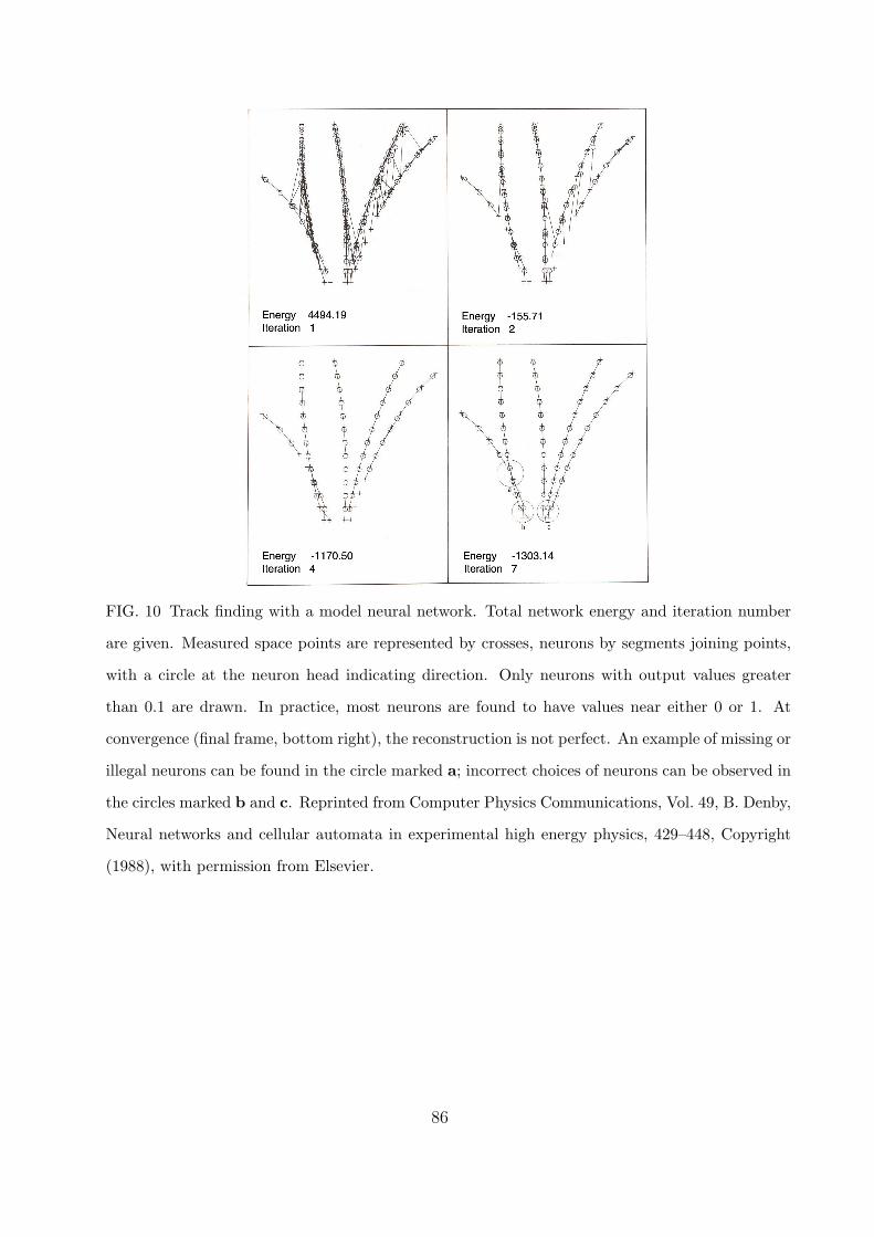
FIG. 10 Track finding with a model neural network. Total network energy and iteration number

are given. Measured space points are represented by crosses, neurons by segments joining points,

with a circle at the neuron head indicating direction. Only neurons with output values greater

than 0.1 are drawn. In practice, most neurons are found to have values near either 0 or 1. At

convergence (final frame, bottom right), the reconstruction is not perfect. An example of missing or

illegal neurons can be found in the circle marked a; incorrect choices of neurons can be observed in

the circles marked b and c. Reprinted from Computer Physics Communications, Vol. 49, B. Denby,

Neural networks and cellular automata in experimental high energy physics, 429–448, Copyright

(1988), with permission from Elsevier.

86

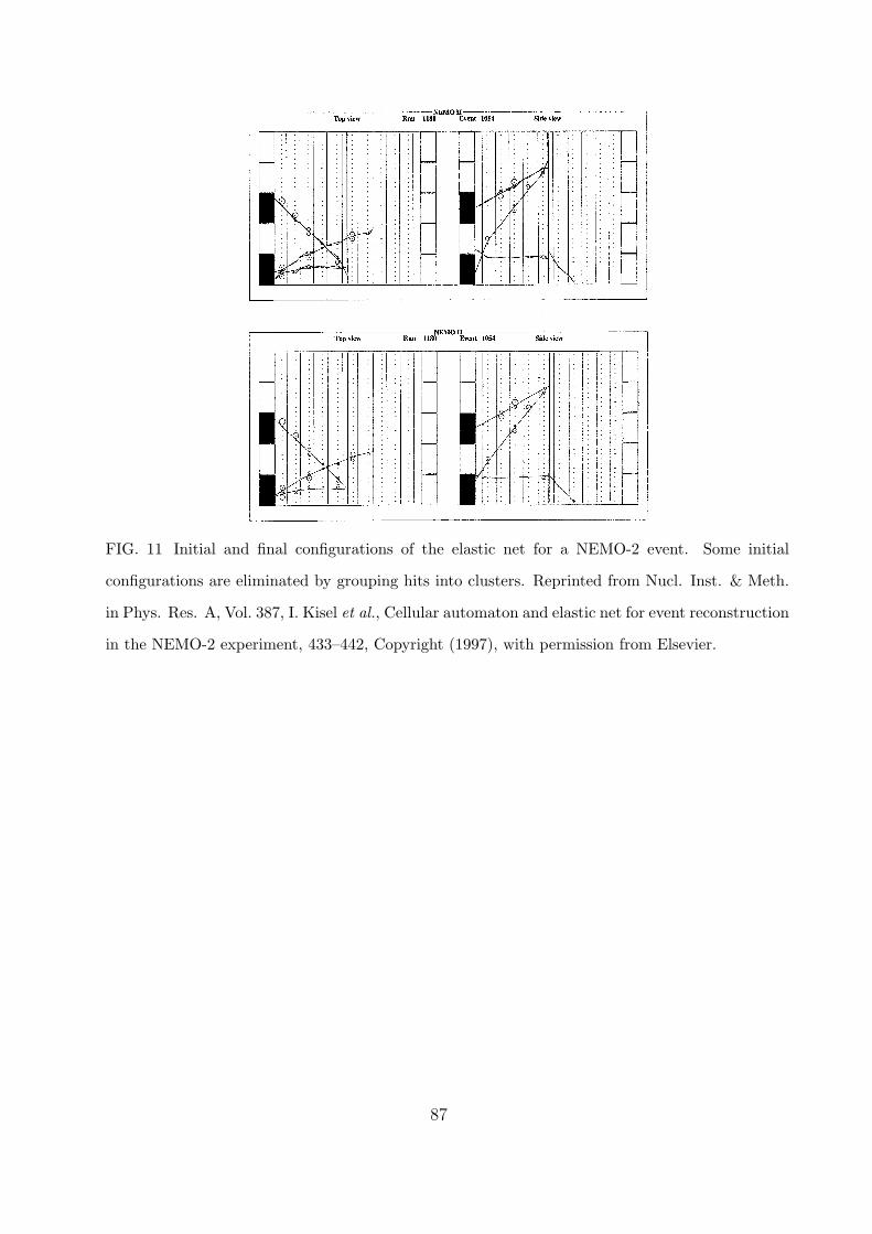
FIG. 11 Initial and final configurations of the elastic net for a NEMO-2 event. Some initial

configurations are eliminated by grouping hits into clusters. Reprinted from Nucl. Inst. & Meth.

in Phys. Res. A, Vol. 387, I. Kisel et al., Cellular automaton and elastic net for event reconstruction

in the NEMO-2 experiment, 433–442, Copyright (1997), with permission from Elsevier.

87

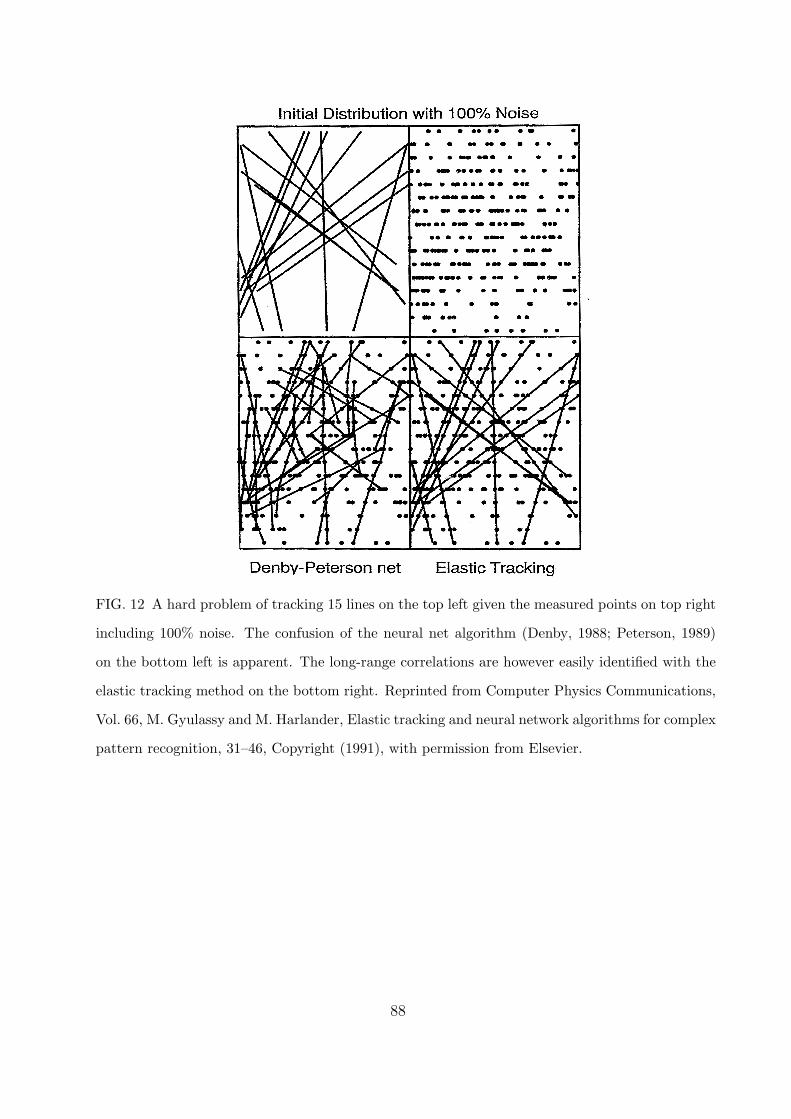
1

FIG. 12 A hard problem of tracking 15 lines on the top left given the measured points on top right

including 100% noise. The confusion of the neural net algorithm (Denby, 1988; Peterson, 1989)

on the bottom left is apparent. The long-range correlations are however easily identified with the

elastic tracking method on the bottom right. Reprinted from Computer Physics Communications,

Vol. 66, M. Gyulassy and M. Harlander, Elastic tracking and neural network algorithms for complex

pattern recognition, 31–46, Copyright (1991), with permission from Elsevier.

88

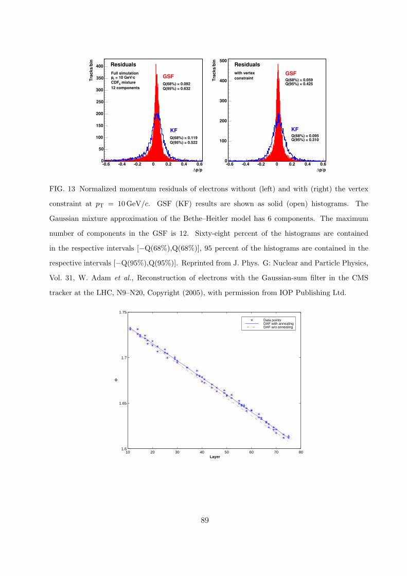
N18 Note

(q/p)σ(q/p)/ ∆-6 -4 -2 0 2 4 6

Tra

cks/

bin

0

200

400

600

800

1000

1200

1400

1600

GSF

KF

Pull quantities

Full simulation = 10 GeV/ctp

mixture6CDF12 components

Mean: 0.12RMS: 1.32

Mean: 0.06RMS: 1.25

Probability transform for q/p0 0.1 0.2 0.3 0.4 0.5 0.6 0.7 0.8 0.9 1

Fra

ctio

n o

f tr

acks

/bin

0

0.005

0.01

0.015

0.02

0.025

0.03

0.035

0.04

0.045KF

GSF

Figure 9. Left: pull quantities for q/p for the GSF (solid histogram) and the KF (open histogram).The values for mean and RMS shown in the figure were obtained using truncation at the histogramlimits. Right: distributions of the probability transform for q/p.

p/p∆-0.6 -0.4 -0.2 0 0.2 0.4 0.6

Tra

cks/

bin

0

50

100

150

200

250

300

350

400

KF

GSF

Residuals

Full simulation = 10 GeV/ctp

mixture6CDF12 components

Q(68%) = 0.092Q(95%) = 0.632

Q(68%) = 0.119Q(95%) = 0.522

p/ p∆-0.6 -0.4 -0.2 0 0.2 0.4 0.6

Tra

cks/

bin

0

100

200

300

400

500

GSF

KF

Residualswith vertexconstraint Q(68%) = 0.059

Q(95%) = 0.425

Q(68%) = 0.095Q(95%) = 0.310

Figure 10. Normalized momentum residuals without (left) and with (right) the vertex constraintat pt = 10 GeV/c. GSF (KF) results are shown as solid (open) histograms.

and azimuthal direction. This effect can be partially compensated by including a vertexconstraint—a procedure which will be used in many realistic applications. For this studythe prior knowledge on the distribution of generated vertices has been used, a conservativeassumption compared to the precision expected for the reconstruction of primary vertices inhigh energy proton–proton collisions. Figure 10 shows the distributions of the momentumresiduals with and without the vertex constraint for a CDF6-mixture and a pt of 10 GeV/c.Using the constraint renders distributions less skew, with modes closer to zero and a reductionof the population of tracks in the tails. The resolution, measured in terms of Q(68%), improvesby 35% for the GSF and 20% for the KF. This indicates the adaptive power of the GSF, whichwill select components based on the information contained in the vertex constraint.

FIG. 13 Normalized momentum residuals of electrons without (left) and with (right) the vertex

constraint at pT = 10 GeV/c. GSF (KF) results are shown as solid (open) histograms. The

Gaussian mixture approximation of the Bethe–Heitler model has 6 components. The maximum

number of components in the GSF is 12. Sixty-eight percent of the histograms are contained

in the respective intervals [−Q(68%),Q(68%)], 95 percent of the histograms are contained in the

respective intervals [−Q(95%),Q(95%)]. Reprinted from J. Phys. G: Nuclear and Particle Physics,

Vol. 31, W. Adam et al., Reconstruction of electrons with the Gaussian-sum filter in the CMS

tracker at the LHC, N9–N20, Copyright (2005), with permission from IOP Publishing Ltd.

10 20 30 40 50 60 70 801.6

1.65

1.7

1.75

Layer

Φ

Data pointsDAF with annealingDAF w/o annealing

89

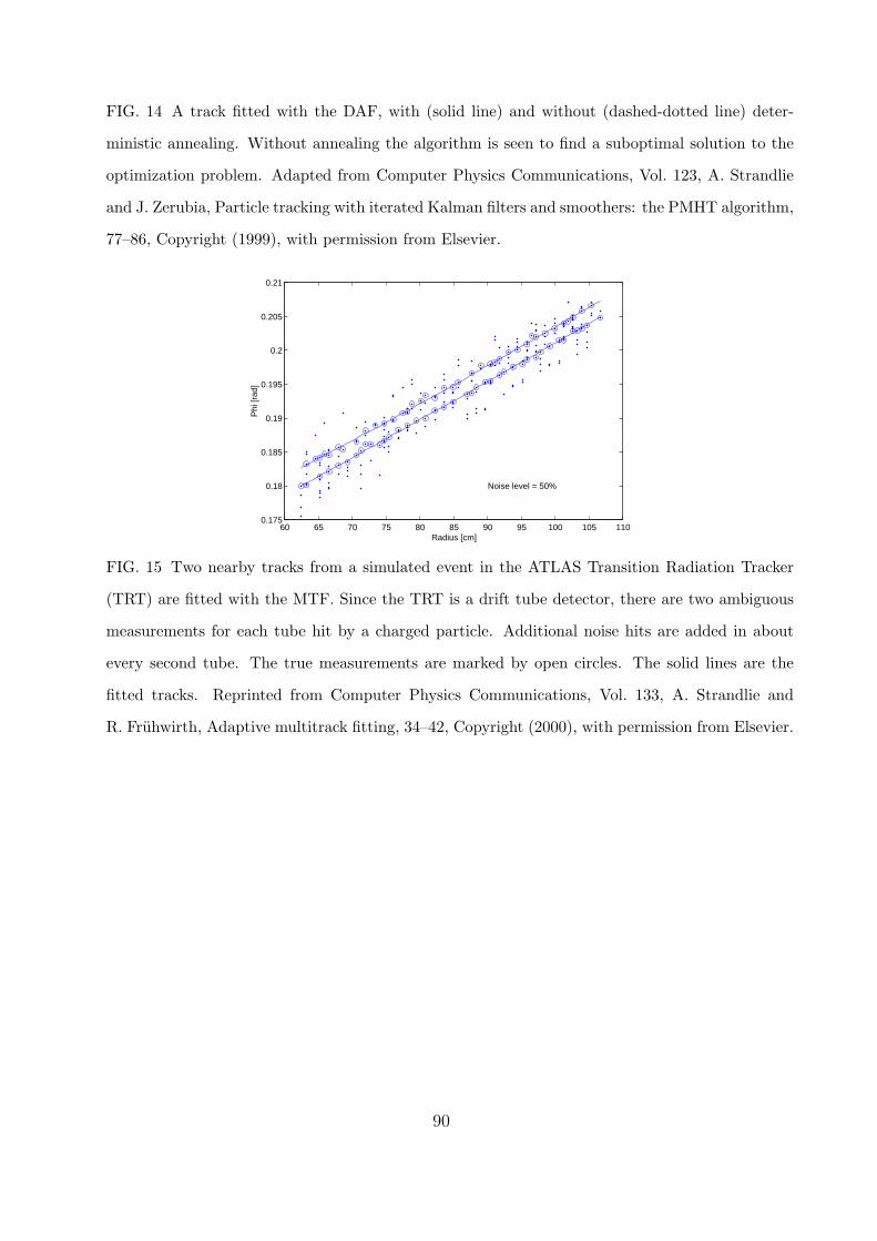
FIG. 14 A track fitted with the DAF, with (solid line) and without (dashed-dotted line) deter-

ministic annealing. Without annealing the algorithm is seen to find a suboptimal solution to the

optimization problem. Adapted from Computer Physics Communications, Vol. 123, A. Strandlie

and J. Zerubia, Particle tracking with iterated Kalman filters and smoothers: the PMHT algorithm,

77–86, Copyright (1999), with permission from Elsevier.

60 65 70 75 80 85 90 95 100 105 1100.175

0.18

0.185

0.19

0.195

0.2

0.205

0.21

Radius [cm]

Phi

[rad

]

Noise level = 50%

FIG. 15 Two nearby tracks from a simulated event in the ATLAS Transition Radiation Tracker

(TRT) are fitted with the MTF. Since the TRT is a drift tube detector, there are two ambiguous

measurements for each tube hit by a charged particle. Additional noise hits are added in about

every second tube. The true measurements are marked by open circles. The solid lines are the

fitted tracks. Reprinted from Computer Physics Communications, Vol. 133, A. Strandlie and

R. Fruhwirth, Adaptive multitrack fitting, 34–42, Copyright (2000), with permission from Elsevier.

90

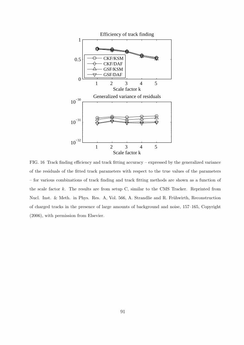
1 2 3 4 5 0

0.5

1Efficiency of track finding

Scale factor k

CKF/KSMCKF/DAFGSF/KSMGSF/DAF

1 2 3 4 5 10

−32

10−31

10−30

Generalized variance of residuals

Scale factor k

FIG. 16 Track finding efficiency and track fitting accuracy – expressed by the generalized variance

of the residuals of the fitted track parameters with respect to the true values of the parameters

– for various combinations of track finding and track fitting methods are shown as a function of

the scale factor k. The results are from setup C, similar to the CMS Tracker. Reprinted from

Nucl. Inst. & Meth. in Phys. Res. A, Vol. 566, A. Strandlie and R. Fruhwirth, Reconstruction

of charged tracks in the presence of large amounts of background and noise, 157–165, Copyright

(2006), with permission from Elsevier.

91

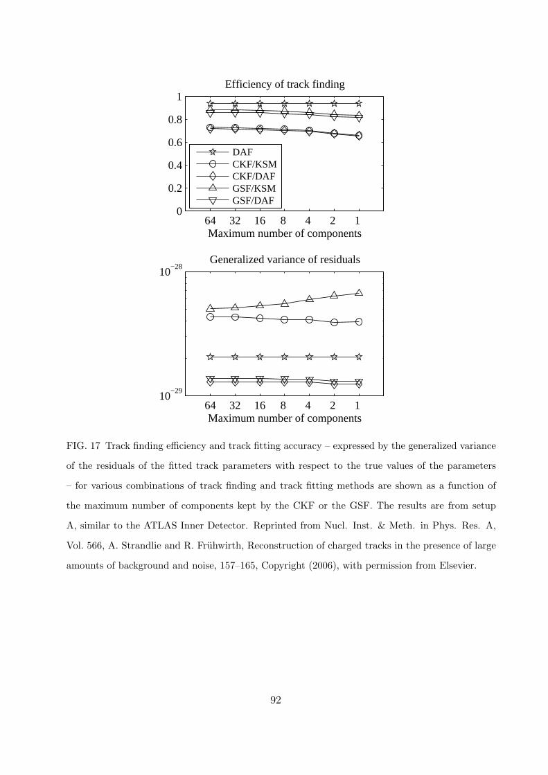
64 32 16 8 4 2 1 0

0.2

0.4

0.6

0.8

1Efficiency of track finding

Maximum number of components

DAFCKF/KSMCKF/DAFGSF/KSMGSF/DAF

64 32 16 8 4 2 1 10

−29

10−28

Generalized variance of residuals

Maximum number of components

FIG. 17 Track finding efficiency and track fitting accuracy – expressed by the generalized variance

of the residuals of the fitted track parameters with respect to the true values of the parameters

– for various combinations of track finding and track fitting methods are shown as a function of

the maximum number of components kept by the CKF or the GSF. The results are from setup

A, similar to the ATLAS Inner Detector. Reprinted from Nucl. Inst. & Meth. in Phys. Res. A,

Vol. 566, A. Strandlie and R. Fruhwirth, Reconstruction of charged tracks in the presence of large

amounts of background and noise, 157–165, Copyright (2006), with permission from Elsevier.

92

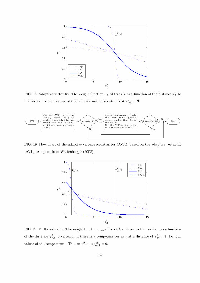
0 5 10 150

0.2

0.4

0.6

0.8

1

χ2cut

=9

χ2k

wk

T=9T=4T=1T=0.1

FIG. 18 Adaptive vertex fit. The weight function wk of track k as a function of the distance χ2k to

the vertex, for four values of the temperature. The cutoff is at χ2cut = 9.

AVR -

Use the AVF to fit theprimary vertex, using alltracks. Optionally take intoaccount the beam spot con-straint and known primarytracks.

-

QQQQ

QQQQ

Successful fit? -Yes

Select non-primary tracksthat have been assigned aweight smaller than 0.5 inthe last fit.Use the AVF to fit a vertexwith the selected tracks.

-

QQQQ

QQQQ

Successful fit? -No

End

No

6

Yes

6

FIG. 19 Flow chart of the adaptive vertex reconstructor (AVR), based on the adaptive vertex fit

(AVF). Adapted from Waltenberger (2008).

0 5 10 150

0.2

0.4

0.6

0.8

1

χ2cut

=9χ2ik

=1

χ2nk

wnk

T=9T=4T=1T=0.1

FIG. 20 Multi-vertex fit. The weight function wnk of track k with respect to vertex n as a function

of the distance χ2nk to vertex n, if there is a competing vertex i at a distance of χ2

ik = 1, for four

values of the temperature. The cutoff is at χ2cut = 9.

93

x

y

z

R

R

Φ

Φ

FIG. 21 A cylindrical detector and the coordinates R,Φ and z. The effects of distortions in these

three coordinates are described in Table V. For instance, a distortion ∆Φ that varies with z is a

twist.

94

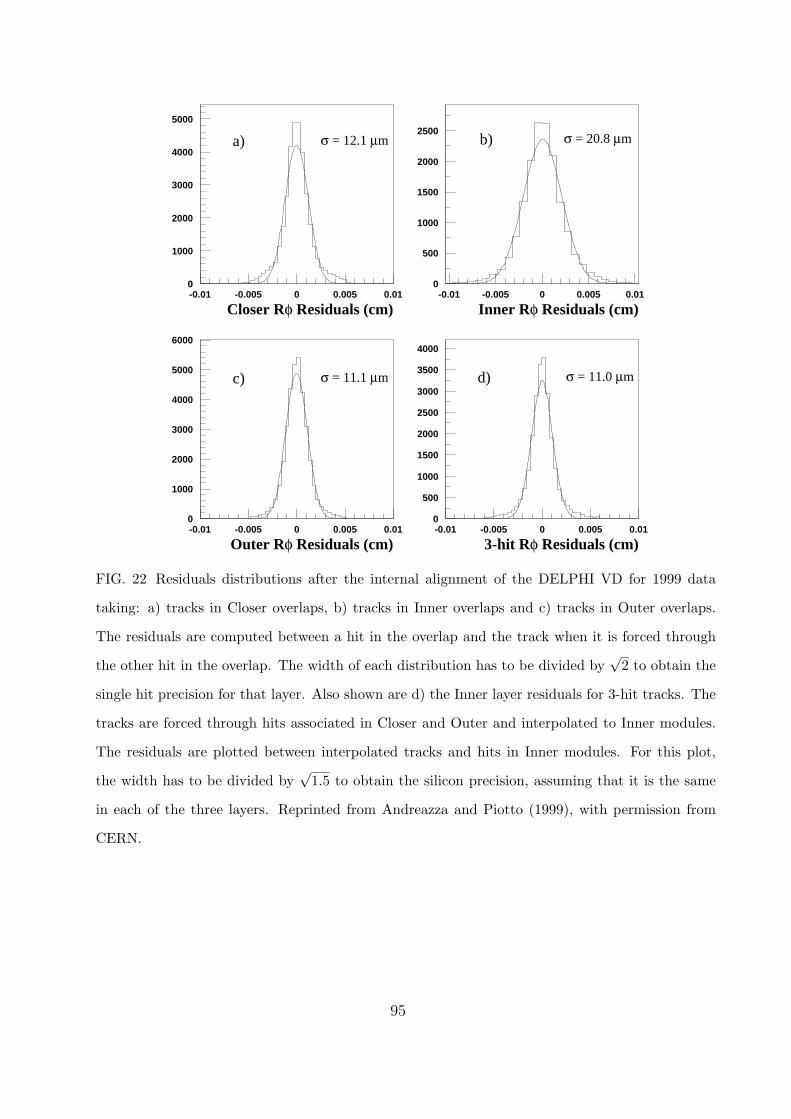
3 VD-OD alignment

3.1 The Rφ alignment

The Vertex Detector consists of 68 modules arranged in three layers (Closer, Inner, Outer).It must be internally aligned [1] before its overall position, considering the VD as a rigidobject, is found with respect to the other tracking detectors. The internal alignment isobtained assigning the status of master to a layer (until 1998 it was the Outer, in 1999 itwas the Closer), and treating the others layers (Inner and Closer till 1998, Inner and Outerin 1999) as slaves. This means that the Closer layer is aligned as a full pseudo-cylindricalobject using all Rφ and Z overlap constraints between adjacent modules. Modules of slavelayers are aligned individually with respect to the corresponding master modules. Theoverall quality of VD alignment is estimated comparing intrinsic hit precision (measuredfrom residuals of tracks in the overlaps in the master layer) with the effective hit precision(measured from the residuals of tracks in the overlaps in the slave layers and which havenot been used in the alignment procedure). This can be seen in figure 1.

DELPHI

0

1000

2000

3000

4000

5000

-0.01 -0.005 0 0.005 0.01

Closer Rφ Residuals (cm)

σ = 12.1 µma)

0

500

1000

1500

2000

2500

-0.01 -0.005 0 0.005 0.01

Inner Rφ Residuals (cm)

σ = 20.8 µmb)

0

1000

2000

3000

4000

5000

6000

-0.01 -0.005 0 0.005 0.01

Outer Rφ Residuals (cm)

σ = 11.1 µmc)

0

500

1000

1500

2000

2500

3000

3500

4000

-0.01 -0.005 0 0.005 0.01

3-hit Rφ Residuals (cm)

σ = 11.0 µmd)

Figure 1: Residuals distributions after internal alignment for 1999 data taking: a) tracksin Closer overlaps, b) tracks in Inner overlaps and c) tracks in Outer overlaps. Theresiduals are computed between an hit in the overlap and the track when it is forcedthrough the other hit in the overlap. The width of each distribution has to be dividedby√

2 to obtain the single hit precision for that layer. Also shown are d) the Inner layerresiduals for 3-hit tracks. The tracks are forced through hits associated in Closer andOuter and interpolated to Inner modules. The residuals are plotted between interpolatedtracks and hits in Inner. For this plot, the width has to be divided by

√1.5 to obtain the

silicon precision, assuming that it is the same in each of the three layers.

3

FIG. 22 Residuals distributions after the internal alignment of the DELPHI VD for 1999 data

taking: a) tracks in Closer overlaps, b) tracks in Inner overlaps and c) tracks in Outer overlaps.

The residuals are computed between a hit in the overlap and the track when it is forced through

the other hit in the overlap. The width of each distribution has to be divided by√

2 to obtain the

single hit precision for that layer. Also shown are d) the Inner layer residuals for 3-hit tracks. The

tracks are forced through hits associated in Closer and Outer and interpolated to Inner modules.

The residuals are plotted between interpolated tracks and hits in Inner modules. For this plot,

the width has to be divided by√

1.5 to obtain the silicon precision, assuming that it is the same

in each of the three layers. Reprinted from Andreazza and Piotto (1999), with permission from

CERN.

95

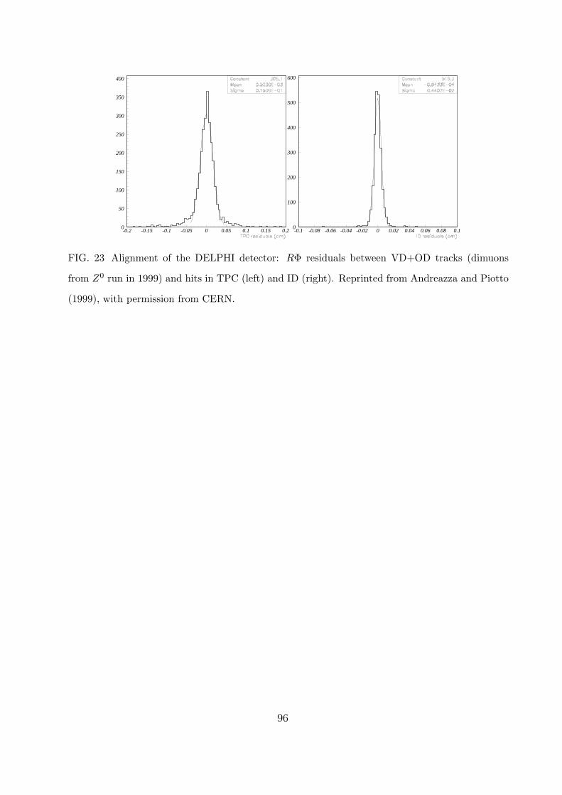
R1 R2 σ1 σ2 Rextr. σextr.

[cm] [cm] [µm] [µm] [cm] [µm]

VD only 6.3 10.9 9 9 RTPC =71 150VD + OD 6.3 201 9 120 RTPC =71 40VD only 6.3 10.9 9 9 RID =17.5 18

VD + OD 6.3 201 9 120 RID =17.5 10

Table 1: Resolution in µm obtained extrapolating tracks with VD hits only or with VDand OD hits. The extrapolation has been computed in the middle of TPC (Rextr.=71 cm)and in the middle of ID (Rextr.=17.5 cm).

0

50

100

150

200

250

300

350

400

-0.2 -0.15 -0.1 -0.05 0 0.05 0.1 0.15 0.20

100

200

300

400

500

600

-0.1 -0.08 -0.06 -0.04 -0.02 0 0.02 0.04 0.06 0.08 0.1

Figure 7: Rφ residuals between VD+OD tracks (dimuons from Z0 run in 1999) and hitsin TPC (left) and ID (right).

• the error on residuals (√

σ2point + σ2

extr.) is lower than in VD–OD;

• the number of useful tracks is greater because now each event is used twice (onceper track), and because it is possible to use events in which only one track has hitsin the OD;

• removing the collinearity hypothesis it is possible to reduce errors due to eventswith initial state radiation and to diverging beams.

5 Forward tracking detectors alignment

After having aligned the barrel detectors, the forward chambers (FC) are considered [3].First of all the Forward Chamber B (FCB) is taken in consideration. A sample of forwardmuons is selected and muon tracks are reconstructed using VD, VFT (Very ForwardTracker) and ID. In this case the TPC is not used even if it partially covers the angularregion of forward chambers, because of the distortions problem.

9

FIG. 23 Alignment of the DELPHI detector: RΦ residuals between VD+OD tracks (dimuons

from Z0 run in 1999) and hits in TPC (left) and ID (right). Reprinted from Andreazza and Piotto

(1999), with permission from CERN.

96

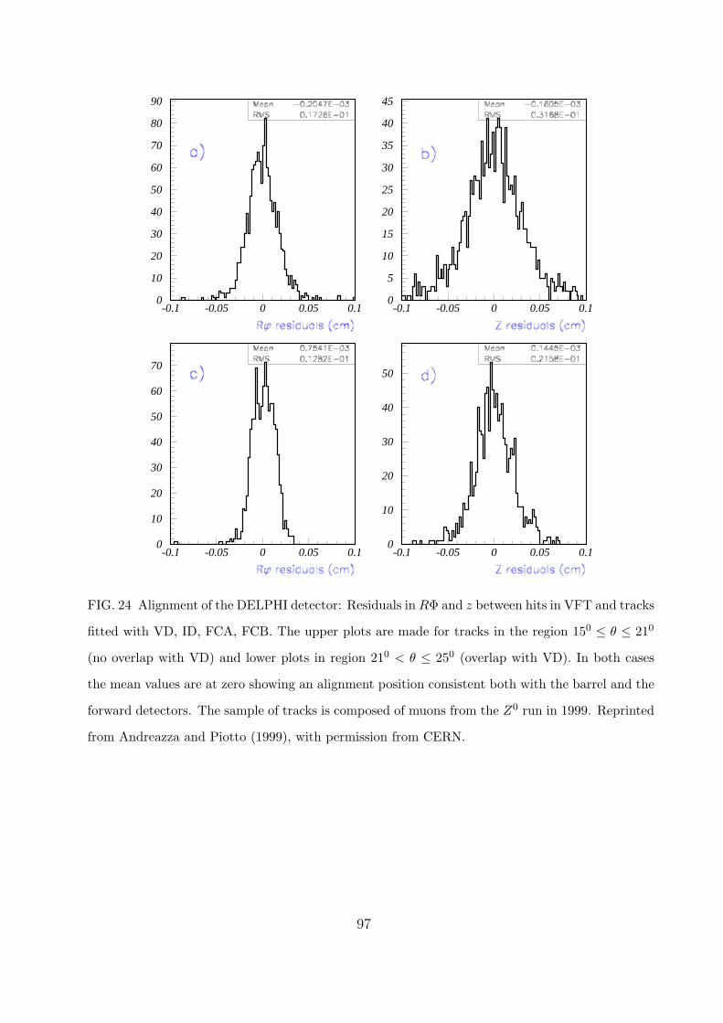
and ID reducing considerably the interpolation error to FCA. Sides A and C are treatedindependently.

The last step is the alignment of VFT [5]. Tracks fitted with VD, ID, FCA, FCBare used, and in this case also the information of beam spot is taken into consideration.All the degrees of freedom coming from considering the global position of VFT as a rigidobject and the ones coming from the internal positions of all modules are fixed minimisingresiduals from refitted tracks.

One should note that also in this case the TPC is not used. To assure a consistentposition of the VFT with respect to the other barrel detectors, the overlap between thefirst layer of pixels and the Outer layer of VD (in region 21o ≤ θ ≤ 25o) is used (see figure11).

0

10

20

30

40

50

60

70

80

90

-0.1 -0.05 0 0.05 0.10

5

10

15

20

25

30

35

40

45

-0.1 -0.05 0 0.05 0.1

0

10

20

30

40

50

60

70

-0.1 -0.05 0 0.05 0.10

10

20

30

40

50

-0.1 -0.05 0 0.05 0.1

Figure 11: Residuals in Rφ and Z between hits in VFT and tracks fitted with VD, ID,FCA, FCB. The upper plots are made for tracks in the region 15o ≤ θ ≤ 21o (no overlapwith VD) and lower plots in region 21o < θ < 25o (overlap with VD). In both cases themean values are at zero showing an alignment position consistent both with the barreland the forward detectors. The sample of tracks is composed by muons from Z0 run in1999.

6 Alignment with cosmics

The flux of cosmic rays through the DELPHI detector is not negligible. The study of thepotentiality of cosmic events in the alignment task is motivated by the lack of di-muonsfrom Z0 decays.

Some remarks are important when talking about cosmics:

12

FIG. 24 Alignment of the DELPHI detector: Residuals in RΦ and z between hits in VFT and tracks

fitted with VD, ID, FCA, FCB. The upper plots are made for tracks in the region 150 ≤ θ ≤ 210

(no overlap with VD) and lower plots in region 210 < θ ≤ 250 (overlap with VD). In both cases

the mean values are at zero showing an alignment position consistent both with the barrel and the

forward detectors. The sample of tracks is composed of muons from the Z0 run in 1999. Reprinted

from Andreazza and Piotto (1999), with permission from CERN.

97

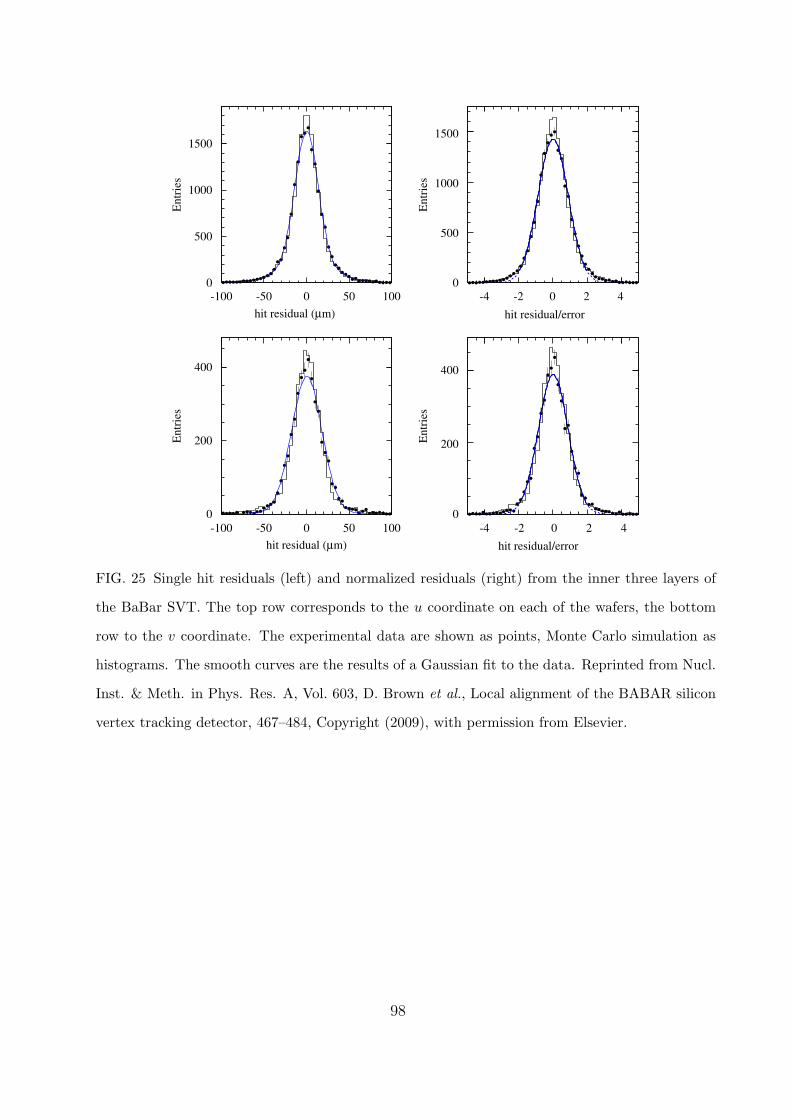
9. Validation of the alignment

We validate the performance of the SVT local alignmentprocedure through self-consistency tests using BABAR data, wherewe compare the results of the aligned detector with aprioriexpectations. We also compare the performance of the alignedBABAR detector with perfectly aligned Monte Carlo simulation. Thefollowing tests were performed using data from a typical period ofBABAR running, where the SVT alignment parameters weredetermined according to the procedure described above, applyingall the calibrations and corrections as normally done whenreconstructing BABAR data. The validation data sample hasminimal overlap with the data used for alignment production,due to the prescaling used in the alignment procedure.

We use the track residuals from SVT hits to perform a basic testof alignment self-consistency. The residuals themselves are shownin the plots on the left of Fig. 11, with the u residuals on top andthe v on the bottom. These show residuals from the inner threelayers of the SVT, using tracks in eþe ! mþm events selected tobe within 0.2 rad of vertical in the readout-view projection. Thisselection of hits gives the best resolution in the SVT, and soprovides the most sensitivity to misalignment. The residualdistributions are centered at zero, and the data and Monte Carlodistributions show very similar shapes. Both data and Monte Carlodistributions show some non-Gaussian tails, as expected fromscattering tails and hit resolution variation. The RMS of the dataand Monte Carlo distributions agree within a few percent. AGaussian fit to the core of the distributions gives mean valuesconsistent with zero, and sigma values of 14 ð13Þmm fordata (Monte Carlo) u hits, and 18 ð16Þmm for data (Monte Carlo)v hits, respectively. The data–Monte Carlo width differences are

consistent with the predicted accuracy of the simulation of SVT hitresolution.

The normalized residual (pull) distributions for the sametracks and hits are shown in the plots on the right of Fig. 11, withthe u residuals on top and the v on the bottom. Again we see goodagreement between data and Monte Carlo. The core of the datadistribution is well-described as a unit-width Gaussian centeredat 0. The non-Gaussian tails seen in both data and Monte Carlo areroughly consistent with known approximations in our estimate ofthe residual errors, which (for instance) do not take into accountdead electronics channels or Moliere scattering of the tracks.

A higher-level self-consistency test comes from fitting theincoming and outgoing branches of a cosmic ray as two separatetracks. Each of these tracks has a similar number of hits as atypical BABAR physics track. Both tracks are fit independently,butbecause they represent the same particle, they should haveequivalent parameters at the point where they meet if thealignment is correct. In this study we use cosmic ray eventsselected as described in Section 5. Fig. 12 compares the impactparameters and angles of the split cosmic tracks. These trackswere fit using their SVT hits plus a DCH curvature constraint,which reduces the large uncertainty in d0 and f coming from theircorrelation with curvature, which is poorly measured in the SVTalone due to its small lever arm. All tracks in these plots have amomentum above 2:0 GeV=c. The plots show good agreementbetween BABAR data and Monte Carlo. Fitting the BABAR datadistributions to a Gaussian we extract single-track resolutions of29mm for z0, 24mm for d0, 451mrad for f, and 512 106 fortanðp=2 yÞ, by scaling the fitted Gaussian sigma by 1=

ffiffiffi2p

.Another validation test comes from comparing the recon-

structed origin points of the two tracks produced in eþe ! mþm

ARTICLE IN PRESS

hit residual (μm)

-100

Ent

ries

0

500

1000

1500

hit residual/error

-4

Ent

ries

0

500

1000

1500

hit residual (μm)

-100

Ent

ries

0

200

400

hit residual/error

-4

Ent

ries

0

200

400

-50 500 100 -2 0 2 4

-50 50 100 -2 0 2 40

Fig. 11. Single hit residuals (left) and normalized residuals (right) in the u (top) and v (bottom) readout view. The BABAR data are shown as points, Monte Carlo simulation as

histograms. The (blue) smooth curves are the results of a Gaussian fit to the data. (For interpretation of the references to color in this figure legend, the reader is referred to

the web version of this article.)

D.N. Brown et al. / Nuclear Instruments and Methods in Physics Research A 603 (2009) 467–484478

FIG. 25 Single hit residuals (left) and normalized residuals (right) from the inner three layers of

the BaBar SVT. The top row corresponds to the u coordinate on each of the wafers, the bottom

row to the v coordinate. The experimental data are shown as points, Monte Carlo simulation as

histograms. The smooth curves are the results of a Gaussian fit to the data. Reprinted from Nucl.

Inst. & Meth. in Phys. Res. A, Vol. 603, D. Brown et al., Local alignment of the BABAR silicon

vertex tracking detector, 467–484, Copyright (2009), with permission from Elsevier.

98

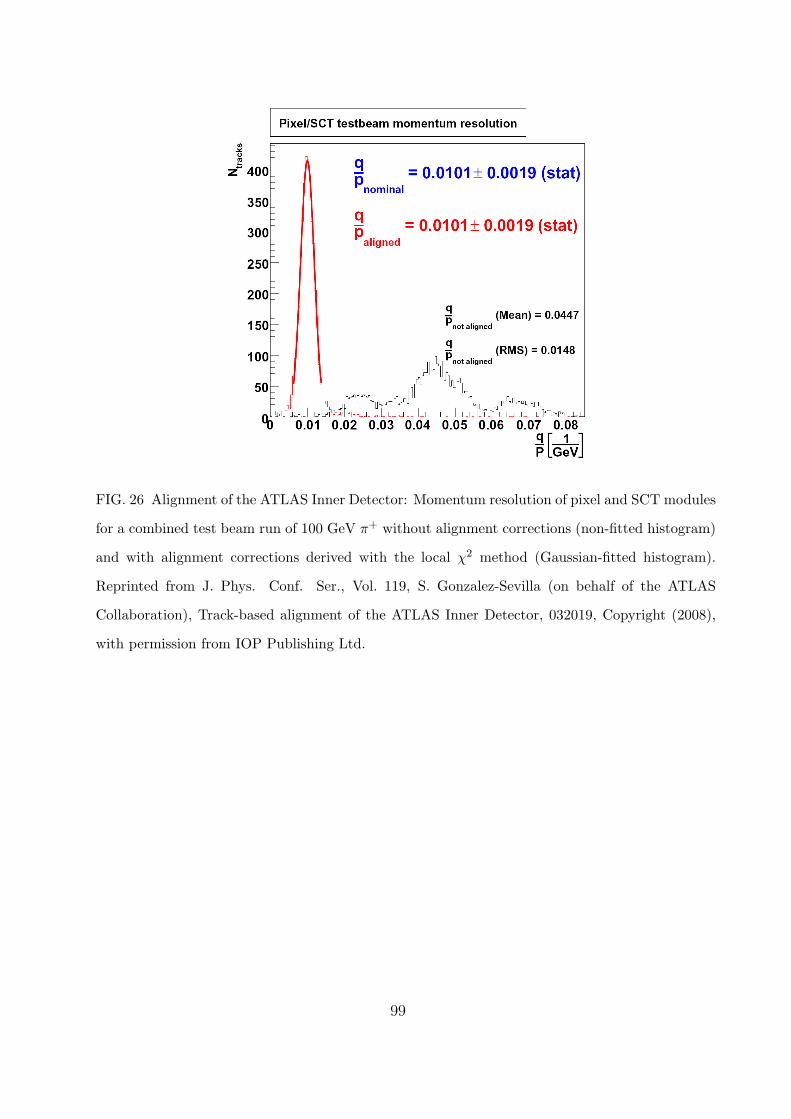
FIG. 26 Alignment of the ATLAS Inner Detector: Momentum resolution of pixel and SCT modules

for a combined test beam run of 100 GeV π+ without alignment corrections (non-fitted histogram)

and with alignment corrections derived with the local χ2 method (Gaussian-fitted histogram).

Reprinted from J. Phys. Conf. Ser., Vol. 119, S. Gonzalez-Sevilla (on behalf of the ATLAS

Collaboration), Track-based alignment of the ATLAS Inner Detector, 032019, Copyright (2008),

with permission from IOP Publishing Ltd.

99

[cm]x’

res-0.3 -0.2 -0.1 0 0.1 0.2 0.3

# h

its

0

1000

2000

3000

4000

5000

6000

RMS = 0.0498

= -0.0029! HIP

RMS = 0.0639

= 0.0029!

Millepede

RMS = 0.0461

= -0.0033!

Kalman

TIB

[cm]x’

res-0.3 -0.2 -0.1 0 0.1 0.2 0.3

# h

its

0

2000

4000

6000

8000

10000

12000

14000

16000

18000

20000

22000

RMS = 0.0367

= 0.0003! HIP

RMS = 0.0408

= -0.0006!

Millepede

RMS = 0.0314

= 0.0013!

Kalman

[cm]y’

res-3 -2 -1 0 1 2 3

# h

its

0

2000

4000

6000

8000

10000RMS = 0.4655

= 0.0089! HIP

RMS = 0.4769

= -0.0024!

Millepede

RMS = 0.4686

= -0.0140!

Kalman

[cm]x’

res-0.3 -0.2 -0.1 0 0.1 0.2 0.3

# h

its

0

5000

10000

15000

20000

25000

RMS = 0.0273

= -0.0009! HIP

RMS = 0.0284

= 0.0002!

Millepede

RMS = 0.0266

= -0.0005!

Kalman

TOB

[cm]x’

res-0.3 -0.2 -0.1 0 0.1 0.2 0.3

# h

its

0

10000

20000

30000

40000

50000RMS = 0.0288

= 0.0002! HIP

RMS = 0.0279

= 0.0002!

Millepede

RMS = 0.0278

= -0.0000!

Kalman

[cm]y’

res-3 -2 -1 0 1 2 3

# h

its

0

2000

4000

6000

8000

10000

12000

14000

RMS = 0.4539

= -0.0049! HIP

RMS = 0.5118

= -0.0076!

Millepede

RMS = 0.4581

= -0.0060!

Kalman

[cm]!r

res-0.3 -0.2 -0.1 0 0.1 0.2 0.3

# h

its

0

100

200

300

400

500

600

RMS = 0.0711

= 0.0061! HIP

RMS = 0.0719

= 0.0057!

Millepede

RMS = 0.0723

= 0.0050!

Kalman

TEC

[cm]!r

res-0.3 -0.2 -0.1 0 0.1 0.2 0.3

# h

its

0

200

400

600

800

1000

RMS = 0.0648

= 0.0016! HIP

RMS = 0.0661

= 0.0005!

Millepede

RMS = 0.0676

= 0.0008!

Kalman

[cm]r

res-3 -2 -1 0 1 2 3

# h

its

0

100

200

300

400

500

600

700

RMS = 0.6862

= -0.0332! HIP

RMS = 0.6963

= -0.0410!

Millepede

RMS = 0.6937

= -0.0408!

Kalman

TIB 1D

Modules

TIB 2D

Modules

TIB 2D

Modules

TOB 1D

Modules

TOB 2D

Modules

TOB 2D

Modules

[cm]x’

res-0.3 -0.2 -0.1 0 0.1 0.2 0.3

# h

its

0

1000

2000

3000

4000

5000

6000

RMS = 0.0498

= -0.0029! HIP

RMS = 0.0639

= 0.0029!

Millepede

RMS = 0.0461

= -0.0033!

Kalman

TIB

[cm]x’

res-0.3 -0.2 -0.1 0 0.1 0.2 0.3

# h

its

0

2000

4000

6000

8000

10000

12000

14000

16000

18000

20000

22000

RMS = 0.0367

= 0.0003! HIP

RMS = 0.0408

= -0.0006!

Millepede

RMS = 0.0314

= 0.0013!

Kalman

[cm]y’

res-3 -2 -1 0 1 2 3

# h

its

0

2000

4000

6000

8000

10000RMS = 0.4655

= 0.0089! HIP

RMS = 0.4769

= -0.0024!

Millepede

RMS = 0.4686

= -0.0140!

Kalman

[cm]x’

res-0.3 -0.2 -0.1 0 0.1 0.2 0.3

# h

its

0

5000

10000

15000

20000

25000

RMS = 0.0273

= -0.0009! HIP

RMS = 0.0284

= 0.0002!

Millepede

RMS = 0.0266

= -0.0005!

Kalman

TOB

[cm]x’

res-0.3 -0.2 -0.1 0 0.1 0.2 0.3

# h

its

0

10000

20000

30000

40000

50000RMS = 0.0288

= 0.0002! HIP

RMS = 0.0279

= 0.0002!

Millepede

RMS = 0.0278

= -0.0000!

Kalman

[cm]y’

res-3 -2 -1 0 1 2 3

# h

its

0

2000

4000

6000

8000

10000

12000

14000

RMS = 0.4539

= -0.0049! HIP

RMS = 0.5118

= -0.0076!

Millepede

RMS = 0.4581

= -0.0060!

Kalman

[cm]!r

res-0.3 -0.2 -0.1 0 0.1 0.2 0.3

# h

its

0

100

200

300

400

500

600

RMS = 0.0711

= 0.0061! HIP

RMS = 0.0719

= 0.0057!

Millepede

RMS = 0.0723

= 0.0050!

Kalman

TEC

[cm]!r

res-0.3 -0.2 -0.1 0 0.1 0.2 0.3

# h

its

0

200

400

600

800

1000

RMS = 0.0648

= 0.0016! HIP

RMS = 0.0661

= 0.0005!

Millepede

RMS = 0.0676

= 0.0008!

Kalman

[cm]r

res-3 -2 -1 0 1 2 3

# h

its

0

100

200

300

400

500

600

700

RMS = 0.6862

= -0.0332! HIP

RMS = 0.6963

= -0.0410!

Millepede

RMS = 0.6937

= -0.0408!

Kalman

TIB 1D

Modules

TIB 2D

Modules

TIB 2D

Modules

TOB 1D

Modules

TOB 2D

Modules

TOB 2D

Modules

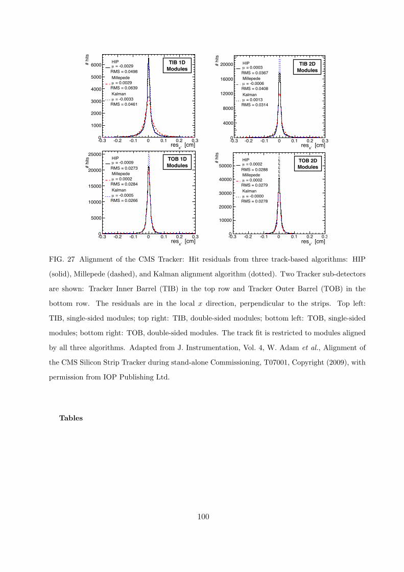
[cm]x’

res-0.3 -0.2 -0.1 0 0.1 0.2 0.3

# h

its

0

1000

2000

3000

4000

5000

6000

RMS = 0.0498

= -0.0029! HIP

RMS = 0.0639

= 0.0029!

Millepede

RMS = 0.0461

= -0.0033!

Kalman

TIB

[cm]x’

res-0.3 -0.2 -0.1 0 0.1 0.2 0.3

# h

its

0

2000

4000

6000

8000

10000

12000

14000

16000

18000

20000

22000

RMS = 0.0367

= 0.0003! HIP

RMS = 0.0408

= -0.0006!

Millepede

RMS = 0.0314

= 0.0013!

Kalman

[cm]y’

res-3 -2 -1 0 1 2 3

# h

its

0

2000

4000

6000

8000

10000RMS = 0.4655

= 0.0089! HIP

RMS = 0.4769

= -0.0024!

Millepede

RMS = 0.4686

= -0.0140!

Kalman

[cm]x’

res-0.3 -0.2 -0.1 0 0.1 0.2 0.3

# h

its

0

5000

10000

15000

20000

25000

RMS = 0.0273

= -0.0009! HIP

RMS = 0.0284

= 0.0002!

Millepede

RMS = 0.0266

= -0.0005!

Kalman

TOB

[cm]x’

res-0.3 -0.2 -0.1 0 0.1 0.2 0.3

# h

its

0

10000

20000

30000

40000

50000RMS = 0.0288

= 0.0002! HIP

RMS = 0.0279

= 0.0002!

Millepede

RMS = 0.0278

= -0.0000!

Kalman

[cm]y’

res-3 -2 -1 0 1 2 3

# h

its

0

2000

4000

6000

8000

10000

12000

14000

RMS = 0.4539

= -0.0049! HIP

RMS = 0.5118

= -0.0076!

Millepede

RMS = 0.4581

= -0.0060!

Kalman

[cm]!r

res-0.3 -0.2 -0.1 0 0.1 0.2 0.3

# h

its

0

100

200

300

400

500

600

RMS = 0.0711

= 0.0061! HIP

RMS = 0.0719

= 0.0057!

Millepede

RMS = 0.0723

= 0.0050!

Kalman

TEC

[cm]!r

res-0.3 -0.2 -0.1 0 0.1 0.2 0.3

# h

its

0

200

400

600

800

1000

RMS = 0.0648

= 0.0016! HIP

RMS = 0.0661

= 0.0005!

Millepede

RMS = 0.0676

= 0.0008!

Kalman

[cm]r

res-3 -2 -1 0 1 2 3

# h

its

0

100

200

300

400

500

600

700

RMS = 0.6862

= -0.0332! HIP

RMS = 0.6963

= -0.0410!

Millepede

RMS = 0.6937

= -0.0408!

Kalman

TIB 1D

Modules

TIB 2D

Modules

TIB 2D

Modules

TOB 1D

Modules

TOB 2D

Modules

TOB 2D

Modules

[cm]x’

res-0.3 -0.2 -0.1 0 0.1 0.2 0.3

# h

its

0

1000

2000

3000

4000

5000

6000

RMS = 0.0498

= -0.0029! HIP

RMS = 0.0639

= 0.0029!

Millepede

RMS = 0.0461

= -0.0033!

Kalman

TIB

[cm]x’

res-0.3 -0.2 -0.1 0 0.1 0.2 0.3

# h

its

0

2000

4000

6000

8000

10000

12000

14000

16000

18000

20000

22000

RMS = 0.0367

= 0.0003! HIP

RMS = 0.0408

= -0.0006!

Millepede

RMS = 0.0314

= 0.0013!

Kalman

[cm]y’

res-3 -2 -1 0 1 2 3

# h

its

0

2000

4000

6000

8000

10000RMS = 0.4655

= 0.0089! HIP

RMS = 0.4769

= -0.0024!

Millepede

RMS = 0.4686

= -0.0140!

Kalman

[cm]x’

res-0.3 -0.2 -0.1 0 0.1 0.2 0.3

# h

its

0

5000

10000

15000

20000

25000

RMS = 0.0273

= -0.0009! HIP

RMS = 0.0284

= 0.0002!

Millepede

RMS = 0.0266

= -0.0005!

Kalman

TOB

[cm]x’

res-0.3 -0.2 -0.1 0 0.1 0.2 0.3

# h

its

0

10000

20000

30000

40000

50000RMS = 0.0288

= 0.0002! HIP

RMS = 0.0279

= 0.0002!

Millepede

RMS = 0.0278

= -0.0000!

Kalman

[cm]y’

res-3 -2 -1 0 1 2 3

# h

its

0

2000

4000

6000

8000

10000

12000

14000

RMS = 0.4539

= -0.0049! HIP

RMS = 0.5118

= -0.0076!

Millepede

RMS = 0.4581

= -0.0060!

Kalman

[cm]!r

res-0.3 -0.2 -0.1 0 0.1 0.2 0.3

# h

its

0

100

200

300

400

500

600

RMS = 0.0711

= 0.0061! HIP

RMS = 0.0719

= 0.0057!

Millepede

RMS = 0.0723

= 0.0050!

Kalman

TEC

[cm]!r

res-0.3 -0.2 -0.1 0 0.1 0.2 0.3

# h

its

0

200

400

600

800

1000

RMS = 0.0648

= 0.0016! HIP

RMS = 0.0661

= 0.0005!

Millepede

RMS = 0.0676

= 0.0008!

Kalman

[cm]r

res-3 -2 -1 0 1 2 3

# h

its

0

100

200

300

400

500

600

700

RMS = 0.6862

= -0.0332! HIP

RMS = 0.6963

= -0.0410!

Millepede

RMS = 0.6937

= -0.0408!

Kalman

TIB 1D

Modules

TIB 2D

Modules

TIB 2D

Modules

TOB 1D

Modules

TOB 2D

Modules

TOB 2D

Modules

FIG. 27 Alignment of the CMS Tracker: Hit residuals from three track-based algorithms: HIP

(solid), Millepede (dashed), and Kalman alignment algorithm (dotted). Two Tracker sub-detectors

are shown: Tracker Inner Barrel (TIB) in the top row and Tracker Outer Barrel (TOB) in the

bottom row. The residuals are in the local x direction, perpendicular to the strips. Top left:

TIB, single-sided modules; top right: TIB, double-sided modules; bottom left: TOB, single-sided

modules; bottom right: TOB, double-sided modules. The track fit is restricted to modules aligned

by all three algorithms. Adapted from J. Instrumentation, Vol. 4, W. Adam et al., Alignment of

the CMS Silicon Strip Tracker during stand-alone Commissioning, T07001, Copyright (2009), with

permission from IOP Publishing Ltd.

Tables

100

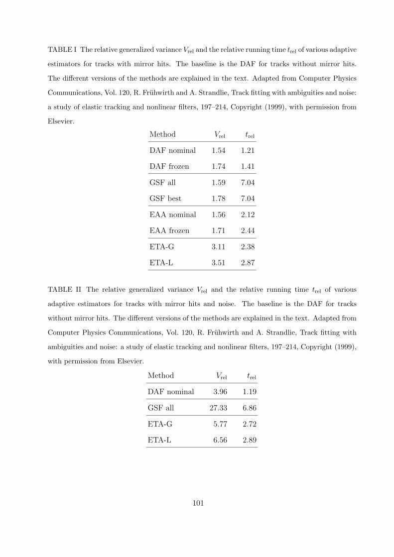
TABLE I The relative generalized variance Vrel and the relative running time trel of various adaptive

estimators for tracks with mirror hits. The baseline is the DAF for tracks without mirror hits.

The different versions of the methods are explained in the text. Adapted from Computer Physics

Communications, Vol. 120, R. Fruhwirth and A. Strandlie, Track fitting with ambiguities and noise:

a study of elastic tracking and nonlinear filters, 197–214, Copyright (1999), with permission from

Elsevier.

Method Vrel trel

DAF nominal 1.54 1.21

DAF frozen 1.74 1.41

GSF all 1.59 7.04

GSF best 1.78 7.04

EAA nominal 1.56 2.12

EAA frozen 1.71 2.44

ETA-G 3.11 2.38

ETA-L 3.51 2.87

TABLE II The relative generalized variance Vrel and the relative running time trel of various

adaptive estimators for tracks with mirror hits and noise. The baseline is the DAF for tracks

without mirror hits. The different versions of the methods are explained in the text. Adapted from

Computer Physics Communications, Vol. 120, R. Fruhwirth and A. Strandlie, Track fitting with

ambiguities and noise: a study of elastic tracking and nonlinear filters, 197–214, Copyright (1999),

with permission from Elsevier.

Method Vrel trel

DAF nominal 3.96 1.19

GSF all 27.33 6.86

ETA-G 5.77 2.72

ETA-L 6.56 2.89

101

TABLE III The relative generalized variance of the Multi-Track Fit with competition schemes 1–4,

at various noise levels with mirror hits. The baseline is a single-track fit of all tracks separately.

Reprinted from Computer Physics Communications, Vol. 133, A. Strandlie and R. Fruhwirth,

Adaptive multitrack fitting, 34–42, Copyright (2000), with permission from Elsevier.

Noise Competition scheme

level 1 2 3 4

0% 281 36.2 4.52 2.84

10% 270 58.7 5.35 4.35

20% 388 100.9 6.26 7.06

30% 358 185.3 7.19 9.51

40% 409 238.9 9.50 12.44

50% 653 301.6 11.66 17.65

TABLE IV Comparison of the main properties of the Kalman filter (KF) and the adaptive vertex

fit (AVF) on two physics processes. Top: Bs −→ J/ψφ −→ µ+µ−K+K−. Bottom: pp −→ ttH.

Reprinted from Nucl. Inst. & Meth. in Phys. Res. A, Vol. 566, T.Speer et al., Robust vertex

fitters, 149–152, Copyright (2006), with permission from Elsevier.

102

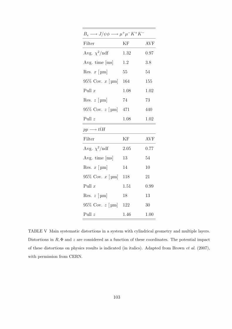
Bs −→ J/ψφ −→ µ+µ−K+K−

Filter KF AVF

Avg. χ2/ndf 1.32 0.97

Avg. time [ms] 1.2 3.8

Res. x [ µm] 55 54

95% Cov. x [ µm] 164 155

Pull x 1.08 1.02

Res. z [ µm] 74 73

95% Cov. z [ µm] 471 440

Pull z 1.08 1.02

pp −→ ttH

Filter KF AVF

Avg. χ2/ndf 2.05 0.77

Avg. time [ms] 13 54

Res. x [ µm] 14 10

95% Cov. x [ µm] 118 21

Pull x 1.51 0.99

Res. z [ µm] 18 13

95% Cov. z [ µm] 122 30

Pull z 1.46 1.00

TABLE V Main systematic distortions in a system with cylindrical geometry and multiple layers.

Distortions in R,Φ and z are considered as a function of these coordinates. The potential impact

of these distortions on physics results is indicated (in italics). Adapted from Brown et al. (2007),

with permission from CERN.

103

∆R ∆Φ ∆z

vs. Radial expansion Curl Telescope

R Distance scale Charge asymmetry z momentum

vs. Elliptical Clamshell Skew

Φ Vertex mass Vertex displacement z momentum

vs. Bowing Twist z expansion

z Total momentum CP violation Distance scale

104