Tracking Error of Exchange-Traded Funds:

Evidence from the UK

Maastricht University

NOVA SBE

René Dingelstad (i6020178, 797)

MSc Financial Economics & Master in Finance

Supervisors:

Melissa Prado

Pomme Theunissen

2

List of Contents

List of Figures 3

List of Tables 4

Abstract 5

Introduction 6

Literature Review 10 Fundamentals of Exchange-Traded Funds 10

Exchange-Traded Funds and Index Funds 14

Exchange-Traded Funds Price Discounts and Premiums 18

Tracking Error in Exchange-Traded Funds 20

Literature Review Conclusion 25

Sample and Research Design 26

Methodology 31 General Performance 31

ETF discount and premium 32

Tracking Error 32

Correlations 35

Determinants of the Tracking Error 36

Results 38 General performance 39

NAV discrepancies 44

Tracking Error 51

Method 1 - Simple Tracking error 51

Method 2 - Mean Absolute Tracking Error 53

Method 3 - Standard Deviation of Return Differences 56

Method 4 - R-Squared 57

Method 5 - Standard Error 59

Market Volatility 60

Determinants of the tracking error 63

Discussion and Implications 66

Conclusion 69

Appendix 72 Appendix A - Full Sample 72

Appendix B - Code 74

References 75

3

List of Figures

Figure 1: Equity Average Premium/Discount 45

Figure 2: Commodity Average Premium/Discount 46

Figure 3: Bond Average Premium/Discount 47

Figure 4: Total Average Premium/Discount 48

Figure 5: Average Tracking Error 52

Figure 6: Histogram for Average Tracking Error 52

Figure 7: Average Absolute Tracking Error 55

4

List of Tables

Table 1: Sample Characteristics 28

Table 2: General Performance Comparison 40

Table 3: Return Correlations of ETF on Benchmark Index 43

Table 4: Beta Coefficient of Regression 43

Table 5: Simple Tracking Error 53

Table 6: Absolute Tracking Error 54

Table 7: Standard Deviation of Return Differences 57

Table 8: Coefficient of Determination (R2) 58

Table 9: Standard Error of Regression 59

Table 10: Market Volatility Correlations 61

Table 11: Tracking Error Regression 64

Table 12: Adjusted Tracking Error Regression 65

Table 13: Tracking Error Summary 67

5

Abstract

This paper is mainly concerned with the tracking accuracy of Exchange Traded Funds (ETFs)

listed on the London Stock Exchange (LSE) but also evaluates their performance and pricing

efficiency. The findings show that ETFs offer virtually the same return but exhibit higher

volatility than their benchmark. It seems that the pricing efficiency, which should come from

the creation and redemption process, does not fully hold as equity ETFs show consistent price

premiums. The tracking error of the funds is generally small and is decreasing over time. The

risk of the ETF, daily price volatility and the total expense ratio explain a large part of the

tracking error. Trading volume, fund size, bid-ask spread and average price premium or

discount did not have an impact on the tracking error. Finally, it is concluded that market

volatility and the tracking error are positively correlated.

6

Introduction

Exchange-traded funds (ETF) are arguably the best way for investors to expose themselves to

one specific market or sector. The need for international and industry diversification is

common knowledge among investors and a reason for the high use of ETFs. Sophisticated

investors have understood the need to diversify in order to avoid idiosyncratic risk and have

generally done so for many years. By having a well-diversified portfolio with positions in

multiple asset classes and with a broad geographic focus, idiosyncratic risk can be diversified

away, leaving just the exposure to market risk. Diversification was previously achieved by

buying the different assets individually or by investing in mutual funds. Since the introduction

of exchange-traded funds however, diversification has gotten easier and more accessible for

investors (Gastineau, 2001). As soon as investors understood the advantages of ETFs, the use

of ETFs boomed. During the past decade, partially at the expense of index mutual funds,

exchange traded funds saw a massive inflow of funds and an explosive growth in trading

volume and turnover (Agapova, 2011). The first ETF listed on the LSE was introduced in

April 2000, a fund tracking the FTSE 100 index, and by 2004 there were 14 ETFs listed on

the exchange. In April 2014, 10 years later, 1043 exchange-traded products were listed on the

London Stock Exchange (London Stock Exchange, 2014). Daily turnover went from about

£10 million per day in 2004 to more than £650 million per day in 2014. The total turnover in

the ETF market on the LSE was over £12 billion in April 2014 alone. The London stock

exchange is particularly important because it is the largest ETF exchange in Europe by

volume (London Stock Exchange, 2013). As of November 2013 the exchange accounted for

more than 30% of European on-exchange trading in ETFs.

Next to ETFs there are other products that offer exposure to an index but none of them seem

as beneficial and simple as exchange-traded funds. ETFs offer exposure to a complete index

through one single trade and this transaction is identical to a straightforward stock trade. The

price of an ETF is retrieved from the value of the constituents of the benchmark index.

Contrary to general mutual funds, a unique creation and redemption process underlying

exchange-traded funds allows ETFs to always be priced efficiently (Mussavain and Hirsch,

2002). This creation and redemption process is a built-in anti-arbitrage mechanism that

prevents significant price deviations between the market price of the ETF and the value of the

underlying assets (per ETF) of the fund, also called the net asset value (NAV). The

mechanism allows authorised participants to step in and remove any price discrepancy

7

between the market price and the underlying value of the fund (Gastineau, 2001). They can do

so either by creating, or by redeeming an ETF depending on whether it is trading at a

premium or at a discount respectively. Next to efficient pricing, ETFs are also priced

continuously and can be traded at any time during trading hours, making them more attractive

than traditional (index) mutual funds on that respect (Gastineau, 2001). Next to efficient

pricing and straightforward trading, investing in ETFs comes with low transaction costs and

extremely low management fees due the funds’ completely passive nature (Mussavain and

Hirsch, 2002). Contrary to index futures, ETFs are not a derivatives contract, do not have a

maturity date and do not require margin management. These advantages of ETFs over other

investment products are only relevant however if the ETFs actually manage to track their

index well and deliver virtually identical performance as their benchmark. If an exchange-

traded fund fails to replicate its benchmark the ETF does not serve its point and irrespective

of its advantages the product will not be used. This tracking ability of exchange-traded funds

is thus a critical issue and one that will be evaluated in detail in this study. Funds’ ability to

replicate the index can be approximated using the concept of a tracking error. If the tracking

error of an ETF is high it indicates that the fund does not actually deliver the return and

exposure the investor is looking for. When this tracking error is significantly big and

consistent over time, investors may decide not to use ETFs as their preferred security to

obtain index exposure but rather choose futures or index mutual funds. Hence it is fair to say

that the tracking error is a crucial factor for the existence of exchange-traded funds.

The tracking error will be approximated using five different methods. All of these five

methods are retrieved from previous academic literature. All methods are based on return

differences between the ETF and the underlying benchmark index but the methods differ in

their approach. The first method defines the tracking error simply as the return difference

between the ETF and the index. The second method makes no distinction between positive

and negative numbers and thus takes the absolute difference between the returns of the two.

The third method checks the standard deviation of the return difference. Regressing the ETF

return on the index return and looking at the R-squared is the fourth method. The fifth and

final method is checking the standard error of the previously mentioned regression as an

approximation of the tracking performance of an ETF. Combining the 5 methods should give

the most comprehensive view of UK-listed exchange-traded funds’ tracking performance.

8

The academic literature on exchange-traded funds is growing as the importance and use of

ETFs keeps increasing. Nevertheless, there is still plenty of room for more research on

exchange-traded funds. The massive increase in trading volume and turnover of ETFs is

already a justification for more research on its own, but the UK market calls for more research

itself too. Despite the 30% market share of the LSE in ETF trading, making it the largest in

Europe, there has not been any academic research on the performance of these UK-listed

exchange-traded funds yet. In particular more research on their tracking performance and the

sources of a possible tracking error is desired. Previous studies such as Shin and Soydemir

(2010) and Buetow and Henderson (2012) found that ETFs generally track their benchmark

quite well and that discrepancies are only of a very small magnitude. Other papers such as

Milonas and Rompotis (2006) and Chu (2011) found the exact opposite and concluded that

many ETFs had serious issues in tracking their benchmark index. Similarly to disagreements

about the size of the tracking error itself, previous research has not always agreed on tracking

error determinants either. Depending on the models they used, researchers found different

sources for the tracking error. Milonas and Rompotis, Rompotis (2009) and Chu find that the

expenses have a significant impact on tracking error, but do not always agree on the direction

of the effect. Rompotis (2012) and Shin and Soydemir on the other hand do not find any

significant relationship between the expense ratio and the tracking error. The latter two papers

find other factors that have a significant impact on the tracking error however, such as the

bid-ask spread, risk, absolute price premium and daily price volatility.

Given the lack of understanding of exchange-traded funds’ tracking error this study will

attempt to contribute to the knowledge about tracking errors by trying to find what the size

and the determinants are of this disability by funds in tracking their respective index. A range

of possible sources of the tracking error is tested using a regression analysis. This study will

continue to distinguish itself from previous research by explicitly looking for a connection

between the tracking error and market volatility using a correlation analysis. Moreover, a

comparison in general performance between indices and exchange-traded funds is made in

order to find out whether risk and return characteristics are similar between the two. This is

done using fund and index betas, correlation analysis and general risk and return comparisons.

Finally, the pricing efficiency of exchange-traded funds is tested as well by comparing fund

prices and fund net asset values in order to spot pricing premiums or discounts and possible

trends.

9

It is found that ETFs listed on the LSE generally perform quite well on most fronts. They

offer a return very close to the benchmark return but at slightly higher risk. Next to that, most

funds exhibit relatively low tracking errors and the tracking error is decreasing over time and

approaching zero. In particular bond and commodity funds do very well and show the

smallest tracking error on average. Some negative side nodes can be on the performance of

the funds however. First of all, significant pricing discrepancies can arise among equity ETFs.

Apparently the market does not fully remove this arbitrage opportunity using the creation and

redemption process which they have at their disposal. Next to that, during volatile periods

exchange-traded funds struggle in replicating their benchmark and the tracking error generally

increases. This is shown by positive correlations between the tracking error and the implied

volatility, and because of increased tracking errors during crisis periods. Moreover, the

tracking error seems to be highly related to the risk of the ETF, the daily price volatility and

the total expense ratio charged by the fund manager. It seems that the funds with low

expenses and a low standard deviation but with high daily price volatility generally track their

index better than funds that do not possess these characteristics. On the other hand, fund size,

average bid-ask spread, average price premium and trading volume do not seem to be

significant drivers for a fund’s tracking performance.

The remainder of the paper is structured as follows. Previous relevant literature on exchange

traded funds and related topics will be analysed and summarised first. After the literature

review, the methodology and calculations behind the performance and tracking error will be

explained. Next, a description of the data and an overview of the sample will be provided.

The paper will proceed by applying the methodologies to the sample and offer a thorough

analysis of the exchange-traded funds in the sample using multiple statistical methods. Given

the lack of knowledge on general performance of UK-listed ETFs, general performance will

be the starting point of the analysis section. After determining the funds’ performance, a part

will be presented that focuses on potential discrepancies between a fund’s price and its net

asset value. Next are the analysis of the magnitude and the source of the tracking error. The

results section is concluded with a correlation analysis between the tracking error and market

volatility proxies. The paper is finalised by a discussion of its implications and a conclusion

recapping the main findings.

10

Literature Review

Fundamentals of Exchange-Traded Funds

Gastineau (2001) offers one of the most comprehensive studies on the fundamentals of

exchange-traded funds. The paper offers a detailed history of index tracking securities and the

rise of exchange-traded funds. ETFs were not the first financial product that allowed investors

to trade an entire portfolio in one single trade, they did however develop into the most

influential and most used ones. The earliest examples of such product that allowed investors

to trade in an entire portfolio were TIPS and SPDRS. Portfolio trades or program trades

developed in the late 1970s and early 1980s, as order desks at banks and computers got more

sophisticated and allowed for such big trades (Gastineau, 2001). Initially these products were

only available for large investors but demand for a tradable portfolio as one product came

from individual investors soon after. This demand led to the creation of the first ETF-like

products: Index Participation Shares (IPS) and Toronto Stock Exchange Index Participations

(TIPs). The first IPS was launched in 1989, it traded on the American Stock Exchange in

Philadelphia and aimed to track the S&P500 index. TIPS were introduced in 1990 at the

Toronto Stock Exchange and copied the TSE 35 and TSE 100 stock index. Both products did

not last very long and were removed from the exchanges due to legal issues (IPS) or the costs

for the exchange (TIPS). After the IPS were removed from the American Stock Exchange,

Standard & Poor’s Depository Receipts, also known as spiders or SPDRS, were introduced in

1993. SPDRS were a big hit among investors and are still among the most traded financial

products in the world. Finally, the last portfolio product that really made an impact and

contribution to the development of ETFs was the World Equity Benchmark Shares (WEBS)

(now rebranded as iShares). These were the first products traded on the American market that

allowed for foreign market exposure. One difference with WEBS and most ETFs available

now are that WEBS were set up as a mutual fund and not as a unit trust. The mutual fund

structure comes with more costs for the investor but offers reduced costs for the issuer.

ETFs trade exactly the same as traditional stocks and the mechanics are very straightforward

(Gastineau, 2001). Exchange-traded shares are simply purchased and sold in the secondary

market to or from other market participants in the financial market, meaning that there is no

transaction between the fund itself and the investors. Since ETFs can be traded continuously

during trading hours, ETFs are available at any time when the stock market is open, contrary

11

to traditional mutual funds that only trade once a day. For the London Stock Exchange this

implies that trading is possible from 08:00 until 16:30 GMT.

The structure behind ETFs allows for the creating and redemption of ETFs. This means that

the fund can be exchanged for the underlying stocks covered by that index but also that the

stock comprising one index can be traded for the ETF. Authorised participants, which are

generally major financial institutions, will create or redeem shares when an arbitrage

opportunity arises between ETF price and (underlying) net asset value. This opportunistic

behaviour by authorised participants will prevent premiums or discounts to grow out of

proportion or make sure they do not arise at all (Gastineau, 2001). This is only possible as

long as transaction costs are low enough to be profitable for the arbitrageur. The arbitrage

opportunity can be explained using the following example. If the trading price of an ETF is

higher than its intrinsic value, the arbitrageur will create the ETF by buying all the

constituents of the fund and sell it as an ETF on the market. An arbitrageur can replicate the

ETF by creating a stock portfolio that matches the value and the holdings of the ETF plus a

cash part that may be added or subtracted to make the value exactly the same and to match

accumulated dividends. Conversely, when the price is below the NAV, arbitrageurs will

redeem the ETF and receive the underlying assets plus or minus a balancing cash portion. The

value of the underlying assets plus the cash will be higher than the price of the ETF, virtually

giving the arbitrageur a risk-free profit. Acquiring an ETF to redeem it straight away will

push the ETF’s price down until the discount disappears. Next to the arbitrage opportunity,

authorised participants generally also engage in the creation and redemption process for other

purposes such as their stock portfolio holdings (Gastineau, 2004).

Despite the fact that the creation and redemption mechanism makes sure the ETFs’ pricing

remains efficient, Ben-David, Franzoni and Moussawi (2012) found that arbitrage activity

induced by this mechanism leads to shocks to the underlying assets. In fact, it is shown that

ETFs are a source of non-fundamental shocks to the constituents of the ETF due to the

arbitrage activity by authorised participants. Nevertheless, the creation and redemption

process keeps prices efficient and also contributes to increased tax efficiency for the investor.

According to Rompotis (2009) the tax efficiency is inherently related to the creation and

redemption process. This is because when creating or redeeming an ETF, the shareholders

handle the selling and buying of the ETF shares. This means that the fund manager does not

have to sell any of its fund’s assets to meet redemption requirements. Hence there is a

12

restriction on taxable capital gains. This stands in contrast to traditional index or mutual

funds, which do have to sell their assets in order to meet redemption requirements resulting in

a capital gain which can be taxed. Next to that, DeFusco, Ivanov and Karels (2011) also argue

that additional tax efficiency comes from the fact that ETFs receive dividends constantly but

pay them out on a quarterly basis. The tax liability is incurred as soon as the dividends are

paid out but not when the fund actually received the dividend. It is very important to note that

the dividends are not reinvested but simply kept as cash in a non-interest beating account until

the payout to shareholders (Svetina and Wahal, 2010). This cash holding may however

impede the tracking accuracy of the fund as the excess cash holding prevents the fund from

fully replicating the index.

While the creation and redemption process maintains prices at efficient levels it also plays a

role in rebalancing the portfolio when the benchmark index changes. When an authorized

participant has announced to the fund manager that it wants to create or redeem an ETF, the

portfolio manager should modify the creation/redemption basket immediately (Gastineau,

2004). This signals that the fund manager is committed to the ETF’s tracking performance

and making portfolio updates as soon as possible. Blume and Edelen (2002) show that when

fund managers do rebalance their fund as soon as possible after the rebalancing

announcement, implementing the changes to the index offsets the additional expenses of the

rebalancing. Failing to implement index changes quickly leads to additional trading and

increased costs for the fund manager, resulting in sub-optimal performance. In some way this

implies that market indices are not similar to fully passive investment management. Ranaldo

and Häberle (2007) argue that frequent index rebalancing and stock selection make indices

rather dynamic. Given the fact that ETFs track a dynamic index, they are thus also not as

passive as initially suggested but actually offer active investments in disguise. This is

particularly relevant because most index tracking is focused on exclusive and selective indices

rather than the all-inclusive and comprehensive indices.

A particularly interesting feature about ETFs is that they give investors the possibility to

invest in foreign markets quite easily. Huang and Lin (2011) study whether ETFs do offer

effective international diversification and whether indirect investments (ETFs) can replace

costly direct investments. Direct investments in a foreign country generally come with

difficulties and can be rather time consuming. ETFs make foreign investments easier due to

their simple nature and accessibility. Next to that, the paper tests whether international

13

diversification provides higher returns and lower risks than portfolios that are not

internationally diversified. The base portfolio is the S&P 500 and 19 different international

ETFs are added to this base portfolio. Indeed it turns out that the portfolios that also have

foreign market exposure perform better than the S&P 500 alone. Even when including the

2008 subprime/financial crisis, the diversified portfolio performs better. Interestingly it turns

out that portfolios with indirect foreign investments have a higher Sharpe ratio than the ones

with direct foreign investments, this difference is not statistically significant however. Yet,

this implies that investors can obtain a similar expected return when investing through

exchange-traded funds instead of engaging in direct investments in a foreign country (Huang

and Lin, 2011). Next to the portfolio benefits of international diversification, international

ETFs also come with different trading hours which calls for some attention. According to

Gutierrez, Martinez and Tse (2009) Asian ETFs listed on American markets show higher

overnight volatility compared to daytime volatility. This higher overnight volatility can be

attributed to local market news being released during the night (US-time). In general, local

market information and return has a major impact on the return and volatility of US-listed

international funds. Investors should thus not overlook the effect of news and activity in the

local market where the constituents are listed even if it occurs during non-trading times.

Wong and Shum (2010) study a sample of 15 ETFs during bullish and bearish financial

markets. They argue that previous studies on ETF performance include a significant bias due

to the fact that bullish and bearish periods can have a big impact and were not considered

individually. The performance analysis of ETFs in different market situations is done using

simple tracking errors, Jensen’s alpha (Jensen, 1968), the Sharpe ratio and the absolute excess

return (M2). Starting with the tracking error, it seems that except for the U.S. funds, all except

for one fund display a positive tracking error (Wong and Shum, 2010). A positive tracking

error during every market period means that investors are apparently willing to pay a

premium when investing in ETFs. This positive tracking error is most likely partly due to

transaction costs. The R-squared is also analysed and can be seen as a measure for tracking

error. It seems that during bullish markets the R-squared is better than during bearish market

indicating that crisis periods or high volatility periods may be a cause of lower tracking

accuracy of ETFs.

Overall, Wong and Shum (2010) find that the absolute mean and the standard deviation are

higher in bullish markets than in bearish markets. The highest absolute mean and standard

14

deviation during bullish periods are on the Amsterdam exchange and the Hong Kong

exchange. During bearish periods the United Kingdom and Japan have the highest absolute

return and standard deviation. 11 out of the 15 exchange-traded funds display a positive alpha,

the absolute alpha is less than 0,001 for all funds except for QQQQ (NASDAQ 100) and the

Lyxor BEL 20 ETF. All 15 funds show a beta close one. When looking at the bearish and

bullish periods separately the results are similar with the full time sample. During bullish

markets the alpha is mostly higher than during bearish markets. The beta however, is higher

during bearish markets than during bullish markets. Despite this, the ETF return was higher in

bullish markets than in bearish markets. As a last performance measure the Sharpe ratio and

the M2

are calculated. The absolute excess return of M2 is always negative for every fund. It is

expected that as risk increases the return also increases. In this study this does not appear to

be the case and the exact opposite can be seen in some ETFs. High volatility may actually

occur in bearish markets without compensation by higher returns. This implies that ETFs

offer a better return during bullish markets compared to bearish markets (Wong and Shum,

2010).

Exchange-Traded Funds and Index Funds

Academic research on similarities and differences between exchange-traded funds and passive

index mutual funds is discussed next. As stated before, an ETF is not the only financial

product that is designed to follow an index. Another popular method to invest in an index is

through the use of index mutual funds. For investors and money managers it is particularly

important to know the implications and characteristics of these two different types of funds.

Upon first sight ETFs and index funds seem to be very similar but there are subtle differences

between the two products. Their key goal is often the same but the small differences make

them attract quite different investors. Yet there seems to be some evidence that the rise of

ETFs comes at the expense of index mutual funds. Several studies will be addressed in the

next part of the literature review to clarify the differences between the two types of funds and

discuss the performance of the two.

Rompotis (2009) studies the competition between 20 ETFs and 12 index funds offered by the

same fund manager, in this case by Vanguard, a major American investment management

company. Before analysing the return and risk characteristics of both the ETFs and the index

15

funds, the conceptual differences between the two products are summarised. Looking at the

fees, there are small differences between the fees the two types of funds charge. ETFs have

lower expense ratios due to their more passive nature but ETFs also pay commissions to a

brokerage firm and experience bid-and-ask spreads whereas index funds do not have either of

these latter two costs. On aggregate though, ETFs’ explicit costs are lower than the costs for

index mutual funds. Second of all, exchange-traded funds are more tax efficient than index

funds as mentioned before in Gastineau (2001). Next to that, ETFs are usually fully invested

in various broad indices that offer an investor a higher level of diversification and choice of

risk preference compared to mutual funds. Finally, Next to the wide diversification

opportunities, ETFs also offer a wider magnitude of trading strategies and flexibility since

they can be traded throughout the whole trading day and have continuous pricing contrary to

most mutual (index) funds, which only trade once a day. Continuous pricing and the ability to

trade short allows for more sophisticated trading strategies, risk management and performance

analysis (Demaine, 2001). Even country or industry momentum strategies can be executed

using ETFs instead of individual stocks. Andreau, Swinkels and Tjong-A-Tjoe (2012) show

that momentum effects can be exploited using only ETFs and an excess return of 5% was

achieved, which could not be explained by the Fama-French factors.

Next to the standard risk and return measures, Rompotis (2009) performs a regression

analysis using the benchmark index’s return as the explanatory variable for the return of the

ETF. A non-zero alpha will show under- or over-performance and the beta is a measure for

systematic risk. Given the goal and nature of an ETF it is expected that the alpha will be close

to zero and the beta close to one. Next to performance, the tracking error is estimated using

three different methods. The first is the standard error of the previously mentioned simple

linear regression. The second method is the average of absolute return differences between the

ETF or index fund and the underlying benchmark index. The third and final method computes

the standard deviation of return differences.

When analysing performance it seems that ETFs slightly underperform their benchmark on an

average return basis, the risk of an ETF does not differ significantly from the risk of the

underlying benchmark index (Rompotis, 2009). Similar to ETFs, the index funds also slightly

underperformed their benchmarks and the average risk was not significantly different from

the benchmark index. This indicated that on a risk/return basis Vanguard’s ETFs and index

funds essentially offer the same result to investors. The questions arises why Vanguard would

16

offer both products if they essentially offer the same. This is probably because of investor

preferences: tax-averse and active investors may choose ETFs whereas mutual fund investors

will probably adopt the passive index funds.

In another study by Rompotis (2005), an empirical comparison between ETFs and index

funds is made. This study uses 16 ETFs and index funds over a time period from early 2001

to late 2002. The paper tries to find out whether the ETFs and the index mutual funds deliver

the same performance, similar to Rompotis (2009). It turns out that ETFs and index funds do

indeed perform the same using last trade prices. When including the bid-ask spread, index

funds generally perform better than their ETF counterpart. Both ETFs and index funds do not

seem to produce any excess return since their alpha from the standard linear regression of the

ETF return on the index return is not significantly different from zero. Interesting is the proof

that ETFs follow their benchmark more accurately than their index fund counterpart.

Blitz, Huij and Swinkels (2012) did a study on the performance of index funds and ETFs in

Europe. They found that European ETFs and index funds fail to deliver the benchmark’s

return and generally underperform by 50 to 150 basis points. This is significantly more than

the underperformance by US listed passive funds. Contrary to Rompotis (2009) this

difference in performance is partly due to expense ratios. Next to expenses, dividend taxation

seems to have a big impact on the performance of ETFs and index funds. On average, the

expense ratio decreases fund performance by 56 basis points and dividend taxes decreases

performance by 48 basis points. The significant difference between identical funds listed in

Europe and the United States mainly comes from the impact of dividend taxation. Significant

return differences are also found between a set of index mutual funds that track the exact

same benchmark index (Elton, Gruber and Busse, 2004). More precisely, returns can differ up

to 2% per year even though the funds’ positions should be identical. Despite the return

difference, investors continue to invest in the underperforming index funds and not switch to

the funds with low expenses or high past returns.

Rompotis (2005) and Rompotis (2009) conclude that ETFs and index funds perform virtually

the same and that they only differ in the type of investors they attract. Other research goes

more into detail of this clientele effect and the importance of the investor’s type. Agapova

(2011) investigates substitutability of ETFs and index funds and finds reasons for coexistence

of these seemingly similar products. It is likely that the choice of investing through one of the

17

two products depends on investor-specific circumstances and preferences. Differences

between the two come from trading features, fees and tax implications.

If ETFs and index funds would be substitutes, co-existence would negatively impact the flow

of funds to each of them. This impact is called the substitution effect. It indeed turns out that

an inflow of 1 dollar to an ETF is expected to reduce flows to index fund by 22 cents

(Agapova, 2011). This would imply that by this measure the two are substitutes. Given the

fact that ETFs dominate the index funds on capital inflows, it would seem that these index

funds would slowly die out. Another way to measure substitutability (next to the capital flow

based substitution effect) is through the clientele effect. The clientele effect implies that

different investors simply have different preferences and characteristics and thus will not all

want to invest in the same product. More specifically, investors might prefer ETFs if their

need for liquidity is greater or if they care much about the tax implications of their

investments. Contrary to the substitution effect however, a test for the clientele effect shows

that index funds and ETFs are actually no substitutes for each other. Next to the potential

substitution between the two, Agapova also investigates the tracking error. Net of fees, the

tracking error is statistically different from zero in every single case. Both ETFs and index

funds have significant tracking errors and there is no statistically significant difference

between the two fund types. This implies that DJIA ETFs and DJIA index funds cannot be

significantly distinguished in their tracking ability of the index net of fees.

Comparable to Agapova (2011), Svetina and Wahal (2012) find that the entry of new ETFs

reduces the net flow of funds to index mutual funds. This implies that the financial innovation

of ETFs is partially at the expense of index mutual funds. Moreover, competition between

index mutual funds and exchange-traded funds that track the same benchmark is good for

performance. ETFs that have a comparable index mutual fund on the market perform better

than ETFs who do not have direct competition. Finally, it seems that the entry of new ETFs

reduces the market share of the existing ETFs that are focusing on the same market as the

newly introduced fund. The reduction in demand for the initial ETFs is permanent and a direct

result from competition.

Gastineau (2004) argues that before taxes the performance of ETFs is not necessarily better

than index funds. In particular due to the small but negative tracking error, which may be

larger than the expense ratio differences between ETFs and index funds, meaning that

18

investors should be careful when comparing the two funds. In particular for the most popular

and large benchmark indices such as the S&P 500 and the Russell 2000 index, ETF

performance may not be that good. As an example, the performance of an ETF and a mutual

fund on the Russell 2000 are compared and the tracking error of the mutual fund is positive

whereas the ETF shows a smaller but negative tracking error. Similar results are found when

comparing pre-tax performance of ETFs and index funds on the S&P 500. This is partially

due to the high number of constituents of the index and rebalancing issues when the index

changes.

Despite the apparent differences between index mutual funds an exchange-traded funds

justifying mutual existence, Guedj and Huang (2009) investigate whether ETFs are replacing

index mutual funds. The initial view that ETFs are more efficient indexing products comes

from the fact that flows to an open-ended index fund can be expensive. This is because

demand for purchasing and redeeming shares is pooled at a fund level and only executed at

the closing price. ETFs stand in contrast to open ended index mutual funds since they trade on

an exchange like closed-ended mutual funds. Investors only pay the transaction costs

whenever they place their order. Next to that the creation and redemption process underlying

ETFs is more efficient than the one of open-ended funds. ETFs pay or receive the underlying

assets straight away whereas with open-ended mutual funds there may be the necessity to

purchase or sell underlying assets first, making the investor incur transaction costs. On the

other hand though, investors creating or redeeming an ETF will incur transaction costs

themselves when buying or selling the basket of underlying assets. The question remains

which of the two incurs lower costs and hence, is more efficient. The paper finds that ETFs

are not more efficient than open-ended index mutual funds because flow-induced costs

happen on an aggregate level and individual liquidity needs cancel out among the investors in

the fund. Open-ended index mutual fund investors have some sort of insurance against

liquidity needs in the future. So Guedj and Huang conclude that the two vehicles will continue

to coexist but attract different investors. Contrary to the previously discussed literature about

index funds and ETFs, they argue that the clientele effect is based on liquidity preferences.

Exchange-Traded Funds Price Discounts and Premiums

Although not the main point of the study, but since there is no literature on UK ETFs yet, this

paper will estimate pricing discrepancies present in ETFs. Pricing discrepancies are the

19

discounts and premiums between the price of an ETF and the net asset value of that ETF. In

theory, this discrepancy should not be able to arise but in practice it seems to do according to

previous research. Given the fact that the creation and redemption process underlying ETFs is

so important for their existence, literature on pricing discounts and premiums should not be

overlooked. Moreover, price discounts or premiums may be a source of tracking error making

it particularly interesting to discuss them as a preparation for the tracking error section later

on.

Petajisto (2013) finds that the prices of ETFs can differ significantly from their net asset

value. In theory the creation and redemption mechanism should operate in an efficient way

and prevent this mispricing through arbitrage. Yet is seems that differences can occur and on

average they fluctuate within a band of 260 basis points. More specifically Petajisto finds that,

on average, premiums of the price over NAV are 14 basis points, implying that the ETFs are

not significantly overpriced nor under-priced. The volatility of the premium is quite high

however at 66 b.p., implying a 95% confidence interval of the fund trading at a premium or

discount of 130 b.p. (260 b.p. band). It seems that local ETFs, in this case US focused funds,

display the premium with the lowest volatility. Especially U.S. equity and U.S. government

bonds did well on that respect. International equities and bonds show a much more volatile

premium ranging from 60 to 160 b.p. around their net asset value.

Investors usually rely on the anti-arbitrage mechanism and assume prices and NAV are in

line. As previously shown, this assumption may be a dangerous one. The efficiency would

purely depend on transactions costs and other limits that make the arbitrage more difficult.

Stale pricing, which can be attributed to the fact that the NAV is determined using end of day

closing prices, is one of these limits that may be the reason of the mispricing. While stale

pricing does indeed have an impact on the premiums it does not explain all of it. Evidence is

found on significant correlation between the premiums and the VIX index and the TED

spread. This implies that next to stale pricing, market volatility has an impact on the

mispricing and that during volatile economic periods the market allows the price difference to

grow further (Petajisto, 2013).

DeFusco et al. (2011) investigate the deviations in price of the three most liquid ETFs from

the price of the benchmark index. These 3 ETFs are the Spider (S&P500), Diamonds (DJIA)

and Cubes (NASDAQ 100). It is found that their price deviation is stationary and predictable.

20

The pricing deviation is defined as the price of the market index minus the price of ETF (both

at t). Despite the fact that creation and redemption is effective, price deviations occur, are

nonzero and are predictable. This pricing deviation only applies to ETFs and does not occur

with index funds and thus this mispricing can be seen as an implicit cost related to investing

in ETFs. In order to test whether there is a pricing deviation and if it is persistent, a regression

is set up. Using the simple linear form, the relation between the index and the ETF is given

by:

where St is the price of the market index at t, St is the price of the ETF index at t and PD is the

pricing deviation defined previously. From the regression equation is can be seen that the PD

resembles the traditional error term of a regression. After running the regressions it turns out

that the pricing deviation is indeed nonzero. Cubes have a price level below their benchmark

whereas Spider and Diamonds on average trade at a higher price as their benchmark. Since

the decimalisation in 2001 by the American exchanges pricing deviation of the three ETFs

improved significantly. Despite the improvement, the pricing deviation remains and appears

to be stationary. This predictable pricing deviation is nonzero because of specific price

discovery processes and the dividend accumulation that results in cash holdings for the fund

which are only paid out quarterly (DeFusco et al., 2011).

Tracking Error in Exchange-Traded Funds

Some research has been done on the central part of this study: the tracking error. Previous

literature shows several methods of estimating the tracking error. About 3 methods seem to

have been commonly accepted by academics and are used most frequently. Previous studies

have not been conclusive about tracking performance and there seem to be big differences

within exchanges and between different exchanges. Most research has been done on ETFs

listed in the United States and a select few have discussed particular countries in Europe or

Asia. Academic research is yet to cover the performance of exchange-traded funds listed in

the United Kingdom. Some of the researchers also tried to model the determinants of the

tracking error and again inconclusive results are found.

Aroskar and Ogden (2012) show five ways to compute the tracking error for exchange-traded

notes (ETN). The first and most simple way to compute the tracking error is simply taking the

difference between the return of the benchmark index and the return of the ETF. Due to the

21

fact that the error can be positive or negative, this method may underestimate the error

because of the cancelling out issue of the positive and negative values. Consequently, the

second method is the use the mean absolute tracking error introduced by Gallagher and

Segara (2005). The mean tracking error is computed by taking the absolute value of the

simple difference in returns, summing these and taking the average of the sum. A third

method is the standard deviation of the return difference. A fourth measure is to use the R-

squared and the beta of a simple linear regression of the return of the ETF on the return of the

benchmark. The fifth and final way to measure the tracking error is by looking at the standard

error of the regression mentioned in the previous method.

Aroskar and Ogden (2012) did their research on 25 iPath ETNs and find that most ETNs do

very well in tracking their benchmark. The worst performing funds are currency ETNs and

emerging market ETNs. As ETNs matured over time, their ability to track the index improved

and tracking errors got smaller. Svetina and Wahal (2010) draw similar conclusions and find

that the average tracking error is generally quite low. Interesting to note is the fact that the

average tracking error of international equity ETFs (1,13) is significantly larger than domestic

equity ETFs (0,47).

Shin and Soydemir (2010) evaluate the performance of 26 ETFs using Jensen’s model and

find that ETFs underperform their benchmark’s return between 0.001% and 0.014% on a

daily basis. Strikingly the Jensen alphas are very negative and significant, implying that fund

managers struggle mimicking their benchmark. Shin and Soydemir distinguish their research

further by investigating which factors have an effect on tracking error, test whether ETF price

premium/discounts depend on historical price movement and investigate whether the ETF

premium/discount can be measured using 5 factors and a dummy for US or Asian market.

They find that there are significant tracking errors in their ETF sample. The regression model

that tests which factors affect the average daily tracking error shows that both the daily

volatility and the exchange rate have a significant and positive effect on the tracking error.

Volume, dividends and expenses have no significant effect.

Shin and Soydemir (2010) plot the simple tracking error of ETFs on Japan, Germany and the

United States and it seems that the tracking error for the U.S. is very closely concentrated

around 0. The German one diverges more from zero and the Japanese one diverges the most

and exhibits the highest volatility. These results are confirmed using 3 methods for estimating

22

the tracking error. Asian markets seem to be more prone to sustained price

premiums/discounts relative to the U.S. market. Indicating that there is a greater divergence

between the ETFs’ market price and the funds’ net asset value for the Asian markets

compared to the United States.

Johnson (2009) studied the return of ETFs compared to their corresponding index for 20

countries and looked for the existence of a tracking error. Mixed results are found, as some

funds seem to consistently perform well and track their benchmark index accurately whereas

others do not. Funds offering foreign exchange exposure did particularly well tracking their

index. Other funds however, in particular Asian and developing market funds, display poor

tracking ability. The study concludes that major explanatory variables for tracking errors are

(1) whether foreign markets trade simultaneously with the US market and (2) the index’s

positive return relative to the US index. Both reasons stem from the fact that these factors

allow the market to remove arbitrage opportunities through redeeming and creating funds.

Market integration such as G7 membership however, did not seem to explain the tracking

error measured by correlation.

Rompotis (2009) studies a sample of Vanguard index funds and ETFs and finds that ETFs

have an average alpha of zero being insignificant at any conventional confidence level. The

average beta is 0,99, which is as expected not significantly different from one. In some cases

the individual betas are not equal to 1 indicating a more, or less, aggressive strategy by the

ETF compared to the benchmark. The regressions of the index funds show a similar pattern

for the beta where they are not significantly different from one. On the other hand, 7 out of

the 12 funds show an alpha statistically different from zero. But in general the regressions

show that Vanguard adopts the same strategy for its index funds and its ETFs (Rompotis,

2009). Using the regression analyses, the study also finds that there is a positive effect of

expenses on ETFs and index funds’ return but not on the funds tracking error. There is no

significant relation between risk and the expense ratio or the tracking error. Finally the

tracking error is investigated. For ETFs the tracking error ranges from 9 basis points to 15 b.p

with a mean of 12 b.p. Index funds have their tracking error ranging from 10 b.p. to 14 b.p.

with a mean of 14 b.p. As stated previously, Rompotis concluded that the Vanguard ETFs and

index funds essentially perform identical.

23

Rompotis (2012) does a comprehensive study on 43 German ETFs that traded between 2003

and 2005. The return and risk of the German ETFs are calculated, a regression analysis is

performed to analyse the performance of the ETFs and the most important trading variables of

German ETFs, return, risk, tracking error, premium and bid-ask spread, are assessed and their

interaction is determined using correlation matrices. Looking at the beta (0.88) of the simple

regression it is concluded that the German ETFs on average do not fully replicate the index

but get quite close (Rompotis, 2012). 9 out of the 43 ETFs show an alpha higher than zero but

none of them are statistically different from zero. 3 different methods to find the tracking

error were implemented: the standard error of the performance regression, the average

absolute difference in return between the German ETFs and their respective benchmark and

the standard deviation of the difference between the return of the ETF and the return of the

index. An average tracking error found is between 0.35 and 0.67 depending on which method

for the tracking error was used, the general average is a tracking error of 0.54%. Factors such

as bid-ask spread, risk (standard deviation) of the ETF and the premium/discount in the price

of the ETF contribute positively to the size of the tracking error.

Buetow and Henderson (2012) analysed ETFs that traded on the United States markets and

found that the majority of ETFs track their benchmark closely but that there are some ETFs

with significant error. Especially the ETFs that tried to track an index comprising of less

liquid assets struggled to replicate the index’s return. The tracking error was estimated using

the average tracking error and the absolute tracking error. The average tracking error shows

very hopeful results with an average tracking error of 0 but the absolute tracking error is about

0,38%. Correlation analysis shows that ETFs tracking less-liquid securities show lower

correlations to their benchmark index compared to funds that track more liquid funds. Two

reasons for this are (1) that the less liquid assets are by definition more difficult to obtain and

(2) the liquidity issue makes it harder for participants to remove arbitrage opportunities by

creating or redeeming ETF shares.

Chu (2011) studies ETFs listed in Hong Kong. 18 ETFs were listed in Hong Kong in 2008

and using this sample it was concluded that the tracking error of ETFs listed in Hong Kong is

relatively high and that fund managers experience serious difficulties replicating an index.

Potential reasons for the high tracking error may be due to higher trading costs of the

underlying stocks, high costs for trading in overseas stocks and the fact that most Hong Kong

ETFs are of a synthetic nature and do not physically hold the underlying stocks. Chu also

24

investigates what the main determinants are for the tracking errors. He finds that the

magnitude of the error was negatively related to the size of the fund but positively related to

expense ratio of the ETF, both significant at the 5% level.

Drenovak, Urošević and Jelic (2012) did a study on the tracking performance of 31 European

bond ETFs during the sovereign debt crisis. It is expected that sovereign bond ETFs exhibit

consistently low tracking errors because the bond indices have less constituents than the

major equity indices. It is thus expected that the tracking error is very similar to the fund’s

total expense ratio, as this should be their only driver for error. Their results however, show

significant levels and variations in tracking errors for the analysed sample of ETFs. Next to

that, they find that since the sovereign debt crisis, credit risk has gotten increasingly important

for the tracking performance of these ETFs. Volatility of the underlying index, duration,

replication method, bid-ask spreads, total expense ratio and the size of the fund all seem to

impact the tracking error. The size of the fund and the bid-ask spread had a negative impact.

The duration, expense ratio and the number of constituents of the underlying index have a

positive effect on tracking error. More generally, it is concluded that replicating a European

sovereign bond index has gotten increasingly difficult in more recent years (Drenovak et al.,

2012). This stands in strong contrast to previous research that found improving tracking

performance over time.

Milonas and Rompotis (2006) use a sample of 36 ETFs listed in Switzerland and estimate

risk, return and performance. Looking at performance, an average beta of 0.88 is found

indicating that the Swiss ETFs are more conservative relative to their benchmarks but also fail

to fully replicate the index. The average R-squared of the performance regression is 0,59,

adding significant credibility to the claim that Swiss ETFs fail to fully replicate their

benchmark. Using 3 different methods for estimating the tracking error, the mean tracking

error is 1.02 and ranges from 0.86 to 1.18 depending on the measure for the tracking error.

This tracking error seems to be mainly due to management fees. Management fees have a

positive and significant effect on the tracking error. Next to fees, the standard deviation (risk)

of daily returns also has a positive and significant effect on the tracking error. The effect of

the management fees is larger than the effect of the risk however.

Pope and Yadav (1994) show that when measuring the tracking error there is often a degree of

negative serial correlation in the return difference of the return of the fund and the benchmark.

25

Failing to account for the serial correlation may result in a substantial estimation bias of the

tracking error. Despite the fact that index funds track a benchmark, one would expect no

difference in returns between the index and the ETF implying that there should not be any

serial correlation in ETF returns. However, due to market and trading frictions such as

transaction costs there is a source of positive serial correlation in stock returns over short

periods of time. On the other hand negative serial correlation can come from frictions such as

large orders, bid-ask bounce, overreaction etc. One of the most important points of the paper

by Pope and Yadav is that unless the portfolio (or ETF) replicates the index exactly, the

returns are negatively serially correlated in the short term. This is turn implies that the

tracking error will be overstated. This is shown by the following example: when using daily

returns for a portfolio consisting of 50 stocks tracking a European index, they find a tracking

error of 3,42%. When using weekly data instead the tracking error drops by 92 basis points to

2,50%. When using monthly returns the tracking error drops even further to 2,02%.

Literature Review Conclusion

It is fair to say that research agrees on a range of issues regarding exchange-traded funds.

ETFs seem to be a useful product on the financial markets with a range of advantages and

offered at a very reasonable price (Gastineau, 2001). Agreement is reached on the fact that

ETFs are an ideal product to obtain exposure to a specific market and allow investors to

diversify in any direction they wish. Next to ETFs, index mutual funds are a different vehicle

that seems to offer the same as ETFs but subtle differences are around and have been

discussed by literature. Due to the similarity of the two products, some flows have been

directed from index funds to ETFs but neither has to fear to be replaced by the other

completely any time soon (Guedj and Huang, 2009). Due to their slightly different advantages

such as tax implications, mutual existence of ETFs and index mutual funds is justified and

expected to last for the near future. Exchange-traded funds are particularly good investment

products because of their built-in anti-arbitrage system that is called the creation and

redemption process. The creation and redemption process prevents major mispricing between

the funds’ assets and its price. Previous literature seems to find that slight mispricing occurs

and can be persistent over time but the mispricing never reaches exceptionally high levels.

Yet investors should be aware that this slight mispricing should be considered as a hidden

cost. Another hidden cost comes from the notion of the tracking error, which is one of the

main subjects in recent academic literature on exchange-traded funds. The tracking error is

26

particularly important because ETF investors expect to receive the same return as the index

the ETF is following. If the ETF cannot offer such return it is doubtful that investors will keep

their money in the funds. Hence the tracking error is a major topic in the literature and it is

here where not all literature agrees. Whereas Aroskar and Ogden (2012) and Rompotis (2012)

find that ETFs perform well and manage to mimic their benchmark relatively well, Chu

(2011) and Johnson (2009) find the opposite and argue that there is much room for

improvement. Similarly, there is no unanimous agreement on the determinants of the tracking

error yet. Many factors have been tested but mixed results followed. The fees charged by the

fund manager is one factor that is commonly accepted as a driver for tracking error (Milonas

and Rompotis (2006)) but other factors such as bid-ask spread, volume and price volatility do

not manage to show consistent explanatory power.

This thesis will extend the previous literature by: reassessing the conclusions of previous

literature such as performance comparison between the ETF and the benchmark index, price

to NAV discount or premium and the development of the tracking error over time. Extra

substance is given to this study, as it will be the first study on exchange-traded funds offered

on the London Stock Exchange. Next to that, the data sample will be picked in a way that the

effects of the financial crisis of 2008 and the sovereign debt crisis in 2011 can be included. By

taking the crisis periods in consideration this study will add to previous literature by offering

insights on the relation between market volatility and the tracking error using correlation

analysis and performance comparison.

Sample and Research Design

In April 2014 there were 1043 funds listed of which roughly half are equity ETFs according

to the monthly statistics released by the London Stock Exchange in April (London Stock

Exchange, 2014). About 317 of the funds are so-called exchange-traded commodities (ETCs),

which offer investors simple exposure to specific commodities without engaging in the actual

futures market. 144 of the currently listed ETFs are fixed income funds next to 15 exchange-

traded notes offered on the London Stock Exchange. The remaining funds are short or

leveraged funds and funds with no classification. The group of Developed market equity

ETFs is dominating all other types of exchange-traded products both in terms of traded and in

terms of turnover (in GBP). In April 2014, the 339 developed market equity ETFs had a

27

turnover of 6.245.830.869 GBP, more than half of the total turnover in that month by all

1.043 listed instruments.

Due to the fact that ETFs are still a somewhat new phenomenon most of the currently listed

ETFs have only been around for a short period and do not allow for extensive data analysis.

More specifically, in order to analyse whether the possible tracking error among the funds is

consistent over time, a reasonably long time series is required. The final sample includes the

exchange-traded funds that have been listed for more than six years on the London Stock

exchange. Roughly six years has been chosen because it offers a balance between an adequate

sample size and an acceptable amount of observations while still capturing two crises periods.

This final sample was created using the Bloomberg terminal according to the following steps.

First of all, currently listed ETFs were sorted on the exchange they are listed on. The ones that

were listed on the LSE were kept and the others were filtered out. The second step was to

impose a restriction on the funds’ date of inception. If a fund was not founded on or before

01-01-2008, the fund was removed from the sample. This resulted in a final sample of 124

exchange-traded funds that had complete data. In this sample there are nine funds that got

delisted over time. For four other ETFs the index currently tracked was incepted later than the

fund. The data of these four funds have been matched to the indices and the time series starts

at the data of inception of the underlying index.

In pure performance research the survivorship bias can be a serious issue. According to

Malkiel (1995) the survivorship bias can seriously overstate performance of mutual funds.

The sample used in this study contains some dead funds but the large majority managed to

survive during the whole time period. The conclusions from performance analysis should thus

be handled with care. Given the fact that the main issue of this paper is the tracking error

however, the survivorship bias does not apply to its fullest extent. Tracking error is generally

not considered as a simple performance measure and funds are evaluated on an individual and

on an aggregate level. Since this is not a study on individual funds and aggregates are mainly

considered, the survivorship bias is not relevant according to Petajisto (2011). It is thus fair to

expect that the survivorship bias will not have significant effects on the tracking error issue

addressed here and that the general conclusions will remain valid.

Closing prices for both the ETFs and the underlying indices were collected first. More data

than just the closing price is required however when testing for persistence in tracking error

28

and the source of the tracking error. Therefore, daily high and low prices, which are required

to estimate daily volatility, were retrieved for each ETF. Daily bid-ask prices were retrieved

in order to calculate the bid-ask spread. Daily trading volume was retrieved which will be a

proxy for liquidity. The management fees were retrieved from the fund’s company website

when available or from Bloomberg otherwise. These fees are retrieved because they may be a

potential source of tracking error. In order to measure the size of the funds in the sample, the

assets under management were retrieved for each ETF. Finally the net asset value (NAV) of

each fund was retrieved which allows for discount/premium calculation between price and

NAV. Next to the fund specific data that was retrieved, other macro-economic data is

necessary for the rest of the analysis. The VIX and V2X implied volatility indices were

retrieved as proxies for general market volatility. Next to the implied volatility indices, a

credit spread was approximated using US government and US investment grade corporate

bond rolling yields to maturity.

Table 1: Sample Characteristics

Panel A: Amount, volume and expenses

Asset Class

Number of ETFs in

sample

Average 5 Day

Volume

Average Total

Expense Ratio

Commodity 49 82 129 0,49%

Equity 61 322 332 0,58%

Country Fund 19 259 531 0,52%

Emerging Market 2 70 237 0,75%

Global 14 350 664 0,62%

Region Fund 18 515 628 0,55%

Sector Fund 8 50 013 0,69%

Fixed Income 10 9 010 0,22%

Real Estate 4 52 117 0,50%

Total 124

29

Panel B: ETF Provider

ETF Provider Number of ETFs in sample Average Total Expense Ratio

ETFS 47 0,49%

iShares 50 0,48%

Lyxor 12 0,54%

Powershares 12 0,59%

SPA Marketgrader 3 0,85%

Equity funds are sorted on their Bloomberg classification. Average 5-day volume based on

last 5 trading days: 21-05-14 to 27-05-14. Fund which were available on the LSE on 1-1-

2008.

The final sample is displayed in table 1 whereas Appendix A shows the individual funds

within the sample. Table 1 shows that there is a balanced selection of funds including

domestic and internationally focused funds covering multiple asset classes. Equity, fixed

income, commodities and real estate are all included in the sample. Furthermore, the equity

funds have been divided in five market-based subcategories. Of the total of 124 funds, 61

funds are equity funds in which region, global and country funds seem to be the most popular

ETF category both in number and in average trading volume. Only two funds are specific

emerging market funds but among the country and region ETFs there are more funds which

get exposure from developing markets. The eight sector funds complete the equity sample and

represent the smallest group in average trading volume. Ten of the listed exchange-traded

funds are fixed income funds and they all focus on the European or United States bond

market. Finally, four real estate ETFs are offered on the exchange of which one is an

emerging market real estate fund and the other three are real estate funds targeting some

developed market.

The biggest asset class after equity funds are commodity funds with 49 ETFs on the LSE

during this period. Commodity funds have the second to highest average volume, behind

equity funds. Given the fact that this group of funds is a relatively large proportion of the full

sample some more information on these specific commodity funds (ETCs) is justified. Quick

and efficient exposure to commodities has not always been straightforward. Commodity

trading using traditional financial products comes with difficulties such as margining

requirements, insurance costs, storage costs and physical delivery of the commodity. ETCs

however, allow for exposure to commodities through an efficient product with lower costs

30

and risks associated compared to futures contracts or compared to the physical commodity.

Just like regular ETFs, ETCs trade exactly like stocks and are thus more intuitive and

straightforward to understand than futures contracts. The LSE offers ETCs on individual

commodities and on commodity indexes. Contrary to equity ETFs, where return comes from

the change in price of the underlying stocks, ETCs have three sources of return. According to

the London Stock Exchange (2009) the first source of return is the change in the price of the

commodity futures contract, largely determined by changes in spot prices. The roll (down or

up) is the second driver for return and refers to the rolling down of the futures contract from

one month to the other as the earliest contract reaches expiration. Finally, the third source is

the interest on collateral, which in this case means interest earned on the cash proportion of

the initial investment.

When looking at panel B of Table 1 it becomes clear that there were only a few ETF issuers

on the ETF market in the United Kingdom in 2008. 50 of the ETFs in the final sample are

managed by iShares. iShares are a series of ETFs managed by BlackRock and are offered on

many exchanges across the globe. Lyxor, part of Société Générale Group, and PowerShares,

offered through Invesco, both have 12 ETFs listed in the exchange and included in the

sample. SPA Marketgrader has three funds in the sample but all have been delisted in 2009.

All the other funds are commodity funds and except for two delisted Lyxor funds, all of these

exchange traded commodity funds are offered by ETFS. The fact that there is little

competition in the ETF market on the LSE might have some effect on the performance and

tracking error among the funds.

The total expense ratio is a measure of the costs charged by the fund manager. The definition

differs slightly per issuer but overall the expense ratio equals the management fee but

according to a Deutsche Bank report (2008) it can also include some costs for operating

expenses, administration costs and listing fees. The ETFs in the sample charge an expense

ratio ranging from 0,15% to 0,95% of amount invested with an average cost of 0,51%. The

highest fee of 0,95% was charged by the Lyxor Private-Equity fund, a fund that has been

delisted by now. The Lyxor UCITS FTSE 100 ETF is charging the lowest fee of 0,15%. All

the commodity funds offered by Exchange-traded funds securities (ETFS) (except for the

physical gold fund) charge a total expense ratio of 0,49%. The expense ratios charged by the

equity funds vary much more and seem to depend on whether the market being tracked is

developed or not. Emerging market funds, both equity and real estate, have slightly higher

31

fees compared to the developed market funds. Emerging market equity funds charge an

average of 0,75%, the highest among the equity funds. On average equity funds charge 0,58%

with a maximum of 0,95% and charge at least 0,15%. Country equity funds have the lowest

average cost among the equity funds. The fixed income or bond funds all have very low

expense ratios with a minimum charge of 0,20% and a maximum charge of 0,25% resulting in

an average of 0,22%. Finally, the real estate funds have moderate expenses: either 0,40% or

0,59% with an average at 0,50%.

Methodology

General Performance

General performance will be evaluated using the return of the ETFs, the standard deviation of

the ETFs and the information ratio in order to get a risk-return relationship. Logarithmic

returns are used to calculate the return of the ETF and the index. More specifically, the return

of the ETF is determined using the following equation:

where Retf,t is the daily return of the ETF, Petf,t is the closing price at t and Petf,t-1 is the closing

price of the day before. The standard deviation of the returns for each ETF is calculated as

follows:

Where SD is the standard deviation of the returns, Retf,t the return of the ETF at time t,

the mean return of the ETF and n the amount of observations.

To get a better idea of the risk and return relationship, the information ratio is calculated.

Combining the volatility and the return of a security allows for the determination of the

Information Ratio. This ratio is defined as:

Where RI,t is the yearly return of a fund or index I and SDi,t is the yearly standard deviation of

that security or index. Since daily data is used, the return and standard deviations are

32

converted to yearly figures in order to estimate the information ratio. When converting the

daily return to a yearly figure the return is simply multiplied by the amount of trading days in

a year. In this study, a year is assumed to contain 250 trading days for the United Kingdom.

The daily standard deviation is converted to a yearly figure by multiplying it by the square

root of 250 (15,81). The information rate gives an indication on the risk-adjusted return of the

ETF or index and indicates the extent to which risk taking is compensated by a higher return.

The general performance section will also include a correlation analysis between the return of

the ETFs and the return of the benchmark indices. The correlation matrix will show whether

index return variation is replicated by the exchange-traded funds or not. The correlation

analysis will be done on an asset class level for the whole time period. The correlation

coefficient is calculated as follows:

where is the correlation coefficient, the covariance between the return of

the benchmark index and the return of the ETF, and and are the variance

of the index return and the ETF return respectively.

ETF discount and premium

There can be a difference between the price of the ETF on the market and the net asset value

(NAV) of the fund. The net asset value represents the intrinsic value of the ETF or the value

of the investments held by the fund, which underlies the creation and redemption. If the price

of the ETF is above the NAV there is a premium, if the price is less than the NAV there is a

discount. Following Engle (2006) and similar to Jares (2004), the premium is defined as

followed:

In which pt is the price of the ETF at time t and nt the net asset value of the ETF at time t. The

use of log differences is preferred over simple differences due to the big price differences

within the sample of ETFs and naturally bigger premiums or discounts for expensive funds.

Tracking Error

The tracking error can be approximated with several methods. Before explaining these

methods it is important to specify which return will be used. Some previous literature has

33

used the price of the ETF in order to calculate the return. Others used the NAV of the ETF in

order to calculate the returns. This study is going to use the closing prices of each fund and

not the NAV. Ultimately the investor cares about the price she can buy or sell the fund at. The

NAV is important to consider but will not be the focus and thus tracking error will be based

on the price instead of the NAV from now on. Even if the NAV was used instead of price, it is

not expected that it would yield very different results due to the creation and redemption

process which generally keeps prices and NAV very close.

A range of methods has been used to determine the tracking error in previous research.

Aroskar and Ogden (2012) summarised five methods in order to calculate the tracking error.

Despite the fact that Aroskar and Ogden used a sample of ETNs instead of ETFs, the same

tracking error formulas can be used. The methodology and intuition behind the tracking error

of ETNs is identical to ETFs and thus these five methods can be replicated in this study

without any further adjustments. Each of these five methods will be discussed and explained

in this section. Each method will be used later on to calculate the tracking error of the ETFs in

the UK sample.

According to Aroskar and Ogden (2012), Wong and Shum (2010) offer the first and most

straightforward method to calculate the tracking error of ETFs. They define the tracking error

simply as the difference between the daily return of the ETF and the daily return of the

underlying index:

Logarithmic returns are used to calculate the return of the ETF and the index. The logarithmic

return of an ETF is calculated using formula (1), which has already been specified previously.

The return of the index is calculated in an identical way:

where RI,t is the daily return of the underlying index, It is the index value at t and It-1 is the

index value the day before t. This first method of estimating the tracking error does

distinguish between a positive and a negative tracking error. In the case that the ETF is not

consistent with having either a positive or a negative tracking error, the final value for the

tracking error using this method may not be accurate and underestimate the true tracking

error. Most information can be retrieved when combining this method with other methods in

order to determine the tracking error and see if there is consistency in the results of the

34

different methods or not. Nevertheless it is a good start to find out if there is some degree of

tracking error in the funds or not.

The second method to determine the tracking error comes from a study by Gallagher and

Segara (2005). This method uses the absolute difference between the returns instead of the

simple difference. This way, both negative and positive returns are treated the same. An

investor with a long position will surely not complain if the ETF will perform slightly better

than the index but the ETF is created to track its index as accurate as possible. Hence it is fair

to treat positive and negative returns the same since the most accurate tracking is generally

desired and is the aim of this investment product. This second measure of the tracking error

should thus be more informative than the first method and by definition show a tracking error

which is at least as high as the tracking error found using the first method. The second

method, the daily average absolute tracking error, is calculated as follows:

Where n is the amount of observations and e is defined as the simple difference between the

return of the ETF and the index:

The third method for estimating the tracking error is the standard deviation of the difference

in returns between the exchange-traded funds and the underlying index. Following again

Gallagher and Segara (2005) the standard deviation of the difference is calculated using the

following equation:

Important to note is the fact that if the ETF consistently underperforms or outperforms its

benchmark index by some stable amount every single day, the standard deviation (and thus

the tracking error) will be zero and the tracking error using this third method will understate

the actual tracking difference. In case the performance fluctuates and the fund does not have a

tendency to under- or outperform by an equal amount, this method is an accurate

representation of the tracking error (Gallagher and Segara, 2005). Nevertheless, this third

method is thus one to use with some caution. Despite this, it is a method widely used in

academic literature for calculating the tracking error but it has the previously mentioned

pitfall. Similar to the first method, it is best to combine this measure of tracking error with

35

one or more of the other methods to get a more reliable picture. When the standard error of

difference indicates a tracking error and this is confirmed by other methods it is most likely an

accurate measure.

The final two methods for determining the tracking error use the standard linear regression

model defined as follows:

The fourth method (TE 4) comes from Aroskar et al. (2012) who argue that the R-squared of

the previously mentioned regression equation (11) is another indicator for the tracking ability

of an exchange-traded fund. The R-squared is particularly advantageous because it is a

statistic that is very intuitive and easy to interpret. It shows how much of the variation in the

ETF price is explained by variation in the price of the underlying index. The R-squared of

regression model (11) will thus be used as the fourth method of tracking ability estimation.

The fifth and final method (TE 5) comes from Chu (2011) who uses the standard error of

regression (11) as a method to determine the tracking error. The standard error of a regression

can be seen as the average distance of all of the observed data points and the estimated

regression line. It is important to note however that this method only gives a good

approximation to the tracking error in case the β-coefficient is equal to 1. If the β-coefficient

is not equal to 1, the tracking error may be overstated according to Pope and Yadav (1994).

Correlations

A correlation matrix will be created in order to see whether market volatility influences the

tracking error. The correlation will be calculated between the tracking error and the V2X, the

VIX and a credit spread. The credit spread variable is equal to the spread between investment

grade sovereign bonds and investment grade corporate bonds. During poor economic periods

this spread widens significantly as credit risk increases and investors flee to quality and

usually move part of their assets to investment grade sovereign bonds. The absolute tracking

error (method 2) will be the only tracking error used when calculating the correlations. This

tracking error is chosen because it offers daily data, which the methods 3, 4 and 5 do not. The

sample correlation coefficient between the TE and the V2X is calculated using the following

equation:

36

In which is the correlation coefficient, is the covariance between the

tracking error and the V2X index and and the variance of the tracking

error and the V2X index respectively. By substituting V2X for the VIX or the credit spread in

the covariance and the second variance variable, the correlation between the tracking error

and the VIX or the credit spread will be calculated. If the correlation coefficient (r) is

significantly above 0 the volatility of the market increases the tracking error of the ETFs. The

closer the coefficient is to 1 the stronger the relation between the 2 variables. If the coefficient

is 0 or insignificant there is no evidence of a relation between the two factors. If the

coefficient is negative, market volatility would improve tracking ability of the funds, this is

not expected. It is expected that the coefficient r will be positive for all of the volatility versus

tracking error correlations.

Determinants of the Tracking Error

After establishing whether a fund shows some tracking error an attempt is made to find out

what the determinants are of the tracking error. Frino and Gallagher (2001) have established

that lower expense ratios (EXP) result in a lower tracking error. Chu (2011) also finds that the

fees charged by an ETF have a significant effect on the tracking error but the direction of the

effect is contradicting. Using the R-squared method for the tracking error Chu found that the

effect of fees was slightly negative on tracking error, but using 3 other methods for the

tracking error the effect of fees was significantly positive. Given that funds may charge

investors for the operational costs of managing the fund, ETFs with lower rebalancing needs

and thus lower costs perform better (Aroskar and Ogden, 2012). As indicated before, total

expense ratios are a yearly figure and range from 0,15% to 0,95%. Furthermore, it is assumed

that for each fund the total expense ratio has not changed during the time period studied and

thus the total expense ratio is assumed to be constant.

Rompotis (2012) shows that the risk of the ETF has a big positive impact on the tracking

error. In a similar study, Milonas and Rompotis (2006) also find that a big part of the tracking

error in European ETFs can be attributed to the risk of the daily returns of the ETF. Using just

the risk factor as an independent variable, an R-squared of around 70% is achieved using

different tracking error estimates. The risk of the ETF’s returns will be approximated using

37

the standard deviation of the returns and included in the regression model as the second

independent variable (RISK).

The size of a fund, measured by the assets under management, has been found to be a

potential source of the tracking error. Chu (2011) and Drenovak et al. (2012) find that the size

of a fund can have a significant negative impact on the tracking error indicating that big funds

do better in tracking their benchmark than small funds. Better tracking performance by large

funds can be the result of several things. High assets under management (size) mean that

investors have trusted high amounts of capital to the fund and thus the fund manager may feel

more pressure to perform well. Next to that, Perhaps larger funds are able to attract better

fund managers and skilful employees who allow for improved tracking performance. Finally,

large funds might have economies of scale when trading which could improve their

performance. In order to find out whether size has an impact on the tracking error for the UK

funds, their average assets under management is calculated and will represent the third

variable (SIZE).

A volatility factor that represents the daily price volatility of the ETF will be the fourth and

final independent variable (dVOL) in the regression model. Intra-day price volatility is also

expected to capture some effect from the liquidity of a fund. It is expected that if daily price

volatility is high there are relatively many trades, indicating that the fund is active and that

there are no liquidity issues. According to Shin and Soydemir (2010) the volatility of the ETF

intra-day price has a positive impact on the tracking error. The daily price volatility will be

approximated using the high, low and close price of the security. More specifically, the

average volatility of the daily price is equal to:

where Pt,high is the daily high of the ETF on day t, Pt,low is the daily high of the ETF on day t

and Pt,close is the closing price of the ETF at the end of day t. It is expected that only the most

traded funds will really show any daily price volatility.

This gives the following cross-sectional regression model:

TEi,t = β0 + β1*EXPi + β2*RISKi + β3*SIZEi,+ β4*dVOLi + εi (13)

The model will be using three different tracking errors as the dependant variable (TE). The

tracking error using the absolute average tracking error (TE 2), the standard deviation of

38

return differences (TE 3) and the standard error of the regression model (11) (TE 5) are all

used in order to get the most consistent results. The simple tracking error and the R-squared

are not used as they seem of lower quality than the other three methods.

Results

Results will be discussed on an asset class level and to a lesser extent on a fund level. If

specific funds are discussed, their Bloomberg ticker will be used as an identifier. In order to

see if there are developments over time, sub-periods are created. Most results will be

presented over the full time period, six yearly time periods (2008 until 2013) and two crisis

periods. The crisis periods will be addressed separately as they may be particularly interesting

and give an idea about performance and tracking ability during economic crisis periods and

volatile markets. The crisis periods are defined as follows: first is the 2008 financial crisis

(FC) period that lasted from April 2008 until September 2009 (six quarters). This is based on

the quarters that the United Kingdom’s economy was in a recession. According to the

organisation for economic co-operation and development (OECD), the UK experienced a

quarter-to-quarter GDP growth of -0,9, -1,4, -2,1, -2,5 -0,4 and 0,0 from 2008 Q2 to 2009 Q3

respectively. The second crisis period is the European sovereign debt crisis (DC) that lasted

for three quarters from October 2011 until June 2012. According to UK recession figures

from the OECD, the GDP growth during this period was -0,1, 0 and -0,4 (2011 Q4 - 2012

Q2). The first economic crisis (FC) period lasts twice as long and was a lot more severe then

the most recent debt crisis when comparing the GDP growth figures. Nevertheless, both crises

periods are associated with increased market volatility according to implied volatility indices

and are thus particularly interesting to analyse separately. By creating these crisis sub-periods

it is possible to see whether exchange-traded funds performed differently during any of the

crisis periods compared to non-crisis economic periods.

Next to the crisis periods, the six-year time range also allows for yearly comparison. One

might expect that fund managers got increasingly skilled in running the fund and got better in

tracking the index over time. Next to increased skill, liquidity is expected to have increased as

more investors started including ETFs in their investment portfolio which should be beneficial

for tracking performance as previously determined by Buetow and Henderson (2012). By

slicing the six-year sample in periods of one year, the hypothesis of improving tracking

performance can be evaluated.

39

The results will be structured as follows. First the general performance of the exchange-traded

funds will be presented. By showing the return and the standard deviation of the funds and the

indices a simple comparison will be made. Comparing the risk-return relationship will be

done next by presenting the information ratio. Finally the betas are calculated and a

correlation matrix is created between the return of the ETFs and the return of the benchmark

indices.

A comparison between the net asset value of a fund and the price of a fund will be made next.

In theory the market price and the net asset value should be very close due to arbitrageurs

who remove inefficiencies through the creation and redemption process of ETFs. Whether

this close relation between NAV and price holds for this sample will be addressed in the

second part of the results section. This pricing discrepancy is important to address as it shows

whether the ETFs are efficient or not.

The third section investigates the tracking error of the exchange-traded funds. The tracking

error is a measure of how accurate the fund can track its benchmark. The lower the tracking

error the better the tracking ability. Five methods will be used to approximate the tracking

error.

Before determining the source of the tracking error, the impact of market volatility on the

tracking ability of exchange-traded funds is addressed. The correlation matrix between the

tracking error and the VIX, V2X and credit spread is presented and gives a basic indication on

any potential relationship between volatility and tracking ability.

Finally, after determining whether there is a tracking error, the source of the tracking error

will be investigated. Regressions will be run using multiple explanatory variables on the

tracking error in order to find out what drives the tracking error.

General performance

The return and standard deviation (SD) is calculated for each fund. The return will give a very

basic performance indication simply showing the average daily return over the sample period.

The standard deviation is calculated because it is the simplest method to estimate risk and

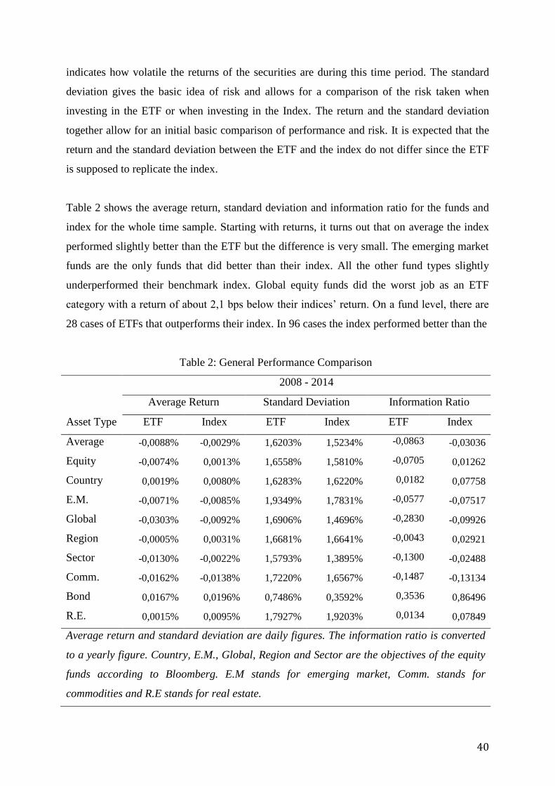
40

indicates how volatile the returns of the securities are during this time period. The standard

deviation gives the basic idea of risk and allows for a comparison of the risk taken when

investing in the ETF or when investing in the Index. The return and the standard deviation

together allow for an initial basic comparison of performance and risk. It is expected that the

return and the standard deviation between the ETF and the index do not differ since the ETF

is supposed to replicate the index.

Table 2 shows the average return, standard deviation and information ratio for the funds and

index for the whole time sample. Starting with returns, it turns out that on average the index

performed slightly better than the ETF but the difference is very small. The emerging market

funds are the only funds that did better than their index. All the other fund types slightly

underperformed their benchmark index. Global equity funds did the worst job as an ETF

category with a return of about 2,1 bps below their indices’ return. On a fund level, there are

28 cases of ETFs that outperforms their index. In 96 cases the index performed better than the

Table 2: General Performance Comparison

Asset Type

2008 - 2014

Average Return Standard Deviation Information Ratio

ETF Index ETF Index ETF Index

Average -0,0088% -0,0029% 1,6203% 1,5234% -0,0863 -0,03036

Equity -0,0074% 0,0013% 1,6558% 1,5810% -0,0705 0,01262

Country 0,0019% 0,0080% 1,6283% 1,6220% 0,0182 0,07758

E.M. -0,0071% -0,0085% 1,9349% 1,7831% -0,0577 -0,07517

Global -0,0303% -0,0092% 1,6906% 1,4696% -0,2830 -0,09926

Region -0,0005% 0,0031% 1,6681% 1,6641% -0,0043 0,02921

Sector -0,0130% -0,0022% 1,5793% 1,3895% -0,1300 -0,02488

Comm. -0,0162% -0,0138% 1,7220% 1,6567% -0,1487 -0,13134

Bond 0,0167% 0,0196% 0,7486% 0,3592% 0,3536 0,86496

R.E. 0,0015% 0,0095% 1,7927% 1,9203% 0,0134 0,07849

Average return and standard deviation are daily figures. The information ratio is converted

to a yearly figure. Country, E.M., Global, Region and Sector are the objectives of the equity

funds according to Bloomberg. E.M stands for emerging market, Comm. stands for

commodities and R.E stands for real estate.

41

ETF in terms of average daily return. More important however, is the fact that the returns of

the ETFs and their indices are generally extremely close. If there are any differences they are

very small and on a fund level they are generally less than 1 basis point except for the three

delisted SPA Marketgrader funds which show underperformance of 7 to 9 basis points (bps).

On average the return difference is less than 1 basis point at 0,59 bps.

When comparing the standard deviations much bigger differences present themselves. 82

ETFs display a higher volatility than their Index implying that 42 indices are more volatile

than their respective ETF. As shown in table 2 the difference in daily standard deviation can

reach up to roughly 39 basis points (bond funds). Equity funds and commodity funds

generally did quite well with an excess volatility of about 7 bps over their benchmark. Region

equity funds show the smallest difference in standard deviation at less than 1 basis point. This

difference in standard deviation is an indication that exchange-traded funds are more risky

than their underlying index.

The last two columns of table 2 show the average information ratio of the ETFs and the

indices. Due to the fact that standard deviations differed quite a lot but return differences were

small, the information ratio also shows a similar pattern as the standard deviation comparison.

When looking at the information ratios at a fund level, it turns out that 28 ETFs in the sample

offer a better risk-adjusted return than the actual index underlying that fund. This also implies

however that most (96) of the ETFs underperform their index when comparing them by

information ratio. This stands in contrast to the findings of Adjei (2009) in which ETFs

generally offered a higher reward for risk than the market. Another interesting feature is the

fact that 57 ETFs manage to offer a positive information rate whereas the other 67 managed to

deliver a negative information ratio. A negative information ratio basically means that there

was no compensation for the risk taken. According to table 2, country equity funds, bond

funds and real estate funds are the only asset classes that deliver a positive information ratio.

Global equity exchange-traded funds did the worst with an information ratio at -0,2830. This

figure is however very likely to be highly negatively influenced by the relatively short time

period which includes a major financial crisis that significantly depresses the performance.

The best performing ETF was the IShares Euro Government Bond 7-10, which delivered an

information ratio of 0,478 during this period. Among the top performers are mainly bond

ETFs: in the top 10% performers 6 are bond linked funds. During expansionary economic

however, the equity funds will probably perform better and outperform the bond ETFs. The

42

worst performing fund was the ETFS natural gas with an information ratio of -1,02. It is

striking to see that amongst the worst 10% performers, 7 ETFs were commodity funds. Next

to that, all of the 3 delisted SPA Marketgraders’ ETFs are amongst the worst 10 performers

with information ratios around -0,8.

The correlations between the return of the ETFs and their benchmarks have been calculated

and are shown in table 3. The correlations give an extra dimension to the previous return

comparison and are particularly important because of the great use of correlations in portfolio

management. By calculating the correlation between the ETFs and the benchmarks the extent

to which variation of the returns is replicated by the ETF can be determined. Table 4 shows

that on average the funds exhibit a very high correlation (89,40%) with their benchmark and

that all the correlation coefficient are significant and positive. Equity funds did the best as an

asset class and bond funds the worst. Within equity funds, the country funds did the best with

a correlation of 90,40%. It is worth noting that all equity funds seem to exhibit a relatively

high correlation to their benchmark. Even the emerging market funds, which may be expected

to have more troubles tracking their index, performed well. The lowest correlations among

equity funds are found in the global equity and sector funds, which have a correlation

coefficient of 76,80% and 77,70% respectively. The large group of commodity funds did well

and display a correlation of 85,60%. Bonds did not do great as shown by the correlation

coefficient of 57%, the lowest in the sample. The fact that the bond funds show the lowest

correlation may be surprising as most of them track sovereign fixed income securities form

major countries which may seem easy to track. On the other hand however, the general low

volatility of bond funds may be the reason that the correlations are so low as there is little

volatility to explain for. In general, the difference from a correlation of 1 implies that

investors should be careful with their expectations when including ETFs in their portfolio.

The ETFs do not offer the exact same risk and return characteristics as their benchmark and

thus may have slightly different implications for their portfolio and diversification motives.

Given that an ETF is expected to have the same return as its underlying index and solely

driven by the constituents’ return, it is expected that the beta of the regression (10) is equal to

one. Table 4 shows that this is not always the case. The full sample shows an average beta of

0,735. The beta closest to one is found in the bond funds. This stands in contrast to the much

poorer performance of bond funds in the correlation comparison. The lowest beta is found in

global equity funds. Interestingly, over the past six years the beta got closer to one for each

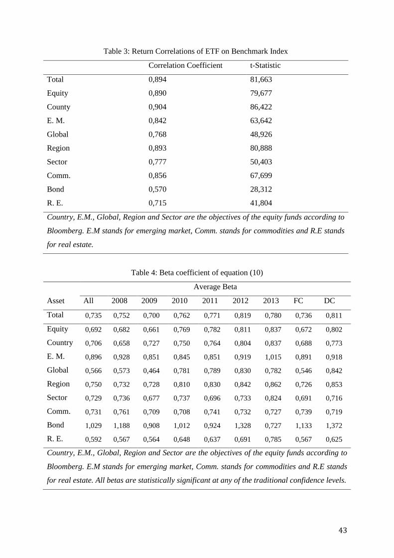
43

Table 3: Return Correlations of ETF on Benchmark Index

Correlation Coefficient t-Statistic

Total 0,894 81,663

Equity 0,890 79,677

County 0,904 86,422

E. M. 0,842 63,642

Global 0,768 48,926

Region 0,893 80,888

Sector 0,777 50,403

Comm. 0,856 67,699

Bond 0,570 28,312

R. E. 0,715 41,804

Country, E.M., Global, Region and Sector are the objectives of the equity funds according to

Bloomberg. E.M stands for emerging market, Comm. stands for commodities and R.E stands

for real estate.

Table 4: Beta coefficient of equation (10)

Average Beta

Asset All 2008 2009 2010 2011 2012 2013 FC DC

Total 0,735 0,752 0,700 0,762 0,771 0,819 0,780 0,736 0,811

Equity 0,692 0,682 0,661 0,769 0,782 0,811 0,837 0,672 0,802

Country 0,706 0,658 0,727 0,750 0,764 0,804 0,837 0,688 0,773

E. M. 0,896 0,928 0,851 0,845 0,851 0,919 1,015 0,891 0,918

Global 0,566 0,573 0,464 0,781 0,789 0,830 0,782 0,546 0,842

Region 0,750 0,732 0,728 0,810 0,830 0,842 0,862 0,726 0,853

Sector 0,729 0,736 0,677 0,737 0,696 0,733 0,824 0,691 0,716

Comm. 0,731 0,761 0,709 0,708 0,741 0,732 0,727 0,739 0,719

Bond 1,029 1,188 0,908 1,012 0,924 1,328 0,727 1,133 1,372

R. E. 0,592 0,567 0,564 0,648 0,637 0,691 0,785 0,567 0,625

Country, E.M., Global, Region and Sector are the objectives of the equity funds according to

Bloomberg. E.M stands for emerging market, Comm. stands for commodities and R.E stands

for real estate. All betas are statistically significant at any of the traditional confidence levels.

44

asset class and the total sample’s beta was closest to one in 2012. The total sample only shows

a small improvement but individual asset classes such as real estate and equity funds show

major improvements. During the financial crisis the lowest betas are found. During the debt

crisis on the other hand, the beta is high and does not seem to be affected by the crisis. Except

for the bond funds, the implications taken from correlations between the returns are consistent

with the betas in table 3. On average, both the betas and the correlations only differ slightly

from one.

NAV discrepancies

The NAV discrepancy will be given as the log difference or in basis points and will be

displayed in graphs rather than tables. The use of graphs is preferred over tables in order to

spot trends over time and to see intra-year volatility. All funds together have an average log

premium of 0,624. Most funds show very low average discounts or premiums but some funds

show high discrepancies between the intrinsic value and the market price with a log price

difference of more than 4,6. Within the sample the commodity funds and the fixed income

funds have been doing much better than equity ETFs. All commodity funds show a very low

discrepancy with an average premium of just 0,0025. Fixed income funds show an average

discount of a tiny 0,0008. IBTM LN is the fund with the lowest average difference between

NAV and market price. Other funds that see only a very small difference on average are IBTS

LN, IDJG LN, DJMC LN and AIGX LN. Equity, bond and commodity funds are all featured

in the bottom group of discount/premium to NAV. The 5 funds that experience the largest

discrepancies are LFAS LN, LBRZ LN, LCNE LN, L250 LN and LNFT LN, with the fund

with the highest difference first. Interestingly all these 5 funds are equity funds and managed

by Powershares and show an average premium around 4,6. Next to that 3 of the bottom 5

funds have been delisted over time.

The development over time of the discount and premium should be considered as it will show

whether there is any improvement over time and whether it is fair to expect the price

discrepancy to grow or to shrink in the future. As ETFs matured and grew in use and

acceptance by investors, the creation and redemption activity may have increased, preventing

the existence of (substantial) price premiums or discounts. The development of the average

discount or premium for the major asset classes except real estate is presented next. Real

estate will not be displayed because of the low amount of funds (4) focusing on real estate.

Figure 1: Equity ETFs’ Average Price Premium or Discount

0

0.2

0.4

0.6

0.8

1

1.2

1.4

1/2/08

1/2/09

1/2/10

1/2/11

1/2/12

1/2/13

1/2/14

EquityAveragePremium/Discount

46

Figure 2: Commodity ETFs’ Average Price Premium or Discount

-0.05

-0.04

-0.03

-0.02

-0.01

0

0.01

0.02

0.03

0.04

0.05

0.06

1/2/08

1/2/09

1/2/10

1/2/11

1/2/12

1/2/13

1/2/14CommodityAveragePremium/Discount

47

Figure 3: Bond ETFs’ Average Price Premium or Discount

-0.035

-0.03

-0.025

-0.02

-0.015

-0.01

-0.005

0

0.005

0.01

0.015

1/2/08

1/2/09

1/2/10

1/2/11

1/2/12

1/2/13

1/2/14BondAveragePremium/Discount

48

Figure 4: Full Sample Average Price Premium or Discount

0

0.1

0.2

0.3

0.4

0.5

0.6

0.7

0.8

1/2/08

1/2/09

1/2/10

1/2/11

1/2/12

1/2/13

1/2/14AveragePremium/Discount

Figure 1 shows the NAV discrepancy over time for the 51 equity funds in the sample. It is

clear that the equity funds perform quite poorly and they are the reason that the total sample

displays such high discounts and premiums. According to the figure, there has always been a

premium for equity funds indicating that the price of the equity ETFs is generally higher than

the NAV of the funds. The premium seems to be relatively stable and in particular since 2013

seems to be very close to 100 bps. No trend can be spotted and a decline of this premium is

not expected in the near future from this figure.

Figure 2 shows the development for the 45 commodity ETFs in the sample. It seems that the

average discrepancy between the ETC prices and their NAVs has decreased over time. Over

the first year, the difference was volatile with a peak premium around 5 bps and a low at a

discount of about 4 bps. Since 2009, the difference seems to have settled down and fluctuated

just slightly around 0 with no major peaks or outliers anymore. This would indicate that the

commodity funds are operating efficiently and that the creation and redemption process works

well for these funds.

Figure 3 shows the average discount or premium of the 10 fixed income/bond funds in the

sample. 10 is a low number to take general conclusions from but for the bond funds included

in the sample it seems that their premium or discount is generally close to non-existent. It is

very interesting to see that during the financial crisis it seems that the price dropped more than

the NAV of the bond funds, indicating that bond ETF prices dropped relative to their NAV

during this period. The biggest discount achieved during the financial crisis was around 3 bps.

A similar negative spike can be seen among the commodity funds. The fact that the bonds

funds show the biggest discount during the financial crisis is surprising at first as it is

expected that investors move to more safe assets such as investment grade fixed income

securities. Especially given the fact that the bond funds in the sample are centered on some of

the most developed markets in the world, such a discount is not expected. Perhaps as a

extreme flight to safety investors sold off all financial instruments (including bond ETFs) to

get cash as ETFs may have not been considered safe enough despite the fact that they are

tracking bond indices. Nevertheless, after the crisis the premium/discount returned back to

around 0 and remained like this for the rest of the time period. Contrary to the financial crisis,

during the European sovereign debt crisis there was no sign of an increased premium or

discount for the 10 bond ETFs.

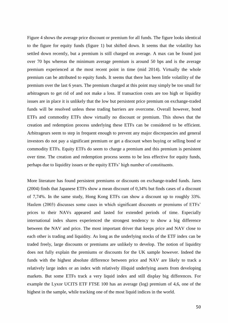
50

Figure 4 shows the average price discount or premium for all funds. The figure looks identical

to the figure for equity funds (figure 1) but shifted down. It seems that the volatility has

settled down recently, but a premium is still charged on average. A max can be found just

over 70 bps whereas the minimum average premium is around 50 bps and is the average

premium experienced at the most recent point in time (mid 2014). Virtually the whole

premium can be attributed to equity funds. It seems that there has been little volatility of the

premium over the last 6 years. The premium charged at this point may simply be too small for

arbitrageurs to get rid of and not make a loss. If transaction costs are too high or liquidity

issues are in place it is unlikely that the low but persistent price premium on exchange-traded

funds will be resolved unless these trading barriers are overcome. Overall however, bond

ETFs and commodity ETFs show virtually no discount or premium. This shows that the

creation and redemption process underlying these ETFs can be considered to be efficient.

Arbitrageurs seem to step in frequent enough to prevent any major discrepancies and general

investors do not pay a significant premium or get a discount when buying or selling bond or

commodity ETFs. Equity ETFs do seem to charge a premium and this premium is persistent

over time. The creation and redemption process seems to be less effective for equity funds,

perhaps due to liquidity issues or the equity ETFs’ high number of constituents.

More literature has found persistent premiums or discounts on exchange-traded funds. Jares

(2004) finds that Japanese ETFs show a mean discount of 0,34% but finds cases of a discount

of 7,74%. In the same study, Hong Kong ETFs can show a discount up to roughly 33%.

Haslem (2003) discusses some cases in which significant discounts or premiums of ETFs’

prices to their NAVs appeared and lasted for extended periods of time. Especially

international index shares experienced the strongest tendency to show a big difference

between the NAV and price. The most important driver that keeps price and NAV close to

each other is trading and liquidity. As long as the underlying stocks of the ETF index can be

traded freely, large discounts or premiums are unlikely to develop. The notion of liquidity

does not fully explain the premiums or discounts for the UK sample however. Indeed the

funds with the highest absolute difference between price and NAV are likely to track a

relatively large index or an index with relatively illiquid underlying assets from developing

markets. But some ETFs track a very liquid index and still display big differences. For

example the Lyxor UCITS ETF FTSE 100 has an average (log) premium of 4,6, one of the

highest in the sample, while tracking one of the most liquid indices in the world.

51

Tracking Error

The tracking error shows how accurately an exchange-traded fund tracks its benchmark.

Perfect funds that mimic their benchmark exactly offer the same return as their benchmark

index and do not exhibit any tracking error at all. In general when the absolute tracking error

(TE 2) is close to zero, the fund does a good job in tracking the index. The tracking error is

also a term widely used to represent the volatility of returns of the ETF relative to the

benchmark and thus often expressed as a standard deviation of the return differences (TE 3)

(Mussavian and Hirsch, 2002). All five methods for approximating the tracking error will be

discussed next.

Method 1 - Simple Tracking error

Figure 5 shows the development of the average simple tracking error over time. Upon first

sight it seems that the funds track their benchmark very well. The mean average tracking error

is tiny at 0,34 basis points. One can see that it appears to be the case that ETFs have gotten

slightly better in tracking their index as time went by and the average tracking error seems to

fluctuate around 0. The average tracking error seems to be within a band of +100 basis points

to -100 basis points with some spikes during the crisis in 2008 and 2009 but narrows down to

a band of roughly +50 basis points and -50 basis points from 2010 onwards. During the

financial crisis volatility increases and the biggest spikes appear. A maximum is found around

0,03 (316 basis points) and the minimum is at -0,02 (-236 basis points). This gives a first

indication that during crisis periods tracking ability gets disturbed and more difficult

compared to calmer economic periods.

Figure 6 shows the distribution of the return difference or the average tracking error over the

full range of funds. Given that the simple tracking error can be both positive and negative, a

histogram is a useful figure to include and analyse. The curved line represents the normal

distribution and the blue bars the actual sample distribution. The average tracking error tends

to be slightly negative, indicating that the funds generally have a lower return than the return

achieved by the index. There are no big spikes or outliers at the more extreme ends of the

spectrum. The fact that the average tracking error tends to be slightly below zero is coherent

with the results found in the return comparison previously (Table 2), where the majority of the

ETFs slightly underperformed their benchmark index.

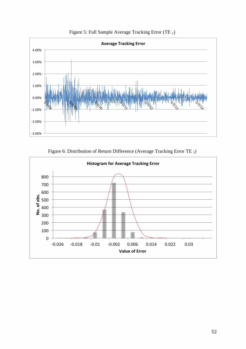
52

Figure 5: Full Sample Average Tracking Error (TE 1)

Figure 6: Distribution of Return Difference (Average Tracking Error TE 1)

-3.00%

-2.00%

-1.00%

0.00%

1.00%

2.00%

3.00%

4.00%

1/2/08

1/2/09

1/2/10

1/2/11

1/2/12

1/2/13

1/2/14AverageTrackingError

0

100

200

300

400

500

600

700

800

-0.026 -0.018 -0.01 -0.002 0.006 0.014 0.022 0.03

No.o

fobs.

ValueofError

HistogramforAverageTrackingError

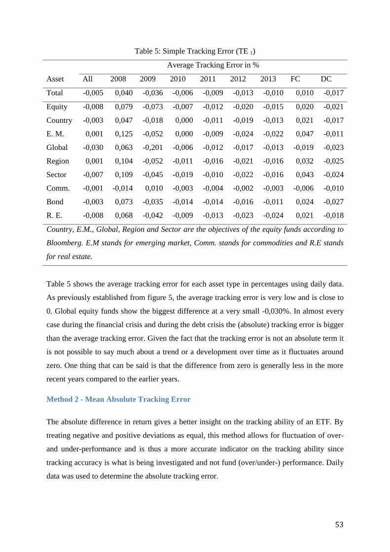
53

Table 5: Simple Tracking Error (TE 1)

Average Tracking Error in %

Asset All 2008 2009 2010 2011 2012 2013 FC DC

Total -0,005 0,040 -0,036 -0,006 -0,009 -0,013 -0,010 0,010 -0,017

Equity -0,008 0,079 -0,073 -0,007 -0,012 -0,020 -0,015 0,020 -0,021

Country -0,003 0,047 -0,018 0,000 -0,011 -0,019 -0,013 0,021 -0,017

E. M. 0,001 0,125 -0,052 0,000 -0,009 -0,024 -0,022 0,047 -0,011

Global -0,030 0,063 -0,201 -0,006 -0,012 -0,017 -0,013 -0,019 -0,023

Region 0,001 0,104 -0,052 -0,011 -0,016 -0,021 -0,016 0,032 -0,025

Sector -0,007 0,109 -0,045 -0,019 -0,010 -0,022 -0,016 0,043 -0,024

Comm. -0,001 -0,014 0,010 -0,003 -0,004 -0,002 -0,003 -0,006 -0,010

Bond -0,003 0,073 -0,035 -0,014 -0,014 -0,016 -0,011 0,024 -0,027

R. E. -0,008 0,068 -0,042 -0,009 -0,013 -0,023 -0,024 0,021 -0,018

Country, E.M., Global, Region and Sector are the objectives of the equity funds according to

Bloomberg. E.M stands for emerging market, Comm. stands for commodities and R.E stands

for real estate.

Table 5 shows the average tracking error for each asset type in percentages using daily data.

As previously established from figure 5, the average tracking error is very low and is close to

0. Global equity funds show the biggest difference at a very small -0,030%. In almost every

case during the financial crisis and during the debt crisis the (absolute) tracking error is bigger

than the average tracking error. Given the fact that the tracking error is not an absolute term it

is not possible to say much about a trend or a development over time as it fluctuates around

zero. One thing that can be said is that the difference from zero is generally less in the more

recent years compared to the earlier years.

Method 2 - Mean Absolute Tracking Error

The absolute difference in return gives a better insight on the tracking ability of an ETF. By

treating negative and positive deviations as equal, this method allows for fluctuation of over-

and under-performance and is thus a more accurate indicator on the tracking ability since

tracking accuracy is what is being investigated and not fund (over/under-) performance. Daily

data was used to determine the absolute tracking error.

54

Table 6: Absolute Tracking Error (TE 2)

Absolute Average Tracking Error in %

Asset All 2008 2009 2010 2011 2012 2013 FC DC

Total 0,802 1,237 1,056 0,686 0,711 0,535 0,481 1,201 0,638

Equity 0,833 1,303 1,109 0,637 0,682 0,474 0,457 1,255 0,608

Country 0,752 1,324 0,928 0,617 0,659 0,483 0,418 1,171 0,621

E. M. 0,783 1,341 1,054 0,656 0,707 0,498 0,536 1,256 0,666

Global 1,098 1,351 1,555 0,599 0,627 0,408 0,437 1,451 0,516

Region 0,787 1,209 1,003 0,655 0,682 0,480 0,470 1,171 0,608

Sector 0,683 1,306 0,963 0,642 0,771 0,488 0,502 1,245 0,634

Comm. 0,830 1,238 1,049 0,789 0,804 0,663 0,547 1,194 0,730

Bond 0,416 0,580 0,577 0,431 0,396 0,280 0,282 0,623 0,338

R. E. 0,959 1,914 1,569 0,737 0,765 0,463 0,494 1,943 0,688

Country, E.M., Global, Region and Sector are the objectives of the equity funds according to

Bloomberg. E.M stands for emerging market, Comm. stands for commodities and R.E stands

for real estate.

Table 6 shows that the absolute tracking error is generally quite low with an average at about

0,80%. This is still quite a low tracking error but significantly higher than the tracking error

established using the previous simple difference approximation method. Over time the

tracking error decreased and the financial crisis shows the second largest absolute tracking

error. The high tracking error during the financial crisis is not only appearing in the total

sample but also seen in the separate asset classes. The European sovereign debt crisis period

shows a tracking error which is a lot lower than the tracking error during the financial crisis

and not much different from the performance of the funds during the most recent years. Hence

it seems that only the first crisis has an effect on the tracking error according to the measure.

According to the absolute tracking error method, the best tracking fund was the IShares FTSE

100-inc, an exchange-traded funds that tries to replicate the FTSE 100 index. The fund

performed extremely well in tracking the major index of the United Kingdom and as seen

before it is also the most traded ETF on the London Stock exchange. Whether this high

trading volume and liquidity has a significant impact on the tracking error will be investigated

later. Amongst the best 10% performing funds on the basis of tracking error (TE 2) it is

55

interesting to see that many of the funds have a focus on the UK market. Amongst these best

firms there are UK equity, UK fixed income and even UK real estate ETFs. So irrespective of

the underlying asset type, tracking performance has been good for these UK-focused funds.

Other good performing funds were government bond ETFs with the UK and euro government

bonds performing the best. Amongst the worst performing 10%, six funds have been delisted

now. Again all three funds offered by SPA Marketgrader performed poorly similar to some

commodity ETFs. Next to that, three delisted ETFs formerly offered by Lyxor that covered

developing markets display a relatively high tracking error with for example the Lyxor ETF

MSCI AC Asia Pacific excluding Japan having an average tracking error during this sample

period of 1,75%. The list of worst performers is completed by commodity funds and one US

real estate fund.

Figure 7 shows the development of the average absolute tracking error for the full sample

over time. There are spikes and high volatility around the financial crisis period similar to

figure 5. Looking at figure 7 there seems to be little effect from the European sovereign debt

crisis on the tracking performance of the sample, also similar to the results found using the

simple tracking error estimate and displayed in figure 5. More generally, it is fair to conclude

that tracking performance is quite stable and relatively accurate for the sample of ETFs.

Figure 7: Full Sample Average Absolute Tracking Error (TE 2)

0.00

0.01

0.02

0.03

0.04

1/2/08

1/2/09

1/2/10

1/2/11

1/2/12

1/2/13

1/2/14

AverageAbsoluteTrackingError

56

From figure 7 and table 6 it seems that tracking performance improves over time. The

tracking error in 2013 is a lot lower than the tracking error in 2008. This applies to the full

sample but also for every single asset class. The difference between 2008 and 2013 can be

very large, in some cases the 2008 tracking error is almost 3 times as big as the 2013 tracking

error. When looking at a funds level there is a general trend to perform better over time but

there also seems to be some persistence in tracking performance. 6 of the best 10%

performers are among the best 10% every single year and during the crisis periods. For the

worst performers there is less consistency compared to top performers. The ETFS physical

silver and natural gas do perform very poorly however and are among the worst in most years.

Other funds that consistently performed poorly are mainly delisted funds. For example some

of the Lyxor funds such as the Lyxor ETF Brasil and the three SPA Marketgrader funds did

poorly every single year.

Method 3 - Standard Deviation of Return Differences

In general the lower the standard deviation of return differences, the better the tracking

accuracy. Table 7 shows the development of the standard deviation in return differences over

time for the sample of ETFs (using daily data). Similar to the conclusions drawn from the

previous methods, tracking performance improved over time. The more recent figures of the

tracking error are significantly better than the ones in 2008. During the financial crisis period

the standard deviation is much high than the average tracking error for all asset types. This

indicated that during the financial crisis, fund managers found it increasingly difficult to track

their index and limit volatility around the index return. During the debt crisis there is no sign

of significantly increased volatility.

The best and worst 10% performers are similar to the ones found using the second method of

tracking error. The very best performer was the iShares FTSE 100 ETF with a standard

deviation of 0,0020. Other great performers were the iShares UK GILTS (0,0026), iShares

GBP Index-Linked GIL (0,0035) and the iShares FTSE 250 ETF. The well performing ETFs

are mainly fixed income funds or funds focusing on extremely liquid and large indices.

Similar to method 2 the worst performers are the delisted SPA Marketgrader funds, three of

the delisted emerging market ETFs offered by Lyxor and some commodities such as ETFS

natural gas (0,0214) and ETFS silver (0,0224) which were also among the bottom 10%

performers using the previous measure. It is interesting to see that among the best performers

57

Table 7: Standard Deviation of Return Differences (TE 3)

Standard Deviation in %

Asset All 2008 2009 2010 2011 2012 2013 FC DC

Total 1,272 1,889 1,526 0,882 0,941 0,695 0,598 1,807 0,837

Equity 1,341 1,923 1,590 0,777 0,890 0,605 0,520 1,853 0,782

Country 1,235 2,001 1,363 0,882 0,977 0,644 0,476 1,844 0,849

E. M. 1,142 1,943 1,373 0,863 0,944 0,635 0,672 1,758 0,871

Global 1,887 2,211 2,753 0,537 0,605 0,377 0,410 2,479 0,484

Region 1,184 1,859 1,333 0,818 0,886 0,622 0,556 1,669 0,779

Sector 1,062 1,285 0,826 0,734 1,094 0,814 0,679 1,190 1,036

Comm. 1,282 1,930 1,538 1,071 1,081 0,879 0,732 1,821 0,971

Bond 0,629 0,943 0,824 0,559 0,520 0,378 0,385 0,953 0,466

R. E. 1,721 3,230 2,143 0,976 1,069 0,613 0,669 3,073 0,967

Country, E.M., Global, Region and Sector are the objectives of the equity funds according to

Bloomberg. E.M stands for emerging market, Comm. stands for commodities and R.E stands

for real estate.

there seems to be a degree of performance persistency over time. Of the top performers 4

funds manage to be in the top 10% during every single year and during the 2 crisis periods,

examples of such funds are the iShares FTSE 100 and the iShares FTSE 250 ETFs. There is

less persistency among the worst performers. None of the worst performing funds are among

the bottom 10% every single period. ETFS physical silver however, is among the worst 10%

in every year except for 2009. Also when looking at yearly performance the best and worst

funds are very similar to the ones using the absolute differences method (TE 2).

Method 4 - R-Squared

The R-squared (R2), also called the coefficient of determination, shows how much of the

data’s variation is explained for by the model. The closer to 100%, the better the model

captures the variation. The return of exchange-traded funds should just depend on the return

of the underlying index if the fund does a good job in tracking the index. Consequently, it is

expected that the R-squared is very close to 1. High deviations from 1 may be an indication

that the ETF is performing poorly in replicating its benchmark portfolio.

58

Table 8: Coefficient of Determination (R2) (TE 4)

R-Squared in % of (11)

Asset All 2008 2009 2010 2011 2012 2013 FC DC

Total 47,9 47,1 48,8 53,3 58,4 59,1 53,8 46,9 58,9

Equity 50,9 50,5 51,0 57,7 63,1 63,8 57,7 50,5 64,7

Country 52,2 49,7 51,3 57,0 62,5 64,5 64,9 47,7 62,1

E. M. 66,5 71,1 59,7 59,5 65,1 67,9 63,3 69,7 66,5

Global 39,8 40,1 42,6 59,2 64,3 65,5 49,8 39,3 69,5

Region 57,7 57,9 55,9 62,0 67,2 65,6 60,2 58,4 68,6

Sector 35,7 49,3 51,2 47,7 53,9 55,2 47,9 48,5 56,7

Comm. 51,2 48,9 51,9 54,1 58,7 57,8 55,2 49,1 56,3

Bond 27,8 26,3 23,2 27,0 33,6 43,9 30,3 25,6 43,8

R. E. 37,5 29,0 43,9 47,4 51,0 47,7 48,1 34,2 47,8

Country, E.M., Global, Region and Sector are the objectives of the equity funds according to

Bloomberg. E.M stands for emerging market, Comm. stands for commodities and R.E stands

for real estate. Individual years have at least 250 observations, the total sample 1670

observations and FC and DC have at least 375 and 175 observations respectively.

Table 8 shows that the R-squared statistic is never close to 1 and an average R-squared of

0,479 indicates that the ETFs did quite poorly in tracking their index according to this

method. Consistent with previous tracking error estimates, the best performing fund is the

IShares FTSE-100 ETF with an R-squared of 0,978. The worst performing fund is the SMA

Marketgrader 200 with an R-squared of 0,005. The average R-squared changes quite a lot

over time and ranges from a low of 0,469 during the financial crisis to 0,591 in 2012. Some

funds did not manage to improve tracking performance over time using the R-squared

measure. During the two crisis periods tracking performance differed quite a lot. The 2008

financial crisis was actually the worst period of all on a tracking error basis according to the

R-squared with an average R-squared of 46,9%. The lower R-squared values during the

financial crisis are coherent with the findings of Wong and Shum (2010) who found that the

R-squared generally drops during bearish periods. The European sovereign debt crisis

however, did not seem to have a negative impact on the tracking ability since the R-squared

during this period is the second to best. All asset types performed poorly but bond funds did

exceptionally bad according to this measure given by the R-squared of just 25,6%. This stands

59

in stark contrast against the tracking error found among the bond funds using other methods

in which bonds performed among the best. This shows that when estimating tracking

performance it is wise to use multiple tracking error approximation methods and not just one.

On a fund level, it is interesting to note that some funds do not seem to perform in a consistent

matter. For example the ETFS Lean Hogs (HOGS LN) performs poorly in the first two years

with an R-squared of 0,179 and 0,050 but manages to reach 0,528 in the 2013. Another

example of a fund that improved its performance a lot over time is ETFS Gold (BULL LN),

which moved from 0,566 in 2008 to 0,852 in 2013. Other funds do not show an upward trend

and actually perform worse and worse over time. For example, iShares Global Infrastructure

ETF (INFR LN) shows an R-squared of 0,611 in 2008, far above the sample average. In 2012

the R-squared dropped all the way to 0,010 and 0,317 in 2013. On average however, most

funds’ performance seems to be slightly improving or stable over time according to the R-

squared measure.

Method 5 - Standard Error

Table 9: Standard Error of Regression (TE 5)

Standard Error of (11)

Asset All 2008 2009 2010 2011 2012 2013 FC DC

Total 0,011 0,018 0,013 0,009 0,009 0,007 0,006 0,017 0,008

Equity 0,011 0,018 0,014 0,008 0,009 0,006 0,006 0,018 0,008

Country 0,011 0,018 0,013 0,008 0,009 0,006 0,005 0,017 0,008

E. M. 0,011 0,019 0,013 0,008 0,009 0,006 0,007 0,017 0,009

Global 0,013 0,019 0,020 0,008 0,008 0,005 0,006 0,023 0,007

Region 0,010 0,017 0,012 0,008 0,009 0,006 0,006 0,015 0,007

Sector 0,012 0,019 0,012 0,008 0,010 0,008 0,007 0,017 0,010

Comm. 0,012 0,018 0,014 0,010 0,010 0,008 0,007 0,017 0,009

Bond 0,006 0,009 0,008 0,006 0,005 0,004 0,004 0,009 0,005

R. E. 0,014 0,026 0,016 0,008 0,009 0,006 0,006 0,024 0,008

Country, E.M., Global, Region and Sector are the objectives of the equity funds according to

Bloomberg. E.M stands for emerging market, Comm. stands for commodities and R.E stands

for real estate. Individual years have at least 250 observations, the total sample 1670

observations and FC and DC have at least 375 and 175 observations respectively.

60

The standard error of the regression model (10) will be considered next. It gives the standard

deviation of the sampling distribution’s mean. The lower the standard error, the better the

ETF did in tracking the benchmark. According to table 9, the full sample shows an average

standard error of the regression of 0,011. In 2008 the SE is 0,0177 but overtime there is a

gradual improvement of performance as the SE goes down every year approaching zero. In

the last period, ranging from 2013 to mid- 2014, the average SE dropped to 0,0056. Each fund

category shows an improvement in tracking performance over time with very low standard

error estimates in the last two years, a fraction of the 2008 figures. During the financial crisis

the standard error is 0,0166, slightly lower than the 2008 figure but higher than the 2009

error. The Sovereign debt crisis shows a standard error of just 0,0075, which is the third to

lowest observation.

The very best performers are the ISF LN (0,0020), IGLT LN (0,0026) and the INXG LN

(0,0035) ETFs. Some of the worst performers are HOGS LN (0,0249), COTN LN (0,0204)

and the SPA Marketgrader funds, all five had standard errors slightly above 0,02. There is

some consistency when comparing the best and worst funds using the standard error measure

and other measures. For example six of the top 10% performers using the standard error

measure are also the best performers using the R-squared measure. Similarly, six funds are

among the worst 10% using both measures. Interestingly, the IBGS fund was among the worst

10% performers using the R-squared method but is in the top 10% of the standard error

method.

As indicated by Pope and Yadav (1994), the tracking error using this estimate may be

overstated if the beta of (10) is not equal to one. As shown in table 3 the beta is indeed not

equal to one indicating that the actual tracking error might be slightly lower than indicated by

table 8. By combining the results from the standard error of the regression with the other

methods however, a reliable conclusion on the final tracking error among the sample can still

be made by nuancing the implications retrieved from the standard error.

Market Volatility

In order to find out whether market volatility has an impact on the tracking error a correlation

matrix is created that compares the change in the implied volatility indices (the VIX and the

61

Table 10: Market Volatility Correlations

VIX V2X Credit Spread

Asset All FC DC All FC DC All FC DC

Total 0,059* 0,073 0,071 0,081** 0,118* 0,256** 0,052* 0,103* 0,019

Equity 0,069** 0,085 0,066 0,092** 0,12* 0,193** 0,063** 0,105* 0,063

Country 0,046 0,038 0,017 0,082** 0,108* 0,173* 0,071** 0,105* 0,045

E. M. 0,027 0,042 0,016 0,043 0,059 0,086 0,034 0,078 0,067

Global 0,069** 0,094 0,086 0,076** 0,095 0,173* 0,063** 0,11* 0,021

Region 0,073** 0,089 0,036 0,089** 0,101 0,143* 0,045 0,069 0,048

Sector 0,079** 0,106* 0,128 0,1** 0,156** 0,229* 0,042 0,075 0,08

Comm. 0,032 0,025 0,05 0,044 0,071 0,21* 0,021 0,06 -0,047

Bond 0,061* 0,121* 0,008 0,052* 0,043 0,167* 0,036 0,076 -0,049

R. E. 0,01 0,003 0,03 0,054* 0,093 0,185* 0,031 0,061 0,085

The correlations between the absolute tracking error and the change in the VIX, V2X and

credit spread are displayed in this table. Country, E.M., Global, Region and Sector are the

objectives of the equity funds according to Bloomberg. E.M stands for emerging market,

Comm. stands for commodities and R.E stands for real estate. * Denotes 5% statistical

significance and ** denotes 1% statistical significance.

V2X) and a credit spread against the tracking error. The tracking error in this case will be the

tracking error estimate using method 2, the absolute tracking error.

From table 10 one can see that there seems to be some evidence in favour of a positive impact

of market volatility on the tracking error. For the full time period, the total sample shows a

positive and significant (5%) correlation coefficient between the tracking error and the change

in the VIX. The V2X seems to exhibit higher correlations with the tracking error than the VIX

index does. The V2X shows a highly significant correlation to the tracking error as the

correlation coefficient is equal to 0,081 and significant at the 1% level. The credit spread has

a 5% significant coefficient of 0,052 and seems to be the least related to the tracking error of

the three market volatility proxies. Clearly the coefficients are very low and close to zero

indicating only a small effect of market volatility on the tracking error. Nevertheless, the

coefficients are always positive and some are highly significant giving proof of a positive

relation between the tracking error and the market volatility.

62

Interestingly, during the financial crisis the correlation is less significant and only remains in

place with the V2X and the credit spread. The lower significance may be due to a smaller

amount of observations compared to the full time period. Despite this it is interesting to see

that during the crises periods the coefficient generally goes up compared to the average

correlation. The change in the VIX does not seem to significantly correlate with the tracking

error during both the financial crisis and the debt crisis. Both correlation coefficients go up to

roughly 0,07 but are not significant. Contrary to the VIX correlations, the V2X figures show

highly significant positive correlations on the total fund sample during the two crisis periods.

During the debt crisis every asset class except emerging market funds shows a positive and

significant correlation between the tracking error and the change in the V2X, offering more

evidence on a positive relation between market volatility and the tracking error. During the

financial crisis only three asset classes show a significant correlation using the V2X. In total

there is a positive correlation of 0,118 between the change in the V2X and the tracking error,

the highest among the three during the financial crisis. Next to the financial crisis, during the

debt crisis there are is a highly significant (1%) and positive correlation of 0,256 between the

V2X and the tracking error. The credit spread only exhibits a significant and positive

correlation with the tracking error during the financial crisis (0,103 at 1%) and not during the

debt crisis.

On an asset class level, five out of nine fund-type tracking errors have a significant correlation

with the change in the VIX. Sector funds have the strongest correlation at 0,079 which is

significant at the 1% level. All funds except emerging market and commodity funds display a

positive and highly significant correlation with the V2X. Sector funds show the highest

correlation at 0,1 (1%). The credit spread variable is only significantly correlated with equity,

country and global funds, all three significant at the 1% level. The coefficients are generally

the closest to zero when using the credit spread. On a fund level, of the 124 funds, 47 funds

show a significant positive correlation at the 5% level between the change in the V2X and

their tracking error. 25 funds show a significant positive correlation at the 1% level. At the

0,1% confidence level, 11 funds are left that show a significant positive correlation. The

correlation coefficient is quite low however. On average the correlation coefficient is only

0,074 so the impact of the market volatility seems limited but is always positive. 19 funds

display a significant positive correlation coefficient at the 5% level between their tracking

error and the bond spread.

63

Determinants of the tracking error Table 11 shows the result of the tracking error regression (13). According to the R

2 the

explanatory power of the three regressions ranges from 0,430 to 0,660. This implies that 66%

(TE 5) of the variation in the tracking error can be explained by explanatory variables in this

model. Upon analysing the residuals and applying a White’s test however, it seems that there

is some degree of heteroskedasticity in the four explanatory variables. This calls for some

modifications to the model in order to make sure the statistical power is valid. Therefore, as a

first step, the model is estimated again using White’s standard errors, which are still biased

but much more reliable compared to the normal standard errors (White, 1980). White’s

standard errors adjust the t-statistic and make them more reliable. The standard and the

adjusted t-statistics are shown in Table 11, the heteroskedasticity adjusted ones are placed in

square brackets. In order to improve the model further, a log transformation is applied.

According to Gujarati (2012), a log transformation can reduce heteroskedasticity in the

residuals. The adjusted regression model looks as follows:

ln(TE) = β0 + β1* ln (EXPi) + β2* ln (RISKi) + β3* ln (SIZEi) + β4* ln (dVOLi) + εi (14)

Table 12 shows the result of the adjusted regression (14). The adjustments decreased the

heteroskedasticity significantly, and the outcome from the White test improved. For the TE2

and TE4 models there is still some degree of heteroskedasticity as the White test shows that

the probability of all betas not being equal to zero is 7,8% and 8,7% respectively. Therefore

the White heteroskedasticity-consistent standard errors are used again and the resulting t-

statistics are also shown in table 12. Given the fact that the differences between the normal

and the robust t-statistics are small and since the model has been adjusted using logarithmic

transformation the results should be valid now and the implications can be discussed.

As seen from table 11 and table 12, the constant is close to zero and three out of the four

independent variables seem to be highly significant on every tracking error measure. There do

not seem to be major differences when using the normal standard errors or the

heteroskedasticity-robust standard errors. The sign of each of the independent variables does

never flip in any of the models, showing consistency across the models and the variables. The

most significant factor is the standard deviation of the returns of the ETF, which proxies the

64

Table 11: Tracking Error Regression (13)

Dependent

Variables

Independent Variables

Constant EXP RISK SIZE DVOL R2

TE 2 -0,002

(-0,809)

[-0,771]

0,825***

(3,760)

[3,393]

0,382***

(4,121)

[3,987]

-0,000

(-0,275)

[-0,297]

-0,105

(-1,212)

[-1,010]

0,430

TE 3 -0,005

(-1,728)

[-1,543]

1,096**

(3,039)

[2,540]

0,856***

(5,606)

[5,423]

0,000

(0,377)

[0,415]

-0,358**

(-2,511)

[-2,075]

0,468

TE 5 -0,002

(-1,486)

[-1,662]

0,439**

(2,410)

[2,536]

0,743***

(9,633)

[8,247]

0,000

(0,663)

[0.784]

-0,202 ***

(-2,797)

[-2,682]

0,660

The tracking error is the dependent variable and is equal to the average of the tracking error of

each individual fund in the sample over the full time period. The independent variables are the

average risk of the ETF, the yearly expenses, average AUM and the average intraday

volatility of prices. The coefficients are displayed as the first number, the numbers in

parentheses are the t-statistics and the numbers in square brackets are the t-statistics using

White’s heteroskedasticity-consistent standard errors. * Denotes 10% statistical significance,

** denotes 5% statistical significance and *** denotes 1% statistical significance using

White’s standard errors.

risk of that ETF and is significantly positive at 1% statistical significance in each model. The

high importance of the risk of the ETF is consistent with finding by Milonas and Rompotis

(2006) and Rompotis (2012). The second explanatory variable, the total expense ratio, also

has a positive effect on the tracking error and is highly significant in all three models. Similar

to Frino and Gallagher (2001) but contrary to Rompotis (2009) there is a positive relation

between the expense ratio and the tracking error, implying that funds with lower expenses are

more likely to track their index better compared to more expensive funds. This result stands in

contrast to Shin and Soydemir (2010) who do not find a significant relation between the

expenses and the tracking error. Interestingly the fourth independent variable, the daily

volatility of the ETF price, seems to be highly significant and much more important than Shin

and Soydemir initially documented. Daily volatility of the price has a negative effect on the

tracking error significant at the 1% level in most models. This strong relationship is most

65

Table 12: Adjusted Tracking Error Regression (14)

Dependent

Variables

Independent Variables

Constant ln(EXP) ln(RISK) ln(SIZE) ln(DVOL) R2

ln(TE 2) 0,149

(0,239)

[0,235]

0,440***

(3,106)

[2,985]

0,824***

(5,208)

[5,611]

0,018

(0,264)

[0,429]

-0,121***

(-2,677)

[-3,138]

0,474

ln(TE 3) 0,348

(0,623)

[0,741]

0,273**

(2,145)

[2,349]

0,981***

(6,899)

[7,911]

0,017

(0,269)

[0,377]

-0,128***

(-3,142)

[-3,142]

0,523

ln(TE 5) -0,010

(-0,222)

[-0,225]

0,191**

(1,928)

[2,301]

0,947***

(8,563)

[10,976]

0,015

(0,318)

[0.574]

-0,087 ***

(-2,766)

[-3,817]

0,598

The tracking error is the dependent variable and is equal to the natural logarithm of the

average of the tracking error of each individual fund in the sample over the full time period.

The independent variables, all natural logarithms, are the average risk of the ETF, the yearly

expenses, average AUM and the average intraday volatility of prices. The coefficients are

displayed as the first number, the numbers in parentheses are the t-statistics and the numbers

in square brackets are the t-statistics using White’s heteroskedasticity-consistent standard

errors. * Denotes 10% statistical significance, ** denotes 5% statistical significance and ***

denotes 1% statistical significance using White’s standard errors.

likely because high daily price volatility indicates high trading activity and liquidity, which

should improve tracking performance according to Beutow and Henderson (2012). Unlike the

results found by Chu (2011) and Drenovak et al. (2012), fund size has absolutely no effect on

the tracking error in any of the models with a coefficient very close to 0.

Next to the four previously discussed sources for the tracking error, three other factors have

been tested for potential explanatory power on the tracking error. Contrary to the previously

discussed sources, the following three factors received none or very little attention in previous

academic literature. None of these three variables exhibit any significant effect on the tracking

error however, and therefore they are not displayed in any of the tables. The average daily

trading volume was included as it is a proxy for liquidity. According to Beutow and

Henderson (2012) improved liquidity should be beneficial for tracking performance. When

testing the effect of trading volume however, no significant results were found. This indicates

66

that in this sample the trading volume does not seem to be a key driver of tracking

performance. The average bid-ask spread was also included and is another proxy for liquidity.

A higher bid-ask spread generally indicates lower liquidity. Following the same logic as

before and depicted by Beutow and Henderson, a higher bid-ask spread should increase the

tracking error. The results from additional regressions did not show any relation between the

spread on the tracking error as the spread’s coefficient was insignificant and close to zero.

Finally the average price premium or discount to NAV discussed previously was included as a

potential source for tracking error. One might expect that the funds with the lowest price

discrepancies, and thus the most efficient funds, show a lower tracking error than other funds

as they may be more dedicated and more sophisticated. Rompotis (2012) indeed finds that the

absolute premium has a significant and positive effect on the tracking error. Similar to the

volume and bid-ask spread however, no significant result was found when including a price

premium or discount variable to the model.

Discussion and Implications

Investors can learn several things form the previously shown results. From the general

performance analysis it is fair to conclude that the exchange-traded funds manage to deliver

returns close to the return of their index. Very marginal return differences can be spotted over

the range of ETFs. This implies that investors are receiving the return they are expecting, and

paying for. This is the first indication that ETFs seem to replicate the benchmark returns well.

It does appear to be the case however, that ETFs display a much higher volatility than their

benchmark indices do. This underperformance in risk means that on a risk-return basis,

indices dominate ETFs. In sophisticated trading strategies however, volatility filters and good

funds selection can limit the higher risk of ETFs up to some extent. Nevertheless, for

investors this means that they should not assume identical risk between ETFs and indices.

This may have further implications for portfolio management and risk management issues.

From the analysis of betas and correlations it is confirmed that most funds exhibit a return

similar to their benchmark but there is no such thing as perfect replication here. ETF return

variation cannot be fully accounted for by index returns as shown by betas different from one

and correlations below one. In conclusion, investors should be careful with their expectations

from including exchange-traded funds in their portfolio. ETF return is close to the index

return but they will not exactly match the benchmark’s risk-and-return characteristics that are

so crucial in portfolio management.

67

Next to the fact that investors must be aware that ETFs do not exactly replicate the index one

to one on a risk-and-return basis, they should know that the funds may not be completely

efficient as shown by persistent price to NAV premiums and discounts. It must be said

however, that it is mainly the equity funds that generally trade at a premium. Commodity and

bond funds show a significantly lower discrepancy compared to equity funds. In the UK

sample equity funds charge about 100 bps over their net asset value, whereas other funds

show a price difference close to 0 bps. In theory the high difference between the price and the

NAV should not be possible due to the creation and redemption process which is deemed to

be efficient. The fact that authorised participants do not remove this arbitrage opportunity is

thus unexpected and puts the efficient nature of ETFs in a bad light. The fact that there does

not seem to be a downward trend in the price discrepancy makes it hard to believe the pricing

inefficiency will be removed in the very near future.

As shown in table 12, it seems that not all exchange-traded funds listed on the London Stock

Exchange are able to track their index accurately. Using multiple tracking error estimation

methods a relatively coherent picture can be drawn. In general the sample of ETFs performs

Table 13: Tracking Error Summary

Method TE 1 (%) TE 2 (%) TE 3 (%) TE 4 (%) TE 5

Total -0,005 0,802 1,272 47,9 0,011

Equity -0,008 0,833 1,341 50,9 0,011

Country -0,003 0,752 1,235 52,2 0,011

E. M. 0,001 0,783 1,142 66,5 0,011

Global -0,030 1,098 1,887 39,8 0,013

Region 0,001 0,787 1,184 57,7 0,010

Sector -0,007 0,683 1,062 35,7 0,012

Comm. -0,001 0,830 1,282 51,2 0,012

Bond -0,003 0,416 0,629 27,8 0,006

R. E. -0,008 0,959 1,721 37,5 0,014

Country, E.M., Global, Region and Sector are the objectives of the equity funds according to

Bloomberg. E.M stands for emerging market, Comm. stands for commodities and R.E stands

for real estate. Results for the full time period are displayed in this table.

68

quite well with an average absolute tracking error (TE 2) of 0,80% and a standard deviation of

return differences (TE 3) of 1,27%. It seems that region and country equity funds perform

quite well on each different tracking error method. Next to that, emerging market funds

performed surprisingly well and do not seem to be hindered by potential liquidity issues. The

broadest type of equity funds, global equity funds, generally had the biggest tacking error in

this sample. Bond funds did extremely well according to four out of five error estimates but

perform the worst according to the coefficient of determination (TE 4). This shows that big

differences can arise when analysing tracking performance while using different tracking

error estimates. Hence, it is suggested that other research keeps using multiple methods when

estimating tracking performance of funds in order to average out potential difference between

the methods. Regardless of the coefficient of determination, bond funds did exceptionally

well and offer investors easy and cheap access to bond exposure with very accurate tracking.

Commodities generally performed slightly better than equity funds and track their index

reasonably well. This implies that ETCs are a good way for investors to get exposure to

commodities while avoiding trading and handling difficulties attributed to traditional

commodities trading. A final positive note should be made about the tracking performance of

all ETFs. On average ETFs seems to get increasingly good in tracking their index as the total

average tracking error declined significantly over time. This improving tracking behaviour is

coherent with previous findings by Aroskar and Ogden (2012) who saw a similar

improvement over time. Despite the tracking improvement over time, investors should not

overlook the tracking error that can be seen over the whole range of ETFs. ETFs come with

attractive low explicit costs but the tracking error should be included as a hidden or implicit

cost.

Most of the tracking error that funds currently experience can be explained by three simple

factors. First of all the total expense ratio is a crucial driver for tracking performance. The

more an investor has to pay to the fund manager on a yearly basis, the worse the tracking

performance is, implying that cheaper funds perform better. This is most likely the case due to

the fact that the best performing funds are generally funds focusing on bond market or highly

liquid equity indices, which are the ones that charge the lowest fees. On the other hand, some

might be surprised that the cheapest funds perform best as they may expect the manager only

to charge more if the manager is highly skilled and likely to compensate for the higher costs

by offering better tracking accuracy. Next to fees, the risk or standard deviation of the returns

of the ETF has a very significant and positive effect on the tracking error: the higher the risk

69

of the ETF the worse tracking performance gets. Investors should therefore be cautious with

highly volatile and risky ETFs as their tracking error may be elevated. The final variable that

explains some of the tracking error is the daily ETF price volatility. If the intra-day price of an

ETF is volatile the tracking accuracy of that ETF gets better. This relation can most likely be

attributed to high trading activity and higher liquidity, which is generally good for tracking

performance according to Buetow and Henderson (2012).

The sample of funds has been picked in a way that they have been active for a sufficiently

long period in order to find out whether financial crises and highly volatile periods have an

impact on the tracking ability of exchange-traded funds. The results from the correlation

matrices indeed show that the tracking error is slightly positively correlated with market

volatility proxies such as implied volatility and the credit spread. This implies that investors

should be aware that during highly volatile times, the tracking performance of ETFs may be

sub-optimal and that they might want to avoid trading or holding exchange-traded funds

during these periods. Due to the lack of evidence from current literature on this matter, more

advanced time-series analysis between the market volatility and tracking ability of ETFs is

desired.

Conclusion

This study investigates the performance, pricing efficiency and tracking ability of exchange-

traded funds listed on the London Stock Exchange. In general, fund managers seem to have

performed quite well and made sure their ETFs under management tracked their benchmark

as seen by low tracking errors across the sample. The sample is not entirely free of some

degree of survivorship bias however, so conclusions about management performance should

not be made without caution. General performance and tracking accuracy on the other hand

are free to be discussed.

The performance comparison between ETFs and benchmark indices is done using risk and

return characteristics, betas and return correlations. As one would expect, according to the

sample results it seems that the ETFs offer virtually the same return as the indices but exhibit

higher volatility, resulting in a lower information ratio for ETFs compared to their

benchmarks. Most of the ETFs’ return can be attributed to index returns as shown by highly

positive correlations and betas close to one.

70

The unique creation and redemption mechanism underlying ETFs makes ETFs stand out from

the more traditional (index) mutual funds and should in theory prevent any pricing

discrepancies to arise. Despite the fact that this anti-arbitrage system is in place, it seems that

efficient pricing should not be taken for granted. In particular equity funds show consistent

and high pricing deviations with no apparent downward trend. Bond funds and ETCs

performed much better than equity funds and their pricing seems to be fully efficient.

The tracking error is one way to determine how well a fund does in tracking its benchmark

index. Five previously established tracking error approximations are used in this study and in

the end a relatively consistent result presents itself. Most funds did quite well in tracking their

index according to all but one tracking error (R-squared). More important is the fact that there

is a general improvement of tracking performance over time and significant advances have

been made. Nevertheless a small tracking error will still be present in the near future and

should be considered as a cost for investors. The main drivers for the tracking error are the

volatility of the ETF’s returns, daily price volatility and the total expense ratio. All factors

have a statistically significant impact on the tracking error. While the total expense ratio and

the risk have a positive impact, the daily price volatility has a negative impact on the tracking

error. Fund size, trading volume, average price premium or discount and the average bid-ask

spread did not have a significant impact on the tracking error.

By determining the tracking error during two economic crisis periods and by calculating the

correlation between the tracking error and market volatility proxies it is concluded that

exchange-traded funds struggle more in replicating their benchmarks’ return during volatile

periods. A positive and significant correlation between the implied market volatility and

tracking error can be found for most types of ETFs and some evidence comes from the

positive correlation between the credit spread and the tracking error. Similarly, during the

financial crisis period the tracking error peaked according to all five approximations of the

tracking error.

The results have several implications for investors. ETFs are a proven security for gaining

exposure to a desired market. Whether it is a country, a region or a sector, it is likely that an

ETF that tracks this market is available on the market. The funds offer this exposure and

diversification at very low costs while indeed performing close to the benchmark in terms of

71

return. Even for sophisticated or institutional investors, ETFs are a useful product since they

allows for active trading strategies, risk management, block trades and much more. On the

other hand, investors should be cautious about the pricing mechanism since consistent

premiums may be charged over the NAV. Next to that, there is a degree of tracking error but

this error is decreasing over time and getting very small. In crisis periods however, ETF

performance seems to worsen as displayed by increased tracking errors. Despite the price

premium and tracking error, it is fair to expect that the use of ETFs will remain popular due to

the wide range of advantages attributed to ETFs. The increase in use of ETFs may come at

continuing costs for traditional index funds until the clientele effect has fully developed and

separated the clientele of the two types of tracking funds.

There is room for more research on the subject of ETFs. Especially due to the increasing use

and explosive recent growth of ETFs, more research is very important and allows

sophisticated investors to inform themselves better. First of all, as more funds arise and for

long periods of time allow for a bigger sample, improved results and stronger implications

could be established. Second, further research into the consistent price premium over the

NAV is desired, as the discrepancy within equity funds seems too large. Finally, advanced

time-series analyses of the relation between market volatility and the tracking error would

give more insights on the tracking ability of ETFs during volatile markets and might be

valuable.

72

Appendix

Appendix A - Full Sample

# Ticker # Ticker # Ticker # Ticker

1 AIGA LN 33 HEAF LN 63 INAA LN 93 MIDD LN

2 AIGC LN 34 HEAT LN 64 INFR LN 94 NGAF LN

3 AIGE LN 35 HOGF LN 65 INRG LN 95 NGAS LN

4 AIGG LN 36 HOGS LN 66 INXG LN 96 NICK LN

5 AIGI LN 37 IAEX LN 67 IPRV LN 97 PHAG LN

6 AIGL LN 38 IAPD LN 68 ISEM LN 98 PHAU LN

7 AIGO LN 39 IASP LN 69 ISF LN 99 PHPD LN

8 AIGP LN 40 IBCI LN 70 ISWD LN 100 PHPT LN

9 AIGS LN 41 IBGL LN 71 ITKY LN 101 PSBW LN

10 AIGX LN 42 IBGM LN 72 ITPS LN 102 PSES LN

11 ALUM LN 43 IBGS LN 73 ITWN LN 103 PSHO LN

12 BRIC LN 44 IBGX LN 74 IUKD LN 104 PSRA LN

13 BULL LN 45 IBTM LN 75 IUKP LN 105 PSRD LN

14 CATF LN 46 IBTS LN 76 IUSA LN 106 PSRE LN

15 CATL LN 47 IBZL LN 77 IUSP LN 107 PSRF LN

16 COFF LN 48 IDJG LN 78 IWDP LN 108 PSRM LN

17 COPA LN 49 IDJV LN 79 IWRD LN 109 PSRU LN

18 CORN LN 50 IDVY LN 80 L100 LN 110 PSRW LN

19 COTN LN 51 IEEM LN 81 L250 LN 111 PSSP LN

20 CRUD LN 52 IEER LN 82 LASP LN 112 PSWC LN

21 DJMC LN 53 IEUR LN 83 LBRZ LN 113 SLVR LN

22 ENEF LN 54 IEUT LN 84 LCHU LN 114 SM2H LN

23 EUN LN 55 IEUX LN 85 LCNE LN 115 SMFT LN

24 EXEF LN 56 IFFF LN 86 LCTY LN 116 SMLC LN

25 FAGR LN 57 IGLT LN 87 LFAS LN 117 SOFF LN

26 FAIG LN 58 IH2O LN 88 NFT LN 118 SOYB LN

27 FIND LN 59 IJPN LN 89 LPRV LN 119 SOYO LN

28 FLIV LN 60 IKOR LN 90 LSAF LN 120 SUGA LN

73

29 FPET LN 61 IMEU LN 91 LTAM LN 121 UGAS LN

30 FXC LN 62 IMIB LN 92 LTPX LN 122 WEAT LN

31 GBS LN 72 ITPS LN 113 SLVR LN 123 WOOD LN

32 GRAF LN 73 ITWN LN 114 SM2H LN 124 ZINC LN

Ticker as indicated and used in the Bloomberg Terminal

74

Appendix B - Code

The regression analysis for the tracking error method 4 and 5 using the following equation:

RETF,t = α + β*RI,t + ε

was coded in Matlab using the following script:

%Reserve memory

rsquare = zeros(1,124);

mse = zeros(1,124);

alpha = zeros(1,124);

beta = zeros(1,124);

tstatalpha = zeros(1,124);

tstatbeta = zeros(1,124);

for i=1:124

STAT(i) = regstats(X(:,i), X(:, i+124));

%X is the dataset of the returns in matrix form

rsquare(i) = STAT(1,i).rsquare;

mse(i) = STAT(1,i).mse;

alpha(i) = STAT(1,i).beta(1,1);

beta(i) = STAT(1,i).beta(2,1);

tstatbeta(i) = STAT(1,i).tstat.t(2,1);

tstatalpha(i) = STAT(1,i).tstat.t(1,1);

end

All = [alpha;tstatalpha;beta;tstatbeta;mse;rsquare];

filename = 'test.xlsx';

xlswrite(filename,All);

75

References

Adjei, F. (2009). Diversification, performance, and performance persistence in exchange-

traded funds. International Review of Applied Financial Issues and Economics, (1), 4-19.

Agapova, A. (2011). Conventional mutual index funds versus exchange-traded funds. Journal

of Financial Markets, 14(2), 323-343.

Andreu, L., Swinkels, L., & Tjong-A-Tjoe, L. (2013). Can exchange traded funds be used to

exploit industry and country momentum?. Financial Markets and Portfolio

Management, 27(2), 127-148.

Aroskar, R., & Ogden, W. A. (2012). An analysis of exchange traded notes tracking errors

with their underlying indexes and indicative values. Applied Financial Economics, 22(24),

2047-2062.

Ben-David, I., Franzoni, F., & Moussawi, R. (2011). ETFs, arbitrage, and contagion.

University of Geneva.

Blitz, D., Huij, J., & Swinkels, L. (2012). The Performance of European Index Funds and

Exchange‐Traded Funds. European Financial Management, 18(4), 649-662.

Blume, M. E., & Edelen, R. M. (2002). On replicating the S&P 500 index. Rodney L. White

Center for Financial Research-Working Papers.

Blume, M. E., & Edelen, R. M. (2004). S&P 500 indexers, tracking error, and liquidity. The

Journal of Portfolio Management, 30(3), 37-46.

Buetow, W., & Henderson, B. J. (2012). Empirical analysis of exchange traded funds. The

Journal of Portfolio Management, 38(4), 112-127

Chu, P. K. K. (2011). Study on the tracking errors and their determinants: evidence from

Hong Kong exchange traded funds. Applied Financial Economics, 21(5), 309-315.

76

DeFusco, R. A., Ivanov, S. I., & Karels, G. V. (2011). The exchange traded funds’ pricing

deviation: analysis and forecasts. Journal of Economics and Finance, 35(2), 181-197.

Deutsche Bank. (2008). Portfolio & Index Strategy - European Listed Exchange Traded

Funds ETF Liquidity Trends. London: Deutsche Bank.

Drenovak, M., Urošević, B., & Jelic, R. (2012). European Bond ETFs: Tracking Errors and

the Sovereign Debt Crisis. European Financial Management.

Elton, E. J., Gruber, M. J., & Busse, J. A. (2004). Are investors rational? Choices among

index funds. the Journal of Finance, 59(1), 261-288.

Engle, R. F., & Sarkar, D. (2006). Premiums-discounts and exchange-traded funds. ETF and

Indexing, 2006(1), 35-53.

Frino, A., & Gallagher, D. R. (2001). Tracking S&P 500 index funds. The Journal of

Portfolio Management, 28(1), 44-55.

Gallagher, D. R., & Segara, R. (2005). The performance and trading characteristics of

exchange-traded funds. Journal of Investment Strategy, 1(1), 47-58.

Gastineau, G. L. (2001). An introduction to exchange-traded funds (ETFs).Journal of

Portfolio Management and Economics, 27(3), 88-96.

Gastineau, G. L. (2004). The benchmark index ETF performance problem: a simple

solution. ETF and Indexing, 2004(1), 62-69.

Guedj, I., & Huang, J. (2008). Are ETFs replacing index mutual funds. Working paper.

University of Texas at Austin.

Gutierrez, J. A., Martinez, V., & Tse, Y. (2009). Where does return and volatility come from?

The case of Asian ETFs. International Review of Economics & Finance, 18(4), 671-679.

Gujarati, D. N. (2012). Basic econometrics. Tata McGraw-Hill Education.

77

Haslem, J. A. (2003). Exchange-Traded Funds: Nature, Developments, and Implications. ETF

and Indexing, 2003(1), 116-126.

Huang, M. Y., & Lin, J. B. (2011). Do ETFs provide effective international

diversification?. Research in International Business and Finance, 25(3), 335-344.

Jares, T. E., & Lavin, A. M. (2004). Japan and Hong Kong exchange-traded funds (ETFs):

Discounts, returns, and trading strategies. Journal of Financial Services Research, 25(1), 57-

69.

Jensen, M. C. (1968). The performance of mutual funds in the period 1945–1964. The Journal

of finance, 23(2), 389-416.

Johnson, W. F. (2009). Tracking errors of exchange traded funds. Journal of Asset

Management, 10(4), 253-262.

London Stock Exchange. (2014). Exchange traded funds and exchange traded products

monthly statistics April 2014. London: LSE.

London Stock Exchange. (2013). Exchange traded funds: simple products. Sophisticated

strategies. London: LSE.

London Stock Exchange. (2009). Exchange traded commodities: redefining the commodities

marketplace. London: LSE.

Malkiel, B. G. (1995). Returns from investing in equity mutual funds 1971 to 1991. The

Journal of Finance, 50(2), 549-572.

Milonas, N. T., & Rompotis, G. G. (2006). Investigating European ETFs: The case of the

Swiss exchange traded funds. In Conference of HFAA in Thessaloniki, Greece.

Mussavian, M., & Hirsch, J. (2002). European exchange-traded funds: An overview. The

Journal of Alternative Investments, 5(2), 63-77.

78

Petajisto, A. (2011). Inefficiencies in the Pricing of Exchange Traded Funds. Working paper.

Pope, P. F., & Yadav, P. K. (1994). Discovering errors in tracking error. The Journal of

Portfolio Management, 20(2), 27-32.

Ranaldo, A., & Haeberle, R. (2008). Wolf in sheep's clothing: the active investment strategies

behind index performance. European Financial Management, 14(1), 55-81.

Rompotis, G. G. (2005). An empirical comparing investigation on exchange traded funds and

index funds performance. Available at SSRN 903110.

Rompotis, G. G. (2006). Evaluating the performance and the trading characteristics of

iShares. Available at SSRN 946732.

Rompotis, G. G. (2009). Interfamily competition on index tracking: The case of the vanguard

ETFs and index funds. Journal of Asset Management, 10(4), 263-278.

Rompotis, G. G. (2012). The German Exchange Traded Funds. The IUP Journal of Applied

Finance, 18(4), 62-82.

Shin, S., & Soydemir, G. (2010). Exchange-traded funds, persistence in tracking errors and

information dissemination. Journal of Multinational Financial Management, 20(4), 214-234.

Svetina, M., & Wahal, S. (2010). Exchange traded funds: Performance and

competition. Journal of Applied Finance, 20(2), 130.

White, H. (1980). A heteroskedasticity-consistent covariance matrix estimator and a direct

test for heteroskedasticity. Econometrica: Journal of the Econometric Society, 817-838.

Wong, K. H., & Shum, W. C. (2010). Exchange-traded funds in bullish and bearish

markets. Applied Economics Letters, 17(16), 1615-1624.