Tracking Fish and Human Response to Abrupt Environmental

Portland State University Portland State University

PDXScholar PDXScholar

Dissertations and Theses Dissertations and Theses

Summer 8-20-2013

Tracking Fish and Human Response to Abrupt Tracking Fish and Human Response to Abrupt

Environmental Change at Tse-whit-zen: A Large Environmental Change at Tse-whit-zen: A Large

Native American Village on the Olympic Peninsula, Native American Village on the Olympic Peninsula,

Washington State Washington State

Kathryn Anne Mohlenhoff Portland State University

Follow this and additional works at: https://pdxscholar.library.pdx.edu/open_access_etds

Part of the Ecology and Evolutionary Biology Commons, and the History of Art, Architecture, and

Archaeology Commons

Let us know how access to this document benefits you.

Recommended Citation Recommended Citation Mohlenhoff, Kathryn Anne, "Tracking Fish and Human Response to Abrupt Environmental Change at Tse-whit-zen: A Large Native American Village on the Olympic Peninsula, Washington State" (2013). Dissertations and Theses. Paper 1052. https://doi.org/10.15760/etd.1052

This Thesis is brought to you for free and open access. It has been accepted for inclusion in Dissertations and Theses by an authorized administrator of PDXScholar. Please contact us if we can make this document more accessible: [email protected].

https://pdxscholar.library.pdx.edu/

https://pdxscholar.library.pdx.edu/open_access_etds

https://pdxscholar.library.pdx.edu/etds

https://pdxscholar.library.pdx.edu/open_access_etds?utm_source=pdxscholar.library.pdx.edu%2Fopen_access_etds%2F1052&utm_medium=PDF&utm_campaign=PDFCoverPages

http://network.bepress.com/hgg/discipline/14?utm_source=pdxscholar.library.pdx.edu%2Fopen_access_etds%2F1052&utm_medium=PDF&utm_campaign=PDFCoverPages



http://library.pdx.edu/services/pdxscholar-services/pdxscholar-feedback/

https://doi.org/10.15760/etd.1052

mailto:[email protected]

Tracking Fish and Human Response to Abrupt Environmental Change at

Tse-whit-zen: A Large Native American Village on the Olympic Peninsula,

Washington State

by

Kathryn Anne Mohlenhoff

A thesis submitted in partial fulfillment of the

requirements for the degree of

Master of Science

in

Anthropology

Thesis Committee:

Virginia L. Butler, Chair

Kenneth M. Ames

Shelby L. Anderson

Portland State University

2013

i

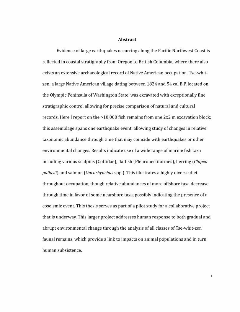
Abstract

Evidence of large earthquakes occurring along the Pacific Northwest Coast is

reflected in coastal stratigraphy from Oregon to British Columbia, where there also

exists an extensive archaeological record of Native American occupation. Tse-whit-

zen, a large Native American village dating between 1824 and 54 cal B.P. located on

the Olympic Peninsula of Washington State, was excavated with exceptionally fine

stratigraphic control allowing for precise comparison of natural and cultural

records. Here I report on the >10,000 fish remains from one 2x2 m excavation block;

this assemblage spans one earthquake event, allowing study of changes in relative

taxonomic abundance through time that may coincide with earthquakes or other

environmental changes. Results indicate use of a wide range of marine fish taxa

including various sculpins (Cottidae), flatfish (Pleuronectiformes), herring (Clupea

pallasii) and salmon (Oncorhynchus spp.). This illustrates a highly diverse diet

throughout occupation, though relative abundances of more offshore taxa decrease

through time in favor of some nearshore taxa, possibly indicating the presence of a

coseismic event. This thesis serves as part of a pilot study for a collaborative project

that is underway. This larger project addresses human response to both gradual and

abrupt environmental change through the analysis of all classes of Tse-whit-zen

faunal remains, which provide a link to impacts on animal populations and in turn

human subsistence.

ii

Acknowledgments

This thesis has been a communal effort to prepare and produce rather than

an individual undertaking. To that end, I have many people to thank for their

support and guidance. First and foremost, I would like to thank the Lower Elwha

Klallam Tribe for their support of this project. Without them, this work would not be

possible. I would like to thank Dr. Laura Phillips at the Burke Museum in Seattle

helping with logistics throughout the project. I would like to thank Dr. Doug Kennett

and Brendan Culleton at UC-Irvine for running the radiocarbon dates for the pilot

study, and to Anna Kagley, Anne Shaffer and Si Simonstad for background

information on local fishes. Thank you Ross Smith and Bob Kopperl for the use of

your comparative fish skeletons. Thank you to the NSF and the PSU Faculty

enhancement grant for funding the pilot study, and thank you to the Association for

Washington Archaeology’s student research grant for helping me purchase software

vital to this work.

Thank you to my friends, cohort members and colleagues. The support and

willingness to commiserate and discuss the trials of graduate school over a good

Portland beer will be cherished. I’d especially like to thank Tony Hofkamp for all of

his help and enthusiasm in identifying bones, rescreening, and providing hours of

entertaining discussion in that windowless lab.

To Dr. Sarah Sterling, whose intimate knowledge of this site and how to

navigate the site report has been extremely valuable; thank you. I’d like to thank Dr.

Shelby Anderson, one of my committee members who graciously stepped in at the

iii

last minute. Your support and insightful comments on work leading up to and

including this thesis have been extremely helpful. I’d like to thank Dr. Kenneth Ames,

a member of my thesis committee and an important mentor to me throughout my

grad school career. He has given me tremendous guidance and helpful, albeit well-

pointed, critique on many class papers that have helped develop this thesis. Ken,

thank you for reminding me to breathe. I would especially like to thank Dr. Virginia

Butler, my amazing advisor. Without her, I would have never been able to accomplish

this thesis. Her enthusiasm and love of archaeology, as well as her patience and

helpful guidance, have been vital to my success as a graduate student. It has been a

pleasure to work so closely with her for the past three years, especially on the Tse-

whit-zen project.

I’d like to thank my family. Your steadfast support has been overwhelming

through this process. I especially thank you for providing a sounding board for ideas,

worries, fears and frustrations. Finally, I’d like to thank my dogs: Brodie and Riley.

Without your unconditional love and cuddles at the end of the day, I surely would

have lost my mind long ago.

iv

Table of Contents

Abstract ...................................................................................................................................................... i

Acknowledgements .............................................................................................................................. ii

List of Tables .......................................................................................................................................... vi

List of Figures ........................................................................................................................................ vii

I. Introduction ........................................................................................................................................ 1

II. Background ....................................................................................................................................... 7

CSZ Environmental Overview 7

Tse-whit-zen in Cultural Context 9

Abrupt Environmental Change and Marine Resources 10

Archaeological Evidence 15

The Value of the Tse-whit-zen Site 19

Environmental Setting of Tse-whit-zen 20

Excavation of Tse-whit-zen 22

Taxonomic Identification Issues 29

III. Methods and Materials .............................................................................................................. 34

Initial Documentation and Processing 34

Analysis 35

IV. Results ................................................................................................................................................ 42

Descriptive Summary of Fish Remains 43

Quantification: NISP and MAU 63

Sample Size 66

Mesh Size 68

Tse-whit-zen Fish Assemblage 69

V. Discussion ........................................................................................................................................... 80

Expectations 80

Habitat Assignment 82

Change over Time in Habitat Use 86

The Impacts of a CSZ Coseismic Event on the Fish and Fisheries of

Tse-whit-zen 91

IV. Conclusions and Future Work................................................................................................... 94

v

Works Cited .......................................................................................................................................... 97

Appendix A: List of possible taxa for the Strait of Juan de Fuca ................................... 107

Appendix B: Comparative collection specimens for the Tse-whit-zen project ....... 109

Appendix C: Elements used to calculate MAU values for each taxon (vertebra counts

from Clothier (1950), Hart (1973), and Butler (1990) ..................................................... 111

vi

List of Tables

Table 3.1

Table of identifiable elements by taxon ..................................................................... 38

Table 4.1

Identified taxa in area A4, Units 17-20 “C” and “CX” bags ................................ 42

Table 4.2

NISP, MAU and Spearman’s ranks for each taxon. Taxa in bold are those with

substantial differences in ranks .................................................................................... 65

Table 4.3

Excavated volume and sample size for “C” bags .................................................... 67

Table 4.4

Taxonomic representation separated by component: “C” bags. Values in bold

are significant at p = .05 ................................................................................................... 73

Table 4.5

Taxonomic representation: comparison of the interior and exterior AZs of the

upper component: “C” bags. Values in bold are significant at p = .05 .......... 76

Table 4.6

Taxonomic representation: comparison of the lower and upper component:

“CX” bags. Values in bold are significant at p = .05 ............................................... 78

Table 5.1

Assignment of fish taxa to habitat ................................................................................ 85

Table 5.2

Distribution of fish in habitat types by AZ. Values in bold are significant at p =

.05 ............................................................................................................................................... 87

vii

List of Figures

Figure 1.1

Cascadia Subduction Zone boundary with site locations (modified and used

with kind permission from the Oregon Department of Geology and Mineral

Industries 1995) ................................................................................................................... 2

Figure 1.2

Regional map showing the location of Port Angeles on the Olympic Peninsula

of Washington State, as well as the location of Tse-whit-zen on the base of

Ediz Hook west of Port Angeles, WA (from Sterling et al. 2011) .................... 4

Figure 2.1

Site map of Tse-whit-zen excavation areas (Reetz et al. 2006, 4-3) .............. 24

Figure 2.2

Area A4 of the Tse-whit-zen excavation with thesis (pilot) units highlighted in

red (Larson 2006) .......................................................................................................... 27

Figure 2.3

Assignment of analytic zones for the 2x2 m pilot unit in Area A4 ................. 29

Figure 4.1

Scatter plot showing significant correlation between logNISP and logMAU

values ........................................................................................................................................ 66

Figure 4.2

“C” bags, the relationship between sample size and excavated volume for each

analytic zone ............................................................................................................... 68

Figure 4.3

Clustered bar chart comparing taxonomic representation of >1/4” mesh

recovery with >1/8” mesh recovery ........................................................................... 69

Figure 4.4

Taxonomic representation for lower and upper component: “C” bags ....... 72

Figure 4.5

Taxonomic representation comparison of upper component interior and

exterior assemblages: “C” bags ...................................................................................... 75

Figure 4.6

Taxonomic representation for lower and upper component: “CX” bags .... 77

viii

Figure 5.1

Designation of habitat types surrounding Tse-whit-zen ................................... 86

Figure 5.2

Distribution of habitat type by analytic zone before and after the occupation

gap: “C” bags .......................................................................................................................... 90

Figure 5.3

Comparison of “CX” bags from lower (bottom) to upper (top) component 91

1

I. Introduction

Project Overview

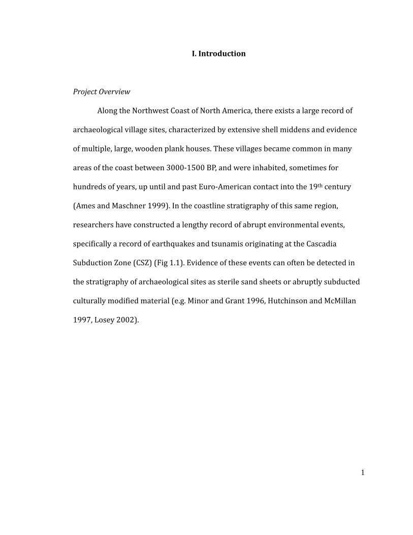
Along the Northwest Coast of North America, there exists a large record of

archaeological village sites, characterized by extensive shell middens and evidence

of multiple, large, wooden plank houses. These villages became common in many

areas of the coast between 3000-1500 BP, and were inhabited, sometimes for

hundreds of years, up until and past Euro-American contact into the 19th century

(Ames and Maschner 1999). In the coastline stratigraphy of this same region,

researchers have constructed a lengthy record of abrupt environmental events,

specifically a record of earthquakes and tsunamis originating at the Cascadia

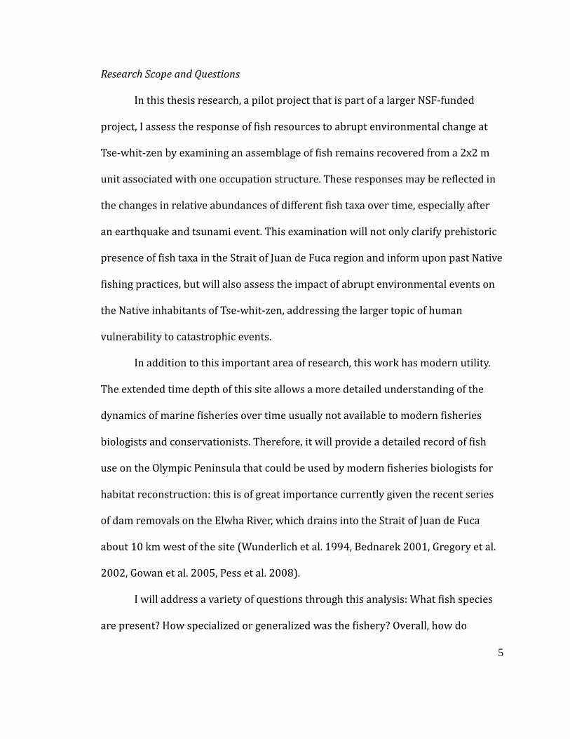
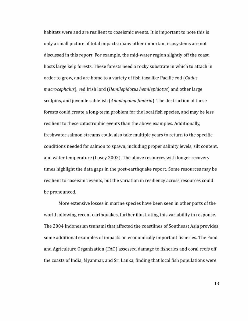
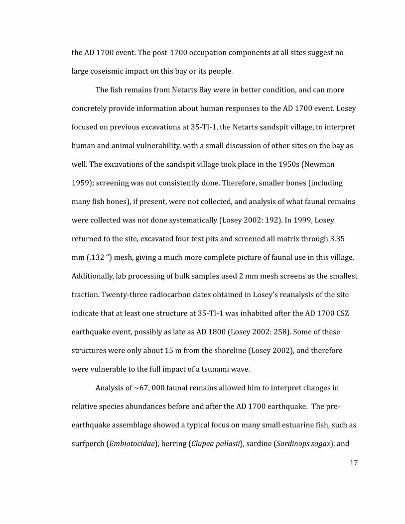
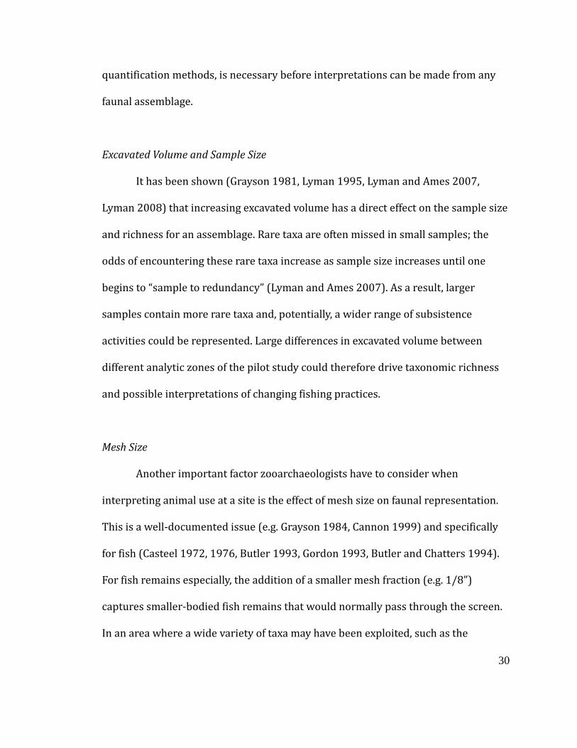
Subduction Zone (CSZ) (Fig 1.1). Evidence of these events can often be detected in

the stratigraphy of archaeological sites as sterile sand sheets or abruptly subducted

culturally modified material (e.g. Minor and Grant 1996, Hutchinson and McMillan

1997, Losey 2002).

Figure 1.1: Cascadia Subduction Zone boundary

and used with kind permission from the Oregon

Mineral Industries 1995

Previous examinations in

communities suffered significant

settlement abandonment after an event (e.g. Hutchinson and

Tveskov and Erlandson 2003

effects of abrupt environmental change. Such evidence has been documented both

in the Northwest Coast region (e.g. Hutchinson and McMillan 1997, Losey 2002,

2005), and worldwide (e.g. papers in Reycraft and Bawden 2000, Goff and McFadgen

2001 and 2003, Stiros 2001, Saltonstall and Carver 2002, Torrence and Grattan

scadia Subduction Zone boundary with site locations

used with kind permission from the Oregon Department of Geology and

1995)

Previous examinations into the archaeology of disaster response

significant stress, community restructuring, and/or

settlement abandonment after an event (e.g. Hutchinson and McMillan 1997,

Tveskov and Erlandson 2003), highlighting the vulnerability of human





2

with site locations (modified

Department of Geology and

the archaeology of disaster response suggest

stress, community restructuring, and/or

lan 1997,

human groups to the





3

2002, Grattan and Torrence 2007). Due to the extended time depth available in the

archaeological record, archaeology is the ideal arena in which to study human

response to abrupt environmental events of the past and the vulnerability and

resilience of coastal societies to these events.

Despite this, documenting human response to catastrophic events

archaeologically is challenging. The coarse resolution of the archaeological record in

most sites prevents the tight linkage of environmental and cultural events, because

of the nature of preservation or excavation techniques (Sterling et al. 2011). Well-

resolved chronologies may exist for environmental events and even cultural

processes such as house construction, but these timelines are difficult to overlay

because they are based on differing time scales. A site with specific qualifications is

necessary to address human response to abrupt environmental change: it must

possess a lengthy occupational history, have a well-resolved temporal sequence

through control over site formation, and be located where several different

catastrophic events could be identified within the stratigraphy.

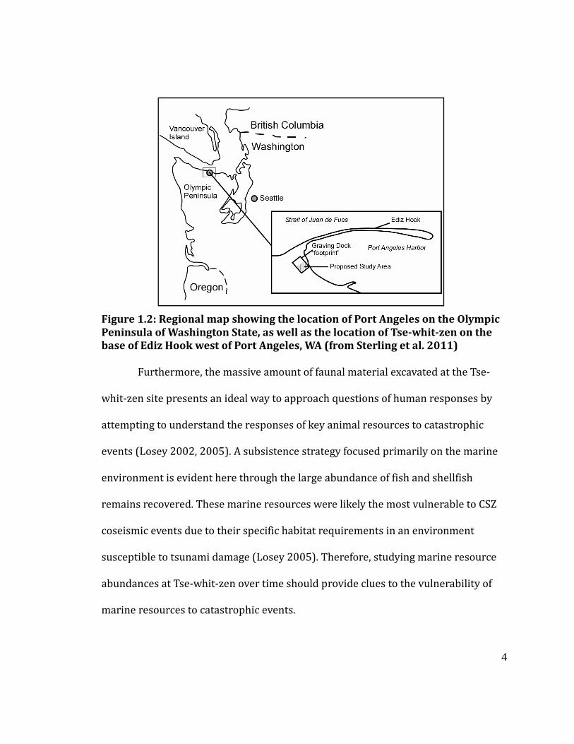
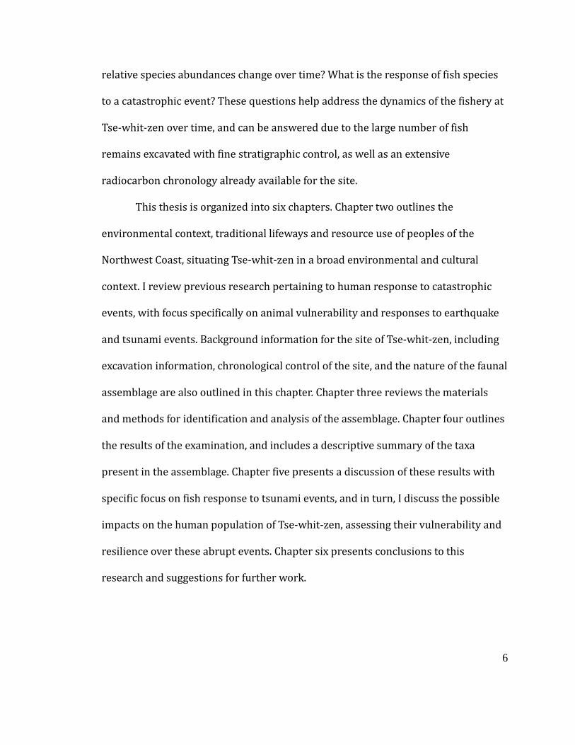
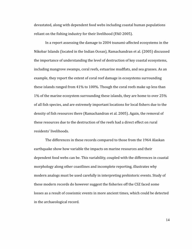
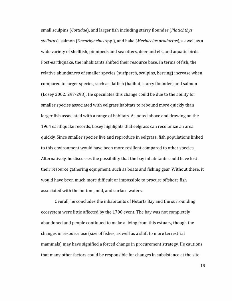
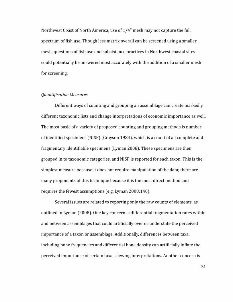
The site of Tse-whit-zen, on the Olympic Peninsula of Washington State, USA,

presents a rare opportunity to study this linkage (Fig 1.2). Several plankhouses

spanning about 2000 years of occupational history were excavated here in 2004.

The site was excavated with fine stratigraphic control, allowing for precise

comparison of the natural and the cultural record. The occupational record spans

four known seismic events (Sterling et al. 2006), presenting an opportunity to

address questions of human response to catastrophic events originating at the CSZ.

4

Figure 1.2: Regional map showing the location of Port Angeles on the Olympic

Peninsula of Washington State, as well as the location of Tse-whit-zen on the

base of Ediz Hook west of Port Angeles, WA (from Sterling et al. 2011)

Furthermore, the massive amount of faunal material excavated at the Tse-

whit-zen site presents an ideal way to approach questions of human responses by

attempting to understand the responses of key animal resources to catastrophic

events (Losey 2002, 2005). A subsistence strategy focused primarily on the marine

environment is evident here through the large abundance of fish and shellfish

remains recovered. These marine resources were likely the most vulnerable to CSZ

coseismic events due to their specific habitat requirements in an environment

susceptible to tsunami damage (Losey 2005). Therefore, studying marine resource

abundances at Tse-whit-zen over time should provide clues to the vulnerability of

marine resources to catastrophic events.

5

Research Scope and Questions

In this thesis research, a pilot project that is part of a larger NSF-funded

project, I assess the response of fish resources to abrupt environmental change at

Tse-whit-zen by examining an assemblage of fish remains recovered from a 2x2 m

unit associated with one occupation structure. These responses may be reflected in

the changes in relative abundances of different fish taxa over time, especially after

an earthquake and tsunami event. This examination will not only clarify prehistoric

presence of fish taxa in the Strait of Juan de Fuca region and inform upon past Native

fishing practices, but will also assess the impact of abrupt environmental events on

the Native inhabitants of Tse-whit-zen, addressing the larger topic of human

vulnerability to catastrophic events.

In addition to this important area of research, this work has modern utility.

The extended time depth of this site allows a more detailed understanding of the

dynamics of marine fisheries over time usually not available to modern fisheries

biologists and conservationists. Therefore, it will provide a detailed record of fish

use on the Olympic Peninsula that could be used by modern fisheries biologists for

habitat reconstruction: this is of great importance currently given the recent series

of dam removals on the Elwha River, which drains into the Strait of Juan de Fuca

about 10 km west of the site (Wunderlich et al. 1994, Bednarek 2001, Gregory et al.

2002, Gowan et al. 2005, Pess et al. 2008).

I will address a variety of questions through this analysis: What fish species

are present? How specialized or generalized was the fishery? Overall, how do

6

relative species abundances change over time? What is the response of fish species

to a catastrophic event? These questions help address the dynamics of the fishery at

Tse-whit-zen over time, and can be answered due to the large number of fish

remains excavated with fine stratigraphic control, as well as an extensive

radiocarbon chronology already available for the site.

This thesis is organized into six chapters. Chapter two outlines the

environmental context, traditional lifeways and resource use of peoples of the

Northwest Coast, situating Tse-whit-zen in a broad environmental and cultural

context. I review previous research pertaining to human response to catastrophic

events, with focus specifically on animal vulnerability and responses to earthquake

and tsunami events. Background information for the site of Tse-whit-zen, including

excavation information, chronological control of the site, and the nature of the faunal

assemblage are also outlined in this chapter. Chapter three reviews the materials

and methods for identification and analysis of the assemblage. Chapter four outlines

the results of the examination, and includes a descriptive summary of the taxa

present in the assemblage. Chapter five presents a discussion of these results with

specific focus on fish response to tsunami events, and in turn, I discuss the possible

impacts on the human population of Tse-whit-zen, assessing their vulnerability and

resilience over these abrupt events. Chapter six presents conclusions to this

research and suggestions for further work.

7

II. Background

CSZ environmental overview

Tse-whit-zen is located on the northern shore of the Olympic Peninsula, on

the western edge of Port Angeles in Washington State, USA (Fig 1.2). This region is

situated along the CSZ (Fig 1.1), where the thin Juan de Fuca plate, located offshore

of Oregon and Washington States and Vancouver Island of British Columbia subducts

underneath the thicker North American plate. This zone spans from the Copper

River delta in Alaska to near Cape Mendocino in California (Atwater 1987, Losey

2002); the plate boundary comes to the surface about 80 km offshore of Washington

(Guidoboni and Ebel 2009).

Until the 1980s, researchers believed the CSZ was aseismic, differentiating it

from other parts of the North American coast (California, Alaska). The first clue that

the CSZ was indeed capable of generating massive earthquakes came from geological

evidence within estuarine sediments in southwest Washington (Atwater 1987).

Since then, researchers have used geological and geophysical evidence from

continental shelf stratigraphy (Adams 1990, Goldfinger et al. 2003), marshes

(Hemphill-Haley 1995), tidal wetlands (Jacoby et al. 1997, Satake et al. 2003,

Peterson et al. 2012), and coastal forests (Benson et al. 2001) to argue for the

cyclical recurrence of great earthquakes (moment magnitude > 7.5), capable of

rupturing much of the CSZ every 500-1000 years (e.g. Atwater 1987, Atwater et al.

2004, Satake and Atwater 2007), over the last 7000 years. Along with more local

8

geomorphological changes, these seismic events may have greatly affected the

landform and human occupants, including structures and toolkits, at Tse-whit-zen

multiple times over the course of occupation (Sterling et al. 2006). Possible impacts

could have included ground shaking, coseismic uplift or subsidence, and/or tsunami

surges scouring the nearshore habitat and inland.

Four great earthquakes have been documented for the Olympic Peninsula

spanning the last 2000 years: Event S, occurring between 1700 and 1500 years ago,

Events U/W, two earthquakes geologists have dated between 1400 and 900 years

ago (Williams 1999), and Event Y, dated to AD 1700 corroborated by Japanese

records of an “orphan” tsunami (Atwater et al. 2005). These events have been

documented repeatedly by evidence from turbidity currents and the presence of

tsunami sands on Southern Vancouver Island and Northern Washington (Sterling et

al. 2006, Peterson et al. 2012). They also overlap with the time period Tse-whit-zen

was occupied, estimated from 1824-54 cal BP. While direct evidence for subsidence

and tsunamis has not been documented at the site, geoarchaeologists at Tse-whit-

zen identified anomalous transgressive episodes in the overall emergent character

of the beach, finding evidence of truncated berms and buried swash deposits on

otherwise stable berm features (Sterling et al. 2006). Additionally, Sterling et al.’s

(2011) study of organic matter, phosphorous, and radiocarbon records suggest

patterning in cultural occupation that correlates with the four great earthquakes.

This evidence strongly suggests the people of Tse-whit-zen, and the resource base

on which they relied, were affected by these events.

9

Tse-whit-zen in Cultural Context

The richness of the marine environment off of the Northwest Coast,

combined with human-driven intensification and storage traditions, allowed this

region to be home to an exceptionally dense population. Archaeological and

ethnographic evidence illustrates the ubiquity of large, coastal villages comprised of

multiple plankhouses (Matson and Coupland 1994, Ames and Maschner 1999)

arrayed all along the coast. Villages were situated on the shoreline, with the houses

arrayed in one or two rows, usually on beach ridges or sandspits (Losey 2002) on a

bay or estuary (Ames and Maschner 1999). This orientation allowed for maximum

use of the marine and nearshore environment, though a reliance on the terrestrial

environment was also variably important in different parts of the coast. Travel and

resource procurement were accomplished primarily by boat (Ames and Maschner

1999, Ames 2002), illustrating the need to invest a large amount of capital in

building and upkeep of this equipment.

In addition to boats, communities invested extensively in technology to

augment the harvest of marine resources (Tveskov and Erlandson 2003) and to take

advantage of short seasonal abundances (e.g. large salmon runs) (Suttles 1990).

Plankhouses were the principal food-storage areas for the residents. Important

dried food sources such as dried salmon and other fish, cured whale, seal, and sea

lion blubber and oil, and dried berries that were vital for winter survival were stored

in the houses (Drucker 1965). Ethnographic and archaeological evidence indicates

that groups including the Makah on the Olympic Peninsula (Swan 1869), the Nuu-

10

chah-nulth on Vancouver Island (Arima 1983, McMillan 1999), and the Coast Salish

on the Salish Sea (Suttles 1974) among many others, all engaged in intensive harvest

of coastal and terrestrial resources, storage, and trade.

Abrupt Environmental Change and Marine Resources

The resilience of the crucial economic resources outlined above would in part

determine the vulnerability of Native communities to abrupt environmental change.

One way to make predictions about the ecological impacts of a coseismic event on

local animal resources is to use recent and/or historic earthquakes in coastal

environments as analogs, though difference in coastal morphology and bathymetry

could create varying tsunami hazard along different parts of the coast (Hutchinson

and McMillan 1997). While effort has been put into studying the immediate effects

of coseismic events on coastal human populations, little attention has been devoted

to understanding long-term ecological changes following an event in the CSZ.

The CSZ has not produced an event since the time of European contact in the

early 1800s, precluding use of historic written records to understand ecological

impacts. Losey (2002, 2005) notes the 1964 Good Friday earthquake that originated

at the Aleutian-Alaskan Subduction zone and affected Prince William Sound and the

area around Anchorage, AK, as the most useful analog to an earthquake originating

at the CSZ since there were many similarities in the overall morphology of the coast

and marine environment. It achieved a 9.2 moment magnitude, generated a massive

tsunami, and caused uplift and subsidence all along the coastline (Losey 2005).

11

Geologists and biologists carried out multiple studies to measure these impacts in

the few years following the event (e.g. National Academy of Sciences 1971).

However, these studies were focused on only a few key economic resources, so the

time required for many resources to fully recover remains poorly understood (Losey

2002, 2005, Saltonstall and Carver 2002).

Immediate impacts on mussels and other bivalves, salmon, and other marine

species were reported, showing relatively minor loss of numbers and habitat.

Considerable attention was focused on economically important pink (Oncorhynchus

gorbuscha) and chum (O. keta) salmon over several years after the event as well.

The earthquake negatively affected these resources, though total loss was relatively

small and some positive impacts were reported also. Salmonids spend a majority of

their adult lives out to sea, far away from any effects of a tsunami (Hart 1973, Losey

2002). Only the group that was congregating in the nearshore environment to run

up natal streams, as well as the salmon eggs and alevins in the streams, would be at

risk during the actual event. Losey (2002) reports one-quarter of a million

salmonids (no species indicated) were estimated to have died during the 1964

event. However, up to 3.6 million salmon spawn in rivers draining Prince William

Sound alone every year (Stanley 1968): the overall loss to the fishery therefore was

minor.

At a smaller geographic scale, the losses were more variable. Losey (2002)

reports that in the years following the event, salmon migration up some streams in

the area dropped between 40% and 98%, though some of these “lost” salmon moved

12

to newly created salmon streams. It is also noteworthy that subsided streams lost

only around 8% of their migrating population. Overall, the 1964 event created some

new habitat for salmonid spawning grounds, and subsided areas did not suffer as

severely (Losey 2002). Since the smaller geographic scale shows severe losses in

some affected areas, however, hunter-gatherers relying on local salmon runs could

have suffered major losses; the impact of the earthquake on these peoples could

have been more profound.

Another study following the 1964 earthquake was conducted to understand

recolonization of eelgrass beds (Zostera spp.), which are a vital aspect of the

nearshore habitat and diet for many ecologically important fishes such as herring

(Clupea pallasii) small species of sculpins (Cottidae), and tomcods (Microgadus

proximus) along the Alaskan shoreline and the CSZ as well (Schultz 1990, Byram

2002). Eelgrass beds colonize muddy sandflats in the lower intertidal to subtidal

areas (Schultz 1990), and therefore would be susceptible to tsunami damage via

scouring. Hanna (1966) reports, however, that eelgrass beds were recolonizing

uplifted areas only a year after the event. Also, Losey (2002) notes that eelgrass beds

lose about 75% of their biomass annually due to grazing and yet rebound. It is likely,

if any eelgrass survived the impacts of the coseismic event, that eelgrass beds in the

CSZ would have rebounded quickly.

This historic record is valuable as a starting point in understanding the

intensity of losses to both fish species and their habitats, but the view from the 1964

post-earthquake studies is that losses would be minimal and fish taxa and their

13

habitats were and are resilient to coseismic events. It is important to note this is

only a small picture of total impacts; many other important ecosystems are not

discussed in this report. For example, the mid-water region slightly off the coast

hosts large kelp forests. These forests need a rocky substrate in which to attach in

order to grow, and are home to a variety of fish taxa like Pacific cod (Gadus

macrocephalus), red Irish lord (Hemilepidotus hemilepidotus) and other large

sculpins, and juvenile sablefish (Anoplopoma fimbria). The destruction of these

forests could create a long-term problem for the local fish species, and may be less

resilient to these catastrophic events than the above examples. Additionally,

freshwater salmon streams could also take multiple years to return to the specific

conditions needed for salmon to spawn, including proper salinity levels, silt content,

and water temperature (Losey 2002). The above resources with longer recovery

times highlight the data gaps in the post-earthquake report. Some resources may be

resilient to coseismic events, but the variation in resiliency across resources could

be pronounced.

More extensive losses in marine species have been seen in other parts of the

world following recent earthquakes, further illustrating this variability in response.

The 2004 Indonesian tsunami that affected the coastlines of Southeast Asia provides

some additional examples of impacts on economically important fisheries. The Food

and Agriculture Organization (FAO) assessed damage to fisheries and coral reefs off

the coasts of India, Myanmar, and Sri Lanka, finding that local fish populations were

14

devastated, along with dependent food webs including coastal human populations

reliant on the fishing industry for their livelihood (FAO 2005).

In a report assessing the damage to 2004 tsunami-affected ecosystems in the

Nikobar Islands (located in the Indian Ocean), Ramachandran et al. (2005) discussed

the importance of understanding the level of destruction of key coastal ecosystems,

including mangrove swamps, coral reefs, estuarine mudflats, and sea grasses. As an

example, they report the extent of coral reef damage in ecosystems surrounding

these islands ranged from 41% to 100%. Though the coral reefs make up less than

1% of the marine ecosystem surrounding these islands, they are home to over 25%

of all fish species, and are extremely important locations for local fishers due to the

density of fish resources there (Ramachandran et al. 2005). Again, the removal of

these resources due to the destruction of the reefs had a direct effect on rural

residents’ livelihoods.

The differences in these records compared to those from the 1964 Alaskan

earthquake show how variable the impacts on marine resources and their

dependent food webs can be. This variability, coupled with the differences in coastal

morphology along other coastlines and incomplete reporting, illustrates why

modern analogs must be used carefully in interpreting prehistoric events. Study of

these modern records do however suggest the fisheries off the CSZ faced some

losses as a result of coseismic events in more ancient times, which could be detected

in the archaeological record.

15

Archaeological evidence

Though the study of human responses to catastrophic events has been

undertaken worldwide (e.g. papers in Reycraft and Bawden 2000, Torrence and

Grattan 2002, Grattan and Torrence 2007), few studies directly address how these

events, including coseismic events, would have affected animal populations and

other subsistence resources. Robert Losey’s (2002) study of the vulnerability of the

Tillamook people to the AD 1700 coseismic event is one of the few that directly uses

zooarchaeological evidence linked with tsunami deposits to study marine resource

vulnerability and in turn human responses. Often, changes in resource use are

assumed as part of the human response to coseismic events (Goff and McFadgen

2003, Losey 2005).

In order to interpret human and animal vulnerability on the Oregon coast to

the most recent CSZ earthquake event, Losey (2002, 2005) used the 1964 Good

Friday earthquake as an analog. He also used previous and current archaeological

excavations on two different areas of the coast, Netarts and Nehalem Bays (Fig 1.1),

which were inhabited by the Tillamook people, to assess human and animal

vulnerability and resilience to these events. The results and interpretations from

Losey’s study served as a model for developing my archaeological expectations.

Losey (2002) analyzed numerous previously excavated sites in Nehalem Bay,

including the Cronin Point site (35-TI-4), the Spruce Tree site (35-TI-75), and the

North Trail House site (35-TI-76). All of these sites were initially excavated in the

1980s (Woodward 1986), and were described in very little detail; little is known

16

about the nature of the faunal collections from these excavations. Losey returned to

all three locales and conducted further testing to relocate and map the sites,

excavate test units to collect more cultural material, and gather samples for

radiocarbon dates (Losey 2002). He studied fish remains from contexts dating

before and after the AD 1700 coseismic event. The sample sizes were small and in

very poor condition; Losey reports that the excavated assemblages were comprised

mostly of salmon vertebral fragments. Indeed, the only identifiable bones in the

entire assemblage were salmon vertebrae, suggesting that this assemblage does not

reflect the full spectrum of animal use in this bay. All bone material was fragmented

and chalky (Losey 2002: 528). In these conditions, small-bodied fish bones could

have degraded much more quickly than larger salmon vertebrae. Furthermore,

salmon can be over-represented in assemblages because their vertebrae are easily

identifiable, even if highly fragmented (Casteel 1976: 90-92). These factors could

have led to a bias in the assemblage toward salmonids.

Losey's fish analysis at Nehalem Bay is limited therefore to salmonids, which

he claims suffered a minor impact from the AD 1700 earthquake. The change

through time of fish use can be tracked at the North Trail House site alone because it

is the only site of the three that has a clear pre-1700 occupation component. This

site shows no obvious gap in occupation, and the resource base does not appear to

have shifted greatly. He found, through radiocarbon dating and presence of 19th

century artifacts, that all three Nehalem Bay sites show evidence of occupation after

17

the AD 1700 event. The post-1700 occupation components at all sites suggest no

large coseismic impact on this bay or its people.

The fish remains from Netarts Bay were in better condition, and can more

concretely provide information about human responses to the AD 1700 event. Losey

focused on previous excavations at 35-TI-1, the Netarts sandspit village, to interpret

human and animal vulnerability, with a small discussion of other sites on the bay as

well. The excavations of the sandspit village took place in the 1950s (Newman

1959); screening was not consistently done. Therefore, smaller bones (including

many fish bones), if present, were not collected, and analysis of what faunal remains

were collected was not done systematically (Losey 2002: 192). In 1999, Losey

returned to the site, excavated four test pits and screened all matrix through 3.35

mm (.132 “) mesh, giving a much more complete picture of faunal use in this village.

Additionally, lab processing of bulk samples used 2 mm mesh screens as the smallest

fraction. Twenty-three radiocarbon dates obtained in Losey's reanalysis of the site

indicate that at least one structure at 35-TI-1 was inhabited after the AD 1700 CSZ

earthquake event, possibly as late as AD 1800 (Losey 2002: 258). Some of these

structures were only about 15 m from the shoreline (Losey 2002), and therefore

were vulnerable to the full impact of a tsunami wave.

Analysis of ~67, 000 faunal remains allowed him to interpret changes in

relative species abundances before and after the AD 1700 earthquake. The pre-

earthquake assemblage showed a typical focus on many small estuarine fish, such as

surfperch (Embiotocidae), herring (Clupea pallasii), sardine (Sardinops sagax), and

18

small sculpins (Cottidae), and larger fish including starry flounder (Platichthys

stellatus), salmon (Oncorhynchus spp.), and hake (Merluccius productus), as well as a

wide variety of shellfish, pinnipeds and sea otters, deer and elk, and aquatic birds.

Post-earthquake, the inhabitants shifted their resource base. In terms of fish, the

relative abundances of smaller species (surfperch, sculpins, herring) increase when

compared to larger species, such as flatfish (halibut, starry flounder) and salmon

(Losey 2002: 297-298). He speculates this change could be due to the ability for

smaller species associated with eelgrass habitats to rebound more quickly than

larger fish associated with a range of habitats. As noted above and drawing on the

1964 earthquake records, Losey highlights that eelgrass can recolonize an area

quickly. Since smaller species live and reproduce in eelgrass, fish populations linked

to this environment would have been more resilient compared to other species.

Alternatively, he discusses the possibility that the bay inhabitants could have lost

their resource gathering equipment, such as boats and fishing gear. Without these, it

would have been much more difficult or impossible to procure offshore fish

associated with the bottom, mid, and surface waters.

Overall, he concludes the inhabitants of Netarts Bay and the surrounding

ecosystem were little affected by the 1700 event. The bay was not completely

abandoned and people continued to make a living from this estuary, though the

changes in resource use (size of fishes, as well as a shift to more terrestrial

mammals) may have signified a forced change in procurement strategy. He cautions

that many other factors could be responsible for changes in subsistence at the site

19

that have little to do with coseismic events, but ultimately links the shifts in resource

use he sees to the coseismic event.

Very few case studies of animal response to earthquake events using

zooarchaeology have been carried out, in the Northwest Coast or elsewhere in the

world. The work that has been done highlights that though inhabitants appeared to

live in exposed areas and subsisted on resources that may have been vulnerable to

coseismic impacts, the continuity of occupation at these sites demonstrates some

resilience to coseismic events. However, several limitations to these studies, coupled

with the difficulty of understanding short-term temporal events in the

archaeological record, reinforce the need for more work in this research area. Using

these previous records, I now turn to the village of Tse-whit-zen on the Olympic

Peninsula in order to assess the potential impacts of earthquakes on the aquatic

resources of the Strait of Juan de Fuca.

The Value of the Tse-whit-zen Site

The village of Tse-whit-zen (45CA523) provides a unique opportunity to

assess impacts of abrupt environmental change on the natural resources of the CSZ.

The village site is located in the territory of the Salish speaking Klallam people, and

is a traditional village of the Lower Elwha Klallam Tribe (LEKT). It lies at the

western edge of Port Angeles, Clallam County, Washington, at the base of a sandspit

called Ediz Hook that projects out into the Strait of Juan de Fuca (Fig 1.2). It sits on a

series of beaches that prograded into the bay, now Port Angeles harbor, as the

20

sandspit developed (Sterling et al. 2006). This sandspit facilitated shoreline growth

even after sea level stabilization, which occurred about 5000 years ago, and allowed

the development of sheltered, stable landforms suitable for permanent human

occupation (Sterling et al. 2006). The proximity to the west and southwest of a tidal

marsh and lagoon would have given further access to marine resources, as well as a

sheltered area to store boats, creating an ideal location for a hunter-gatherer village

(Sterling et al. 2006).

While my main goal will be to study fish response to catastrophic events at

Tse-whit-zen, there are several additional benefits to this study as well. My work will

expand our knowledge of Native American fisheries from the Olympic Peninsula

region, providing useful comparisons with fish bone records from the nearby sites of

Hoko River (45CA213) and Ozette (45CA24). Additionally, this data set may assist

current fisheries management and conservation (Moss 2011: 137). For example,

expanded knowledge of the salmon fisheries obtained through this research may aid

salmon habitat restoration and the reestablishment of the large salmon fishery that

should accompany the ongoing removal process of the Elwha River dams

(Wunderlich et al. 1994, Bednarek 2001, Gregory et al. 2002, Gowan et al. 2005, Pess

et al. 2008).

Environmental Setting of Tse-whit-zen

The waters of the CSZ provide an extremely productive environment due to

the prevalence of two atmospheric pressure cells: the North Pacific High and the

21

Aleutian Low (Thomson 1981). In summer, the North Pacific High moves over the

region and causes northwest winds to generate a southbound flow of colder,

Northern Pacific water that collides with the continental shelf and causes an

upwelling of nutrients and oxygen (Thomson 1981). This creates a period of

extreme biological productivity that in turn provides food (e.g. copepods,

zooplankton) to support an abundance of marine life, including a large variety of

pelagic fish species, marine shellfish, sea birds, and sea mammals (Campbell and

Butler 2011). Many of these resources could have been accessed in close vicinity to

Tse-whit-zen.

This large variety of fish resources is found in several habitat types, all of

which could have been accessed by fishers from the village. For example, many

species of bottom-dwelling reef fish live in areas of rocky substrate and kelp forest,

including species of sculpins and Pacific cod (Gadus macrocephalus). More shallow

water, sandy substrate, eelgrass habitat is ideal for smaller species of cottid and

flatfish (Pleuronectiformes). Additionally, species of schooling fish, such as herring,

frequent the nearshore areas seasonally. Offshore and nearshore, larger species,

such as spiny dogfish (Squalus acanthias) are common (Hart 1973). Salmon would

have been available in the Elwha River, ~10 km from the village. Seasonally, five

species of anadromous salmonids migrate up this and other area rivers, providing

massive seasonal abundances that were a staple resource for many coastal groups,

according to both the ethnographic and the archaeological record (e.g. Gunther

1927, Suttles 1990, Huelsbeck and Croes 1980, Campbell and Butler 2011).

22

In addition to these local fish resources, plants, marine shellfish (e.g. mussels

[Mytilus spp.], sea urchin [Strogylocentrotus spp.], chitons [Chitonidae] [Kozloff

1973]), terrestrial (e.g. deer [Odocoileus spp.], elk [Cervus elaphus]), and marine

mammals (e.g. sea lion [Otariidae], harbor seal [Phoca vitulina], sea otter [Enhydra

lutris]) and waterfowl (e.g. multiple species of ducks and geese [Anseriformes],

grebes [Podicipedidae], sandpipers [Scolopacidae]) all played a role in the diet of the

Klallam people (e.g. Croes and Blinman 1980).

Excavation of Tse-whit-zen

The Tse-whit-zen site was excavated as part of the Washington Department

of Transportation (WSDOT) Port Angeles Graving Dock Facility Project. This facility

was intended to provide an area to build large pontoons to aid the replacement of

the Hood Canal Bridge (Larson 2006). After many months of disagreement about the

nature of the site based on the presence of an ethnographic Klallam village near the

area of potential effect (APE) and the discovery of human remains by archaeological

monitors in construction trenches, the Lower Elwha Klallam Tribe (LEKT) and

Larson Anthropological Archaeological Services, Incorporated (LAAS) developed a

field program to delineate site boundaries and determine true significance of this

APE.

WSDOT contracted LAAS to begin a full data recovery excavation in April

2004, which was undertaken by archaeologists from LAAS in close conjunction with

LEKT members. This massive undertaking (Fig 2.1) benefitted from LEKT support

23

and participation; tribal members helped in screening and excavation, as well as

many other areas of the project (Larson 2006, Reetz et al. 2006).

Data recovery was conducted within 1x1 m units grouped into blocks in

order to obtain horizontal exposures and to facilitate the removal of human remains

(Lewarch and Larson 2004). Though the original treatment plan estimated

excavating about 6% of an estimated 2913 m3 cultural material, the actual

excavation removed about 4% of the 6900 m3 revised estimated site volume, 261.4

m3.

Excavation was undertaken following natural strata and was only subdivided

into 10 cm arbitrary levels when the stratum exceeded this thickness. In a single

block, when possible, archaeologists excavated down to the same stratigraphic level

or elevation in order to expose a common surface. This was necessary in order to

establish contemporaneity of different features, of which over 1400 were excavated

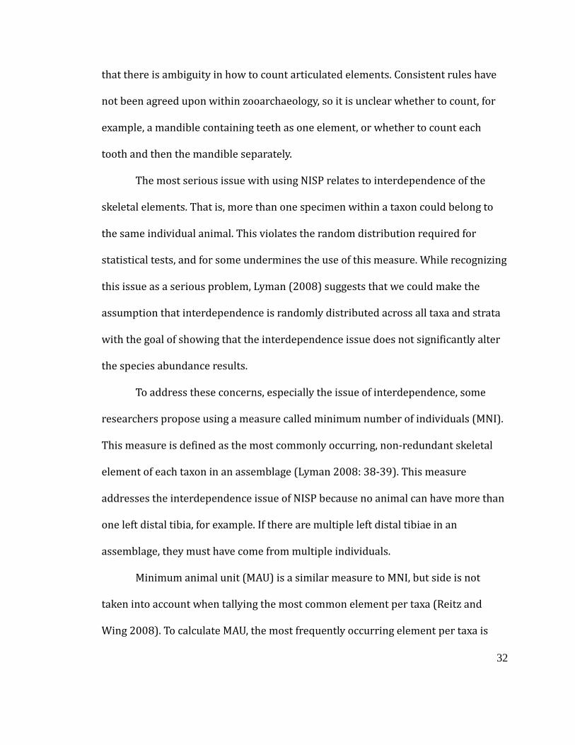
(Larson 2006). Seven major stratigraphic units were identified (Reetz et al. 2006:4-

30). The strata labeled 3 and 5 were the major occupation matrix comprised of

archaeological midden deposits. Strata labeled 6 and 7 were the underlying beach

sands that provided a foundation for the village occupation.

Figure 2.1: Site map of Tse: Site map of Tse-whit-zen excavation areas (Reetz et al. 2006, 4

24

Reetz et al. 2006, 4-3)

25

In order to estimate volume and set aside a sample for studying all faunal

taxa, excavated matrix was placed in 10 L buckets and then brought to the water

screening station. Every 20th 10 L bucket from a given stratum was marked as a

“complete” bucket. The water screening station used a series of nested screens; all

material was deposited in the 1” screen and subsequently screened through

1/2”,1/4”, and 1/8” screen size fractions as well. Problems with the screening

process were discovered later, however, and are discussed below. Use of fine mesh

screens such as 1/8” (or even smaller), is ideal for recovering a representative

sample of faunal material, including small-bodied fish such as herring (e.g. Casteel

1972, 1976, Partlow 2006).

In December 2004, because of the excavation of over 300 intact burials and

archaeological costs soaring over budget, WSDOT decided to stop work at the site in

favor of finding a new location for the graving dock facility. Only preliminary

laboratory sorting was accomplished to separate classes of materials (e.g. lithics,

modified bone, non-human bone) due to the abrupt ending of the project.

My thesis is focused on one 2x2m unit in Area A4 (Fig 2.2), a section of Area

A, which had an estimated site volume of 1900 m3; the largest area excavated in the

site (Reetz et al. 2006). The excavation area of Area A was about 35 x 93 m; 80% of

this area was undisturbed and held intact burials. This area held a rich array of

structural and thermal features, fishing gear, and massive abundances of faunal

material (Reetz et al. 2006:4-31).

26

In order to establish methodology and protocols for the larger NSF project, a

pilot study was developed which represents my thesis research. This unit was

chosen because the cultural layer in A4, associated with Structure 1, was thicker

than anywhere else in the site, with a maximum thickness of 147 cm, encompassing

1800 years of occupation based on 19 14C dates (1824-252 cal years BP) (Reetz et al.

2004:4-38). This unit was also selected because it yielded large samples of each

class of faunal material, which would provide the opportunity to compare analytic

results across faunal classes before undertaking the NSF project.

Figure 2.2: Area A4 of the Tse

highlighted in red (Larson

Seven analytic zones

based on analysis of depositional contexts and stratigraphic relationships (Fig 2.3)

(Sterling et al. 2013). The lower component

by three terminal surfaces

during excavation as strata thought to represent living floors due to their dense

compaction. A palimpsest of cultural material including fish bone, shell,

of the Tse-whit-zen excavation with thesis (pilot) units

ighted in red (Larson 2006)

Seven analytic zones have been defined for this 2x2 m unit (Units 17

analysis of depositional contexts and stratigraphic relationships (Fig 2.3)

The lower component is separated into three zones, identified

terminal surfaces (A4.07, A4.06, A4.05). Terminal surfaces were defined


compaction. A palimpsest of cultural material including fish bone, shell,

27

zen excavation with thesis (pilot) units

(Units 17-20)

analysis of depositional contexts and stratigraphic relationships (Fig 2.3)

zones, identified

Terminal surfaces were defined


compaction. A palimpsest of cultural material including fish bone, shell, charcoal and

28

other material reflected long-term use of the floors, and were used to infer the

presence of structures (Sterling et al. 2006: 7-12). The upper component represents

the presence of Structure 1, and is broken into two contexts. The upper component

of units 17 and 19 is associated with an entry way of the structure, while units 18

and 20 are situated exterior to the structure. This difference in context is reflected

by a different analytic zone assignment (A4.01 and A4.02: entry way, A4.03 and

A4.04: exterior).

Five radiocarbon dates from the 2x2m unit and adjacent contexts suggest the

lower component dates to between 1000 and 1250 B.P. and the upper component to

520 to 770 B.P. (ages uncalibrated) (Sterling et al. 2013). These dates suggest a

~300 year occupation gap between the two components.

Figure 2.3: Assignment of analytic zones for the 2x2 m pilot unit in Area A

Taxonomic Identification

A central goal of

economic importance of

create a record of subsistence practices and human

and space. Before these interpretations can be made, however,

taphonomy, recovery, and quantification on the assemblage must be understood.

Without this context, it is likely that taxonomic representation and abundance coul

be driven by post-depositional or analytical processes

relationships between humans and animals.

excavated volume and mesh size,

: Assignment of analytic zones for the 2x2 m pilot unit in Area A

Taxonomic Identification Issues

most zooarchaeological study is to characterize the

of different taxa (e.g. Grayson 1984, Lyman 2008

create a record of subsistence practices and human-animal relationships over time

Before these interpretations can be made, however, the effect of


Without this context, it is likely that taxonomic representation and abundance coul

depositional or analytical processes as opposed to actual

nships between humans and animals. Understanding recovery issues such as

excavated volume and mesh size, and the effect of different grouping and

29

: Assignment of analytic zones for the 2x2 m pilot unit in Area A4

characterize the relative

Grayson 1984, Lyman 2008) in order to

animal relationships over time

ffect of


Without this context, it is likely that taxonomic representation and abundance could

as opposed to actual

ecovery issues such as

ping and

520-770 BP

1000-1250

BP

30

quantification methods, is necessary before interpretations can be made from any

faunal assemblage.

Excavated Volume and Sample Size

It has been shown (Grayson 1981, Lyman 1995, Lyman and Ames 2007,

Lyman 2008) that increasing excavated volume has a direct effect on the sample size

and richness for an assemblage. Rare taxa are often missed in small samples; the

odds of encountering these rare taxa increase as sample size increases until one

begins to “sample to redundancy” (Lyman and Ames 2007). As a result, larger

samples contain more rare taxa and, potentially, a wider range of subsistence

activities could be represented. Large differences in excavated volume between

different analytic zones of the pilot study could therefore drive taxonomic richness

and possible interpretations of changing fishing practices.

Mesh Size

Another important factor zooarchaeologists have to consider when

interpreting animal use at a site is the effect of mesh size on faunal representation.

This is a well-documented issue (e.g. Grayson 1984, Cannon 1999) and specifically

for fish (Casteel 1972, 1976, Butler 1993, Gordon 1993, Butler and Chatters 1994).

For fish remains especially, the addition of a smaller mesh fraction (e.g. 1/8”)

captures smaller-bodied fish remains that would normally pass through the screen.

In an area where a wide variety of taxa may have been exploited, such as the

31

Northwest Coast of North America, use of 1/4” mesh may not capture the full

spectrum of fish use. Though less matrix overall can be screened using a smaller

mesh, questions of fish use and subsistence practices in Northwest coastal sites

could potentially be answered most accurately with the addition of a smaller mesh

for screening.

Quantification Measures

Different ways of counting and grouping an assemblage can create markedly

different taxonomic lists and change interpretations of economic importance as well.

The most basic of a variety of proposed counting and grouping methods is number

of identified specimens (NISP) (Grayson 1984), which is a count of all complete and

fragmentary identifiable specimens (Lyman 2008). These specimens are then

grouped in to taxonomic categories, and NISP is reported for each taxon. This is the

simplest measure because it does not require manipulation of the data; there are

many proponents of this technique because it is the most direct method and

requires the fewest assumptions (e.g. Lyman 2008:140).

Several issues are related to reporting only the raw counts of elements, as

outlined in Lyman (2008). One key concern is differential fragmentation rates within

and between assemblages that could artificially over or understate the perceived

importance of a taxon or assemblage. Additionally, differences between taxa,

including bone frequencies and differential bone density can artificially inflate the

perceived importance of certain taxa, skewing interpretations. Another concern is

32

that there is ambiguity in how to count articulated elements. Consistent rules have

not been agreed upon within zooarchaeology, so it is unclear whether to count, for

example, a mandible containing teeth as one element, or whether to count each

tooth and then the mandible separately.

The most serious issue with using NISP relates to interdependence of the

skeletal elements. That is, more than one specimen within a taxon could belong to

the same individual animal. This violates the random distribution required for

statistical tests, and for some undermines the use of this measure. While recognizing

this issue as a serious problem, Lyman (2008) suggests that we could make the

assumption that interdependence is randomly distributed across all taxa and strata

with the goal of showing that the interdependence issue does not significantly alter

the species abundance results.

To address these concerns, especially the issue of interdependence, some

researchers propose using a measure called minimum number of individuals (MNI).

This measure is defined as the most commonly occurring, non-redundant skeletal

element of each taxon in an assemblage (Lyman 2008: 38-39). This measure

addresses the interdependence issue of NISP because no animal can have more than

one left distal tibia, for example. If there are multiple left distal tibiae in an

assemblage, they must have come from multiple individuals.

Minimum animal unit (MAU) is a similar measure to MNI, but side is not

taken into account when tallying the most common element per taxa (Reitz and

Wing 2008). To calculate MAU, the most frequently occurring element per taxa is

33

simply divided by the number of times that occurs in the body. For example, seven

Pacific staghorn sculpin dentaries would have to come from at least four fish, since

two dentaries occur in each individual. To ensure each element is counted only once,

only elements with unique landmarks are used in this calculation. For vertebrae, this

means the notochord opening is present and it is more than half complete.

The main issue with MNI (and MAU) is that it is not a fixed value: it can

change according to how the assemblages are grouped and sorted. That is, more

separations made in the assemblage, between different units for example, will raise

the MAU values. Additionally, differential grouping into aggregates could change the

rank order of the taxa, which could lead to different interpretations of the relative

importance of the taxa. These are serious issues pertaining to repeatability of the

identifications and analysis, since there is such a potential for inter-observer

variation.

Taxonomic abundance information from NISP and MNI/MAU are highly

correlated. Each measure may have serious issues, but according to Grayson (1984),

these quantification methods are measuring a consistent property of the

assemblage. Lyman (2008) suggests using multiple lines of evidence to interpret

assemblages; if NISP and MNI are significantly correlated, the issues pertaining to

either method do not have a large impact on interpreting the nature of the

assemblage.

34

III. Methods and Materials

Initial Documentation and Processing

The fish remains recovered in units 17-20 in block A4, Area A, were

borrowed from the Burke Museum of Natural History in Seattle, WA, and were

transported to the zooarchaeology lab at Portland State University for analysis. As

analysis began, it became apparent that the nested screening technique reported

during the excavation was not consistently used in practice. About half of the catalog

numbers, each linked to one 10 L bucket, did not have a 1/8” screen size fraction.

Additionally, the fish remains within each bag were not sorted to the screen size

recorded on the bag tag. For example, fish remains that were supposed to be from

1/4” mesh contained much larger specimens that should have been captured in the

1/2” mesh, as well as much smaller specimens that should have fallen through to

1/8” mesh. In order to ensure comparability with other Northwest Coast

assemblages, as well as the other faunal classes within this site (bird, invertebrate,

mammal), we rescreened all of the material.

Remains from all separate bags from a given catalog number were screened

through nested screens (1/2”, 1/4”, 1/8” screen size fractions). We then re-bagged

the newly screened material into >1/2”, 1/4”, 1/8” and < 1/8” screen size bags, and

assigned new catalog numbers.

I did not include remains which passed through the 1/8” mesh in my analysis

since it is unclear what proportion of original matrix they represent. Also, as noted

35

above, about half of catalog numbers were missing 1/8” sample fractions to begin

with. When these cataloged remains were rescreened, I only included 1/4'” mesh

materials in analysis. These are referred to as “CX” bags. In my analysis, I distinguish

results from the “C” buckets, including size fractions to 1/8” mesh, from “CX” bags,

which includes >1/4” mesh remains.

After the entire assemblage was rescreened, I performed the analysis with

the help of Anthony Hofkamp. All specimen identifications were checked by me and

ultimately by V. L. Butler before recording. This analysis included remains from 50

buckets. Since each bucket contained 10 L of matrix, my study focused on remains

from 500 L of matrix.

Analysis of Assemblage

In setting up the fish bone analysis, I first created a list of possible taxa. I used

previous faunal analyses in the Salish Sea, Puget Sound, and outer coast of

Vancouver Island (Friedman and Croes 1980, Butler 1987, Huelsbeck

1994,McKechnie 2005) and consulted Pacific fisheries guides and reports (Hart

1973, Eschmeyer et al. 1983) to understand life history of these fishes and narrow

down possible species within each family based on modern distribution. Finally, I

used Miller et al. (1980) MESA (Marine Ecosystems Analysis) report, which

presented results from three years of fish surveys along the Strait of Juan de Fuca for

the Environmental Protection Agency (EPA) and the National Oceanic and

Atmospheric Administration (NOAA). Species were recorded from trolling and

36

seining at multiple sites along the Olympic Peninsula; this local information helped

resolve the seasonal movements of some fish taxa (salmon, herring), as well as the

ubiquity of species in the Strait in modern times. Appendix A presents a list of

possible taxa compiled from these sources. All common marine families, including

the most common species of large families of flatfish (Pleuronectiformes) and

scorpionfishes (Scorpaeniformes), were compiled for the comparative collection. In

order to fill gaps in the collection housed in Butler's zooarchaeology lab at Portland

State University, additional skeletons were borrowed from R. Kopperl and R. Smith.

Appendix B lists the specimens included in the comparative collection for this

project.

Specimens were identified to the finest taxonomic level possible based on

unique morphology and landmarks, using the comparative collections. For each

specimen, I recorded a standard set of information, including provenience (area,

unit, stratum, level), mesh size, taxon and element identification (Table 3.1),

evidence of burning, cultural modification, such as butchering marks, and the

presence/absence of unique landmarks (e.g. Reitz and Wing 2008). Unique

landmarks were defined by identifying a non-repetitive portion of the element (e.g.

articular surface). If that portion was present, we assigned it as having a landmark.

For vertebrae, the presence of the notochord opening in the centrum qualified as

having a landmark (Butler 1993, 1996). We distinguished between abdominal and

caudal vertebrae based on the presence and orientation of the neural and haemal

processes (Wheeler and Jones 1989). Additionally, the last ~5 vertebrae were too

37

similar to distinguish between several families: a “non-salmonid” category was

created to track these “too caudal to identify” vertebrae. Salmon vertebrae are easily

identifiable, even when highly fragmented, and so this “non-salmonid” category was

also used to track the amount of the assemblage that we could not identify to

evaluate the potential bias in salmon identification. I also kept track of unidentified

fish remains (“Unid” fish) in order to track potential differences in identifiably and

fragmentation through time. Identification information was recorded in the

Statistical Package for Social Science (SPSS), Version 21 for analysis.

38

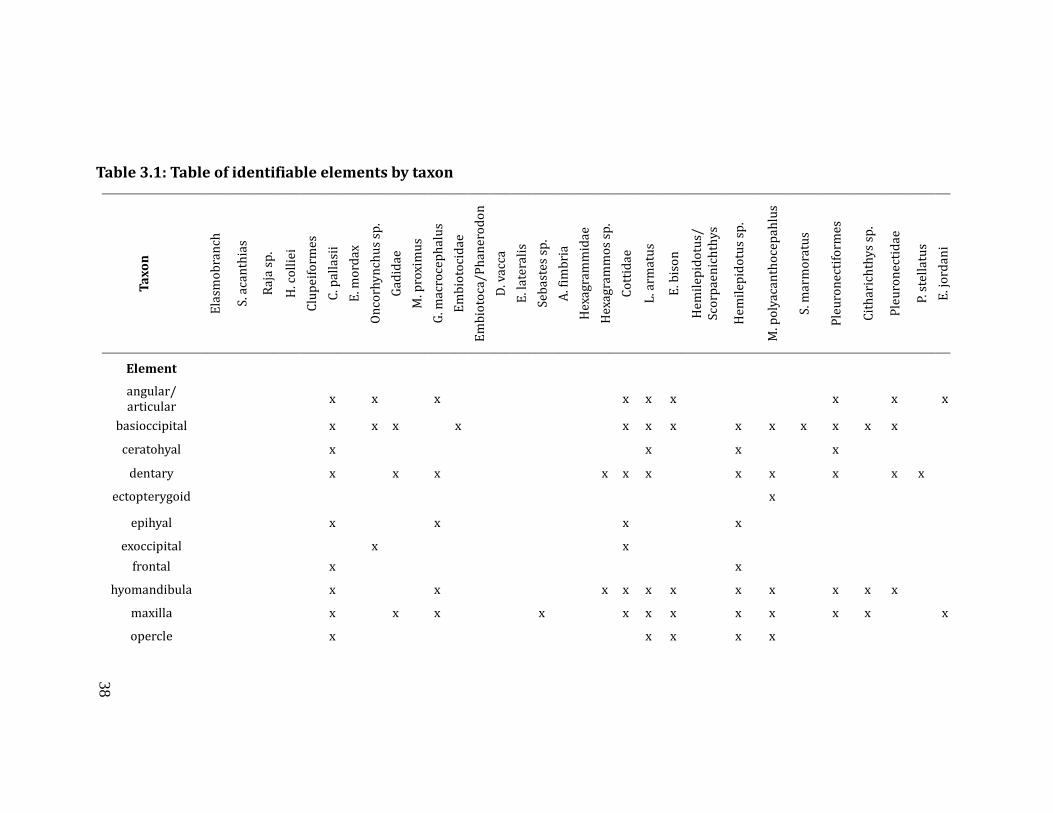
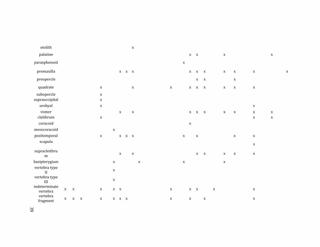
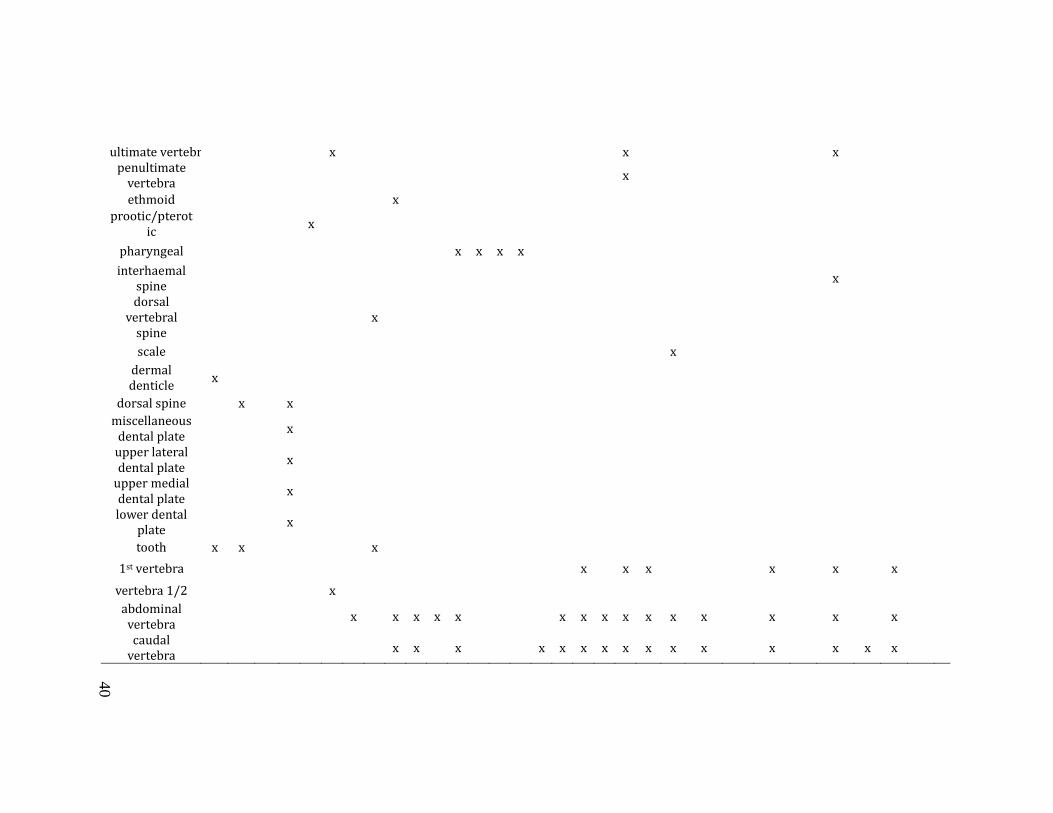
Table 3.1: Table of identifiable elements by taxon

Ta

xo

n

Ela

smo

bra

nch

S. a

can

thia

s

Ra

ja s

p.

H. c

oll

iei

Clu

pe

ifo

rme

s

C. p

all

asi

i

E. m

ord

ax

On

corh

yn

chu

s sp

.

Ga

did

ae

M. p

rox

imu

s

G. m

acr

oce

ph

alu

s

Em

bio

toci

da

e

Em

bio

toca

/P

ha

ne

rod

on

D. v

acc

a

E. l

ate

rali

s

Se

ba

ste

s sp

.

A. f

imb

ria

He

xa

gra

mm

ida

e

He

xa

gra

mm

os

sp.

Co

ttid

ae

L. a

rma

tus

E. b

iso

n

He

mil

ep

ido

tus/

Sco

rpa

en

ich

thy

s

He

mil

ep

ido

tus

sp.

M. p

oly

aca

nth

oce

pa

hlu

s

S. m

arm

ora

tus

Ple

uro

ne

ctif

orm

es

Cit

ha

rich

thy

s sp

.

Ple

uro

ne

ctid

ae

P. s

tell

atu

s

E. j

ord

an

i

Element

angular/

articular x x x x x x x x x

basioccipital x x x x x x x x x x x x x

ceratohyal x x x x

dentary x x x x x x x x x x x

ectopterygoid x

epihyal x x x x

exoccipital x x

frontal x x

hyomandibula x x x x x x x x x x x

maxilla x x x x x x x x x x x x

opercle x x x x x

39

otolith x

palatine x x x x

parasphenoid x

premaxilla x x x x x x x x x x

preopercle x x x

quadrate x x x x x x x x x

subopercle x

supraoccipital x

urohyal x x

vomer x x x x x x x x x

cleithrum x x x

coracoid x

mesocoracoid x

posttemporal x x x x x x x x

scapula

x

supracleithru

m x x x x x x x

basipterygium x x x x

vertebra type

II x

vertebra type

III x

indeterminate

vertebra x x x x x x x x x x

vertebra

fragment x x x x x x x x x x x

40

ultimate vertebra x x x

penultimate

vertebra x

ethmoid x

prootic/pterot

ic x

pharyngeal x x x x

interhaemal

spine x

dorsal

vertebral

spine

x

scale x

dermal

denticle x

dorsal spine x x

miscellaneous

dental plate x

upper lateral

dental plate x

upper medial

dental plate x

lower dental

plate x

tooth x x x

1st vertebra x x x x x x

vertebra 1/2 x

abdominal

vertebra x x x x x x x x x x x x x x x

caudal

vertebra x x x x x x x x x x x x x x x

41

To facilitate comparison with other fish assemblages, I tallied specimens

using both NISP and MAU, as discussed above. I then performed several analyses to

understand the post-depositional history of the assemblage, in order to ensure that

any patterns that emerged were not simply due to taphonomy or recovery

techniques. To begin, I compared the two different quantification methods used

(NISP and MAU) to see if they were measuring similar properties of the assemblage.

I then assessed the effects of different mesh sizes on taxonomic representation, and

the effects of excavated volume on the sample size for each AZ in order to ensure

sample size was not driving taxonomic patterning.

I compared the “C” fish assemblage across AZs to determine the degree of

similarity in fish use over time. I also compared the interior and exterior

assemblages in the upper component to determine if differences in taxonomic

representation existed within the same time period. Finally, I compared the “CX”

assemblage across AZs to track any changes in large-bodied fish use through time

that may have been difficult to interpret in the “C” assemblage.

To test for change over time in the fish assemblage, I grouped the fish taxa into

different habitat types to simplify tracking the large number of different taxa. I then

used a chi square test on the “C” and “CX” assemblages to determine if the fish

represented by the defined habitats were distributed across time. This test shows

whether or not different patterns of fish use exist before and after the occupation

gap that could indicate a CSZ coseismic event.

42

IV. Results

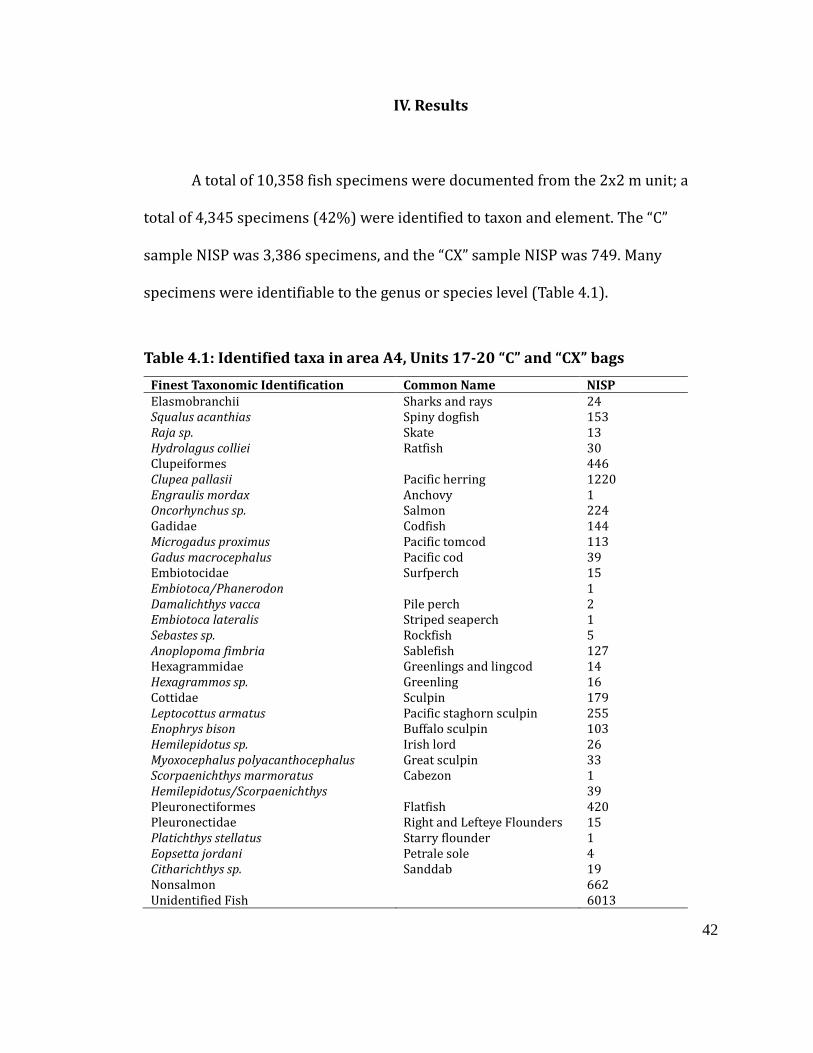
A total of 10,358 fish specimens were documented from the 2x2 m unit; a

total of 4,345 specimens (42%) were identified to taxon and element. The “C”

sample NISP was 3,386 specimens, and the “CX” sample NISP was 749. Many

specimens were identifiable to the genus or species level (Table 4.1).

Table 4.1: Identified taxa in area A4, Units 17-20 “C” and “CX” bags

Finest Taxonomic Identification Common Name NISP

Elasmobranchii Sharks and rays 24

Squalus acanthias Spiny dogfish 153

Raja sp. Skate 13

Hydrolagus colliei Ratfish 30

Clupeiformes 446

Clupea pallasii Pacific herring 1220

Engraulis mordax Anchovy 1

Oncorhynchus sp. Salmon 224

Gadidae Codfish 144

Microgadus proximus Pacific tomcod 113

Gadus macrocephalus Pacific cod 39

Embiotocidae Surfperch 15

Embiotoca/Phanerodon 1

Damalichthys vacca Pile perch 2

Embiotoca lateralis Striped seaperch 1

Sebastes sp. Rockfish 5

Anoplopoma fimbria Sablefish 127

Hexagrammidae Greenlings and lingcod 14

Hexagrammos sp. Greenling 16

Cottidae Sculpin 179

Leptocottus armatus Pacific staghorn sculpin 255

Enophrys bison Buffalo sculpin 103

Hemilepidotus sp. Irish lord 26

Myoxocephalus polyacanthocephalus Great sculpin 33

Scorpaenichthys marmoratus Cabezon 1

Hemilepidotus/Scorpaenichthys 39

Pleuronectiformes Flatfish 420

Pleuronectidae Right and Lefteye Flounders 15

Platichthys stellatus Starry flounder 1

Eopsetta jordani Petrale sole 4

Citharichthys sp. Sanddab 19

Nonsalmon 662

Unidentified Fish 6013

43

Descriptive Summary of Fish Remains

The following section describes criteria used for specimen identification.

When necessary, I have included features used to distinguish closely related species.

Information on range, habitat, and modern distribution is included as well.

Class Chondrichthys – cartilaginous fishes

Subclass Elasmobranchii – sharks and rays

Material: 1 indeterminate vertebra, 8 vertebral fragments, 11 dermal denticles, 4

teeth: 24 specimens.

Order Squaliformes

Family Squalidae – dogfish sharks

Squalus acanthias – spiny dogfish

Material: 35 indeterminate vertebrae, 121 vertebral fragments, 6 dorsal spines, 1

tooth: 163 specimens.

Order Rajiformes – skates and rays

Family Rajidae - skates

Raja sp.

44

Material: 13 vertebral fragments: 13 specimens.

Remarks: A variety of sharks and rays live in the Northeast Pacific (Hart 1973).

Elements were assigned to the Elasmobranchii category if they were too eroded to

be separated into one family, but still retained the distinctive morphology common

to this class. The teeth, as well as the toothlike scales (Hart 1973), or dermal

denticles, embedded in the skin of sharks and rays vary greatly in size and shape,

making them difficult to separate below the level of subclass. Additionally, the spool

shaped vertebrae, if too eroded to identify the distinctive projecting struts on the

Raja vertebrae, cannot be further separated.

Spiny dogfish is the most common species of small shark in the Northeast

Pacific (Eschmeyer et al. 1983), and the only member of the Squalidae family living

in the study area. They are diverse predators, feeding on many other species found

in this assemblage, and congregate where feeding opportunity is abundant. Hart

(1973) notes these fish are found at depths of up to 400 fathoms (750 m) to the

surface, but are highly migratory and commonly associated with the marine benthos.

The elongate, spool shape of the vertebra, even when broken in the middle,

allowed for positive species level identification. The dorsal spines, located anterior

to the dorsal fin on this species, are distinguishable from those of Hydrolagus colliei

based on the presence of a deep posterior groove, a dark, shiny surface, no serration

45

on the posterior edge, and convex curvature when viewed laterally. Two of these

spines are present on each fish.

Multiple species of the genus Raja (skates) inhabit the study area. Our

comparative collection only contains one species, however (Raja rhina), so these

vertebrae were identified to the genus level. Skate vertebrae are distinct from those

of Squalus acanthias due to their rostro-caudal compression and strong struts that

connect to each margin of the vertebra, forming a star shape when broken in half.

The genus Raja is the only one within the Rajiformes that is common in shallow

water and likely utilized by native fishers. The big skate (Raja binoculata) can reach

lengths of 240 cm (Hart 1973). They are bottom fish that can be found in shallow

water to around 200 fathoms (366 m) (Hart 1973).

Subclass Holocephali

Order Chimaeriformes

Family Chimaeridae - chimaeras

Hydrolagus colliei – spotted ratfish

Material: 2 dorsal spines, 3 miscellaneous dental plates, 9 upper lateral dental

plates, 11 upper medial dental plates, 5 lower dental plates: 30 specimens.

Remarks: Hydrolagus colliei is the only member of the family found in the North

Pacific. They are found in abundance between 50 and 150 fathoms (92-275 m) near

46

shore, but have been taken in catches from up to 499 fathoms (913 m) (Hart 1973).

They are a common visitor to shallow waters (Hart 1973). In the Strait of Juan de

Fuca MESA near shore fish report, Miller et al. (1980) report capture of these fish

both with tow net and beach seine methods.

An individual ratfish has six distinctive dental plates: two pairs on the upper

jaw, and one pair on the lower jaw. These teeth are distinctive due to their flat, plate-

like structure, and can be identified by individual teeth. The dorsal spine of ratfish is

distinguished from Squalus acanthias spines because they are not curved, have a

serrated posterior border, and lack a dark, glossy, enamel-like surface. One of these

spines is present on each individual.

Class Osteichthyes – bony fishes

Order Clupeiformes

Material: 610 prootic/pterotic: 610 specimens.

Family Clupeidae – herrings

Clupea pallasii – Pacific herring

Material: 42 angular/articulars, 10 basioccipitals, 73 ceratohyals, 88 dentaries, 32

epihyals, 14 frontals, 2 parietals, 15 hyomandibulae, 38 maxillae, 49 opercles, 25

quadrates, 16 subopercles, 10 supraoccipitals, 1 urohyal, 9 cleithra, 2 posttemporals,

47

1,391 indeterminate vertebrae, 55 vertebral fragments, 14 ultimate

vertebrae/hypurals, 34 1st/2nd vertebrae: 1,920 specimens.

Remarks: Two families comprise the Clupeiformes order: Clupeidae (herrings) and

Engraulidae (anchovies) (Hart 1973). They are both small schooling fish with

seasonal spawning abundances in the Northeast Pacific. Two species of herring are

present in the study area: Clupea pallasii (Pacific herring) and Sardinops sagax

(Pacific sardine).

Prootics and the pterotics are difficult to distinguish to element. Both consist

of a thin, bony plate surrounding a hollow, ball-like structure. As well, these

elements are indistinguishable between Pacific herring and northern anchovy.

Pacific herring alone was identified in the pilot study analysis, so it is likely that all of

the –otics belong to Pacific herring.

A large number of elements were identifiable to the species level due to the

completeness of the archaeological elements and the morphologically distinctive

characteristics of the cranial elements of Pacific herring compared to other

Clupeiformes.

Order Salmoniformes

Family Salmonidae – salmon and trout

Oncorhynchus sp.

48

Material: 1 angular/articular, 1 basioccipital, 1 exoccipital, 1 mesocoracoid, 1

pectoral fin ray, 3 basipterygia, 35 Type 2 vertebrae, 55 Type 3 vertebrae, 7

indeterminate vertebrae, 159 vertebral fragments, 6 dorsal vertebral spines, 2 teeth:

272 specimens.

Remarks: Seven species of anadromous salmon (genus Oncorhynchus) inhabit the

fresh and saltwater habitats of the study area, including O. gorbuscha (pink salmon),

O. keta (chum salmon), O. kisutch (coho salmon), O. nerka (sockeye salmon), O. clarkii

(cutthroat trout), O. mykiss (steelhead) and O. tshawytscha (chinook salmon) (Hart

1973). Though attempts have been made to separate these species using

osteological material, (e.g. Huber et al. 2011), no reliable morphological criteria have

been developed to allow for species level identification of cranial elements,

postcranial elements, or vertebrae. Therefore, all elements were identified to the

genus level. Several elements, including dorsal vertebral spines and the

mesocoracoid, were identified for salmonids alone because of the overall paucity of

salmon remains, likely due to lower bone density (Butler 1990).

Order Gadiformes

Family Gadidae – codfishes

49

Material: 2 basioccipitals, 2 dentaries, 3 maxillae, 1 premaxilla, 3 quadrates, 1 vomer,

1 posttemporal, 2 supracleithra, 3 indeterminate vertebrae, 10 vertebral fragments,

1 ethmoid, 50 abdominal vertebrae, 66 caudal vertebrae: 145 specimens.

Microgadus proximus – Pacific tomcod

Material: 1 premaxilla, 1 posttemporal, 2 vertebral fragments, 4 atlas vertebrae, 91

abdominal vertebrae, 18 caudal vertebrae: 96 specimens.

Gadus macrocephalus – Pacific cod

Material: 1 angular/articular, 2 dentaries, 2 epihyals, 1 hyomandibula, 4 maxillae, 3

otoliths, 9 premaxillae, 3 quadrates, 6 vomers, 4 posttemporals, 4 supracleithra, 1

abdominal vertebra: 40 specimens.

Remarks: Three species of gadid are common in the Northeast Pacific: Pacific cod

(Gadus macrocephalus) walleye pollock (Theragra chalcogramma) and tomcod

(Microgradus proximus) (Hart 1973). Pacific cod can reach lengths of about 1 meter

(Hart 1973). They come together in deeper water to spawn in winter, and move back

to shallow water in the spring. They are mostly benthic, to depths of 300 fathoms

(550 m), but can also be taken in very shallow water. Tomcod, a much smaller fish

than Pacific cod, are found at depths between 15 and 50 fathoms (27-92 m). Walleye

50

pollock can reach lengths to 91 cm, according to Hart (1973), but are often much

smaller than this. They are distributed from surface to below 200 fathoms (366 m)

(Hart 1973).

Many cranial elements retained morphological characteristics that enabled

identification to the species level, especially for Pacific cod. These characteristics

include the shape and tooth placement on the dentary and vomer, the morphology of

the maxillary condyle, the morphology of the quadrate articulation, the ascending

process of the premaxilla, and the morphology of the supracleithrum. Some tomcod

vertebrae were distinctive enough to separate, especially the abdominals, based on

the solid character of the centra. Vertebrae were identified as Pacific cod based on

its extremely large size.

Order Scorpaeniformes

Material: 4 abdominal vertebrae, 6 caudal vertebrae: 10 specimens.

Remarks: This order contains numerous species of rockfish, greenling, and sculpin

that are a variety of sizes and are common in the Northeast Pacific. Their vertebrae

are heavily built and share some similar features. The vertebrae identified only to

the order level were too eroded or broken to identify them to a lower taxonomic

level.

51

Family Anoplopomatidae

Anoplopoma fimbria – Sablefish

Material: 1 quadrate, 13 indeterminate vertebrae, 18 vertebra fragments, 27


Remarks: Two species within this family are represented in the Northeastern

Pacific: Anoplopoma fimbria and Erlipes zonifer. Our archaeological specimens

closely matched Anoplopoma, though we lack reference material for Erlipes zonifer

so the identification is somewhat tentative. Juvenile sablefish move into shallow

water where they would more likely be taken. Adult sablefish and skilfish are

typically found at extremely great depths (200-500 fathoms or 366-915 m) (Hart

1973), much beyond the reach of Native fishing technology.

The walls of vertebra identified as sablefish have a fine, fully fenestrated

texture, and are lighter built than other Scorpaeniformes vertebrae.

Family Scorpaenidae – scorpionfishes and rockfishes

Sebastes sp.

Material: 4 caudal vertebrae: 4 specimens.

52

Remarks: Two genera are included in this family: Sebastes and Sebastolobus. At least

35 Sebastes species inhabit the Northeast Pacific (Hart 1973). Two species of

Sebastolobus are also present in the study area, but are morphologically distinct

from Sebastes. According to Miller et al. (1980), three species of rockfish were

captured in beach seine and tow net catches during three years of surveying the

Strait of Juan de Fuca. Scorpaenids can be found in many different habitats,

including bays, kelp beds, and along the shore (Eschmeyer et al. 1983) and from the

intertidal to depths of up to 2800 meters (Hart 1973).

Family Hexagrammidae – greenlings and lingcods

Material: 1 atlas vertebra, 1 abdominal vertebra, 9 caudal vertebrae: 11 specimens.

Hexagrammos sp. - greenlings

Material: 1 dentary, 2 hyomandibulae, 1 basipterygium, 1 abdominal vertebra, 3

caudal vertebrae: 8 specimens.

Remarks: Hexagrammids are a small family of elongate bottom fish, including the

lingcod (Ophiodon elongatus), and four species of greenling (Hexagrammos sp.) in

the Northeast Pacific (Hart 1973). Two other genera are in this family, each

including one species in the northern Pacific: the painted greenling (Oxylebius

53

pictus) and the atka mackerel (Pleurogrammus monopterygius) (Eschmeyer et al.

1983). We identified Hexagrammos remains based on an extremely close match to

the comparative specimens. However, since we do not have Oxylebius or

Pleurogrammus in the reference collection, this identification is tentative. The beach

seine and tow net surveys of the Strait of Juan de Fuca collected specimens of kelp,

rock, and whitespotted greenling as well as lingcod, but not painted greenling or

atka mackerel (Miller et al. 1980).

Greenlings are common in shallow water along rocky shores, but lingcod are

found to 230 fathoms (421 m). They are most commonly distributed in the upper 50

fathoms (92 m) off the coast in the Northeast Pacific (Hart 1973).

Family Cottidae – sculpins

Material: 3 angular/articulars, 6 basioccipitals, 9 dentaries, 1 epihyal, 1 exoccipital, 3

hyomandibulas, 1 maxilla, 1 palatine, 4 premaxillae, 6 quadrates, 2 vomers, 1

coracoid, 1 indeterminate vertebra, 2 vertebral fragments, 3 ultimate

vertebrae/hypurals, 1 penultimate vertebra, 4 atlases, 46 abdominal vertebrae, 110

caudal vertebrae: 205 specimens.

Leptocottus armatus – Pacific staghorn sculpin

54

Material: 11 angular/articulars, 7 basioccipitals, 3 ceratohyals, 5 dentaries, 12

hyomandibulae, 3 maxillae, 3 opercles, 10 palatines, 3 premaxillae, 2 preopercles, 20

quadrates, 6 vomers, 9 posttemporals, 3 supracleithra, 2 indeterminate vertebrae, 4

atlas vertebrae, 37 abdominal vertebrae, 127 caudal vertebrae: 267 specimens.

Enophrys bison – buffalo sculpin

Material: 1 angular/articular, 3 basioccipitals, 1 hyomandibula, 1 maxilla, 8 opercles,

2 premaxillae, 6 preopercles, 1 quadrate, 2 vomers, 6 supracleithra, 4 vertebral

fragments, 40 lateral line scales, 3 abdominal vertebrae, 27 caudal vertebrae: 105

specimens.

Myoxocephalus polyacanthocephalus - great sculpin

Material: 1 basioccipital, 2 dentaries, 3 hyomandibulas, 4 maxillae, 1 opercle, 1

premaxilla, 2 preopercles, 3 quadrates, 2 vomers, 1 posttemporal, 2 supracleithra, 4

atlas vertebrae, 3 abdominal vertebrae, 3 caudal vertebrae: 32 specimens.

Hemilepidotus spp. – Irish lord

55

Material: 1 basioccipital, 1 ceratohyal, 3 dentaries, 1 epihyal, 1 frontal, 1

hyomandibula, 5 maxillae, 2 opercles, 1 palatine, 4 premaxillae, 1 quadrate, 2

vomers, 2 supracleithra, 2 basipterygia: 27 specimens.

Scorpaenichthys marmoratus – cabezon

Material: 1 basioccipital: 1 specimen.

Hemilepidotus spp./Scorpaenichthys sp.

Material: 1 indeterminate vertebra, 8 abdominal vertebrae, 30 caudal vertebrae: 39

specimens.

Remarks: Cottids are a large family of bottom dwelling fish, ranging in size from

approximately five cm up to 99 cm. They are numerous in the northern Pacific,

especially in shallow water (Eschmeyer et al. 1983), and on the rocky bottom in kelp

forests (Hart 1973). Of the approximately 40 species of sculpin inhabiting the study

area, most are extremely small (less than 10 cm long) (Hart 1973). The six species

reported for Tse-whit-zen are the largest common species in the study area: Pacific

staghorn sculpin, buffalo sculpin, red and brown Irish lord, great sculpin, and

cabezon. All species level identifications are based on the completeness of the

archaeological material and the distinctive characteristics separating elements of

56

each species. Specimens that were not matched precisely to one of the available

specimens were identified to the family level.

Cottid vertebrae are distinctive from other families due to the consistent

“sheath” encasing the centrum. While some were identified to the species level, this

sheath allowed separation of all cottid vertebrae. Many of the cranial elements

identified to family level were too eroded or broken to match them to a comparative

specimen, but with morphological features that still identified the elements to the

family level. All toothed elements identified to species level are based on differences

in tooth patch thickness, tooth orientation, and tooth frequency.

Most elements from the Pacific staghorn sculpin possess a distinctive

morphology that allows easy separation from other large cottid species. For

example, the distal preopercle has three or four spines pointing dorsally that

resemble an antler (Eschmeyer et al. 1983). Buffalo sculpin preopercles also have

several spines, as do other taxa, but the orientation and location of these spines

differentiates the preopercles from these two species. Pacific staghorn sculpin

vertebrae are unique and identifiable based on several characteristics, including the

highly fenestrated centrum on the abdominal vertebrae. Additionally, the caudal

vertebrae have several distinctive characteristics, including the orientation of the

neural and haemal spines and the fenestration on the lateral sides of the centrum.

Pacific staghorn sculpin can grow to 46 cm, and are abundant in tide pools and near

shore on sandy bottom to moderate depths (91 m) (Eschmeyer et al. 1983). They

were collected in beach seines in all three years of survey in the Strait of Juan de

57

Fuca, and were very common in collection sites near Tse-whit-zen (Morse Creek and

Dungeness spit) (Miller et al. 1980).

The buffalo sculpin has distinctive bony lateral line scales. These are firmly

identified to species level. Several elements possess a highly rugose surface texture,

especially the preopercle, the supracleithrum, and the opercle. The vertebrae are

distinctive, possessing a solid appearance with little fenestration through much of

the column. Most of the vertebrae do not possess a strong bar running rostro-

caudally, unlike other sculpin vertebrae. Buffalo sculpin are common in rocky and

sandy inshore areas up to 20 m. They are moderately sized, reaching 37 cm

(Eschmeyer et al. 1983), and are common in the Strait of Juan de Fuca and off of

British Columbia (Hart 1973, Miller et al. 1980).

Two species in the genus Hemilepidotus inhabit the study area: the red Irish

lord (Hemilepidotus hemilepidotus) and the brown Irish lord (H. spinosus). The red

Irish lord is common along the inside coast of British Columbia (Hart 1973), and is

present in the Strait of Juan de Fuca as well (Miller et al. 1980). It is the largest (to

51 cm) and most common species in the genus. They can be found in rocky areas

near shore, and from the intertidal to about 30 m. The brown Irish lord is smaller (to

29 cm) and less common in the study area (Hart 1973). Miller et al. (1980) did not

report any in beach seine or tow net along the Strait of Juan de Fuca in three years of

survey. However, the brown Irish lord could have been more abundant pre-European

contact. Since a brown Irish lord comparative specimen was not available for this

58

analysis, all elements matching the red Irish lord were identified to Hemilepidotus

spp., though they are likely elements of the red Irish lord.

The vertebrae of the Irish lord species and the cabezon were

indistinguishable from each other but distinctive from other cottid vertebrae,

leading to the development of the joint category for these vertebrae.

The two largest cottid species in the study area, the great sculpin and the

cabezon, possess distinctive cranial elements. The great sculpin can reach lengths of

76 cm, though Hart (1973) notes larger individuals have been reported. They are

found from the Puget Sound, Washington state north to the Bering Sea, and are

common near shore. They inhabit areas with sand and mud bottom from the

intertidal to 244 m (Eschmeyer et al. 1983).

The cabezon is extremely common throughout its whole range, from Baja

California to near Sitka, Alaska. Adults are at times found in shallow water (1 m).

They can be very large, up to 99 cm (Eschmeyer et al. 1983), though Hart (1973)

reports a maximum length of 76 cm. They are abundant from the intertidal to 76 m,

and are often caught by fisherman and scuba divers (Eschmeyer et al. 1983).

Order Perciformes

Family Embiotocidae – surfperches

Material: 1 basioccipital, 1 basipterygium, 1 lower pharyngeal, 1 atlas vertebra, 12


59

Embiotoca/Phanerodon

Material: 1 lower pharyngeal: 1 specimen.

Damalichthys vacca – pile perch

Material: 2 lower pharyngeals: 2 specimens.

Embiotoca lateralis – striped seaperch

Material: 1 lower pharyngeal: 1 specimen.

Remarks: Nine species of surfperch currently live in the shallow waters of the

northeastern Pacific, though other species that currently live only off the coast of

California could have inhabited more northern waters pre-European contact.

Depending on the species, these fish live inshore, and their habitats vary from living

in the surf of sandy or rocky beaches, in sheltered bays, or near piers, eelgrass beds,

or underwater structures (Eschmeyer et al. 1983). They can be found from the

surface to as deep as 70 fathoms (128 m)(Hart 1973). The pile perch is the largest

of these (up to 44 cm) and common in the study area. The shiner perch

(Cymatogaster aggregata) is the smallest (to about 15 cm) (Hart 1973). Eschmeyer

60

et al. (1983) note that these are abundant throughout their entire range, and can be

easily caught from piers.

The surfperch lower pharyngeal is the only element identifiable to the

species level based on tooth pattern and element morphology. The

Embiotoca/Phanaedron grouping was created because due to breakage, the

pharyngeal was too fragmentary to separate further.

Order Pleuronectiformes – left and righteye flounders

Material: 3 angular/articulars, 6 basioccipitals, 1 ceratohyal, 4 dentaries, 4

hymandibulas, 6 maxillae, 4 premaxillae, 6 quadrates, 4 urohyals, 6 vomers, 4

cleithra, 2 posttemporals, 1 scapula, 2 supracleithra, 5 indeterminate vertebrae, 2

vertebral fragments, 2 ultimate vertebrae/hypurals, 4 interhaemal spines, 10 atlas

vertebrae, 45 abdominal vertebrae, 315 caudal vertebrae: 436 specimens.

Family Bothidae – lefteye flounders

Citharichthys sp.

Material: 1 basioccipital, 5 hyomandibulae, 2 maxillae, 12 caudal vertebrae: 20

specimens.

Family Pleuronectidae – righteye flounders

61

Material: 2 angular/articulars, 1 basioccipital, 1 dentary, 4 hyomandibulas, 1

palatine, 1 vomer, 1 cleithrum, 1 atlas vertebra, 2 abdominal vertebrae, 1 caudal

vertebra: 15 specimens.

Platichthys stellatus – starry flounder

Material: 1 dentary, 1 stellate scale: 2 specimens

Eopsetta jordani – petrale sole

Material: 1 angular/articular, 2 maxillae, 1 premaxilla: 4 specimens.

Remarks: Right (Pleuronectidae) and lefteye (Bothidae) flounders are distinctive in

that they have an asymmetrical cranium, with both eyes located on one side. The

eyed-side is also pigmented, whereas the “blind” side is lighter or white because it is

usually in contact with the bottom. All flatfish are bottom fish, and many bury

themselves in sediment, leaving just their eyes showing (Eschmeyer et al. 1983, Hart

1973).

Skeletally, flatfish have characteristic elements due to the asymmetry of their

crania, but many elements are difficult to distinguish within species or family and

are therefore identified to the order level. Many, but not all, Pleuronectiformes

62

vertebrae have a distinctive “star shape,” made by two transverse processes

radiating dorso-ventrally on either side of the vertebral centrum (Sakamoto 1984).

These are especially visible on most caudal vertebrae. Additionally, the notochord

opening on Pleuronectiformes vertebrae is situated closer to the neural arch, and

the vertebrae are generally oblong dorso-ventrally. A “lined” texture is characteristic

of the lateral bar on the centrum. The abdominal vertebral face displays a distinctive

asymmetry to the notochord opening, and the neural processes are not offset from

the centrum, but directly adjacent. In some families, the atlas vertebra does not have

an articulated neural spine.

Nineteen pleuronectid species inhabit the study area; due to similarity within

this family, few elements were identifiable below the family level. Bothids include

two species in the study area: Citharichthys sordidus (Pacific sanddab) and C.

stigmaeus (speckled sanddab); both are always left-eyed.

Those elements identified as Pleuronectidae were assigned based on minimal

similarity with the sanddab comparative specimens. Pleuronectids attain much

larger sizes (most around 60 cm, some as large as 267 cm) than the bothids,

allowing assignment of very large elements to the family level (Eschmeyer et al.

1983). Several pleuronectid species are common in the study area, including the

starry flounder (Platichthys stellatus) and several sole species (especially Paroprhys

vetulus [English sole] and Psettichthys melanostictus [sand sole]) (Miller et al. 1980).

Other species (e.g. Eopsetta jordani, or petrale sole) are plentiful in the northeastern

Pacific as well, so the above list is not exhaustive (e.g. Hart 1973). These fish range

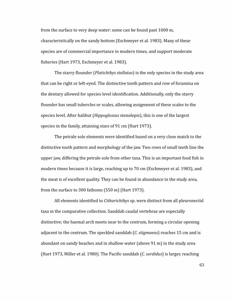
63

from the surface to very deep water: some can be found past 1000 m,

characteristically on the sandy bottom (Eschmeyer et al. 1983). Many of these

species are of commercial importance in modern times, and support moderate

fisheries (Hart 1973, Eschmeyer et al. 1983).

The starry flounder (Platichthys stellatus) is the only species in the study area

that can be right or left-eyed. The distinctive tooth pattern and row of foramina on

the dentary allowed for species level identification. Additionally, only the starry

flounder has small tubercles or scales, allowing assignment of these scales to the

species level. After halibut (Hippoglossus stenolepis), this is one of the largest

species in the family, attaining sizes of 91 cm (Hart 1973).

The petrale sole elements were identified based on a very close match to the

distinctive tooth pattern and morphology of the jaw. Two rows of small teeth line the

upper jaw, differing the petrale sole from other taxa. This is an important food fish in

modern times because it is large, reaching up to 70 cm (Eschmeyer et al. 1983), and

the meat is of excellent quality. They can be found in abundance in the study area,

from the surface to 300 fathoms (550 m) (Hart 1973).

All elements identified to Citharichthys sp. were distinct from all pleuronectid

taxa in the comparative collection. Sanddab caudal vertebrae are especially

distinctive; the haemal arch meets near to the centrum, forming a circular opening

adjacent to the centrum. The speckled sanddab (C. stigmaeus) reaches 15 cm and is

abundant on sandy beaches and in shallow water (above 91 m) in the study area

(Hart 1973, Miller et al. 1980). The Pacific sanddab (C. sordidus) is larger, reaching

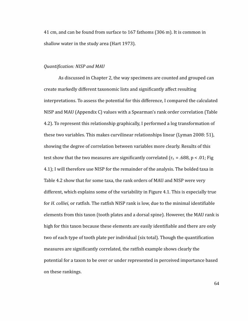
64

41 cm, and can be found from surface to 167 fathoms (306 m). It is common in

shallow water in the study area (Hart 1973).

Quantification: NISP and MAU

As discussed in Chapter 2, the way specimens are counted and grouped can

create markedly different taxonomic lists and significantly affect resulting

interpretations. To assess the potential for this difference, I compared the calculated

NISP and MAU (Appendix C) values with a Spearman’s rank order correlation (Table

4.2). To represent this relationship graphically, I performed a log transformation of

these two variables. This makes curvilinear relationships linear (Lyman 2008: 51),

showing the degree of correlation between variables more clearly. Results of this

test show that the two measures are significantly correlated (rs = .688, p < .01; Fig

4.1); I will therefore use NISP for the remainder of the analysis. The bolded taxa in

Table 4.2 show that for some taxa, the rank orders of MAU and NISP were very

different, which explains some of the variability in Figure 4.1. This is especially true

for H. colliei, or ratfish. The ratfish NISP rank is low, due to the minimal identifiable

elements from this taxon (tooth plates and a dorsal spine). However, the MAU rank is

high for this taxon because these elements are easily identifiable and there are only

two of each type of tooth plate per individual (six total). Though the quantification

measures are significantly correlated, the ratfish example shows clearly the

potential for a taxon to be over or under represented in perceived importance based

on these rankings.

65

Table 4.2: NISP, MAU and Spearman’s ranks for each taxon. Taxa in bold have

substantial differences in ranks Taxon NISP Rank MAU Rank

Squalus acanthias 154 5 3 11

Hydrolagus colliei 30 13 6 3.5

Clupea pallasii 1220 1 112 1

Engraulus mordax 1 25 1 22.5

Onchorhynchus sp. 225 3 3 11

Gadidae 145 6 3 11

Microgadus proximus 114 8 4 7

Gadus macrocephalus 40 10 6 3.5

Hexagrammidae 14 19 1 22.5

Cottidae 179 4 5 5

Sebastes sp. 5 20 1 22.5

Anoplopoma fimbria 127 7 3 11

Hexagrammos sp. 16 18 1 22.5

Leptocottus armatus 255 2 10 2

Enophrys bison 103 9 4 7

Hemilepidotus sp. 27 14 3 11

Myoxocephalus polyacanthocephalus 33 12 4 7

Scorpaenichthys marmoratus 1 25 1 22

Hemilepidotus/Scorpaenichthys 39 11 2 15.5

Embiotocidae 15 16.5 1 22.5

Embiotoca/Phanerodon 1 25 1 22.5

Damalichthys vacca 2 22 2 15.5

Embiotoca lateralis 1 25 1 22.5

Pleuronectidae 15 16.5 2 15.5

Citharichthys sp. 19 15 2 15.5

Platichthys stellatus 1 25 1 22.5

Eopsetta jordani 4 21 1 22.5

Figure 4.1: Scatter plot showing significant correlation between logNISP and

logMAU values.

Sample Size

Patterns in taxonomic representation

volume of excavated matrix increases, assemblages tend to increase in size and

diversity, resulting in a greater NISP value as well as higher taxonomic richness

Lyman and Ames 2007)

use, but they also could simply be due to different recovery methods such as

: Scatter plot showing significant correlation between logNISP and

taxonomic representation can be affected by sample size.


diversity, resulting in a greater NISP value as well as higher taxonomic richness

). These differences can be based on differences in

ut they also could simply be due to different recovery methods such as

66

: Scatter plot showing significant correlation between logNISP and

can be affected by sample size. As the


diversity, resulting in a greater NISP value as well as higher taxonomic richness (e.g.

These differences can be based on differences in animal

ut they also could simply be due to different recovery methods such as

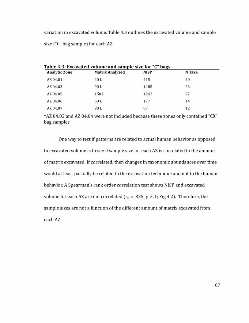
67

variation in excavated volume. Table 4.3 outlines the excavated volume and sample

size (“C” bag sample) for each AZ.

Table 4.3: Excavated volume and sample size for “C” bags Analytic Zone Matrix Analyzed NISP N Taxa

AZ 04.01 40 L 415 20

AZ 04.03 90 L 1485 23

AZ 04.05 150 L 1242 27

AZ 04.06 60 L 177 14

AZ 04.07 90 L 67 12

*AZ 04.02 and AZ 04.04 were not included because these zones only contained “CX”

bag samples

One way to test if patterns are related to actual human behavior as opposed

to excavated volume is to see if sample size for each AZ is correlated to the amount

of matrix excavated. If correlated, then changes in taxonomic abundances over time

would at least partially be related to the excavation technique and not to the human

behavior. A Spearman’s rank order correlation test shows NISP and excavated

volume for each AZ are not correlated (rs = .325, p > .1; Fig 4.2). Therefore, the

sample sizes are not a function of the different amount of matrix excavated from

each AZ.

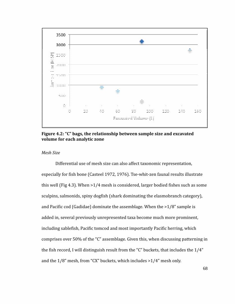
Figure 4.2: “C” bags, the relationship between sample size and excavated

volume for each analytic zone

Mesh Size

Differential use of mesh size can

especially for fish bone (Casteel 1972, 1976

this well (Fig 4.3). When >1/4 mesh is considered,

sculpins, salmonids, spiny dogfish (shark dominating the elasmobranch category),

and Pacific cod (Gadidae) dominate the assemblage. When the >1/8” sample is

added in, several previously unrepresented taxa

including sablefish, Pacific tomcod and most importantly Pacific herring,

comprises over 50% of the “C” assemblage.

the fish record, I will distinguish result from the “C” buckets

and the 1/8” mesh, from “CX” buckets, which includes >1/4”

he relationship between sample size and excavated

for each analytic zone

Differential use of mesh size can also affect taxonomic representation,

fish bone (Casteel 1972, 1976). Tse-whit-zen faunal results illustrate

. When >1/4 mesh is considered, larger bodied fishes



added in, several previously unrepresented taxa become much more prominent

sablefish, Pacific tomcod and most importantly Pacific herring,

% of the “C” assemblage. Given this, when discussing patterning in

the fish record, I will distinguish result from the “C” buckets, that includes the 1/4”

mesh, from “CX” buckets, which includes >1/4” mesh only.

68

he relationship between sample size and excavated

ffect taxonomic representation,

zen faunal results illustrate

larger bodied fishes such as some



become much more prominent,

sablefish, Pacific tomcod and most importantly Pacific herring, which

Given this, when discussing patterning in

, that includes the 1/4”

only.

Figure 4.3: Clustered bar chart

mesh recovery with >1/8” mesh recovery

These issues are important to consider before attempting to

in faunal abundance to actual changes in human or animal behavior. I am

to look for changes over time in the fish record and attribute them more confidently

to human or animal behavior as

The Tse-whit-zen Fish Assemblage

The results of this analysis

time, which is consistent

Croes 1980, Butler 1987

Pacific herring, small cottids

species are common. Species including Pacific cod, s

dogfish are also used commonly

: Clustered bar chart comparing taxonomic representation of >1/4”

mesh recovery with >1/8” mesh recovery

These issues are important to consider before attempting to explain

in faunal abundance to actual changes in human or animal behavior. I am


to human or animal behavior as opposed to taphonomic, recovery or analytic issues.

zen Fish Assemblage

The results of this analysis across AZs show a wide variety of fish use through

which is consistent with information from other area sites (Friedman and

Butler 1987, Huelsbeck 1994, McKechnie 2005). In the “

small cottids (Pacific staghorn sculpin, buffalo sculpin), and flatfish

Species including Pacific cod, salmon, sablefish and spiny

commonly in the site. Perhaps surprisingly, rockfish and

69

comparing taxonomic representation of >1/4”

explain changes

in faunal abundance to actual changes in human or animal behavior. I am now able


or analytic issues.

show a wide variety of fish use through

Friedman and

“C” bag sample,

(Pacific staghorn sculpin, buffalo sculpin), and flatfish

sablefish and spiny

Perhaps surprisingly, rockfish and

70

surfperch are extremely uncommon in this assemblage, and lingcod and plainfin

midshipman are completely absent from this assemblage. These results are

inconsistent with other area site reports, which report larger numbers of these taxa.

The “CX” sample shows a different species composition. Due to the lack of the >1/8”

fraction, Pacific cod, salmon, and spiny dogfish are still common in this sample.

Tracking changes in taxonomic abundances by AZ is one way to assess

changes in fish use over time. Some AZs have very little material in them, so in order

to use them for comparison I combined the upper component AZs (A4.01-A4.04)

and the lower component AZs (A4.05-A4.07) together. Additionally, if a taxon had a

very small sample size (< 5 NISP) I omitted it in order to have an appropriate

assemblage for statistical tests. In all tables below, the categories “small cottid” and

“large cottid” separate the Pacific staghorn sculpin and buffalo sculpin, smaller

cottids found in shallow water (to 12-18”), from the larger cottid species, including

Irish lord, great sculpin, and cabezon. These three taxa are found in deeper water

and attain larger sizes (to 20-30”) (Hart 1973).

I will begin with a comparison of the “C” bag sample, which had large sample

sizes for A4.01 and A4.03, but no material in A4.02 or A4.04, and small samples sizes

in A4.06 and A4.07. Therefore, I combined the AZs into two aggregates. When these

combined lower and upper component assemblages are compared, there is little

change in taxonomic representation: no taxon is present in one component and not

the other.

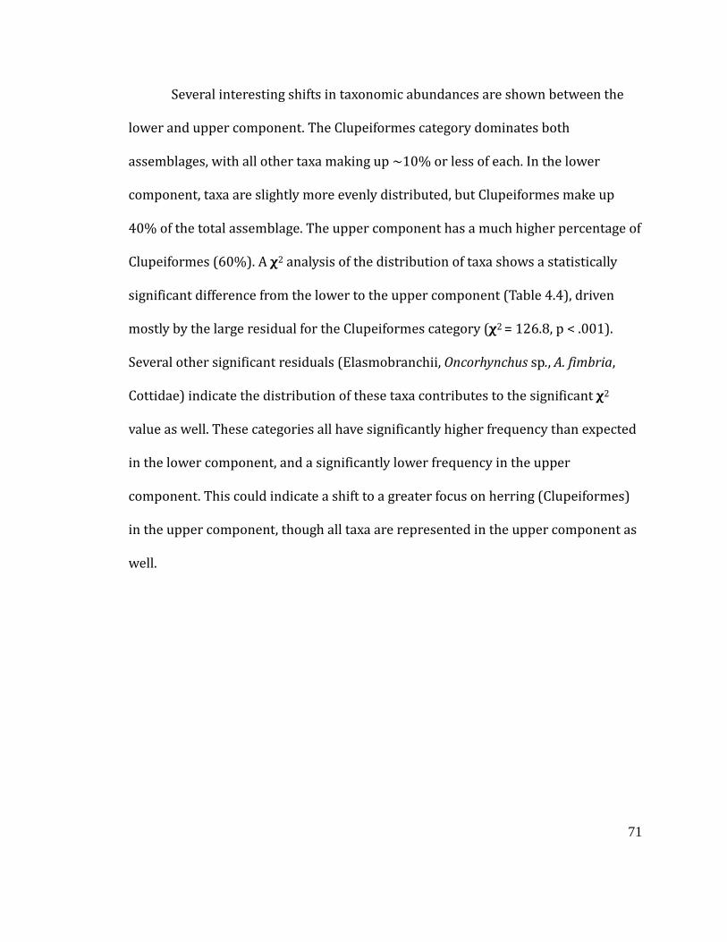
71

Several interesting shifts in taxonomic abundances are shown between the

lower and upper component. The Clupeiformes category dominates both

assemblages, with all other taxa making up ~10% or less of each. In the lower

component, taxa are slightly more evenly distributed, but Clupeiformes make up

40% of the total assemblage. The upper component has a much higher percentage of

Clupeiformes (60%). A χ2 analysis of the distribution of taxa shows a statistically

significant difference from the lower to the upper component (Table 4.4), driven

mostly by the large residual for the Clupeiformes category (χ2 = 126.8, p < .001).

Several other significant residuals (Elasmobranchii, Oncorhynchus sp., A. fimbria,

Cottidae) indicate the distribution of these taxa contributes to the significant χ2

value as well. These categories all have significantly higher frequency than expected

in the lower component, and a significantly lower frequency in the upper

component. This could indicate a shift to a greater focus on herring (Clupeiformes)

in the upper component, though all taxa are represented in the upper component as

well.

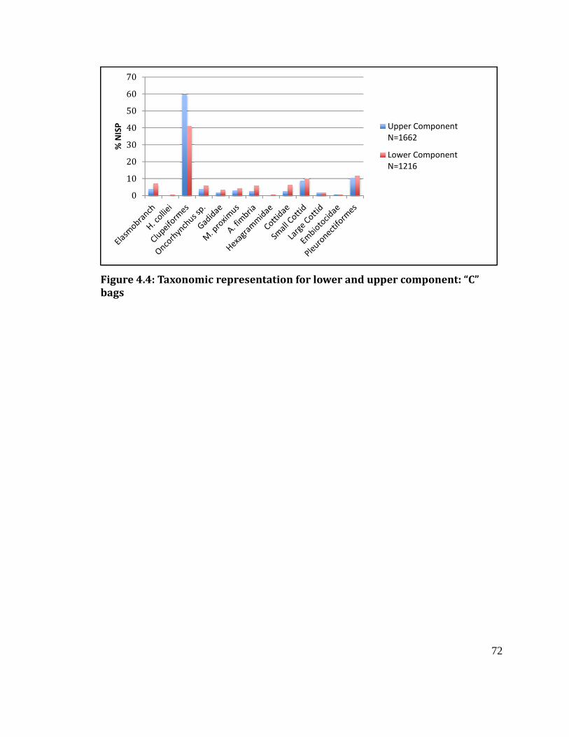
Figure 4.4: Taxonomic representation for lower and upper component: “C”

bags

0

10

20

30

40

50

60

70

% N

ISP


Upper Component

N=1662

Lower Component

N=1216

72


Upper Component

Lower Component

73

Table 4.4: Taxonomic representation separated by component: “C” bags. Values

in bold are significant at p = .05

Finest

Taxa

Common

Name

Upper

Component

Lower

Component

Elasmobranchii Sharks and

Rays

Count 61 87

Expected Count 85.5 62.5

Std. Residual -2.6 3.1

H. colliei Ratfish Count 4 10



Clupeiformes

(dominated by C.

pallasii)

Herring and

Anchovy

Count 995 501


Std. Residual 4.5 -5.2

Oncorhynchus sp. Pacific

Salmon

Count 62 74



Gadidae

(dominated by G.

macrocephalus)

Codfish Count 33 41


Std. Residual 1.5 1.7

M. proximus Pacific

tomcod

Count 52 53


Std. Residual 1.1 1.3

A. fimbria Sablefish Count 46 74



Hexagrammidae Greenling and

lingcod

Count 6 7


Std. Residual -.6 .6

Cottidae Sculpin Count 46 75



Small Cottid Count 149 121



Large Cottid Count 29 21


Std. Residual .0 .0

Embiotocidae Surfperch Count 6 8



Pleuronectiformes Flatfish Count 173 144



74

The upper component is split into an interior context and an exterior midden

context. Here, I compare these two areas to understand the distribution of the fish

bones across the upper component. The sample size from the interior area (A4.01)

is much smaller than that of the exterior, indicating most fish bone in the upper

component is situated outside the structure. This makes sense according to the

ethnographic record of house cleaning and trash disposal (Gunther 1927). The

exterior context is dominated by Clupeiformes (>60% of the assemblage), again with

all other taxa comprising ~10% or less of the assemblage. A χ2 analysis of the

distribution presents a statistically significant result (χ2 = 48.25, p < .001; Table 4.5).

Similar to the previous comparison, Clupeiformes are significantly more common in

the exterior context, but again this category still has a strong presence in both

contexts. Though a variety of taxa are represented, the very large abundance of

Clupeiformes further suggests a focus on these fish in the upper component.

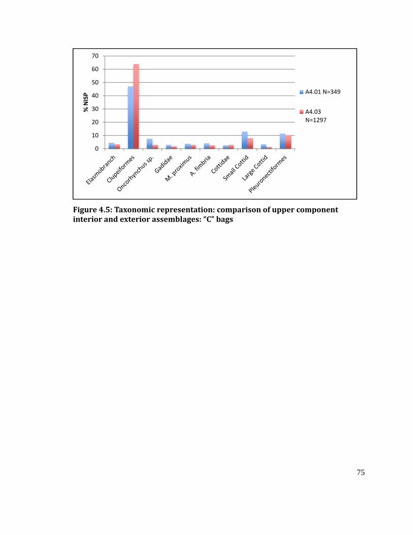
Figure 4.5: Taxonomic representation:

interior and exterior assemblages

0

10

20

30

40

50

60

70

% N

ISP

e 4.5: Taxonomic representation: comparison of upper component

interior and exterior assemblages: “C” bags

A4.01 N=349

A4.03

N=1297

75

comparison of upper component

A4.01 N=349

A4.03

N=1297

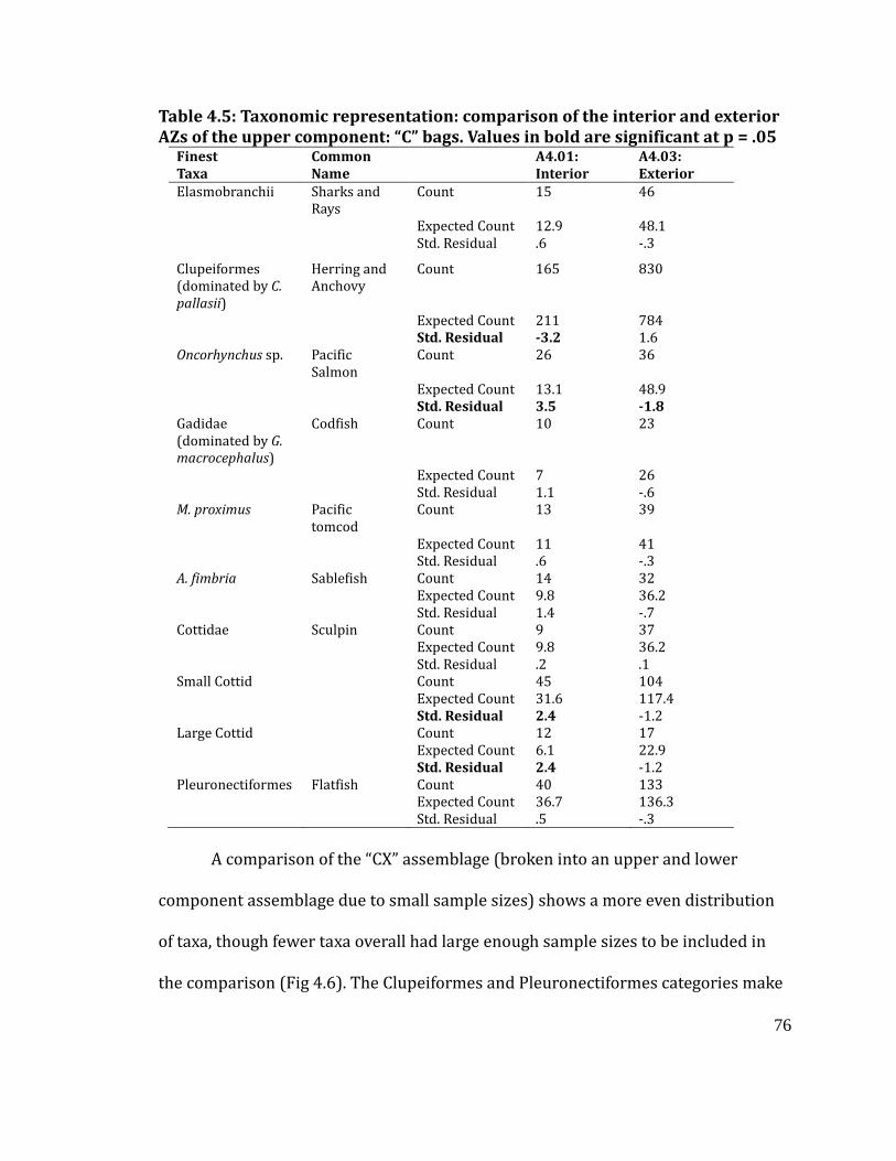
76

Table 4.5: Taxonomic representation: comparison of the interior and exterior

AZs of the upper component: “C” bags. Values in bold are significant at p = .05

A comparison of the “CX” assemblage (broken into an upper and lower

component assemblage due to small sample sizes) shows a more even distribution

of taxa, though fewer taxa overall had large enough sample sizes to be included in

the comparison (Fig 4.6). The Clupeiformes and Pleuronectiformes categories make

Finest

Taxa

Common

Name

A4.01:

Interior

A4.03:

Exterior

Elasmobranchii Sharks and

Rays

Count 15 46


Std. Residual .6 -.3

Clupeiformes

(dominated by C.

pallasii)

Herring and

Anchovy

Count 165 830

Expected Count 211 784


Oncorhynchus sp. Pacific

Salmon

Count 26 36



Gadidae

(dominated by G.

macrocephalus)

Codfish Count 10 23

Expected Count 7 26

Std. Residual 1.1 -.6

M. proximus Pacific

tomcod

Count 13 39

Expected Count 11 41


A. fimbria Sablefish Count 14 32


Std. Residual 1.4 -.7



Std. Residual .2 .1










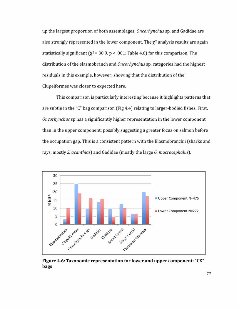
up the largest proportion of both

also strongly represented in the lower component.

statistically significant (

distribution of the elasmobranch

residuals in this example, however;

Clupeiformes was closer to expected

This comparison is particularly interesting because it highlights patterns that

are subtle in the “C” bag comparison (Fig 4.4)

Oncorhynchus sp has a significantly higher representation in the lower component

than in the upper component;

the occupation gap. This is a consistent pattern with the Elasmobranchii (sharks and

rays, mostly S. acanthias

Figure 4.6: Taxonomic representation for lowe

bags

0

5

10

15

20

25

30

% N

ISP

up the largest proportion of both assemblages; Oncorhynchus sp. and

also strongly represented in the lower component. The χ2 analysis results are again

significant (χ2 = 30.9, p < .001; Table 4.6) for this comparison

distribution of the elasmobranch and Oncorhynchus sp. categories had

in this example, however; showing that the distribution of the

Clupeiformes was closer to expected here.


he “C” bag comparison (Fig 4.4) relating to larger-bodied fishes

a significantly higher representation in the lower component

than in the upper component; possibly suggesting a greater focus on salmon before


S. acanthias) and Gadidae (mostly the large G. macrocephalus

Figure 4.6: Taxonomic representation for lower and upper componen

Upper Component N=475

Lower Component N=272

77

and Gadidae are

results are again

for this comparison. The

had the highest

showing that the distribution of the


bodied fishes. First,

a significantly higher representation in the lower component

focus on salmon before


G. macrocephalus).

r and upper component: “CX”

Upper Component N=475

Lower Component N=272

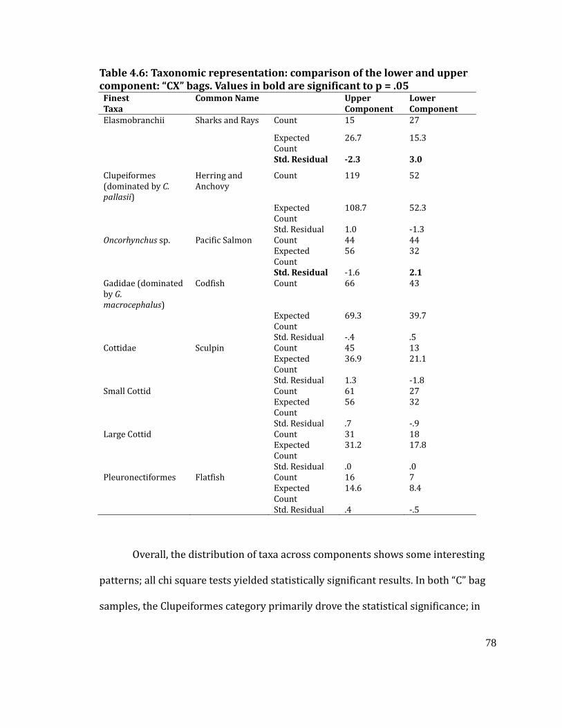
78

Table 4.6: Taxonomic representation: comparison of the lower and upper

component: “CX” bags. Values in bold are significant to p = .05

Overall, the distribution of taxa across components shows some interesting

patterns; all chi square tests yielded statistically significant results. In both “C” bag

samples, the Clupeiformes category primarily drove the statistical significance; in

Finest

Taxa

Common Name Upper

Component

Lower

Component

Elasmobranchii Sharks and Rays Count 15 27

Expected

Count

26.7 15.3


Clupeiformes

(dominated by C.

pallasii)

Herring and

Anchovy

Count 119 52

Expected

Count

108.7 52.3


Oncorhynchus sp. Pacific Salmon Count 44 44

Expected

Count

56 32


Gadidae (dominated

by G.

macrocephalus)

Codfish Count 66 43

Expected

Count

69.3 39.7



Expected

Count

36.9 21.1



Expected

Count

56 32



Expected

Count

31.2 17.8

Std. Residual .0 .0


Expected

Count

14.6 8.4


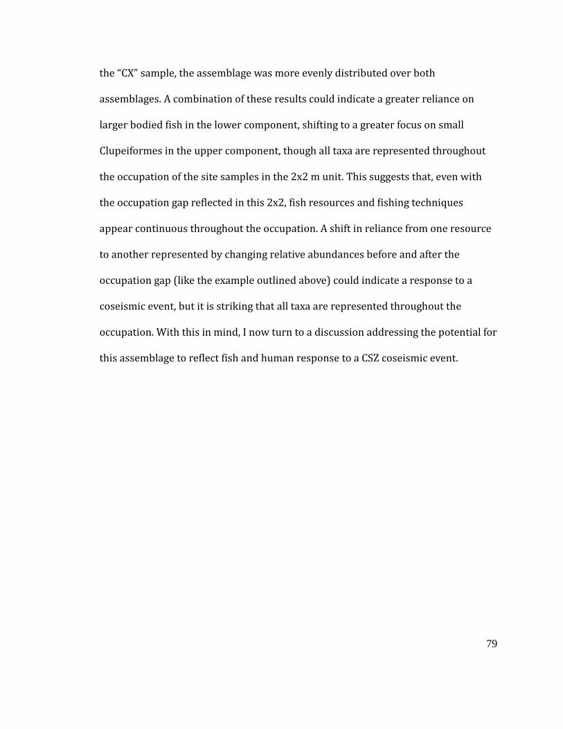
79

the “CX” sample, the assemblage was more evenly distributed over both

assemblages. A combination of these results could indicate a greater reliance on

larger bodied fish in the lower component, shifting to a greater focus on small

Clupeiformes in the upper component, though all taxa are represented throughout

the occupation of the site samples in the 2x2 m unit. This suggests that, even with

the occupation gap reflected in this 2x2, fish resources and fishing techniques

appear continuous throughout the occupation. A shift in reliance from one resource

to another represented by changing relative abundances before and after the

occupation gap (like the example outlined above) could indicate a response to a

coseismic event, but it is striking that all taxa are represented throughout the

occupation. With this in mind, I now turn to a discussion addressing the potential for

this assemblage to reflect fish and human response to a CSZ coseismic event.

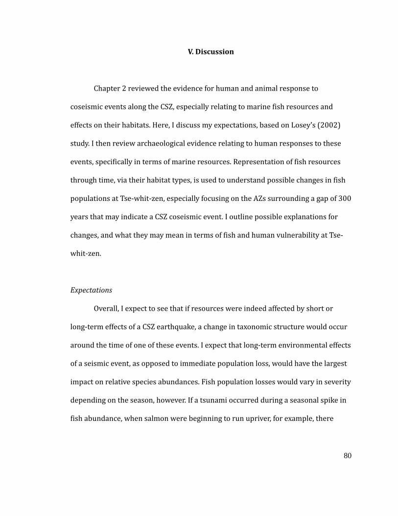
80

V. Discussion

Chapter 2 reviewed the evidence for human and animal response to

coseismic events along the CSZ, especially relating to marine fish resources and

effects on their habitats. Here, I discuss my expectations, based on Losey’s (2002)

study. I then review archaeological evidence relating to human responses to these

events, specifically in terms of marine resources. Representation of fish resources

through time, via their habitat types, is used to understand possible changes in fish

populations at Tse-whit-zen, especially focusing on the AZs surrounding a gap of 300

years that may indicate a CSZ coseismic event. I outline possible explanations for

changes, and what they may mean in terms of fish and human vulnerability at Tse-

whit-zen.

Expectations

Overall, I expect to see that if resources were indeed affected by short or

long-term effects of a CSZ earthquake, a change in taxonomic structure would occur

around the time of one of these events. I expect that long-term environmental effects

of a seismic event, as opposed to immediate population loss, would have the largest

impact on relative species abundances. Fish population losses would vary in severity

depending on the season, however. If a tsunami occurred during a seasonal spike in

fish abundance, when salmon were beginning to run upriver, for example, there

81

could have been a reduction of the population, which would have had a direct impact

on the people that relied on that seasonal abundance.

Habitat loss would be the most problematic for nearshore fish. Scouring of

the substrate from a tsunami would affect the nearshore bottom fish, including

species of flatfish. Loss of nearshore marine plants, habitat needed for many marine

species for shelter and spawning grounds, would have been problematic. Herring

populations, for example, spawning inshore at the time of a tsunami would have

suffered dramatic losses due to loss of eelgrass and kelp beds on which they deposit

their eggs.

It is also important to consider other alternatives for changes in relative fish

abundances post-earthquake, though the direct cause of the change in fish

abundance over time may be impossible to separate in the archaeological record.

Loss of important harvesting gear due to a tsunami could have made it much more

difficult for the human population to capture some of their important resources,

which could also explain changes in relative species abundance in the record. Loss of

boats would have made it impossible to capture larger bottom fish, such as red Irish

lord, cabezon, or sablefish. Loss of mass capture gear such as fish weirs, rakes, and

nets would have made it extremely difficult to harvest smaller, schooling fish such as

herring. The possible loss of technology may have been a factor in changes in

relative species abundances that show up within the archaeological record that have

nothing to do with effects on the fish populations themselves, but on the human

ability to capture them.

82

Overall, I expect that regardless of loss of fish habitat or loss of fishing gear

after a coseismic event, the observable response in the archaeological record would

be a shift to more nearshore fisheries. These shallow water fisheries may recover

faster than other habitats; Losey (2002) states eelgrass beds would be rejuvenated

quickly. Even if the sandy bottom was scoured away due to a tsunami, more silt

would be deposited as part of the tsunami as well, which further suggests this

particular habitat could rejuvenate faster than others. Furthermore, this shallow

water, sandy bottom habitat would not require as much specialized equipment to

access. If canoes, weirs, nets, and rakes were lost, these areas would still be

accessible to village occupants.

Habitat Assignment

In order to test my expectations relating to changes in relative species

abundance after a coseismic event at Tse-whit-zen, I grouped the fish taxa into

different habitat types. These habitat types, which are distinct foraging patches,

include the sandy substrate and eelgrass habitat, the rocky substrate and kelp forest

habitat, the Elwha River (salmon stream), and the open water (Fig 5.1). These four

habitat definitions allowed me to group fish taxa that could have been captured at

the same time, with similar technology, in order to simplify the attempt to track the

large number of different fish taxa through time.

The first habitat I defined as the nearshore, sandy substrate and eelgrass

habitat. This is a generalized patch nearest to the shore where a variety of small taxa

83

live year round. The next patch encompasses the slightly deeper water of the

nearshore environment, and is defined as the rocky substrate and kelp forest

habitat. Many rocky bottom fish live here year round, as well as fish that live in the

kelp forest and use it for food and shelter. These two habitats have year round

inhabitants, but also receive seasonal visitors that congregate during their breeding

cycles (e.g. Pacific herring). As such, these habitats are defined as generalized

patches, where fishers could have captured a variety of taxa at once.

The other two patches are targeted toward one species, and both have a

strong seasonal aspect. One of these targeted seasonal patches is the Elwha River,

which was an important salmon stream located about 10 km away from Tse-whit-

zen. Five salmonid species were historically reported to run up this stream yearly

(Pess et al. 2008), and fisherman could have traveled by canoe along the shore to

take advantage of these seasonal runs. The final patch is the open water, and

includes only Pacific herring. These fish were gathered with herring rakes in the

nearshore habitat when they congregated in the winter to spawn. Though they are

captured in the eelgrass/kelp forest habitats, I consider them separately in order to

understand any differences in CSZ earthquake effects on resident and highly mobile

fishes. Table 5.1 shows taxa assigned to each habitat type. Spiny dogfish, though

common in the assemblage, is not included in any grouping because it is

behaviorally different than any of these species, and did not fit well into any habitat

group. They are wanderers and can be caught near to shore. However, they do not

84

remain in the inshore environment and can be found in very deep water (Hart 1973,

Eschmeyer et al. 1983).

I then compared the changing reliance on each habitat type from the lower to

the upper component in order to track any changes in taxonomic abundances over

time. I did this with both the “C” and “CX” samples to see if the large bodied fish

sample contributed different information than the >1/8” “C” sample. If my

expectation was met, I would see a shift in the upper component away from fisheries

requiring specialized gear and away from fisheries in the deeper water habitats to

more shallow water fisheries.

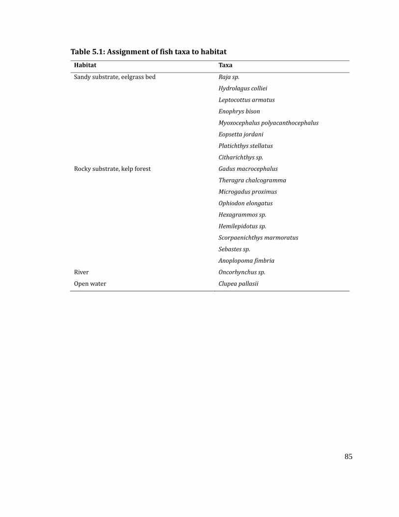
85

Table 5.1: Assignment of fish taxa to habitat

Habitat Taxa

Sandy substrate, eelgrass bed Raja sp.

Hydrolagus colliei

Leptocottus armatus

Enophrys bison

Myoxocephalus polyacanthocephalus

Eopsetta jordani

Platichthys stellatus

Citharichthys sp.

Rocky substrate, kelp forest Gadus macrocephalus

Theragra chalcogramma

Microgadus proximus

Ophiodon elongatus

Hexagrammos sp.

Hemilepidotus sp.

Scorpaenichthys marmoratus

Sebastes sp.

Anoplopoma fimbria

River Oncorhynchus sp.

Open water Clupea pallasii

Figure 5.1: Designation of habitat types surrounding Tse

Change Over Time in Habitat Use

Three AZs had large enough sample sizes to be compared: A4.05, A4.03, and

A4.01 (Fig 3.2). However, these

occupation break, and then both an inside and an outside portion of the upper

component, after the occupation break. This is sufficient for tracking changes

through time surrounding that gap

statistically significant difference in the distribution of these habitat types through

time (χ2 = 27.6, p < .001;

expected shifts.

: Designation of habitat types surrounding Tse-whit-zen

Change Over Time in Habitat Use

hree AZs had large enough sample sizes to be compared: A4.05, A4.03, and

. However, these three AZs encompass the time directly before the



through time surrounding that gap. A χ2 analysis of the “C” bag data shows


, p < .001; Table 5.2), though not all the habitat types followed the

86

zen

hree AZs had large enough sample sizes to be compared: A4.05, A4.03, and

three AZs encompass the time directly before the



analysis of the “C” bag data shows


), though not all the habitat types followed the

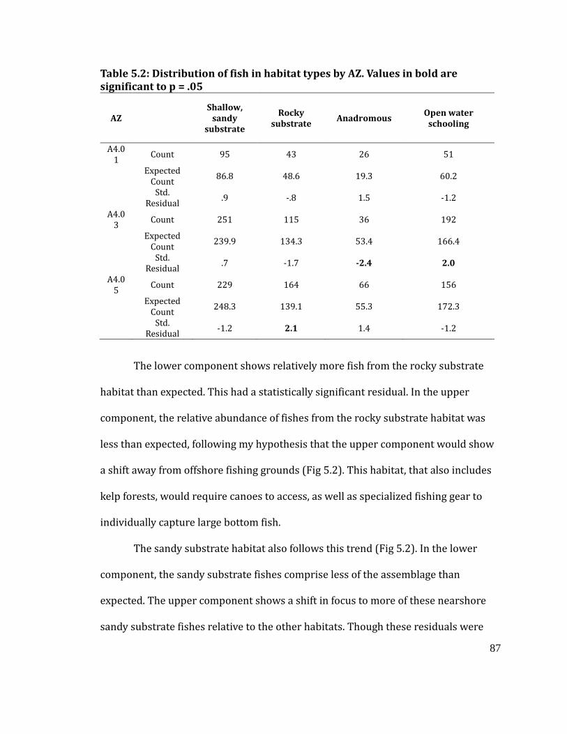
87

Table 5.2: Distribution of fish in habitat types by AZ. Values in bold are

significant to p = .05

AZ

Shallow,

sandy

substrate

Rocky

substrate Anadromous

Open water

schooling

A4.0

1 Count 95 43 26 51

Expected

Count 86.8 48.6 19.3 60.2

Std.

Residual .9 -.8 1.5 -1.2

A4.0

3 Count 251 115 36 192

Expected

Count 239.9 134.3 53.4 166.4

Std.

Residual .7 -1.7 -2.4 2.0

A4.0

5 Count 229 164 66 156

Expected

Count 248.3 139.1 55.3 172.3

Std.

Residual -1.2 2.1 1.4 -1.2

The lower component shows relatively more fish from the rocky substrate

habitat than expected. This had a statistically significant residual. In the upper

component, the relative abundance of fishes from the rocky substrate habitat was

less than expected, following my hypothesis that the upper component would show

a shift away from offshore fishing grounds (Fig 5.2). This habitat, that also includes

kelp forests, would require canoes to access, as well as specialized fishing gear to

individually capture large bottom fish.

The sandy substrate habitat also follows this trend (Fig 5.2). In the lower

component, the sandy substrate fishes comprise less of the assemblage than

expected. The upper component shows a shift in focus to more of these nearshore

sandy substrate fishes relative to the other habitats. Though these residuals were

88

not statistically significant, the trend follows my expectation. This habitat is home to

many smaller species, and does not require as elaborate fishing gear to procure as

offshore patches.

This pattern is more complicated when considering the two targeted species

habitats: the Elwha River (salmon) and open water (herring). Beginning with the

river, I would have expected a shift away from this resource in the upper component.

This is for two reasons. First, the salmon cycle itself could have suffered due to

altered river conditions post-tsunami. A tsunami could add silt to the water, change

the water temperature, alter the river bottom, and even create blockages in the river

preventing the salmon from getting to their spawning location. All of these factors

could prevent salmon from spawning, and could kill the alevins in the stream at the

time of the tsunami (Losey 2002, 2005). While the shift from A4.05 to A4.03 shows a

decreasing reliance on salmon that was statistically significant, the A4.01 sample,

also in the upper component, showed more salmon than expected.

The possible impacts affecting this resource are variable, however. Salmon

have a strong seasonal pattern, only gathering to run upstream and spawn at certain

time of the year. If a tsunami struck when these fish were far out to sea, this resource

would be much less affected, which could explain the relative consistency of this

resource before and after the occupation gap.

The herring (open water habitat) do not follow this pattern either.

Significantly more herring than expected were present in A4.03; A4.05 and A4.01

have similar proportions of herring. This resource, captured with canoes and

89

herring rakes, gathers in high numbers nearshore to spawn in the winter (December

to February), depositing their eggs on kelp and eelgrass (Hart 1973). Since herring

rely on kelp and eelgrass for spawning habitat, and specialized equipment is

necessary for the capture of these fish, I expected to see the decline of herring after

the occupation gap. My results indicate that the relative abundances of herring

actually increase after the gap, converse to my expectation.

Again, this could be due to the season that the coseismic event occurred.

Unless the herring were inshore spawning, these large populations of schooling fish

would have been away from the nearshore environment, and out of danger. As

discussed above, eelgrass is expected to rebound quickly, so the habitat required for

herring to spawn could have already been rehabilitated by the time these fish came

inshore to spawn. For both salmon and herring, Tse-whit-zen inhabitants could have

had an opportunity to rebuild their gear before the seasonal congregations of

salmon and herring, again depending on the season that the event struck the village.

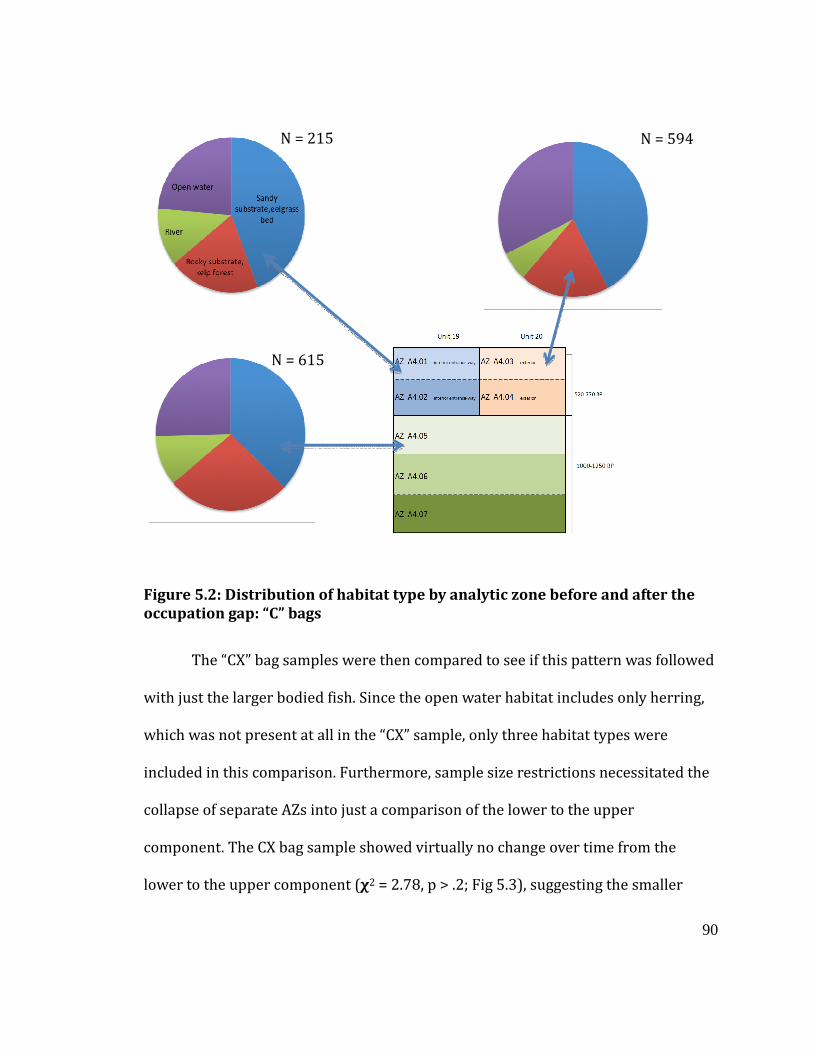
90

Figure 5.2: Distribution of habitat type by analytic zone before and after the

occupation gap: “C” bags

The “CX” bag samples were then compared to see if this pattern was followed

with just the larger bodied fish. Since the open water habitat includes only herring,

which was not present at all in the “CX” sample, only three habitat types were

included in this comparison. Furthermore, sample size restrictions necessitated the

collapse of separate AZs into just a comparison of the lower to the upper

component. The CX bag sample showed virtually no change over time from the

lower to the upper component (χ2 = 2.78, p > .2; Fig 5.3), suggesting the smaller

N = 215

N = 615

N = 594

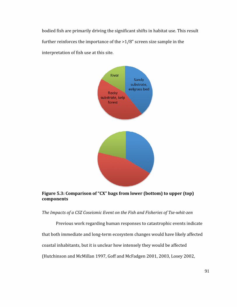
91

bodied fish are primarily driving the significant shifts in habitat use. This result

further reinforces the importance of the >1/8” screen size sample in the

interpretation of fish use at this site.

Figure 5.3: Comparison of “CX” bags from lower (bottom) to upper (top)

components

The Impacts of a CSZ Coseismic Event on the Fish and Fisheries of Tse-whit-zen

Previous work regarding human responses to catastrophic events indicate

that both immediate and long-term ecosystem changes would have likely affected

coastal inhabitants, but it is unclear how intensely they would be affected

(Hutchinson and McMillan 1997, Goff and McFadgen 2001, 2003, Losey 2002,

92

papers in Reycraft and Bawden 2000, Torrence and Grattan 2007). Some villages

were reoccupied after an event and abandoned after the next, some were

immediately abandoned, and some were never abandoned (Hutchinson and

McMillan 1997, Goff and McFadgen 2001, 2003). Some of the difficulty in

interpreting the precise nature of responses comes from the extreme variability in

how a coseismic event affects different parts of the coast. Coastal morphology,

seafloor bathymetry, elevation of the village above sea level, and many other factors

contribute to how severely an area and its resources would be affected (Saltonstall

and Carver 2002).

When studying these ideas at Tse-whit-zen, it appears that no clear response

to a coseismic event is visible. As shown above, the responses of the fish are more

complicated to predict; many specific conditions would have to be present for Tse-

whit-zen inhabitants to completely lose these resources due to a coseismic event. If

these conditions did converge, the result could have been disastrous for the

accumulation of winter stores and therefore survival of Tse-whit-zen inhabitants.

However, based on the consistency of these resources in the record from before and

after the occupation gap, it appears that the complete loss of these fisheries did not

occur at Tse-whit-zen.

Overall, these results indicate that, if a tsunami did strike the village and

cause the occupation gap, the fish populations may not have suffered great losses,

even in the years following the event. Additionally, even if the inhabitants were not

able to save any of their fishing gear, resources would have been available in the

93

nearshore habitat. Depending on the season of the coseismic event, inhabitants

could have even had time to rebuild their gear before the large seasonal gatherings

of salmon and herring occurred. This reinforces the argument presented previously

(Losey 2002, 2005, Saltonstall and Carver 2002): though these inhabitants relied on

the marine environment and lived in apparently vulnerable locations, coastal people

and their fish resources were ultimately resilient to the impacts of coseismic events.

The length of the occupation gap is problematic, however, in that we may be

completely missing the responses of fish and humans if a coseismic event did strike

Tse-whit-zen. Three hundred years could be ample time for the fish to rebound and

the residents of Tse-whit-zen to resume normal fishing practices, even considering a

very large earthquake. Though the patterns described above fit some of my

expectations, more 14C dates and further work in other areas of the site will be

necessary to resolve the timing of coseismic events and the nature of human and

animal responses to these events.

94

VI: Conclusions and Future Work

The extended time depth, large fish assemblage, and overlap with a CSZ

coseismic event in this 2x2m block presented an ideal starting point for attempting

to assess resource and human vulnerability to a coseismic event at Tse-whit-zen.

This assemblage is also comparable to other regional sites, providing a good record

of the full scale of fish use in these large coastal villages. After analyzing ~10,000

fish remains from two occupation components and assigning the identified taxa into

different habitat types, I assessed relative reliance on these different habitats

framing a ~300 year occupation gap that may indicate the impact of a CSZ coseismic

event. These results indicate that, though the generalized habitats follow my

expectations of a shift from offshore to nearshore reliance, fish taxa representing all

of the habitat types are present in each analytic zone, suggesting a striking amount

of continuity in fishing practices at this site and resilience to the effects of a

coseismic event.

Of additional value is that this work adds to the limited existing record of fish

use on the Strait of Juan de Fuca. Though much of this record agrees with local sites

(Hoko River and Ozette), some striking differences are present. Namely, the lack of

large numbers of rockfish, surfperch, greenling and the complete lack of plainfin

midshipman and lingcod in the Tse-whit-zen assemblage is striking in comparison to

these other sites. Additionally, relatively little salmon is present in this assemblage.

95

These discrepancies may be simply due to sampling, since this assemblage is only

from one 2x2 m unit. However, it is striking that such large discrepancies do exist;

further testing will show if this reflects truly different fishing practices between

these nearby sites.

In addition to these findings, this long-term record of fish use can inform on

modern ecological issues on the Olympic Peninsula, especially given the recent dam

removals on the Elwha River. The dams were installed in this river in the early 1900s

(Pess et al. 2008), and have prevented salmon from spawning upstream in this once-

important salmon stream since then. Since a major focus of the dam removal is the

rehabilitation of the Elwha River for salmon, the information from the excavation at

Tse-whit-zen can help inform on the pre-contact abundances of salmon in the Elwha

River. More work could resolve the species that were present, allowing fisheries

biologists and ecologists to become more informed of the salmon species that would

be using the Elwha to spawn.

In addition to the salmon focus surrounding the dam removal, the ~100

years of sediment build up behind the dams was released into the nearshore marine

habitats upon the removal of these dams (Shaffer et al. 2008, Warrick et al. 2008).

Recent concerns have been voiced about this excessive sediment load being

deposited overtop the nearshore kelp forest at the mouth of the Elwha River. The

taxonomic makeup of the fisheries at the village of Tse-whit-zen can contribute to

understanding the extent of kelp forests in this area: whether or not the kelp forest

is due to the dam installation or if it was native to this habitat. The relatively large

96

presence of rocky bottom and kelp-dwelling fish in the assemblage from Tse-whit-

zen suggests kelp forests may have been widespread even before the dams were

installed. Excavations closer to the river may resolve this, but clear archaeological

evidence of fish that inhabit the kelp forest could indicate this excessive modern

sedimentation is an issue that should be addressed to prevent their destruction.

This research is at the beginning of a multi-year project using faunal remains

to assess human response to abrupt and gradual environmental change at Tse-whit-

zen. This thesis has served to develop the beginning framework to this larger project

and also to establish the methodology for identification. I have used the fish remains

to examine the relative abundances of taxa through time to assess fisheries

vulnerability to coseismic events. This assemblage will then be added to the larger

fish assemblage from multiple structures, which will be compared to the mammal,

bird, and invertebrate record. The faunal record from different portions of the site

will be used to further clarify our understanding of changes in resource use through

time at Tse-whit-zen that could mirror human responses to abrupt and also gradual

environmental change.

97

Works Cited

Adams, John

1990 Paleoseismicity of the Cascadia Subduction Zone: Evidence from Turbidites

off the Oregon-Washington Margin. Tectonics 9: 569-583.

Ames, Kenneth M.

2002 Going by Boat: The Forager-Collector Continuum at Sea. In Beyond Foraging

and Collecting: Evolutionary Change in Hunter-Gatherer Settlement Systems,

edited by Ben Fitzhugh and Junko Habu, pp 19-52. Kluwer

Academic/Plenum Publishers. New York.

Ames, Kenneth M. and Herbert D. G. Maschner

1999 Peoples of the Northwest Coast: Their Archaeology and Prehistory. Thames

and Hudson, London.

Arima, Eugene

1983 The West Coast People: The Nootka of Vancouver Island and Cape Flattery.

British Columbia Provincial Museum Special Publication: 6. Victoria, British

Columbia.

Atwater, Brian F.

1987 Evidence for Great Holocene Earthquakes Along the Outer Coast of

Washington State. Science 236: 942-944.

Atwater, Brian F., Martitia P. Tuttle, Eugene S. Schweig, Charles M. Rubin, David K.

Yamaguchi, and Eileen Hemphill-Haley

2004 Earthquake Recurrence Inferred from Paleoseismology. In The Quaternary

Period in the United States, edited by A. R. Gillespie, S. C. Porter, and B. F.

Atwater, pp. 331-350. Developments in Quaternary Science, 1 (series editor,

Jim Rose). Elsevier, Amsterdam.

Atwater, Brian F., Musumi-Rokkaku Satoko, Satake Kenji, Tsuji Yoshinobu, Ueda

Kazue, and David K. Yamaguchi

2005 The Orphan Tsunami of 1700: Japanese Clues to a Parent Earthquake in North

America. U.S. Geological Survey, Reston, VA.

Bednarek, Angela

2001 Undamming Rivers: A Review of Ecological Impacts of Dam Removal.

Environmental Management 27: 803-814.

Benson, Boyd E., Brian F. Atwater, David K. Yamaguchi, Lorin J. Amidon, Sarah L.

Brown, and Roger C. Lewis.

98

2001 Renewal of Tidal Forests in Washington State after a Subduction Earthquake

in A.D. 1700. Quaternary Research 56: 139-147.

Butler, Virginia L.

1987 Fish Remains. In Duwamish No. 1 Site; A Lower Puget Sound Shell Midden.

University of Washington Office of Public Archaeology, Research Report 1.

1990 Distinguishing Natural from Cultural Salmonid Deposits in Pacific Northwest

North America. Unpublished Ph. D. Dissertation, University of Washington,

Seattle, Washington.

1993 Natural vs. Cultural Salmonid Remains: Origin of the Dalles Roadcut Bones,

Columbia River, Oregon. Journal of Archaeological Science 20: 1-24.

1996 Tui Chub Taphonomy and the Importance of Marsh Resources in the

Western Great Basin of North America. American Antiquity 61: 699-

717.

Butler, Virginia L. and James C. Chatters

1994 The Role of Bone Density in Structuring Prehistoric Salmon Bone

Assemblages. Journal of Archaeological Science 21: 413-424.

Byram, R. Scott

2002 Brush Fences and Basket Traps: The Archaeology and Ethnohistory of

Tidewater Weir Fishing on the Oregon Coast. Unpublished Ph.D.

dissertation, Department of Anthropology, University of Oregon, Eugene.

Campbell, Sarah K. and Virginia L. Butler

2011 Prehistoric Native American Use of Animals on the Northwest Coast and

Plateau. In The Subsistence Economies of Indigenous North American Socities:

A Handbook, edited by Bruce D. Smith, pp. 83-111. Smithsonian Institution

Scholarly Press, Washington, D.C.

Cannon, Michael D.

1999 A Mathematical Model of the Effects of Screen Size on Zooarchaeological

Relative Abundance Measures. Journal of Archaeological Science 26: 205-

214.

Casteel, R.W.

1972 Some Archaeological Uses of Fish Remains. American Antiquity 37: 404-419.

1976 Fish Remains in Archaeology and Paleo-environmental Studies. Academic

Press, New York.

99

Clothier, Charles R.

1950 A Key to Some Southern California Fishes Based on Vertebral Characteristics.

Fish Bulletin No. 89, California Department of Natural Resources, Division

of Fish and Game, Bureau of Marine Fisheries.

Croes, Dale R. and Eric Blinman (editors)

1980 Hoko River: A 2500 Year Old Fishing Camp on the Northwest Coast of North

America. Washington State University Laboratory of Anthropology Reports

of Investigations No. 58. Hoko River Archaeological Project Contribution No.

1. Pullman, Washington.

Drucker, Philip

1965 Cultures of the North Pacific Coast. Chandler Publishing Company, Scranton.

Eschmeyer, William N., Earl S. Herald and Howard Hammann

1983 A Field Guide to Pacific Coast Fishes. Houghton Mifflin Company, New

York.

FAO

2005 Regional Workshop on Rehabilitation of Fisheries and Aquaculture in Coastal

Communities of Tsunami Affected Countries in Asia, 28 February – 1 March

2005. FAO Regional Office for Asia and the Pacific, Bangkok, Thailand. RAP

publication 2005/06.

Friedman, Edward and Dale R. Croes

1980 Fauna. In Hoko River: A 2500 Year Old Fishing Camp on the Northwest Coast of

North America. Edited by Dale R. Croes and Eric Blinman, Washington State

University Laboratory of Anthropology Reports of Investigations No. 58.

Hoko River Archaeological Project Contribution No. 1. Pullman, Washington.

Goff, James R. and Bruce G. McFadgen

2001 Catastrophic Seismic-Related Events and Their Impact on Prehistoric Human

Occupation, New Zealand. Antiquity 75: 155-182.

2003 Large Earthquakes and the Abandonment of Prehistoric Coastal Settlements

in 15th Century New Zealand. Geoarchaeology 18: 609-623.

Goldfinger, Chris, C. Hans Nelson, and Joel E. Johnson

2003 Holocene Earthquake Records from the Cascadia Subduction Zone and

Northern San Andreas Fault Based on Precise Dating of Offshore Turbidites.

Annual Review of Earth and Planetary Sciences 31:555-577.

Gordon, Elisabeth A.

1993 Screen Size and Differential Faunal Recovery: A Hawaiian Example. Journal

100

of Field Archaeology 20: 453-460.

Gowan, Charles, Kurt Stephenson, and Leonard Shabman

2005 The Role of Ecosystem Valuation in Environmental Decision Making:

Hydropower Relicensing and Dam Removal on the Elwha River. Ecological

Economics 56: 508-523.

Grattan, John and Robin Torrence (editors)

2007 Living Under the Shadow: The Cultural Impacts of Volcanic Eruptions. Left

Coast Press. Walnut Creek, CA.

Grayson, Donald K.

1981 The effects of sample size on some derived measures in vertebrate faunal

analysis. Journal of Archaeological Science 8: 77.

1984 Quantitative Zooarchaeology. Academic Press, New York.

Gregory, Stan, Hiram Li, and Judy Li

2002 The Conceptual Basis for Ecological Responses to Dam Removal. Bioscience

52: 713-723.

Gunther, Erna

1927 Klallam ethnography. University of Washington Publications in Anthropology

1(5): 171-314.

Guidoboni, Emanuela and John E. Ebel

2009 Earthquakes and Tsunamis in the Past: A Guide to Techniques in Historical

Seismology. Cambridge University Press, New York.

Hanna, G. Dallas

1966 Biological Effects of the Alaska Earthquake, March 17, 1964: General Report.

National Academy of Sciences, Washington, D.C.

Hart, J.L.

1973 Pacific Fishes of Canada. Fisheries Research Board of Canada, Volume 180.

Ottawa, Ontario.

Hemphill-Haley, Eileen

1995 Diatom Evidence for Earthquake-Induced Subsidence and Tsunami 300 Yr

Ago in Southern Coastal Washington. Geological Society of America Bulletin

107: 367–378.

Huber, Harriet R., Jeffrey C. Jorgensen, Virginia L. Butler, Greg Baker and Rebecca

Stevens

101

2011 Can salmonids (Oncorhynchus spp.) be identified to species using vertebral

morphometrics? Journal of Archaeological Science 38: 136-146.

Huelsbeck, David R.

1994 Mammals and Fish in the Subsistence Economy of Ozette. In Ozette

Archaeological Project Research Reports, Volume II: Fauna. Edited by Stephen

R. Samuels. Reports of Investigations 66, Washington State University

Department of Anthropology. Pullman, WA. National Park Service, Pacific

Northwest Regional Office, Seattle, WA.

Huelsbeck, David and Dale R. Croes

1980 Fish Habitat Zones. In Hoko River: A 2500 Year Old Fishing Camp on the

Northwest Coast of North America. Edited by Dale R. Croes and Eric Blinman,

Washington State University Laboratory of Anthropology Reports of

Investigations 58. Hoko River Archaeological Project Contribution No. 1.

Pullman, Washington.

Hutchinson, Ian and Alan D. McMillan

1997 Archaeological Evidence for Village Abandonment Associated with Late

Holocene Earthquakes at the Northern Cascadia Subduction Zone.

Quaternary Research 48: 79-87.

Jacoby, Gordon C., Daniel E. Bunker, and Boyd E. Benson

1997 Tree-ring Evidence for an A.D. 1700 Cascadia Earthquake in Washington and

Northern Oregon. Geology 29: 999-1002.

Kozloff, Eugene L.

1973 Seashore Life of Puget Sound, the Strait of Georgia, and the San Juan

Archipelago. University of Washington Press, Seattle, Washington.

Larson, L. (editor)

2006 Data Recovery Excavation and Archaeological Monitoring at the Tse-Whit-zen

Site (45CA523). Larson Anthropological Archaeological Services Limited, Gig

Harbor, Washington. Final report submitted to Washington State Department

of Transportation, Tumwater, Washington.

Lewarch, Dennis E. and Lynn L. Larson

2004 Final WSDOT Port Angeles Graving Dock Facility Treatment and Monitoring

Plans for the Tse-whit-zen Site (45CA523) and Shotwell Recycling Property

Recovery, Port Angeles, Clallam County, Washington. Larson

Anthropological Archaeological Services, Limited, Gig Harbor, Washington.

LAAS Technical Report #2004-05. Submitted to the Washington State

Department of Transportation, Olympic Region, Tumwater, Washington.

102

Losey, Robert

2002 Communities and Catastrophe: Tillamook Response to the AD 1700 Earthquake

and Tsunami, Northern Oregon Coast. Ph. D. Dissertation, University of

Oregon, Eugene, OR. University Microfilms International, Ann Arbor, MI.

2005 Earthquakes and Tsunami as Elements of Environmental Disturbance on the

Northwest Coast of North America. Journal of Anthropological Archaeology

24: 101-116.

Lyman, R. Lee

1995 Determining when rare (zoo-) archaeological phenomena are truly absent.

Journal of Anthropological Method and Theory 2: 369-412.

2008 Quantitative Paleozoology. Cambridge University Press, Cambridge.

Lyman, R. Lee and Kenneth M. Ames

2007 On the use of species-area curves to detect the effects of sample size.

Journal of Archaeological Science 34: 1985-1990.

Matson, R. G., and Gary Coupland

1994 The Prehistory of the Northwest Coast. Left Coast Press, Walnut Creek, CA.

McKechnie, Iain

2005 Five Thousand Years of Fishing at a Shell Midden in the Broken Group

Islands, Barkley Sound, British Columbia. Unpublished M.A thesis,

Department of Archaeology, Simon Fraser University, Burnaby.

McMillan, Alan D.

1999 Since the Time of the Transformers: The Ancient Heritage of the Nuu-chah-

nulth, Ditidaht, and Makah. UBC Press, Vancouver.

Miller, Bruce S., Charles A. Simenstad, Jeffrey N. Cross, Kurt L. Fresh, and S. Nancy

Steinfort

1980 Nearshore Fish and Macroinvertebrate Assemblages Along the Strait of Juan de

Fuca Including Food Habits of the Common Nearshore Fish. Marine

Ecosystems Analysis, Puget Sound Region. Seattle, Washington.

Minor, Rick and Wendy C. Grant

1996 Earthquake-Induced Subsidence and Burial of Late Holocene Archaeological

Sites, Northern Oregon Coast. American Antiquity 61: 772-781.

Moss, Madonna L.

2011 Northwest Coast: Archaeology as Deep History. SAA Press, Washington, D.C.

103

National Academy of Sciences

1971 The Great Alaskan Earthquake of 1964: Biology. National Academy of

Sciences, Washington D.C.

Newman, Thomas M.

1959 Tillamook Prehistory and its Relation to the Northwest Coast Culture Area.

Unpublished Ph.D. dissertation, University of Oregon, Eugene.

Oregon Department of Geology and Mineral Industries

1995 Cascadia Subduction Zone boundary. Electronic document,

www.ccalmr.ogi.edu/tsunami, accessed June 10, 2013.

Partlow, Megan A.

2006 Sampling Fish Bones: A Consideration of the Importance of Screen Size and

Disposal Context in the North Pacific. Arctic Anthropology 43: 67-79.

Pess, George R., Michael L. McHenry, Timothy J. Beechie, and Jeremy Davies

2008 Biological Impacts of the Elwha River Dams and Potential Salmonid

Responses to Dam Removal. Northwest Science 82: 72-90.

Peterson, Curt D., Kenneth M. Cruikshank, Mark E. Darien

2012 Coseismic Subsidence and Paleotsunami Run-Up Records from Latest

Holocene Deposits in the Waatch Valley, Neah Bay, Northwest Washington,

U.S.A.: Links to Great Earthquakes in the Northern Cascadia Margin. Journal

of Coastal Research 29: 157-172.

Ramachandran, S, S. Anitha, V. Balamurugan, K. Dharanirajan, K. Ezhil Vendhan,

Marie Irine Preeti Divien, A. Senthil Vel, I. Sujjahad Hussain and A. Udayaraj

2005 Ecological impact of tsunami on Nicobar Islands (Camorta, Katchal,

Nancowry and Trinkat). Current Science: 89: 195-200.

Reetz, Elisabeth C. Dennis E. Lewarch, Stephanie E. Trudel, Nichole Gillis, Hayley E.

Kanipe, Sarah L. Sterling, Donald E. Tatum, and Sherry Kekkonen

2006 Field Techniques. In Data Recovery Excavation and Archaeological Monitoring

at the Tse-whit-zen Site (45CA523),Clallam County, Washington, edited by L.

Larson, pp. 7-1:7-109. Larson Anthropological Archaeological Services

Limited, Gig Harbor, Washington. Submitted to Washington State Department

of Transportation, Olympia Region.

Reitz, Eizabeth J., and Elizabeth S. Wing

2008 Zooarchaeology, 2nd edition. Cambridge Manuals in Archaeology, Cambridge

University Press, Cambridge.

Reycraft, Richard M. and Garth Bawden

104

2000 Introduction. In Environmental Disaster and the Archaeology of Human

Response, edited by G. Bawden and R.M. Reycraft,1-10. Anthropological

Papers No. 7, Maxwell Museum of Anthropology, Albuquerque.

Sakamoto, Kazuo

1984 Interrelationships of the Family Pleuronectidae (Pisces: Pleuronectiformes).

Memoirs of the Faculty of Fisheries, Hokkaido University 31 (1,2): 95-215.

Saltonstall, Patrick and Gary A. Carver

2002 Earthquakes, Subsidence, Prehistoric Site Attrition and the Archaeological

Record: A View From the Settlement Point Site, Kodiak Archipelago, Alaska.

In Natural Disasters and Cultural Change, edited by R. Torrence and J. Grattan,

pp. 172-192. One World Archaeology Series Volume 45. Routledge, New York.

Satake, Kenji, Kelin Wang, and Brian F. Atwater

2003 Fault Slip and Seismic Moment of the 1700 Cascadia Earthquake Inferred

from Japanese Tsunami Descriptions. Journal of Geophysical Research

108(B11): 25-35.

Satake, Kenji and Brian F. Atwater

2007 Long-Term Perspectives on Giant Earthquakes and Tsunamis at Subduction

Zones. Annual Review of Earth and Planetary Sciences 35: 349-374.

Schultz, Stewart T.

1990 The Northwest Coast: A Natural History. Timber Press, Portland, OR.

Shaffer, J. Anne, Patrick Crain, Brian Winter, Cathy Lear, and Timothy J. Randle

2008 Nearshore Restoration of the Elwha River through Removal of the Elwha and

Glines Canyon Dams: An Overview. Northwest Science 82: 48-58.

Stanley, Kirk W.

1968 Effects of the Alaska Earthquake of March 27, 1964 on Shore Processes and

Beach Morphology. Geological Survey Professional Paper 543-J. U.S.

Government Printing Office, Washington, D.C.

Sterling, Sarah L., Adam Freeburg, and Christopher Milton

2013 Potential Uses for GIS in the Analysis of Deposits at Tse-whit-zen. Paper

presented at the 66th Annual Northwest Anthropological Conference,

Portland.

Sterling, Sarah L., Kristine M. Bovy, Virginia L. Butler, Sarah K. Campbell, Michael A.

Etnier

2011 Beyond the Palimpsest: Using High-Resolution Techniques to Evaluate

Household Scale Economic Strategies and Earthquake Response on the

105

Northwest Coast. Poster Presented at the 76th Annual Meeting of the Society

of American Archaeology, Sacramento.

Sterling, Sarah L., Dennis E. Lewarch, Donald E. Tatum, Jenny L. Dellert, Elizabeth C.

Reetz, Stephanie, E. Trudel, and Nichole Gillis

2006 Stratigraphy and Geoarchaeology of the Tse-whit-zen Site (45CA523). In

Data Recovery Excavation and Archaeological Monitoring at the Tse-whit-zen

Site (45CA523),Clallam County, Washington, edited by L. Larson, pp. 7-1:7-

109. Larson Anthropological Archaeological Services Limited, Gig Harbor,

Washington. Submitted to Washington State Department of Transportation,

Olympia Region.

Stiros, Stathis C.

2001 The AD 365 Crete Earthquake and Possible Seismic Clustering During the

Fourth and Sixth Centuries AD in the Eastern Mediterranean: A Review of

Historical and Archaeological Data. Journal of Structural Geology 23: 545-562.

Suttles, Wayne

1974 The Economic Life of the Coast Salish of Haro and Rosario Straits. Garland

Publishing, Inc, New York.

Suttles, Wayne (editor)

1990 Northwest Coast. Handbook of North American Indians Volume 7.

Smithsonian Institution, Washington D.C.

Swan, J. G.

1869 The Indians of Cape Flattery at the Entrance to the Strait of Juan de Fuca,

Washington Territory. Smithsonian Contributions to Knowledge, Collins,

Philadelphia.

Thomson, Richard E.

1981 Oceanography of the British Columbia Coast. Canadian Special Publication

of Fisheries and Aquatic Sciences 56, Ottawa, Ontario.

Torrence, Robin, and John Grattan (editors)

2002 Natural Disasters and Cultural Change. One World Archaeology Series Volume

45. Routledge, London.

Tveskov, Mark A. and Jon M. Erlandson

2003 The Haynes Inlet Wiers: Estuarine Fishing and Archaeological Site Visibility

on the Southern Cascadia Coast. Journal of Archaeological Science 30: 1023-

1035.

Warrick, Jonathan A., Guy R. Chochrane, Yael Sagy, and Guy Gelfenbaum

106

2008 Nearshore Substrate and Morphology Offshore of the Elwha River,

Washington. Northwest Science 82: 153-163.

Wheeler, Alwyne C. and Andrew K. Jones

1989 Fishes. Cambridge University Press, Cambridge.

Williams, Harry

1999 Foraminiferal Distributions in Tidal Marshes Bordering the Strait of Juan de

Fuca: Implications for Paleoseismicity Studies. Journal of Foraminiferal

Research 29: 196-208.

Woodward, John A.

1986 Prehistoric Shipwrecks on the Oregon Coast? Archaeological Evidence. In

Contributions to the Archaeology of Oregon, 1983-1986, edited by Kenneth M.

Ames, pp 219-264. Association of Oregon Archaeologists Occasional Papers

3.

Wunderlich, Robert C., BD Winter and JH Meyer

1994 Resotoration of the Elwha River Ecosystem. Fisheries 19(8) 11-19.

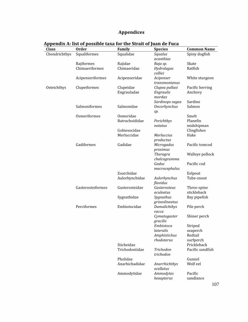
107

Appendices

Appendix A: list of possible taxa for the Strait of Juan de Fuca Class Order Family Species Common Name

Chondrichthys Squaliformes Squalidae Squalus

acanthias

Spiny dogfish

Rajiformes Rajidae Raja sp. Skate

Chimaeriformes Chimaeridae Hydrolagus

colliei

Ratfish

Acipenseriformes Acipenseridae Acipenser

transmontanus

White sturgeon

Osteichthys Clupeiformes Clupeidae Clupea pallasi Pacific herring

Engrauladae Engraulis

mordax

Anchovy

Sardinops sagax Sardine

Salmoniformes Salmonidae Oncorhynchus

sp.

Salmon

Osmeriformes Osmeridae Smelt

Batrachoididae Porichthys

notatus

Planefin

midshipman

Gobiesocidae Clingfishes

Merluccidae

Merluccius

productus

Hake

Gadiformes Gadidae Microgadus

proximus

Pacific tomcod

Theragra

chalcogramma

Walleye pollock

Gadus

macrocephalus

Pacific cod

Zoarchidae Eelpout

Aulorhynchidae Aulorhynchus

flavidus

Tube-snout

Gasterosteiformes Gasterosteidae Gasterosteus

aculeatus

Three-spine

stickleback

Sygnathidae Sygnathus

griseolineatus

Bay pipefish

Perciformes Embiotocidae Damalichthys

vacca

Pile perch

Cymatogaster

gracilis

Shiner perch

Embiotoca

lateralis

Striped

seaperch

Amphistichus

rhodoterus

Redtail

surfperch

Sticheidae Prickleback

Trichodontidae Trichodon

trichodon

Pacific sandfish

Pholidae Gunnel

Anarhichadidae Anarrhichthys

ocellatus

Wolf eel

Ammodytidae Ammodytes

hexapterus

Pacific

sandlance

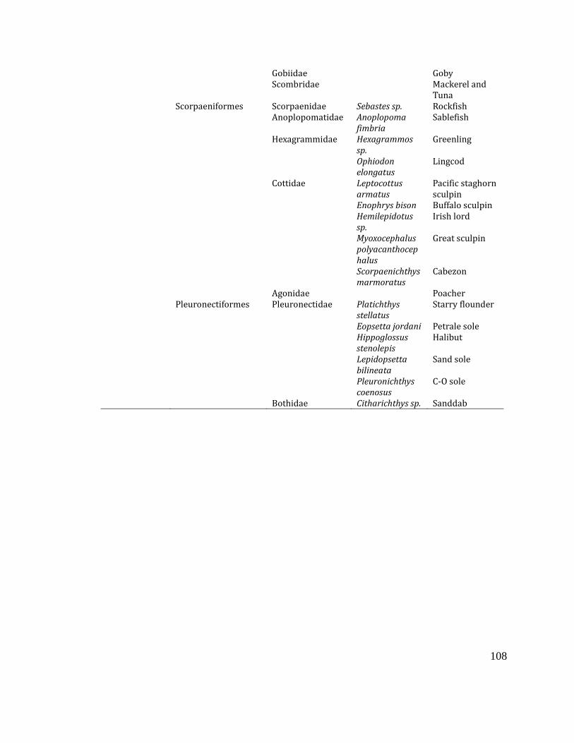
108

Gobiidae Goby

Scombridae Mackerel and

Tuna

Scorpaeniformes Scorpaenidae Sebastes sp. Rockfish

Anoplopomatidae Anoplopoma

fimbria

Sablefish

Hexagrammidae Hexagrammos

sp.

Greenling

Ophiodon

elongatus

Lingcod

Cottidae Leptocottus

armatus

Pacific staghorn

sculpin

Enophrys bison Buffalo sculpin

Hemilepidotus

sp.

Irish lord

Myoxocephalus

polyacanthocep

halus

Great sculpin

Scorpaenichthys

marmoratus

Cabezon

Agonidae Poacher

Pleuronectiformes Pleuronectidae Platichthys

stellatus

Starry flounder

Eopsetta jordani Petrale sole

Hippoglossus

stenolepis

Halibut

Lepidopsetta

bilineata

Sand sole

Pleuronichthys

coenosus

C-O sole

Bothidae Citharichthys sp. Sanddab

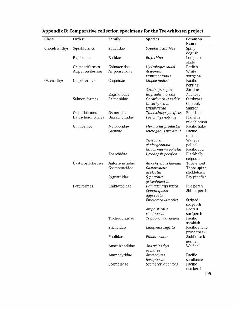
109

Appendix B: Comparative collection specimens for the Tse-whit-zen project

Class Order Family Species Common

Name

Chondrichthys Squaliformes Squalidae Squalus acanthias Spiny

dogfish

Rajiformes Rajidae Raja rhina Longnose

skate

Chimaeriformes Chimaeridae Hydrolagus colliei Ratfish

Acipenseriformes Acipenseridae Acipenser

transmontanus

White

sturgeon

Osteichthys Clupeiformes Clupeidae Clupea pallasi Pacific

herring

Sardinops sagax Sardine

Engrauladae Engraulis mordax Anchovy

Salmoniformes Salmonidae Oncorhynchus mykiss Cutthroat

Oncorhynchus

tshawytscha

Chinook

Salmon

Osmeriformes Osmeridae Thaleichthys pacificus Eulachon

Batrachoidiformes Batrachoididae Porichthys notatus Planefin

midshipman

Gadiformes Merluccidae Merluccius productus Pacific hake

Gadidae Microgadus proximus Pacific

tomcod

Theragra

chalcogramma

Walleye

pollock

Gadus macrocephalus Pacific cod

Zoarchidae Lycodopsis pacifica Blackbelly

eelpout

Gasterosteiformes Aulorhynchidae Aulorhynchus flavidus Tube-snout

Gasterosteidae Gasterosteus

aculeatus

Three-spine

stickleback

Sygnathidae Sygnathus

griseolineatus

Bay pipefish

Perciformes Embiotocidae Damalichthys vacca Pile perch

Cymatogaster

aggregata

Shiner perch

Embiotoca lateralis Striped

seaperch

Amphistichus

rhodoterus

Redtail

surfperch

Trichodontidae Trichodon trichodon Pacific

sandfish

Sticheidae Lumpenus sagitta Pacific snake

prickleback

Pholidae Pholis ornata Saddleback

gunnel

Anarhichadidae Anarrhichthys

ocellatus

Wolf eel

Ammodytidae Ammodytes

hexapterus

Pacific

sandlance

Scombridae Scombrer japonicas Pacific

mackerel

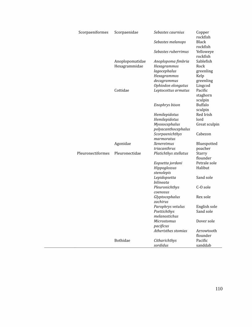
110

Scorpaeniformes Scorpaenidae Sebastes caurnius Copper

rockfish

Sebastes melanops Black

rockfish

Sebastes ruberrimus Yelloweye

rockfish

Anoplopomatidae Anoplopoma fimbria Sablefish

Hexagrammidae Hexagrammos

lagocephalus

Rock

greenling

Hexagrammos

decagrammus

Kelp

greenling

Ophiodon elongatus Lingcod

Cottidae Leptocottus armatus Pacific

staghorn

sculpin

Enophrys bison Buffalo

sculpin

Hemilepidotus

Hemilepidotus

Red Irish

lord

Myoxocephalus

polyacanthocephalus

Great sculpin

Scorpaenichthys

marmoratus

Cabezon

Agonidae Xeneretmus

triacanthrus

Bluespotted

poacher

Pleuronectiformes Pleuronectidae Platichthys stellatus Starry

flounder

Eopsetta jordani Petrale sole

Hippoglossus

stenolepis

Halibut

Lepidopsetta

bilineata

Sand sole

Pleuronichthys

coenosus

C-O sole

Glyptocephalus

zachirus

Rex sole

Parophrys vetulus English sole

Psettichthys

melanostichus

Sand sole

Microstomus

pacificus

Dover sole

Atheristhes stomias Arrowtooth

flounder

Bothidae Citharichthys

sordidus

Pacific

sanddab

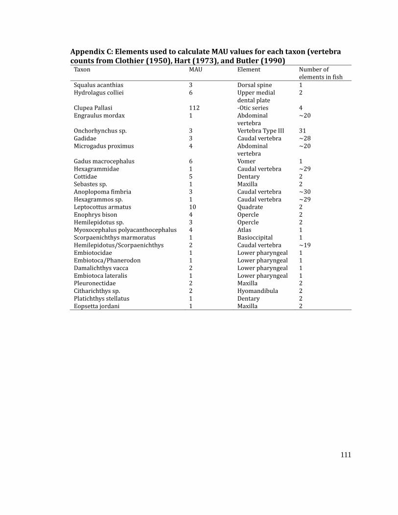
111

Appendix C: Elements used to calculate MAU values for each taxon (vertebra

counts from Clothier (1950), Hart (1973), and Butler (1990) Taxon MAU Element Number of

elements in fish

Squalus acanthias 3 Dorsal spine 1

Hydrolagus colliei 6 Upper medial

dental plate

2

Clupea Pallasi 112 -Otic series 4

Engraulus mordax 1 Abdominal

vertebra

~20

Onchorhynchus sp. 3 Vertebra Type III 31

Gadidae 3 Caudal vertebra ~28

Microgadus proximus 4 Abdominal

vertebra

~20

Gadus macrocephalus 6 Vomer 1

Hexagrammidae 1 Caudal vertebra ~29

Cottidae 5 Dentary 2

Sebastes sp. 1 Maxilla 2

Anoplopoma fimbria 3 Caudal vertebra ~30

Hexagrammos sp. 1 Caudal vertebra ~29

Leptocottus armatus 10 Quadrate 2

Enophrys bison 4 Opercle 2

Hemilepidotus sp. 3 Opercle 2

Myoxocephalus polyacanthocephalus 4 Atlas 1

Scorpaenichthys marmoratus 1 Basioccipital 1

Hemilepidotus/Scorpaenichthys 2 Caudal vertebra ~19

Embiotocidae 1 Lower pharyngeal 1

Embiotoca/Phanerodon 1 Lower pharyngeal 1

Damalichthys vacca 2 Lower pharyngeal 1

Embiotoca lateralis 1 Lower pharyngeal 1

Pleuronectidae 2 Maxilla 2

Citharichthys sp. 2 Hyomandibula 2

Platichthys stellatus 1 Dentary 2

Eopsetta jordani 1 Maxilla 2

Documents

Tracking Fish and Human Response to Abrupt Environmental